\jyear

2022

1]Guangxi Key Laboratory for Relativistic Astrophysics, School of Physical Science and Technology, Guangxi University, Nanning 530004, China 2]INAF Istituto di Astrofisica e Planetologia Spaziali, Via del Fosso del Cavaliere 100, 00133 Roma, Italy 3]INAF Osservatorio Astrofisico di Arcetri, Largo Enrico Fermi 5, 50125 Firenze, Italy 4]Dipartimento di Fisica e Astronomia, Università degli Studi di Firenze, Via Sansone 1, 50019 Sesto Fiorentino (FI), Italy 5]Istituto Nazionale di Fisica Nucleare, Sezione di Firenze, Via Sansone 1, 50019 Sesto Fiorentino (FI), Italy 6]Department of Physics and Kavli Institute for Particle Astrophysics and Cosmology, Stanford University, Stanford, California 94305, USA 7]INAF Osservatorio Astronomico di Cagliari, Via della Scienza 5, 09047 Selargius (CA), Italy 8]Yamagata University,1-4-12 Kojirakawa-machi, Yamagata-shi 990-8560, Japan 9]Istituto Nazionale di Fisica Nucleare, Sezione di Torino, Via Pietro Giuria 1, 10125 Torino, Italy 10]NASA Goddard Space Flight Center; Greenbelt, MD 20771, USA 11]University of Maryland, Baltimore County, Baltimore, MD 21250, USA 12]Center for Research and Exploration in Space Science and Technology, NASA/GSFC, Greenbelt, MD 20771, USA 13]Instituto de Astrofísica de Andalucía—CSIC, Glorieta de la Astronomía s/n, 18008, Granada, Spain 14]INAF Osservatorio Astronomico di Roma, Via Frascati 33, 00040 Monte Porzio Catone (RM), Italy 15]Space Science Data Center, Agenzia Spaziale Italiana, Via del Politecnico snc, 00133 Roma, Italy 16]Istituto Nazionale di Fisica Nucleare, Sezione di Pisa, Largo B. Pontecorvo 3, 56127 Pisa, Italy 17]Dipartimento di Fisica, Università di Pisa, Largo B. Pontecorvo 3, 56127 Pisa, Italy 18]NASA Marshall Space Flight Center, Huntsville, AL 35812, USA 19]Dipartimento di Matematica e Fisica, Università degli Studi Roma Tre, Via della Vasca Navale 84, 00146 Roma, Italy 20]Dipartimento di Fisica, Università degli Studi di Torino, Via Pietro Giuria 1, 10125 Torino, Italy 21]Agenzia Spaziale Italiana, Via del Politecnico snc, 00133 Roma, Italy 22]Istituto Nazionale di Fisica Nucleare, Sezione di Roma Tor Vergata, Via della Ricerca Scientifica 1, 00133 Roma, Italy 23]Institut für Astronomie und Astrophysik, Sand 1, 72076 Tübingen, Germany 24]Astronomical Institute of the Czech Academy of Sciences, Boční II 1401/1, 14100 Praha 4, Czech Republic 25]RIKEN Cluster for Pioneering Research, 2-1 Hirosawa, Wako, Saitama 351-0198, Japan 26]California Institute of Technology, Pasadena, CA 91125, USA 27]Osaka University, 1-1 Yamadaoka, Suita, Osaka 565-0871, Japan 28]University of British Columbia, Vancouver, BC V6T 1Z4, Canada 29]Department of Physics, Faculty of Science and Engineering, Chuo University, 1-13-27 Kasuga, Bunkyo-ku, Tokyo 112-8551, Japan 30]Institute for Astrophysical Research, Boston University, 725 Commonwealth Avenue, Boston, MA 02215, USA 31]Laboratory of Observational Astrophysics, St. Petersburg University, University Embankment 7/9, St. Petersburg 199034, Russia 32]Physics Department and McDonnell Center for the Space Sciences, Washington University in St. Louis, St. Louis, MO 63130, USA 33]Finnish Centre for Astronomy with ESO, Vesilinnantie 5, 20014 University of Turku, Finland 34]Université de Strasbourg, CNRS, Observatoire Astronomique de Strasbourg, UMR 7550, 67000 Strasbourg, France 35]MIT Kavli Institute for Astrophysics and Space Research, Massachusetts Institute of Technology, 77 Massachusetts Avenue, Cambridge, MA 02139, USA 36]Graduate School of Science, Division of Particle and Astrophysical Science, Nagoya University, Furo-cho, Chikusa-ku, Nagoya, Aichi 464-8602, Japan 37]Hiroshima Astrophysical Science Center, Hiroshima University, 1-3-1 Kagamiyama, Higashi-Hiroshima, Hiroshima 739-8526, Japan 38]Department of Physics, University of Hong Kong, Pokfulam, Hong Kong 39]Department of Astronomy and Astrophysics, Pennsylvania State University, University Park, PA 16801, USA 40]Université Grenoble Alpes, CNRS, IPAG, 38000 Grenoble, France 41]Department of Physics and Astronomy, University of Turku, 20014 Turku, Finland 42]Space Research Institute of the Russian Academy of Sciences, Profsoyuznaya Str. 84/32, Moscow 117997, Russia 43]Center for Astrophysics, Harvard & Smithsonian, 60 Garden St, Cambridge, MA 02138, USA 44]INAF Osservatorio Astronomico di Brera, via E. Bianchi 46, 23807 Merate (LC), Italy 45]Dipartimento di Fisica e Astronomia, Università degli Studi di Padova, Via Marzolo 8, 35131 Padova, Italy 46]Dipartimento di Fisica, Università degli Studi di Roma Tor Vergata, Via della Ricerca Scientifica, 00133 Roma, Italy 47]Mullard Space Science Laboratory, University College London, Holmbury St Mary, Dorking, Surrey RH5 6NT, UK 48]Anton Pannekoek Institute for Astronomy & GRAPPA, University of Amsterdam, Science Park 904, 1098 XH Amsterdam, The Netherlands

Vela pulsar wind nebula x-rays are polarized to near the synchrotron limit

Fei Xie^1,2 Corresponding author: xief@gxu.edu.cn Alessandro Di Marco² Fabio La Monaca² Kuan Liu¹ Fabio Muleri² Niccolò Bucciantini^3,4,5 Roger W. Romani⁶ Enrico Costa² John Rankin² Paolo Soffitta² Matteo Bachetti⁷ Niccolò Di Lalla⁶ Sergio Fabiani² Riccardo Ferrazzoli² Shuichi Gunji⁸ Luca Latronico⁹ Michela Negro^10,11,12 Nicola Omodei⁶ Maura Pilia⁷ Alessio Trois⁷ Eri Watanabe⁸ Iván Agudo¹³ Lucio A. Antonelli^14,15 Luca Baldini^16,17 Wayne H. Baumgartner¹⁸ Ronaldo Bellazzini¹⁶ Stefano Bianchi¹⁹ Stephen D. Bongiorno¹⁸ Raffaella Bonino^9,20 Alessandro Brez¹⁶ Fiamma Capitanio² Simone Castellano¹⁶ Elisabetta Cavazzuti²¹ Stefano Ciprini^15,22 Alessandra De Rosa² Ettore Del Monte² Laura Di Gesu²¹ Immacolata Donnarumma²¹ Victor Doroshenko²³ Michal Dovčiak²⁴ Steven R. Ehlert¹⁸ Teruaki Enoto²⁵ Yuri Evangelista² Javier A. Garcia²⁶ Kiyoshi Hayashida^27,† Jeremy Heyl²⁸ Wataru Iwakiri²⁹ Svetlana G. Jorstad^30,31 Vladimir Karas²⁴ Takao Kitaguchi²⁵ Jeffery J. Kolodziejczak¹⁸ Henric Krawczynski³² Ioannis Liodakis³³ Simone Maldera⁹ Alberto Manfreda¹⁶ Frédéric Marin³⁴ Andrea Marinucci²¹ Alan P. Marscher³⁰ Herman L. Marshall³⁵ Francesco Massaro^9,20 Giorgio Matt¹⁹ Ikuyuki Mitsuishi³⁶ Tsunefumi Mizuno³⁷ C.-Y. Ng³⁸ Stephen L. O’Dell¹⁸ Chiara Oppedisano⁹ Alessandro Papitto¹⁴ George G. Pavlov³⁹ Abel L. Peirson⁶ Matteo Perri^14,15 Melissa Pesce-Rollins¹⁶ Pierre-Olivier Petrucci⁴⁰ Andrea Possenti⁷ Juri Poutanen^41,42 Simonetta Puccetti²¹ Brian D. Ramsey¹⁸ Ajay Ratheesh² Carmelo Sgró¹⁶ Patrick Slane⁴³ Gloria Spandre¹⁶ Toru Tamagawa²⁵ Fabrizio Tavecchio⁴⁴ Roberto Taverna⁴⁵ Yuzuru Tawara³⁶ Allyn F. Tennant¹⁸ Nicolas E. Thomas¹⁸ Francesco Tombesi⁴⁶ Sergey S. Tsygankov^41,42 Roberto Turolla^45,47 Jacco Vink⁴⁸ Martin C. Weisskopf¹⁸ Kinwah Wu⁴⁷ Silvia Zane⁴⁷ *Corresponding author: xief@gxu.edu.cn [ [ [ [ [ [ [ [ [ [ [ [ [ [ [ [ [ [ [ [ [ [ [ [ [ [ [ [ [ [ [ [ [ [ [ [ [ [ [ [ [ [ [ [ [ [ [ [

Pulsar wind nebulae are formed when outflows of relativistic electrons and positrons hit the surrounding supernova remnant or interstellar medium at a shock front. The Vela pulsar wind nebula is powered by a young pulsar (B0833-45, age 11 kyr) 1968Natur.220..340L and located inside an extended structure called Vela X, itself inside the supernova remnant 1985ApJ…299..828H . Previous X-ray observations revealed two prominent arcs, bisected by a jet and counter jet 2001ApJ…554L.189P ; 2001ApJ…556..380H . Radio maps have shown high linear polarization of 60 per cent in the outer regions of the nebula 2003MNRAS.343..116D . Here we report X-ray observation of the inner part of the nebula, where polarization can exceed 60 per cent at the leading edge, which approaches the theoretical limit of what can be produced by synchrotron emission. We infer that, in contrast with the case of the supernova remnant, the electrons in the pulsar wind nebula are accelerated with little or no turbulence in a highly uniform magnetic field.

Imaging X-ray Polarimetry Explorer (IXPE) 2021AJ….162..208S ; 2022JATIS…8b6002W provides a new X-ray view of the highest energy electrons near their acceleration sites. IXPE is a NASA/ASI explorer featuring three co-aligned X-ray telescopes each with an imaging photoelectric polarimeter detector unit based on a gas pixel detector Costa2001 ; 2021APh…13302628B . IXPE observed the Vela pulsar wind nebula (PWN) in two periods: (i) 2022-04-05 to 2022-04-15 and (ii) 2022-04-21 to 2022-04-30, with a total exposure of 860 ks. The data were extracted from the publicly available files processed by the IXPE Science Operations Center and analysed with standard tools as described in the supplementary Methods section.

Linear polarization is detected at high significance ( $\sim$ 31 $\sigma$ ) for the spatial- and energy-integrated Vela PWN in the 2–8 keV band. The linear polarization degree (PD) is (44.6 $\pm$ 1.4)% with a polarization angle (PA, also known as electric vector position angle EVPA, defined from North through East) of $-(50.0\pm$ 0.9)^∘, with 68.3% confidence level uncertainties. Previously, only the Crab PWN has been studied via X-ray polarization; the classic 1976, 1978 OSO-8 results 1976ApJ…208L.125W ; 1978ApJ…220L.117W have recently been confirmed by the Polarlight cube-sat 2020NatAs…4..511F . However, these observations provided only an integrated polarization measurement and the image-averaged polarization degree was less than half of that found here for Vela.

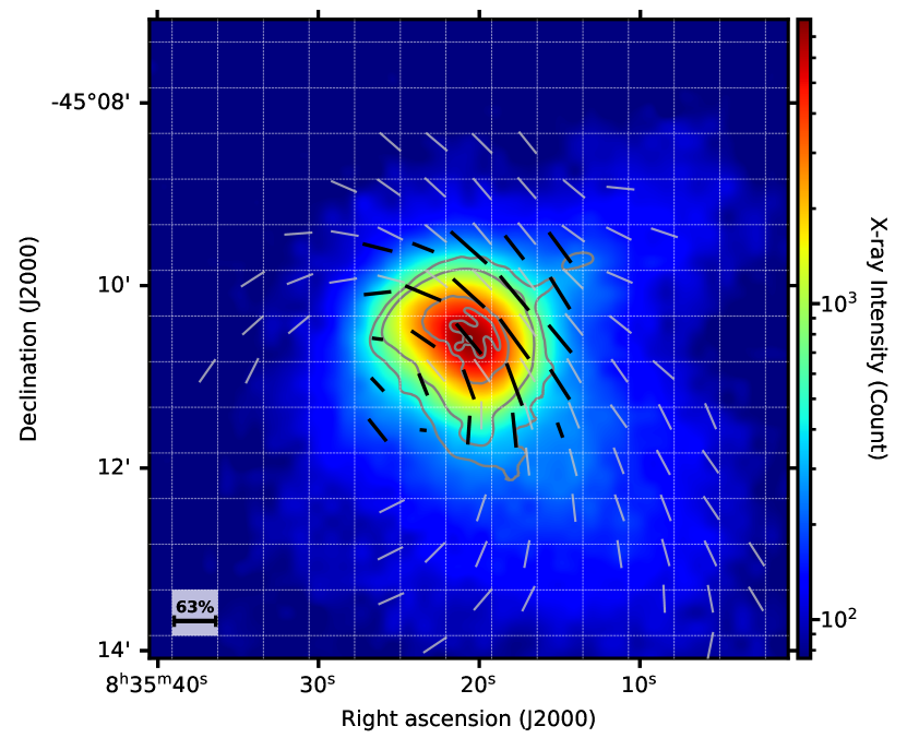
IXPE’s imaging capabilities, with a $\leq 30^{\prime\prime}$ half power diameter 2022JATIS…8b6002W , allow a spatially resolved polarimetric measurement of the PWN (Fig. 1). Here, 25 independent 30 ${}^{\prime\prime}\times$ 30^′′ square regions have been analyzed, combining data from the 3 detector units. The pulsar and compact arc-jet structure lie largely within the central region. The pulsar, dominated by a $kT\sim 0.13$ keV thermal component 2001ApJ…552L.129P , contributes less than 10% of the IXPE counts in this region. IXPE has not measured the polarization of the pulsed source; this may add to or subtract from the nebular polarization, but with the low flux (and low expected polarization degree Bucciantini et al ) the effect should be small. The black lines show linear polarization, with line length indicating polarization degree up to 62.8%. These lines are at 90^∘ to the EVPA, and thus show the direction of the projected magnetic field, which is highly symmetric about the pulsar jet axis.

The curved and symmetric polarization angle pattern seen in Fig. 1 implies that there will be some polarization angle variation across, and decrease in the region-average polarization degree of, our 25 measurement regions. This is most obvious to the sides and rear of the PWN, where the arcs seen in the Chandra image are highly curved and thus the underlying polarization angle varies rapidly, producing substantial de-polarization. Since the polarization follows the Chandra X-ray morphology we expect slightly higher polarization degree and smaller errors in regions where the arcs are less curved, which allows us to average over larger areas. As an example a morphologically selected region at the front of the nebula, along the symmetry axis provides a PD=70.0 $\pm$ 3.6% (Methods and Extended Data Fig. 5). As a caution, we note that for an analysis near the angular resolution limit in regions covering sharp intensity gradients, an effect due to the reconstruction of the photo-electron tracks in the gas pixel detector can artificially alter the local polarization values. Monte Carlo analysis show that this is a $\lesssim 5$ % effect, with a slight decrease in polarization degree to the North and increase to the South; our maximally polarized zones are hardly affected. Regardless, Vela’s high polarization degree and symmetric pattern imply a highly ordered magnetic field following the PWN’s toroidal structure.

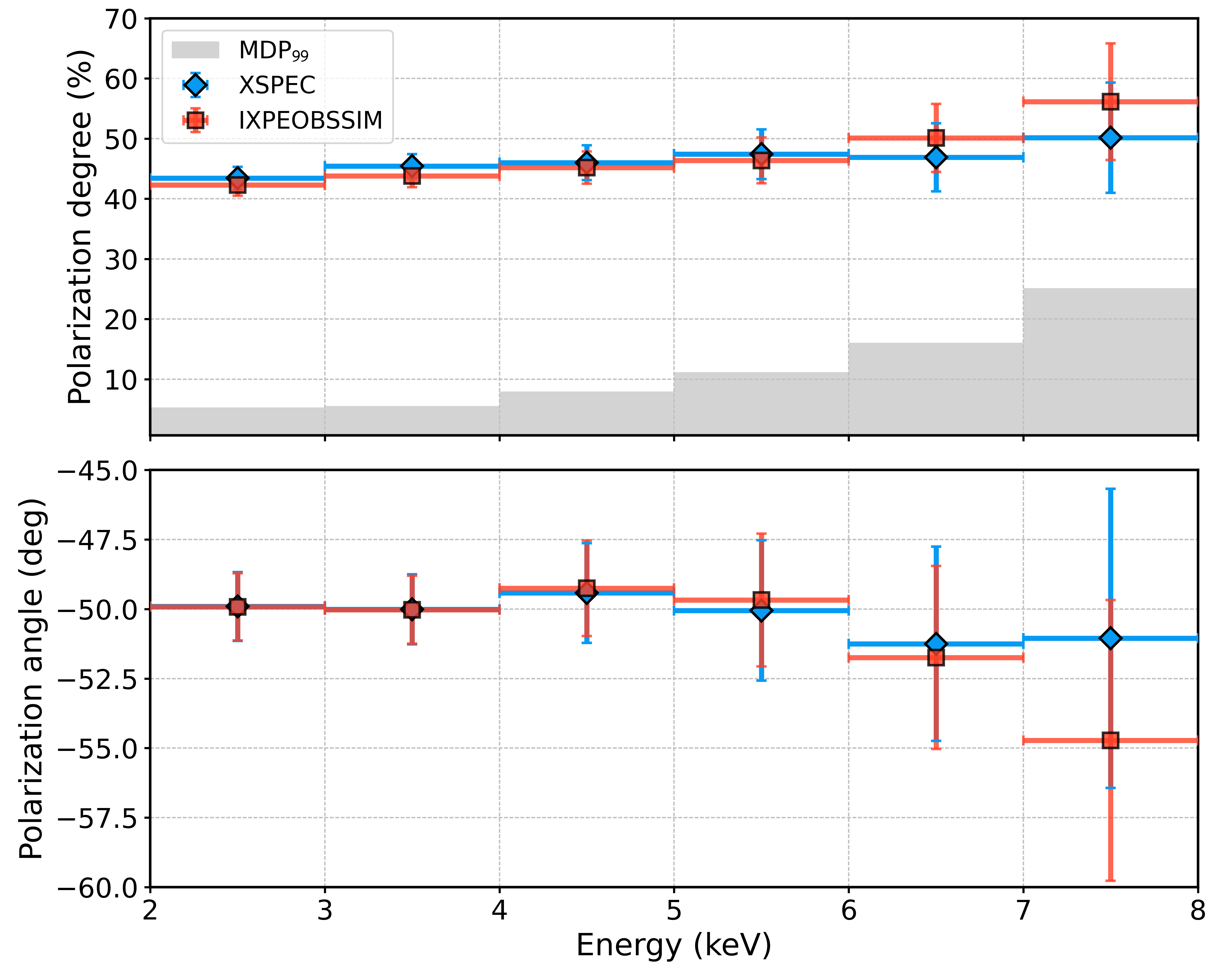
The spatially-averaged polarization of the Vela PWN is plotted as a function of energy in Fig. 2. A slight increase of polarization degree with energy is seen. This might be expected, since the emission region shrinks with increasing energy, thus arising from a smaller range of magnetic field orientations. The image-averaged polarization angle does not show significant energy dependence.

It is widely accepted that PWN arc-jet structures are due to an anisotropic pulsar wind, which generates toroidal magnetic fields in the equatorial zone 2004ApJ…601..479N ; 2002MNRAS.329L..34L ; 2003MNRAS.344L..93K ; 2004A&A…421.1063D . In this picture, the integrated polarization angle should align with the symmetry axis of the Vela PWN 2004MNRAS.349..779K ; 2005A&A…443..519B ; 2006A&A…453..621D , well consistent with the results reported here. The non-thermal radio and X-ray spectra of the Vela PWN already indicated domination by synchrotron emission. The high linear X-ray polarization, measured here for the first time with IXPE, strengthens this conclusion.

The maximum polarization degree of synchrotron radiation from a power law spectrum of electrons with index $p$ in a uniform magnetic field is $\Pi=(p+1)/(p+7/3)$ 1986rpa..book…..R ; the photon index $\Gamma$ of the emitted radiation is given by $p=2\Gamma-1$ . For Vela, with $\Gamma=1.3\pm 0.04$ in the compact jet-arc structure, increasing to 1.7 in the outskirts 2002ASPC..271..181K , the maximum polarization degree is 66–72%. Thus the 62.8% seen in Fig. 1 and Extended Data Table 3 (or the 70% in regions selected according to the Chandra image in Extended Data Table 4) is quite close to the maximum permitted value. This implies a magnetic field that is highly uniform across the measured region, with little turbulence-induced fluctuations. Also $\Gamma=1.3$ implies $p=1.6$ , appreciably flatter than the $p\approx 2.3-2.6$ of turbulent diffusive shock acceleration 2015SSRv..191..519S ; another mechanism, such as reconnection 2014ApJ…783L..21S , should play a dominant role in PWN particle energization.

The high uniformity and toroidal magnetic structure that we see with IXPE evidently extends to larger radii, where the $4^{\prime}$ radio lobes’ linear polarization indicates a magnetic field with a similar symmetry axis 2003MNRAS.343..116D (Fig. 1). Interestingly this magnetic structure is compressed to the North (evidently by the PWN interaction with the larger supernova remnant) and has a larger radius of curvature, centered behind the pulsar. With little radio emission from the X-ray bright torus/jet zone in the center, it appears that the radio tracks an older, cooler electron population centered behind the pulsar and extending to larger radii. Still, the substantial radio polarization, reaching 60% at both 5-GHz 2003MNRAS.343..116D and 1.4-GHz 2002ASPC..271..187B , indicates that the ordered and minimally turbulent fields probed by IXPE extend into this radio-emitting zone at much larger radii.

At present, we can say little about the X-ray polarization from the pulsar itself. Much deeper observations (and likely higher spatial resolution) will be required to isolate this component and compare with the optical phase average polarization of PD=8.1 $\pm 0.6$ % at PA=146.3 $\pm$ 2.4^∘2014MNRAS.445..835M . Like the Crab pulsar, Vela’s average optical polarization angle lies close to the projected torus axis. If, like the Crab pulsar, the phase-average X-ray polarization degree is well below that of the optical emission, corrections to our nebular estimates will be very small.

We find a remarkable high X-ray polarization in the Vela PWN, reaching an image- and energy-averaged polarization degree of $\sim$ 45%. The non-thermal PWN spectrum is bright in the IXPE energy band; the Vela pulsar itself emits mostly soft thermal X-rays, too faint and weakly polarized for detection at present. Our IXPE image sufficiently resolves the PWN to show that the polarization structure is symmetric about the projected pulsar spin (and proper motion) axis; this symmetry extends in radio polarization studies to even larger angles. The varying polarization angle across the nebula implies that the true local polarization is even larger and indeed we find polarization degree values $\geq$ 60% for some regions. This is close to the maximum polarization degree allowed for synchrotron emission with the observed X-ray spectrum, implying that the magnetic field is highly uniform across the emission region. Since electrons emitting synchrotron X-rays cool very rapidly, the IXPE X-rays are emitted close to the acceleration zone. In turn this argues against turbulence-driven diffusive shock acceleration and suggests that other processes, such as reconnection, should energize the PWN particles in the termination shock. Further IXPE studies of Vela and other bright PWNe should connect the X-ray polarization pattern with the details of the compact structures, further probing the physics of relativistic shock acceleration.

References

(1) \bibcommenthead
(2) Large, M. I., Vaughan, A. E. & Mills, B. Y. A Pulsar Supernova Association? Nature 220 (5165), 340–341 (1968).
(3) Harnden, J., F. R., Grant, P. D., Seward, F. D. & Kahn, S. M. Einstein observations of VELA X and the VELA pulsar. Astrophys. J. 299, 828–838 (1985).
(4) Pavlov, G. G., Kargaltsev, O. Y., Sanwal, D. & Garmire, G. P. Variability of the Vela Pulsar Wind Nebula Observed with Chandra. Astrophys. J. Lett. 554, L189–L192 (2001).
(5) Helfand, D. J., Gotthelf, E. V. & Halpern, J. P. Vela Pulsar and Its Synchrotron Nebula. Astrophys. J. 556, 380–391 (2001).
(6) Dodson, R., Lewis, D., McConnell, D. & Deshpande, A. A. The radio nebula surrounding the Vela pulsar. Mon. Not. R. Astron. Soc. 343, 116–124 (2003).
(7) Soffitta, P. et al. The Instrument of the Imaging X-Ray Polarimetry Explorer. Astron. J. 162, 208 (2021).
(8) Weisskopf, M. C. et al. The Imaging X-Ray Polarimetry Explorer (IXPE): Pre-Launch. J. Astron. Telesc. Instrum. Syst. 8 (2), 026002 (2022).
(9) Costa, E. et al. An efficient photoelectric x-ray polarimeter for the study of black holes and neutron stars. Nature 411, 662–665 (2001).
(10) Baldini, L. et al. Design, construction, and test of the Gas Pixel Detectors for the IXPE mission. Astropart. Phys. 133, 102628 (2021).
(11) Weisskopf, M. C. et al. Measurement of the X-ray polarization of the Crab nebula. Astrophys. J. Lett. 208, L125–L128 (1976).
(12) Weisskopf, M. C., Silver, E. H., Kestenbaum, H. L., Long, K. S. & Novick, R. A precision measurement of the X-ray polarization of the Crab Nebula without pulsar contamination. Astrophys. J. Lett. 220, L117–L121 (1978).
(13) Feng, H. et al. Re-detection and a possible time variation of soft X-ray polarization from the Crab. Nat. Astron. 4, 511–516 (2020).
(14) Pavlov, G. G., Zavlin, V. E., Sanwal, D., Burwitz, V. & Garmire, G. P. The X-Ray Spectrum of the Vela Pulsar Resolved with the Chandra X-Ray Observatory. Astrophys. J. Lett. 552, L129–L133 (2001).
(15) Bucciantini, N. et al. Simultaneous space and phase resolved X-ray polarimetry of the Crab Pulsar and Nebula. arXiv (2022).
(16) Lyubarsky, Y. E. On the structure of the inner Crab Nebula. Mon. Not. R. Astron. Soc. 329, L34–L36 (2002).
(17) Komissarov, S. S. & Lyubarsky, Y. E. The origin of peculiar jet-torus structure in the Crab nebula. Mon. Not. R. Astron. Soc. 344, L93–L96 (2003).
(18) Ng, C. Y. & Romani, R. W. Fitting Pulsar Wind Tori. Astrophys. J. 601, 479–484 (2004).
(19) Del Zanna, L., Amato, E. & Bucciantini, N. Axially symmetric relativistic MHD simulations of Pulsar Wind Nebulae in Supernova Remnants. On the origin of torus and jet-like features. Astron. Astrophys. 421, 1063–1073 (2004).
(20) Komissarov, S. S. & Lyubarsky, Y. E. Synchrotron nebulae created by anisotropic magnetized pulsar winds. Mon. Not. R. Astron. Soc. 349, 779–792 (2004).
(21) Bucciantini, N., del Zanna, L., Amato, E. & Volpi, D. Polarization in the inner region of pulsar wind nebulae. Astron. Astrophys. 443, 519–524 (2005).
(22) Del Zanna, L., Volpi, D., Amato, E. & Bucciantini, N. Simulated synchrotron emission from pulsar wind nebulae. Astron. Astrophys. 453, 621–633 (2006).
(23) Rybicki, G. B. & Lightman, A. P. Radiative Processes in Astrophysics (1986).
(24) Kargaltsev, O., Pavlov, G. G., Sanwal, D. & Garmire, G. P. The Vela Pulsar Wind Nebula Resolved with Chandra, Vol. 271 of Astronomical Society of the Pacific Conference Series, 181 (2002).
(25) Sironi, L., Keshet, U. & Lemoine, M. Relativistic Shocks: Particle Acceleration and Magnetization. Space Sci. Rev. 191, 519–544 (2015).
(26) Sironi, L. & Spitkovsky, A. Relativistic Reconnection: An Efficient Source of Non-thermal Particles. Astrophys. J. Lett. 783, L21 (2014).
(27) Bock, D. C. J., Sault, R. J., Milne, D. K. & Green, A. J. High-resolution Radio Polarimetry of Vela X. Neutron Stars in Supernova Remnants, Vol. 271 of Astronomical Society of the Pacific Conference Series, 187 (2002).
(28) Moran, P., Mignani, R. P. & Shearer, A. HST optical polarimetry of the Vela pulsar and nebula. Mon. Not. R. Astron. Soc. 445, 835–844 (2014).

Refer to caption — Figure 1: The IXPE intensity map of the Vela PWN in the 2–8 keV range with the measured X-ray polarization and radio polarization vectors overlaid. Intensity is the Gaussian-smoothed sum of the three detector units. The black lines present the X-ray polarization in the corresponding 30 ${}^{\prime\prime}\times$ 30^′′ image elements (white grids), their lengths indicate the polarization degree and the orientation indicates the projected magnetic field ( $90^{\circ}$ from the EVPA). The thinner silver lines, drawn with the same lengths, show the 5 GHz polarization directions derived from ref. 2003MNRAS.343..116D . The gray contours, obtained from Chandra observations in the same 2–8 keV range, give a better illustration of the pulsar, compact arc-jet structure, diffuse emission shell, and relatively weak outer jet (only weakly detected at IXPE resolution). The bar at the bottom left presents the maximum measured X-ray polarization degree of 63%, and the PD and PA in each of 25 grids are tabulated in Extended Data Table 3.

Methods

IXPE Data Analysis

This work is based on the polarimetric observations of the Vela pulsar and nebula obtained with the Imaging X-ray Polarimetry Explorer (IXPE), a NASA mission in partnership with the Italian space agency (ASI), as described in ref. 2021AJ….162..208S ; 2022JATIS…8b6002W and references therein. The IXPE Observatory includes three identical X-ray telescopes, each comprising an X-ray mirror assembly and a linear-polarization-sensitive detector, and performs imaging polarimetry over a nominal 2–8 keV energy band. IXPE data are telemetered to ground stations in Malindi (primary) and in Singapore (secondary), and are transmitted to the NASA Marshall Space Flight Center Science Operations Center (SOC) via the Mission Operations Center (MOC), at the Laboratory for Atmospheric and Space Physics, University of Colorado. Data are processed at the SOC, where raw data and relevant engineering/ancillary data are used to produce photon event lists. For each observation, the data are archived at the High-Energy Astrophysics Science Archive Research Center (HEASARC), at the NASA Goddard Space Flight Center for use by the international astrophysics community.

IXPE data are provided in two levels/formats: event_l1 and event_l2. The first level consists of unfiltered events; event_l2 files are produced from event_l1 after further calibration/correction procedures. In particular, event_l2 data are cleaned of in-flight-calibration data and occultation/SAA passages, then energy calibration/equalization of the three detector units (DUs) is applied and Stokes parameters are estimated following ref. 2015APh….68…45K . After this the spurious modulation is removed Rankin_2022 and the photons are referenced to sky coordinates, removing dithering pattern and boom motion effects.

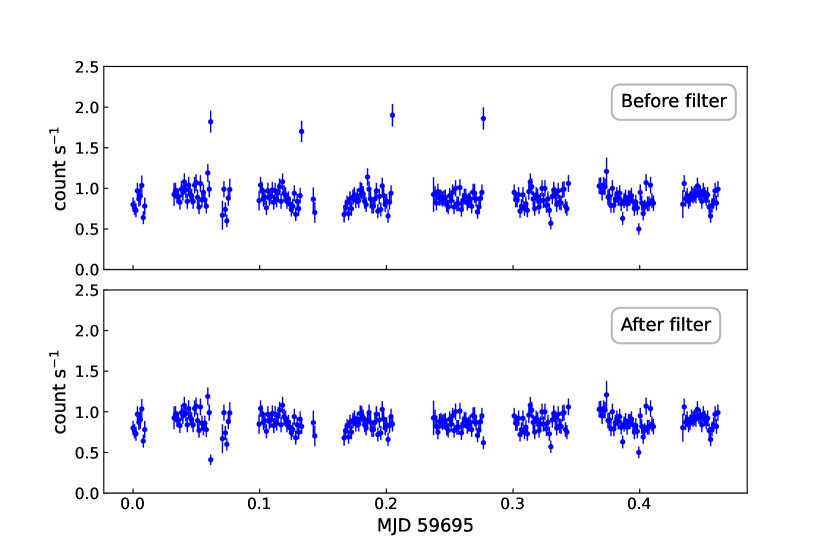
The Vela pulsar and PWN were observed with IXPE from 2022-04-05 at 19:51:40.687 UTC to 2022-04-15 at 18:08:18.343 UTC, and again from 2022-04-21 at 12:22:11.549 UTC to 2022-04-30 at 10:34:51.991 UTC, with net exposures 860 ks, 854 ks, 868 ks, respectively for the three DUs. After retrieving event_l2 files from the HEASARC, we performed three corrections: (1) energy correction (based on the onboard calibration data); (2) bad time interval filtering (to remove the solar flare events, see Extended Data Fig. 1); (3) barycenter correction (to convert the photon arrival time into the solar system barycenter; done with the standard HeaSoft 6.30.1 barycorr, with the following options: refframe=ICRS, ephem=JPLEPH.421). We find that the IXPE Vela observations were slightly affected by an increased particle flux during some portions of the orbit, associated with high solar activity.

Bad time intervals are identified as periods with count rates 3 $\sigma$ higher than average, assuming a Gaussian distribution. Events during such bad intervals are excluded from further data analysis.

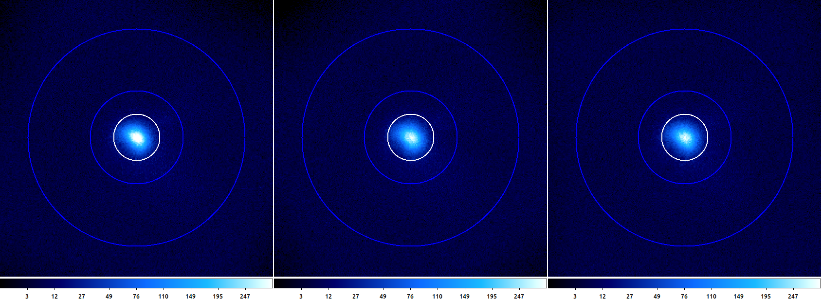
The field of view (FoV) of each detector is 12.9 ${}^{\prime}\times$ 12.9^′ (with the three detectors mounted at angles of 120^∘ to each other) 2022JATIS…8b6002W , while the X-ray emission of Vela PWN covers a much smaller region 2001ApJ…554L.189P . We identified source and background regions using the SAOImageDS9 software 2006ASPC..351..574J . The source region is a circle of radius 1^′ centered on the pulsar. The background region is an annulus with inner radius of 2^′ and outer radius of 4.7^′ (see Extended Data Fig. 2).

The polarization data consists of Stokes parameters ( $I$ , $Q$ , $U$ ) for each photon in the event_l2 files. For details on the Stokes parameters as defined in IXPE data see ref. Di_Marco_2022 . Data analysis was performed with different techniques and by different groups within the IXPE collaboration to cross-check the results. We first analyzed the data with the IXPE internal software ixpeobssim 2022arXiv220306384B , customized for IXPE data analysis and simulations. ixpeobssim includes tools developed to determine the source polarization properties via an analysis independent of the spectral models, following the unbinned method described in ref. 2015APh….68…45K . A second reduction is performed with xspec, using the version heasoft 6.30.1, which includes models for spectro-polarimetric analysis 2017ApJ…838…72S . With the binned spectra of the Stokes parameters, xspec performs standard forward-fitting and derives model-dependent polarization parameters. The adopted IXPE response functions are from the HEASARC IXPE CALDB March 14^th, 2022 release.

The spectral analysis shows that background events are not negligible at high energies, with rates becoming comparable (see Extended Data Fig. 3). To determine the source polarization while avoiding dilution effects at high energies, the background component was subtracted in all the analyses. The 2–8 keV band-averaged, aperture-averaged (1^′ radius) polarization degree and angle measurements are summarized in Extended Data Table LABEL:tab:spec_pol_energy_bin. The results are consistent between the three DUs and the two different analysis methods.

Spectro-polarimetric analysis is performed using xspec 1996ASPC..101…17A to jointly fit the three DUs in a two-step procedure. In the first step, the $I$ energy distribution are fitted with a spectral model. In the second step the spectral model is fixed, while $U$ and $Q$ are fit. This method thus does a forward folding fit to the binned spectra of the Stokes parameters $I$ , $Q$ , and $U$ jointly after fixing the spectral model.

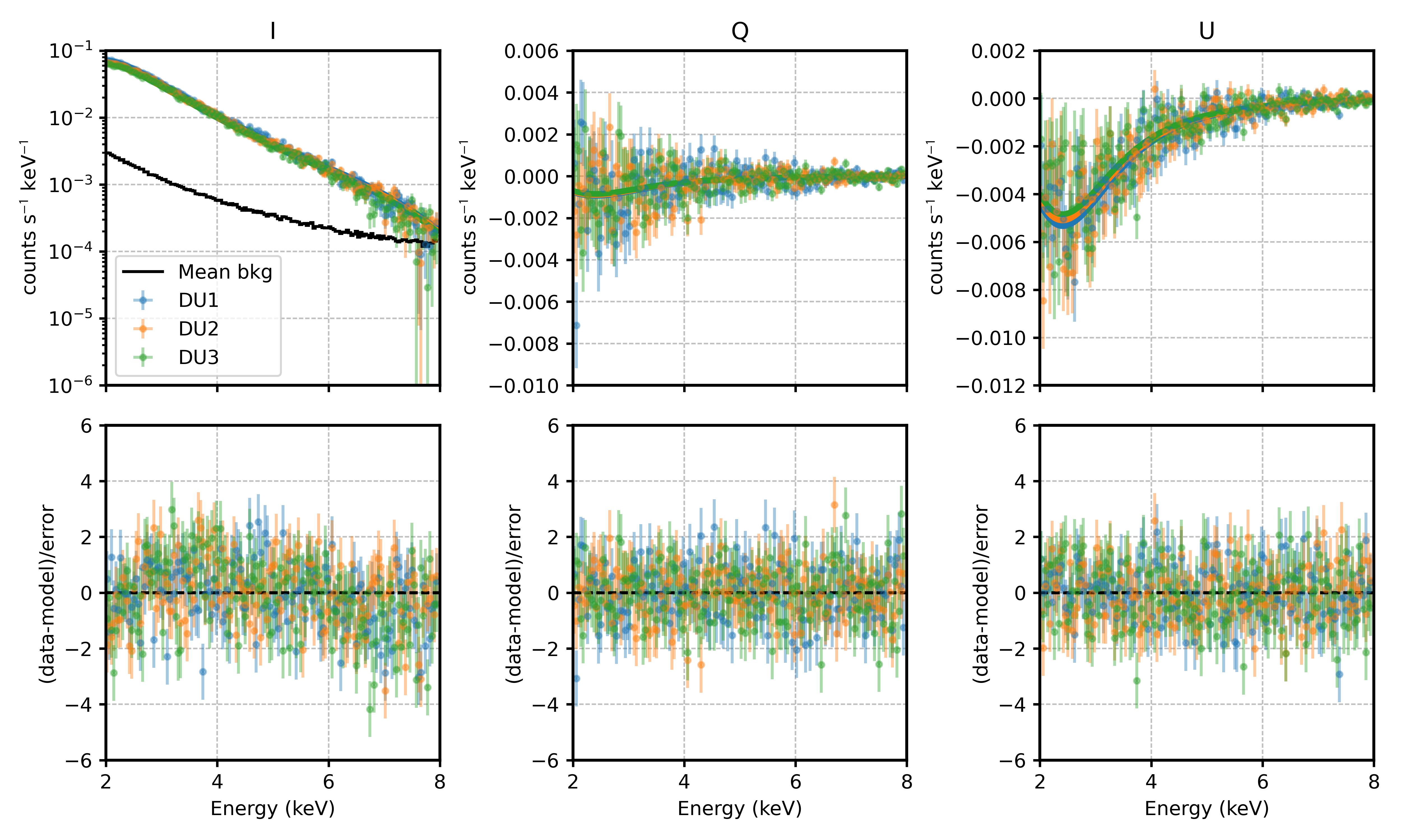
The Vela PWN binned $I$ spectra from the three DUs were fitted with the model factor*tbabs*powerlaw, where tbabs takes into account the interstellar absorption – here, we fixed the column density 2001ApJ…552L.129P to $N_{H}=0.03\times 10^{22}$ cm^-2 – a relative normalization factor for DU2 and DU3 accounts for uncertainties in their absolute effective area. The best-fit curves and the spectra of the Vela PWN for the three DUs are shown in Extended Data Fig. 3. At present, uncertainties in the effective area energy dependence are substantial, due to the incomplete knowledge of telescope alignment and related vignetting. Accordingly we focus on the polarization information. The spectral model parameters do not impact the polarization results, which are affected only by the energy assigned to individual photons. The individual photon energy estimate is tied to frequent in-flight calibration, performed with onboard calibration source during the Earth occultation. As the effective area variation becomes better understood, we expect the spectral model fitting to improve.

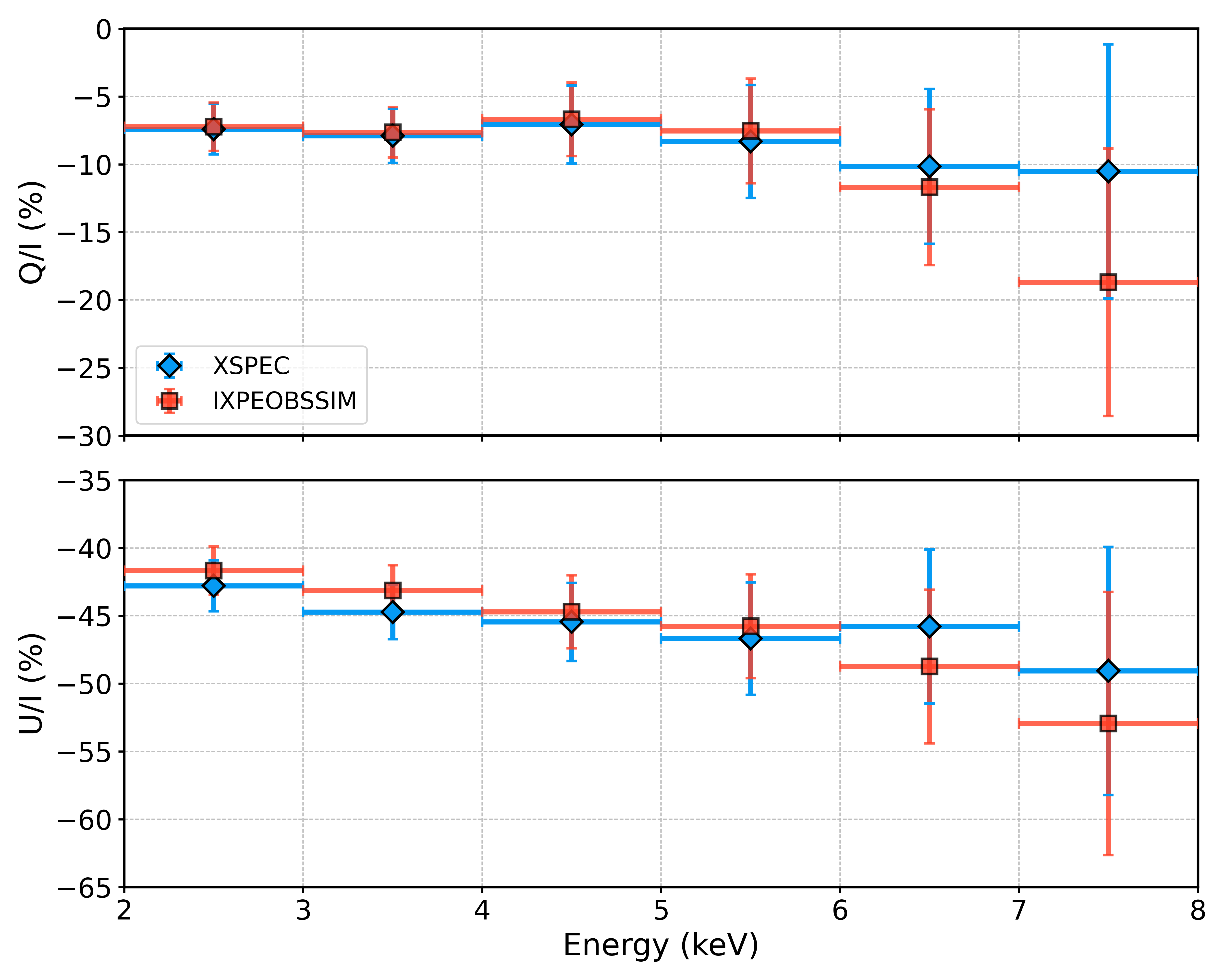
With the spectral model, binned $I$ , $Q$ , and $U$ spectra are fitted to obtain the polarimetric information, using the polarization model polconst of xspec. The fitted $I$ , $Q$ , $U$ spectra in the 2–8 keV energy band are shown in Extended Data Fig. 3. The polarization angle and degree obtained are in good agreement with those obtained by the model-independent analysis performed with ixpeobssim, as reported in Extended Data Table LABEL:tab:spec_pol_energy_bin.

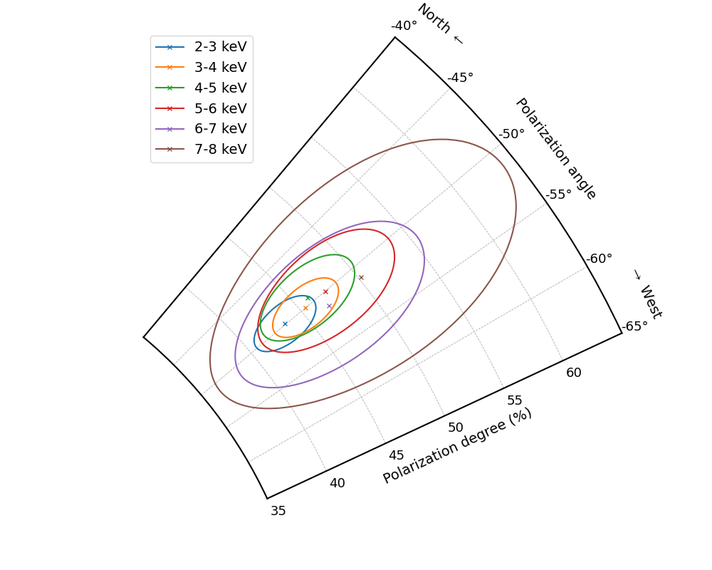
The same procedure was used to investigate the polarization in six energy bins fitting with xspec model factor*tbabs*powerlaw*polconst in each energy interval, freezing the $I$ spectral model parameters to the values previously obtained from the 2–8 keV analysis. Polarization degree and angle in each energy bin are reported in Extended Data Table LABEL:tab:spec_pol_energy_bin and Fig. 2. The ixpeobssim analysis is fully in agreement with that of xspec. PD and PA values obtained with xspec are represented in a 2D polar plot – with contours enclosing the 68.3% C.L. regions – in Extended Data Fig. 4. Similarly, $Q/I$ and $U/I$ Stokes parameters obtained with xspec and ixpeobssim are shown in Extended Data Fig. 6.

We have attempted to quantify the significance of the PD $(E)$ trend in Fig. 2. While a $\chi^{2}$ test finds that a constant PD is acceptable at the 57% level, a run-test analysis only accepts this hypothesis at 7.7% and a Kolmogorov-Smirnov test only has a probability of 3.6%. In contrast a linear PD $(E)$ model gives an acceptable $\chi^{2}$ probability at the 98% level, the run-test statistic is allowed at 41%, and a K-S test accepts the hypothesis at the 98% level. Thus a linear model with slope (1.8 $\pm$ 0.9) $\times 10^{-2}$ keV^-1, while not demanded by the data, is preferred over a simple constant PD model at the 2 $\sigma$ confidence level.

Spatially-resolved Analysis

Spatially-resolved analysis is performed with ixpeobssim. We divided the FoV into 30^′′ square bins, guided by the mirror PSF. Polarization analysis was performed for each bin, without background subtraction. Removing the background counts would give a small increase in the PD without affecting the PA. The statistics in the outer bins are poor, so we present only the results in 5 $\times$ 5 grids centered on the pulsar (Fig. 1). The tabulated results of the normalized $Q$ , $U$ , and their significance are in Extended Data Table 2, and the corresponding PD and PA are presented in Extended Data Table 3.

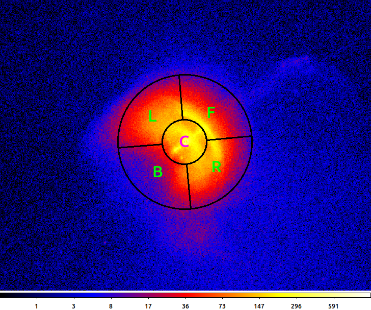
We also analyze the polarization parameters in five larger regions, aligned to the PWN symmetry axis, labeled as $L$ , $R$ , $F$ , $B$ and $C$ in Extended Data Fig. 5. Here we use ixpeobssim and subtract a scaled off-source background. The results, tabulated in Extended Data Table 4, show a polarization degree increasing along the symmetry axis from $\sim 30\%$ ( $B$ region) up to $\sim 70\%$ ( $F$ region). As with the finer square grid, $L$ and $R$ side regions show PA symmetrically spread about PA for the symmetry axis region $C$ .

The effect of the Pulsar on the PWN Polarization

The 89 ms Vela pulsar’s X-rays are largely thermal and make a negligible contribution to the 2–8 keV PWN flux as a whole. Thus, they cannot significantly affect our image-averaged PD and PA. However, from high resolution Chandra images, we see that the pulsar contributes $\sim 10\%$ of the 2–8 keV flux in the central square region of Fig. 1 and so it might affect its polarization. To bound such effects, we measured the spectrum of the Vela pulsar using the Chandra observation obsid 218, processed through the standard pipeline with the CIAO 4.13 package and CALDB version 4.9.5. If the pulsar contributes an unpolarized background, the corrected nebula-only PD rises to 55%. If in contrasts the pulsar emission is 100% polarized parallel (perpendicular) to the PA measured for the central square region, then the pulsar-subtracted polarization falls (rises) to 39% (66%). These values are from DU1 measurements only since with the smallest half-power width the pulsar will be most severe for this DU. In practice, the pulsar polarization is quite low in the optical band (PD=8.1 $\pm$ 0.6% at PA=(146.3 $\pm$ 0.6)^∘) 2014MNRAS.445..835M , and, by analogy with the Crab, will be even lower in the X-rays, so the true effect should be close to the unpolarized case, boosting the inferred PWN central PD. We apply this correction to the central bin in Fig. 1. Follow-up IXPE studies may more tightly bound the polarization of the pulsed emission.

Data Availability

IXPE data are available through the NASA’s HEASARC data archive at https://heasarc.gsfc.nasa.gov. Other derived data, supporting the findings of this study, are available from the corresponding author upon request.

Code Availability

The High Energy Astrophysics Science Archive Research Center (HEASARC) developed the HEASOFT (HEASARC Software). We used the HEASOFT version 6.30.1 package for the spectro-polarimetric IXPE data analysis, available at: https://heasarc.gsfc.nasa.gov/docs/software/heasoft/. The proper instrument response functions are provided by the IXPE Team as a part of the IXPE calibration database released on 2022 March 14 and available in the HEASARC Calibration Database at: https://heasarc.gsfc.nasa.gov/docs/heasarc/caldb/caldb_supported_missions.html.

The software developed by IXPE collaboration is available publicly through the web-page https://ixpeobssim.readthedocs.io/en/latest/?badge=latest.

Information supporting the findings of this study is available from the corresponding author upon request.

References

\bibcommenthead
(1) Kislat, F., Clark, B., Beilicke, M. & Krawczynski, H. Analyzing the data from X-ray polarimeters with Stokes parameters. Astropart. Phys. 68, 45–51 (2015).
(2) Rankin, J. et al. An Algorithm to Calibrate and Correct the Response to Unpolarized Radiation of the X-Ray Polarimeter Onboard IXPE. Astron. J. 163, 39 (2022).
(3) Joye, W. A. New Features of SAOImage DS9. In Astronomical Data Analysis Software and Systems XV, vol. 351 of Astronomical Society of the Pacific Conference Series, 574 (2006).
(4) Di Marco, A. et al. A Weighted Analysis to Improve the X-Ray Polarization Sensitivity of the Imaging X-ray Polarimetry Explorer. Astron. J. 163, 170 (2022).
(5) Baldini, L. et al. ixpeobssim: a Simulation and Analysis Framework for the Imaging X-ray Polarimetry Explorer. arXiv (2022).
(6) Strohmayer, T. E. X-Ray Spectro-polarimetry with Photoelectric Polarimeters. Astrophys. J. 838, 72 (2017).
(7) Arnaud, K. A. XSPEC: The First Ten Years. In Astronomical Data Analysis Software and Systems V, vol. 101 of Astronomical Society of the Pacific Conference Series, 17 (1996).

Acknowledgements

The Imaging X ray Polarimetry Explorer (IXPE) is a joint US and Italian mission. The US contribution is supported by the National Aeronautics and Space Administration (NASA) and led and managed by its Marshall Space Flight Center (MSFC), with industry partner Ball Aerospace (contract NNM15AA18C). The Italian contribution is supported by the Italian Space Agency (Agenzia Spaziale Italiana, ASI) through contract ASI-OHBI-2017-12-I.0, agreements ASI-INAF-2017-12-H0 and ASI-INFN-2017.13-H0, and its Space Science Data Center (SSDC) with agreements ASI-INAF-2022-14-HH.0 and ASI-INFN 2021-43-HH.0, and by the Istituto Nazionale di Astrofisica (INAF) and the Istituto Nazionale di Fisica Nucleare (INFN) in Italy. This research used data products provided by the IXPE Team (MSFC, SSDC, INAF, and INFN) and distributed with additional software tools by the High-Energy Astrophysics Science Archive Research Center (HEASARC), at NASA Goddard Space Flight Center (GSFC). The research at Guangxi University was supported in part by National Natural Science Foundation of China (Grant No. 12133003). The research at Boston University was supported in part by National Science Foundation grant AST-2108622. I.A. acknowledges financial support from the Spanish “Ministerio de Ciencia e Innovación” (MCINN) through the “Center of Excellence Severo Ochoa” award for the Instituto de Astrofísica de Andalucía-CSIC (SEV-2017-0709) and through grants AYA2016-80889-P and PID2019-107847RB-C44.

Author contributions

F.X. led the data analysis and the writing of the paper. A.D.M. and F.L.M performed the spectro-polarimetric analysis and contributed to the manuscript. F.M. and J.R. contributed to data analysis and energy calibration of the data-set. K.L. and N.B. contributed to the data analysis and results interpretation. R.W.R. and L.L. helped revise the manuscript. E.C., P.S., M.B., S.F., R.F., M.P. and A.T. contributed to the interpretation of the results and to text revisions. N.D.L., S.G., N.O., M.N. and E.W. performed independent analysis of the data. The remaining members of the IXPE collaboration contributed to the design of the mission, to the calibration of the instrument, to definition its science case and to the planning of the observations. All authors provided inputs and comments on the manuscript.

Competing interests

The authors declare no conflicts of interest.

Extended Data

Extended Data Table 1: Polarization degree and angle in six different energy bands and in the full IXPE 2–8 keV band.

	2–3 keV	3–4 keV	4–5 keV	5–6 keV	6–7 keV	7–8 keV	2–8 keV
PD (%)^I	42.3 $\pm$ 1.8	43.8 $\pm$ 1.9	45.2 $\pm$ 2.7	46.4 $\pm$ 3.8	50.1 $\pm$ 5.7	56.1 $\pm$ 9.7	44.6 $\pm$ 1.4
PD (%)^X	43.4 $\pm$ 1.9	45.4 $\pm$ 2.0	46.0 $\pm$ 2.9	47.4 $\pm$ 4.1	46.9 $\pm$ 5.7	50.2 $\pm$ 9.2	44.9 $\pm$ 1.1
PA (^∘)^I	$-$ 49.9 $\pm$ 1.2	$-$ 50.0 $\pm$ 1.2	$-$ 49.3 $\pm$ 1.7	$-$ 49.7 $\pm$ 2.4	$-$ 51.7 $\pm$ 3.3	$-$ 54.7 $\pm$ 5.0	$-$ 50.0 $\pm$ 0.9
PA (^∘)^X	$-$ 49.9 $\pm$ 1.2	$-$ 50.0 $\pm$ 1.3	$-$ 49.4 $\pm$ 1.8	$-$ 50.0 $\pm$ 2.5	$-$ 51.2 $\pm$ 3.5	$-$ 51.1 $\pm$ 5.4	$-$ 50.0 $\pm$ 0.7

Polarization degree and polarization angle measured using ixpeobssim and xspec in six energy bands and 2–8 keV using three DUs. Uncertainties on the polarization degree and angle are calculated for a 68.3% confidence level, assuming that they are independent. The values from the two different methods are compatible within the uncertainties.
I

Values are obtained with ixpeobssim.
X

Values are obtained with xspec.

Extended Data Table 2: The normalized Stokes parameters and the detection significance within the bins of Fig. 1.

	-2^b	-1^b	0^b	1^b	2^b
	$0.33\pm$ 0.17	$0.20\pm$ 0.13	$0.07\pm$ 0.11	$-0.09\pm$ 0.13	$-0.14\pm$ 0.15	Q/I^c
2^a	$-0.18\pm$ 0.18	$-0.18\pm$ 0.13	$-0.61\pm$ 0.11	$-0.36\pm$ 0.13	$-0.45\pm$ 0.14	U/I^d
	$1.3$	$1.2$	$5.0$	$2.0$	$2.6$	Sig^e
	$0.32\pm$ 0.10	$0.34\pm$ 0.05	$0.05\pm$ 0.04	$-0.10\pm$ 0.07	$-0.21\pm$ 0.13	Q/I^c
1^a	$0.07\pm$ 0.10	$-0.34\pm$ 0.05	$-0.53\pm$ 0.04	$-0.56\pm$ 0.07	$-0.42\pm$ 0.13	U/I^d
	$2.5$	$9.7$	$12.9$	$7.6$	$3.1$	Sig^e
	$0.10\pm$ 0.09	$0.13\pm$ 0.04	$-0.09\pm$ 0.02	$-0.19\pm$ 0.04	$-0.08\pm$ 0.11	Q/I^c
0^a	$-0.03\pm$ 0.09	$-0.32\pm$ 0.04	$-0.48\pm$ 0.02	$-0.60\pm$ 0.04	$-0.43\pm$ 0.11	U/I^d
	$-$	$8.8$	$19.7$	$15.6$	$3.3$	Sig^e
	$-0.01\pm$ 0.12	$-0.20\pm$ 0.07	$-0.30\pm$ 0.04	$-0.44\pm$ 0.05	$-0.18\pm$ 0.12	Q/I^c
-1^a	$-0.20\pm$ 0.12	$-0.19\pm$ 0.07	$-0.53\pm$ 0.04	$-0.37\pm$ 0.05	$-0.40\pm$ 0.12	U/I^d
	$0.8$	$3.2$	$9.6$	$10.5$	$3.0$	Sig^e
	$-0.07\pm$ 0.15	$0.04\pm$ 0.13	$-0.35\pm$ 0.09	$-0.42\pm$ 0.11	$-0.13\pm$ 0.13	Q/I^c
-2^a	$-0.33\pm$ 0.15	$-0.01\pm$ 0.13	$0.05\pm$ 0.09	$-0.09\pm$ 0.12	$-0.11\pm$ 0.13	U/I^d
	$1.4$	$-$	$3.1$	$3.2$	$0.1$	Sig^e

a

The row number where 0 presents the center bin containing the pulsar.
b

The column number where 0 presents the center bin containing the pulsar.
c

The $Q$ / $I$ Stokes parameters with 68.3% confidence level error.
d

The $U$ / $I$ Stokes parameters with 68.3% confidence level error.
e

The significance ( $\sigma$ ) for the non-polarized hypothesis test, based on the standard normal distribution. The corresponding P value means the probability that a polarized signal is generated by a non-polarized source. Specifically, a significance of 2 $\sigma$ means that the probability that the emission is polarized reaches 95%. Conventionally, the minimum detectable polarization at 99% confidence level (MDP₉₉) corresponds to a significance of 2.33 $\sigma$ .
$-$

No significant polarization detection.

Extended Data Table 3: The Polarization degree and angle within the bins of Fig 1.

	-2^b	-1^b	0^b	1^b	2^b
2^a	37 $\pm$ 18	27 $\pm$ 13	61 $\pm$ 12	37 $\pm$ 13	47 $\pm$ 15	PD^c
2^a	$-14\pm$ 14	$-21\pm$ 14	$-41.7\pm$ 5.3	$-52\pm$ 10	$-53.8\pm$ 8.9	PA^d
1^a	33 $\pm$ 10	48.5 $\pm$ 5.0	53.5 $\pm$ 4.1	56.8 $\pm$ 7.1	47 $\pm$ 13	PD^c
1^a	6.3 $\pm$ 9.0	$-22.4\pm$ 3.0	$-42.2\pm$ 2.2	$-50.2\pm$ 3.6	$-58.2\pm$ 7.7	PA^d
0^a	$10.3\pm$ 8.8	34.4 $\pm$ 3.9	49.0 $\pm$ 2.5	62.8 $\pm$ 4.0	44 $\pm$ 11	PD^c
0^a	$-$ 7.4 $\pm$ 24	$-34.3\pm$ 3.3	$-50.3\pm$ 1.5	$-53.9\pm$ 1.9	$-50.5\pm$ 7.4	PA^d
-1^a	21 $\pm$ 12	27.5 $\pm$ 7.2	38.5 $\pm$ 4.0	57.1 $\pm$ 5.4	44 $\pm$ 12	PD^c
-1^a	$-47\pm$ 17	$-68.3\pm$ 7.5	$-70.0\pm$ 3.0	$-69.8\pm$ 2.7	$-57.3\pm$ 7.9	PA^d
-2^a	34 $\pm$ 15	$4.5^{+13}_{-4.5}$	34.9 $\pm$ 9.5	43 $\pm$ 12	17 $\pm$ 14	PD^c
-2^a	$-51\pm$ 13	$-6.0\pm$ 85	$86.1\pm$ 7.8	$-84.2\pm$ 7.6	$-70\pm$ 23	PA^d

Polarization degree and polarization angle measured using ixpeobssim. Uncertainties on the polarization degree and angle are calculated for a 68.3% confidence level, assuming that they are independent.
a

The row number where 0 presents the center bin containing the pulsar.
b

The column number where 0 presents the center bin containing the pulsar.
c

The polarization degree (%) with 68.3% confidence level error.
d

The polarization angel (^∘) with 68.3% confidence level error.

Extended Data Table 4: The polarization degree and angle in the five regions shown in Extended Data Fig. 5.

	Center	Front	Right	Left	Back
	[ C ]	[ F ]	[ R ]	[ L ]	[ B ]
PD (%)^S	49.6 $\pm$ 2.5	70.0 $\pm$ 3.6	56.0 $\pm$ 3.1	42.0 $\pm$ 3.0	33.3 $\pm$ 3.6
PD (%)^S+B	48.8 $\pm$ 2.5	65.4 $\pm$ 3.6	53.1 $\pm$ 3.1	39.9 $\pm$ 3.0	31.1 $\pm$ 3.7
PA (^∘)^S	$-$ 50.2 $\pm$ 1.5	$-$ 48.8 $\pm$ 1.5	$-$ 64.9 $\pm$ 1.6	$-$ 30.1 $\pm$ 2.1	$-$ 59.4 $\pm$ 3.1
PA (^∘)^S+B	$-$ 50.3 $\pm$ 1.5	$-$ 48.8 $\pm$ 1.6	$-$ 64.9 $\pm$ 1.7	$-$ 30.2 $\pm$ 2.2	$-$ 59.4 $\pm$ 3.4

Polarization degree and polarization angle in C, F, R, L, and B regions measured using ixpeobssim with and without background subtraction. Background regions are the same as shown in Extended Data Fig. 2. Uncertainties on the polarization degree and angle are calculated for a 68.3% confidence level, assuming that they are independent.
^S

Values are obtained with background subtraction.
^S+B

Values are obtained without background subtraction.