Removeing Noise From Simulated Events at The Main Drift Chamber of BESIII Using Convolutional Neural Networks

Abstract

BESIII is the particle detector of the Beijing Electron-Positron Collider, which is a $\tau$-charm factory working at energies around 4 GeV. The first part of the detector, around the collision site, is called the Main Drift Chamber, MDC. The events recorded at MDC are mixed with the background noise of various origins. On average, about 10% of the hits of an event are noises. Still, the noise level differs event by event, and some of the events might even get more noise hits than signal hits, making the analysis less efficient. The standard algorithms of the offline software system of BESIII reconstruct signal tracks using the polluted data. This reduces the reconstruction efficiency of high noise tracks. In this article, we test the idea of using supervised deep learning techniques to remove this noise beforehand. We generate Monte Carlo events, then mix them with noise hits coming from real data. At first, we use deep learning techniques to classify the hits based on their individual features. Then, we simplify every event to a 40 by 43 picture and use image recognition tools to remove the noise. The average noise level for these events with only two signal tracks is about 30%. On average, the techniques presented in this article can purify Bhabha events to nearly 99% while preserving about 99% of the signal tracks.

1 Introduction

MDC is a 2.6m long cylindrical drift chamber with an outer diameter of 1.6m. It has 6796 sense wires which are distributed in 43 layers. There are two levels of trigger filtration in BESIII before the data gets stored. The efficiency of this system is as high as 100% for Bhabha scattering, and 97.7% for any $J/\Psi$ decay mode [1]. At the same time, the background rate reduces significantly, from $10^{4}$ KHz to about 1 KHz out of 3 KHz, which is the rate of event storage on the offline system [1]. This is an efficient process, but still, one third of this data is uninteresting background. Furthermore, the number of hits of an event is typically between 100 to 200, which about 5 to 15 percent of them are noises. The standard packages used on the offline system should remove the rest of the noise. Basically, these packages find the tracks of interest by considering all the hits, and the noise is eventually left aside like background tracks. Therefore it is hard to analyze events with high levels of noise. Our motivation is to reduce noise beforehand with deep learning methods while keeping efficiency high.

We present the first phase of our project here, in which we worked with simulated Bhabha events. Working with these simple events is a suitable choice for starting this project. Moreover, BESIII events are, in general, very clean. Though the luminosity is high, still most of the events have only two or four signal tracks. Another notable point is that Bhabha events are useful for purposes such as accurate luminosity measurements. Initially, we look at the situation as a hit classification problem and form neural networks that can distinguish noise hits solely based on their features. The features, in general, include time and charge, but we here only work with raw-time values. For the next step, we form convolutional networks to look at the whole event at once and remove the noise. These models basically remove the noise by finding the tracks, just like the standard algorithms. We later continued this work with graph neural networks and with more complicated events. The results will show up in an upcoming paper soon. The lesson from those studies is that the networks we find here need little change for more complicated situations and are indeed applicable to them as well.

2 Data Generation

MDC maps the 3D image of the events to 2D by recording the hits, which show up as electric pulses at the end caps. Still, the whole 3D image of an event is reconstructable, thanks to the time of flight information and the fact that the sense wires are not all aligned. The wires in the straight layers are aligned with the $z$ axes. However, wires of the stereo layers have angles with this direction.

As mentioned above, we work with Bhabha events for the start. These scattering events only include two tracks of high energy electrons and positrons. The solenoid magnetic field at MDC is about 1 T. The diameter of the detector is about 1.6 m. Naturally, the tracks are straight lines. Having 43 layers means there are around 86 signal hits for each event. Bhwide generator is used to simulate these events [2]. We do not work with all the available information, which would be accessible for real data only after the reconstruction process. Instead, only what would be in the outcome of MDC is considered, which includes two geometrical dimensions plus the time that the hit happens and its electric charge value.

Next, we add noise to these events using another package of the offline system of the spectrometer called BESEventMixer [2]. This algorithm uses real data and randomly adds noise of various origins to the simulated events. The noise hits have only space and time related features. The added noise is therefore independent of the events as expected and is, on average, about 40 hits per event. Hence, about one third of our data is noise, and the neural networks that we form have the task of removing it. We simulated 80000 events, which was enough for our purposes here.

3 Fully Connected Networks

For the first step, we choose the regression approach to classify the hits into signal or background. The feature space has two space dimensions and one time dimension [Fig. 2]. We developed a neural network that is, in principle, able to learn a threshold in time for every cell of every layer that discriminates between signal and background. This is related to the time that the generated particle most likely reaches that point. Such a network cannot make use of the geometry of the trajectories, which is the motivation behind using convolutional networks introduced in the next section. In fact, all the hits are introduced to the network simultaneously and not as in individual events. Nonetheless, the outcome is better than a simple cut line in time for a few percents.

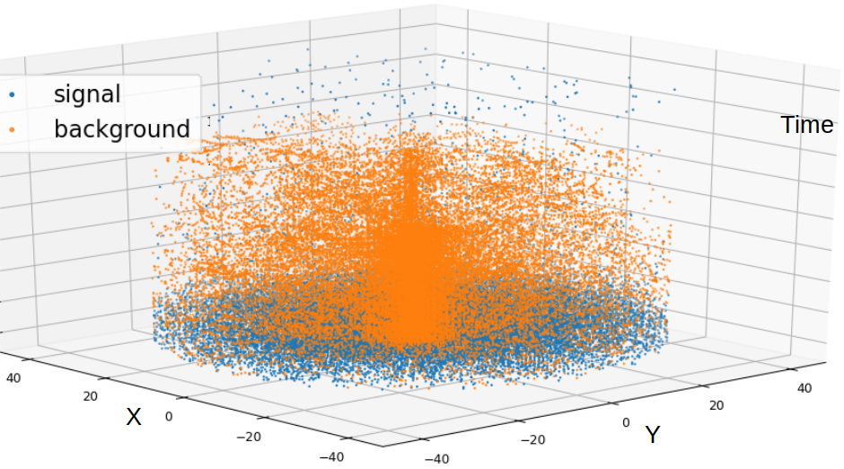
Figure 1: Feature space for the hits of about 400 Bhabha events. Noise hits (orange dots) happen uniformy over time.

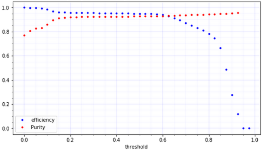
Figure 2: Purity and efficency of the results of the fully connected network versus threshold of probablity.

The model which works the best has seven fully connected hidden layers. This network can increase the original 70% average purity of the events to 93% and keep 94% of the signals [Fig. 2]. In other words, it removes 85% of the noise with the expense of losing about 6% of the signal hits. This result is the baseline for us to compare the effectiveness of other models, such as the CNN model introduced in the next section and the graph neural networks which will be presented in another article.

Since this model sees the hits one by one, we can apply it to one part of the data if needed. So it can be used in combination with other models. For example, in the next section, we show how to simplify the events to pictures with fewer resolutions. If we apply this dense model to the data lost during simplification, then the efficiency of the whole model is comparable to when no simplifications are involved, while it is a faster and lighter model in terms of memory use.

4 Convolutional neural networks

The 3D trajectory of particles in MDC lit the drift cells, which send their signals to the end caps at the ends of their lengths. Thus, our data in its raw format includes the 2D projection of the 3D events. The pixels of each image are arranged in 43 concentric circles, each with a different resolution. The number of cells gradually increases from 40 on the first two layers to 288 on the last three. There are several acceptable ways to map this to a square to feed the neural networks. Here, we choose a simple method of looking at the events with the resolution of the first layer. So, we map every event to a 2D image with a size of 43 by 40. This means that the information of some of the neighboring cells is combined at the outer layers.

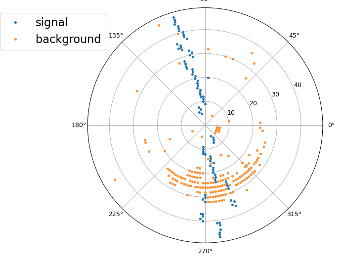
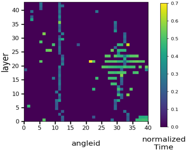
Figure 3: A sample event recorded at MDC is shown on the left side. The right side image shows the same event mapped on a 40 by 43 pixels image.

With this simplification, the neural network cannot make use of the information of about 2% of the hits. When that happens, one of the things that we can do is to just keep the hits that happened earlier since they are more likely to be signal hits. A better way is to pass that part of the hits from the classifying network introduced in the previous section. It was mentioned there that just looking at the time and position values of the hits can lead to more than 85% noise deletion and about 94% signal preservation. If we apply this to the 2%, this simplification of the images removes about 0.1% of the signal hits and pollutes the data for only about 0.2%. The real situation is even better since the hit classification results are more efficient better for the hits happening at the last layers. Therefore we take this simplification of the images as a good approximation. Furthermore, we normalize the time value of each hit and show it to the network just like color is presented for normal pictures (Fig. 3).

Our investigations show that a deep learning model with five convolutional layers and five dense layers can successfully remove noise hits while preserving signal tracks. This network does the job by detecting the tracks along with the use of time values. This situation is just like when the color of the pixels helps the segmentation process for regular images. We observe that it is necessary to downsize mildly with the filtering process of the convolutional layers, then flatten them and pass the results through dense layers. The last hidden layer has 64 nodes. The target layer has 1720 nodes which is the number of pixels needed to rebuild the pictures. It is not needed to have convolutional layers for upsampling which are present in models like Unet [3]. In the final image, the particle tracks are boldened, and the off-track noise is gone perfectly. Moreover, we test different thresholds to keep the hits. This way, the tracks become sharper, and the on-track noise also disappears. In the end, we intersect the result with the input to not have any extra hits. Figure 4 show the result of passing an event from the trained network and then applying the threshold.

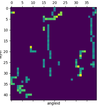
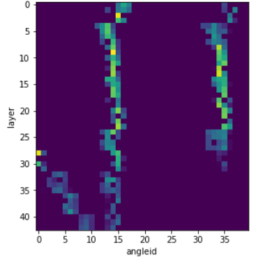
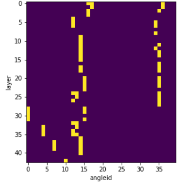
Figure 4: A random event which includes noise is shown on the left side. The image at the middle shows the outcome of the network for this image. The right side image shows the same result after applying a threshold.

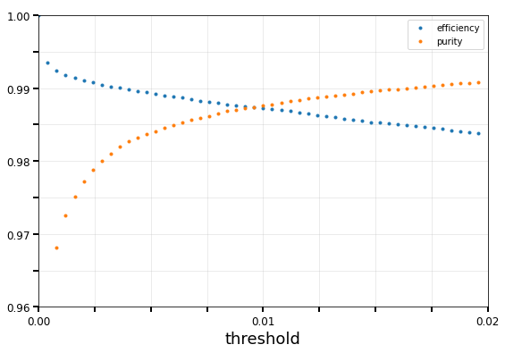
Figure 5: This diagram shows the average efficiency of the signal preservation and the average purity of the test events after they pass through the trained network.

We train the network with 77000 events up to about 100 epochs using the IHEP GPU farm. The result is an increase in the average purity of the events from the original amount of about 70% to 98% while about 99% of the signal hits are preserved (Fig. 5). This means that, on average, every event will have only about 1.5 noise hits and lose only one signal hit after passing through the trained network.

We examined many possibilities and came up with the above architecture of the convolutional network, which is a rich model with about 20 million trainable parameters. It is worth mentioning that for different purposes, different areas of Fig. 5 might be favorable. We usually use the crossing point of purity and efficiency diagrams to compare different models. After this work, we tried more complicated events and more detailed images, and it turned out that the same structure worked for them as well. As for the Bhabha events, we try 100 by 100 pixel images which have comparable resolution with the real 2D images, e.g. 6796 pixels. They also lead to similar results and show that the above model is acceptable. We will discuss them along with more techniques and results in an upcoming paper.

5 Concolusion

Since we already have many tools in high energy physics to generate simulated data and real data has also been stored for many years, it is very reasonable to use machine learning techniques in this area. Moreover, even a slight improvement in the purification of the stored events can be important in physics analysis. We see that even simplified models can have acceptable performances while being very fast and light which makes them good candidates for the trigger system or pre-processing of data. The hit classification approach for Bhabha events at the drift chamber of BESIII detector makes a baseline for further investigations. It also shows that a regression approach can be used in combination with other methods. Finally, the convolutional neural network that we introduced can distinguish the particle tracks and remove the noise in them in a way that the efficiency of the process and the purity of the final events are both about 98.7% at the same time.

References

References

- [1] M. Ablikim et al. Design and Construction of the BESIII Detector. Nucl. Instrum. Meth. A, 614:345–399, 2010.
- [2] Rong-Gang Ping. Event generators at BESIII. Chin. Phys. C, 32:599, 2008.
- [3] Olaf Ronneberger, Philipp Fischer, and Thomas Brox. U-net: Convolutional networks for biomedical image segmentation. In Medical Image Computing and Computer-Assisted Intervention – MICCAI 2015, pages 234–241, Cham, 2015. Springer International Publishing.