Hermes-3: Multi-component plasma simulations with BOUT++

Abstract

A new open source tool for fluid simulation of multi-component plasmas is presented, based on a flexible software design that is applicable to scientific simulations in a wide range of fields. This design enables the same code to be configured at run-time to solve systems of partial differential equations in 1D, 2D or 3D, either for transport (steady-state) or turbulent (time-evolving) problems, with an arbitrary number of ion and neutral species.

To demonstrate the capabilities of this tool, applications relevant to the boundary of tokamak plasmas are presented: 1D simulations of diveror plasmas evolving equations for all charge states of neon and deuterium; 2D transport simulations of tokamak equilibria in single-null X-point geometry with plasma ion and neutral atom species; and simulations of the time-dependent propagation of plasma filaments (blobs).

Hermes-3 is publicly available on Github under the GPL-3 open source license. The repository includes documentation and a suite of unit, integrated and convergence tests.

[llnl]organization=Lawrence Livermore National Laboratory, addressline=7000 East Avenue, city=Livermore, postcode=94550, state=CA, country=USA

[york]organization=School of Physics, Engineering and Technology, University of York, addressline=Heslington, city=York, postcode=YO10 5DD, country=UK

[ccfe]organization=United Kingdom Atomic Energy Authority, addressline=Culham Centre for Fusion Energy, Culham Science Centre, city=Abingdon, postcode=OX14 3DB, country=UK

PROGRAM SUMMARY

Program Title: Hermes-3
CPC Library link to program files:
Developer’s repository link: https://github.com/bendudson/hermes-3
Code Ocean capsule:
Licensing provisions: GPLv3
Programming language: C++14
Nature of problem: Simulation of dynamics and steady-state solutions of multiple ion and neutral species in magnetised plasmas using drift-reduced fluid plasma models in 1 to 3 spatial dimensions. Focused on but not restricted to the simulation of turbulence in the boundary of tokamaks.
Solution method: Hermes-3 implements a system of flexible software components, that are configured at run-time and coupled by passing a state object between them (the Encapsulate State and Command patterns). Hermes-3 builds on BOUT++ [1], employing the Method of Lines with implicit and explicit time-integration methods in curvilinear coordinates on block-structured meshes, making use of libraries including SUNDIALS, PETSc and Hypre. Hermes-3 implements drift-reduced plasma fluid equations using conservative finite difference methods, and atomic processes that couple plasma and neutral fluids.

1 Introduction

An important feature of magnetically confined fusion plasmas in tokamaks is that they consist of a mixture of different ion species. Computational studies of fusion plasma phenomena, such as plasma turbulence, have to date frequently treated plasmas as if they consisted of a single ion species, typically deuterium due to its use in experiments. In order to make predictions of phenomena important to the performance and design of the divertor of future fusion reactors, models must capture the interactions between plasma and neutral gas species (deuterium and tritium in a reactor), as well as radiation from impurity species (eg. Be, C, Ne, Ar, W), and pumping of helium “ash” and other species. In many cases none of these species can be treated as “trace” but are all coupled, so that all should be considered self-consistently in the same simulation. For each of these atomic species the density and dynamics of multiple states may need to be considered, for example the ground state, multiple ionisation stages, and molecular species. In some cases it may also be necessary to track metastable states, such as vibrationally excited states or charged molecules. The result is a potentially large number of species types which must be solved for, together with a complex set of reactions between them.

Historically there has been a division in terms of simulation tools and to an extent also research communities, between multi-fluid transport codes such as SOLPS [1], UEDGE [2], EDGE2D [3] and BOUT++/trans-neut [4], which employ simplified models for the cross-field transport (typically diffusive) but evolve many different species, and the turbulence codes including GBS [5, 6, 7], TOKAM3X [8, 9], (H)ESEL [10], and various models built on BOUT++ [11, 12, 13] such as Hermes [14] and STORM [15, 16]. These latter models can solve for the 3D time-varying turbulent transport, but typically only evolve a single ion species. During the last 5 years, and currently ongoing, are several efforts (e.g. [17, 18, 19]) to develop codes which can solve for the turbulent transport self consistently with multiple ion and neutral gas species [20].

If the number of species states to be solved for is relatively small, such as electrons, ions and a single atomic species as in Hermes-2 [21] and recent versions of STORM [16], then code can be written for each species. Unfortunately with this design the size of the code (number of lines) grows linearly with the number of species states, becoming increasingly error prone, difficult to test, and hard to maintain, as the number of species is increased. The authors’ experience with Hermes-2 indicated that this was not a viable path to multi-species simulations.

Here an open-source multi-fluid plasma simulation tool is presented, along with the flexible software design which makes the resulting model and software complexity manageable. It is built on BOUT++, which provides low-level data management and operations, and augments this with a reusable model component system. By doing this we unify 1D tokamak divertor simulation code SD1D [22] with 2D and 3D transport and turbulence code Hermes [14], and enable these tools to be extended towards multiple ion species simulations that self-consistently include both plasma turbulence and transport (atomic) physics.

In section 2 the numerical methods are described; in section 3 the software architecture is outlined and compared to prior work; and in section 4 a series of applications are presented, which demonstrate some of the capabilities of the new code. We conclude in section 5.

2 Numerical methods

In this section we describe the numerical methods used in Hermes-3 components. The architecture described in section 3.2 does not enforce the choice of numerical method, but this section describes the methods that have been implemented to date and are used in section 4. The system of PDEs is solved using the method of lines, in which the time and spatial dimensions are treated separately: The time integrator simply integrates a set of Ordinary Differential Equations (ODEs), and is discussed in section 2.1; The spatial discretisation is by finite difference methods (section 2.2). Boundary conditions are discussed in section 2.3.

2.1 Time integration

Hermes-3 is built on the BOUT++ framework [13], and so can make use of a range of explicit (e.g RK4), fully implicit (e.g. BDF via SUNDIALS [23]), and implicit-explicit (e.g IMEX-BDF2 and ARKODE via SUNDIALS) methods. These were implemented with the aim of studying time-dependent problems, such as the study of Edge Localised Mode (ELM) eruptions [24] or tokamak edge turbulence [25], where accurate time evolution is required.

Many of the problems of interest for Hermes-3 are steady state: Axisymmetric tokamak transport solutions, potentially as a starting point for 3D time-dependent turbulence simulations. To find these steady-state solutions efficiently it is desirable to take large timesteps, ideally an infinite timestep, damping transient oscillations in the system. A dissipative time integration scheme that is unconditionally stable is therefore desirable. A first order backward Euler method and preconditioning algorithm similar to that used in UEDGE [2] has been implemented here. This method is stable for any timestep provided that the nonlinear solver, typically a variety of Newton’s method, iterations converge. In practice this limits the timestep to a finite, and sometimes quite small, value.

An important ingredient to robustly and efficiently solving the nonlinear problem at each time step is a good preconditioner: It enables the linear inner solve to converge with fewer iterations (and so computational cost) for larger timesteps than would otherwise be possible. Custom preconditioners developed using a methodology such as physics-based preconditioning [26, 27] can be highly effective, but are challenging in multi-fluid contexts: The tokamak edge is a highly nonlinear system, with a potentially large number of species (and so equations), coupled through atomic rates which are typically tabulated rather than analytic, and which vary by orders of magnitude over relatively small temperature ranges. The approach used in UEDGE, and adopted for the Backward Euler solver here, is to use finite differences to calculate the elements of the system Jacobian $\mathbb{J}_{ij}=\frac{\partial}{\partial f_{j}}\frac{\partial f_{i}}{\partial t}$ where $\mathbf{f}$ is the vector of evolving quantites. This approximate Jacobian is used to construct a preconditioner that (approximately) solves the linear operator $\mathbb{I}-\Delta t\mathbb{J}$ for timestep $\Delta t$. Methods based on incomplete LU factorization (ILU) have been found to be effective: In serial the PETSc ILU(k) solver is used, and in parallel the Euler library [28] within hypre [29], both with default settings.

The calculation of a dense Jacobian using finite differences would be prohibitively slow in most cases: A typical simulation might contain $N\simeq 10^{5}-10^{8}$ evolving quantities, while the Jacobian has $N^{2}$ elements. Fortunately the Jacobian is typically sparse, because the finite differences and other interaction terms are local. This is exploited by using the PETSc coloring facilities [30], which are provided with the matrix structure (determined by the finite difference stencil), and efficiently calculate many Jacobian matrix entries simultaneously. Because each cell only has a fixed number of neighbours, the cost of evaluating the Jacobian is reduced from scaling like $N^{2}$ to scaling approximately linearly with the number of grid cells $N$.

The effectiveness of this time integrator for steady state problems will be applied to 1D transport problems in section 4.1 (fig 5), and for 2D transport in an axisymmetric tokamak geometry in section 4.2.

2.2 Finite differencing spatial operators

The models to be shown here use conservative finite difference operators that were implemented in the Hermes code [14] and have been improved over time and moved into the BOUT++ library. All quantities are cell centred, and advection operators are written in terms of fluxes between cells calculated at cell faces. The cross-field operators presently assume that the grid is orthogonal in the tokamak poloidal plane. This limits the accuracy with which strongly shaped divertor geometries can be simulated with the present code. Non-orthogonal grids which align with wall surfaces can be generated for Hermes using the BOUT++ grid generator [31], but the required off-diagonal metric terms have not yet been implemented. Those terms have long been implemented in UEDGE, and were recently added to SOLPS [32], where they were found to be essential for fluid neutral modelling on distorted grids, but relatively unimportant when kinetic neutrals were used. Implementing these terms is a high priority for future improvements to Hermes-3.

Because all quantities are cell centred, in the absence of dissipation zig-zag modes are likely to develop. In [14] an Added Dissipation [33] artificial dissipation term was used in advection operators along the magnetic field. Here this is replaced with an HLL type flux splitting method [34, 35], that improves on methods used previously for 1D tokamak divertor simulations [22, 36]. Results shown here use either the MinMod or Monotonised Central (MC) slope limiters [37], that have been found to provide a good balance of numerical dissipation and stability. Details of the method are given in A.

To verify the implementation of fluid flow along the magnetic field for smooth solutions, a set of 1D fluid equations along a magnetic field given in equation 1 is tested using the Method of Manufactured solutions (MMS). This testing method has become widely used to verify the correct implementation of complex sets of equations, in tokamak edge plasma codes [38] including BOUT++ [39].

$$\frac{\partial n}{\partial t} =-\nabla\cdot\left(n\mathbf{b}v_{||}\right)$$ (1a)

$$\frac{\partial p}{\partial t} =-\nabla\cdot\left(p\mathbf{b}v_{||}\right)-\frac{2}{3}p\nabla\cdot\left(\mathbf{b}v_{||}\right)$$ (1b)

$$\frac{\partial}{\partial t}\left(mnv_{||}\right) =-\nabla\cdot\left(mnv_{||}\mathbf{b}v_{||}\right)-\partial_{||}p$$ (1c)

Error norms as a function of mesh cell spacing are presented in figure 1, showing convergence towards the manufactured solution on a 1D periodic domain. Second order convergence is found for both $l_{2}$ and $l_{\infty}$ error norms, consistent with the expected order of accuracy of the numerical methods.

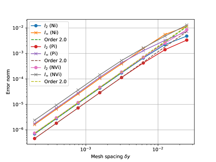
Figure 1: Verification of the convergence of a 1D system of fluid equations on a periodic domain. Showing $l_{2}$ (Root-Mean-Square) and $l_{\infty}$ (Max) errors for the evolving density $N_{i}$, pressure $P_{i}$ and momentum $NV_{i}$. Figure produced by tests/integrated/1D-fluid in the Hermes-3 repository [40].

The intended application of Hermes-3 is to magnetically confined fusion plasmas, in which flows are typically subsonic. Nevertheless the code must be robust to transients, and transitions to supersonic flow can occur in tokamak plasmas [41]. Figure 2 shows the results of the standard 1D Sod shock tube test case [42].

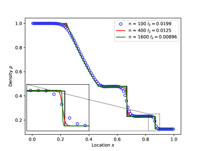
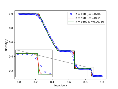
Figure 2: Standard Sod shock tube problem [42] at $t=0.2$, with exact (analytic) solution in solid black. A solution with reference resolution ($n=100$ cells) is compared to higher resolutions and their $l_{2}$ (Root-Mean-Square) errors. Left: Solving the pressure form of the fluid equations. Right: Solving the energy form. The inset figures show the shock front in more detail. Figure produced by tests/integrated/sod-shock and tests/integrated/sod-shock-energy.

In the expanded view shown inset in the left figure 2 it can be seen that the numerical shock location lags the exact solution, so that the $l^{2}$ error norm does not converge to zero. The result is insensitive to time integration method, being observed with both the default CVODE time integrator and the RK3-SSP method implemented in BOUT++. This is due to the choice of pressure as an evolving quantity in equation 1, and so pressure fluxes are calculated at cell edges.

Hermes-3 is structured in a modular way that allows equations to be changed in the input file. If rather than evolving pressure we choose to evolve energy density $\mathcal{E}=\frac{3}{2}p+\frac{1}{2}mnv_{||}^{2}$, then the result is shown on the right of figure 2. Solving the fluid equations in this conservative form recovers the correct shock front location (shown inset in figure 2 right). Further variations on this 1D shock tube problem [43] are included in the Hermes-3 test suite.

We conclude that the methods currently implemented are $2^{nd}$-order accurate for smooth solutions (figure 1), and remain robust around shocks, contact discontinuities and expansion waves (figure 2). The modular nature of Hermes-3 allows multiple fluid formulations to be implemented and inter-operate to suit different applications.

2.3 Boundary conditions

The domain typically solved for in 2D and 3D Hermes-3 tokamak simulations is an annulus consisting of a region of closed and open magnetic flux surfaces. An example is discussed in section 4.2 and shown in figure 8. The hot “core” of the plasma is not modelled because the fluid equations solved become invalid in that region. Instead a boundary condition must be imposed at that innermost surface where no boundary physically exists. At the outer edge of the domain the grid is typically close to, but not aligned with, the solid vacuum vessel of the tokamak. Boundary conditions for the thermodynamic variables on both “core” and “wall” boundaries are typically set to either Dirichlet or Neumann.

The boundary condition on the potential $\phi$ is a variation on the method used in the STORM model [16, 15]: A time-evolving boundary condition that relaxes towards a Neumann boundary. This is implemented in the following way: When inverting the Laplacian-type equation for $\phi$ from vorticity, the potential is fixed at both core and wall boundaries. If a simple Dirichlet condition is used then narrow boundary layers typically form close to the boundaries in which the imposed boundary potential is matched to the plasma potential. These boundary layers can develop unphysical instabilities. Instead, at every timestep the value of the boundary condition is adjusted towards the value inside the domain with a characteristic timescale that is set by default to $1\mu s$. In this manner the electrostatic potential $\phi$ evolves smoothly to solutions that can have different potentials on core and wall boundaries.

3 Software architecture

Hermes-3 [40, 44] aims to support a wide range of different models, with an arbitrary number of species and equations. This flexibility presents a challenge for the software design: A poorly chosen architecture will result in the code complexity growing rapidly with the model size, so that further progress becomes increasingly difficult as the model is extended.

There are many domains besides tokamak plasma physics where performance is important, and where many different software components have to interact in complex ways which need to be extended over time as the software grows and is applied to new problems. A variety of approaches have been developed within scientific computing and in other fields. In section 3.1 we briefly describe some of the approaches that influenced the design of Hermes-3.

3.1 A brief survey of approaches

Within physical sciences there are a number of codes which have adopted designs that enable users and developers to develop components or plugins, and to combine them in novel ways so that the ecosystem becomes increasingly useful as new components are added. An example is LAMMPS [45], which uses a system of “styles” that define interfaces which users can implement to modify the simulation behaviour.

In the software industry Entity Component Systems (ECS) are a design pattern which is commonly used in game development. Those are intended to describe a set of “Entities” that have defined sets of behaviour and can interact with each other. This design pattern offers flexibility through composition rather than inheritance, and considerable run-time configurability. A widely used and high-performance implementation of an ECS is EnTT [46].

Task graphs are another widely applicable and powerful approach to thinking about computations, which focuses on managing the dependencies between components, so that at a high level the whole calculation is a directed acyclic graph (DAG). Examples of task-based systems include StarPU [47] and TaskFlow[48].

An important aspect of all of these approaches is splitting complex models into simpler components, which interact through standardised interfaces and not global state. This facilitates testing, in particular unit testing, provides a powerful way to mitigate the growth of complexity, and helps to maintain productivity as code becomes larger.

3.2 The design of Hermes-3

The design of Hermes-3 is a combination of the Encapsulate Context [49] and Command patterns [50]. The main elements are a flexible store or database, into which values (e.g. spatially dependent fields like densities, temperatures) can be inserted and later retrieved; and a collection of composable model components that set and use values in the store. The approach has similarities to data oriented design [51], in which loose coupling between components is achieved by focusing on defining the data being operated on. In fusion an example of this is the OMFIT framework [52], which uses a tree data structure to loosely couple data sources, codes and analysis scripts.

The data in a simulation is physical quantities, such as density and temperature fields, and derived quantities representing terms in the equations being solved. Hermes-3 stores these quantities in a nested dictionary structure (a tree), using C++ variant to enable different data types to be stored. A schema defines a convention for where values are stored, for example state["species"]["h+"]["density"] is the number density of hydrogen ions.

Operations on the simulation state are performed by a collection of composable model components, that set and use values in the state. For example there is a component that evolves an equation for fluid number density, another component that evolves pressure. These components are configured when they are created, so that the same code is used to evolve every species that needs that component. Every component can access the whole state, so some perform calculations for a single species, while others perform calculations involving multiple species (e.g. collisions, sheath boundary conditions).

An important distinction between this design and one with a shared global state is that here the state is an object which is passed to components in a user-defined order. This has two advantages: It controls when state can be modified, making the flow of the program easier to understand, and it facilitates unit testing because the inputs to the components can be precisely specified with no hidden side-channels or large setup/teardown procedures.

Controlling when and how data can be modified is crucial to preventing errors, such as components being run out of order so that quantities are set or modified after use. The values being calculated are physical quantities at the current simulation time, and so logically do not change. It is therefore tempting to adopt an immutable (persistent) data structure, such as the HAMT used in Clojure [53] and available in C++ libraries such as Immer [54]. There are however situations in which components need to modify fields set by earlier components; an important example is applying boundary conditions. Rather than copy arrays of data to maintain immutability, the approach used here is to mark quantities as immutable after they have been used: A quantity can be modified (e.g. boundary conditions applied) only if that quantity has not already been used in a previous calculation.

The flow of information carried by the state through a sequence of components is shown in figure 3.

Figure 3: The State of the simulation system is passed through a sequence of Components in two passes. In the first pass components can modify the state passed to their transform function; in the second pass the state cannot be modified, but is used to update component internal states in their finally functions.

This design restricts when the state can be modified, limiting the complexity of interactions between components, and making the logic of the program easier to follow. In Hermes-3 the state is passed to each component twice: The first time the state is mutable, and the component can insert values into it. After all components have been called in this way, the state is “frozen”, and passed to each component again but cannot be modified. In this second pass each component can use the final state to update its own internal state, such as time derivatives to be passed to the time integrator. This means that components can depend on each other’s outputs, including mutual dependencies, but all modifications must be in the first function (called transform()), and in the second function (called finally()) all components can assume that the state will not subsequently change. This structure could be exploited to enable all component finally() functions to be run in parallel, but this is not currently done in Hermes-3.

The design of Hermes-3 enables run-time configuration of the simulation equations: All of the examples shown in section 4 use the same executable, despite solving different sets of equations in different numbers of spatial dimensions. The overhead of this flexibility appears to be small, but for high performance scientific simulation codes it is debatable whether run-time configuration is essential: Once the simulation is set up, it is performing the same set of operations repeatedly, calculating time derivatives given different system states. Run-time configuration enables the user (scientist) to modify the equations without recompiling, but means that some errors are only caught at runtime, which might have been caught more quickly at compile time. Compile-time configuration of the equations solved might enable more optimisations, since conditionals can be known and optimised out by the compiler. Just-In-Time (JIT) compilation might offer the best of both worlds; since the operations are the same with different data, run-time analysis of the performance might enable on-the-fly tuning to identify bottlenecks and optimise throughput.

4 Applications

We now describe some applications of Hermes-3, starting from a 1D transport model (section 4.1); then a 2D transport model in 2D (axisymmetric) tokamak geometry (section 4.2). Finally we demonstrate time-dependent capabilities by simulating 2D (drift plane) plasma “blobs” (section 4.3). Application of these capabilities to 3D turbulence simulations is relatively straightforward, but requires significantly more space to describe adequately and so will be explored in separate publications.

4.1 1D transport

We first apply Hermes-3 to a one-dimensional problem: the flow of heat and particles along a magnetic flux tube which is in contact with a material surface. The model includes electrons, deuterium ions and neutral deuterium atoms. One end of the domain is modelled as being in contact with a material surface, forming a plasma sheath and accelerating ions to the sound speed. The flow of ions to the surface is “recycled” back into the domain as neutral atoms, which then undergo charge exchange and ionisation reactions with the plasma. The other end of the domain has a symmetry (no-flow) boundary condition, where thermodynamic variables (e.g. densities, pressures) have zero gradient, and flow velocities are zero. This is a widely used model for the divertor region of tokamak plasmas, which has several implementations of varying complexity [55, 56, 57, 58, 59, 60], including the SD1D model [22, 36] which like Hermes-3 is built on BOUT++ [12].

Despite its relative simplicity this model contains many of the nonlinearities and numerically stiff behaviour which make 2D and 3D plasma simulations challenging, including strong nonlinear heat diffusion, and fast reaction rates which are sensitive to electron temperature.

The components to be included in the simulation (section 3.2) are specified in an input text file; the relevant line is shown in listing 1.

⬇

1[hermes]

2components = (d+, d, e,

3 sheath_boundary, collisions, recycling, reactions,

4 electron_force_balance, neutral_parallel_diffusion)

Listing 1: Top-level components for 1D hydrogen transport model. Parentheses are used to group multi-line settings. Full input in examples/1D-recycling of the Hermes-3 repository [40]

The boundary condition at the material surface, implemented by the sheath_boundary component in listing 1, is the multi-ion sheath boundary described in [61]. For the single ion species here this reduces to the standard Bohm-Chodura-Riemann sheath boundary condition [62]. The collisions component implements collisions between an arbitrary number of charged and neutral species. Reactions between species are organised into a subsection called reactions, and are chosen to have names which are readable and follow a convention for the species labels.

⬇

1[reactions]

2type = (

3 d + e -> d+ + 2e, # Deuterium ionisation

4 d+ + e -> d, # Deuterium recombination

5 d + d+ -> d+ + d, # Charge exchange

6 )

Listing 2: Reactions contained in the 1D hydrogen transport model

Reaction cross-sections for hydrogen and helium have been taken from the Amjuel database [63].

Each particle species has components to evolve the density, pressure and parallel momentum, and a no-flow boundary condition imposed on the upstream boundary. To illustrate how Hermes-3 components combine to form the equations solved, the d+ (deuterium ion) species settings are shown in listing 3.

⬇

1[d+] # Deuterium ions

2type = (evolve_density, evolve_pressure, evolve_momentum,

3 noflow_boundary, upstream_density_feedback)

4charge = 1 # charge

5AA = 2 # mass [amu]

6density_upstream = 1e19 # Upstream density [m^-3]

7recycle_as = d # Species to recycle as

8recycle_multiplier = 1 # Recycling fraction

Listing 3: Components to model the deuterium ion species

This implements a set of equations for the density $n_{d+}$, pressure $p_{d+}=en_{d+}T_{d+}$ and parallel velocity $v_{||d+}$ of the deuterium ions (d+) of mass $m_{d+}$ and charge $q_{d+}$, given in equation 2. These equations are in SI units except temperatures in eV.

$$\frac{\partial n_{d+}}{\partial t} =-\nabla\cdot\left(n_{d+}\mathbf{b}v_{||d+}\right)$$

$$+\underbrace{S_{\textrm{PI}}}_{\texttt{upstream\_density\_feedback}}+\underbrace{n_{e}n_{d}\left<\sigma v\right>_{iz}}_{\texttt{d + e -> d+ + 2e}}-\underbrace{n_{e}n_{d+}\left<\sigma v\right>_{rc}}_{\texttt{d+ + e -> d}}$$ (2a)

$$\frac{\partial p_{d+}}{\partial t} =-\nabla\cdot\left(p_{d+}\mathbf{b}v_{||d+}\right)-\frac{2}{3}p_{d+}\nabla\cdot\left(\mathbf{b}v_{||d+}\right)+\nabla\cdot\left(\kappa_{||d+}\mathbf{b}\mathbf{b}\cdot\nabla T_{d+}\right)$$

$$+\underbrace{n_{e}n_{d}\left<\sigma v\right>_{iz}\left[eT_{d}+\frac{1}{2}m_{d}\left(v_{||,d}-v_{||,d+}\right)^{2}\right]}_{\texttt{d + e -> d+ + 2e}}$$

$$+\underbrace{n_{d+}n_{d}\left<\sigma v\right>_{cx}\left[e\left(T_{d}-T_{d+}\right)+\frac{1}{2}m_{d}\left(v_{||,d}-v_{||,d+}\right)^{2}\right]}_{\texttt{d + d+ -> d+ + d}}$$

$$-\underbrace{n_{e}n_{d+}\left<\sigma v\right>_{rc}eT_{d+}}_{\texttt{d+ + e -> d}}+\underbrace{W_{d+}}_{\texttt{collisions}}$$ (2b)

$$\frac{\partial}{\partial t}\left(m_{d+}n_{d+}v_{||d+}\right) =-\nabla\cdot\left(m_{d+}n_{d+}v_{||d+}\mathbf{b}v_{||d+}\right)-\mathbf{b}\cdot\nabla p_{d+}+q_{d+}n_{d+}E_{||}$$

$$+\underbrace{n_{e}n_{d}\left<\sigma v\right>_{iz}m_{d}v_{||d}}_{\texttt{d + e -> d+ + 2e}}-\underbrace{n_{e}n_{d+}\left<\sigma v\right>_{rc}m_{d+}v_{||d+}}_{\texttt{d+ + e -> d}}$$ (2c)

$$+\underbrace{n_{d+}n_{d}\left<\sigma v\right>_{cx}m_{d+}\left(v_{||d}-v_{||d+}\right)}_{\texttt{d + d+ -> d+ + d}}+\underbrace{F_{d+}}_{\texttt{collisions}}$$ (2d)

Where $\mathbf{b}\equiv\mathbf{B}/B$ is the unit vector in the direction of the magnetic field $\mathbf{B}$, and $\kappa_{||d+}$ is the parallel heat conduction coefficient that depends on the collision frequency calculated by the collisions component. For each equation 2 the first line corresponds to the essential transport terms implemented in the evolve_density, evolve_momentum and evolve_pressure components. Additional components, labelled with underbraces in equation 2, add sources and sinks that modify and couple species together. Details of the full system of 7 evolving equations are given in B.

The equations are integrated in time towards a steady state solution using the backward Euler method described in section 2.1. The result is shown in figure 4.

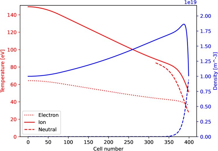
Figure 4: Steady-state solution to system of equations 2 and B in one dimension. 50MW of power enters a source region on the left, driving plasma-neutral interactions including ionisation, leaving through the sheath boundary on the right. 100% of the plasma ions leaving the right boundary are recycled as neutral atoms. Simulation inputs are in examples/1D-recycling in the Hermes-3 repository.

The root-mean-square of the time-derivatives of ion density, pressure and parallel momentum are shown in figure 5 as a function of the number of right-hand-side (RHS) evaluations, a measure of the computational cost. This evaluation count includes those performed as part of the finite difference Jacobian approximation. This shows a reduction in the time derivatives of the system by almost six orders of magnitude in $10^{5}$ RHS evaluations. For the above system of equations, with 400 grid cells, this calculation takes approximately 30 minutes on a single core.

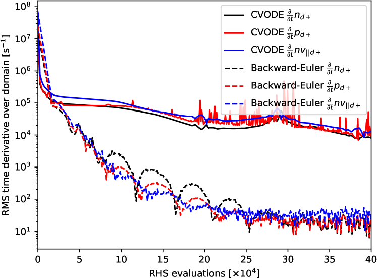
Figure 5: Root-mean-square time derivatives of deuterium density (Nd+), pressure (Pd+) and momentum (NVd+) as a function of iteration (RHS evaluation). These converge towards zero as the system approaches steady state. Results are shown for Backward Euler Newton-Krylov with Jacobian coloring and iLU preconditioning (NK); and the CVODE time integrator. Figure produced by examples/1D-recycling/plot_convergence.py.

For comparison the convergence towards steady state with the Sundials CVODE [23] library is shown in figure 5. CVODE uses an adaptive order, adaptive timestep Backward Differentiation Formula (BDF) method, and is highly effective for time-dependent problems of interest even without preconditioning (e.g. the plasma blobs application, section 4.3). For this problem only the parallel heat conduction is preconditioned. Figure 5 shows that the Backwards-Euler with Jacobian coloring preconditioner method can provide significantly better performance for steady-state problems, though it would not be a good choice for time-dependent simulations, being only first order accurate in time.

In this simulation the recycling at the “target” end of the domain was set to 100%, while there is a no-flow condition on the upstream boundary. A Proportional-Integral (PI) controller is used to control an upstream particle source (implemented in the upstream_density_feedback component); As the target upstream density is approached, this input source should go to zero if mass flow is conserved. Figure 6 shows that this does indeed happen: The source converges towards exponentially towards zero in steady state.

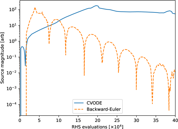
Figure 6: Convergence of the density source with RHS evaluation in a 1D simulation with 100% recycling (figure 4) where the true steady state source is zero. Figure produced by examples/1D-recycling/plot_convergence.py.

The 1D simulation described here is a useful tool in its own right, for studies of plasma dynamics and detachment in magnetised plasmas. The advantage of the software design used in Hermes-3 (section 3) is that the same code can extend to more complex models and higher dimensions with only changes to the input.

4.1.1 Impurity seeding

We now extend the 1D simulation described in section 4.1 to multiple ion species, by including all ten charge states of neon as separate species. The simulation now contains 40 evolving fields: The density, pressure and momentum of all deuterium and neon ion and atomic charge states (13 ion species in total), and the electron pressure. These species are coupled through collisions, thermal forces, the parallel electric field, and 32 atomic reactions: ionisation, 3-body recombination and charge exchange recombination (with deuterium ions) of each ionisation level of neon; ionisation and charge exchange of neutral deuterium atoms to deuterium ions. The modular structure of the code (section 3.2) enables this to be accomplished relatively straightforwardly by changing the input file.

⬇

1[hermes]

2components = (d+, d, ne, ne+, ne+2, ne+3, ne+4, ne+5, ne+6,

3 ne+7, ne+8, ne+9, ne+10, e, sheath_boundary,

4 thermal_force, collisions, recycling, reactions,

5 electron_force_balance, neutral_parallel_diffusion)

Listing 4: Top-level components for 1D transport model with neon. Input examples/1D-neon

There are now many more reactions, but the input remains clear:

⬇

1[reactions]

2type = (

3 d + e -> d+ + 2e, # Deuterium ionisation

4 d + d+ -> d+ + d, # Charge exchange

5

6 ne + e -> ne+ + 2e, # Neon ionisation

7 ne+ + e -> ne, # Neon+ recombination

8 ne+ + d -> ne + d+, # Neon+ charge exchange recombination

9

10 ...

11 )

Listing 5: Reactions contained in the 1D transport model with neon.

The cross-sections and radiated power from the neon reactions are calculated using ADAS [64]: scd96 and plt96 for ionisation; acd96 and prb96 for recombination; ccd89 for charge exchange. These files were converted to JSON format using atomic++ [65].

Collisions and the thermal forces between species are calculated as described in section 4.1. Those Braginskii energy and momentum exchange rates are approximations which are only strictly valid when heavy ions are trace impurities. In the simulations shown here the neon concentration is small (a fraction of a percent). More complete models of collisions in a multi-ion plasma have been derived [66] and recently generalised [67]. Implementing these models into Hermes-3 is left as future work, but is not anticipated to present any fundamental difficulty.

Starting from the hydrogen simulation described above (section 4.1), a simulation with 100% recycling and an initial uniform low concentration of neon is run to steady state, and shown in figure 7. In this simulation there is no net flow upstream of the ionisation region, and so thermal forces drive neon impurities upstream.

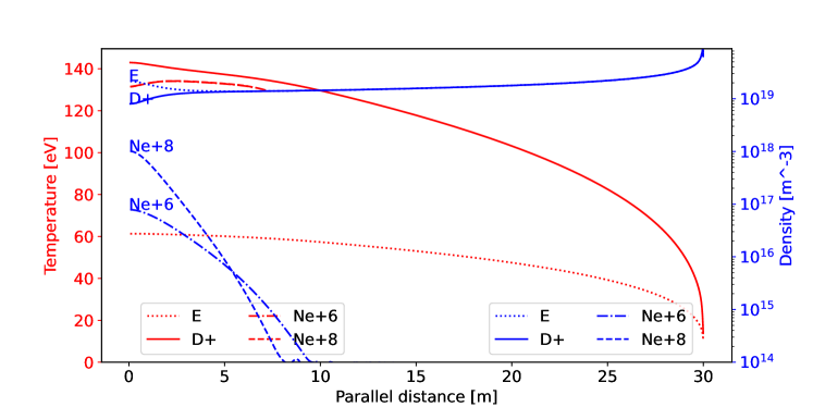
Figure 7: Steady state solution with 100% recycling, evolving all charge states of neon as separate fluids with their own densities, temperatures and flow velocities. A subset of species densities (blue lines) are shown on a logarithmic scale. Simulation inputs in examples/1D-neon of the Hermes-3 repository.

The steady-state solution is shown in figure 7. Future applications of this capabilty include simulating impurity-seeded plasma detachment phenomena.

4.2 2D (axisymmetric) transport

The same code that is used in a 1D domain in the previous sections can be applied to 2D tokamak domains with one or two X-points. By introducing cross-field diffusion of both charged and neutral species, an axisymmetric tokamak transport simulation in the spirit of SOLPS [1], EDGE2D [3] or UEDGE [2] can be performed, though not yet at a comparable level of maturity or completeness. To demonstrate the ability of Hermes-3 to solve axisymmetric transport problems, simulations are performed with deuterium ions and neutral atoms. Diffusion coefficients and plasma parameters are taken from [68, 69]: Spatially constant cross-field diffusion coefficients for particle transport $D_{n}=0.15$m${}^{2}/$s, electron and ion thermal transport $\chi_{e}=\chi_{i}=4$m${}^{2}/$s. In general these coefficients can be functions of location, and can be different for each species.

The plasma equilibrium is based on a COMPASS-like equilibrium generated using analytic Grad-Shafranov solutions [70, 71]. The domain simulated is shown in figure 8, consisting of a narrow annulus around the separatrix (dashed black lines in figure 8) including closed and open field line regions. The radial boundaries are at normalised poloidal flux ($\psi_{N}$) of 0.9 in the core and in the private flux region (PFR), and 1.3 in the Scrape-Off Layer (SOL). The Hypnotoad tool [31] was used to generate a sequence of grids of increasing resolution from $16\times 24$ to $64\times 96$ (radial $\times$ poloidal cells).

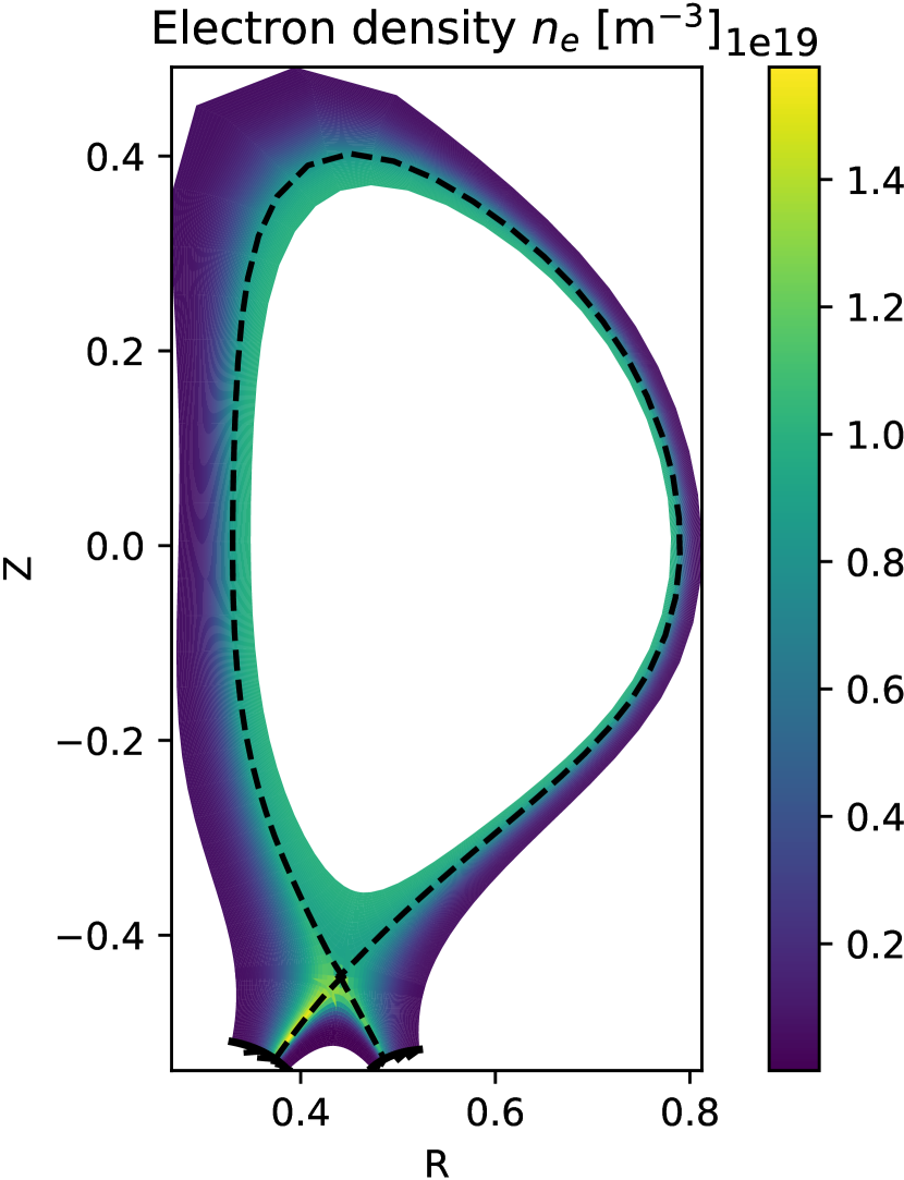
(a) Electron density. The core boundary is fixed to a density of $1\times 10^{19}$m^-3. At divertor targets 99% of ion flux is recycled as neutral atoms.

(b) Electron temperature. At the core boundary both electron and ion temperatures are fixed to $75$eV.

Figure 8: Axisymmetric tokamak transport simulation of deuterium ions and atoms. Equations given in B. Simulation inputs in examples/tokamak/recycling of the Hermes-3 repository.

As in previous examples, the equations solved are specified as a set of components:

⬇

1components = (d+, d, e,

2 collisions, sheath_boundary_simple,

3 recycling, sound_speed, reactions,

4 electron_force_balance)

Listing 6: Top-level components for 2D transport model. Full input in examples/tokamak/recycling of the Hermes-3 repository.

The deuterium ion species is configured with a set of components representing the equations solved, given in listing 7

⬇

1[d+]

2type = (evolve_density, evolve_momentum, evolve_pressure,

3 anomalous_diffusion)

4anomalous_D = 0.15 # Density diffusion [m^2/s]

5anomalous_chi = 4 # Thermal diffusion [m^2/s]

6...

Listing 7: Deuterium ion components for 2D transport model

which is similar to the configuration in 1D simulations given in listing 3, but adds anomalous cross-field diffusion terms. Reactions between species are calculated using Amjuel rates [63], comprising ionisation, recombination, and charge exchange processes as described in section 4.1.

At the inner (core) boundary the deuterium density is fixed to $1\times 10^{19}$m^-3; electron and ion temperatures are set to $75$eV. This core boundary therefore acts as a source of heat and particles. At the target plates a sheath boundary condition is applied in which the plasma flow goes to the sound speed, with a recycling fraction of 0.99 so that there is a flux of neutral atoms into the domain at the target plates. The 1% of ion flux that is not recycled is balanced in steady state by a diffusion of ions from the core boundary. This particle flux balance will be used in section 4.2.2 to verify the conservation of particles in these simulations.

The heat flux along the magnetic field into the target plates is given by $q_{||e,i}=\gamma_{e,i}neTc_{s}$ with sheath heat transmission factors $\gamma_{e}=4.8$ for electrons and $\gamma_{i}=3.5$ for ions. The sound speed into the sheath is $c_{s}=\sqrt{e\left(T_{i}+T_{e}\right)/m_{i}}$. There are no diffusive fluxes to the outer walls because zero-gradient boundary conditions are used there. The power into the target plates should therefore equal the input power through the core boundary, less the power radiated during atomic processes (primarily ionisation). This is used in section 4.2.2 to assess conservation of energy.

The full set of equations solved are given in B.

4.2.1 Evolution to steady state

The system of transport equations is relatively small (e.g. 10,752 variables for the $32\times 48$ mesh) but highly nonlinear and with a wide range of timescales, making finding steady state solutions challenging. Simple application of a nonlinear solver does not converge in most cases of interest, and the system must be regularised using a (pseudo-)timestepping approach. As the system approaches steady state the timestep can be made progressively larger, usually in an automated manner based on the number of nonlinear iterations required to converge the previous step. The combination of time integration method, time step adjustment heuristic, nonlinear solver, inner linear iterative solver, and preconditioner have many parameters that can affect performance. The nested methods interact in ways that are problem-dependent, making general conclusions regarding performance difficult to draw. The performance results presented here (e.g. figure 9) should therefore be taken as somewhat anecdotal, the important aspects being the energy and particle conservation properties (table 1) and scaling with problem size.

In general power balance reaches steady-state on a shorter timescale than the particle balance: The thermal energy content of the system (plasma + neutrals) is $W\simeq 47$J, so the energy confinement time is $\tau_{E}\equiv W/P_{in}\simeq 0.24$ms. On the other hand the ion particle content is approximately $2\times 10^{18}$, giving a particle throughput timescale of $\tau_{p}\simeq 45$ms. This longer particle balance timescale becomes increasingly challenging at high recycling fractions relevant to large fusion devices.

An effective strategy, already used routinely and interactively in UEDGE, is progressive mesh refinement: Starting on the coarsest mesh ($16\times 24$ here), CVODE is used with an absolute tolerance of $10^{-12}$ and relative tolerance $10^{-5}$, tightening the relative tolerance to $10^{-8}$ as steady state is approached. These tolerances can be loosened in some cases, but at the risk of numerical instability and convergence failure after a number of steps. Once progress has been made on a coarse mesh, the solution is interpolated onto a higher resolution mesh (using SciPy’s RegularGridInterpolator [72] over logically rectangular mesh patches). The simulation is then continued using an increased number of cores. The refinement process may be repeated. Figure 9 shows the Root-Mean-Square (RMS) of the time derivatives of the plasma density averaged over the domain, as a function of wall clock time (running on NERSC’s Perlmutter).

(a) CVODE solver with heat conduction preconditioner

(b) Backward Euler solver with PETSc matrix coloring and Hypre’s Euler preconditioner

Figure 9: Evolution of the Root-Mean-Square (RMS) time derivative residuals. Vertical red arrows indicate where the solution is interpolated onto a higher resolution mesh. Blue stars are the solutions that are compared in section 4.2.2. The number of cores used is increased with the grid resolution: $12$ ($16\times 24$ mesh), $48$ ($32\times 48$ mesh) and $192$ ($64\times 96$ mesh).

For each mesh resolution the simulation was continued after interpolation, until the Root-Mean-Square time scale exceeded one second, to minimise the impact of mesh interpolation error on the comparison of solutions. As the mesh was refined the number of cores used was increased following a weak scaling. The increase in run time with grid resolution in figure 9 is primarily driven by the number of iterations required: For CVODE the iteration counts are $3.1\times 10^{6}$ ($16\times 24$ mesh), $1.2\times 10^{7}$ ($32\times 48$ mesh) and $3.7\times 10^{7}$ ($64\times 96$ mesh). The time per iteration (RHS evaluation) is 1.7ms, 2.0ms and 4.3ms respectively.

Figure 9(b) shows results using the Backward Euler method with Jacobian coloring and Euler ILU preconditioner that was described in section 2.1 and used in 1D simulations (section 4.1). In general a significant improvement in performance is found, primarily due to a reduction in the number of iterations required. The speedup is most significant for small meshes and processor counts, where direct ILU preconditioners would be expected to have an advantage over matrix-free methods, but that advantage to reduces for large meshes and processor counts.

4.2.2 Convergence and accuracy

The accuracy of the methods are now assessed by examining the conservation properties and convergence of the solution with mesh resolution. Figure 10 shows the profiles of density and temperature along the outer target, for each mesh resolution.

Figure 10: Electron temperature and density at the outer target. Dotted: $16\times 24$ resolution; Dashed: $32\times 48$; Solid: $64\times 96$.

Low resolution meshes broaden the profiles of both density and temperature relative to high resolution cases: Numerical dissipation enhances the effective cross-field diffusion. Given the fixed (Dirichlet) core boundary conditions, this enhanced diffusion increases the power into the domain at low resolution. It also be seen in figure 10 that the meshes do not have a consistent boundary location: Due to boundary cell locations, as the grid is refined the outer edges of the domain converge at first order to the specified poloidal flux values. This will limit the global formal convergence to at best first order unless improvements are made to the mesh generator.

To assess power and particle balance, table 1 lists the flows of power and particles into and out of the domain, for each mesh resolution.

Table 1: Global power and particle balance in 2D transport simulations

	$16\times 24$	$32\times 48$	$64\times 96$
Input power [kW]	195.6	174.9	162.9
Power to outer target [kW]	104.6	92.5	85.9
Power to inner target [kW]	75.4	64.9	59.5
Power to atomics [kW]	22.8	19.3	17.6
Power balance error [kW]	7.2 (3.7%)	1.7 (0.98%)	0.092 (0.056%)
Input ion flux [$10^{19}$/s]	5.31	4.56	4.15
Flux to outer target [$10^{19}$/s]	278	247	230
Flux to inner target [$10^{19}$/s]	284	229	204
Recycling fraction [0.99]	0.9909	0.9903	0.9904

Power enters the domain through the inner (core) boundary, where Dirichlet boundary conditions are set on density and temperatures so that power crossing this boundary depends on the local gradients. The target temperatures in figure 10 are well above the $5$eV typical for detachment, so these simulations are in attached conditions and most of the power goes to the outer and inner targets. Some power is lost through atomic processes, both to overcome ionisation potentials and through radiation. Power to atomics includes the deuterium ionisation potential so this potential energy flux is not included in the power to outer and inner targets listed in table 1. As noted in section 2.2 pressure equations are evolved rather than energy, so that energy conservation is in general not exact but converges as the mesh is refined. For comparison, a 1% power balance error has been used as a SOLPS-ITER convergence criterion [73].

Particle fluxes are shown in Table 1 as the flux into the domain through the inner boundary, and the fluxes to inner and outer targets. Due to the imposed recycling fraction of 0.99, we expect 1% of the flux to the targets to be lost (pumped), and replaced by a matching flux of ions into the domain from the core. The core and target fluxes are therefore used to infer the recycling fraction in Table 1. If particle balance is achieved then that fraction should match the 0.99 value set. We find this to be well matched: Particle conservation is significantly easier to achieve in this system of equations than energy conservation, and these results demonstrate that all advection and diffusion operators, recycling and atomic processes, properly conserve particle fluxes.

4.3 2D (drift-plane) blobs

We now turn from steady-state transport problems to time-dependent problems involving an evolving vorticity equation and electrostatic potential $\phi$. The development of this capability towards full 3D turbulence, particularly in the presence of multiple ion species, will be the subject of a future publication. As an initial step and proof of principle, we present here some examples of 2D drift-plane simulations of plasma “blobs” or filaments.

The significant lines in the input file which configure this model are shown in listing 8.

⬇

1[hermes]

2components = e, vorticity, sheath_closure

3

4[e] # Electrons

5type = evolve_density, isothermal

6charge = -1

7AA = 1/1836 # Mass of species [amu]

8temperature = 5 # Temperature in eV

9

10[sheath_closure]

11connection_length = 10 # meters

Listing 8: Component configuration for isothermal blob simulation. Full input in examples/blob2d of the Hermes-3 repository.

These set up components for the electron species density and (isothermal) temperature, a vorticity equation, and a model for the divergence of parallel current due to the sheath closure. This corresponds to model equations

$$\frac{\partial n_{e}}{\partial t} =-\nabla\cdot\left(n_{e}\frac{1}{B}\mathbf{b}\times\nabla\phi\right)+\underbrace{\nabla\cdot{\frac{1}{e}\mathbf{j}_{sh}}}_{\texttt{sheath\_closure}}$$ (3a)

$$p_{e} =\underbrace{en_{e}T_{e}}_{\texttt{isothermal}}$$ (3b)

$$\frac{\partial\Omega}{\partial t} =-\nabla\cdot\left(\Omega\frac{1}{B}\mathbf{b}\times\nabla\phi\right)+\nabla\left(p_{e}\nabla\times\frac{\mathbf{b}}{B}\right)+\underbrace{\nabla\cdot\mathbf{j}_{sh}}_{\texttt{sheath\_closure}}$$ (3c)

$$\nabla\cdot\left(\frac{\overline{m_{i}n}}{B^{2}}\nabla_{\perp}\phi\right)=\Omega$$ (3d)

where $n_{e}$ is the electron density, $p_{e}$ the pressure and $T_{e}$ the (fixed) temperature. The Boussinesq approximation is used here, so the potential $\phi$ is calculated from vorticity $\Omega$ using equation 3d with a constant mass density $\overline{m_{i}n}$. The divergence of current density to the sheath is $\nabla\cdot\mathbf{j}_{sh}=n_{e}\phi/L_{||}$ where $L_{||}$ is the connection length ($10$m here).

The scaling of sheath-connected isothermal plasma blobs with blob size is a well known test case, which can be derived analytically in the limits of large blobs where sheath current balances the divergence of diamagnetic current, and for small blobs where polarisation current balances the divergence of diamagnetic current (see e.g. [74]). The blob size $\delta$ for which the divergence of polarisation and sheath currents contribute approximately equally is denoted $\delta^{*}$.

Simulations are started with a circular Gaussian density perturbation (a plasma “blob”), whose size perpendicular to the magnetic field and the size of the simulation domain is varied. Because we are interested in time-varying solutions to these equations (propagation of plasma blobs), the CVODE time integrator [23] is used, not the backward Euler method used in section 4.1. The result is shown in figure 11(a), reproducing well known scaling of plasma blob velocity with blob size [74].

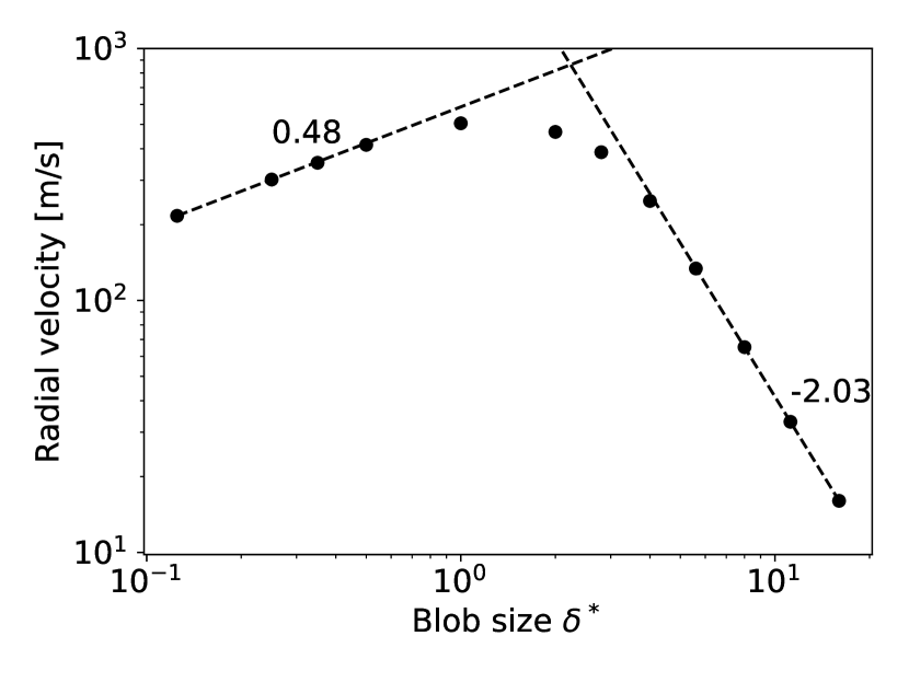
(a) Radial velocity $v_{r}$ of an isothermal plasma blob as a function of blob size $\delta$. Analytical scalings are $v_{r}\sim\sqrt{\delta}$ for $\delta/\delta^{*}\ll 1$, and $v_{r}\sim\left(\delta/\delta^{*}\right)^{-2}$ for $\delta/\delta^{*}\gg 1$.

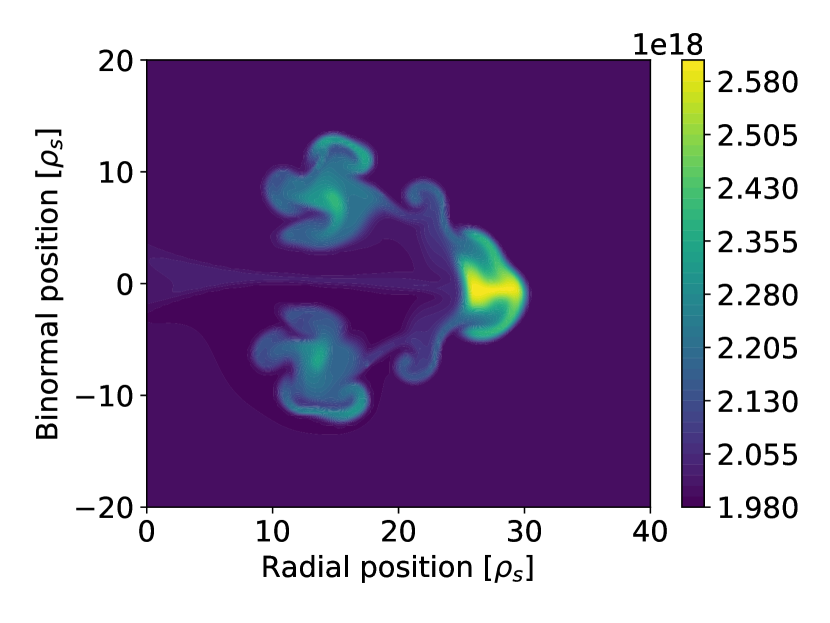
(b) Electron density $n_{e}$ at $t=1500/\omega_{ci}=44.7\mu$s for a $\delta^{*}$-sized seeded blob.

Figure 11: Solution to equations 3 in a 2D domain perpendicular to the magnetic field, starting with a circular cross section density perturbation and driven by magnetic field curvature. Input and analysis scripts in Hermes-3 repository examples/blob2d.

This model extends quite straightforwardly to include hot ion effects and separate ion and electron temperatures, by modifying the input file to introduce a new species h+ with a separate pressure equation. The vorticity formulation is implemented such that the polarisation current contribution of multiple species is included in calculating the electric field; The self-consistent calculation of the polarisation drift on the ion species density in a multi-ion species calculation has recently been implemented and is being tested. Further examples, tests and applications may be found in the Hermes-3 manual [44] and source code repository [40].

5 Conclusions

Advancing understanding of the physics of the edge of tokamak plasmas drives the need for increasingly complex models. To address this need a new open-source plasma simulation tool has been developed that enables researchers to perform complex multi-species plasma simulations by combining reusable software components. This is achieved by building on the BOUT++ framework of partial differential equation solvers, and defining a flexible yet robust method of coupling components together within a parallelised high-performance code.

Applications of this tool to simulations of tokamak plasmas have been demonstrated: Time dependent simulations of plasma filament/blob propagation and steady-state transport including atomic reactions. Convergence tests and comparisons to analytic solutions have been carried out, demonstrating good conservation properties and convergence of the methods. The public Git repository includes a suite of unit, integrated and Method of Manufactured Solutions (MMS) tests that are used routinely to check the correctness of code changes.

Areas for future development and research have been identified: Extending the steady state solver implemented using PETSc from 1D transport problems (section 4.1) to 2D is a high priority, as is benchmarking of Hermes-3 against other codes for both transport and turbulence applications. These efforts have begun and will be reported elsewhere once completed.

Hermes-3 is publicly available [40] on Github under a GPL-3 license. To maximise its utility to the plasma community a set of examples are included, and a manual [44] provides an introduction for new users.

Appendix A Numerical method for parallel dynamics

Dynamics parallel to the magnetic field are solved using a 2^nd-order slope-limiter method, briefly described in section 2.2. For any number of fluids we solve the number density $n$, momentum along the magnetic field, $mnv_{||}$, and either pressure $p$ or energy $\mathcal{E}$. Here $m$ is the particle mass, so that $mn$ is the mass density. $v_{||}$ is the component of the flow velocity in the direction of the magnetic field, and is aligned with one of the mesh coordinate directions. All quantities are cell centered.

Cell edge values are by default reconstructed using a MinMod method (other limiters are available, including 1st-order upwind, Monotonized Central, and Superbee). If $f_{i}$ is the value of field $f$ at the center of cell $i$, then using MinMod slope limiter the gradient $g$ inside the cell is:

$$g_{i}=\left\{\begin{array}[]{ll}0&\textrm{if $\left(f_{i+1}-f_{i}\right)\left(f_{i}-f_{i-1}\right)<0$}\\ f_{i+1}-f_{i}&\textrm{if $\left|f_{i+1}-f_{i}\right|<\left|f_{i}-f_{i-1}\right|$}\\ f_{i}-f_{i-1}&\textrm{Otherwise}\end{array}\right.$$ (4)

The values at the left and right of cell $i$ are:

$$f_{i,R} =f_{i}+g_{i}/2$$

$$f_{i,L} =f_{i}-g_{i}/2$$ (5)

This same reconstruction is performed for $n$, $v_{||}$ and $p$ (or $\mathcal{E}$). The flux $\Gamma_{i+1/2}$ between cell $i$ and $i+1$ is:

$$\Gamma_{f,i+1/2}=\frac{1}{2}\left(f_{i,R}v_{||i,R}+f_{i+1,L}v_{||i+1,L}\right)+\frac{a_{max,i+1/2}}{2}\left(f_{i,R}-f_{i+1,L}\right)$$ (6)

This includes a Lax flux term that penalises jumps across cell edges, and depends on the maximum local wave speed, $a_{max}$. Momentum is not reconstructed at cell edges; Instead the momentum flux is calculated from the cell edge densities and velocities:

$$\Gamma_{nv,i+1/2}=\frac{1}{2}\left(n_{i,R}v_{||i,R}^{2}+n_{i+1,L}v_{||i+1,L}^{2}\right)+\frac{a_{max,i+1/2}}{2}\left(n_{i,R}v_{||i,R}-n_{i+1,L}v_{||i+1,R}\right)$$ (7)

The wave speeds, and so $a_{max}$, depend on the model being solved, so can be customised to e.g include or exclude Alfvén waves or electron thermal speed. For simple neutral fluid simulations it is:

$$a_{max,i+1/2}=\max\left(\left|v_{||i}\right|,\left|v_{||i+1}\right|,\sqrt{\frac{\gamma p_{i}}{mn_{i}}},\sqrt{\frac{\gamma p_{i+1}}{mn_{i+1}}}\right)$$ (8)

The divergence of the flux, and so the rate of change of $f$ in cell $i$, depends on the cell area perpendicular to the flow, $A_{i}$, and cell volume $V_{i}$:

$$\nabla\cdot\left(\mathbf{b}fv_{||}\right)_{i}=\frac{1}{V_{i}}\left[\frac{A_{i}+A_{i+1}}{2}\Gamma_{f,i+1/2}-\frac{A_{i-1}+A_{i}}{2}\Gamma_{f,i-1/2}\right]$$ (9)

A.1 Boundaries

At boundaries along the magnetic field the flow of particles and energy are set by e.g. Bohm sheath boundary conditions or no-flow conditions. To ensure that the flux of particles is consistent with the boundary condition imposed at cell boundaries, fluxes of density $n$ and also $p$ or $\mathcal{E}$ are set to the simple mid-point flux:

$$\Gamma_{f,i+1/2}^{boundary}=f_{i+1/2}v_{||i+1/2}$$ (10)

where $f_{i+1/2}=\frac{1}{2}\left(f_{i}+f_{i+1}\right)$ and $v_{||i+1/2}=\frac{1}{2}\left(v_{||i}+v_{||i+1}\right)$ are the mid-point averages where boundary conditions are imposed. It has been found necessary to include dissipation in the momentum flux at the boundary, to suppress numerical overshoots due to the narrow boundary layers that can form:

$$\Gamma_{nv,i+1/2}^{boundary}=n_{i,R}v_{||i,R}v_{||i+1/2}+a_{max}\left[n_{i,R}v_{||i,R}-n_{i+1/2}v_{||i+1/2}\right]$$ (11)

where $n_{i+1/2}=\frac{1}{2}\left(n_{i}+n_{i+1}\right)$.

Appendix B Plasma and neutral atom transport equations

The equations solved in 1D in section 4.1 and in 2D in section 4.2 are detailed here for completeness. A total of seven spatially varying quantities are evolved in time: The deuterium ion and atom densities ($n_{d+}$ and $n_{d}$); the flow of ions and atoms parallel to the magnetic field ($v_{||,d+}$ and $v_{||,d}$); and the pressure of the ions, atoms, and electrons ($p_{d+}$, $p_{d}$ and $p_{e}$). SI units are used except temperatures, which are in eV. In a 1D domain (section 4.1) the anomalous diffusion terms are omitted and all derivatives perpendicular to the magnetic field are assumed to be zero.

The equations for the deuterium ion species density $n_{d+}$, parallel velocity $v_{||,d+}\equiv\mathbf{b}\cdot\mathbf{v}_{d+}$ and pressure $p_{d+}=en_{d+}T_{d+}$ are:

$$\frac{\partial}{\partial t}n_{d+}= -\nabla\cdot\left[\left(\mathbf{b}v_{||,d+}+\mathbf{v}_{\perp,d+}\right)n_{d+}\right]+R_{iz}-R_{rc}$$ (12a)

$$\frac{\partial}{\partial t}\left(m_{d+}n_{d+}v_{||,d+}\right)= -\nabla\cdot\left[\left(\mathbf{b}v_{||,d+}+\mathbf{v}_{\perp,d+}\right)m_{d+}n_{d+}v_{||,d+}\right]-\mathbf{b}\cdot\nabla p_{d+}$$

$$+en_{d+}E_{||}+R_{cx}m_{d}\left(v_{||,d}-v_{||,d+}\right)$$

$$-R_{rc}m_{d}v_{||,d+}+R_{iz}m_{d}v_{||,d}$$ (12b)

$$\frac{\partial}{\partial t}\left(\frac{3}{2}p_{d+}\right)= -\nabla\cdot\left[\left(\mathbf{b}v_{||,d+}+\mathbf{v}_{\perp,d+}\right)\frac{5}{2}p_{d+}\right]+v_{||,d+}\mathbf{b}\cdot\nabla p_{d+}$$

$$+\nabla\left(\mathbf{b}\kappa_{||,d+}\mathbf{b}\cdot\nabla T_{d+}\right)+\nabla\cdot\left(\chi_{d+}n_{d+}\nabla_{\perp}T_{d+}\right)$$

$$+\frac{1}{2}m_{d}\left(R_{cx}+R_{iz}\right)\left(v_{||,d}-v_{||,d+}\right)^{2}$$

$$+R_{iz}\frac{3}{2}eT_{d}-R_{rc}\frac{3}{2}eT_{d+}+W_{d+,e}$$ (12c)

where $\mathbf{b}=\mathbf{B}/B$ is the unit vector in the direction of the magnetic field, and the gradient in the plane perpendicular to the magnetic field is $\nabla_{\perp}\equiv\nabla-\mathbf{b}\mathbf{b}\cdot\nabla$. Particle diffusion across the magnetic field is implemented as a cross-field ion drift velocity $\mathbf{v}_{\perp,d+}$ with diffusion coefficient $D$:

$$\mathbf{v}_{\perp,d+}=-D\frac{1}{n_{d+}}\nabla_{\perp}n_{d+}$$ (13)

The charge exchange (CX), ionization (IZ) and recombination (RC) reactions between species have rates (events per m³ per second):

$$R_{cx}= n_{d+}n_{d}\left<\sigma v\right>_{cx}$$ (14a)

$$R_{iz}= n_{e}n_{d}\left<\sigma v\right>_{iz}$$ (14b)

$$R_{rc}= n_{e}n_{d+}\left<\sigma v\right>_{rc}$$ (14c)

where the Maxwellian-averaged cross sections $\left<\sigma v\right>$ are taken from Amjuel [63], specifically Amjuel reaction H.4 2.1.5 (ionisation), H.4 2.1.8 (recombination) and H.3 3.1.8 (charge exchange). Hydrogenic charge-exchange reactions are adjusted for isotope mass, ion and neutral temperatures by calculating an effective temperature $T_{eff}=T_{atom}/A_{atom}+T_{ion}/A_{ion}$ as described in the Amjuel manual.

There is a transfer of thermal energy to ions from electrons due to collisions, $W_{d+,e}$:

$$W_{d+,e}=3\nu_{d+,e}n_{d+}\frac{m_{d+}}{m_{d+}+m_{e}}e\left(T_{e}-T_{d+}\right)$$ (15)

with ion-electron collision frequency $\nu_{d+,e}=\nu_{e,d+}m_{e}/m_{d+}$.

The electron density $n_{e}=n_{d+}$ is set by quasineutrality; the electron parallel velocity $v_{||,e}=v_{||,d+}$ from assuming that the parallel current is zero (Note that this is a choice in this particular model, not a general feature of Hermes-3). The electron pressure equation is:

$$\frac{\partial}{\partial t}\left(\frac{3}{2}p_{e}\right)= -\nabla\cdot\left[\left(\mathbf{b}v_{||,e}+\mathbf{v}_{\perp,d+}\right)\frac{5}{2}p_{e}\right]+v_{||,e}\mathbf{b}\cdot\nabla p_{e}$$

$$+\nabla\left(\mathbf{b}\kappa_{||,e}\mathbf{b}\cdot\nabla T_{e}\right)+\nabla\cdot\left(\chi_{e}en_{e}\nabla_{\perp}T_{e}\right)$$

$$-E_{iz}+E_{rc}-W_{d+,e}$$ (16a)

where $E_{iz}$ and $E_{rc}$ are the energy cost and gain due to ionization and recombination atomic processes respectively. These are calculated using Amjuel [63], reactions 2.1.5 and 2.1.8. Ionization always removes energy from the electrons; Recombination may be either a source or sink of electron energy, depending on the temperature and density. Electron force balance is used to calculate the parallel electric field $E_{||}\equiv\mathbf{b}\cdot\mathbf{E}$ and so transfer electron pressure $p_{e}$ forces to the ions:

$$en_{e}E_{||}=-\mathbf{b}\cdot\nabla p_{e}-\nabla\cdot\left[\mathbf{v}_{\perp,d+}m_{e}n_{e}v_{||,e}\right]$$ (17)

The equations for the neutral deuterium atom density $n_{d}$, parallel velocity $v_{||,d}$ and pressure $p_{d}=en_{d}T_{d}$ are:

$$\frac{\partial}{\partial t}n_{d}= -\nabla\cdot\left[\left(\mathbf{b}v_{||,d}+\mathbf{v}_{\perp,d}\right)n_{d}\right]-R_{iz}+R_{rc}$$ (18a)

$$\frac{\partial}{\partial t}\left(m_{d}n_{d}v_{||,d}\right)= -\nabla\cdot\left[\left(\mathbf{b}v_{||,d}+\mathbf{v}_{\perp,d}\right)m_{d}n_{d}v_{||,d}\right]-\mathbf{b}\cdot\nabla p_{d}$$

$$-R_{cx}m_{d}\left(v_{||,d}-v_{||,d+}\right)+R_{rc}m_{d}v_{||,d+}$$

$$-R_{iz}m_{d}v_{||,d}$$ (18b)

$$\frac{\partial}{\partial t}\left(\frac{3}{2}p_{d}\right)= -\nabla\cdot\left[\left(\mathbf{b}v_{||,d}+\mathbf{v}_{\perp,d}\right)\frac{5}{2}p_{d}\right]+v_{||,d}\mathbf{b}\cdot\nabla p_{d}$$

$$+\nabla\left(\kappa_{d}\nabla T_{d}\right)+\frac{1}{2}m_{d}\left(R_{cx}+R_{rc}\right)\left(v_{||,d}-v_{||,d+}\right)^{2}$$

$$-R_{iz}\frac{3}{2}eT_{d}+R_{rc}\frac{3}{2}eT_{d+}$$ (18c)

The flow of neutral atoms across the magnetic field, $\mathbf{v}_{\perp,d}$, is derived by balancing friction forces against pressure gradient [2]:

$$\mathbf{v}_{\perp,d}=-\frac{T_{d}}{m_{d}\nu_{d}p_{d}}\nabla_{\perp}p_{d}$$ (19)

The thermal conduction coefficients for each species are:

$$\kappa_{||,d+}=3.9\frac{p_{d+}}{m_{d+}\nu_{d+}}\qquad\kappa_{||,e}=3.16\frac{p_{e}}{m_{e}\nu_{e}}\qquad\kappa_{d}=\frac{p_{d}}{m_{d}\nu_{d}}$$ (20)

The collision frequencies for each species, $\nu_{d+}$, $\nu_{e}$ and $\nu_{d}$, are:

$$\nu_{d+}= \nu_{d+,d+}+\frac{m_{e}}{m_{d+}}\nu_{e,d+}+n_{d}\left<\sigma v\right>_{cx}$$ (21a)

$$\nu_{e}= \nu_{e,d+}+\nu_{e,e}$$ (21b)

$$\nu_{d}= n_{d+}\left<\sigma v\right>_{cx}+n_{d}a_{0}\sqrt{2eT_{d}/m_{d}}$$ (21c)

The collision frequency of charged species $a$ on charged species $b$ is given by [75]:

$$\nu_{a,b}=\frac{q_{a}q_{b}n_{b}\log\Lambda\left(1+m_{a}/m_{b}\right)}{3\pi^{3/2}\epsilon_{0}^{2}m_{a}^{2}\left(v_{a}^{2}+v_{b}^{2}\right)^{3/2}}$$ (22)

with $v_{a}^{2}=2T_{a}/m_{a}$. Neutral-neutral collisions assume a kinetic diameter of $2.8\times 10^{-10}$m (cross-section $a_{0}=2.5\times 10^{-19}$m²), chosen based on typical values for species considered ($2.89\times 10^{-10}$m for H₂, $2.60\times 10^{-10}$m for He, $2.75\times 10^{-10}$m for Ne [76]).

The Coulomb logarithm is different for electron-electron, ion-ion and electron-ion species interactions, and is calculated using the NRL formulary [77] (page 34). Converted to SI units with $T$ in eV the Coulomb logarithms are:

$$\log\Lambda_{e,e}= 30.4-0.5\log n_{e}+\frac{5}{4}\log T_{e}-\sqrt{\epsilon+\left(\log T_{e}-2\right)^{2}/16}$$ (23a)

$$\log\Lambda_{e,i}= \left\{\begin{array}[]{c c}31-0.5\log n_{e}+\log T_{e}&\textrm{if }T_{i}\frac{m_{e}}{m_{i}}<10Z_{i}^{2}<T_{e}\\ 30-0.5\log n_{e}-\log Z_{i}+1.5\log T_{e}&\textrm{if }T_{i}\frac{m_{e}}{m_{i}}<T_{e}<10Z_{i}^{2}\\ 23-0.5\log n_{i}+1.5\log T_{i}-\log\left(Z_{i}^{2}A_{i}\right)&\textrm{if }T_{e}<T_{i}m_{e}/m_{i}\end{array}\right.$$ (23e)

$$\log\Lambda_{i,i}= 29.91-\log\left[\frac{Z_{1}Z_{2}\left(A_{1}+A_{2}\right)}{A_{1}T_{2}+A_{2}T_{1}}\sqrt{n_{1}Z_{1}^{2}/T_{1}+n_{2}Z_{2}^{2}/T_{2}}\right]$$ (23f)

Note that earlier versions of the NRL formulary had a factor of $A_{i}^{-1}$ rather than $A_{i}$ in equation 23e.

References

- [1] B.D.Dudson et al. CPC 180, 1467-1480 (2009)

References

- [1] R. Schneider, X. Bonnin, K. Borrass, D. P. Coster, H. Kastelewicz, D. Rieter, V. A. Rozhansky, B. J. Braams, Contrib. Plasma Phys. 46 (1-2) (2006) 3–191. doi:10.1002/ctpp.200610001.
- [2] T. D. Rognlien, X. Q. Xu, A. C. Hindmarsh, J. Comput. Phys. 175 (2002) 249–268.
-
[3]
R. Simonini, G. Corrigan, G. Radford, J. Spence, A. Taroni,
Models and Numerics in the
Multi-Fluid 2-D Edge Plasma Code EDGE2D/U, Contrib. Plasma Phys. 34 (1994)
368–373.
doi:10.1002/ctpp.2150340242.
URL https://doi.org/10.1002/ctpp.2150340242 -
[4]
Z. H. Wang, X. Q. Xu, T. Y. Xia, T. D. Rognlien,
2D simulations of
transport dynamics during tokamak fuelling by supersonic molecular beam
injection 54 (4) (2014) 043019.
doi:10.1088/0029-5515/54/4/043019.
URL https://doi.org/10.1088/0029-5515/54/4/043019 -
[5]
M. Giacomin, P. Ricci, A. Coroado, G. Fourestey, D. Galassi, E. Lanti,
D. Manchini, N. Richart, L. N. Stenger, N. Varini,
The GBS code for the self-consistent
simulation of plasma turbulence and kinetic neutral dynamics in the tokamak
boundary, arXiv (2021) 2112.03573.
URL https://arxiv.org/abs/2112.03573 - [6] F. D. Halpern, P. Ricci, S. Jolliet, J. Loizu, J. Morales, A. Mosetto, F. Musil, F. Riva, T. M. Tran, C. Wersal, The GBS code for tokamak scrape-off layer simulations, Journal of Computational Physics 315 (2016) 388–408. doi:10.1016/j.jcp.2016.03.040.
- [7] P. Ricci, F. D. Halpern, S. Jolliet, J. Loizu, A. Mosetto, A. Fasoli, I. Furno, C. Theiler, Plasma Phys. Control. Fusion 54 (2012) 124047.
- [8] P. Tamain, P. Ghendrih, E. Tsitrone, V. Grandgirard, X. Garbet, Y. Sarazin, E. Serre, G. Ciraolo, G. Chiavassa, J. Comput. Phys. 229 (2) (2010) 361–378. doi:10.1016/j.jcp.2009.09.031.
- [9] P. Tamain, H. Bufferand, G. Ciraolo, C. Colin, D. Galassi, P. Ghendrih, F. Schwander, E. Serre, J. Comput. Phys. 321 (2016) 606–623. doi:10.1016/j.jcp.2016.05.038.
- [10] J. Madsen, V. Naulin, A. H. Nielsen, J. J. Rasmussen, Collisional transport across the magnetic field in drift-fluid models, Physics of Plasmas 23 (3) (2016) 032306. doi:10.1063/1.4943199.
-
[11]
B. D. Dudson, et al., Comp. Phys. Comm. 180 (2009) 1467–1480.
doi:DOI:10.1016/j.cpc.2009.03.008,
[link].
URL http://www.sciencedirect.com/science/article/B6TJ5-4VTCM95-3/2/ed200cd23916d02f86fda4ce6887d798 -
[12]
B. D. Dudson, et al. 81 (01) (2015) 365810104.
doi:10.1017/S0022377814000816,
[link].
URL http://doi.org/10.1017/S0022377814000816 - [13] BOUT++ contributors, BOUT++ manual, https://bout-dev.readthedocs.io/.
-
[14]
B. D. Dudson, J. Leddy, Plasma Phys. Control. Fusion 59 (2017) 054010.
doi:10.1088/1361-6587/aa63d2,
[link].
URL https://doi.org/10.1088/1361-6587/aa63d2 -
[15]
L. Easy, F. Militello, J. Omotani, B. Dudson, E. Havlíčková, P. Tamain,
V. Naulin, A. H. Nielsen, Three
dimensional simulations of plasma filaments in the scrape off layer: A
comparison with models of reduced dimensionality, Physics of Plasmas 21 (12)
(2014) 122515.
arXiv:https://doi.org/10.1063/1.4904207, doi:10.1063/1.4904207.
URL https://doi.org/10.1063/1.4904207 - [16] L. Easy, F. Militello, T. Nicholas, J. Omotani, F. Riva, N. Walkden, UKAEA, Storm drift-reduced plasma fluid model, https://github.com/boutproject/STORM.
-
[17]
H. Bufferand, P. Tamain, S. Baschetti, J. Bucalossi, G. Ciraolo, N. Fedorczak,
P. Ghendrih, F. Nespoli, F. Schwander, E. Serre, Y. Marandet,
Three-dimensional
modelling of edge multi-component plasma taking into account realistic wall
geometry, Nuclear Materials and Energy 18 (2019) 82–86.
doi:https://doi.org/10.1016/j.nme.2018.11.025.
URL https://www.sciencedirect.com/science/article/pii/S2352179118302035 -
[18]
A. Coroado, P. Ricci, A
self-consistent multi-component model of plasma turbulence and kinetic
neutral dynamics for the simulation of the tokamak boundary, arXiv (2021)
2110.13335.
URL https://arxiv.org/abs/2110.13335 -
[19]
S. Raj, N. Bisai, V. Shankar, A. Sen, J. Ghosh, R. L. Tanna, M. B. Chowdhuri,
K. A. Jadeja, K. Asudani, T. Macwan, S. Aich, K. Singh,
Studies on
impurity seeding and transport in edge and SOL of tokamak plasma, Nuclear
Fusion (2021).
doi:10.1088/1741-4326/ac44b0.
URL http://iopscience.iop.org/article/10.1088/1741-4326/ac44b0 -
[20]
J. Leddy, B. Dudson, H. Willett,