MV-MR: multi-views and multi-representations for self-supervised learning and knowledge distillation

Abstract

We present a new method of self-supervised learning and knowledge distillation based on the multi-views and multi-representations (MV-MR). The MV-MR is based on the maximization of dependence between learnable embeddings from augmented and non-augmented views, jointly with the maximization of dependence between learnable embeddings from augmented view and multiple non-learnable representations from non-augmented view. We show that the proposed method can be used for efficient self-supervised classification and model-agnostic knowledge distillation. Unlike other self-supervised techniques, our approach does not use any contrastive learning, clustering, or stop gradients. MV-MR is a generic framework allowing the incorporation of constraints on the learnable embeddings via the usage of image multi-representations as regularizers. Along this line, knowledge distillation is considered a particular case of such a regularization. MV-MR provides the state-of-the-art performance on the STL10 and ImageNet-1K datasets among non-contrastive and clustering-free methods. We show that a lower complexity ResNet50 model pretrained using proposed knowledge distillation based on the CLIP ViT model achieves state-of-the-art performance on STL10 linear evaluation. The code is available at: github.com/vkinakh/mv-mr

1 Introduction

Self-supervised learning (SSL) methods are alternatives to supervised ones. In recent years, the gap between SSL and supervised methods decreased in the downstream tasks that include image classification [1], object detection [2] and semantic image segmentation [3], [4]. A general idea behind the SSL models for image classification is to train an embedding network, often called an encoder, on the unlabeled dataset and then to use this pretrained encoder for the downstream tasks either by training a classifier on top of the frozen embeddings or by fine-tuning the whole model. The general goal is to ensure the invariance of embeddings to different inputs known as augmentations or views. However, this approach might lead to trivial solutions when two branches of encoders produce the same output. This might result in a collapse in training. Therefore, there have been a lot of recent works tackling this issue by regularizing the networks to avoid such a collapse. To prevent these negative effects, there exist several major approaches that use different tricks: (a) direct mutual information maximization between the input image $\bf x$ and the embedding $\bf z$ like in InfoNCE [5] and associated contrastive loss with positive-negative pairs that are very costly in practice, (b) methods that avoid the collapse by introducing different asymmetries into two branches at the training stage, like training one network with gradient descent and updating the other one with an exponential moving average of the weights from the first one [6] or introducing regularizers on the learned representations such as decorrelation regularization on the dimensions of the embeddings [7] etc.

The proposed approach avoids the collapse by introducing the dependence maximization between trainable embeddings and hand-crafted features using distance correlation[8]. Distance correlation, unlike other losses in latent space, allows computing dependencies between feature vectors of different shapes. We maximize the dependence between different embeddings while preserving the variance in them. We show that variance preservation maximizes the entropy of embeddings that makes them unique and distinguishable. Our approach is different from InfoNCE[5], which advocates a contrastive loss, that maximizes the mutual information (MI) between input image $\bf x$ and its embeddings $\bf z$. In contrast to the InfoNCE, our approach is not contrastive, does not require large batch sizes, and has multiple advantages in practice while dealing with large images. It is also different from methods such as Barlow Twins [7] and VICReg [9] since we do not explicitly minimize the dependencies between the components within the embedding.

We also show that the proposed approach can be used for efficient model and latent space-agnostic knowledge distillation. The approach is based on the dependence maximization between the embeddings of the target trainable encoder, represented by the ResNet50[10], and the embeddings of the pretrained encoder, represented by the CLIP[11] based on ViT-B-16[12]. Since the distance correlation is agnostic to the latent space shape, any pretrained encoder with any latent space can be used for knowledge distillation. To our best knowledge, we propose the first method that allows for knowledge distillation for models with the latent space of different shapes without any labels.

The main goal behind MV-MR is twofold: (i) maximizing the invariance of embeddings, i.e., maximizing the proximity of embeddings for the same image observed under different views, and (ii) maximizing the amount of information in each embedding, i.e., maximizing the variability of the embedding. Furthermore, to avoid the collapse at training, we regularize the branch with the augmentations by imposing the dependence constraints on a set of representations extracted from various encodings.

The novelty behind the proposed approach can be summarized as follows: (i) we introduce a novel SSL approach that avoids collapse thanks to an additional regularization term that maximizes the dependence between trainable embeddings and feature vectors using distance correlation; (ii) up to our best knowledge, the proposed method is among the first that uses the dependence maximization of the latent space based on distance correlation for SSL; (iii) the proposed method is agnostic to the latent space shape, thus can be used with any type of features; (iv) we introduce a novel knowledge distillation technique, that is agnostic to model and shape of latent space; (v) we demonstrate the state-of-the-art classification results on STL10 (89.71%) and ImageNet-1K (74.5%) datasets using linear evaluation protocol for noncontrastive SSL methods; (vi) we provide the information-theoretic explanation of the proposed method that contributes to the explainable ML; (vii) we demonstrate how the complex CLIP model with 86.2M of parameters trained on 400M text-image pairs can be distilled to a ResNet50 model with just 23.5M parameters trained on 1.3M images of ImageNet-1K.

We have three terms in our objective function: (a) the first term $\mathcal{L}_{1}$ consists of the mean square error (MSE) loss between the embeddings from non-augmented view and augmented views of the same image, which is used for the invariance of embeddings, and additional variation terms that are used for maximization of the variability of the embeddings; (b) the second term $\mathcal{L}_{2}$ stands for the distance correlation between the embeddings from the augmented and non-augmented views that complements the first term to capture non-linear relations between the embeddings that go beyond the second order statistics and (c) the third term $\mathcal{L}_{3}$ corresponds to the distance correlation between the embeddings from augmented view and multiple non-learnable image representations. As the non-learnable or hand-crafted representations, we have studied various techniques of invariant data representation that are well-known in computer vision and image processing applications. The studied hand-crafted features include but are not limited by: ScatNet [13] features, local standard deviation (LSD) based [14] filters, and histograms of oriented gradients (HOG) [15]. Besides, to demonstrate the flexibility of the proposed method, we have also considered random augmentations of the original images flattened into feature vectors as instances of hand-crafted features.

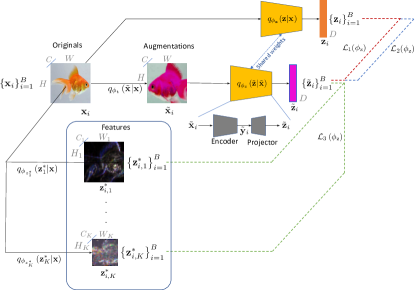
Figure 1: MV-MR: proposed SSL approach. Two views of the image are produced: one original and the other augmented by $q_{\phi_{\mathrm{t}}}(\tilde{\mathbf{x}}|\mathbf{x})$, then these views are encoded via encoder $q_{\phi_{\mathbf{z}}}(\mathbf{z}|\mathbf{x})$, producing ${\bf z}_{i}$ that denotes an original embedding and $\tilde{\mathbf{z}}_{i}$ denoting an augmented one. The representations $\mathbf{z}_{i,k}^{*}$ are obtained via via $K$ hand-crafted feature extraction mappers $q_{\phi_{z_{k}^{*}}}\left(\mathbf{z}_{k}^{*}|\mathbf{x}\right),1\leq k\leq K$. The same process is applied to each image ${\bf x}_{i}$ in the batch $1\leq i\leq B$. The embedding is regularized by a loss $\mathcal{L}_{1}(\phi_{\mathrm{z}})$ minimizing the Euclidean distances between the embeddings ${\bf z}_{i}$ and $\tilde{\mathbf{z}}_{i}$ while ensuring that their variance is above a threshold. The loss $\mathcal{L}_{2}(\phi_{\mathrm{z}})$ ensures the dependence between the pair of augmented and non-augmented embeddings using the distance correlation. The regularization loss $\mathcal{L}_{3}(\phi_{\mathrm{z}})$ is imposed by maximizing the distance correlation between the augmented embedding $\tilde{\mathbf{z}}_{i}$ and a set of hand-crafted features $\mathbf{z}_{i,k}^{*},1\leq k\leq K$ computed for the given batch $B$.

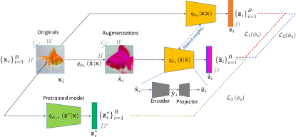
Figure 2: MV-MR: distillation approach. $q_{\phi_{z^{*}}}(\textbf{z}^{*}|\textbf{x})$ is the complex teacher model used as a feature extractor in order to train a light student model $q_{\phi_{z}}\left(\mathbf{z}|\mathbf{x}\right)$.

2 MV-MR: motivation and intuition

MV-MR pretraining and distillation schemes are schematically shown in Figures 1, 2. The dimensions of embeddings with and without augmentations are the same, i.e., $\tilde{\bf{z}}\in\mathbb{R}^{D}$ and ${\bf z}\in\mathbb{R}^{D}$. These embeddings are extracted from the augmented $\tilde{\bf x}$ and non-augmented $\bf{x}$ via a generalized embedder $q_{\phi_{z}}(\cdot|\cdot)$ that can be deterministic or stochastic. A $k^{th}$ hand-crafted descriptor ${\bf{z}}_{k}^{*}$, with $k\in\{1,2,\cdots,K\}$ and $K$ stands for the total number of hand-crafted descriptors, is generally a tensor of dimensions $H_{k}\times W_{k}\times C_{k}$ and is flattened to $D_{k}=H_{k}W_{k}C_{k}$. This description is generally obtained via deterministic assignment ${\mathbf{z}_{k}^{*}}=f_{\phi_{z_{k}^{*}}}({\bf x})$ or sometimes stochastic mapping ${\bf Z}^{*}_{k}\sim q_{\phi_{z_{k}^{*}}}\left(\mathbf{z}_{k}^{*}|\mathbf{x}\right)$.

2.1 Motivation: regularisation in self-supervised representation learning

The learned representation should contain the informative representation of data with lower dimensionality and should be invariant under some transformations, i.e., to ensure the same latent representation for the data from the same sample passed through certain transformations. The satisfaction of these conflicting requirements in practice is not a trivial task. Many state-of-the-art SSL techniques try to find a reasonable compromise between these requirements and practical feasibility solely in the scope of machine learning formulation by imposing certain constraints on the properties of the learned representation via the optimization of encoder parameters under augmentations.

At the same time, there exists a rich body of achievements in the computer vision community in the domain of the hand-crafted design of robust, invariant yet discriminating data representations[16][17][18][15]. Generally, the computer vision descriptors are very rich in terms of targeted invariant features and quite efficient in terms of computation. However, to our best knowledge, such descriptors are not yet fully integrated into the development of SSL techniques. Therefore, one of the objectives of this paper is to propose a framework where the SSL representation learning might be coupled with the constraints on the embedding space offered by the invariant computer vision representations. Our objective is not to consider a case-by-case approach on how to couple SSL with a particular computer vision representation but instead to propose a generic approach where any form of desirable computer vision representation can be integrated into the SSL optimization problem in an easy and tractable way. This ensures that the learned representation possesses the targeted properties inherited from the used computer vision descriptors. Furthermore, features extracted by such descriptors might be considered as a form of invariant data representations which is one of the desired properties of trained encoders. Thus, maximizing the dependence between the trainable embedding and such representation might be a novel form of regularization leading to the increased invariance yet collapse-avoiding technique. Since a single computer vision descriptor might not capture all desirable properties and have different representation formats, the targeted framework should be flexible enough to deal uniformly with all these descriptors within a simple optimization problem.

In summary, our motivation is to include regularization constraints on the solution by borrowing some inherent computer vision feature invariance to certain transformations. In this way, we will target learning the low dimensional embedding which contains only essential information about the data that might be of interest for the targeted downstream task and where all information about the augmentations is excluded.

2.2 Intuition

The basic idea behind MV-MR is to introduce constraints on the invariance of embedding via a new loss function. Our overall objective is to maximize the mutual information $I(\tilde{\bf Z};{\bf Z})$ between the augmented embedding $\tilde{\bf Z}$ and the embedding without the augmentation $\bf Z$ and mutual information $I(\tilde{\bf Z};{\bf Z}_{k}^{*})$ between $\tilde{\bf Z}$ and some invariant feature ${\bf Z}_{k}^{*}$ extracted from $\bf X$ using a mapper ensuring a known invariance to the desired transformation.

2.2.1 Measuring dependencies between embeddings of non-augmented and augmented data

Upper bound on mutual information: In the first case, one can decompose the mutual information as:

$$I(\tilde{\bf Z};{\bf Z}) =\mathbb{E}_{p(\tilde{\bf z},{\bf z})}\left[{\log\frac{p({\tilde{\bf z}},{\bf z})}{p(\tilde{\bf z})p({\bf z})}}\right] =\mathbb{E}_{p(\tilde{\bf z},{\bf z})}\left[{\log\frac{p({\tilde{\bf z}}|{\bf z})}{p(\tilde{\bf z})}}\right]$$ (1)

$$=h(\tilde{\bf Z})-h(\tilde{\bf Z}|{\bf Z}).$$

The maximization of this mutual information is equivalent to the maximization of the differential entropy $h(\tilde{\bf Z})=-\mathbb{E}_{p(\tilde{\bf z})}\left[\log{p(\tilde{\bf z})}\right]$ and the minimization of conditional differential entropy $h(\tilde{\bf Z}|{\bf Z})=-\mathbb{E}_{p(\tilde{\bf z},{\bf z})}\left[{\log p({\tilde{\bf z}}|{\bf z})}\right]$ . Since the computation of the marginal distribution $p(\tilde{\bf z})$ and conditional distribution $p({\tilde{\bf z}}|{\bf z})$ is difficult in practice, we will proceed with bounding these terms. We assume that the desired embeddings need to be bounded by some variance $\sigma_{z}^{2}$ to avoid a training collapse when the encoders produce constant and non-informative vectors so that the entropy maximizing distribution for the first entropy term is the Gaussian one, i.e., $p(\tilde{\bf z})\propto 1/C_{0}\text{exp}(-\beta_{z}{\bf C}_{\tilde{\mathrm{z}}\tilde{\mathrm{z}}})$, where $C_{0}$ stands for the normalization constant, $\beta_{z}$ denotes scaling and ${\bf C}_{\tilde{\mathrm{z}}\tilde{\mathrm{z}}}=\sigma_{z}^{2}{\bf I}_{D}$, where ${\bf I}_{D}$ denotes the identity matrix of dimension $D\times D$. The conditional entropy $h(\tilde{\bf Z}|{\bf Z})$ is minimized when the embedding $\tilde{\bf Z}$ contains as much as possible information about ${\bf Z}$, i.e., when two vectors are dependent. Assuming that $p(\tilde{{\bf z}}|{\bf z})\propto 1/C_{1}\text{exp}(-\beta_{zz}d(\tilde{{\bf z}},{\bf z}))$, where $d(\tilde{{\bf z}},{\bf z})$ denotes some distance between two vectors such as $\ell_{2}$-norm for the Gaussian distribution or $\ell_{1}$-norm for Laplacian one, the minimization of the conditional entropy $h(\tilde{\bf Z}|{\bf Z})$ reduces to the minimization of the distance $d(\tilde{{\bf z}},{\bf z})$.

Distance covariance: Another way to measure the dependency between the data is based on distance covariance proposed by [8]. In the general case of dependence between the data, the distance covariance is non-invariant to strictly monotonic transformations, unlike mutual information. Nevertheless, the distance covariance has several attractive properties: (i) it can be efficiently computed for two vectors that have generally different dimensions $\tilde{\bf z}\in\mathbb{R}^{D}$ and ${\bf z}\in\mathbb{R}^{D^{\prime}}$ and (ii) it is easier to compute in practice in contrast to the mutual information. Additionally, the distance covariance captures higher-order dependencies between the data in contrast to the Pearson correlation. The distance covariance $\operatorname{dCov}^{2}(\tilde{\mathbf{Z}},\mathbf{Z})$ measures the distance between the joint characteristic function $\varphi_{\mathbf{Z},\tilde{\mathbf{Z}}}(\mathbf{t},\mathbf{u})$ and the product of the marginal characteristic functions $\varphi_{\mathbf{Z}}(\mathbf{t})\varphi_{\tilde{\mathbf{Z}}}(\mathbf{u})$[8]. This definition has a lot of similarities to the mutual information (1) which measures the ratio between the joint distribution $p({\tilde{\bf z}},{\bf z})$ and the product of marginals $p(\tilde{\bf z})p({\bf z})$. Since $\varphi_{\mathbf{Z},\tilde{\mathbf{Z}}}(\mathbf{t},\mathbf{u})=\varphi_{\mathbf{Z}}(\mathbf{t})\varphi_{\tilde{\mathbf{Z}}}(\mathbf{u})$ when $\tilde{\mathbf{Z}}$ and $\mathbf{Z}$ are independent random vectors, then the distance covariance is equal to zero.

In the following, we will proceed with the normalized version of distance covariance known as distance correlation defined as:

$$\operatorname{dCor}(\tilde{\textbf{Z}},\textbf{Z})=\frac{\mathrm{dCov}^{2}(\tilde{\textbf{Z}},\textbf{Z})}{\sqrt{\mathrm{dVar}(\tilde{\textbf{Z}})\mathrm{dVar}(\textbf{Z})}},$$ (2)

where $\textbf{Z}=[\textbf{z}_{1},...,\textbf{z}_{B}]$ denotes a batch of size $B$ of embeddings from original views, $\tilde{\textbf{Z}}=[\tilde{\textbf{z}}_{1},...,\tilde{\textbf{z}}_{B}]$ stands for a batch of embeddings from augmented views and:

$$\mathrm{dCov}_{B}^{2}(\tilde{\textbf{Z}},\textbf{Z}):=\frac{1}{B^{2}}\sum_{j=1}^{B}\sum_{i=1}^{B}A_{j,i}C_{j,i}.$$ (3)

Note that $\mathrm{dVar}(\textbf{Z})=\mathrm{dCov}_{B}^{2}({\textbf{Z}},\textbf{Z})$. In equation (3), we use the notations $A_{j,i}:=a_{j,i}-\bar{a}_{j\cdot}-\bar{a}_{\cdot i}+\bar{a}_{\cdot\cdot},\quad$ $C_{j,i}:=c_{j,i}-\bar{c}_{j\cdot}-\bar{c}_{\cdot i}+\bar{c}_{\cdot\cdot}$, where $\quad a_{j,i}=\left\|\tilde{\textbf{Z}}_{j}-\tilde{\textbf{Z}}_{i}\right\|,\quad$ $c_{j,i}=\left\|\textbf{Z}_{j}-\textbf{Z}_{i}\right\|$, where $j,i=1,2,\ldots,B$.

2.2.2 Dependence between embeddings of augmented data and multiple hand-crafted representations

The second mutual information $I(\tilde{\bf Z};{\bf Z}_{k}^{*})$ between $\tilde{\bf Z}$ and some invariant feature ${\bf Z}_{k}^{*}$ deals with the vectors of different dimensions. Thus, one can either map these vectors to the same dimension and apply the above arguments, use Hilbert-Schmidt proxy [19], or proceed with the distance correlation dependence measure for the uniformity of consideration. We focus on the distance correlation case due to its property of handling vectors of different dimensions and its ability to capture higher-order data statistics.

3 Related work

Pretext task methods. The main idea behind these methods is to design a specific task a.k.a. pretext task for the dataset which will contain some "labels" of the pretext task without having any access to the labels of the target task. Such pretext tasks include but are not limited to: applying and predicting parameters of the geometric transformations [20], jigsaw puzzle solving [21], etc., inpainting [22]and colorization [23] of the images and reversing augmentations. Typically, the pretext task methods and coupled with other SSL techniques in recent years [24], [25], [26].

Contrastive methods. Most of the contrastive SSL methods are based on different extensions of the InfoNCE[5] formulation. The InfoNCE method is based on the direct maximization of the mutual information between the input image $\bf{X}$ and its embedding $\bf{Z}$, via minimization of the contrastive loss. Thus, the estimation of the distributions $p(\bf{z}|\bf{x})$ and $p(\bf{z})$ with the marginalization over $\tilde{\bf{X}}$. The examples of contrastive methods are SimCLR[27], SwAV [28], DINO [29].

Clustering methods. Clustering-based SSL methods are based on the idea of assigning cluster labels to the learned representations in an unsupervised manner with some regularization like maintaining uniformity of these cluster labels. DeepCluster [30] method iteratively groups the features from the encoder using the standard k-means clustering and then uses them as an assignment for the supervision to update the weights of the encoder at the next iterations. SwAV [28] and DINO[29] are other notable clustering-based SSL methods that combine contrastive learning and clustering by clustering the data while requiring the same cluster assignment for different views of the same image.

Distillation methods. Distillation-based SSL methods like BYOL [31], SimSiam [6] and others use the teacher-student type of training, where the student network is trained with the gradient descent, while the teacher network is not updated with gradient descent, but rather with an exponential moving average update or other methods. Such a design is used to avoid collapse.

Collapse preventing methods. Similar to distillation, collapse-preventing methods try to prevent the collapse by the usage of special regularization of embeddings. Barlow Twins [7] method aims at making the covariance matrix of the embeddings to be an identity matrix. It means that each dimension of the embeddings should be decorrelated with all other dimensions. Additionally, the minimum variance of embedding per each dimension in the batch is constrained. VICReg [9] method extends the Barlow Twins [7] approach by imposing an additional constraint on the distance between the embeddings with and without augmentations.

Knowledge distillation. Knowledge distillation[32] is a type of model optimization, where a simple small model (student model) is trained to match the bigger complex model (teacher model). There are multiple types of knowledge distillation schemes: offline distillation[33], online distillation[34], and self-distillation[35]. There are multiple types of knowledge types, used for distillation: response-based knowledge[33],[36] feature-based knowledge[37], and others. We show how our method can be used as offline feature-based knowledge distillation.

4 MV-MR: detailed description

4.1 Method

The training objective consists of two parts (a) ensuring the invariance of the learned representation under the applied augmentations and simultaneously (b) imposing constraints on the learned representation. The final loss integrates the loss based on the upper bound of the mutual information and distance correlation.

4.1.1 Training objectives for the representation learning based on the mutual information

We follow the overall idea of ensuring the invariance of learned representation under the family of applied augmentations and we proceed along the line discussed in the previous section. Since both branches have the same dimension $D$, we proceed with the maximization of the upper bound on the mutual information between these dimensions as considered in section 2.2.1.

To train the encoder, we penalize the embeddings of augmented view $\tilde{\mathbf{z}}_{i}$ to be as close as possible to the embeddings of non-augmented view $\mathbf{z}_{i}$ using MSE loss 4 between them:

$$d\left(\mathbf{Z},\tilde{\mathbf{Z}}\right)=\frac{1}{B}\sum_{i=1}^{B}\left\|\mathbf{z}_{i}-\tilde{\mathbf{z}}_{i}\right\|_{2}^{2}.$$ (4)

Even though MSE is one of the most common losses for ensuring closeness between the embeddings, we show that this term corresponds to the conditional entropy term in the mutual information 1.

The variance regularization term corresponding to the entropy term in the mutual information 1 is used to control the variance of the embeddings. We use a hinge function of the standard deviation of the embeddings along the batch dimension:

$$v(\mathbf{Z})=\frac{1}{D}\sum_{d=1}^{D}\max\left(0,\gamma-S\left(\textbf{z}[d],\epsilon\right)\right),$$ (5)

where $\mathbf{z}[d]$ denotes the $d^{th}$ dimension of $\bf z$, $S$ is the standard deviation defined as:

$$S(a,\epsilon)=\sqrt{\operatorname{Var}(a)+\epsilon},$$ (6)

and $\gamma$ is the margin parameter for the standard deviation, $\epsilon$ is a small scalar for numerical stability.

The corresponding loss that ensures the correspondence between the embeddings from the augmented and non-augmented views and the variance of both embeddings is defined as:

$$\mathcal{L}_{1}(\phi_{z})=\lambda d\left(\textbf{Z},\tilde{\textbf{Z}}\right)+\mu\left[v(\textbf{Z})+v\left(\tilde{\textbf{Z}}\right)\right],$$ (7)

where $\lambda$ and $\mu$ are hyper-parameters controlling the importance of each term in the loss. This loss is parametrized by the parameters $\phi_{z}$ of the encoder and projector. It should be pointed out that for the symmetry, we impose the constraint on the variance for both augmented and non-augmented embeddings.

It is interesting to point out that the obtained result coincides with the loss used in VICReg[9] where its origin was not considered from the information-theoretic point of view as the maximization of mutual information between the embeddings. At the same time, it should be noted that there is no constraint on the covariance matrix of embeddings as in VICReg[9] and Barlow Twins [7] methods.

4.1.2 Training objectives for representation learning based on distance covariance

The distance correlation is used for the dependence maximization between the embedding from the augmented view with the non-augmented one and the set of representations from the hand-crafted functions.

Accordingly, the loss $\mathcal{L}_{2}(\phi_{z})$ denotes the minimization formulation of the distance correlation maximization problem between embeddings from augmented and non-augmented views:

$$\mathcal{L}_{2}(\phi_{z})=\alpha\left[1-\mathrm{dCor}(\tilde{\textbf{Z}},{\textbf{Z}})\right],$$ (8)

and the loss $\mathcal{L}_{3}(\phi_{z})$ denotes the same for the embedding from the augmented view and $k^{th}$ hand-crafted representation:

$$\mathcal{L}_{3}(\phi_{z})=\sum_{k=1}^{K}{\beta_{k}\left[1-\mathrm{dCor}(\tilde{\textbf{Z}},\textbf{Z}_{k}^{*})\right]},$$ (9)

where $\alpha$ and $\beta_{k}$ are hyper-parameters controlling the importance of each term in the loss. In our experiments, we set $\alpha=1$ and perform a grid search on the values of $\lambda$ and $\mu$ with the base condition $\lambda=\mu>1$ and $\beta_{k}=1$.

The final loss function is a sum of three losses:

$$\mathcal{L}\left(\phi_{z}\right)=\mathcal{L}_{1}(\phi_{z})+\mathcal{L}_{2}(\phi_{z})+\mathcal{L}_{3}(\phi_{z}).$$ (10)

5 Applications of proposed model

In this section, we demonstrate the application of the proposed model to a) self-supervised pretraining of the model and b) self-supervised model distillation.

5.1 Self-supervised pretraining for classification

The proposed method can be used for efficient self-supervised model pretraining for the classification. Once pretrained, the model is finetuned for classification. We report our results on STL10 and ImageNet-1K datasets on linear evaluation and semi-supervised finetuning with 1% and 10% of labels pipelines in Table 1, and Table 2. In a linear evaluation pipeline, the pretrained encoder is used as it, without further training, while only a one-layer linear classifier is trained with labeled data. In the semi-supervised finetuning pipeline, the classifier head is attached to the pretrained encoder and the full model is finetuned on the labeled data.

5.2 Knowledge distillation

The proposed method can also be used for efficient knowledge distillation. It is done by using the pretrained model (teacher) as the feature extractor and computing the distance correlation between the embeddings of the trainable encoder (student) and the pretrained teacher encoder. In practice, this can be used to match the performance of the big pretrained models with smaller models or match the performance of the models that have been trained on proprietary datasets. In contrast to the standard knowledge distillation approaches [33], our approach does not use any labels, nor require the latent space of the same shape. As a practical example, we demonstrate that by using the proposed knowledge distillation approach, we are able to match the performance of the CLIP[11] based on ViT-B-16[12] with 86.2M parameters pretrained on 400M images from LAION-400M[38] dataset, by the ResNet50 with 23.5M parameters pretrained on STL10 and ImageNet-1K datasets as shown in section 6.2. Then the distilled model can be used for downstream tasks such as classification.

6 Results

In this section, we will demonstrate the performance of the proposed method for two downstream tasks: (a) SSL-based classification and (b) knowledge distillation-based classification.

6.1 SSL based classification

We evaluate the representations obtained after the pretraining ResNet50 backbone with MV-MR on ImageNet-1K [39] and STL-10 [40] datasets for 1000 epochs using the loss function described above. The model pretrained on ImageNet-1K is evaluated with linear protocol and semi-supervised protocol with 1% and 10% of labeled images.

6.1.1 Evaluation on ImageNet-1K

Linear evaluation protocol: A linear classifier is trained on top of the frozen representations of the ResNet50 pretrained using MV-MR for 100 epochs with the cross-entropy loss. Semi-supervised evaluation protocol: The pretrained ResNet50 is fine-tuned with a fraction of the ImageNet-1K dataset: 1% or 10% of sampled labels for 100 epochs with the cross-entropy loss.

The results on the validation set of ImageNet-1K for linear and semi-supervised evaluation protocols of the model pretrained on the training set of ImageNet-1K are shown in Table 1. The main advantage of the MV-MR is that it presents a new way of regularizing latent space for self-supervised pretraining by using distance correlation between the embeddings from the model and hand-crafted image features. Due to the lack of computational resources, we did not run the parameters optimization for ImageNet-1K pretraining, so we think that the results might be further improved.

Method Linear Semi-supervised Top 1 Top 5 Top 1 Top 5 1% 10% 1% 10% Supervised 76.5 - 25.4 56.4 48.4 80.4 PIRL [41] 63.6 - - - - - SimSiam [6] 71.3 - - - - - InfoMin Aug [42] 73.0 91.1 - - - - OBoW [43] 73.8 - - - - - BYOL [31] 74.3 91.6 53.2 68.8 78.4 89.0 Barlow Twins [7] 73.2 91.0 55.0 69.7 79.2 89.3 VICReg [9] 73.2 91.1 54.8 69.5 79.4 89.5 MV-MR (ours) 74.5 92.1 56.1 69.9 79.4 89.5

Table 1: Evaluation on ImageNet-1K. Evaluation of the representations from ResNet50 non-contrastive backbones pretrained with MV-MR on: (1) linear evaluation protocol on top of frozen representations from ImageNet; (2) semi-supervised classification on top of fine-tuned representations with 1% and 10% of labeled ImageNet samples.

6.1.2 Evaluation STL10

In this study, we wanted to demonstrate the method performance when directly training on a small-size dataset. Each class is represented by about 500 images per class. The results on the test set of STL10 [40] dataset for linear evaluation protocol of the model pretrained on the training and unlabeled subsets of STL10 are shown in Table 2.

The model was trained with the following hand-crafted features: flattened original and augmented images, ScatNet features, HOG features, and LSD features. Our model achieves state-of-the-art results in the linear evaluation protocol on the STL10 dataset. In the linear evaluation protocol, the linear model is trained on the training subset of STL10. The model is not evaluated on a semi-supervised evaluation protocol. The proposed model demonstrates the best performance among the compared methods.

Method	STL10
ADC [44]	53.0
IIC [45]	61
TSUK [46]	66.5
SCAN [47]	80.9
ScatSimCLR [24]	85.1
RUC [48]	86.7
MV-MR (ours)	89.7

Table 2: Evaluation on STL10. Classification accuracy for the linear evaluation protocol on top of frozen representations from STL10 dataset.

6.1.3 Transfer learning

To evaluate the pretrained representation of multiclass classification on the VOC07[49] dataset, we train a linear classifier on top of the frozen representations from the pretrained encoder for 100 epochs. The mAP on the VOC07 dataset is reported in Table 3 along with the results from other non-contrastive state-of-the-art SSL methods with a ResNet50 as a backbone.

Method	Linear Classification
	VOC07
Supervised	87.5
PIRL [41]	81.1
BYOL [31]	86.6
OBoW [43]	89.3
Barlow Twins [7]	86.2
VICReg [9]	86.6
MV-MR(ours)	87.1

Table 3: Transfer learning on multiclass classification on VOC07[49] dataset. Evaluation of the non-contrastive representations from pretrained model on multiclass classification using the linear classifier on top of frozen representations. We report mAP.

6.2 Knowledge distillation based classification

To evaluate the proposed approach to the knowledge distillation-based classification, we have used pretrained CLIP[11] model based on ViT-B-16[12] encoder as the teacher and the ResNet50[10] as the student model. The CLIP is trained based on the contrastive loss between the image and text embeddings. To proceed with the knowledge distillation in the same way as for the SSL training, we use the default projector $8192-8192-8192$ after the ResNet50 encoder. The pretrained CLIP ViT model uses images of the shape $224\times 224$ as an input and outputs the latent vector of the shape 512, as shown in Figure 2. The teacher model is evaluated using zero-shot evaluation and linear evaluation pipelines. The student model is evaluated only using a linear evaluation pipeline.

The goal of the experimental validation is to demonstrate whether the ResNet50 model with 23.5M parameters trained only on 1.3M images can provide similar performance to the CLIP based on the ViT model with 86.2M parameters, trained on 400M images. It is important to point out that the training is performed without any additional labels according to the proposed knowledge distillation framework. In Table 4, we report results of knowledge distillation, where CLIP based on ViT-B-16 is used as a teacher model and ResNet50 as a student model. The model is only trained for 200 epochs using the proposed knowledge distillation approach on ImageNet-1K and then evaluated on STL10 and ImageNet-1K datasets. The obtained results confirm that the convolutional ResNet50 model with 4$\times$ fewer parameters in comparison to the transformer ViT teacher model and trained on a considerably smaller amount of unlabeled data can closely approach the performance of the teacher model without any special labeling, clustering, additional augmentations, or complex contrastive losses. It is also important to point out that the CLIP model trained on 400M text-image pairs initially outperformed all previous SSL methods for the STL-10 dataset. Remarkably, the proposed knowledge distillation largely preserved this performance and achieved 95.6% versus the best SSL MV-MR result 89.7% as indicated in Tables 2, 4. Thus, both the proposed MV-MR SSL training and knowledge distillation achieve state-of-the-art results on the STL-10 dataset and competitive results for the ImageNet-1K among all non-contrastive and clustering-free SSL methods.

Approach Parameters STL10 ImageNet-1K CLIP ViT-B-16 (zero-shot) 86.2M 96.8 67.1 CLIP ViT-B-16 (linear evaluation) 86.2M 98.5 77.4 MV-MR ResNet50 (linear evaluation) 23.5M 95.6 75.3

Table 4: Knowledge distillation experiment with ImageNet-1K as training dataset, CLIP based on ViT-B-16 as teacher model, and ResNet50 as a student model.

6.3 Ablation studies

In this subsection, we describe the ablation studies on losses (Tables 5). In each of the experiments, we use the same training and evaluation setup: dataset: STL10, epochs: $100$, batch size: $64$, 16-bit precision, batch accumulation: $1$ batch. We use a linear evaluation pipeline. We demonstrate the impact of representation learning based on the maximization of the considered upper bound on the mutual information and the maximization of distance covariance in various settings. In this ablation, we show that the best results are achieved when using three loss terms: $\mathcal{L}_{1}$, $\mathcal{L}_{2}$, and $\mathcal{L}_{2}$. The ablation studies on augmentations and feature extractors are presented in the supplementary material.

			Accuracy
$\mathcal{L}_{1}$	$\mathcal{L}_{2}$	$\mathcal{L}_{3}$	Top 1	Top 5
1 loss
✓			50.86	93.95
	✓		46.71	92.18
		✓	44.1	92.08
2 losses
✓	✓		50.76	93.83
✓		✓	47.39	92.54
	✓	✓	40.06	89.31
3 losses
✓	✓	✓	69.38	98.85

Table 5: Ablation studies on the combination of losses. We check the importance of each loss term for the training of the model. It is shown that using loss terms $\mathcal{L}_{1}$, $\mathcal{L}_{2}$ and $\mathcal{L}_{3}$ provides the best classification performance. Also, we observe a phenomenon in which loss terms $\mathcal{L}_{2}$ and $\mathcal{L}_{3}$ work the best when applied jointly with the loss $\mathcal{L}_{1}$. However, it is interesting to point out that a disjoint usage of these losses does not lead to reasonable performance enhancement. The exact nature of this phenomenon is not completely clear and additional investigation should be performed.

More ablation studies: a study on the hand-crafted features used, a study on the augmentation used during training, and a study on the shape of the projector are presented in the supplementary material.

7 Implementation details

The architecture of the MV-MR is similar to ones used in other SSL methods such BarlowTwins [7], VICReg [9], and others. The model $f_{\phi_{z}}$, shown in Figure 1, consists of two main parts: (i) the encoder, which is used for downstream tasks, and (ii) the projector, which is used for the mapping of encoder outputs to the embeddings used for training loss functions 1. In our experiments, we use standard ResNet50 [10] available in $torchvision$ library[50] as the encoder and projector, which consists of two linear layers of the size $8192$ followed by batch normalization and ReLU and output linear layer.

In our experiments, we use computer vision feature extraction methods applied to the original data: original RGB image, that is being flattened into a feature vector, ScatNet features of the image[51], random augmented images, flatten into a feature vector, histogram of oriented gradients (HOG), and local standard deviation filter (LSD filter)[14].

ScatNet transform: ScatNet [13, 51] is a class of Convolutional Neural Networks (CNNs) that has a set of useful properties: (i) deformation stability, (ii) fixed weights, (iii) sparse representations, (iv) interpretable representation.

Random augmented image: In our experiments, we have applied the following augmentations to the image: random cropping, horizontal flipping, random color augmentations, grayscale and Gaussian blur. Then the image is flattened into a 1-dimensional feature vector.

HOG: Histogram of oriented gradients (HOG) [15] is a feature description that is based on the counting of occurrences of gradient orientation in the localized portion of an image.

LSD filter: A local standard deviation filter[14] is a filter that computes a standard deviation in a defined image region over the image. The region is usually of a rectangular shape of size $3\times 3$ or $5\times 5$ pixels.

We use the PyTorch framework [50] for the implementation of the proposed approach. We use ScatNet with the following parameters: $J=2$ and $L=8$. We use the HOG feature extractor with the following parameters: number of bins $24$ and pool size $8$. We use a kernel of the size 3x3 in the STD filter. As augmentations for both image representation and as the input to the encoder we use: random resized cropping, random horizontal flipping with probability $0.5$, random color jittering augmentation with brightness $0.8$, contrast $0.8$, saturation $0.8$, hue $0.2$ and probability $0.8$, random grayscale with probability $0.2$ and Gaussian blur of the kernel size $0.1$ of the image size, mean $0$ and sigma in range the $[0.1,2]$.

For the losses, the margin parameter $\gamma$ is set to $1$ and $\epsilon$ is set to $1e-4$ in $v(\mathbf{Z})=\frac{1}{D}\sum_{d=1}^{D}\max\left(0,\gamma-S\left(\textbf{z}[d],\epsilon\right)\right)$.

During self-supervised pretraining experiments, that are presented in Table 1 and Table 2, we train models for $1000$ epochs, batch size $256$, gradient accumulation every 4 steps, base learning rate $1e-4$, Adam[52] optimizer, cosine learning rate schedule and $16$-bit precision. During linear evaluation on STL10 and ImageNet-1K, we train a single-layer linear model for $100$ epochs with a batch size $256$, learning rate $1e-4$, and Adam optimizer. During semi-supervised evaluation on ImageNet-1K, we train a model for $100$ epochs with a batch size $128$, learning rate $1e-4$, and Adam optimizer. During the knowledge distillation, we train the model for $200$ epochs, with $512$ batch size, base learning rate $1e-4$, Adam[52] optimizer, cosine learning rate schedule, and $16$-bit precision.

When training, weight parameters $\lambda=1$ and $\mu=1$ in in $\mathcal{L}_{1}$, $\alpha=1$ in $\mathcal{L}_{2}$ and $\beta_{k}=1,k=1...K$ in $\mathcal{L}_{3}$.

8 Conclusions

In this paper, we introduce novel self-supervised MV-MR learning and knowledge distillation approaches, which are based on the maximization of the several dependency measures between two embeddings obtained from views with and without augmentations and multiple representations extracted from non-augmented views. The proposed methods use an upper bound on mutual information and a distance correlation for the dependence estimation for the representations of different dimensions. We explain the intuition behind the proposed method of upper bound on the mutual information and the usage of distance correlation as a dependence measure. Our method achieves state-of-the-art self-supervised classification on the STL10 dataset and achieves comparable state-of-the-art results on ImageNet-1K datasets on linear evaluation and semi-supervised evaluations. We show that ResNet50 pretrained using knowledge distillation on CLIP ViT-B-16 achieves comparable performance with far fewer parameters.

Appendix A Distance correlation definition

The distance correlation[8] term between the batch of embeddings of augmented view $\tilde{\textbf{Z}}$ and the batch of embeddings of original view Z is computed by utilizing the following formula:

$$\mathrm{d}\operatorname{Cor}(\tilde{\textbf{Z}},\textbf{Z})=\frac{\mathrm{dCov}^{2}(\tilde{\textbf{Z}},\textbf{Z})}{\sqrt{\mathrm{dVar}(\tilde{\textbf{Z}})\mathrm{dVar}(\textbf{Z})}},$$ (11)

where $\textbf{Z}=[\textbf{z}_{1},...,\textbf{z}_{B}]$ - batch of embeddings from original views, $\tilde{\textbf{Z}}=[\tilde{\textbf{z}}_{1},...,\tilde{\textbf{z}}_{B}]$ - batch of embeddings from augmented views and:

$$\mathrm{dCov}_{B}^{2}(\tilde{\textbf{Z}},\textbf{Z}):=\frac{1}{B^{2}}\sum_{j=1}^{B}\sum_{i=1}^{B}A_{j,i}C_{j,i}.$$ (12)

The distance correlation term between the batch of embeddings of augmented views $\tilde{\mathbf{Z}}$ and the batch of features computed from the original views $\mathbf{Z}^{*}$ is computed by the following formula:

$$\mathrm{dCor}(\tilde{\textbf{Z}},\textbf{Z}^{*})=\frac{\mathrm{dCov}^{2}(\tilde{\textbf{Z}},\textbf{Z}^{*})}{\sqrt{\mathrm{dVar}(\tilde{\textbf{Z}})\mathrm{dVar}(\textbf{Z}^{*})}},$$ (13)

where $\textbf{Z}^{*}=[\textbf{z}^{*}_{1},...,\textbf{z}^{*}_{B}]$ - batch of features computed from original views and

$$\mathrm{dCov}_{B}^{2}(\tilde{\textbf{Z}},\textbf{Z}^{*}):=\frac{1}{B^{2}}\sum_{j=1}^{B}\sum_{i=1}^{B}A_{j,i}D_{j,i}.$$ (14)

In formulas 12, 14 $A_{j,i}:=a_{j,i}-\bar{a}_{j\cdot}-\bar{a}_{\cdot i}+\bar{a}_{\cdot\cdot},\quad$ $C_{j,i}:=c_{j,i}-\bar{c}_{j\cdot}-\bar{c}_{\cdot i}+\bar{c}_{\cdot\cdot},\quad$ $D_{j,i}:=d_{j,i}-\bar{d}_{j\cdot}-\bar{d}_{\cdot i}+\bar{d}_{\cdot\cdot}$ where $\quad a_{j,i}=\left\|\tilde{\textbf{Z}}_{j}-\tilde{\textbf{Z}}_{i}\right\|,\quad$ $c_{j,i}=\left\|\textbf{Z}_{j}-\textbf{Z}_{i}\right\|\quad$ and $d_{j,i}=\left\|\textbf{Z}^{*}_{j}-\textbf{Z}^{*}_{i}\right\|,\quad$ where $j,i=1,2,\ldots,B$.

Appendix B Ablation studies

Original image ScatNet Augmented image HOG LSD Accuracy Top 1 Top 5 1 feature ✓ 58.82 96.81 ✓ 54.12 95.23 ✓ 63.51 97.81 ✓ 54.15 95.26 ✓ 53.94 95.44 2 features ✓ ✓ 64.44 97.97 ✓ ✓ 66.18 98.39 ✓ ✓ 63 97.78 ✓ ✓ 63.14 97.8 ✓ ✓ 63.3 97.78 ✓ ✓ 62.95 97.6 ✓ ✓ 59.41 96.78 ✓ ✓ 63.66 97.69 ✓ ✓ 60.21 96.8 ✓ ✓ 62.46 97.71 3 features ✓ ✓ ✓ 65.82 98.18 ✓ ✓ ✓ 65.52 97.97 ✓ ✓ ✓ 60.96 97.08 ✓ ✓ ✓ 65.11 98.12 ✓ ✓ ✓ 65.19 98 ✓ ✓ ✓ 65.37 98.29 ✓ ✓ ✓ 65.45 98.18 ✓ ✓ ✓ 64.35 97.93 ✓ ✓ ✓ 60.63 97.1 ✓ ✓ ✓ 64.9 98.08 4 features ✓ ✓ ✓ ✓ 68.25 98.45 ✓ ✓ ✓ ✓ 68.2 98.53 ✓ ✓ ✓ ✓ 64.56 97.44 ✓ ✓ ✓ ✓ 67.21 98.48 ✓ ✓ ✓ ✓ 67.05 98.22 5 features ✓ ✓ ✓ ✓ ✓ 69.38 98.85

Table 6: Ablation studies of the combinations of features used for the $\mathcal{L}_{3}$ loss. In this setup, all three losses are used: $\mathcal{L}_{1}$ and $\mathcal{L}_{2}$ and $\mathcal{L}_{3}$. ScatNet transformation of the original image. Augmented image - randomly augmented original image. HOG - histogram of oriented gradients computed from original view. LSD - original view filtered with the local standard deviation filter. Since all of these features are images, they are flattened before computing distance correlation.

In this section, we describe the ablation studies on the combination of features for loss term $\mathcal{L}_{3}$ (Table 6), a number of layers, and size of the projector in the trainable encoder (Table 8), and image augmentations (Table 7). In each of the experiments, we use the same training and evaluation setup: dataset: STL10[40], epochs: $100$, batch size: $64$, 16-bit precision, batch accumulation: $1$ batch. When pretraining, all 3 loss terms are used. After model pretraining, it is evaluated using linear evaluation.

We describe the ablation studies on the combinations of features used for the $\mathcal{L}_{3}$ loss term in combination with loss terms $\mathcal{L}_{1}$ and $\mathcal{L}_{2}$ in Tables 6. We study the impact of features on the classification accuracy of the model. We use the following features in the study: the original image flattened into a vector, ScatNet[51] features of the original image, an augmented image flattened into a vector, and a histogram of oriented gradients of the original image, and features from the local standard deviation filter (LSD). We use ScatNet with the following parameters: $J=2$ and $L=8$. We use the HOG[15] feature extractor with the following parameters: number of bins $24$ and pool size $8$. Kernel of the size 3x3 is used in the LSD filter[14]. As augmentations for image representation we use: random resized cropping, random horizontal flipping with probability $0.5$, random color jittering augmentation with brightness $0.8$, contrast $0.8$, saturation $0.8$, hue $0.2$ and probability $0.8$, random grayscale with probability $0.2$ and Gaussian blur of the kernel size $0.1$ of the image size, mean $0$ and sigma in range the $[0.1,2]$. We show that the best results are achieved, when we use the combination of all feature extractors, mentioned above.

Random Crop Horizontal Flip Color Grayscale Blur Accuracy Top 1 Top 5 ✓ 43.02 90.31 ✓ ✓ 49.99 93.98 ✓ ✓ ✓ 50.58 93.76 ✓ ✓ ✓ ✓ 70.82 98.96 ✓ ✓ ✓ ✓ ✓ 69.38 98.85

Table 7: Ablation studies on the image augmentations.

The ablation studies on image augmentations are presented in Table 7. As augmentations, we compare random resized cropping, random horizontal flipping, random color augmentations, random grayscale, and random Gaussian blur. We use the same parameters for each augmentation, as when augmented images are used as features. We show that the best classification results are achieved when a combination of random cropping, horizontal flipping, color jittering, and random grayscale is used.

Projector size	Accuracy
8192-8192-8192	69.38
4096-4096-4096	51.90
2048-2048-2048	51.35
1024-1024-1021	51.86
512-512-512	49.40
256-256-256	49.02
8192-8192	49.90
4096-4096	48.81
2048-2048	48.66
1024-1024	48.73
512-512	48.06
256-256	48.07
8192	48.65
4096	48.51
2048	48.20
1024	47.61
512	46.11
256	47.17
without projector	16.70

Table 8: Ablation studies on the projector. Projectors consist of blocks with linear layers, batch normalization, and ReLU activation. We always keep the last layer linear.

The ablation studies on the number of layers and their size in the encoder’s projects are presented in Table 8. When the number of layers is bigger than one in the projector, it consists of blocks with linear layers, batch normalization, and ReLU activation. We always keep the last layer linear. We show the best classification results are shown when the projector consists of 3 layers, each with $8192-8192-8192$ neurons.

References

- Zhou et al. [2021] Jinghao Zhou, Chen Wei, Huiyu Wang, Wei Shen, Cihang Xie, Alan Yuille, and Tao Kong. ibot: Image bert pre-training with online tokenizer. arXiv preprint arXiv:2111.07832, 2021.
- Huang et al. [2022] Gabriel Huang, Issam Laradji, David Vazquez, Simon Lacoste-Julien, and Pau Rodriguez. A survey of self-supervised and few-shot object detection. IEEE Transactions on Pattern Analysis and Machine Intelligence, 2022.
- Zheng et al. [2021] Hao Zheng, Jun Han, Hongxiao Wang, Lin Yang, Zhuo Zhao, Chaoli Wang, and Danny Z Chen. Hierarchical self-supervised learning for medical image segmentation based on multi-domain data aggregation. In International Conference on Medical Image Computing and Computer-Assisted Intervention, pages 622–632. Springer, 2021.
- Punn and Agarwal [2022] Narinder Singh Punn and Sonali Agarwal. Bt-unet: A self-supervised learning framework for biomedical image segmentation using barlow twins with u-net models. Machine Learning, pages 1–16, 2022.
- Oord et al. [2018] Aaron van den Oord, Yazhe Li, and Oriol Vinyals. Representation learning with contrastive predictive coding. arXiv preprint arXiv:1807.03748, 2018.
- Chen and He [2021] Xinlei Chen and Kaiming He. Exploring simple siamese representation learning. In Proceedings of the IEEE/CVF Conference on Computer Vision and Pattern Recognition, pages 15750–15758, 2021.
- Zbontar et al. [2021] Jure Zbontar, Li Jing, Ishan Misra, Yann LeCun, and Stéphane Deny. Barlow twins: Self-supervised learning via redundancy reduction. In International Conference on Machine Learning, pages 12310–12320. PMLR, 2021.
- Székely et al. [2007] Gábor J Székely, Maria L Rizzo, and Nail K Bakirov. Measuring and testing dependence by correlation of distances. The annals of statistics, 35(6):2769–2794, 2007.
- Bardes et al. [2021] Adrien Bardes, Jean Ponce, and Yann LeCun. Vicreg: Variance-invariance-covariance regularization for self-supervised learning. arXiv preprint arXiv:2105.04906, 2021.
- He et al. [2016] Kaiming He, Xiangyu Zhang, Shaoqing Ren, and Jian Sun. Deep residual learning for image recognition. In Proceedings of the IEEE conference on computer vision and pattern recognition, pages 770–778, 2016.
- Radford et al. [2021] Alec Radford, Jong Wook Kim, Chris Hallacy, Aditya Ramesh, Gabriel Goh, Sandhini Agarwal, Girish Sastry, Amanda Askell, Pamela Mishkin, Jack Clark, et al. Learning transferable visual models from natural language supervision. In International Conference on Machine Learning, pages 8748–8763. PMLR, 2021.
- Dosovitskiy et al. [2021] Alexey Dosovitskiy, Lucas Beyer, Alexander Kolesnikov, Dirk Weissenborn, Xiaohua Zhai, Thomas Unterthiner, Mostafa Dehghani, Matthias Minderer, Georg Heigold, Sylvain Gelly, Jakob Uszkoreit, and Neil Houlsby. An image is worth 16x16 words: Transformers for image recognition at scale. ICLR, 2021.
- Oyallon et al. [2018] Edouard Oyallon, Sergey Zagoruyko, Gabriel Huang, Nikos Komodakis, Simon Lacoste-Julien, Matthew Blaschko, and Eugene Belilovsky. Scattering networks for hybrid representation learning. IEEE transactions on pattern analysis and machine intelligence, 41(9):2208–2221, 2018.
- Narendra and Fitch [1981] Patrenahalli M Narendra and Robert C Fitch. Real-time adaptive contrast enhancement. IEEE transactions on pattern analysis and machine intelligence, (6):655–661, 1981.
- Dalal and Triggs [2005] Navneet Dalal and Bill Triggs. Histograms of oriented gradients for human detection. In 2005 IEEE computer society conference on computer vision and pattern recognition (CVPR’05), volume 1, pages 886–893. Ieee, 2005.
- LOEW [2004] David G LOEW. Distinctive image features from scale-invariant keypoints. International journal of computer vision, 2004.
- Rublee et al. [2011] Ethan Rublee, Vincent Rabaud, Kurt Konolige, and Gary Bradski. Orb: An efficient alternative to sift or surf. In 2011 International conference on computer vision, pages 2564–2571. Ieee, 2011.
- Pietikäinen and Zhao [2015] Matti Pietikäinen and Guoying Zhao. Two decades of local binary patterns: A survey. In Advances in independent component analysis and learning machines, pages 175–210. Elsevier, 2015.
- Gretton et al. [2007] Arthur Gretton, Kenji Fukumizu, Choon Teo, Le Song, Bernhard Schölkopf, and Alex Smola. A kernel statistical test of independence. In J. Platt, D. Koller, Y. Singer, and S. Roweis, editors, Advances in Neural Information Processing Systems, volume 20. Curran Associates, Inc., 2007. URL https://proceedings.neurips.cc/paper/2007/file/d5cfead94f5350c12c322b5b664544c1-Paper.pdf.
- Gidaris et al. [2018] Spyros Gidaris, Praveer Singh, and Nikos Komodakis. Unsupervised representation learning by predicting image rotations. arXiv preprint arXiv:1803.07728, 2018.
- Noroozi and Favaro [2016] Mehdi Noroozi and Paolo Favaro. Unsupervised learning of visual representations by solving jigsaw puzzles. In European conference on computer vision, pages 69–84. Springer, 2016.
- Pathak et al. [2016] Deepak Pathak, Philipp Krahenbuhl, Jeff Donahue, Trevor Darrell, and Alexei A Efros. Context encoders: Feature learning by inpainting. In Proceedings of the IEEE conference on computer vision and pattern recognition, pages 2536–2544, 2016.
- Larsson et al. [2017] Gustav Larsson, Michael Maire, and Gregory Shakhnarovich. Colorization as a proxy task for visual understanding. In Proceedings of the IEEE conference on computer vision and pattern recognition, pages 6874–6883, 2017.
- Kinakh et al. [2021] Vitaliy Kinakh, Olga Taran, and Svyatoslav Voloshynovskiy. Scatsimclr: self-supervised contrastive learning with pretext task regularization for small-scale datasets. In Proceedings of the IEEE/CVF International Conference on Computer Vision, pages 1098–1106, 2021.
- Yi et al. [2022] John Seon Keun Yi, Minseok Seo, Jongchan Park, and Dong-Geol Choi. Using self-supervised pretext tasks for active learning. arXiv preprint arXiv:2201.07459, 2022.
- Zaiem et al. [2021] Salah Zaiem, Titouan Parcollet, and Slim Essid. Pretext tasks selection for multitask self-supervised speech representation learning. arXiv preprint arXiv:2107.00594, 2021.
- Chen et al. [2020] Ting Chen, Simon Kornblith, Mohammad Norouzi, and Geoffrey Hinton. A simple framework for contrastive learning of visual representations. In International conference on machine learning, pages 1597–1607. PMLR, 2020.
- Caron et al. [2020] Mathilde Caron, Ishan Misra, Julien Mairal, Priya Goyal, Piotr Bojanowski, and Armand Joulin. Unsupervised learning of visual features by contrasting cluster assignments. Advances in Neural Information Processing Systems, 33:9912–9924, 2020.
- Caron et al. [2021] Mathilde Caron, Hugo Touvron, Ishan Misra, Hervé Jégou, Julien Mairal, Piotr Bojanowski, and Armand Joulin. Emerging properties in self-supervised vision transformers. In Proceedings of the IEEE/CVF International Conference on Computer Vision, pages 9650–9660, 2021.
- Caron et al. [2018] Mathilde Caron, Piotr Bojanowski, Armand Joulin, and Matthijs Douze. Deep clustering for unsupervised learning of visual features. In Proceedings of the European conference on computer vision (ECCV), pages 132–149, 2018.
- Grill et al. [2020] Jean-Bastien Grill, Florian Strub, Florent Altché, Corentin Tallec, Pierre Richemond, Elena Buchatskaya, Carl Doersch, Bernardo Avila Pires, Zhaohan Guo, Mohammad Gheshlaghi Azar, et al. Bootstrap your own latent-a new approach to self-supervised learning. Advances in neural information processing systems, 33:21271–21284, 2020.
- Gou et al. [2021] Jianping Gou, Baosheng Yu, Stephen J Maybank, and Dacheng Tao. Knowledge distillation: A survey. International Journal of Computer Vision, 129(6):1789–1819, 2021.
- Hinton et al. [2015] Geoffrey Hinton, Oriol Vinyals, Jeff Dean, et al. Distilling the knowledge in a neural network. arXiv preprint arXiv:1503.02531, 2(7), 2015.
- Mirzadeh et al. [2020] Seyed Iman Mirzadeh, Mehrdad Farajtabar, Ang Li, Nir Levine, Akihiro Matsukawa, and Hassan Ghasemzadeh. Improved knowledge distillation via teacher assistant. In Proceedings of the AAAI conference on artificial intelligence, volume 34, pages 5191–5198, 2020.
- Zhang et al. [2019] Linfeng Zhang, Jiebo Song, Anni Gao, Jingwei Chen, Chenglong Bao, and Kaisheng Ma. Be your own teacher: Improve the performance of convolutional neural networks via self distillation. In Proceedings of the IEEE/CVF International Conference on Computer Vision, pages 3713–3722, 2019.
- Ba and Caruana [2014] Jimmy Ba and Rich Caruana. Do deep nets really need to be deep? Advances in neural information processing systems, 27, 2014.
- Romero et al. [2014] Adriana Romero, Nicolas Ballas, Samira Ebrahimi Kahou, Antoine Chassang, Carlo Gatta, and Yoshua Bengio. Fitnets: Hints for thin deep nets. arXiv preprint arXiv:1412.6550, 2014.
- Schuhmann et al. [2021] Christoph Schuhmann, Richard Vencu, Romain Beaumont, Robert Kaczmarczyk, Clayton Mullis, Aarush Katta, Theo Coombes, Jenia Jitsev, and Aran Komatsuzaki. Laion-400m: Open dataset of clip-filtered 400 million image-text pairs. arXiv preprint arXiv:2111.02114, 2021.
- Deng et al. [2009] Jia Deng, Wei Dong, Richard Socher, Li-Jia Li, Kai Li, and Li Fei-Fei. Imagenet: A large-scale hierarchical image database. In 2009 IEEE conference on computer vision and pattern recognition, pages 248–255. Ieee, 2009.
- Coates et al. [2011] Adam Coates, Andrew Ng, and Honglak Lee. An analysis of single-layer networks in unsupervised feature learning. In Proceedings of the fourteenth international conference on artificial intelligence and statistics, pages 215–223. JMLR Workshop and Conference Proceedings, 2011.
- Misra and Maaten [2020] Ishan Misra and Laurens van der Maaten. Self-supervised learning of pretext-invariant representations. In Proceedings of the IEEE/CVF Conference on Computer Vision and Pattern Recognition, pages 6707–6717, 2020.
- Tian et al. [2020] Yonglong Tian, Chen Sun, Ben Poole, Dilip Krishnan, Cordelia Schmid, and Phillip Isola. What makes for good views for contrastive learning? Advances in Neural Information Processing Systems, 33:6827–6839, 2020.
- Gidaris et al. [2021] Spyros Gidaris, Andrei Bursuc, Gilles Puy, Nikos Komodakis, Matthieu Cord, and Patrick Perez. Obow: Online bag-of-visual-words generation for self-supervised learning. In Proceedings of the IEEE/CVF Conference on Computer Vision and Pattern Recognition, pages 6830–6840, 2021.
- Haeusser et al. [2018] Philip Haeusser, Johannes Plapp, Vladimir Golkov, Elie Aljalbout, and Daniel Cremers. Associative deep clustering: Training a classification network with no labels. In German Conference on Pattern Recognition, pages 18–32. Springer, 2018.
- Ji et al. [2019] Xu Ji, Joao F Henriques, and Andrea Vedaldi. Invariant information clustering for unsupervised image classification and segmentation. In Proceedings of the IEEE/CVF International Conference on Computer Vision, pages 9865–9874, 2019.
- Han et al. [2020] Sungwon Han, Sungwon Park, Sungkyu Park, Sundong Kim, and Meeyoung Cha. Mitigating embedding and class assignment mismatch in unsupervised image classification. In European Conference on Computer Vision, pages 768–784. Springer, 2020.
- Van Gansbeke et al. [2020] Wouter Van Gansbeke, Simon Vandenhende, Stamatios Georgoulis, Marc Proesmans, and Luc Van Gool. Scan: Learning to classify images without labels. In European conference on computer vision, pages 268–285. Springer, 2020.
- Park et al. [2021] Sungwon Park, Sungwon Han, Sundong Kim, Danu Kim, Sungkyu Park, Seunghoon Hong, and Meeyoung Cha. Improving unsupervised image clustering with robust learning. In Proceedings of the IEEE/CVF Conference on Computer Vision and Pattern Recognition, pages 12278–12287, 2021.
- [49] M. Everingham, L. Van Gool, C. K. I. Williams, J. Winn, and A. Zisserman. The PASCAL Visual Object Classes Challenge 2007 (VOC2007) Results. http://www.pascal-network.org/challenges/VOC/voc2007/workshop/index.html.
- Paszke et al. [2019] Adam Paszke, Sam Gross, Francisco Massa, Adam Lerer, James Bradbury, Gregory Chanan, Trevor Killeen, Zeming Lin, Natalia Gimelshein, Luca Antiga, et al. Pytorch: An imperative style, high-performance deep learning library. Advances in neural information processing systems, 32, 2019.
- Andreux et al. [2020] Mathieu Andreux, Tomás Angles, Georgios Exarchakis, Roberto Leonarduzzi, Gaspar Rochette, Louis Thiry, John Zarka, Stéphane Mallat, Joakim Andén, Eugene Belilovsky, et al. Kymatio: Scattering transforms in python. Journal of Machine Learning Research, 21(60):1–6, 2020.
- Kingma and Ba [2014] Diederik P Kingma and Jimmy Ba. Adam: A method for stochastic optimization. arXiv preprint arXiv:1412.6980, 2014.