A Novel and Optimal Spectral Method for Permutation Synchronization

Abstract

Permutation synchronization is an important problem in computer science that constitutes the key step of many computer vision tasks. The goal is to recover $n$ latent permutations from their noisy and incomplete pairwise measurements. In recent years, spectral methods have gained increasing popularity thanks to their simplicity and computational efficiency. Spectral methods utilize the leading eigenspace $U$ of the data matrix and its block submatrices $U_{1},U_{2},\ldots,U_{n}$ to recover the permutations. In this paper, we propose a novel and statistically optimal spectral algorithm. Unlike the existing methods which use $\{U_{j}U_{1}^{\top}\}_{j\geq 2}$, ours constructs an anchor matrix $M$ by aggregating useful information from all the block submatrices and estimates the latent permutations through $\{U_{j}M^{\top}\}_{j\geq 1}$. This modification overcomes a crucial limitation of the existing methods caused by the repetitive use of $U_{1}$ and leads to an improved numerical performance. To establish the optimality of the proposed method, we carry out a fine-grained spectral analysis and obtain a sharp exponential error bound that matches the minimax rate.

1 Introduction

In permutation synchronization, the objective is to estimate latent permutations using noisy and potentially incomplete pairwise measurements among them. It is an important task in computer vision and graphics where finding correspondence between sets of features across multiple images is a fundamental problem with wide-ranging applications including image registration [17], shape matching [4], multi-view matching [9, 15], detecting structures from motion [2], and so on. Various methods have been proposed for permutation synchronization including iterative algorithms [8, 23, 5], semi-definite programming (SDP) [11, 6], and spectral methods [16, 14, 15, 18]. Compared to other approaches, spectral methods have gained increasing popularity and have been widely used in permutation synchronization thanks to their simplicity, fast computation speed, and impressive numerical performance. Despite the popularity, it remains unclear how well spectral methods perform theoretically and whether they achieve statistical optimality or not. In this paper, we address these questions by proposing a new and provably optimal spectral algorithm.

Problem Formulation.

The permutation synchronization problem is formulated as follows. Let $Z_{1}^{*},\ldots,Z_{n}^{*}\in\Pi_{d}$ where $\Pi_{d}$ is the permutation group in $d$ dimension defined as:

$$\Pi_{d}:=\left\{P\in\{0,1\}^{d\times d}\,:\,P^{\top}P=PP^{\top}=I_{d}\right\}\,.$$ (1)

We introduce missing and noisy data by assuming that, for each pair $1\leq i<j\leq n$, the observation $X_{jk}\in\mathbb{R}^{d\times d}$ satisfies

$$X_{jk}:=\begin{cases}Z_{i}^{*}(Z_{j}^{*})^{\top}+\sigma W_{jk},&\text{if }A_{jk}=1,\\ 0_{d\times d},&\text{otherwise},\end{cases}$$ (2)

where $A_{jk}\in\{0,1\}$ follows $\text{Bernoulli}(p)$ for some $p\in\left(0,1\right]$; $\sigma\in\mathbb{R}^{+}$ controls the amount of noise; $W_{jk}\in\mathbb{R}^{d\times d}$ is a random matrix with each entry following the standard normal distribution independently; and $0_{d\times d}$ is the $d\times d$ matrix of all zeros. Roughly speaking, each $X_{jk}$ block, if not missing, is a noisy measurement of $Z_{i}^{*}(Z_{j}^{*})^{\top}$, the ‘difference’ between two permutation matrices. We assume that all random variables $\{A_{jk}\}_{1\leq j<k\leq n},\{W_{jk}\}_{1\leq j<k\leq n}$ are independent. Denote $Z^{*}:=(Z_{1}^{*\top},\ldots,Z_{n}^{*\top})^{\top}\in\Pi_{d}^{n}$. The goal is to estimate $Z^{*}$ given $\{A_{jk}\}_{1\leq j<k\leq n}$ and $\{X_{jk}\}_{1\leq j<k\leq n}$. Note that $Z_{1}^{*},\ldots,Z^{*}_{n}$ are identifiable only up to a global permutation. For any estimator $\hat{Z}=(\hat{Z}_{1}^{\top},\ldots,\hat{Z}_{j}^{\top})^{\top}\in\Pi_{d}^{n}$, its performance can be measured by the following normalized Hamming loss (modulo a global permutation transformation):

$$\ell(\hat{Z},Z^{*}):=\min_{P\in\Pi_{d}}\,\frac{1}{n}\sum_{j=1}^{n}{\mathbb{I}\left\{{\hat{Z}_{j}\neq Z_{j}^{*}P^{\top}}\right\}}\,.$$ (3)

Note that the model (2) has a matrix representation. The observation matrix $X\in\mathbb{R}^{nd\times nd}$ can be written as

$$X=(A\otimes J_{d})\circ Z^{*}(Z^{*})^{\top}+\sigma(A\otimes J_{d})\circ W,$$ (4)

where $W\in\mathbb{R}^{nd\times nd}$ is a block-symmetric matrix with $W_{kj}=W_{jk}^{\top},\forall 1\leq j<k\leq n$; $A\in\{0,1\}^{n\times n}$ is a symmetric matrix with $A_{kj}=A_{jk},A_{jj}=0,\forall 1\leq j<k\leq n$; $J_{d}$ is the $d\times d$ matrix of all ones; $\otimes$ is the Kronecker product and $\circ$ is the Hadamard product.

Spectral Methods.

Existing spectral methods [16, 14, 15, 18] use the eigendecomposition of $X$ followed by a rounding step to estimate the latent permutations. Let $U=(U_{1}^{\top},\ldots,U_{n}^{\top})^{\top}\in\mathbb{R}^{nd\times d}$ be the matrix composing the top $d$ eigenvectors of $X$. That is, the columns of $U$ are the eigenvectors corresponding to the $d$ largest eigenvalues of $X$. Its $d\times d$ blocks are denoted as $U_{1},\ldots,U_{n}$. The first block $U_{1}\in\mathbb{R}^{d\times d}$ is then used as an ‘anchor’ to obtain an estimator $\tilde{Z}_{1},\ldots,\tilde{Z}_{n}\in\Pi_{d}$:

$$\tilde{Z}_{1}:=I_{d},\quad\tilde{Z}_{j}:=\mathop{\rm argmax}_{P\in\Pi_{d}}\left\langle{P},{U_{j}U_{1}^{\top}}\right\rangle,\forall j=2,\ldots,n,$$ (5)

where the optimization subproblem serves to round $U_{j}U_{1}^{\top}$ into a permutation matrix and can be efficiently solved using the Kuhn-Munkres algorithm [12] (see Section 2.1 for an intuitive description of the innerworking of this algorithm). To distinguish the existing algorithm from the one proposed in this paper, we refer to $\tilde{Z}:=(\tilde{Z}_{1}^{\top},\ldots,\tilde{Z}_{n}^{\top})^{\top}$ as the ‘vanilla spectral estimator’. It is computationally efficient and has decent numerical performance.

Despite of all the aforementioned advantages, the vanilla spectral method suffers from the repeated use of $U_{1}$ in constructing the estimator $\tilde{Z}_{j}$ for all $j\geq 2$. From a perturbation theoretical point of view, $U$ (along with its blocks $U_{1},\ldots,U_{n}$) are approximations of their population counterparts. By using $U_{j}U_{1}^{\top}$, the estimation accuracy of $\tilde{Z}_{j}$ is determined by the approximation errors of both $U_{j}$ and $U_{1}$. As a result, the approximation error of $U_{1}$ is carried forward in $\{\tilde{Z}_{j}\}_{j\geq 2}$ and deteriorates the overall numerical performance.

To overcome this crucial limitation of $\tilde{Z}$, we propose a new spectral method that avoids the use of $U_{1}$ as the anchor. Instead, we construct an anchor matrix $M\in\mathbb{R}^{d\times d}$ by carefully aggregating useful information from all of $U$ and estimate the latent permutations by $\hat{Z}:=(\hat{Z}_{1}^{\top},\ldots,\hat{Z}_{n}^{\top})^{\top}$ where

$$\hat{Z}_{j}:=\mathop{\rm argmax}_{P\in\Pi_{d}}\left\langle{P},{U_{j}M^{\top}}\right\rangle,\forall j\in[n].$$

The construction of $M$ is built on an intuition that ‘averaging’ information across all $n$ blocks of $U$ leads to a much more accurate anchor than $U_{1}$ because the approximation errors of many blocks tend to ‘cancel’ one another. As a result, the estimation accuracy of $\hat{Z}_{j}$ is largely determined by the approximation error of $U_{j}$ only, which leads to an improved numerical performance. See Algorithm 1 for the detailed implementation of the proposed method and Figure 1 for comparisons of numerical performances between the vanilla spectral estimator and ours.

Statistical Optimality.

By carrying out fine-grained spectral analysis, we establish a sharp upper bound for the theoretical performance of the proposed method, summarized below in Theorem 1. See Theorem 3 for its non-asymptotic version.

Theorem 1.

Assume $\frac{np}{\sigma^{2}}\rightarrow\infty$, $\frac{np}{\log^{3}n}\rightarrow\infty$, and $2\leq d=O(1)$. Then the proposed spectral method $\hat{Z}$ satisfies

$$\mathbb{E}\ell(\hat{Z},Z^{*})\leq\exp\left(-(1-o(1))\frac{np}{2\sigma^{2}}\right)+n^{-8}\,.$$

The upper bound in Theorem 1 consists of an exponential error term and a polynomial error term $n^{-8}$. Note that by properties of the normalized Hamming loss $\ell$, the polynomial error term is negligible. Considering this, our spectral algorithm achieves the minimax lower bound [8] which states that if $\frac{np}{\sigma^{2}}\rightarrow\infty$, then $\inf_{Z^{\prime}}\sup_{Z^{*}\in\Pi_{d}^{n}}\,\mathbb{E}\ell(Z^{\prime},Z^{*})\geq\exp\left(-(1+o(1))\frac{np}{2\sigma^{2}}\right)$. This establishes the statistical optimality of the proposed method for the partial recovery of the latent permutations. Theorem 1 immediately implies the threshold for exact recovery. When $np/(2\sigma^{2})>(1+\epsilon)\log n$ for some constant $\epsilon>0$, we have $\ell(\hat{Z},Z^{*})=0$ holds with high probability. According to the minimax lower bound, no estimator is able to recover $Z^{*}$ exactly with vanishing error if $np/(2\sigma^{2})<(1-\epsilon)\log n$. As a result, simple but powerful, the proposed spectral method $\hat{Z}$ is an optimal procedure.

Theorem 1 allows the observations $\{X_{jk}\}$ to be missing at random as long as the probability $p$ satisfies $np\gg\log^{3}n$. Note that in order to have a connected comparison graph $A$, $np$ needs to be at least of order $\log n$. Compared to this condition, our assumption $np\gg\log^{3}n$ requires some additional logarithm factor. The assumption $np\gg\sigma^{2}$ is the necessary and sufficient condition to achieve estimation consistency according to the minimax lower bound. Theorem 1 assumes that $d$, the dimension of each permutation matrix, is a constant. To establish Theorem 1, we first provide a block-wise $\ell_{\infty}$ perturbation analysis for all block submatrices $U_{1},\ldots,U_{n}$, quantifying the maximum deviation between them and their population counterparts (see Theorem 2). In addition, we give a theoretical justification for the usage of the anchor $M$ by showing that it achieves a negligible error (see Proposition 1). With both results, we investigate the tail behavior of each $U_{j}M^{\top}$ and eventually obtain the upper bound in Theorem 1. We leverage the leave-one-out technique [3, 1] in our proofs.

Related Literature.

Permutation synchronization belongs to a broader class of group synchronization problems where the goal is to identify $n$ group objects based on pairwise measurements among them. In recent years, spectral methods have been widely used and studied in group synchronization problems. In [21], spectral methods are proved to be optimal for phase synchronization and orthogonal group synchronization in terms of squared $\ell_{2}$ losses. To obtain this result, [21] develops perturbation analysis toolkits to show that the leading eigenstructures can be well-approximated by its first-order approximation with a small $\ell_{2}$ error. However, the difference that permutations are discrete-valued while phases and orthogonal matrices are continuous is critical. For permutation synchronization, instead of $\ell_{2}$ perturbation analysis, we need to develop block-wise analysis in order to obtain sharp exponential rates. [1] considers a $\mathbb{Z}_{2}$ synchronization problem where each object is $\pm 1$ and assumes that there is no missing data. It proves that a simple spectral procedure using signs of coordinates of the first eigenvector of the data matrix achieves the optimal threshold for the exact recovery of objects by $\ell_{\infty}$ analysis of the leading eigenvector. [14] extends [1]’s $\ell_{\infty}$ analysis to a permutation synchronization setting where there is no missing data and each observation is corrupted with probability $q$ by a random permutation matrix. It shows that the vanilla spectral method achieves exact recovery when $q$ satisfies certain conditions. Our $\ell_{\infty}$ analysis is different from those in [1, 14] as we need to consider the low signal-to-noise ratio regime where exact recovery is impossible but partial recovery is possible. We go beyond $\ell_{\infty}$ analysis and study the tail behavior of each block of $U$ in order to obtain exponential error bounds for partial recovery. In addition, the presence of missing data in our model complicates the theoretical analysis as the magnitude and tail behavior of each block $U_{j}$ is not only related to the additive Gaussian noises but also the randomness of the Bernoulli random variables $\{A_{jk}\}_{k\neq j}$.

Notation.

For any positive integer $n$, define $[n]:=\{1,2,\ldots,n\}$. Let $I_{d}$ denote the $d\times d$ identity matrix and $J_{d}$ denote the $d\times d$ matrix of all ones. Define $\mathcal{O}_{d}:=\{O\in\mathbb{R}^{d\times d}:OO^{\top}=O^{\top}O=I_{d}\}$ to be the set of all $d\times d$ orthogonal matrices. Given $a,b\in\mathbb{R}$, let $a\lor b:=\max\{a,b\}$ and $a\land b:=\min\{a,b\}$. For a matrix $B\in\mathbb{R}^{d_{1}\times d_{2}}$, the Frobenius norm and the operator norm of $B$ are defined as $\left\|{B}\right\|_{\rm F}:=\left(\sum_{i=1}^{d_{1}}\sum_{j=1}^{d_{2}}B_{ij}^{2}\right)^{1/2}$ and $\left\|{B}\right\|_{\rm op}:=\max_{u\in\mathbb{S}_{d_{1}},v\in\mathbb{S}_{d_{2}}}u^{\top}Bv$ where $\mathbb{S}_{d}:=\{v\in\mathbb{R}^{d}\,:\,\left\|{v}\right\|=1\}$ is the unit sphere in $d$ dimension and $\left\|{.}\right\|$ is the Euclidean norm. For two matrices $A,B\in\mathbb{R}^{d_{1}\times d_{2}}$, let $\left\langle{A},{B}\right\rangle:=\sum_{i\in[d_{1}]}\sum_{j\in[d_{2}]}A_{ij}B_{ij}$ denote the matrix inner product. For some $d_{1},d_{2}\in\mathbb{N}$, we use $\mathcal{N}(\mu,\Sigma)$ to denote the normal distribution with mean $\mu\in\mathbb{R}^{d_{1}}$ and covariance $\Sigma\in\mathbb{R}^{d_{1}\times d_{1}}$ and $\mathcal{MN}(S,\Sigma_{1},\Sigma_{2})$ to denote the matrix normal distribution [7] with mean parameter $S\in\mathbb{R}^{d_{1}\times d_{1}}$ and covariance parameters $\Sigma_{1}\in\mathbb{R}^{d_{1}\times d_{1}}$, $\Sigma_{2}\in\mathbb{R}^{d_{2}\times d_{2}}$. Define $(a)_{+}:=\max\{a,0\}$. For the rest of the paper, we will use $e_{i}\in\{0,1\}^{d}$ to denote the vector with $1$ in the $i$-th entry and zero everywhere else. For any matrix $Y$ and any positive integer $i$, we denote $\lambda_{i}(Y)$ to be the $i$th largest eigenvalue of $Y$. For any positive sequences $a_{n},b_{n}$, we use $a_{n}\lesssim b_{n}$ and $b_{n}\gtrsim a_{n}$ if $a_{n}\leq Cb_{n}$ for some constant $C>0$. Lastly, we use ${\mathbb{I}\left\{{.}\right\}}$ to denote the indicator function.

2 A Novel Spectral Methods

In this section, we first give a detailed implementation of the proposed method. In Section 2.1, we provide intuitions to explain why it works and how it improves upon the existing algorithm. In Section 2.2, we compare the numerical performances of the proposed method with the vanilla spectral method on synthetic datasets.

Algorithm 1 describes our proposed spectral algorithm. The first step computes the top $d$ eigenvectors of the observation matrix $X$, which can be done using any off-the-shelf numerical eigendecomposition routine. The output of Step 1 is the empirical eigenspace $U\in\mathbb{R}^{nd\times d}$ corresponding to the top $d$ eigenvectors. Step 2 constructs the anchor $M$ used to recover the permutations by performing $d$-means clustering on the $nd$ rows of $U$ and extracting the estimated cluster centers. Step 3 recovers the underlying permutations via the Kuhn-Munkres algorithm. Note that (8) in Step 3 can be interpreted as a projection of $U_{j}M^{\top}$ onto $\Pi_{d}$. This is because all permutation matrices in $\Pi_{d}$ have the same Frobenius norm and (8) can be equivalently written as

$$\hat{Z}_{j}=\mathop{\rm argmin}_{P\in\Pi_{d}}\left\|{P-U_{j}M^{\top}}\right\|_{\rm F},\forall j\in[n].$$ (6)

Input: Data matrix $X\in\mathbb{R}^{nd\times nd}$

Output: $n$ permutation matrices $\hat{Z}_{1},\hat{Z}_{2},\ldots,\hat{Z}_{n}\in\Pi_{d}$

1 Obtain the top $d$ eigenvectors of $X$ as $U\in\mathbb{R}^{nd\times d}$;

2 Denote the rows of $U$ as $v_{1},\ldots,v_{nd}\in\mathbb{R}^{d\times 1}$ such that $U=(v_{1}^{\top},\ldots,v_{nd}^{\top})^{\top}$. Run $d$-means on $v_{1},\ldots,v_{nd}$ and denote $\hat{\mu}_{1},\ldots,\hat{\mu}_{d}\in\mathbb{R}^{d\times 1}$ to be cluster centers:

$$(\hat{\mu}_{1},\ldots,\hat{\mu}_{d}):=\mathop{\rm argmin}_{\mu_{1},\ldots,\mu_{d}\in\mathbb{R}^{d\times 1}}\min_{z\in[d]^{nd}}\sum_{j=1}^{nd}\left\|{v_{j}-\mu_{z_{j}}}\right\|^{2}.$$ (7)

Define $M:=(\sqrt{n}\hat{\mu}_{1}^{\top},\ldots,\sqrt{n}\hat{\mu}_{d}^{\top})^{\top}\in\mathbb{R}^{d\times d}$ such that the rows of $M$ are the $d$ centers multiplied by a $\sqrt{n}$ scaling;

3 Compute

$$\hat{Z}_{j}:=\mathop{\rm argmax}_{P\in\Pi_{d}}\left\langle{P},{U_{j}M^{\top}}\right\rangle$$ (8)

for each $i\in[n]$.

Algorithm 1 A new spectral method for permutation synchronization.

2.1 Intuitions

To understand Algorithm 1, we need to study $U$ through the lens of spectral perturbation theory. Denote

$$U^{*}:=(U^{*\top}_{1},\ldots U^{*\top}_{n})^{\top}\in\mathbb{R}^{nd\times n},\text{ where }U_{j}^{*}:=Z^{*}_{j}/\sqrt{n},\forall j\in[n].$$ (9)

Note that the expected value of the data matrix $X$ is equal to $\mathbb{E}X=p((J_{n}-I_{n})\otimes J_{d})\circ Z^{*}(Z^{*})^{\top}$. One could verify that $(\mathbb{E}X)U^{*}=(n-1)pU^{*}$. As a result, $U^{*}$ is the leading eigenspace of $\mathbb{E}X$ that includes its top $d$ eigenvectors. Since $X$ is a perturbed version of $\mathbb{E}X$, $U$ can also be seen as a perturbed version of $U^{*}$. However, this correspondence only holds with respect to an orthogonal transformation, as the leading eigenvalue of $\mathbb{E}X$, $(n-1)p$, has a multiplicity of $d$. That is, $UO\approx U^{*}$ for some $O\in\mathcal{O}_{d}$. As a result, the blocks $\{U_{j}\}$ are close to $\{U^{*}_{j}\}$ only up to a global orthogonal transformation, i.e., $U_{j}O\approx U^{*}_{j}$ for all $j\in[n]$.

To estimate the latent permutation $Z_{j}^{*}$, the vanilla spectral method uses the product $U_{j}U_{1}^{\top}$ as $U_{j}U_{1}^{\top}=(U_{j}O)(U_{1}O)^{\top}\approx U^{*}_{j}(U_{1}^{*})^{\top}=Z^{*}_{j}(Z^{*}_{1})^{\top}/n$. Intuitively, if $U_{j}U_{1}^{\top}$ is very close to $Z^{*}_{j}Z^{*}_{1}/n$ then by (5), we have $\tilde{Z}_{j}=Z^{*}_{j}(Z^{*}_{1})^{\top}$. As a result, when the perturbation between $UO$ and $U^{*}$ is sufficiently small, the vanilla spectral method is able to recover $Z^{*}$ up to a global permutation $Z^{*}_{1}$. However, as hinted at before, the use of the product $\{U_{j}U_{1}^{\top}\}$ in the vanilla spectral method inevitably leads to a crucial and fundamental limitation. For each $j\in[n]$, write $U_{j}O=U_{j}^{*}+\xi_{j}$ such that $\xi_{j}$ can be interpreted as the approximation ‘noise’ of $U_{j}O$ with respect to $U_{j}^{*}$. Then

$$U_{j}U_{1}^{\top}=(U_{j}O)(U_{1}O)^{\top}=(U^{*}_{j}+\xi_{j})(U^{*}_{1}+\xi_{1})^{\top}=U_{j}^{*}(U_{1}^{*})^{\top}+\xi_{j}(U^{*}_{1})^{\top}+U^{*}_{j}\xi_{1}^{\top}+\xi_{j}\xi_{1}^{\top}.$$

That is, $U_{j}U_{1}^{\top}$ is an approximation of $U_{j}^{*}(U_{1}^{*})^{\top}$ with an error $\xi_{j}(U^{*}_{1})^{\top}+U^{*}_{j}\xi_{1}^{\top}$ (the higher-order term $\xi_{j}\xi_{1}^{\top}$ is ignored). As a function of $U_{j}U_{1}^{\top}$, the estimation accuracy of $\tilde{Z}_{j}$ is determined by both $\xi_{j}$ and $\xi_{1}$. As a result, the error caused by $\xi_{1}$ is carried forward in $\{\tilde{Z}_{j}\}_{j\geq 2}$ and impairs the numerical performance of the overall algorithm (see Figure 1). Additionally, using $U_{1}$ as the anchor makes the performance of the vanilla spectral algorithm less stable because it highly depends on the accuracy of $U_{1}$.

Algorithm 1 overcomes this crucial limitation of the vanilla spectral method by constructing an anchor that ‘averages’ information across all rows of $U$ instead of just using its first block $U_{1}$. The key insight into our construction is to recognize the special structure of the permutation synchronization problem where the true eigenspace $U^{*}$ consists of $d$ unique rows $e_{1}^{\top}/\sqrt{n},\ldots,e_{d}^{\top}/\sqrt{n}$, each of cardinality exactly $n$. The empirical eigenspace $U$, being a noisy estimate of $U^{*}O^{\top}$, thus exhibits clustering structures where the cluster centers are the transformed rows $\{e^{\top}_{i}O^{\top}/\sqrt{n}\}_{i=1}^{d}$ Clustering algorithms such as the $d$-means algorithm can be used to approximate the cluster centers accurately. With $M$ being an accurate approximation of $O^{\top}$ (up to a permutation), we have

$$U_{j}M^{\top}\approx U_{j}O=U^{*}_{j}+\xi_{j},$$

and consequently the estimation accuracy of $\hat{Z}_{j}$ is only related to $\xi_{j}$. After proper scaling, the level of noise in $U_{j}M^{\top}$ is approximately half of that in $U_{j}U_{1}^{\top}$ (i.e., $\xi_{j}$ only vs. $\xi_{j}$ and $\xi_{1}$). The reduced noise in $U_{j}M^{\top}$ leads to an improved and more stable numerical performance.

2.2 Numerical Analysis

To verify our intuitions and showcase the improved performance of our spectral method over the vanilla spectral method, we perform experiments on synthetic data following the model in (2). We fix $d=2,p=0.5,n=2048$ and vary $\sigma$ to control the signal-to-noise ratio. Figure 1(a) shows the normalized Hamming loss $\ell$ against decreasing $\sigma$ for the two algorithms. The two lines are the average over 100 independent trials. One can see that our method outperforms the vanilla spectral method with a significantly smaller error. The box plot in Figure 1(b) shows the distribution of the losses across 100 trials for both methods. The boxes extend from the first quartile to the third quartile of the observed losses with colored bolded lines at the medians and dotted points at the outliers. It is clear that the performance of the vanilla algorithm is highly variable across trials. On the contrary, the performance of our method is more concentrated, indicating that our method has a smaller variance and is more precise. Figure 1 reflects our intuition that because the vanilla algorithm repeatedly uses $U_{1}$ to estimate the latent permutations, its performance is highly dependent on the approximation error of a single block $U_{1}$. On the other hand, because our algorithm constructs an anchor that averages information across all $n$ blocks, it consistently outperforms the vanilla algorithm with a much tighter error spread.

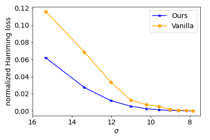
(a) Average over 100 trials: our spectral algorithm outperforms the vanilla algorithm with a smaller error.

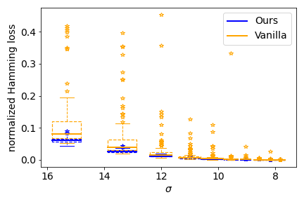
(b) Box plot: our algorithm also has a smaller variance compared to the vanilla method.

Figure 1: Comparisons between our method and the vanilla spectra method on synthetic data.

3 Theoretical Guarantees

In this section, we establish theoretical guarantees for Algorithm 1. Without loss of generality, starting from this part of the paper, we let $Z^{*}_{j}=I_{d}$ for all $j\in[n]$. That is, all the latent permutations are the identity matrix. In this way, the population eigenspace $U^{*}$ has a simpler expression with

$$U^{*}_{j}=I_{d}/\sqrt{n},\forall j\in[n].$$ (10)

To establish the statistical optimality of the proposed method, we first give a justification for the choice of the anchor $M$, followed by a fine-grained perturbation analysis for $U$.

3.1 Theoretical Justification of $M$

We present a justification for the anchor $M$. Note that the empirical eigenspace $U$ and the population eigenspace $U^{*}$ are close modulo a suitable transformation. Readers who are familiar with the literature on spectral methods [1] may recognize that a natural choice of transformation is

$$H:=U^{\top}U^{*}\,.$$ (11)

Classical perturbation theory such as Davis-Kahan theorem can be applied to quantify the distance between $UH$ and $U^{*}$ (see (52) of Lemma 5 for its proof):

$$\left\|{UH-U^{*}}\right\|_{\rm op}\lesssim\frac{{1+\sigma\sqrt{d}}}{\sqrt{np}}.$$

Though $H$ is not orthonormal, it can be shown to be close to some orthogonal matrix (see Lemma 5). Then following the intuition given in Section 2.1 and applying state-of-the-art clustering analysis, we have the following proposition.

Proposition 1.

There exist constants $C_{1},C_{2},C_{3}>0$ such that if $\frac{np}{\log n}>C_{1}$ and $\frac{np}{(\sqrt{d}+\sigma d)^{2}}>C_{2}$ then the anchor $M$ constructed in Algorithm 1 satisfies

$$\min_{P\in\Pi_{d}}\left\|{M-PH^{\top}}\right\|_{\rm F}\leq\frac{C_{3}(\sqrt{d}+\sigma d)}{\sqrt{np}},$$ (12)

with probability at least $1-n^{-10}$.

Proposition 1 shows that $M$ is an approximation of $H^{\top}$ up to some permutation matrix $\hat{P}:=\mathop{\rm argmin}_{P\in\Pi_{d}}\|M-PH^{\top}\|_{\rm F}$. The existence of $\hat{P}$ is due to the fact that the clusters are identifiable only up to a permutation in cluster analysis. (12) shows the estimation error goes to 0 when $\frac{np}{(\sqrt{d}+\sigma d)^{2}}$ grows. As a comparison, the operator norm of the matrix $H$ is ‘of a constant order’ as it is close to an orthogonal matrix. Hence, the error incurred by $M$ as an estimate of $H^{\top}$ is of diminishing proportion. It is also worth mentioning that Proposition 1 holds under weaker assumptions compared to Theorem 1. It only requires $np\gtrsim\log n$ and allows $d$ to grow as long as $np\gtrsim(\sqrt{d}+\sigma d)^{2}$. With Proposition 1, we can have a decomposition of the quantity $U_{j}M^{\top}$, the key quantity in the proposed method (8):

$$U_{j}M^{\top}-U_{j}^{*}\hat{P}^{\top} =U_{j}(\hat{P}H^{\top}+M-\hat{P}H^{\top})^{\top}-U_{j}^{*}\hat{P}^{\top}$$

$$=\left(U_{j}H-U_{j}^{*}\right)\hat{P}^{\top}+U_{j}(M-\hat{P}H^{\top})^{\top}$$

$$\approx\left(U_{j}H-U_{j}^{*}\right)\hat{P}^{\top}.$$ (13)

The approximation (13) is due to (12) as the term above $U_{j}(M-\hat{P}H^{\top})^{\top}$ turns out to be negligible. Hence, the difference $U_{j}M^{\top}-U_{j}^{*}\hat{P}^{\top}$ is primarily about the perturbation $U_{j}H-U_{j}^{*}$. To analyze our spectral method, we need to have a deep understanding on the behaviors of the blockwise perturbation $U_{j}H-U_{j}^{*}$.

3.2 Statistical Optimality

In Theorem 2, we first derive a block-wise $\ell_{\infty}$ upper bound for $UH-U^{*}$, i.e., an upper bound for $\|{U_{j}H-U^{*}_{j}}\|_{\rm op}$ that holds uniformly across all $j\in[n]$.

Theorem 2.

There exist constants $C,C^{\prime},C^{\prime\prime}>0$ such that if $\frac{np}{(\sigma^{4/3}\vee 1)\log n}>C$ and $\frac{np}{(\sqrt{d}+\sigma d)^{2}}\geq C^{\prime}$, we have

$$\max_{j\in[n]}\left\|{U_{j}H-U^{*}_{j}}\right\|_{\rm op}\leq\frac{C^{\prime\prime}}{\sqrt{n}}\left(\sqrt{\frac{\log n}{np}}+\frac{\sigma\sqrt{d}}{\sqrt{np}}+\frac{\sigma\sqrt{\log n}}{\sqrt{np}}\right)$$ (14)

with probability at least $1-6dn^{-9}$.

The upper bound in (14) is equal to the upper bound on $\left\|{UH-U^{*}}\right\|_{\rm op}$ (see Equation (52)) multiplied by a $\sqrt{(\log n)/n}$ factor. This is because $UH-U^{*}$ consists of $n$ blocks $\{U_{j}H-U^{*}\}_{j\in[n]}$ and all blocks behave similarly. The magnitude of each block is then on average $1/\sqrt{n}$ of that of the whole matrix, and the $\sqrt{\log n}$ factor is due to the use of union bound to control the supreme. Theorem 2 assumes $\frac{np}{(\sigma^{4/3}\vee 1)\log n}\gtrsim 1$. A sufficient condition is ${np}/{\log^{3}n}\gtrsim 1$ as $np/\sigma^{2}\gtrsim 1$ is implied by the other assumption ${np}/{(\sqrt{d}+\sigma d)^{2}}\gtrsim 1$.

With the upper bound for each $\|{U_{j}H-U^{*}_{j}}\|_{\rm op}$ derived, we further study the tail behavior of each difference $U_{j}H-U^{*}_{j}$. This leads to a sharp theoretical analysis of the performance of the proposed spectral method. The main theoretical result of this paper is stated below in Theorem 3.

Theorem 3.

Assume $2\leq d\leq\bar{C}$ for some constant $\bar{C}>0$. There exist constants $\bar{C}^{\prime},\bar{C}^{\prime\prime},\bar{C}^{\prime\prime\prime}>0$ such that if $\frac{np}{\log^{3}n}>\bar{C}^{\prime}$ , $\frac{np}{\sigma^{2}}>\bar{C}^{\prime\prime}$ then the estimates $\hat{Z}_{1},\ldots,\hat{Z}_{n}$ of Algorithm 1 satisfy

$$\mathbb{E}\ell(\hat{Z},Z^{*})\leq\exp\left(-\left(1-\bar{C}^{\prime\prime\prime}\left(\left(\frac{\sigma^{2}}{np}\right)^{\frac{1}{4}}+\left(\frac{1}{\log n}\right)^{\frac{1}{4}}\right)\right)\frac{np}{2\sigma^{2}}\right)+n^{-8}.$$

Theorem 3 is a non-asymptotic version of Theorem 1 stated in the Introduction. By letting $np/\sigma^{2}$ go to infinity, the exponential term in Theorem 3 takes an asymptotic form of $\exp\left(-(1-o(1))\frac{np}{2\sigma^{2}}\right)$ and matches with the minimax lower bound. In this way, we establish the statistical optimality of the proposed spectral method.

While the proof of Theorem 3 is complicated, one can still develop an intuition as to why we can achieve the error bound $\exp\left(-(1-o(1))\frac{np}{2\sigma^{2}}\right)$. At a high level, we will prove and use a variant of the linear approximation [1] $UH-U^{*}\approx XU^{*}\Lambda^{-1}-U^{*}$ where $\Lambda$ is the diagonal matrix of the leading eigenvalues of $X$ (see (17)). A further decomposition using the structure of $X$ reveals that

$$U_{j}H-U_{j}^{*}\approx\frac{\sigma}{\sqrt{n}}\,\sum_{k\neq j}A_{jk}W_{jk}\Lambda^{-1}\approx\frac{1}{\sqrt{n}}\frac{\sigma}{np}\sum_{k\neq j}A_{jk}W_{jk}.$$ (15)

Recall that $U_{j}^{*}=I_{d}/\sqrt{n}$ according to (10). Then $\sqrt{n}U_{j}H-I_{d}\approx\frac{\sigma}{np}\sum_{k\neq j}A_{jk}W_{jk}$ which follows a Gaussian distribution conditioned on $\{A_{jk}\}_{k\neq j}$. Since $\sum_{k\neq j}A_{jk}$ concentrates around $(n-1)p$, roughly speaking, $\sqrt{n}U_{j}H-I_{d}$ is a random matrix with each entry i.i.d. following $\mathcal{N}(0,\frac{\sigma^{2}}{np})$. The Gaussian tail is used to characterize the probability of the event when $\sqrt{n}U_{j}H$ considerably deviates away from $I_{d}$ and eventually leads to a probability bound of $\exp\left(-(1-o(1))\frac{np}{2\sigma^{2}}\right)$.

3.3 Block-wise Decomposition of $UH-U^{*}$

In this section, we provide a block-wise decomposition of $UH-U^{*}$. The decomposition is the key towards the block-wise analysis in Section 3.2 and provides insights on how Theorem 2 and Theorem 3 are established. Recall that we let $Z^{*}_{j}=I_{d}$ for all $j\in[n]$. Then, (4) becomes

$$X=(A\otimes I_{d})+\sigma(A\otimes J_{d})\circ W.$$

For each $j\in[n]$, define $X_{j}:=(X_{j1},\ldots,X_{jn})\in\mathbb{R}^{d\times nd}$ to be the $j$-th block row of $X$ and define $W_{j}\in\mathbb{R}^{d\times nd}$ analogously for $W$. Then we have

$$X_{j}=(A_{j}\otimes I_{d})+\sigma(A_{j}\otimes J_{d})\circ W_{j}.$$ (16)

As a result, $X=(X_{1}^{\top},\ldots,X_{n}^{\top})^{\top}$. Define $\Lambda\in\mathbb{R}^{d\times d}$ to be the diagonal matrix of the leading eigenvalues of $X$. That is, $\Lambda_{ii}:=\lambda_{i}(X)$ and $\Lambda_{ik}:=0$ for all $1\leq i\neq k\leq d$. Then we have

$$UH\Lambda-XU^{*} =U(H\Lambda-\Lambda H)+U\Lambda H-XU^{*}$$

$$=U(H\Lambda-\Lambda H)+XUH-XU^{*}$$

$$=U(H\Lambda-\Lambda H)+X(UH-U^{*}).$$

Multiplying both sides by $\Lambda^{-1}$ and rearranging the terms, we have

$$UH-U^{*}=U(H\Lambda-\Lambda H)\Lambda^{-1}+X(UH-U^{*})\Lambda^{-1}+XU^{*}\Lambda^{-1}-U^{*}.$$ (17)

The above display involves $X(UH-U^{*})$ where $X$ and $UH-U^{*}$ are dependent on each other. To decouple the dependence, we approximate $UH-U^{*}$ by its leave-one-out counterparts. Consider any $j\in[n]$. Define $X^{(j)}\in\mathbb{R}^{nd\times nd}$ such that

$$X^{(j)}_{ik}:=\quad\begin{cases}X_{ik},&\forall i,k\neq j,\\ 0_{d\times d},&\text{otherwise.}\end{cases}$$

In addition, let $U^{(j)}\in\mathbb{R}^{nd\times d}$ be the matrix including the leading $d$ eigenvectors of $X^{(j)}$. As a consequence, $X^{(j)},U^{(j)}$ are independent of $\{A_{jk}\}_{k\neq j}$ and $\{W_{jk}\}_{k\neq j}$. Define $H^{(j)}:=U^{(j)\top}U^{*}\in\mathbb{R}^{d\times d}.$ Then

$$UH-U^{*} =UH-U^{(j)}H^{(j)}+U^{(j)}H^{(j)}-U^{*}=(UU^{\top}-U^{(j)}U^{(j)\top})U^{*}+U^{(j)}H^{(j)}-U^{*}.$$

After plugging it into the right-hand side of (17), we have

$$UH-U^{*} =U(H\Lambda-\Lambda H)\Lambda^{-1}+X(UU^{\top}-U^{(j)}U^{(j)\top})U^{*}\Lambda^{-1}$$

$$\quad+X(U^{(j)}H^{(j)}-U^{*})\Lambda^{-1}+XU^{*}\Lambda^{-1}-U^{*}.$$

Then, the $j$th block matrix of $UH-U^{*}$ satisfies

$$U_{j}H-U^{*}_{j} =\underbrace{U_{j}(H\Lambda-\Lambda H)\Lambda^{-1}+X_{j}(UU^{\top}-U^{(j)}U^{(j)\top})U^{*}\Lambda^{-1}}_{=:B_{j}}$$

$$\quad+X_{j}(U^{(j)}H^{(j)}-U^{*})\Lambda^{-1}+X_{j}U^{*}\Lambda^{-1}-U^{*}_{j}.$$ (18)

The last two terms in (18) can be further decomposed. Using (16), we have

$$X_{j}(U^{(j)}H^{(j)}-U^{*})\Lambda^{-1} =\left((A_{j}\otimes I_{d})+\sigma(A_{j}\otimes J_{d})\circ W_{j}\right)(U^{(j)}H^{(j)}-U^{*})\Lambda^{-1}$$

$$=\underbrace{\sum_{k\neq j}A_{jk}(U^{(j)}_{k}H^{(j)}-U^{*}_{k})\Lambda^{-1}}_{=:F_{j1}}+\underbrace{\sigma\sum_{k\neq j}A_{jk}W_{jk}(U^{(j)}_{k}H^{(j)}-U^{*}_{k})\Lambda^{-1}}_{=:F_{j2}},$$

and

$$X_{j}U^{*}\Lambda^{-1}-U^{*}_{j} =\left((A_{j}\otimes I_{d})+\sigma(A_{j}\otimes J_{d})\circ W_{j}\right)U^{*}\Lambda^{-1}-U^{*}_{j}$$

$$=\left(\sum_{k\neq j}A_{jk}U^{*}_{k}\right)\Lambda^{-1}-U_{j}^{*}+\sigma\,\sum_{k\neq j}A_{jk}W_{jk}U^{*}_{k}\Lambda^{-1}$$

$$=\underbrace{\frac{1}{\sqrt{n}}\left(\left(\sum_{k\neq j}A_{jk}\right)\Lambda^{-1}-I_{d}\right)}_{=:G_{j1}}+\underbrace{\frac{\sigma}{\sqrt{n}}\,\sum_{k\neq j}A_{jk}W_{jk}\Lambda^{-1}}_{=:G_{j2}},$$

where the last equation is due to Lemma 4. As a result, we have a decomposition of $U_{j}H-U^{*}_{j}$

$$U_{j}H-U^{*}_{j} =B_{j}+F_{j1}+F_{j2}+G_{j1}+G_{j2},$$ (19)

holds for all $j\in[n]$.

The block-wise decomposition (19) of $UH-U^{*}$ is the starting point to establishing both Theorem 2 and Theorem 3. Note that we have a mutual independence among $\{A_{jk}\}_{k\neq i}$, $\{W_{jk}\}_{k\neq i}$, and $U^{(j)}H^{(j)}-U^{*}$ in the definitions of $F_{j1}$ and $F_{j2}$, which is crucial to obtaining sharp bounds and tail probabilities for them. Theorem 2 is proved by establishing upper bounds for the operator norm of $B_{j},F_{j1},F_{j2},G_{j1}$, and $G_{j2}$. By further analyzing their tail bounds, we establish Theorem 3. Among these terms, $G_{j2}$ is the one contributing to the exponential error bound in Theorem 3, as we illustrate in (15).

4 Proofs

4.1 Proof of Proposition 1

We first state and prove a deterministic version of Proposition 1. The proof of Proposition 1 follows from a simple probabilistic argument.

Lemma 1.

Assume that (52) holds. If $\frac{np}{(\sqrt{d}+\sigma d)^{2}}\geq 32C_{0}^{2}$, we have

$$\min_{P\in\Pi_{d}}\left\|{M-PH^{\top}}\right\|_{\rm F}\leq\frac{{4C_{0}\left(\sqrt{d}+\sigma d\right)}}{\sqrt{np}}.$$ (20)

Proof.

Note that

$$\left\|{U-U^{*}H^{\top}}\right\|_{\rm op} =\left\|{UU^{\top}U-U^{*}U^{*\top}U}\right\|_{\rm op}\leq\left\|{UU^{\top}-U^{*}U^{*\top}}\right\|_{\rm op}\left\|{U}\right\|_{\rm op}\leq\left\|{UU^{\top}-U^{*}U^{*\top}}\right\|_{\rm op}.$$

Since (52) holds, we have

$$\left\|{U-U^{*}H^{\top}}\right\|_{\rm F} \leq\sqrt{d}\left\|{U-U^{*}H^{\top}}\right\|_{\rm op}\leq\sqrt{d}\frac{8C_{0}\left(1+\sigma\sqrt{d}\right)}{7\sqrt{np}}.$$

Note that $\sqrt{n}U^{*}$ has only $k$ unique rows $e_{1}^{\top},\ldots,e_{d}^{\top}$ and each is of size $n$. Then $\sqrt{n}U^{*}H^{\top}$ also has $k$ unique rows $e_{1}^{\top}H^{\top},\ldots,e_{d}^{\top}H^{\top}$ and each is of size $n$. From (52), there exists a matrix $O\in\mathcal{O}_{d}$ such that $\left\|{H-O}\right\|_{\rm op}\leq\frac{8C_{0}\left(1+\sigma\sqrt{d}\right)}{7\sqrt{np}}\leq\frac{1}{7}$. Then

$$\min_{a,b\in[d]}\left\|{(e_{a}-e_{b})^{\top}H^{\top}}\right\| \geq\min_{a,b\in[d]}\left\|{(e_{a}-e_{b})^{\top}\left(O^{\top}+(H-O)^{\top}\right)}\right\|$$

$$\geq\min_{a,b\in[d]}\left\|{(e_{a}-e_{b})^{\top}O^{\top}}\right\|-\left\|{H-O}\right\|_{\rm op}$$

$$\geq\sqrt{2}-\frac{1}{7}$$

$$\geq\frac{6}{5}.$$

That is, $\Delta$, defined as the minimum distance among the unique rows of $U^{*}H^{\top}$, is at least $\frac{6}{5\sqrt{n}}$.

Let $\hat{z}\in[d]^{nd}$ be the minimizer of (7) with $\{\hat{\mu}_{1},\ldots,\hat{\mu}_{d}\}$. Denote $\hat{\Theta}:=(\hat{\mu}_{\hat{z}_{1}}^{\top},\ldots,\hat{\mu}_{\hat{z}_{nd}}^{\top})^{\top}\in\mathbb{R}^{nd\times d}$. According to (7), we have $\left\|{\hat{\Theta}-U}\right\|_{\rm F}\leq\left\|{U^{*}H^{\top}-U}\right\|_{\rm F}$. Hence,

$$\left\|{\hat{\Theta}-U^{*}H^{\top}}\right\|_{\rm F} \leq\left\|{\hat{\Theta}-U}\right\|_{\rm F}+\left\|{U^{*}H^{\top}-U}\right\|_{\rm F}\leq 2\left\|{U-U^{*}H^{\top}}\right\|_{\rm F}\leq\sqrt{d}\frac{16C_{0}\left(1+\sigma\sqrt{d}\right)}{7\sqrt{np}}.$$

Define $z^{*}\in[d]^{nd}$ such that the $i$th row of $U^{*}H^{\top}$ is equal to $e_{z^{*}_{i}}^{\top}H^{T}/\sqrt{n}$ for each $i\in[n]$. Define the set $S$ as

$$S:=\left\{i\in[nd]:\left\|{\hat{\mu}_{\hat{z}_{i}}-e_{z^{*}_{i}}^{\top}H^{T}/\sqrt{n}}\right\|>\frac{\Delta}{2}\right\}.$$

Then we have

$$\left|S\right|\leq\frac{\left\|{\hat{\Theta}-U^{*}H^{\top}}\right\|_{\rm F}^{2}}{(\Delta/2)^{2}}\leq\frac{\left(4C_{0}\left(\sqrt{d}+\sigma d\right)\right)^{2}}{p}$$

Under the assumption $\frac{np}{(\sqrt{d}+\sigma d)^{2}}\geq 32C_{0}^{2},$ we have $\left|S\right|\leq n/2$. Then by the same argument as in the proof of Proposition 3.1 of [22], there exists a bijection $\phi:[d]\rightarrow[d]$ such that $\hat{z}_{i}=\phi(z^{*}_{i})$ for all $i\notin S$. Hence, for each $a\in[d]$, we have

$$\left\|{\hat{\mu}_{\phi(a)}-e_{a}^{\top}H^{\top}/\sqrt{n}}\right\|^{2} =\frac{\sum_{i\in[nd]:\hat{z}_{i}=\phi(a),z^{*}_{i}=a}\left\|{\hat{\mu}_{\hat{z}_{i}}-e_{z^{*}_{i}}^{\top}H^{\top}}\right\|^{2}}{\left|i\in[nd]:\hat{z}_{i}=\phi(a),z^{*}_{i}=a\right|}\leq\frac{\sum_{i\in[nd]:\hat{z}_{i}=\phi(a)}\left\|{\hat{\mu}_{\hat{z}_{i}}-e_{z^{*}_{i}}^{\top}H^{\top}}\right\|^{2}}{n-\left|S\right|}$$

$$\leq\frac{\sum_{i\in[nd]:\hat{z}_{i}=\phi(a)}\left\|{\hat{\mu}_{\hat{z}_{i}}-e_{z^{*}_{i}}^{\top}H^{\top}}\right\|^{2}}{n/2}.$$

Hence,

$$\sum_{a\in[d]}\left\|{\hat{\mu}_{\phi(a)}-e_{a}^{\top}H^{\top}/\sqrt{n}}\right\|^{2}\leq\frac{\sum_{i\in[nd]}\left\|{\hat{\mu}_{\hat{z}_{i}}-e_{z^{*}_{i}}^{\top}H^{\top}}\right\|^{2}}{n/2}=\frac{\left\|{\hat{\Theta}-U^{*}H^{\top}}\right\|_{\rm F}^{2}}{n/2}\leq\frac{\left(4C_{0}\left(\sqrt{d}+\sigma d\right)\right)^{2}}{n^{2}p}.$$

That is, there exists a permutation matrix $P$ such that

$$\left\|{M-PH^{\top}}\right\|_{\rm F}^{2}\leq\frac{\left(4C_{0}\left(\sqrt{d}+\sigma d\right)\right)^{2}}{np},$$

since rows of $M$ are $\sqrt{n}\hat{\mu}_{1},\ldots,\sqrt{n}\hat{\mu}_{d}$. ∎

Proof of Proposition 1.

According to Lemma 5, there exist constants $C,C_{0}>0$ such that if $\frac{np}{\log n}>C$ and $\frac{np}{(1+\sigma\sqrt{d})^{2}}\geq 64C_{0}^{2}$, we have (52) hold with probability at least $1-n^{-10}$. The proof is complete by Lemma 1. ∎

4.2 Proof of Theorem 2

We first give a deterministic upper bound for $\|{U_{j}H-U^{*}_{j}}\|_{\rm op}$, using the decomposition (19).

Lemma 2.

Assume (47)-(58) hold. Under the assumption $\frac{np}{(1+\sigma\sqrt{d})^{2}}\geq 22^{2}C_{0}^{2}$, for each $j\in[n]$, we have

$$\left\|{U_{j}H-U^{*}_{j}}\right\|_{\rm op} \leq\frac{22C_{0}}{\sqrt{n}}\left(\frac{1+\sigma\sqrt{d}}{\sqrt{np}}\right)+2\left\|{F_{j1}}\right\|_{\rm op}+2\left\|{F_{j2}}\right\|_{\rm op}+2\left\|{G_{j1}}\right\|_{\rm op}+2\left\|{G_{j2}}\right\|_{\rm op},$$ (21)

and

$$\left\|{B_{j}}\right\|_{\rm op} \leq 22C_{0}\left(\frac{1}{\sqrt{n}}+\left\|{F_{j1}}\right\|_{\rm op}+\left\|{F_{j2}}\right\|_{\rm op}+\left\|{G_{j1}}\right\|_{\rm op}+\left\|{G_{j2}}\right\|_{\rm op}\right)\left(\frac{1+\sigma\sqrt{d}}{\sqrt{np}}\right).$$ (22)

Proof.

Consider any $j\in[n]$. We have

$$\left\|{B_{j}}\right\|_{\rm op} \leq\left\|{U_{j}}\right\|_{\rm op}\left\|{H\Lambda-\Lambda H}\right\|_{\rm op}\left\|{\Lambda^{-1}}\right\|_{\rm op}+\left\|{X_{j}}\right\|_{\rm op}\left\|{UU^{\top}-U^{(j)}U^{(j)\top}}\right\|_{\rm op}\left\|{\Lambda^{-1}}\right\|_{\rm op}$$

$$\leq{\frac{4}{3}\left(\left\|{U_{j}H-U^{*}_{j}}\right\|_{\rm op}+\frac{1}{\sqrt{n}}\right)}\left(2C_{0}\left(1+\sigma\sqrt{d}\right)\sqrt{np}\right)\frac{8}{7np}$$

$$\quad+\left(p\sqrt{n}+C_{0}\left(1+\sigma\sqrt{d}\right)\sqrt{np}\right)\left(6\left(\left\|{U_{j}H-U^{*}_{j}}\right\|_{\rm op}+\frac{1}{\sqrt{n}}\right)\right)\frac{8}{7np}$$

$$\leq\frac{8}{7np}\left(\left\|{U_{j}H-U^{*}_{j}}\right\|_{\rm op}+\frac{1}{\sqrt{n}}\right)\left(6p\sqrt{n}+\frac{26}{3}C_{0}\left(1+\sigma\sqrt{d}\right)\sqrt{np}\right)$$

$$\leq 11C_{0}\left(\left\|{U_{j}H-U^{*}_{j}}\right\|_{\rm op}+\frac{1}{\sqrt{n}}\right)\left(\frac{1+\sigma\sqrt{d}}{\sqrt{np}}\right),$$

where the second inequality is by (47)-(58) and the last inequality is by $C_{0}>7$. From (19), we also have

$$\left\|{U_{j}H-U^{*}_{j}}\right\|_{\rm op} \leq\left\|{B_{j}}\right\|_{\rm op}+\left\|{F_{j1}}\right\|_{\rm op}+\left\|{F_{j2}}\right\|_{\rm op}+\left\|{G_{j1}}\right\|_{\rm op}+\left\|{G_{j2}}\right\|_{\rm op}.$$

Plug the upper bound (22) of $\left\|{B_{j}}\right\|_{\rm op}$ into the above display. After rearrangement, we have

$$\left(1-11C_{0}\left(\frac{1+\sigma\sqrt{d}}{\sqrt{np}}\right)\right)\left\|{U_{j}H-U^{*}_{j}}\right\|_{\rm op} \leq\frac{11C_{0}}{\sqrt{n}}\left(\frac{1+\sigma\sqrt{d}}{\sqrt{np}}\right)+\left\|{F_{j1}}\right\|_{\rm op}+\left\|{F_{j2}}\right\|_{\rm op}+\left\|{G_{j1}}\right\|_{\rm op}+\left\|{G_{j2}}\right\|_{\rm op}.$$

Under the assumption $\frac{np}{(1+\sigma\sqrt{d})^{2}}\geq 22^{2}C_{0}^{2}$, we have

$$\left\|{U_{j}H-U^{*}_{j}}\right\|_{\rm op} \leq\frac{22C_{0}}{\sqrt{n}}\left(\frac{1+\sigma\sqrt{d}}{\sqrt{np}}\right)+2\left\|{F_{j1}}\right\|_{\rm op}+2\left\|{F_{j2}}\right\|_{\rm op}+2\left\|{G_{j1}}\right\|_{\rm op}+2\left\|{G_{j2}}\right\|_{\rm op}.$$

Plugging it into the upper bound of $\left\|{B_{j}}\right\|_{\rm op}$, we have

$$\left\|{B_{j}}\right\|_{\rm op} \leq 11C_{0}\left(\left(\frac{22C_{0}}{\sqrt{n}}\left(\frac{1+\sigma\sqrt{d}}{\sqrt{np}}\right)+2\left\|{F_{j1}}\right\|_{\rm op}+2\left\|{F_{j2}}\right\|_{\rm op}+2\left\|{G_{j1}}\right\|_{\rm op}+2\left\|{G_{j2}}\right\|_{\rm op}\right)+\frac{1}{\sqrt{n}}\right)\left(\frac{1+\sigma\sqrt{d}}{\sqrt{np}}\right)$$

$$\leq 22C_{0}\left(\frac{1}{\sqrt{n}}+\left\|{F_{j1}}\right\|_{\rm op}+\left\|{F_{j2}}\right\|_{\rm op}+\left\|{G_{j1}}\right\|_{\rm op}+\left\|{G_{j2}}\right\|_{\rm op}\right)\left(\frac{1+\sigma\sqrt{d}}{\sqrt{np}}\right).$$

∎

As a preview, the terms $\left\|{F_{j1}}\right\|_{\rm op}$, $\left\|{F_{j2}}\right\|_{\rm op}$, $\left\|{G_{j1}}\right\|_{\rm op}$ and $\left\|{G_{j2}}\right\|_{\rm op}$ in (21) and (22) can be bounded using the helper Lemma 6, Lemma 7, Lemma 8 and Lemma 10 respectively. We defer the proof of these helper lemmas to a later section. To shorten the notation, let us denote

$$\Delta:=UH-U^{*}\in\mathbb{R}^{nd\times d},\quad\Delta^{(j)}:=U^{(j)}H^{(j)}-U^{*}\in\mathbb{R}^{nd\times d},\forall j\in[n],$$ (23)

such that block submatrices $\Delta_{k}=U_{k}H-U^{*}_{k}$ and $\Delta^{(j)}_{k}=U^{(j)}_{k}H^{(j)}-U^{*}_{k}$ for each $j,k\in[n]$. We further introduce $\left\|{\cdot}\right\|_{\rm op,\infty}$ norm such that

$$\left\|{\Delta}\right\|_{\rm op,\infty} :=\max_{k\in[n]}\left\|{\Delta_{k}}\right\|_{\rm op},\quad\left\|{\Delta^{(j)}}\right\|_{\rm op,\infty}:=\max_{k\in[n]}\left\|{\Delta^{(j)}_{k}}\right\|_{\rm op}.$$ (24)

They are related as shown below in Lemma 3.

Lemma 3.

Assume (57) holds. Then for any $j\in[n]$, we have

$$\left\|{\Delta^{(j)}}\right\|_{\rm op,\infty} \leq 7\left(\left\|{\Delta}\right\|_{\rm op,\infty}+\frac{1}{\sqrt{n}}\right).$$ (25)

Proof.

Consider any $j\in[n]$, we have

$$\left\|{\Delta^{(j)}}\right\|_{\rm op,\infty} \leq\left\|{\Delta}\right\|_{\rm op,\infty}+\left\|{\Delta-\Delta^{(j)}}\right\|_{\rm op,\infty}\leq\left\|{\Delta}\right\|_{\rm op,\infty}+\left\|{\Delta-\Delta^{(j)}}\right\|_{\rm op}$$

$$=\left\|{\Delta}\right\|_{\rm op,\infty}+\left\|{UH-U^{(j)}H^{(j)}}\right\|_{\rm op}=\left\|{\Delta}\right\|_{\rm op,\infty}+\left\|{UU^{\top}U^{*}-U^{(j)}U^{(j)\top}U^{*}}\right\|_{\rm op}$$

$$\leq\left\|{\Delta}\right\|_{\rm op,\infty}+\left\|{UU^{\top}-U^{(j)}U^{(j)\top}}\right\|_{\rm op}\leq\left\|{\Delta}\right\|_{\rm op,\infty}+6\left(\left\|{U_{j}H-U^{*}_{j}}\right\|_{\rm op}+\frac{1}{\sqrt{n}}\right)$$

$$\leq 7\left(\left\|{\Delta}\right\|_{\rm op,\infty}+\frac{1}{\sqrt{n}}\right),$$

where the second to last inequality is due to (57). ∎

We are now ready to prove Theorem 2.

Proof of Theorem 2.

From Lemma 5, there exist constants $C_{0}^{\prime},C_{0}>0$ such that if $\frac{np}{\log n}>C_{0}^{\prime}$, then the event $\mathcal{E}$ holds with probability at least $1-n^{-10}$. Assume $\mathcal{E}$ holds and $\frac{np}{(\sqrt{d}+\sigma d)^{2}}\geq 22^{2}C_{0}^{2}$. Then according to Lemma 5, we have (47)-(58) hold. As a consequence, by Lemma 2 and Lemma 3, we have (21) and (25) all hold as well.

Consider any $j\in[n]$. Note that (21) can be written as

$$\left\|{\Delta_{j}}\right\|_{\rm op} \leq\frac{22C_{0}}{\sqrt{n}}\left(\frac{1+\sigma\sqrt{d}}{\sqrt{np}}\right)+2\left\|{F_{j1}}\right\|_{\rm op}+2\left\|{F_{j2}}\right\|_{\rm op}+2\left\|{G_{j1}}\right\|_{\rm op}+2\left\|{G_{j2}}\right\|_{\rm op}.$$ (26)

Hence, to upper bound $\left\|{\Delta_{j}}\right\|_{\rm op}$, we need to study $\left\|{F_{j1}}\right\|_{\rm op}$, $\left\|{F_{j2}}\right\|_{\rm op}$, $\left\|{G_{j1}}\right\|_{\rm op}$, and $\left\|{G_{j2}}\right\|_{\rm op}$. By Lemma 6, we have

$$\left\|{\sum_{k\neq j}A_{jk}\Delta_{k}^{(j)}}\right\|_{\rm op} \leq p\sqrt{n}\left\|{\Delta^{(j)}}\right\|_{\rm op}+\sqrt{40np\left\|{\Delta^{(j)}}\right\|_{\rm op,\infty}^{2}\log n}+\frac{40}{3}\log n\left\|{\Delta^{(j)}}\right\|_{\rm op,\infty}$$

$$\leq p\sqrt{n}\left\|{\Delta^{(j)}}\right\|_{\rm op}+\left(\sqrt{40np\log n}+\frac{40}{3}\log n\right)\left\|{\Delta^{(j)}}\right\|_{\rm op,\infty},$$

holds with probability at least $1-2dn^{-10}$. Then with (50), we have

$$\left\|{F_{j1}}\right\|_{\rm op} \leq\left\|{\sum_{k\neq j}A_{jk}\Delta_{k}^{(j)}}\right\|_{\rm op}\left\|{\Lambda^{-1}}\right\|_{\rm op}$$

$$\leq\frac{8}{7np}\left(p\sqrt{n}\left\|{\Delta^{(j)}}\right\|_{\rm op}+\left(\sqrt{40np\log n}+\frac{40}{3}\log n\right)\left\|{\Delta^{(j)}}\right\|_{\rm op,\infty}\right)$$

$$\leq\frac{C_{1}}{\sqrt{n}}\left\|{\Delta^{(j)}}\right\|_{\rm op}+C_{1}\sqrt{\frac{\log n}{np}}\left\|{\Delta^{(j)}}\right\|_{\rm op,\infty},$$ (27)

for some constant $C_{1}>0$. By Lemma 8, we have

$$\left\|{\sum_{k\neq j}A_{jk}W_{jk}\Delta^{(j)}_{k}}\right\|_{\rm op} \leq C_{2}\sqrt{\log n}\left\|{\sum_{k\neq j}A_{jk}(\Delta^{(j)}_{k})^{\top}\Delta^{(j)}_{k}}\right\|_{\rm op}^{\frac{1}{2}}$$

holds with probability at least $1-n^{-10}$ for some constant $C_{2}>0$. In addition, by Lemma 7, we have

$$\left\|{\sum_{k\neq j}A_{jk}(\Delta^{(j)}_{k})^{\top}\Delta^{(j)}_{k}}\right\|_{\rm op} \leq p\left\|{\Delta^{(j)}}\right\|_{\rm op}^{2}+\sqrt{40p\left\|{\Delta^{(j)}}\right\|_{\rm op}^{2}\left\|{\Delta^{(j)}}\right\|_{\rm op,\infty}^{2}\log n}+\frac{40}{3}\log n\left\|{\Delta^{(j)}}\right\|_{\rm op,\infty}^{2}$$

$$\leq p\left\|{\Delta^{(j)}}\right\|_{\rm op}^{2}+\sqrt{40np\left\|{\Delta^{(j)}}\right\|_{\rm op,\infty}^{4}\log n}+\frac{40}{3}\log n\left\|{\Delta^{(j)}}\right\|_{\rm op,\infty}^{2}$$

$$\leq p\left\|{\Delta^{(j)}}\right\|_{\rm op}^{2}+\left(\sqrt{40np\log n}+\frac{40}{3}\log n\right)\left\|{\Delta^{(j)}}\right\|_{\rm op,\infty}^{2}$$

holds with probability at least $1-2dn^{-10}$. Then with (50), we have

$$\left\|{F_{j2}}\right\|_{\rm op} \leq\sigma\left\|{\sum_{k\neq j}A_{jk}W_{jk}\Delta^{(j)}_{k}}\right\|_{\rm op}\left\|{\Lambda^{-1}}\right\|_{\rm op}$$

$$\leq\frac{8\sigma}{7np}C_{2}\sqrt{\log n}\sqrt{p\left\|{\Delta^{(j)}}\right\|_{\rm op}^{2}+\left(\sqrt{40np\log n}+\frac{40}{3}\log n\right)\left\|{\Delta^{(j)}}\right\|_{\rm op,\infty}^{2}}$$

$$\leq\frac{8\sigma}{7np}C_{2}\sqrt{\log n}\left(\sqrt{p}\left\|{\Delta^{(j)}}\right\|_{\rm op}+\sqrt{\sqrt{40np\log n}+\frac{40}{3}\log n}\left\|{\Delta^{(j)}}\right\|_{\rm op,\infty}\right)$$

$$\leq\frac{C_{3}\sigma}{\sqrt{n}}\sqrt{\frac{\log n}{np}}\left\|{\Delta^{(j)}}\right\|_{\rm op}+C_{3}\sigma\left(\frac{\log n}{np}\right)^{\frac{3}{4}}\left\|{\Delta^{(j)}}\right\|_{\rm op,\infty},$$ (28)

for some constant $C_{3}>0$. For $\left\|{G_{j1}}\right\|$, its upper bound is given in (55). By Lemma 10, using the fact that $\{A_{ij}\}_{k\neq j}$ and $\{W_{jk}\}_{k\neq j}$ are independent, we have

$$\left\|{\sum_{k\neq j}A_{jk}W_{jk}}\right\|_{\rm op} \leq\sqrt{\sum_{k\neq j}A_{jk}}\left(2\sqrt{d}+C_{4}\sqrt{\log n}\right),$$

with probability at least $1-n^{-10}$, for some constant $C_{4}>0$. Then

$$\left\|{G_{j2}}\right\|_{\rm op} \leq\frac{\sigma}{\sqrt{n}}\left\|{\sum_{k\neq j}A_{jk}W_{jk}}\right\|_{\rm op}\left\|{\Lambda^{-1}}\right\|_{\rm op}$$

$$\leq\frac{\sigma}{\sqrt{n}}\sqrt{\sum_{k\neq j}A_{jk}}\left(2\sqrt{d}+C_{4}\sqrt{\log n}\right)\left\|{\Lambda^{-1}}\right\|_{\rm op}$$

$$\leq C_{5}\frac{\sigma}{\sqrt{n}}\left(\sqrt{\frac{d}{np}}+\sqrt{\frac{\log n}{np}}\right),$$ (29)

for some constant $C_{5}>0$, where the last inequality is by $\mathcal{E}$ and (50).

Plugging (27), (28), (55), and (29) into (26), we have

$$\left\|{\Delta_{j}}\right\|_{\rm op} \leq\frac{22C_{0}}{\sqrt{n}}\left(\frac{1+\sigma\sqrt{d}}{\sqrt{np}}\right)+2\left(\frac{C_{1}}{\sqrt{n}}\left\|{\Delta^{(j)}}\right\|_{\rm op}+C_{1}\sqrt{\frac{\log n}{np}}\left\|{\Delta^{(j)}}\right\|_{\rm op}\right)$$

$$\quad+2\left(\frac{C_{3}\sigma}{\sqrt{n}}\sqrt{\frac{\log n}{np}}\left\|{\Delta^{(j)}}\right\|_{\rm op}+C_{3}\sigma\left(\frac{\log n}{np}\right)^{\frac{3}{4}}\left\|{\Delta^{(j)}}\right\|_{\rm op,\infty}\right)+\frac{4C_{0}}{\sqrt{n}}\left(\sqrt{\frac{\log n}{np}}+\frac{\sigma\sqrt{d}}{\sqrt{np}}\right)$$

$$\quad+2C_{5}\frac{\sigma}{\sqrt{n}}\left(\sqrt{\frac{d}{np}}+\sqrt{\frac{\log n}{np}}\right)$$

$$\leq\frac{2}{\sqrt{n}}\left(C_{1}+C_{3}\sigma\sqrt{\frac{\log n}{np}}\right)\left\|{\Delta^{(j)}}\right\|_{\rm op}+2\left(C_{1}\sqrt{\frac{\log n}{np}}+C_{3}\sigma\left(\frac{\log n}{np}\right)^{\frac{3}{4}}\right)\left\|{\Delta^{(j)}}\right\|_{\rm op,\infty}$$

$$\quad+\frac{26C_{0}+2C_{5}}{\sqrt{n}}\frac{\sqrt{\log n}+\sigma\sqrt{d}+\sigma\sqrt{\log n}}{\sqrt{np}}.$$

By (25) and (58), we can replace the terms $\left\|{\Delta^{(j)}}\right\|_{\rm op}$, $\left\|{\Delta^{(j)}}\right\|_{\rm op,\infty}$ with their respective upper bounds and have

$$\left\|{\Delta_{j}}\right\|_{\rm op} \leq\frac{2}{\sqrt{n}}\left(C_{1}+C_{3}\sigma\sqrt{\frac{\log n}{np}}\right)\frac{9C_{0}(1+\sigma\sqrt{d})}{\sqrt{np}}+14\left(C_{1}\sqrt{\frac{\log n}{np}}+C_{3}\sigma\left(\frac{\log n}{np}\right)^{\frac{3}{4}}\right)\left(\left\|{\Delta}\right\|_{\rm op,\infty}+\frac{1}{\sqrt{n}}\right)$$

$$\quad+\frac{26C_{0}+2C_{5}}{\sqrt{n}}\frac{\sqrt{\log n}+\sigma\sqrt{d}+\sigma\sqrt{\log n}}{\sqrt{np}}.$$

By a union bound, with probability at least $1-6dn^{-9}$, the above display holds for all $j\in[n]$. Then

$$\left\|{\Delta}\right\|_{\rm op,\infty} \leq\frac{2}{\sqrt{n}}\left(C_{1}+C_{3}\sigma\sqrt{\frac{\log n}{np}}\right)\frac{9C_{0}(1+\sigma\sqrt{d})}{\sqrt{np}}+14\left(C_{1}\sqrt{\frac{\log n}{np}}+C_{3}\sigma\left(\frac{\log n}{np}\right)^{\frac{3}{4}}\right)\left(\left\|{\Delta}\right\|_{\rm op,\infty}+\frac{1}{\sqrt{n}}\right)$$

$$\quad+\frac{26C_{0}+2C_{5}}{\sqrt{n}}\frac{\sqrt{\log n}+\sigma\sqrt{d}+\sigma\sqrt{\log n}}{\sqrt{np}}.$$

After a rearrangement, we have

$$\left(1-14\left(C_{1}\sqrt{\frac{\log n}{np}}+C_{3}\sigma\left(\frac{\log n}{np}\right)^{\frac{3}{4}}\right)\right)\left\|{\Delta}\right\|_{\rm op,\infty}$$

$$\leq\frac{2}{\sqrt{n}}\left(C_{1}+C_{3}\sigma\sqrt{\frac{\log n}{np}}\right)\frac{9C_{0}(1+\sigma\sqrt{d})}{\sqrt{np}}+\frac{14}{\sqrt{n}}\left(C_{1}\sqrt{\frac{\log n}{np}}+C_{3}\sigma\left(\frac{\log n}{np}\right)^{\frac{3}{4}}\right)$$

$$\quad+\frac{26C_{0}+2C_{5}}{\sqrt{n}}\frac{\sqrt{\log n}+\sigma\sqrt{d}+\sigma\sqrt{\log n}}{\sqrt{np}}.$$

Then, there exists a constant $C>0$ such that if $\frac{np}{(\sigma^{4/3}\vee 1)\log n}>C$, we have $14\left(C_{1}\sqrt{\frac{\log n}{np}}+C_{3}\sigma\left(\frac{\log n}{np}\right)^{\frac{3}{4}}\right)\leq\frac{1}{2}$. Consequently, we have

$$\left\|{\Delta}\right\|_{\rm op,\infty} \leq\frac{4}{\sqrt{n}}\left(C_{1}+C_{3}\sigma\sqrt{\frac{\log n}{np}}\right)\frac{9C_{0}(1+\sigma\sqrt{d})}{\sqrt{np}}+\frac{28}{\sqrt{n}}\left(C_{1}\sqrt{\frac{\log n}{np}}+C_{3}\sigma\left(\frac{\log n}{np}\right)^{\frac{3}{4}}\right)$$

$$\quad+\frac{52C_{0}+4C_{5}}{\sqrt{n}}\frac{\sqrt{\log n}+\sigma\sqrt{d}+\sigma\sqrt{\log n}}{\sqrt{np}}$$

$$\leq\frac{C_{6}}{\sqrt{n}}\left(\sqrt{\frac{\log n}{np}}+\frac{\sigma\sqrt{d}}{\sqrt{np}}+\frac{\sigma\sqrt{\log n}}{\sqrt{np}}\right),$$

for some constant $C_{6}>0$.

∎

4.3 Proof of Theorem 3

Decomposition of the Hamming loss. From Lemma 5, there exist constants $C_{0}^{\prime},C_{0}>0$ such that if $\frac{np}{\log n}>C_{0}^{\prime}$, then the event $\mathcal{E}$ holds with probability at least $1-n^{-10}$. By Theorem 2, there exist some constants $C,C^{\prime},C^{\prime\prime}>0$ such that if $\frac{np}{(\sigma^{4/3}\vee 1)\log n}>C$ and $\frac{np}{(\sqrt{d}+\sigma d)^{2}}\geq C^{\prime}$, we have (14) holds with probability at least $1-6dn^{-9}$. Denote $\mathcal{F}$ to be the event that both $\mathcal{E}$ and (14) hold. By union bound, we have

$$\mathbb{P}\left(\mathcal{F}\right)\geq 1-7dn^{-9}.$$ (30)

Assume $\mathcal{F}$ holds and $\frac{np}{(\sqrt{d}+\sigma d)^{2}}\geq 22^{2}C_{0}^{2}$. Then according to Lemma 5, we have (47)-(58) hold. As a consequence, by Lemma 2, Lemma 3, and Lemma 1, we have (21), (25), and (20) all hold as well. Since

$$\mathbb{E}\ell(\hat{Z},Z^{*})\leq\mathbb{E}\ell(\hat{Z},Z^{*}){\mathbb{I}\left\{{\mathcal{F}}\right\}}+\mathbb{P}\left(\mathcal{F}^{\mathrm{c}}\right),$$ (31)

in the following we focus on analyzing $\mathbb{E}\ell(\hat{Z},Z^{*}){\mathbb{I}\left\{{\mathcal{F}}\right\}}$.

Define

$$\hat{P}:=\mathop{\rm argmin}_{P\in\Pi_{d}}\,\left\|{M-PH^{\top}}\right\|_{\rm F}.$$

Since we let $Z^{*}_{j}=I_{d}$ for all $j\in[n]$, we have

$$\mathbb{E}\ell(\hat{Z},Z^{*}){\mathbb{I}\left\{{\mathcal{F}}\right\}} \leq\mathbb{E}\left(\frac{1}{n}\sum_{j\in[n]}{\mathbb{I}\left\{{\hat{Z}_{j}\neq Z^{*}_{j}\hat{P}^{\top}}\right\}}{\mathbb{I}\left\{{\mathcal{F}}\right\}}\right)=\frac{1}{n}\sum_{j\in[n]}\mathbb{E}{\mathbb{I}\left\{{\hat{Z}_{j}\neq Z^{*}_{j}\hat{P}^{\top}}\right\}}{\mathbb{I}\left\{{\mathcal{F}}\right\}}$$

$$\leq\frac{1}{n}\sum_{j\in[n]}\mathbb{E}{\mathbb{I}\left\{{\exists R\in\Pi_{d}\text{ s.t. }R\neq I_{d}\text{ and }\left\|{\sqrt{n}U_{j}M^{\top}-R\hat{P}^{\top}}\right\|_{\rm F}^{2}\leq\left\|{\sqrt{n}U_{j}M^{\top}-Z^{*}_{j}\hat{P}^{\top}}\right\|_{\rm F}^{2}}\right\}}{\mathbb{I}\left\{{\mathcal{F}}\right\}}$$

$$=\frac{1}{n}\sum_{j\in[n]}\mathbb{E}{\mathbb{I}\left\{{\exists R\in\Pi_{d}\text{ s.t. }R\neq I_{d}\text{ and }\left\|{U_{j}M^{\top}-\frac{R\hat{P}^{\top}}{\sqrt{n}}}\right\|_{\rm F}^{2}\leq\left\|{U_{j}M^{\top}-U^{*}_{j}\hat{P}^{\top}}\right\|_{\rm F}^{2}}\right\}}{\mathbb{I}\left\{{\mathcal{F}}\right\}}$$

$$\leq\frac{1}{n}\sum_{j\in[n]}\sum_{R\in\Pi_{d}:R\neq I_{d}}\mathbb{E}{\mathbb{I}\left\{{\left\|{U_{j}M^{\top}-\frac{R\hat{P}^{\top}}{\sqrt{n}}}\right\|_{\rm F}^{2}\leq\left\|{U_{j}M^{\top}-U^{*}_{j}\hat{P}^{\top}}\right\|_{\rm F}^{2}}\right\}}{\mathbb{I}\left\{{\mathcal{F}}\right\}},$$ (32)

where the second inequity is by the definition of $\hat{Z}_{j}$ in (6) and the second equation is by that we let $Z^{*}_{j}=I_{d}$.

Consider any $R\in\Pi_{d}$ such that $R\neq I_{d}$. Define

$$h_{R}:=\left\|{R-I_{d}}\right\|_{\rm F}^{2}/2.$$

Then $2\leq h_{R}\leq d$. Consider any $j\in[n]$. In the following, we are going to establish an upper bound for $\mathbb{E}{\mathbb{I}\left\{{\left\|{U_{j}M^{\top}-\frac{R\hat{P}^{\top}}{\sqrt{n}}}\right\|_{\rm F}^{2}\leq\left\|{U_{j}M^{\top}-U^{*}_{j}\hat{P}^{\top}}\right\|_{\rm F}^{2}}\right\}}{\mathbb{I}\left\{{\mathcal{F}}\right\}}$, the key quantity in (32).

We have

$${\mathbb{I}\left\{{\left\|{U_{j}M^{\top}-U_{j}^{*}\hat{P}^{\top}}\right\|_{\rm F}\geq\left\|{U_{j}M^{\top}-\frac{R\hat{P}^{\top}}{\sqrt{n}}}\right\|_{\rm F}}\right\}}{\mathbb{I}\left\{{\mathcal{F}}\right\}}$$

$$={\mathbb{I}\left\{{\left\langle U_{j}M^{\top}-U_{j}^{*}\hat{P}^{\top},\frac{R\hat{P}^{\top}}{\sqrt{n}}-U_{j}^{*}\hat{P}^{\top}\right\rangle\geq\frac{1}{2}\left\|{\frac{R\hat{P}^{\top}}{\sqrt{n}}-U_{j}^{*}\hat{P}^{\top}}\right\|_{\rm F}^{2}}\right\}}{\mathbb{I}\left\{{\mathcal{F}}\right\}}$$

$$={\mathbb{I}\left\{{\left\langle U_{j}M^{\top}\hat{P}-U_{j}^{*},\frac{R}{\sqrt{n}}-U_{j}^{*}\right\rangle\geq\frac{1}{2}\left\|{\frac{R}{\sqrt{n}}-U_{j}^{*}}\right\|_{\rm F}^{2}}\right\}}{\mathbb{I}\left\{{\mathcal{F}}\right\}}$$

$$={\mathbb{I}\left\{{\left\langle U_{j}M^{\top}\hat{P}-U_{j}^{*},R-I_{d}\right\rangle\geq\frac{h_{R}}{\sqrt{n}}}\right\}}{\mathbb{I}\left\{{\mathcal{F}}\right\}}$$

$$={\mathbb{I}\left\{{\left\langle U_{j}H-U_{j}^{*},R-I_{d}\right\rangle+\left\langle U_{j}\left(M-\hat{P}H^{\top}\right)^{\top}\hat{P},R-I_{d}\right\rangle\geq\frac{h_{R}}{\sqrt{n}}}\right\}}{\mathbb{I}\left\{{\mathcal{F}}\right\}}.$$ (33)

Bounding the Hamming loss. A significant remaining portion of the proof is dedicated to bounding (33). The two inner products involved in (33) can be further decomposed. For the second inner product, we have

$$\left\langle U_{j}\left(M-PH^{\top}\right)^{\top}\hat{P},R-I_{d}\right\rangle$$

$$\leq\left\|{U_{j}\left(M-\hat{P}\hat{H}^{\top}\right)^{\top}}\right\|_{\rm F}\left\|{R-I_{d}}\right\|_{\rm F}$$

$$\leq\left\|{U_{j}}\right\|_{\rm op}\left\|{M-\hat{P}\hat{H}^{\top}}\right\|_{\rm F}\left\|{R-I_{d}}\right\|_{\rm F}$$

$$\leq\frac{4}{3}\left(\left\|{U_{j}H-U^{*}_{j}}\right\|_{\rm op}+\frac{1}{\sqrt{n}}\right)\left(\frac{{4C_{0}\left(\sqrt{d}+\sigma d\right)}}{\sqrt{np}}\right)\sqrt{2h_{R}}$$

$$\leq\frac{4}{3}\left(\left\|{B_{j}}\right\|_{\rm op}+\left\|{F_{j1}}\right\|_{\rm op}+\left\|{F_{j2}}\right\|_{\rm op}+\left\|{G_{j1}}\right\|_{\rm op}+\left\|{G_{j2}}\right\|_{\rm op}+\frac{1}{\sqrt{n}}\right)\left(\frac{{4C_{0}\left(\sqrt{d}+\sigma d\right)}}{\sqrt{np}}\right)\sqrt{2h_{R}},$$

where the third inequality is by (56) and (20) and the four inequality is by (19). For the first inner product of (33), by (19), we have

$$\left\langle U_{j}H-U_{j}^{*},R-I_{d}\right\rangle =\left\langle B_{j}+F_{j1}+F_{j2}+G_{j1},R-I_{d}\right\rangle+\left\langle G_{j2},R-I_{d}\right\rangle$$

$$\leq\left\|{B_{j}+F_{j1}+F_{j2}+G_{j1}}\right\|_{\rm F}\left\|{R-I_{d}}\right\|_{\rm F}+\left\langle G_{j2},R-I_{d}\right\rangle$$

$$\leq\sqrt{d}\left\|{B_{j}+F_{j1}+F_{j2}+G_{j1}}\right\|_{\rm op}\sqrt{2h_{R}}+\left\langle G_{j2},R-I_{d}\right\rangle$$

$$\leq\left(\left\|{B_{j}}\right\|_{\rm op}+\left\|{F_{j1}}\right\|_{\rm op}+\left\|{F_{j2}}\right\|_{\rm op}+\left\|{G_{j1}}\right\|_{\rm op}\right)\sqrt{2dh_{R}}+\left\langle G_{j2},R-I_{d}\right\rangle.$$

From (22) in Lemma 2, since $\frac{np}{(1+\sigma\sqrt{d})^{2}}\geq 22^{2}C_{0}^{2}$, we have

$$\left\|{B_{j}}\right\|_{\rm op} \leq\frac{22C_{0}}{\sqrt{n}}\left(\frac{1+\sigma\sqrt{d}}{\sqrt{np}}\right)+\left\|{F_{j1}}\right\|_{\rm op}+\left\|{F_{j2}}\right\|_{\rm op}+\left\|{G_{j1}}\right\|_{\rm op}+22C_{0}\left(\frac{1+\sigma\sqrt{d}}{\sqrt{np}}\right)\left\|{G_{j2}}\right\|_{\rm op}.$$

From the above three displays, we have

$$\left\langle U_{j}H-U_{j}^{*},R-I_{d}\right\rangle+\left\langle U_{j}\left(M-\hat{P}H^{\top}\right)^{\top}\hat{P},R-I_{d}\right\rangle$$

$$\leq\left(1+\frac{16C_{0}(1+\sigma\sqrt{d})}{3\sqrt{np}}\right)\left(\left\|{B_{j}}\right\|_{\rm op}+\left\|{F_{j1}}\right\|_{\rm op}+\left\|{F_{j2}}\right\|_{\rm op}+\left\|{G_{j1}}\right\|_{\rm op}\right)\sqrt{2dh_{R}}$$

$$\quad+\frac{16C_{0}(1+\sigma\sqrt{d})}{3\sqrt{np}}\sqrt{2dh_{R}}\left\|{G_{j2}}\right\|_{\rm op}+\left\langle G_{j2},R-I_{d}\right\rangle+\frac{16C_{0}(1+\sigma\sqrt{d})}{3\sqrt{np}}\frac{\sqrt{2dh_{R}}}{\sqrt{n}}$$

$$\leq 2\left(1+\frac{16C_{0}(1+\sigma\sqrt{d})}{3\sqrt{np}}\right)\left(\left\|{F_{j1}}\right\|_{\rm op}+\left\|{F_{j2}}\right\|_{\rm op}+\left\|{G_{j1}}\right\|_{\rm op}\right)\sqrt{2dh_{R}}$$

$$\quad+\left(\frac{41}{33}+\frac{16C_{0}(1+\sigma\sqrt{d})}{3\sqrt{np}}\right)22C_{0}\left(\frac{1+\sigma\sqrt{d}}{\sqrt{np}}\right)\left\|{G_{j2}}\right\|_{\rm op}\sqrt{2dh_{R}}+\left\langle G_{j2},R-I_{d}\right\rangle$$

$$\quad+\left(\frac{41}{33}+\frac{16C_{0}(1+\sigma\sqrt{d})}{3\sqrt{np}}\right)22C_{0}\left(\frac{1+\sigma\sqrt{d}}{\sqrt{np}}\right)\frac{\sqrt{2dh_{R}}}{\sqrt{n}}$$

$$\leq 2\left(1+\frac{16C_{0}(1+\sigma\sqrt{d})}{3\sqrt{np}}\right)\left(\left\|{F_{j1}}\right\|_{\rm op}+\left\|{F_{j2}}\right\|_{\rm op}\right)\sqrt{2dh_{R}}$$

$$\quad+\left(\frac{41}{33}+\frac{16C_{0}(1+\sigma\sqrt{d})}{3\sqrt{np}}\right)22C_{0}\left(\frac{1+\sigma\sqrt{d}}{\sqrt{np}}\right)\left\|{G_{j2}}\right\|_{\rm op}\sqrt{2dh_{R}}+\left\langle G_{j2},R-I_{d}\right\rangle$$

$$\quad+\left(\frac{41}{33}+\frac{16C_{0}(1+\sigma\sqrt{d})}{3\sqrt{np}}\right)22C_{0}\left(\frac{1+\sigma\sqrt{d}}{\sqrt{np}}\right)\frac{\sqrt{2dh_{R}}}{\sqrt{n}}$$

$$\quad+4\left(1+\frac{16C_{0}(1+\sigma\sqrt{d})}{3\sqrt{np}}\right)C_{0}\left(\frac{\sqrt{\log n}+\sigma\sqrt{d}}{\sqrt{np}}\right)\frac{\sqrt{2dh_{R}}}{\sqrt{n}}$$

$$\leq 2\left(1+\frac{16C_{0}(1+\sigma\sqrt{d})}{3\sqrt{np}}\right)\left(\left\|{F_{j1}}\right\|_{\rm op}+\left\|{F_{j2}}\right\|_{\rm op}\right)\sqrt{2dh_{R}}$$

$$\quad+\left(\frac{41}{33}+\frac{16C_{0}(1+\sigma\sqrt{d})}{3\sqrt{np}}\right)22C_{0}\left(\frac{1+\sigma\sqrt{d}}{\sqrt{np}}\right)\left\|{G_{j2}}\right\|_{\rm op}\sqrt{2dh_{R}}+\left\langle G_{j2},R-I_{d}\right\rangle$$

$$\quad+\left(\frac{41}{33}+\frac{16C_{0}(1+\sigma\sqrt{d})}{3\sqrt{np}}\right)26C_{0}\left(\frac{\sqrt{\log n}+\sigma\sqrt{d}}{\sqrt{np}}\right)\frac{\sqrt{2dh_{R}}}{\sqrt{n}}\,,$$

where the second last inequality is by the upper bound on $\left\|{G_{j1}}\right\|_{\rm op}$ in (55) and the last inequality is obtained by combining the two terms containing $\frac{\sqrt{2dh_{R}}}{\sqrt{n}}$. The above display involves $\left\langle G_{j2},R-I_{d}\right\rangle$ which can be decomposed:

$$\left\langle G_{j2},R-I_{d}\right\rangle =\frac{\sigma}{\sqrt{n}}\left\langle\sum_{k\neq j}A_{jk}W_{jk}\Lambda^{-1},R-I_{d}\right\rangle$$

$$=\frac{\sigma}{\sqrt{n}}\left\langle\sum_{k\neq j}A_{jk}W_{jk}\frac{1}{np},R-I_{d}\right\rangle+\frac{\sigma}{\sqrt{n}}\left\langle\sum_{k\neq j}A_{jk}W_{jk}\left(\Lambda^{-1}-\frac{1}{np}I_{d}\right),R-I_{d}\right\rangle$$

$$=\frac{\sigma}{\sqrt{n}}\frac{1}{np}\left\langle\sum_{k\neq j}A_{jk}W_{jk},R-I_{d}\right\rangle+\frac{\sigma}{\sqrt{n}}\left\langle\sum_{k\neq j}A_{jk}W_{jk}\Lambda^{-1}(npI_{d}-\Lambda)\frac{1}{np},R-I_{d}\right\rangle$$

$$=\frac{\sigma}{\sqrt{n}}\frac{1}{np}\left\langle\sum_{k\neq j}A_{jk}W_{jk},R-I_{d}\right\rangle+\frac{1}{np}\left\langle G_{j2}(npI_{d}-\Lambda),R-I_{d}\right\rangle$$

$$\leq\frac{\sigma}{\sqrt{n}}\frac{1}{np}\left\langle\sum_{k\neq j}A_{jk}W_{jk},R-I_{d}\right\rangle+\frac{\sqrt{d}}{np}\left\|{G_{j2}(npI_{d}-\Lambda)}\right\|_{\rm op}\left\|{R-I_{d}}\right\|_{\rm F}$$

$$\leq\frac{\sigma}{\sqrt{n}}\frac{1}{np}\left\langle\sum_{k\neq j}A_{jk}W_{jk},R-I_{d}\right\rangle+\frac{\sqrt{d}}{np}\left\|{G_{j2}}\right\|_{\rm op}\max_{i\in[n]}\left|\lambda_{i}(X)-np\right|\sqrt{2h_{R}}$$

$$\leq\frac{\sigma}{\sqrt{n}}\frac{1}{np}\left\langle\sum_{k\neq j}A_{jk}W_{jk},R-I_{d}\right\rangle+\frac{C_{0}\sqrt{2dh_{R}}(1+\sigma\sqrt{d})}{\sqrt{np}}\left\|{G_{j2}}\right\|_{\rm op}.$$

Hence,

$$\left\langle U_{j}H-U_{j}^{*},R-I_{d}\right\rangle+\left\langle U_{j}\left(M-\hat{P}H^{\top}\right)^{\top}\hat{P},R-I_{d}\right\rangle$$

$$\leq 2\left(1+\frac{16C_{0}(1+\sigma\sqrt{d})}{3\sqrt{np}}\right)\left(\left\|{F_{j1}}\right\|_{\rm op}+\left\|{F_{j2}}\right\|_{\rm op}\right)\sqrt{2dh_{R}}$$

$$\quad+\left(\frac{41}{33}+\frac{16C_{0}(1+\sigma\sqrt{d})}{3\sqrt{np}}\right)23C_{0}\left(\frac{1+\sigma\sqrt{d}}{\sqrt{np}}\right)\left\|{G_{j2}}\right\|_{\rm op}\sqrt{2dh_{R}}$$

$$\quad+\left(\frac{41}{33}+\frac{16C_{0}(1+\sigma\sqrt{d})}{3\sqrt{np}}\right)26C_{0}\left(\frac{\sqrt{\log n}+\sigma\sqrt{d}}{\sqrt{np}}\right)\frac{\sqrt{2dh_{R}}}{\sqrt{n}}$$

$$\quad+\frac{\sigma}{\sqrt{n}}\frac{1}{np}\left\langle\sum_{k\neq j}A_{jk}W_{jk},R-I_{d}\right\rangle$$

$$\leq 4\left(\left\|{F_{j1}}\right\|_{\rm op}+\left\|{F_{j2}}\right\|_{\rm op}\right)\sqrt{2dh_{R}}+46C_{0}\left(\frac{1+\sigma\sqrt{d}}{\sqrt{np}}\right)\left\|{G_{j2}}\right\|_{\rm op}\sqrt{2dh_{R}}$$

$$\quad+52C_{0}\left(\frac{\sqrt{\log n}+\sigma\sqrt{d}}{\sqrt{np}}\right)\frac{\sqrt{2dh_{R}}}{\sqrt{n}}+\frac{\sigma}{\sqrt{n}}\frac{1}{np}\left\langle\sum_{k\neq j}A_{jk}W_{jk},R-I_{d}\right\rangle,$$ (34)

where the last inequality holds when $\frac{\sqrt{np}}{1+\sigma\sqrt{d}}>\frac{176}{25}C_{0}$.

As a result, by (34), (33) becomes

$${\mathbb{I}\left\{{\left\|{U_{j}M^{\top}-U_{j}^{*}\hat{P}^{\top}}\right\|_{\rm F}\geq\left\|{U_{j}M^{\top}-\frac{R\hat{P}^{\top}}{\sqrt{n}}}\right\|_{\rm F}}\right\}}{\mathbb{I}\left\{{\mathcal{F}}\right\}}$$

$$\leq\mathbb{I}\Bigg{\{}4\sqrt{2dh_{R}}\left(\left\|{F_{j1}}\right\|_{\rm op}+\left\|{F_{j2}}\right\|_{\rm op}\right)+46C_{0}\left(\frac{1+\sigma\sqrt{d}}{\sqrt{np}}\right)\sqrt{2dh_{R}}\left\|{G_{j2}}\right\|_{\rm op}$$

$$\quad+\frac{\sigma}{\sqrt{n}}\frac{1}{np}\left\langle\sum_{k\neq j}A_{jk}W_{jk},R-I_{d}\right\rangle\geq\left(1-C_{2}\sqrt{d}\left(\frac{\sqrt{\log n}+\sigma\sqrt{d}}{\sqrt{np}}\right)\right)\frac{h_{R}}{\sqrt{n}}\Bigg{\}}{\mathbb{I}\left\{{\mathcal{F}}\right\}},$$

for some constant $C_{2}>0$. Let $\rho>0$ be some quantity whose value will be determined later. We have

$$\mathbb{E}{\mathbb{I}\left\{{\left\|{U_{j}M^{\top}-U_{j}^{*}\hat{P}^{\top}}\right\|_{\rm F}\geq\left\|{U_{j}M^{\top}-\frac{R\hat{P}^{\top}}{\sqrt{n}}}\right\|_{\rm F}}\right\}}{\mathbb{I}\left\{{\mathcal{F}}\right\}}$$

$$\leq\mathbb{E}\Bigg{(}{\mathbb{I}\left\{{4\sqrt{2dh_{R}}\left\|{F_{j1}}\right\|_{\rm op}\geq\rho\frac{h_{R}}{\sqrt{n}}}\right\}}{\mathbb{I}\left\{{\mathcal{F}}\right\}}+{\mathbb{I}\left\{{4\sqrt{2dh_{R}}\left\|{F_{j2}}\right\|_{\rm op}\geq\rho\frac{h_{R}}{\sqrt{n}}}\right\}}{\mathbb{I}\left\{{\mathcal{F}}\right\}}$$

$$\quad+{\mathbb{I}\left\{{46C_{0}\left(\frac{1+\sigma\sqrt{d}}{\sqrt{np}}\right)\sqrt{2dh_{R}}\left\|{G_{j2}}\right\|_{\rm op}\geq\rho\frac{h_{R}}{\sqrt{n}}}\right\}}{\mathbb{I}\left\{{\mathcal{F}}\right\}}$$

$$\quad+{\mathbb{I}\left\{{\frac{\sigma}{\sqrt{n}}\frac{1}{np}\left\langle\sum_{k\neq j}A_{jk}W_{jk},R-I_{d}\right\rangle\geq\left(1-3\rho-C_{2}\sqrt{d}\left(\frac{\sqrt{\log n}+\sigma\sqrt{d}}{\sqrt{np}}\right)\right)\frac{h_{R}}{\sqrt{n}}}\right\}}{\mathbb{I}\left\{{\mathcal{F}}\right\}}\Bigg{)}$$

$$\leq\mathbb{E}{\mathbb{I}\left\{{4\sqrt{2dh_{R}}\left\|{F_{j1}}\right\|_{\rm op}\geq\rho\frac{h_{R}}{\sqrt{n}}}\right\}}{\mathbb{I}\left\{{\mathcal{F}}\right\}}+\mathbb{E}{\mathbb{I}\left\{{4\sqrt{2dh_{R}}\left\|{F_{j2}}\right\|_{\rm op}\geq\rho\frac{h_{R}}{\sqrt{n}}}\right\}}{\mathbb{I}\left\{{\mathcal{F}}\right\}}$$

$$\quad+\mathbb{E}{\mathbb{I}\left\{{46C_{0}\left(\frac{1+\sigma\sqrt{d}}{\sqrt{np}}\right)\sqrt{2dh_{R}}\left\|{G_{j2}}\right\|_{\rm op}\geq\rho\frac{h_{R}}{\sqrt{n}}}\right\}}{\mathbb{I}\left\{{\mathcal{F}}\right\}}$$

$$\quad+\mathbb{E}{\mathbb{I}\left\{{\frac{\sigma}{\sqrt{n}}\frac{1}{np}\left\langle\sum_{k\neq j}A_{jk}W_{jk},R-I_{d}\right\rangle\geq\left(1-3\rho-C_{2}\sqrt{d}\left(\frac{\sqrt{\log n}+\sigma\sqrt{d}}{\sqrt{np}}\right)\right)\frac{h_{R}}{\sqrt{n}}}\right\}}{\mathbb{I}\left\{{\mathcal{F}}\right\}}.$$ (35)

In the following, we are going to establish upper bounds for each of the four terms in (35). Recall the definitions of $\Delta,\Delta^{(j)}$ in (23) and those of $\left\|{\Delta}\right\|_{\rm op,\infty},\left\|{\Delta^{(j)}}\right\|_{\rm op,\infty}$ in (24).

For the first term in (35), by (50), we have

$$\mathbb{E}{\mathbb{I}\left\{{4\sqrt{2dh_{R}}\left\|{F_{j1}}\right\|_{\rm op}\geq\rho\frac{h_{R}}{\sqrt{n}}}\right\}}{\mathbb{I}\left\{{\mathcal{F}}\right\}} \leq\mathbb{E}{\mathbb{I}\left\{{4\sqrt{2dh_{R}}\left\|{\sum_{k\neq j}A_{jk}\Delta^{(j)}_{k}}\right\|_{\rm op}\left\|{\Lambda^{-1}}\right\|_{\rm op}\geq\rho\frac{h_{R}}{\sqrt{n}}}\right\}}{\mathbb{I}\left\{{\mathcal{F}}\right\}}$$

$$\leq\mathbb{E}{\mathbb{I}\left\{{\frac{32\sqrt{2dh_{R}}}{7np}\left\|{\sum_{k\neq j}A_{jk}\Delta^{(j)}_{k}}\right\|_{\rm op}\geq\rho\frac{h_{R}}{\sqrt{n}}}\right\}}{\mathbb{I}\left\{{\mathcal{F}}\right\}}.$$

Define an event

$$\mathcal{F}_{j}:=\mathbb{I}\Bigg{\{} \left\|{\Delta^{(j)}}\right\|_{\rm op}\leq\frac{9C_{0}(1+\sigma\sqrt{d})}{\sqrt{np}},$$

$$\left\|{\Delta^{(j)}}\right\|_{\rm op,\infty}\leq 7\left(\frac{C^{\prime\prime}}{\sqrt{n}}\left(\sqrt{\frac{\log n}{np}}+\frac{\sigma\sqrt{d}}{\sqrt{np}}+\frac{\sigma\sqrt{\log n}}{\sqrt{np}}\right)+\frac{1}{\sqrt{n}}\right)\Bigg{\}}.$$

Note that the upper bound for $\left\|{\Delta^{(j)}}\right\|_{\rm op,\infty}$ in $\mathcal{F}_{j}$ is a direct consequence of (25) and (14). Together with (58), we have $\mathcal{F}\subset\mathcal{F}_{j}$. The event $\mathcal{F}_{j}$ has an equivalent expression. Define a set

$$\mathcal{Y}:=\Bigg{\{}Y =(Y_{1}^{\top},Y_{2}^{\top},\ldots,Y_{n}^{\top})^{\top}\in\mathbb{R}^{nd\times d}:\left\|{Y}\right\|_{\rm op}\leq\frac{9C_{0}(1+\sigma\sqrt{d})}{\sqrt{np}},$$

$$\max_{i\in[n]}\left\|{Y_{i}}\right\|_{\rm op}\leq 7\left(\frac{C^{\prime\prime}}{\sqrt{n}}\left(\sqrt{\frac{\log n}{np}}+\frac{\sigma\sqrt{d}}{\sqrt{np}}+\frac{\sigma\sqrt{\log n}}{\sqrt{np}}\right)+\frac{1}{\sqrt{n}}\right)\Bigg{\}}.$$

Then $\mathcal{F}_{j}={\mathbb{I}\left\{{\Delta^{(j)}\in\mathcal{Y}}\right\}}$. Using that $\Delta^{(j)}$ is independent of $\{A_{jk}\}_{k\neq j}$, we have

$$\mathbb{E}{\mathbb{I}\left\{{4\sqrt{2dh_{R}}\left\|{F_{j1}}\right\|_{\rm op}\geq\rho\frac{h_{R}}{\sqrt{n}}}\right\}}{\mathbb{I}\left\{{\mathcal{F}}\right\}} \leq\mathbb{E}{\mathbb{I}\left\{{\frac{32\sqrt{2dh_{R}}}{7np}\left\|{\sum_{k\neq j}A_{jk}\Delta^{(j)}_{k}}\right\|_{\rm op}\geq\rho\frac{h_{R}}{\sqrt{n}}}\right\}}{\mathbb{I}\left\{{\mathcal{F}_{j}}\right\}}$$

$$=\mathbb{P}\left(\frac{32\sqrt{2dh_{R}}}{7np}\left\|{\sum_{k\neq j}A_{jk}\Delta^{(j)}_{k}}\right\|_{\rm op}\geq\rho\frac{h_{R}}{\sqrt{n}},\mathcal{F}_{j}\right)$$

$$=\mathbb{E}\left(\mathbb{P}\left(\frac{32\sqrt{2dh_{R}}}{7np}\left\|{\sum_{k\neq j}A_{jk}\Delta^{(j)}_{k}}\right\|_{\rm op}\geq\rho\frac{h_{R}}{\sqrt{n}},\mathcal{F}_{j}\Bigg{|}\Delta^{(j)}\right)\right)$$

$$=\mathbb{E}\left(\mathbb{P}\left(\frac{32\sqrt{2dh_{R}}}{7np}\left\|{\sum_{k\neq j}A_{jk}\Delta^{(j)}_{k}}\right\|_{\rm op}\geq\rho\frac{h_{R}}{\sqrt{n}}\Bigg{|}\Delta^{(j)}\right){\mathbb{I}\left\{{\Delta^{(j)}\in\mathcal{F}_{j}}\right\}}\right)$$

$$\leq\sup_{\Delta^{(j)}\in\mathcal{Y}}\mathbb{P}\left(\frac{32\sqrt{2dh_{R}}}{7np}\left\|{\sum_{k\neq j}A_{jk}\Delta^{(j)}_{k}}\right\|_{\rm op}\geq\rho\frac{h_{R}}{\sqrt{n}}\Bigg{|}\Delta^{(j)}\right)$$

$$\leq\sup_{\Delta^{(j)}\in\mathcal{Y}}\mathbb{P}\left(\left\|{\sum_{k\neq j}A_{jk}\Delta^{(j)}_{k}}\right\|_{\rm op}\geq\rho\frac{7\sqrt{n}p}{32\sqrt{d}}\Bigg{|}\Delta^{(j)}\right),$$ (36)

where in the last inequality, we use the fact that $h_{R}\geq 2$. Assume $\rho$ satisfies

$$\rho\frac{7\sqrt{n}p}{64\sqrt{d}}\geq 9C_{0}(1+\sigma\sqrt{d})\sqrt{dp}\,.$$ (37)

Then by Lemma 6, we have

$$\mathbb{E}{\mathbb{I}\left\{{4\sqrt{2dh_{R}}\left\|{F_{j1}}\right\|_{\rm op}\geq\rho\frac{h_{R}}{\sqrt{n}}}\right\}}{\mathbb{I}\left\{{\mathcal{F}}\right\}} \leq\sup_{\Delta^{(j)}\in\mathcal{Y}}\mathbb{P}\left(\left\|{\sum_{k\neq j}A_{jk}\Delta^{(j)}_{k}}\right\|_{\rm op}\geq p\sqrt{n}\left\|{\Delta^{(j)}}\right\|_{\rm op}+\rho\frac{7\sqrt{n}p}{64\sqrt{d}}\Bigg{|}\Delta^{(j)}\right)$$

$$\leq 2d\sup_{\Delta^{(j)}\in\mathcal{Y}}\exp\left(-\frac{\left(\rho\frac{7\sqrt{n}p}{64\sqrt{d}}\right)^{2}/2}{p\sqrt{nd}\left\|{\Delta^{(j)}}\right\|_{\rm op}\left\|{\Delta^{(j)}}\right\|_{\rm op,\infty}+\rho\frac{7\sqrt{n}p}{32\sqrt{d}}\left\|{\Delta^{(j)}}\right\|_{\rm op,\infty}/3}\right)$$

$$\leq 2d\sup_{\Delta^{(j)}\in\mathcal{Y}}\exp\left(-\frac{3}{8}\frac{\rho\frac{7\sqrt{n}p}{64\sqrt{d}}}{\left\|{\Delta^{(j)}}\right\|_{\rm op,\infty}}\right)$$

$$\leq 2d\exp\left(-\frac{3}{512}\frac{\rho\sqrt{n}p}{\sqrt{d}\left(\frac{C^{\prime\prime}}{\sqrt{n}}\left(\sqrt{\frac{\log n}{np}}+\frac{\sigma\sqrt{d}}{\sqrt{np}}+\frac{\sigma\sqrt{\log n}}{\sqrt{np}}\right)+\frac{1}{\sqrt{n}}\right)}\right),$$ (38)

where in the first and third inequality, we have used (37) and the upper bound on $\left\|{\Delta^{(j)}}\right\|_{\rm op}$ per $\mathcal{Y}$, and in the last inequality, we have used the upper bound on $\left\|{\Delta^{(j)}}\right\|_{\rm op,\infty}$ per $\mathcal{Y}$.

For the second term in (35), by (50), we have

$$\mathbb{E}{\mathbb{I}\left\{{4\sqrt{2dh_{R}}\left\|{F_{j2}}\right\|_{\rm op}\geq\rho\frac{h_{R}}{\sqrt{n}}}\right\}}{\mathbb{I}\left\{{\mathcal{F}}\right\}}$$

$$\leq\mathbb{E}{\mathbb{I}\left\{{4\sigma\sqrt{2dh_{R}}\left\|{\sum_{k\neq j}A_{jk}W_{jk}\Delta^{(j)}_{k}}\right\|_{\rm op}\left\|{\Lambda^{-1}}\right\|_{\rm op}\geq\rho\frac{h_{R}}{\sqrt{n}}}\right\}}{\mathbb{I}\left\{{\mathcal{F}}\right\}}$$

$$\leq\mathbb{E}{\mathbb{I}\left\{{\frac{32\sigma\sqrt{2dh_{R}}}{7np}\left\|{\sum_{k\neq j}A_{jk}W_{jk}\Delta^{(j)}_{k}}\right\|_{\rm op}\geq\rho\frac{h_{R}}{\sqrt{n}}}\right\}}{\mathbb{I}\left\{{\mathcal{F}}\right\}}$$

$$\leq\mathbb{E}{\mathbb{I}\left\{{\frac{32\sigma\sqrt{2dh_{R}}}{7np}\left\|{\sum_{k\neq j}A_{jk}W_{jk}\Delta^{(j)}_{k}}\right\|_{\rm op}\geq\rho\frac{h_{R}}{\sqrt{n}}}\right\}}{\mathbb{I}\left\{{\mathcal{F}_{j}}\right\}}.$$

By the independence among $\{A_{jk}\}_{k\neq j}$, $\{W_{jk}\}_{k\neq j}$, and $\Delta^{(j)}$, following the same argument as used in (36), we have

$$\mathbb{E}{\mathbb{I}\left\{{4\sqrt{2dh_{R}}\left\|{F_{j2}}\right\|_{\rm op}\geq\rho\frac{h_{R}}{\sqrt{n}}}\right\}}{\mathbb{I}\left\{{\mathcal{F}}\right\}}$$

$$=\mathbb{E}\left(\mathbb{P}\left(\frac{32\sigma\sqrt{2dh_{R}}}{7np}\left\|{\sum_{k\neq j}A_{jk}W_{jk}\Delta^{(j)}_{k}}\right\|_{\rm op}\geq\rho\frac{h_{R}}{\sqrt{n}},\mathcal{F}_{j}\Bigg{|}\{A_{jk}\}_{k\neq j},\Delta^{(j)}\right)\right)$$

$$=\mathbb{E}\left(\mathbb{P}\left(\frac{32\sigma\sqrt{2dh_{R}}}{7np}\left\|{\sum_{k\neq j}A_{jk}W_{jk}\Delta^{(j)}_{k}}\right\|_{\rm op}\geq\rho\frac{h_{R}}{\sqrt{n}}\Bigg{|}\{A_{jk}\}_{k\neq j},\Delta^{(j)}\right){\mathbb{I}\left\{{\Delta^{(j)}\in\mathcal{F}_{j}}\right\}}\right)$$

$$\leq\mathbb{E}\left(\mathbb{P}\left(\frac{32\sigma\sqrt{2dh_{R}}}{7np}\left\|{\sum_{k\neq j}A_{jk}W_{jk}\Delta^{(j)}_{k}}\right\|_{\rm op}\geq\rho\frac{h_{R}}{\sqrt{n}}\Bigg{|}\{A_{jk}\}_{k\neq j},\Delta^{(j)}\right){\mathbb{I}\left\{{\Delta^{(j)}\in\mathcal{F}_{j}}\right\}}\right)$$

$$\leq\mathbb{E}\left(\mathbb{P}\left(\left\|{\sum_{k\neq j}A_{jk}W_{jk}\Delta^{(j)}_{k}}\right\|_{\rm op}\geq\rho\frac{7\sqrt{n}p}{32\sigma\sqrt{d}}\Bigg{|}\{A_{jk}\}_{k\neq j},\Delta^{(j)}\right){\mathbb{I}\left\{{\Delta^{(j)}\in\mathcal{F}_{j}}\right\}}\right)$$

$$\leq\mathbb{E}\left(\left(2\exp\left(-\frac{c\left(\rho\frac{7\sqrt{n}p}{32\sigma\sqrt{d}}\right)^{2}}{\left\|{\sum_{k\neq j}A_{jk}(\Delta^{(j)}_{k})^{\top}\Delta^{(j)}_{k}}\right\|_{\rm op}}\right)+{\mathbb{I}\left\{{\frac{\rho\frac{7\sqrt{n}p}{32\sigma\sqrt{d}}}{\left\|{\sum_{k\neq j}A_{jk}(\Delta^{(j)}_{k})^{\top}\Delta^{(j)}_{k}}\right\|_{\rm op}^{\frac{1}{2}}}<4\sqrt{d}}\right\}}\right){\mathbb{I}\left\{{\Delta^{(j)}\in\mathcal{F}_{j}}\right\}}\right),$$

for some constant $c>0$, where the second to last inequality is by the fact that ${h_{R}}\geq 2$ and the last inequality is by Lemma 8. Since

$$\exp\left(-\frac{c\left(\rho\frac{7\sqrt{n}p}{32\sigma\sqrt{d}}\right)^{2}}{\left\|{\sum_{k\neq j}A_{jk}(\Delta^{(j)}_{k})^{\top}\Delta^{(j)}_{k}}\right\|_{\rm op}}\right) \leq\exp\left(-\frac{np}{\sigma^{2}}\right)+{\mathbb{I}\left\{{\frac{c\left(\rho\frac{7\sqrt{n}p}{32\sigma\sqrt{d}}\right)^{2}}{\left\|{\sum_{k\neq j}A_{jk}(\Delta^{(j)}_{k})^{\top}\Delta^{(j)}_{k}}\right\|_{\rm op}}\leq\frac{np}{\sigma^{2}}}\right\}},$$

we have

$$\mathbb{E}{\mathbb{I}\left\{{2\sqrt{2dh_{R}}\left\|{F_{j2}}\right\|_{\rm op}\geq\rho\frac{h_{R}}{\sqrt{n}}}\right\}}{\mathbb{I}\left\{{\mathcal{F}}\right\}}$$

$$\leq\mathbb{E}\left(\left(2\exp\left(-\frac{np}{\sigma^{2}}\right)+3{\mathbb{I}\left\{{\frac{\left(\rho\frac{7\sqrt{n}p}{32\sigma\sqrt{d}}\right)^{2}}{\left\|{\sum_{k\neq j}A_{jk}(\Delta^{(j)}_{k})^{\top}\Delta^{(j)}_{k}}\right\|_{\rm op}}\leq\frac{np}{c\sigma^{2}}\wedge 16d}\right\}}\right){\mathbb{I}\left\{{\Delta^{(j)}\in\mathcal{F}_{j}}\right\}}\right)$$

$$\leq 2\exp\left(-\frac{np}{\sigma^{2}}\right)+3\mathbb{E}{\mathbb{I}\left\{{\frac{\left(\rho\frac{7\sqrt{n}p}{32\sigma\sqrt{d}}\right)^{2}}{\left\|{\sum_{k\neq j}A_{jk}(\Delta^{(j)}_{k})^{\top}\Delta^{(j)}_{k}}\right\|_{\rm op}}\leq\frac{np}{c\sigma^{2}}}\right\}}{\mathbb{I}\left\{{\Delta^{(j)}\in\mathcal{F}_{j}}\right\}},$$

where the last inequality holds as long as $\frac{np}{\sigma^{2}d}\geq 16c$. Then characterizing the above display is about controlling the tail probabilities of $\|{\sum_{k\neq j}A_{jk}(\Delta^{(j)}_{k})^{\top}\Delta^{(j)}_{k}}\|_{\rm op}$. Similar to the establishment of (36), we have

$$\mathbb{E}{\mathbb{I}\left\{{4\sqrt{2dh_{R}}\left\|{F_{j2}}\right\|_{\rm op}\geq\rho\frac{h_{R}}{\sqrt{n}}}\right\}}{\mathbb{I}\left\{{\mathcal{F}}\right\}}$$

$$\leq 2\exp\left(-\frac{np}{\sigma^{2}}\right)+3\sup_{\Delta^{(j)}\in\mathcal{Y}}\mathbb{P}\left(\left\|{\sum_{k\neq j}A_{jk}(\Delta^{(j)}_{k})^{\top}\Delta^{(j)}_{k}}\right\|_{\rm op}\geq\frac{7^{2}\rho^{2}cp}{32^{2}d}\Bigg{|}\Delta^{(j)}\right).$$

Assume $\rho$ satisfies

$$\frac{1}{2}\frac{7^{2}\rho^{2}cp}{32^{2}d}\geq p\left(\frac{9C_{0}(1+\sigma\sqrt{d})}{\sqrt{np}}\right)^{2}.$$ (39)

By Lemma 7, we have

$$\mathbb{E}{\mathbb{I}\left\{{4\sqrt{2dh_{R}}\left\|{F_{j2}}\right\|_{\rm op}\geq\rho\frac{h_{R}}{\sqrt{n}}}\right\}}{\mathbb{I}\left\{{\mathcal{F}}\right\}}$$

$$\leq 2\exp\left(-\frac{np}{\sigma^{2}}\right)+6d\sup_{\Delta^{(j)}\in\mathcal{Y}}\exp\left(\left\|{\sum_{k\neq j}A_{jk}(\Delta^{(j)}_{k})^{\top}\Delta^{(j)}_{k}}\right\|_{\rm op}\geq p\left\|{\Delta^{(j)}}\right\|_{\rm op}^{2}+\frac{1}{2}\frac{7^{2}\rho^{2}cp}{32^{2}d}\right)$$

$$\leq 2\exp\left(-\frac{np}{\sigma^{2}}\right)+6d\sup_{\Delta^{(j)}\in\mathcal{Y}}\exp\left(-\frac{\left(\frac{1}{2}\frac{7^{2}\rho^{2}cp}{32^{2}d}\right)^{2}/2}{p\left\|{\Delta^{(j)}}\right\|_{\rm op,\infty}^{2}\left\|{\Delta^{(j)}}\right\|_{\rm op}^{2}+\left\|{\Delta^{(j)}}\right\|_{\rm op,\infty}^{2}\frac{1}{2}\frac{7^{2}\rho^{2}cp}{16^{2}d}/3}\right)$$

$$\leq 2\exp\left(-\frac{np}{\sigma^{2}}\right)+6d\sup_{\Delta^{(j)}\in\mathcal{Y}}\exp\left(-\frac{3}{8}\frac{\frac{1}{2}\frac{7^{2}\rho^{2}cp}{32^{2}d}}{\left\|{\Delta^{(j)}}\right\|_{\rm op,\infty}^{2}}\right)$$

$$\leq 2\exp\left(-\frac{np}{\sigma^{2}}\right)+6d\exp\left(-\frac{3}{8}\frac{\frac{1}{2}\frac{7^{2}\rho^{2}cp}{32^{2}d}}{7^{2}\left(\frac{C^{\prime\prime}}{\sqrt{n}}\left(\sqrt{\frac{\log n}{np}}+\frac{\sigma\sqrt{d}}{\sqrt{np}}+\frac{\sigma\sqrt{\log n}}{\sqrt{np}}\right)+\frac{1}{\sqrt{n}}\right)^{2}}\right)$$

$$\leq 2\exp\left(-\frac{np}{\sigma^{2}}\right)+6d\exp\left(-\frac{3c}{16\times 32^{2}}\left(\frac{\rho\sqrt{p}}{\sqrt{d}\left(\frac{C^{\prime\prime}}{\sqrt{n}}\left(\sqrt{\frac{\log n}{np}}+\frac{\sigma\sqrt{d}}{\sqrt{np}}+\frac{\sigma\sqrt{\log n}}{\sqrt{np}}\right)+\frac{1}{\sqrt{n}}\right)}\right)^{2}\right).$$ (40)

For the third term in (35), using (50) and the fact that $h_{R}\geq 2$, we have

$$\mathbb{E}{\mathbb{I}\left\{{46C_{0}\left(\frac{1+\sigma\sqrt{d}}{\sqrt{np}}\right)\sqrt{2dh_{R}}\left\|{G_{j2}}\right\|_{\rm op}\geq\rho\frac{h_{R}}{\sqrt{n}}}\right\}}{\mathbb{I}\left\{{\mathcal{F}}\right\}}$$

$$\leq\mathbb{E}{\mathbb{I}\left\{{46C_{0}\left(\frac{1+\sigma\sqrt{d}}{\sqrt{np}}\right)\sqrt{2dh_{R}}\frac{\sigma}{\sqrt{n}}\left\|{\Lambda^{-1}}\right\|_{\rm op}\left\|{\sum_{k\neq j}A_{jk}W_{jk}}\right\|_{\rm op}\geq\rho\frac{h_{R}}{\sqrt{n}}}\right\}}$$

$$\leq\mathbb{E}{\mathbb{I}\left\{{\left\|{\sum_{k\neq j}A_{jk}W_{jk}}\right\|_{\rm op}\geq\frac{7}{8\times 46C_{0}\sqrt{d}\left(\frac{1+\sigma\sqrt{d}}{\sqrt{np}}\right)}\frac{\rho np}{\sigma}}\right\}}$$

$$=\mathbb{E}\left(\mathbb{P}\left(\left\|{\sum_{k\neq j}A_{jk}W_{jk}}\right\|_{\rm op}\geq\frac{7}{8\times 46C_{0}\sqrt{d}\left(\frac{1+\sigma\sqrt{d}}{\sqrt{np}}\right)}\frac{\rho np}{\sigma}\Bigg{|}\{A_{jk}\}_{k\neq j}\right)\right).$$

By the independence between $\{A_{jk}\}_{k\neq j}$ and $\{W_{jk}\}_{k\neq j}$, we have $\sum_{k\neq j}A_{jk}W_{jk}|\{A_{jk}\}_{k\neq j}\stackrel{{\scriptstyle d}}{{=}}\sqrt{\{A_{jk}\}_{k\neq j}}\xi$ for some $\xi\sim\mathcal{MN}(0,I_{d},I_{d})$ that is independent of $\{A_{jk}\}_{k\neq j}$ Using Lemma 10, we have

$$\mathbb{E}{\mathbb{I}\left\{{46C_{0}\left(\frac{1+\sigma\sqrt{d}}{\sqrt{np}}\right)\sqrt{2dh_{R}}\left\|{G_{j2}}\right\|_{\rm op}\geq\rho\frac{h_{R}}{\sqrt{n}}}\right\}}{\mathbb{I}\left\{{\mathcal{F}}\right\}}$$

$$\leq\mathbb{E}\Bigg{(}2\exp\left(-c\left(\frac{1}{2}\frac{7}{8\times 46C_{0}\sqrt{d}\left(\frac{1+\sigma\sqrt{d}}{\sqrt{np}}\right)}\frac{\rho np}{\sigma}\right)^{2}\frac{1}{{\sum_{k\neq j}A_{jk}}}\right)$$

$$\quad+{\mathbb{I}\left\{{\frac{1}{2}\frac{7}{8\times 46C_{0}\sqrt{d}\left(\frac{1+\sigma\sqrt{d}}{\sqrt{np}}\right)}\frac{\rho np}{\sigma}\frac{1}{\sqrt{\sum_{k\neq j}A_{jk}}}<2\sqrt{d}}\right\}}\Bigg{)}.$$

Note that by Bernstein’s inequality, there exists some constant $C_{3}>0$ such that

$$\mathbb{P}\left(\sum_{k\neq j}A_{jk}\geq np+C_{3}\sqrt{np\log n}\right)\leq n^{-10}.$$ (41)

We further assume $\frac{np}{\log n}\geq C_{3}^{2}$ such that $2np\geq np+C_{3}\sqrt{np\log n}$ and consequently $\mathbb{P}\left(\sum_{k\neq j}A_{jk}\geq 2np\right)\leq n^{-10}$. Assume $\rho$ satisfies

$$\frac{1}{\sqrt{2np}}\left(\frac{1}{2}\frac{7}{8\times 46C_{0}\sqrt{d}\left(\frac{1+\sigma\sqrt{d}}{\sqrt{np}}\right)}\frac{\rho np}{\sigma}\right)\geq c^{-\frac{1}{2}}\vee\left(2\sqrt{d}\right).$$ (42)

We have

$$\mathbb{E}{\mathbb{I}\left\{{46C_{0}\left(\frac{1+\sigma\sqrt{d}}{\sqrt{np}}\right)\sqrt{2dh_{R}}\left\|{G_{j2}}\right\|_{\rm op}\geq\rho\frac{h_{R}}{\sqrt{n}}}\right\}}{\mathbb{I}\left\{{\mathcal{F}}\right\}} \leq 2\exp\left(-\frac{np}{\sigma^{2}}\right)+2\mathbb{P}\left(\sum_{k\neq j}A_{jk}\geq 2np\right)$$

$$\leq 2\exp\left(-\frac{np}{\sigma^{2}}\right)+2n^{-10}.$$ (43)

For the fourth and last term in (35), by properties of the Gaussian distribution, one can verify that $\left\langle\sum_{k\neq j}A_{jk}W_{jk},R-I_{d}\right\rangle\Big{|}\{A_{jk}\}_{k\neq j}\sim\mathcal{N}(0,4\sum_{k\neq j}A_{jk})$. Assume $\rho$ satisfies

$$3\rho+C_{2}\sqrt{d}\left(\frac{\sqrt{\log n}+\sigma\sqrt{d}}{\sqrt{np}}\right)\leq\frac{1}{2}.$$ (44)

By the fact $h_{R}\geq 2$, we then have

$$\mathbb{E}{\mathbb{I}\left\{{\frac{\sigma}{\sqrt{n}}\frac{1}{np}\left\langle\sum_{k\neq j}A_{jk}W_{jk},R-I_{d}\right\rangle\geq\left(1-3\rho-C_{2}\sqrt{d}\left(\frac{\sqrt{\log n}+\sigma\sqrt{d}}{\sqrt{np}}\right)\right)\frac{h_{R}}{\sqrt{n}}}\right\}}{\mathbb{I}\left\{{\mathcal{F}}\right\}}$$

$$\leq\mathbb{E}{\mathbb{I}\left\{{\left\langle\sum_{k\neq j}A_{jk}W_{jk},R-I_{d}\right\rangle\geq\left(1-3\rho-C_{2}\sqrt{d}\left(\frac{\sqrt{\log n}+\sigma\sqrt{d}}{\sqrt{np}}\right)\right)\frac{2np}{\sigma}}\right\}}$$

$$=\mathbb{E}\left(\mathbb{P}\left(\left\langle\sum_{k\neq j}A_{jk}W_{jk},R-I_{d}\right\rangle\geq\left(1-3\rho-C_{2}\sqrt{d}\left(\frac{\sqrt{\log n}+\sigma\sqrt{d}}{\sqrt{np}}\right)\right)\frac{2np}{\sigma}\Bigg{|}\{A_{jk}\}_{k\neq j}\right)\right)$$

$$\leq\mathbb{E}\exp\left(-\left(1-3\rho-C_{2}\sqrt{d}\left(\frac{\sqrt{\log n}+\sigma\sqrt{d}}{\sqrt{np}}\right)\right)_{+}^{2}\frac{(np)^{2}}{2\sigma^{2}\sum_{k\neq j}A_{jk}}\right)$$

$$\leq\exp\left(-\left(1-3\rho-C_{2}\sqrt{d}\left(\frac{\sqrt{\log n}+\sigma\sqrt{d}}{\sqrt{np}}\right)\right)_{+}^{2}\frac{(np)^{2}}{2\sigma^{2}\left(np+C_{3}\sqrt{np\log n}\right)}\right)$$

$$\quad+\mathbb{P}\left(\sum_{k\neq j}A_{jk}\geq np+C_{0}\sqrt{np\log n}\right)$$

$$\leq\exp\left(-\left(1-3\rho-C_{2}\sqrt{d}\left(\frac{\sqrt{\log n}+\sigma\sqrt{d}}{\sqrt{np}}\right)\right)_{+}^{2}\left(1+C_{3}\sqrt{\frac{\log n}{np}}\right)^{-1}\frac{np}{2\sigma^{2}}\right)+n^{-10},$$ (45)

where the last inequality is by (41).

Obtaining an upper bound on (35). Plugging (38), (40), (43), and (45) into (35), we have

$$\mathbb{E}{\mathbb{I}\left\{{\left\|{U_{j}M^{\top}-U_{j}^{*}\hat{P}^{\top}}\right\|_{\rm F}\geq\left\|{U_{j}M^{\top}-\frac{R\hat{P}^{\top}}{\sqrt{n}}}\right\|_{\rm F}}\right\}}{\mathbb{I}\left\{{\mathcal{F}}\right\}}$$

$$\leq 2d\exp\left(-\frac{3}{512}\frac{\rho\sqrt{n}p}{\sqrt{d}\left(\frac{C^{\prime\prime}}{\sqrt{n}}\left(\sqrt{\frac{\log n}{np}}+\frac{\sigma\sqrt{d}}{\sqrt{np}}+\frac{\sigma\sqrt{\log n}}{\sqrt{np}}\right)+\frac{1}{\sqrt{n}}\right)}\right)$$

$$\quad+2\exp\left(-\frac{np}{\sigma^{2}}\right)+6d\exp\left(-\frac{3c}{16\times 32^{2}}\left(\frac{\rho\sqrt{p}}{\sqrt{d}\left(\frac{C^{\prime\prime}}{\sqrt{n}}\left(\sqrt{\frac{\log n}{np}}+\frac{\sigma\sqrt{d}}{\sqrt{np}}+\frac{\sigma\sqrt{\log n}}{\sqrt{np}}\right)+\frac{1}{\sqrt{n}}\right)}\right)^{2}\right)$$

$$\quad+2\exp\left(-\frac{np}{\sigma^{2}}\right)+2n^{-10}$$

$$\quad+\exp\left(-\left(1-3\rho-C_{2}\sqrt{d}\left(\frac{\sqrt{\log n}+\sigma\sqrt{d}}{\sqrt{np}}\right)\right)_{+}^{2}\left(1+C_{3}\sqrt{\frac{\log n}{np}}\right)^{-1}\frac{np}{2\sigma^{2}}\right)+n^{-10}$$

$$\leq\exp\left(-\left(1-3\rho-C_{2}\sqrt{d}\left(\frac{\sqrt{\log n}+\sigma\sqrt{d}}{\sqrt{np}}\right)\right)_{+}^{2}\left(1+C_{3}\sqrt{\frac{\log n}{np}}\right)^{-1}\frac{np}{2\sigma^{2}}\right)+3n^{-10}$$

$$\quad+4\exp\left(-\frac{np}{\sigma^{2}}\right)+2d\exp\left(-\frac{3}{512}\frac{\rho\sqrt{n}p}{\sqrt{d}\left(\frac{C^{\prime\prime}}{\sqrt{n}}\left(\sqrt{\frac{\log n}{np}}+\frac{\sigma\sqrt{d}}{\sqrt{np}}+\frac{\sigma\sqrt{\log n}}{\sqrt{np}}\right)+\frac{1}{\sqrt{n}}\right)}\right)$$

$$\quad+6d\exp\left(-\frac{3c}{16\times 32^{2}}\left(\frac{\rho\sqrt{p}}{\sqrt{d}\left(\frac{C^{\prime\prime}}{\sqrt{n}}\left(\sqrt{\frac{\log n}{np}}+\frac{\sigma\sqrt{d}}{\sqrt{np}}+\frac{\sigma\sqrt{\log n}}{\sqrt{np}}\right)+\frac{1}{\sqrt{n}}\right)}\right)^{2}\right).$$

We let $\rho=\left(\frac{\sigma^{2}}{np}\right)^{\frac{1}{4}}+\left(\frac{1}{\log n}\right)^{\frac{1}{4}}$. Then, under the assumption that $d$ is a constant, $\frac{np}{\log^{3}n},\frac{np}{\sigma^{2}}\geq C_{3}$ for some large enough constant $C_{3}>0$, we can make sure conditions (37), (39), (42), and (44) are all satisfied. In addition, we have

$$\frac{1}{\log n}\frac{\rho\sqrt{n}p}{\sqrt{d}\left(\frac{C^{\prime\prime}}{\sqrt{n}}\left(\sqrt{\frac{\log n}{np}}+\frac{\sigma\sqrt{d}}{\sqrt{np}}+\frac{\sigma\sqrt{\log n}}{\sqrt{np}}\right)+\frac{1}{\sqrt{n}}\right)}$$

$$\geq\frac{\rho np}{\sqrt{d}(C^{\prime\prime}\vee 1)(\log n)\left(1+\sqrt{\frac{\log n}{np}}+\frac{\sigma\sqrt{d}}{\sqrt{np}}+\frac{\sigma\sqrt{\log n}}{\sqrt{np}}\right)}$$

$$\geq\frac{C_{3}\left(\frac{1}{\log n}\right)^{\frac{1}{4}}\log^{3}n}{\sqrt{d}(C^{\prime\prime}\vee 1)(\log n)\left(1+\sqrt{\frac{\log n}{np}}+\frac{\sigma\sqrt{d}}{\sqrt{np}}+\frac{\sigma\sqrt{\log n}}{\sqrt{np}}\right)}$$

$$=\frac{C_{3}(\log n)^{1.25}}{\sqrt{d}(C^{\prime\prime}\vee 1)\left(\frac{1}{\sqrt{\log n}}\left(1+\sqrt{\frac{\log n}{np}}+\frac{\sigma\sqrt{d}}{\sqrt{np}}\right)+\frac{\sigma}{\sqrt{np}}\right)}.$$

Similarly, we have

$$\frac{1}{\sqrt{\log n}}\frac{\rho\sqrt{p}}{\sqrt{d}\left(\frac{C^{\prime\prime}}{\sqrt{n}}\left(\sqrt{\frac{\log n}{np}}+\frac{\sigma\sqrt{d}}{\sqrt{np}}+\frac{\sigma\sqrt{\log n}}{\sqrt{np}}\right)+\frac{1}{\sqrt{n}}\right)}$$

$$\geq\frac{\sqrt{C_{3}}(\log n)^{0.25}}{\sqrt{d}(C^{\prime\prime}\wedge 1)\left(\frac{1}{\sqrt{\log n}}\left(1+\sqrt{\frac{\log n}{np}}+\frac{\sigma\sqrt{d}}{\sqrt{np}}\right)+\frac{\sigma}{\sqrt{np}}\right)}.$$

Putting things together. We have

$$\mathbb{E}{\mathbb{I}\left\{{\left\|{U_{j}M^{\top}-U_{j}^{*}\hat{P}^{\top}}\right\|_{\rm F}\geq\left\|{U_{j}M^{\top}-\frac{R\hat{P}^{\top}}{\sqrt{n}}}\right\|_{\rm F}}\right\}}{\mathbb{I}\left\{{\mathcal{F}}\right\}}$$

$$\leq\exp\left(-\left(1-3\left(\left(\frac{\sigma^{2}}{np}\right)^{\frac{1}{4}}+\left(\frac{1}{\log n}\right)^{\frac{1}{4}}\right)-C_{2}\sqrt{d}\left(\frac{\sqrt{\log n}+\sigma\sqrt{d}}{\sqrt{np}}\right)\right)_{+}^{2}\left(1+C_{3}\sqrt{\frac{\log n}{np}}\right)^{-1}\frac{np}{2\sigma^{2}}\right)+3n^{-10}$$

$$\quad+4\exp\left(-\frac{np}{\sigma^{2}}\right)+2d\exp\left(-\frac{3\log n}{512}\frac{C_{3}(\log n)^{1.25}}{\sqrt{d}(C^{\prime\prime}\vee 1)\left(\frac{1}{\sqrt{\log n}}\left(1+\sqrt{\frac{\log n}{np}}+\frac{\sigma\sqrt{d}}{\sqrt{np}}\right)+\frac{\sigma}{\sqrt{np}}\right)}\right)$$

$$\quad+6d\exp\left(-\frac{3c\log n}{16\times 32^{2}}\left(\frac{\sqrt{C_{3}}(\log n)^{0.25}}{\sqrt{d}(C^{\prime\prime}\wedge 1)\left(\frac{1}{\sqrt{\log n}}\left(1+\sqrt{\frac{\log n}{np}}+\frac{\sigma\sqrt{d}}{\sqrt{np}}\right)+\frac{\sigma}{\sqrt{np}}\right)}\right)^{2}\right)$$

$$\leq\exp\left(-\left(1-3\left(\left(\frac{\sigma^{2}}{np}\right)^{\frac{1}{4}}+\left(\frac{1}{\log n}\right)^{\frac{1}{4}}\right)-C_{2}\sqrt{d}\left(\frac{\sqrt{\log n}+\sigma\sqrt{d}}{\sqrt{np}}\right)\right)_{+}^{2}\left(1+C_{3}\sqrt{\frac{\log n}{np}}\right)^{-1}\frac{np}{2\sigma^{2}}\right)+3n^{-10}$$

$$\quad+4\exp\left(-\frac{np}{\sigma^{2}}\right)+9dn^{-10},$$

where the last inequality holds when $\frac{np}{\log n},\frac{np}{\sigma^{2}}$ are greater than a sufficiently large constant factor. Note that the term $9dn^{-10}$ comes from combining the two $d\exp\left(.\right)$ terms and assuming that $\log n$ is greater than a sufficiently large constant factor. Then there exists a constant $C_{4}>0$ such that

$$\mathbb{E}{\mathbb{I}\left\{{\left\|{U_{j}M^{\top}-U_{j}^{*}\hat{P}^{\top}}\right\|_{\rm F}\geq\left\|{U_{j}M^{\top}-\frac{R\hat{P}^{\top}}{\sqrt{n}}}\right\|_{\rm F}}\right\}}{\mathbb{I}\left\{{\mathcal{F}}\right\}}$$

$$\leq\exp\left(-\left(1-C_{4}\left(\left(\frac{\sigma^{2}}{np}\right)^{\frac{1}{4}}+\left(\frac{1}{\log n}\right)^{\frac{1}{4}}\right)\right)_{+}\frac{np}{2\sigma^{2}}\right)+12dn^{-10}.$$ (46)

Combining (30), (31), (32) and (46) we have

$$\mathbb{E}\ell(\hat{Z},Z^{*}) \leq\frac{1}{n}\sum_{j\in[n]}\sum_{R\in\Pi_{d}:R\neq I_{d}}\left(\exp\left(-\left(1-C_{4}\left(\left(\frac{\sigma^{2}}{np}\right)^{\frac{1}{4}}+\left(\frac{1}{\log n}\right)^{\frac{1}{4}}\right)\right)_{+}\frac{np}{2\sigma^{2}}\right)+12dn^{-10}\right)+\mathbb{P}\left(\mathcal{F}^{\mathrm{c}}\right)$$

$$\leq d^{d}\left(\exp\left(-\left(1-C_{4}\left(\left(\frac{\sigma^{2}}{np}\right)^{\frac{1}{4}}+\left(\frac{1}{\log n}\right)^{\frac{1}{4}}\right)\right)_{+}\frac{np}{2\sigma^{2}}\right)+12dn^{-10}\right)+7dn^{-9}$$

$$\leq\exp\left(-\left(1-C_{5}\left(\left(\frac{\sigma^{2}}{np}\right)^{\frac{1}{4}}+\left(\frac{1}{\log n}\right)^{\frac{1}{4}}\right)\right)_{+}\frac{np}{2\sigma^{2}}\right)+8dn^{-9}$$

$$\leq\exp\left(-\left(1-C_{5}\left(\left(\frac{\sigma^{2}}{np}\right)^{\frac{1}{4}}+\left(\frac{1}{\log n}\right)^{\frac{1}{4}}\right)\right)\frac{np}{2\sigma^{2}}\right)+8dn^{-9},$$

for some constant $C_{5}>0$, where the last inequality holds when $\frac{np}{\sigma^{2}}$ is large enough.

4.4 Lemmas

Lemma 4.

We have $\lambda_{i}(\mathbb{E}A\otimes I_{d})=(n-1)p$ for all $i\leq d$ and $\lambda_{i}(\mathbb{E}A\otimes I_{d})=-p$ for all $d+1\leq i\leq nd$.

Proof.

Recall that $\mathbb{E}A=pJ_{n}-pI_{n}$. The eigenvalues of the matrix $\mathbb{E}A$ are characterized as follows.

$$\lambda_{1}(\mathbb{E}A)=(n-1)p\,,$$

$$\lambda_{2}(\mathbb{E}A)=\ldots=\lambda_{n}(\mathbb{E}A)=-p\,.$$

Therefore the eigenvalues of $\mathbb{E}A\otimes I_{d}$ are as follows.

$$\lambda_{1}(\mathbb{E}A\otimes I_{d})=\ldots=\lambda_{d}(\mathbb{E}A\otimes I_{d})=(n-1)p\,,$$

$$\lambda_{d+1}(\mathbb{E}A\otimes I_{d})=\ldots=\lambda_{dn}(\mathbb{E}A\otimes I_{d})=-p\,.$$

∎

Lemma 5.

There exist constants $C_{0}^{\prime}>0,C_{0}>7$ such that if $\frac{np}{\log n}>C_{0}^{\prime}$, then the following event holds

$$\mathcal{E} =\left\{\left\|{A-\mathbb{E}A}\right\|_{\rm op}\leq C_{0}\sqrt{np},\;\left\|{(A\otimes J_{d})\circ W}\right\|_{\rm op}\leq C_{0}\sqrt{npd},\;\max_{j\in[n]}\left|\sum_{k\neq j}A_{jk}-np\right|\leq C_{0}\sqrt{np\log n}\right\}\,$$

with probability at least $1-n^{-10}$. Under the event $\mathcal{E}$, we have

$$\left\|{X-(\mathbb{E}A\otimes J_{d})}\right\|_{\rm op},\max_{i\in[d]}\left|\lambda_{i}(X)-(n-1)p\right|,\max_{d+1\leq i\leq nd}\left|\lambda_{i}(X)+p\right| \leq C_{0}\left(1+\sigma\sqrt{d}\right)\sqrt{np},$$ (47)

$$\max_{j\in[n]}\left\|{X_{j}}\right\|_{\rm op}\leq p\sqrt{n}+C_{0}\left(1+\sigma\sqrt{d}\right)\sqrt{np}.$$ (48)

If $\frac{np}{(1+\sigma\sqrt{d})^{2}}\geq 64C_{0}^{2}$ is further assumed, under the event $\mathcal{E}$, the following hold for $\Lambda,U$, and $H$:

$$\left\|{\Lambda}\right\|_{\rm op}=\lambda_{1}(X) \leq\frac{9np}{8},$$ (49)

$$\left\|{\Lambda^{-1}}\right\|_{\rm op}^{-1}=\lambda_{d}(X) \geq\frac{7np}{8},$$ (50)

$$\lambda_{d}(X)-\lambda_{d+1}(X) \geq\frac{3np}{4},$$ (51)

$$\min_{O\in\mathcal{O}_{d}}\left\|{H-O}\right\|_{\rm op},\left\|{UH-U^{*}}\right\|_{\rm op},\left\|{UU^{\top}-U^{*}U^{*\top}}\right\|_{\rm op} \leq\frac{8C_{0}\left(1+\sigma\sqrt{d}\right)}{7\sqrt{np}},$$ (52)

$$\left\|{H\Lambda-\Lambda H}\right\|_{\rm op} \leq 2C_{0}\left(1+\sigma\sqrt{d}\right)\sqrt{np},$$ (53)

$$\left\|{H^{-1}}\right\|_{\rm op} \leq\frac{4}{3},$$ (54)

the following hold any $j\in[n]$:

$$\left\|{G_{j1}}\right\|_{\rm op} \leq\frac{2C_{0}}{\sqrt{n}}\left(\sqrt{\frac{\log n}{np}}+\frac{\sigma\sqrt{d}}{\sqrt{np}}\right),$$ (55)

$$\left\|{U_{j}}\right\|_{\rm op} \leq\frac{4}{3}\left(\left\|{U_{j}H-U^{*}_{j}}\right\|_{\rm op}+\frac{1}{\sqrt{n}}\right),$$ (56)

$$\left\|{{{U}^{(j)}}({{U}^{(j)}})^{\top}-UU^{\top}}\right\|_{\rm op} \leq 6\left(\left\|{U_{j}H-U^{*}_{j}}\right\|_{\rm op}+\frac{1}{\sqrt{n}}\right),$$ (57)

$$\left\|{{{U}^{(j)}}{{H}^{(j)}}-U^{*}}\right\|_{\rm op} \leq\frac{9C_{0}(1+\sigma\sqrt{d})}{\sqrt{np}}.$$ (58)

Proof.

The probability of $\mathcal{E}$ is from Lemma 9 of [21] (for $\left\|{A-\mathbb{E}A}\right\|_{\rm op}$), Theorem 5.2 of [13] (for $\left\|{(A\otimes J_{d})\circ W}\right\|_{\rm op}$), and Bernstein’s inequality (for $\max_{j\in[n]}|\sum_{k\neq j}A_{jk}-np|$). Note that

$$\left\|{X-(\mathbb{E}A\otimes J_{d})}\right\|_{\rm op} =\left\|{(A\otimes I_{d})+\sigma(A\otimes J_{d})\circ W-(\mathbb{E}A\otimes J_{d})}\right\|_{\rm op}$$

$$\leq\left\|{(A-\mathbb{E}A)\otimes I_{d}}\right\|_{\rm op}+\sigma\left\|{(A\otimes J_{d})\circ W}\right\|_{\rm op}$$

$$=\left\|{A-\mathbb{E}A}\right\|_{\rm op}+\sigma\left\|{(A\otimes J_{d})\circ W}\right\|_{\rm op}.$$

By Weyl’s inequality, we have $\max_{i\in[nd]}\left|\lambda_{i}(X)-\lambda_{i}(\mathbb{E}A\otimes I_{d})\right|\leq\left\|{X-(\mathbb{E}A\otimes J_{d})}\right\|_{\rm op}$. Together with Lemma 4, (47) holds under the event $\mathcal{E}$. For (48), we have

$$\max_{j}\left\|{X_{j}}\right\|_{\rm op} =\max_{j}\left\|{(\mathbb{E}A_{j}\otimes J_{d})+\left(X_{j}-(\mathbb{E}A_{j}\otimes J_{d})\right)}\right\|_{\rm op}$$

$$\leq\max_{j}\left\|{(\mathbb{E}A_{j}\otimes J_{d})}\right\|_{\rm op}+\left\|{X-(\mathbb{E}A\otimes J_{d})}\right\|_{\rm op}$$

$$\leq p\sqrt{n}+C_{0}\left(1+\sigma\sqrt{d}\right)\sqrt{np}.$$

If $\frac{np}{(1+\sigma\sqrt{d})^{2}}\geq 64C_{0}^{2}$ is further assumed, we have $C_{0}({1+\sigma\sqrt{d}})\sqrt{np}\leq np/8$. Then (47), together with the fact $\left\|{\Lambda^{-1}}\right\|_{\rm op}=1/\lambda_{d}(X)$ and $\left\|{\Lambda}\right\|_{\rm op}=\lambda_{1}(X)$, leads to (49)-(51). Since $\lambda_{d}(\mathbb{E}A\otimes J_{d})-\lambda_{d+1}(\mathbb{E}A\otimes J_{d})=np$ according to Lemma 4, we have $\left\|{X-(\mathbb{E}A\otimes J_{d})}\right\|_{\rm op}\leq(\lambda_{d}(\mathbb{E}A\otimes J_{d})-\lambda_{d+1}(\mathbb{E}A\otimes J_{d}))/8$. By Lemma 2 of [1], we have

$$\min_{O\in\mathcal{O}_{d}}\left\|{H-O}\right\|_{\rm op}\leq\left\|{UU^{\top}-U^{*}U^{*\top}}\right\|_{\rm op}\leq\frac{\left\|{X-(\mathbb{E}A\otimes J_{d})}\right\|_{\rm op}}{\left(1-\frac{1}{8}\right)np}\leq\frac{8C_{0}\left(1+\sigma\sqrt{d}\right)}{7\sqrt{np}},$$

and

$$\left\|{H\Lambda-\Lambda H}\right\|_{\rm op}\leq 2\left\|{X-(\mathbb{E}A\otimes J_{d})}\right\|_{\rm op}\leq 2C_{0}\left(1+\sigma\sqrt{d}\right)\sqrt{np},$$

and $\left\|{H^{-1}}\right\|_{\rm op}\leq 4/3$. Note that $\left\|{UH-U^{*}}\right\|_{\rm op}=\left\|{UU^{\top}U^{*}-U^{*}U^{*\top}U^{*}}\right\|_{\rm op}\leq\left\|{UU^{\top}-U^{*}U^{*\top}}\right\|_{\rm op}\left\|{U^{*}}\right\|_{\rm op}\leq\left\|{UU^{\top}-U^{*}U^{*\top}}\right\|_{\rm op}$. Hence, (52)-(54) hold.

Consider any $j\in[n]$. By (54), we have

$$\left\|{U_{j}}\right\|_{\rm op} \leq\left\|{U_{j}H}\right\|_{\rm op}\left\|{H^{-1}}\right\|_{\rm op}\leq\left(\left\|{U_{j}H-U^{*}_{j}}\right\|_{\rm op}+\left\|{U^{*}_{j}}\right\|_{\rm op}\right)\left\|{H^{-1}}\right\|_{\rm op}=\frac{4}{3}\left(\left\|{U_{j}H-U^{*}_{j}}\right\|_{\rm op}+\frac{1}{\sqrt{n}}\right).$$

From (48), (51) and that $C_{0}>7$, we have $\left\|{X-{{X}^{(j)}}}\right\|_{\rm op}\leq 2\left\|{X_{j}}\right\|_{\rm op}\leq(\lambda_{d}(X)-\lambda_{d+1}(X))/2$. By Davis-Kahan theorem, we have

$$\left\|{{{U}^{(j)}}({{U}^{(j)}})^{\top}-UU^{\top}}\right\|_{\rm op} \leq\frac{2\left\|{\left(X-{{X}^{(j)}}\right)U}\right\|_{\rm op}}{\lambda_{d}(X)-\lambda_{d+1}(X)}$$

$$\leq\frac{2\left(\left\|{X_{j}U}\right\|_{\rm op}+\left\|{X_{j}}\right\|_{\rm op}\left\|{U_{j}}\right\|_{\rm op}\right)}{\lambda_{d}(X)-\lambda_{d+1}(X)}$$

$$=\frac{2\left(\left\|{U_{j}\Lambda}\right\|_{\rm op}+\left\|{X_{j}}\right\|_{\rm op}\left\|{U_{j}}\right\|_{\rm op}\right)}{\lambda_{d}(X)-\lambda_{d+1}(X)}$$

$$\leq\frac{2\left(\left\|{U_{j}}\right\|_{\rm op}\left\|{\Lambda}\right\|_{\rm op}+\left\|{X_{j}}\right\|_{\rm op}\left\|{U_{j}}\right\|_{\rm op}\right)}{\lambda_{d}(X)-\lambda_{d+1}(X)}$$

$$\leq 4\left\|{U_{j}}\right\|_{\rm op}$$

$$\leq 6\left(\left\|{U_{j}H-U^{*}_{j}}\right\|_{\rm op}+\frac{1}{\sqrt{n}}\right),$$

where the second to last inequality is due to (48), (49), and (51), and the last inequality is due to (56). Together with (52), we have

$$\left\|{{{U}^{(j)}}({{U}^{(j)}})^{\top}-UU^{\top}}\right\|_{\rm op} \leq 6\left(\left\|{UH-U^{*}}\right\|_{\rm op}+\frac{1}{\sqrt{n}}\right)\leq\frac{7C_{0}(1+\sigma\sqrt{d})}{\sqrt{np}}.$$

Then,

$$\left\|{{{U}^{(j)}}{{H}^{(j)}}-U^{*}}\right\|_{\rm op} =\left\|{\left({{U}^{(j)}}{{U}^{(j)}}^{\top}-UU^{\top}\right)U^{*}+UH-U^{*}}\right\|_{\rm op}$$

$$\leq\left\|{{{U}^{(j)}}{{U}^{(j)}}^{\top}-UU^{\top}}\right\|_{\rm op}+\left\|{UH-U^{*}}\right\|_{\rm op}$$

$$\leq\frac{9C_{0}(1+\sigma\sqrt{d})}{\sqrt{np}}.$$

For $\left\|{G_{j1}}\right\|_{\rm op}$, we have

$$\sqrt{n}\left\|{G_{j1}}\right\|_{\rm op} =\left\|{\sum_{k\neq j}A_{jk}\Lambda^{-1}}\right\|_{\rm op}$$

$$\leq\left\|{np\Lambda^{-1}-I_{d}}\right\|_{\rm op}+\left\|{\left(\sum_{k\neq j}A_{jk}-np\right)\Lambda^{-1}}\right\|_{\rm op}$$

$$\leq\left\|{np-\Lambda}\right\|_{\rm op}\left\|{\Lambda^{-1}}\right\|_{\rm op}+\left|\sum_{k\neq j}A_{jk}-np\right|\left\|{\Lambda^{-1}}\right\|_{\rm op}$$

$$\leq\max_{i\in[d]}\left|np-\lambda_{i}(X)\right|\left\|{\Lambda^{-1}}\right\|_{\rm op}+\left|\sum_{k\neq j}A_{jk}-np\right|\left\|{\Lambda^{-1}}\right\|_{\rm op}$$

$$\leq 2C_{0}\left(\sqrt{\frac{\log n}{np}}+\frac{\sigma\sqrt{d}}{\sqrt{np}}\right),$$

where the last inequality is due to $\mathcal{E}$, (47), and (50). ∎

Lemma 6.

For any $j\in[n]$, we have

$$\mathbb{P}\left(\left\|{\sum_{k\neq j}A_{jk}\Delta_{k}^{(j)}}\right\|_{\rm op}\geq p\sqrt{n}\left\|{\Delta^{(j)}}\right\|_{\rm op}+t\Bigg{|}\Delta^{(j)}\right) \leq 2d\exp\left(-\frac{t^{2}/2}{np\left\|{\Delta^{(j)}}\right\|_{\rm op,\infty}^{2}+\left\|{\Delta^{(j)}}\right\|_{\rm op,\infty}t/3}\right)$$

and

$$\mathbb{P}\left(\left\|{\sum_{k\neq j}A_{jk}\Delta_{k}^{(j)}}\right\|_{\rm op}\geq p\sqrt{n}\left\|{\Delta^{(j)}}\right\|_{\rm op}+t\Bigg{|}\Delta^{(j)}\right) \leq 2d\exp\left(-\frac{t^{2}/2}{p\sqrt{nd}\left\|{\Delta^{(j)}}\right\|_{\rm op}\left\|{\Delta^{(j)}}\right\|_{\rm op,\infty}+\left\|{\Delta^{(j)}}\right\|_{\rm op,\infty}t/3}\right),$$

for any $t>0$.

Proof.

Consider any $j\in[n]$. Then

$$\left\|{\sum_{k\neq j}A_{jk}\Delta_{k}^{(j)}}\right\|_{\rm op} \leq\left\|{\sum_{k\neq j}(A_{jk}-p)\Delta_{k}^{(j)}}\right\|_{\rm op}+p\left\|{\sum_{k\neq j}\Delta_{k}^{(j)}}\right\|_{\rm op}$$

$$\leq\left\|{\sum_{k\neq j}(A_{jk}-p)\Delta_{k}^{(j)}}\right\|_{\rm op}+p\sqrt{n}\left\|{\Delta^{(j)}}\right\|_{\rm op}.$$

Since $\{A_{jk}-p\}_{k\neq j}$ is independent of $\Delta^{(j)}$, we use the matrix Bernstein’s inequality (Lemma 9) for the operator norm of $\sum_{k\neq j}(A_{jk}-p)\Delta_{k}^{(j)}$. For each $k\in[n]$, note that $\mathbb{E}\left((A_{jk}-p)\Delta_{k}^{(j)}|\Delta_{k}^{(j)}\right)=0$ and $\left\|{(A_{jk}-p)\Delta_{k}^{(j)}}\right\|_{\rm op}\leq\left\|{\Delta_{k}^{(j)}}\right\|_{\rm op}\leq\left\|{\Delta^{(j)}}\right\|_{\rm op,\infty}$. For the matrix variance term, we have

$$\max\left\{\left\|{\mathbb{E}\left[\sum_{k\neq j}(A_{jk}-p)^{2}{\Delta_{k}^{(j)}}^{\top}\Delta_{k}^{(j)}\Bigg{|}\Delta^{(j)}\right]}\right\|_{\rm op},\left\|{\mathbb{E}\left[\sum_{k\neq j}(A_{jk}-p)^{2}\Delta_{k}^{(j)}{\Delta_{k}^{(j)}}^{\top}\Bigg{|}\Delta^{(j)}\right]}\right\|_{\rm op}\right\}$$

$$=p(1-p)\cdot\max\left\{\left\|{\sum_{k\neq j}{\Delta_{k}^{(j)}}^{\top}\Delta_{k}^{(j)}}\right\|_{\rm op},\left\|{\sum_{k\neq j}\Delta_{k}^{(j)}{\Delta_{k}^{(j)}}^{\top}}\right\|_{\rm op}\right\}$$

$$=p(1-p)\cdot\max\left\{\left\|{\Delta^{(j)}}\right\|_{\rm op}^{2},\left\|{\left(\Delta_{1}^{(j)},\ldots,\Delta_{n}^{(j)}\right)^{\top}}\right\|_{\rm op}^{2}\right\}$$

$$\leq np(1-p)\left\|{\Delta^{(j)}}\right\|_{\rm op,\infty}^{2}\leq np\left\|{\Delta^{(j)}}\right\|_{\rm op,\infty}^{2}.$$ (59)

Then we have

$$\mathbb{P}\left(\left\|{\sum_{k\neq j}(A_{jk}-p)\Delta_{k}^{(j)}}\right\|_{\rm op}\geq t\Bigg{|}\Delta^{(j)}\right) \leq 2d\exp\left(-\frac{t^{2}/2}{np\left\|{\Delta^{(j)}}\right\|_{\rm op,\infty}^{2}+\left\|{\Delta^{(j)}}\right\|_{\rm op,\infty}t/3}\right).$$

Hence,

$$\mathbb{P}\left(\left\|{\sum_{k\neq j}A_{jk}\Delta_{k}^{(j)}}\right\|_{\rm op}\geq p\sqrt{n}\left\|{\Delta^{(j)}}\right\|_{\rm op}+t\Bigg{|}\Delta^{(j)}\right) \leq 2d\exp\left(-\frac{t^{2}/2}{np\left\|{\Delta^{(j)}}\right\|_{\rm op,\infty}^{2}+\left\|{\Delta^{(j)}}\right\|_{\rm op,\infty}t/3}\right).$$ (60)

In addition, note that $\left\|{\Delta^{(j)}}\right\|_{\rm op}^{2}\leq\sqrt{n}\left\|{\Delta^{(j)}}\right\|_{\rm op}\left\|{\Delta^{(j)}}\right\|_{\rm op,\infty}$ and

$$\left\|{\left(\Delta_{1}^{(j)},\ldots,\Delta_{n}^{(j)}\right)^{\top}}\right\|_{\rm op}^{2} \leq\sqrt{n}\left\|{\left(\Delta_{1}^{(j)},\ldots,\Delta_{n}^{(j)}\right)^{\top}}\right\|_{\rm op}\left\|{\Delta^{(j)}}\right\|_{\rm op,\infty}$$

$$\leq\sqrt{n}\left\|{\left(\Delta_{1}^{(j)},\ldots,\Delta_{n}^{(j)}\right)^{\top}}\right\|_{\rm F}\left\|{\Delta^{(j)}}\right\|_{\rm op,\infty}$$

$$=\sqrt{n}\left\|{\Delta^{(j)}}\right\|_{\rm F}\left\|{\Delta^{(j)}}\right\|_{\rm op,\infty}$$

$$\leq\sqrt{nd}\left\|{\Delta^{(j)}}\right\|_{\rm op}\left\|{\Delta^{(j)}}\right\|_{\rm op,\infty}.$$

Then (59) can also be upper bounded by $p\sqrt{nd}\left\|{\Delta^{(j)}}\right\|_{\rm op}\left\|{\Delta^{(j)}}\right\|_{\rm op,\infty}$. Following a similar argument that leads to (60), we also have

$$\mathbb{P}\left(\left\|{\sum_{k\neq j}A_{jk}\Delta_{k}^{(j)}}\right\|_{\rm op}\geq p\sqrt{n}\left\|{\Delta^{(j)}}\right\|_{\rm op}+t\Bigg{|}\Delta^{(j)}\right) \leq 2d\exp\left(-\frac{t^{2}/2}{p\sqrt{nd}\left\|{\Delta^{(j)}}\right\|_{\rm op}\left\|{\Delta^{(j)}}\right\|_{\rm op,\infty}+\left\|{\Delta^{(j)}}\right\|_{\rm op,\infty}t/3}\right).$$

∎

Lemma 7.

For any $j\in[n]$, we have

$$\mathbb{P}\left(\left\|{\sum_{k\neq j}A_{jk}(\Delta^{(j)}_{k})^{\top}\Delta^{(j)}_{k}}\right\|_{\rm op}\geq p\left\|{\Delta^{(j)}}\right\|_{\rm op}^{2}+t\Bigg{|}\Delta^{(j)}\right)\leq 2d\exp\left(-\frac{t^{2}/2}{p\left\|{\Delta^{(j)}}\right\|_{\rm op,\infty}^{2}\left\|{\Delta^{(j)}}\right\|_{\rm op}^{2}+\left\|{\Delta^{(j)}}\right\|_{\rm op,\infty}^{2}t/3}\right),$$

for any $t\geq 0$.

Proof.

We follow the proof of Lemma 6. We first have

$$\left\|{\sum_{k\neq j}A_{jk}(\Delta^{(j)}_{k})^{\top}\Delta^{(j)}_{k}}\right\|_{\rm op} \leq\left\|{\sum_{k\neq j}(A_{jk}-p)(\Delta^{(j)}_{k})^{\top}\Delta^{(j)}_{k}}\right\|_{\rm op}+p\left\|{\sum_{k\neq j}(\Delta^{(j)}_{k})^{\top}\Delta^{(j)}_{k}}\right\|_{\rm op}$$

$$\leq\left\|{\sum_{k\neq j}(A_{jk}-p)(\Delta^{(j)}_{k})^{\top}\Delta^{(j)}_{k}}\right\|_{\rm op}+p\left\|{\Delta^{(j)}}\right\|_{\rm op}^{2}.$$

Note that for each $k\in[n]$, $\mathbb{E}\left((A_{jk}-p)(\Delta^{(j)}_{k})^{\top}\Delta^{(j)}_{k}|\Delta^{(j)}\right)=0$ and $\left\|{(A_{jk}-p)(\Delta^{(j)}_{k})^{\top}\Delta^{(j)}_{k}}\right\|_{\rm op}\leq\left\|{\Delta^{(j)}_{k}}\right\|_{\rm op}^{2}\leq\left\|{\Delta^{(j)}}\right\|_{\rm op,\infty}^{2}$. In addition,

$$\left\|{\mathbb{E}\left[\sum_{k\neq j}(A_{jk}-p)^{2}(\Delta^{(j)}_{k})^{\top}\Delta^{(j)}_{k}(\Delta^{(j)}_{k})^{\top}\Delta^{(j)}_{k}\Bigg{|}\Delta^{(j)}\right]}\right\|_{\rm op}$$

$$=p(1-p)\left\|{\sum_{k\neq j}(\Delta^{(j)}_{k})^{\top}\Delta^{(j)}_{k}(\Delta^{(j)}_{k})^{\top}\Delta^{(j)}_{k}}\right\|_{\rm op}$$

$$\leq p(1-p)\left\|{\,\left[{\Delta^{(j)}_{1}}^{\top}\,\cdots\,{\Delta^{(j)}_{n}}^{\top}\right]\begin{bmatrix}{\Delta^{(j)}_{1}}{\Delta^{(j)}_{1}}^{\top}&&\\ &\cdots&\\ &&{\Delta^{(j)}_{n}}{\Delta^{(j)}_{n}}^{\top}\end{bmatrix}\begin{bmatrix}\Delta^{(j)}_{1}\\ \vdots\\ \Delta^{(j)}_{n}\end{bmatrix}}\right\|_{\rm op}$$

$$\leq p(1-p)\left\|{\begin{bmatrix}{\Delta^{(j)}_{1}}{\Delta^{(j)}_{1}}^{\top}&&\\ &\cdots&\\ &&{\Delta^{(j)}_{n}}{\Delta^{(j)}_{n}}^{\top}\end{bmatrix}}\right\|_{\rm op}\left\|{\Delta^{(j)}}\right\|_{\rm op}^{2}$$

$$=p(1-p)\left(\max_{k\in[n]}\left\|{\Delta^{(j)}_{k}{\Delta^{(j)}_{k}}^{\top}}\right\|_{\rm op}\right)\left\|{\Delta^{(j)}}\right\|_{\rm op}^{2}$$

$$\leq p(1-p)\left\|{\Delta^{(j)}}\right\|_{\rm op,\infty}^{2}\left\|{\Delta^{(j)}}\right\|_{\rm op}^{2}\,.$$

Hence,

$$\mathbb{P}\left(\left\|{\sum_{k\neq j}A_{jk}(\Delta^{(j)}_{k})^{\top}\Delta^{(j)}_{k}}\right\|_{\rm op}\geq p\left\|{\Delta^{(j)}}\right\|_{\rm op}^{2}+t\Bigg{|}\Delta^{(j)}\right)\leq 2d\exp\left(-\frac{t^{2}/2}{p\left\|{\Delta^{(j)}}\right\|_{\rm op,\infty}^{2}\left\|{\Delta^{(j)}}\right\|_{\rm op}^{2}+\left\|{\Delta^{(j)}}\right\|_{\rm op,\infty}^{2}t/3}\right).$$

∎

Lemma 8.

There exists some constant $c>0$, such that for any $t\geq 4\sqrt{d}\left\|{\sum_{k\neq j}A_{jk}(\Delta^{(j)}_{k})^{\top}\Delta^{(j)}_{k}}\right\|_{\rm op}^{\frac{1}{2}}$ and for any $j\in[n]$, we have

$$\mathbb{P}\left(\left\|{\sum_{k\neq j}A_{jk}W_{jk}\Delta^{(j)}_{k}}\right\|_{\rm op}\geq t\Bigg{|}\{A_{jk}\}_{k\neq j},\Delta^{(j)}\right)\leq 2\exp\left(-\frac{ct^{2}}{\left\|{\sum_{k\neq j}A_{jk}(\Delta^{(j)}_{k})^{\top}\Delta^{(j)}_{k}}\right\|_{\rm op}}\right).$$

Proof.

Consider any $j\in[n]$. Note that $\{A_{jk}\}_{k\neq j}$, $\{W_{jk}\}_{k\neq j}$, and $\{\Delta^{(j)}_{k}\}_{k\neq j}$ are mutually independent of each other. By Lemma 11, we have

$$\sum_{k\neq j}A_{jk}W_{jk}\Delta^{(j)}_{k}\Bigg{|}\{A_{jk}\}_{k\neq j},\Delta^{(j)}\stackrel{{\scriptstyle d}}{{=}}E\left(\sum_{k\neq j}A_{jk}(\Delta^{(j)}_{k})^{\top}\Delta^{(j)}_{k}\right)^{\frac{1}{2}}\Bigg{|}\{A_{jk}\}_{k\neq j},\Delta^{(j)}$$

where $E\sim\mathcal{MN}(0,I_{d},I_{d})$ and is independent of $\{A_{jk}\}_{k\neq j}$ and $\{\Delta^{(j)}_{k}\}_{k\neq j}$. Since $\sum_{k\neq j}A_{jk}(\Delta^{(j)}_{k})^{\top}\Delta^{(j)}_{k}$ is symmetric and positive semi-definite, its square root is well-defined. By Lemma 10, there exists some constant $c>0$, such that for any $t\geq 4\sqrt{d}\left\|{\sum_{k\neq j}A_{jk}(\Delta^{(j)}_{k})^{\top}\Delta^{(j)}_{k}}\right\|_{\rm op}^{\frac{1}{2}}$, we have

$$\mathbb{P}\left(\left\|{\sum_{k\neq j}A_{jk}W_{jk}\Delta^{(j)}_{k}}\right\|_{\rm op}\geq t\Bigg{|}\{A_{jk}\}_{k\neq j},\Delta^{(j)}\right)$$

$$=\mathbb{P}\left(\left\|{E\left(\sum_{k\neq j}A_{jk}(\Delta^{(j)}_{k})^{\top}\Delta^{(j)}_{k}\right)^{\frac{1}{2}}}\right\|_{\rm op}\geq t\Bigg{|}\{A_{jk}\}_{k\neq j},\Delta^{(j)}\right)$$

$$\leq\mathbb{P}\left(\left\|{E}\right\|_{\rm op}\left\|{\left(\sum_{k\neq j}A_{jk}(\Delta^{(j)}_{k})^{\top}\Delta^{(j)}_{k}\right)^{\frac{1}{2}}}\right\|_{\rm op}\geq t\Bigg{|}\{A_{jk}\}_{k\neq j},\Delta^{(j)}\right)$$

$$=\mathbb{P}\left(\left\|{E}\right\|_{\rm op}\left\|{\sum_{k\neq j}A_{jk}(\Delta^{(j)}_{k})^{\top}\Delta^{(j)}_{k}}\right\|_{\rm op}^{\frac{1}{2}}\geq t\Bigg{|}\{A_{jk}\}_{k\neq j},\Delta^{(j)}\right)$$

$$\leq 2\exp\left(-\frac{ct^{2}}{\left\|{\sum_{k\neq j}A_{jk}(\Delta^{(j)}_{k})^{\top}\Delta^{(j)}_{k}}\right\|_{\rm op}}\right).$$

∎

4.5 Auxiliary Lemmas

Lemma 9.

[Theorem 1.6 of [19]] Consider a finite sequence $\{S_{k}\}_{k=1}^{n}$ of independent random square matrices with dimension $d\times d$. Assume that each random matrix satisfies

$$\mathbb{E}S_{k}=0\text{ and }\left\|{S_{k}-\mathbb{E}S_{k}}\right\|_{\rm op}\leq L,\,\forall k\in[n]\,.$$

Define

$$V :=\max\left\{\left\|{\sum_{k}\mathbb{E}\left[S_{k}S_{k}^{\top}\right]}\right\|_{\rm op},\left\|{\sum_{k}\mathbb{E}\left[S_{k}^{\top}S_{k}\right]}\right\|_{\rm op}\right\}\,.$$

Then

$$\mathbb{P}\left(\left\|{\sum_{k}S_{k}}\right\|_{\rm op}\geq t\right)\leq 2d\cdot\exp\left(-\frac{t^{2}/2}{V+Lt/3}\right)\,,$$

for any $t\geq 0$.

Lemma 10.

[Corollary 7.3.3 of [20]] Let $W$ be a $d\times d$ matrix with independent $\mathcal{N}(0,1)$ entries. Then there exists some constant $c>0$ such that for every $t\geq 0$, we have

$$\Pr\left(\left\|{W}\right\|_{\rm op}\geq 2\sqrt{d}+t\right)\leq 2\,\exp\left(-ct^{2}\right)\,.$$

Lemma 11.

Consider any $W,W^{\prime},\Delta\in\mathbb{R}^{d\times d}$ such that $W,W^{\prime}\stackrel{{\scriptstyle iid}}{{\sim}}\mathcal{MN}(0,I_{d},I_{d})$ and $\Delta$ is a fixed matrix. We have

$$W\Delta\sim\mathcal{MN}(0,I_{d},\Delta^{\top}\Delta)\,$$

and

$$W+W^{\prime}\sim\mathcal{MN}(0,I_{d},\Sigma_{1}+\Sigma_{2})\,.$$

Proof.

The first result in the lemma is a property of the matrix normal distribution. To prove the second statement, note that $Z\sim\mathcal{MN}(0,\Sigma_{0},\Sigma_{1})$ is equivalent to $\text{vec}(Z)\sim\mathcal{N}(0,\Sigma_{1}\otimes\Sigma_{0})$. Since $\text{vec}(W)\sim\mathcal{N}(0,\Sigma_{1}\otimes I_{d})$ and $\text{vec}(W^{\prime})\sim\mathcal{N}(0,\Sigma_{2}\otimes I_{d}),$ we have $\text{vec}(W)+\text{vec}(W^{\prime})\sim\mathcal{N}(0,(\Sigma_{1}+\Sigma_{2})\otimes I_{d}).$ ∎

References

- Abbe et al., [2020] Abbe, E., Fan, J., Wang, K., and Zhong, Y. (2020). Entrywise eigenvector analysis of random matrices with low expected rank. Annals of statistics, 48(3):1452.
- Agarwal et al., [2011] Agarwal, S., Furukawa, Y., Snavely, N., Simon, I., Curless, B., Seitz, S. M., and Szeliski, R. (2011). Building rome in a day. Communications of the ACM, 54(10):105–112.
- Bean et al., [2013] Bean, D., Bickel, P. J., El Karoui, N., and Yu, B. (2013). Optimal m-estimation in high-dimensional regression. Proceedings of the National Academy of Sciences, 110(36):14563–14568.
- Berg et al., [2005] Berg, A. C., Berg, T. L., and Malik, J. (2005). Shape matching and object recognition using low distortion correspondences. In 2005 IEEE computer society conference on computer vision and pattern recognition (CVPR’05), volume 1, pages 26–33. IEEE.
- Chen and Candès, [2018] Chen, Y. and Candès, E. J. (2018). The projected power method: An efficient algorithm for joint alignment from pairwise differences. Communications on Pure and Applied Mathematics, 71(8):1648–1714.
- Chen et al., [2014] Chen, Y., Guibas, L., and Huang, Q. (2014). Near-optimal joint object matching via convex relaxation. In International Conference on Machine Learning, pages 100–108. PMLR.
- De Waal, [1985] De Waal, D. (1985). Matrix-valued distributions. Encyclopedia of statistical sciences.
- Gao and Zhang, [2022] Gao, C. and Zhang, A. Y. (2022). Iterative algorithm for discrete structure recovery. The Annals of Statistics, 50(2):1066–1094.
- Gao et al., [2021] Gao, M., Lahner, Z., Thunberg, J., Cremers, D., and Bernard, F. (2021). Isometric multi-shape matching. In Proceedings of the IEEE/CVF Conference on Computer Vision and Pattern Recognition, pages 14183–14193.
- Gross, [2011] Gross, D. (2011). Recovering low-rank matrices from few coefficients in any basis. IEEE Transactions on Information Theory, 57(3):1548–1566.
- Huang and Guibas, [2013] Huang, Q.-X. and Guibas, L. (2013). Consistent shape maps via semidefinite programming. In Computer graphics forum, volume 32, pages 177–186. Wiley Online Library.
- Kuhn, [1955] Kuhn, H. W. (1955). The hungarian method for the assignment problem. Naval research logistics quarterly, 2(1-2):83–97.
- Lei and Rinaldo, [2015] Lei, J. and Rinaldo, A. (2015). Consistency of spectral clustering in stochastic block models. The Annals of Statistics, 43(1):215–237.
- Ling, [2022] Ling, S. (2022). Near-optimal performance bounds for orthogonal and permutation group synchronization via spectral methods. Applied and Computational Harmonic Analysis, 60:20–52.
- Maset et al., [2017] Maset, E., Arrigoni, F., and Fusiello, A. (2017). Practical and efficient multi-view matching. In Proceedings of the IEEE International Conference on Computer Vision, pages 4568–4576.
- Pachauri et al., [2013] Pachauri, D., Kondor, R., and Singh, V. (2013). Solving the multi-way matching problem by permutation synchronization. Advances in neural information processing systems, 26.
- Shen and Davatzikos, [2002] Shen, D. and Davatzikos, C. (2002). Hammer: hierarchical attribute matching mechanism for elastic registration. IEEE transactions on medical imaging, 21(11):1421–1439.
- Shen et al., [2016] Shen, Y., Huang, Q., Srebro, N., and Sanghavi, S. (2016). Normalized spectral map synchronization. Advances in neural information processing systems, 29.
- Tropp, [2012] Tropp, J. A. (2012). User-friendly tail bounds for sums of random matrices. Foundations of computational mathematics, 12(4):389–434.
- Vershynin, [2018] Vershynin, R. (2018). High-dimensional probability: An introduction with applications in data science, volume 47. Cambridge university press.
- Zhang, [2022] Zhang, A. Y. (2022). Exact minimax optimality of spectral methods in phase synchronization and orthogonal group synchronization. arXiv preprint arXiv:2209.04962.
- Zhang and Zhou, [2022] Zhang, A. Y. and Zhou, H. H. (2022). Leave-one-out singular subspace perturbation analysis for spectral clustering. arXiv preprint arXiv:2205.14855.
- Zhou et al., [2015] Zhou, X., Zhu, M., and Daniilidis, K. (2015). Multi-image matching via fast alternating minimization. In Proceedings of the IEEE international conference on computer vision, pages 4032–4040.