CurveCloudNet: Processing Point Clouds with 1D Structure

Abstract

Modern depth sensors such as LiDAR operate by sweeping laser-beams across the scene, resulting in a point cloud with notable 1D curve-like structures. In this work, we introduce a new point cloud processing scheme and backbone, called CurveCloudNet, which takes advantage of the curve-like structure inherent to these sensors. While existing backbones discard the rich 1D traversal patterns and rely on generic 3D operations, CurveCloudNet parameterizes the point cloud as a collection of polylines (dubbed a “curve cloud”), establishing a local surface-aware ordering on the points. By reasoning along curves, CurveCloudNet captures lightweight curve-aware priors to efficiently and accurately reason in several diverse 3D environments. We evaluate CurveCloudNet on multiple synthetic and real datasets that exhibit distinct 3D size and structure. We demonstrate that CurveCloudNet outperforms both point-based and sparse-voxel backbones in various segmentation settings, notably scaling to large scenes better than point-based alternatives while exhibiting improved single-object performance over sparse-voxel alternatives. In all, CurveCloudNet is an efficient and accurate backbone that can handle a larger variety of 3D environments than past works.

1 Introduction

Method / mIOU ($\uparrow$)	Type	AVG	KortX	ShapeNet	A2D2	nuScenes	Kitti
PointNet++ [46]	Point	62.2	71.0	80.1	46.5	51.1	–
CurveNet [67]		52.9	71.5	82.8	4.4	–	–
PointMLP [40]		62.3	75.4	80.9	47.6	67.9	39.5
PointNext [47]		66.6	73.7	82.8	45.0	65.0	–
MinkowskiNet [14]	Voxel	67.6	60.1	81.1	53.8	76.2	66.8
Cylinder3D [87]		67.6	63.5	79.6	53.0	76.1	65.9
SphereFormer [30]		70.6	69.7	79.5	55.1	79.5	69.0
CurveCloudNet (ours)	Curve	72.7	78.9	83.1	54.1	78.0	69.5

Dataset Statistic	ShapeNet	KortX	A2D2	nuScenes	Kitti
location	Synthetic	Indoor	Outdoor	Outdoor	Outdoor
scale	$\pm$ 1	$\pm$ 2m	$+$ 70m	$\pm$ 50m	$\pm$ 50m
laser pattern	ALL	Random	Grid	Parallel	Parallel
# points	2048	2048	$\sim$ 8K	$\sim$ 35K	$\sim$ 100K
# train	12K	6K	18K	28K	19K
train/val gap	✗	✓	✗	✗	✗

Table 1: Dataset and Performance Overview (Left) CurveCloudNet achieves the best mIOU on average and is best or second-best for every dataset. Empty entries indicate excessive training time that exceeds 20 days. Validation splits are reported because not all baselines were submitted to test servers. (Right) We evaluate on five segmentation benchmarks that exhibit diverse size, structure, and training settings. Refer to Fig. 1 for illustrations of the parallel, random, and grid laser patterns.

Over the past decade, the computer vision community has proposed many backbones for processing 3D point clouds for fundamental tasks such as semantic segmentation [45, 46, 58, 53, 24] and object detection [62, 57, 63, 66, 77]. Existing 3D backbones can be generally characterized as point-based or discretization-based. Backbones that directly operate on 3D points [46, 51, 25, 56, 73, 16, 64, 53] typically exchange and aggregate point features in Euclidean space, and have shown success for individual objects or relatively small indoor scenes. These methods, however, do not scale well to large scenes (e.g. in outdoor settings) due to inefficiencies in processing large unstructured point sets. On the other hand, popular discretization approaches such as sparse voxel methods [61, 51, 21, 14, 38, 87, 24, 81] rely on efficient sparse data structures that scale better to large scenes. However, for small or irregularly-distributed point sets, they often incur discretization errors.

In recent years, this trade off between point and voxel backbones has been less explored due to the distinct environments in most 3D applications - autonomous vehicles do not leave roads, manufacturing robots do not leave warehouses, and quality-assurance systems do not look beyond a tabletop. However, as the community moves to dynamic and unregulated settings such as open-world robotics (e.g. embodied agents), it is essential to have architectures that consistently perform well in diverse settings.

To this end, we present a novel point cloud processing scheme that achieves both performance and flexibility across diverse 3D environments. We achieve this by tailoring our approach to the popular family of laser-scanning 3D sensors (such as LiDARs), which gather 3D measurements by sweeping laser-beams across the scene. While previous works ignore the innate curve-like structures of the scanner outputs, we parameterize the point cloud as a collection of polylines, which we refer to as a “curve cloud”. Our formulation establishes a local structure on the points, allowing for efficient and cache-local communication between points along a curve. This enables scaling to large scenes without incurring discretization errors and/or computational overhead. Furthermore, we hypothesize that the local curve ordering injects a lightweight and flexible surface-aware prior into the network (see Sec. 3.1).

We propose a new backbone, CurveCloudNet, that applies 1D operations along curves and combines curve operations with state-of-the-art point-based operations [47, 40, 58, 46]. CurveCloudNet uses curve operations at higher resolutions when there is clearer curve structure and uses point operations at downsampled resolutions. Put together, CurveCloudNet is an efficient, scalable, and accurate backbone that can outperform segmentation and classification pipelines in a variety of settings (see Tab. 1a).

We evaluate CurveCloudNet on a variety of object-level and outdoor scene-level datasets that exhibit distinct 3D size, structure, and unique laser scanning patterns (see Tab. 1b and Fig. 1): this includes indoor, outdoor, object-centric, scene-centric, sparsely scanned, and densely scanned scenes. We evaluate CurveCloudNet on the object part segmentation task using the ShapeNet [10, 80] dataset along with a new real-world object-level dataset captured with the Kortx scanning system [1]. For the outdoor semantic segmentation task, we use the nuScenes [8], Audi Autonomous Driving (A2D2) [20], and Semantic Kitti  [4, 19] datasets. Supplementary experiments on object classification demonstrate flexibility to other perception tasks. Our evaluations demonstrate that using curve structures leads to improved or competitive performance on all experiments, with the best performance on average (see Tab. 1a).

In summary, we make the following contributions: (1) we propose operating on laser-scanned point cloud data using a curve cloud representation, (2) we design efficient operations that run on polyline curves, (3) we design a novel backbone, CurveCloudNet, that strategically combines both curve and point operations, and (4) we show accurate and efficient segmentation results on real-world data captured for both objects and large-scale scenes in multiple environments and with various scanning patterns.

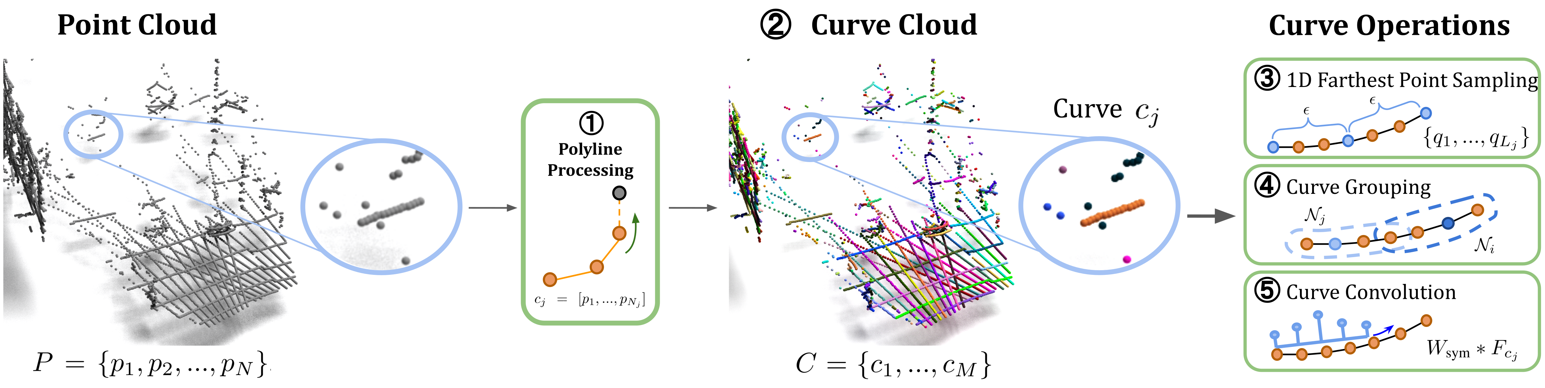
Figure 2: Overview of Curve Cloud Reasoning. Starting from laser-scanned input data, we ① link points into polylines to ② parameterize the point cloud as a curve cloud (see Sec. 3.1). We develop operations for learned architectures to specifically exploit the curve structure, including ③ 1D farthest-point-sampling along a curve, ④ curve grouping, and ⑤ symmetric curve convolutions (see Sec. 3.2).

2 Related Work

Existing point cloud methods can be roughly characterized as point-based and discretization-based approaches. As our work addresses trade-offs between them, we discuss related works from each category.

Point-Based Networks

One popular approach to point-based reasoning is to aggregate local neighborhood information in a hierarchical manner and at multiple geometric scales [40, 46, 34, 85, 47, 24, 84, 79, 45]. Recently, Ma et al. [40] introduced a modern MLP-based architecture along these lines, while Quian et al. [47] modernized the seminal PointNet++ [46] – both showed compelling results on object-level and indoor scenes. Nevertheless, most hierarchical and MLP point networks are inefficient in large-scale settings, and although several backbones [24, 84, 79] have addressed this, they trade off scalability with task-specific frameworks or lower accuracy. In contrast, CurveCloudNet scales to large scenes by using the explicit curve structure of laser scanners.

Another line of research makes use of point convolutions for learning per-point local features. Point convolutions are usually defined using kernels [51, 25, 56, 73, 16, 64, 41, 33, 28, 31, 53, 60] or graphs [52, 35, 11, 15]. Kernels have been defined using a family of polynomial functions [73], using MLPs [56, 37], or directly using local 3D point coordinates [3, 53, 64, 72, 7]. In contrast, graph methods usually construct a K-Nearest-Neighbors graph in Euclidean space [50, 55] or feature space [58], and apply graph-convolutions on the resulting edges and vertices. More recently, CurveNet [67] applied guided random walks on uniformly-sampled input point clouds to construct graph neighborhoods that go beyond K-Nearest-Neighbors and that exhibit 1D “curve” structure; then, CurveNet pooled features over the traversed curves. Aside from defining “curves”, CurveNet and CurveCloudNet have little in common: CurveNet’s guided random walks are not related to physical laser traversals and do not scale to large scenes. In contrast, CurveCloudNet efficiently recovers explicit curves from a scanner’s physical laser traversals, and then applies a variety of operations, e.g., subsampling, aggregation, and convolution, along each curve.

Many works [68, 36, 78, 82, 17, 85, 43, 65] have shown success with attention-based aggregation using transformer architectures with self-attention [54]. However, we found CurveCloudNet’s reasoning over local 1D “curve” neighborhoods to be sufficiently expressive without attention.

Discretization-Based Networks

Although point-based backbones can successfully process individual objects or small indoor scenes, they struggle to scale to large point clouds due to inefficiency in processing large unstructured point sets. To address this, several works [51, 21, 14, 38, 83, 87, 81, 76, 32, 39, 70, 23] proposed to convert a point cloud into a 3D voxel grid and use this volumetric representation. Early works converted a point cloud into a dense voxel grid and applied dense 3D convolutions [42, 44], however the cubic size of the dense grid proved to be computationally prohibitive. To scale to large scenes, several works [14, 32, 87, 39, 70, 13, 71, 74, 23, 75] employed the sparse-voxel data structure from [21]. MinkowskiNet [14] was a seminal work in showing that sparse voxel convolutions can be highly efficient and expressive. PVNAS [39] incorporated a network architecture search, demonstrating the importance of the architecture channels, network depth, kernel sizes, and training schedule. More recent works have supplemented sparse-voxel backbones with attention operations [13], range-view and point information [71], image information [75], and knowledge distillation [23].

Other methods seek a better discretization of point clouds captured with LiDAR scans. For example, PolarNet [83] proposed to partition input points using grid cells defined in a polar coordinate system, while Cylinder3D [87] employed a cylindrical partitioning scheme based on a cylindrical coordinate system. Sphereformer [30] combined polar grid cells with modern attention operations. In an alternative line of research, many methods [29, 22, 12, 2, 86, 69, 61, 64] employ spherical or bird’s-eye view projections to represent point clouds as images that are passed to a 2D convolutional or transformer network.

Unlike discretization methods, CurveCloudNet directly operates on points and curves, scaling to larger scenes without discretizing. Additionally, our curve operations are applied locally and do not assume global patterns such as polar, cylindrical, or planar structure.

3 Method: Learning on Curve Clouds

Our method takes as input a 3D point cloud, parses it into a curve cloud representation, and then processes the resulting curves by leveraging specialized curve operations, as shown in Fig. 2. We focus on object part segmentation, semantic scene segmentation, and object classification, although in principle, our method is suitable for more perception tasks.

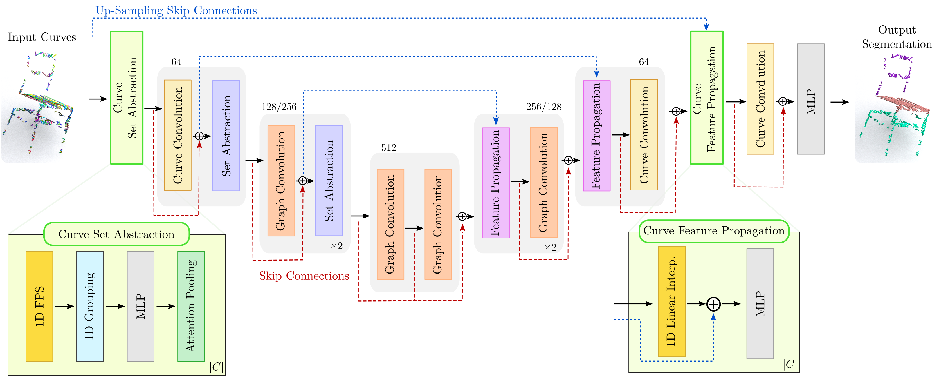
Figure 3: CurveCloudNet Architecture. The network employs a mix of curve and point layers to process a curve cloud through progressive down-sampling followed by up-sampling with skip connections. Curve layers operate on higher resolutions to efficiently capture the 1D structure, while at lower resolutions point layers propagate information across curves. Feature dimensions are listed above each block.

3.1 Constructing Curve Clouds

Problem Formulation

The input to our model is the output of a laser-based 3D sensor represented as a point cloud $P=\{p_{1},p_{2},...,p_{N}\}$, where $p_{i}=[x_{i},y_{i},z_{i}]$ is the 3D coordinates of the $i$-th point. For each point, we are also given an associated acquisition timestamp $t_{i}$ and an integer laser beam ID $b_{i}\in[1,B]$, which are readily available from sensors like LiDAR. For a scanner with $B$ unique laser beams, $b_{i}$ indicates which beam captured the point while $t_{i}$ gives the ordering in which points were captured. Timestamps differ only by microseconds and indicate point ordering for constructing the curve cloud; otherwise, the point cloud is treated as an instantaneous capture of the scene.

We assume that each laser beam in the scanner captures 3D points sequentially and at a high sampling rate as it sweeps the scene. Concretely, if points $p_{1}$, $p_{2}$, and $p_{3}$ are recorded consecutively by beam $b$, then their timestamps are ordered $t_{1}{<}t_{2}{<}t_{3}$. Moreover, if two consecutive points are spatially farther apart than some small threshold $\delta$, we assume there is a surface discontinuity and the points lie on different surfaces in the scene.

Curve Clouds

A curve $c_{j}=[p_{1},...,p_{N_{j}}]$ is defined as a sequence of $N_{j}$ points where consecutive point pairs are connected by a line segment, i.e., a polyline. The curve is bi-directional and is equivalently defined as $c_{j}=[p_{N_{j}},p_{N_{j}-1},...,p_{1}]$. A curve cloud $C=\{c_{1},...,c_{M}\}$ is an unordered set of $M$ curves where each curve may contain a different number of points. In practice, we can store a curve cloud $C$ as an $N{\times}3$ tensor of points, with an additional $ptr$ tensor of length $M$ that specifies the indices where one curve ends and the next begins. Converting the input point cloud $P$ to a corresponding curve cloud is straightforward and extremely efficient: points from each beam $b_{i}$ are ordered by timestamp and split into curves based on distances between consecutive points. If the distance between two consecutive points is more than a set threshold $\delta$ while traversing the points in time order, then the current curve ends and a new curve begins, i.e., a surface discontinuity has occurred. In practice, we parallelize this process across all points and laser beams on the GPU. More details regarding the conversion process are provided in the supplement.

Why Use Curves? Curve clouds inherit the benefits associated with the 3D point cloud representation including lightweight data structures and no need to discretize the space. But operating on curve clouds also has several advantages over point clouds. Point clouds are highly unstructured, making operations like nearest neighbor queries and convolutions expensive. Curve clouds add structure through point ordering along the polylines, allowing curves to be treated as 1D grids that permit greater cache-locality, constant-time neighborhood queries, and efficient convolutions. This structure is flexible to any laser scanning pattern unlike, e.g., cylindrical voxel grids and polar range-view projections. In principle, the curve structure should also bring out the geometric properties of the surface it represents, such as curvature, tangents, and boundaries.

3.2 Operating on Curves

We now discuss the fundamental operations for curves. We first introduce the network layers for curves followed by the details of curve operations used in these layers.

3.2.1 Curve Layers

Curve Set Abstraction (Curve SA)

Inspired by set abstraction layers from prior point-based work [46], this layer adopts a curve-centric procedure to downsample the number of points on the curves. For each curve, Curve SA (1) samples a subset of “centroid” points along the curve using our 1D farthest point sampling algorithm, (2) groups points around these centroids in local neighborhoods using curve grouping, (3) translates points into the local frame of their centroid and processes them with a shared MLP, and (4) pools over each local neighborhood to get a downsampled curve with associated point features.

Curve Feature Propagation (Curve FP)

Similar to point-based feature propagation [46], Curve FP is a curve-centric upsampling layer. For each curve $c_{j}$, this layer propagates features from the low-res polyline $[q_{1},...,q_{L_{j}}]$ with $L_{j}$ points to a higher-res polyline $[p_{1},...,p_{H_{j}}]$ with $H_{j}$ points where $L_{j}{<}H_{j}$. This is achieved using curve feature interpolation as described in Sec. 3.2.2. Afterwards, the high-res interpolated features are concatenated with skip-linked features from a corresponding curve set abstraction layer and processed by a shared MLP.

Curve Convolution

The curve convolution layer allows for efficient communication and feature extraction along a curve. This module consists of three sequential symmetric curve convolutions, each followed by batch normalization [26] and a leaky ReLU activation.

3.2.2 Curve Operations

To enable our layers to expressively and efficiently learn on curve clouds, we formulate operations for sampling, grouping, feature interpolation, and convolutions along curves.

1D Farthest Point Sampling (FPS)

FPS is frequently a bottleneck in point cloud architectures and can be costly for large point clouds [24] due to pair-wise distance computations. For curves, we alleviate this cost with an approximation of FPS along each curve independently in a 1D manner. This amounts to sampling a subset of points on each curve that are evenly-spaced along the length of that curve (i.e., geodesically). For a curve $c_{j}$ with $N_{j}$ points, we subsample points $[q_{1},...,q_{L_{j}}]$ with $L_{j}{<}N_{j}$ such that all pairs of contiguous points are about $\epsilon$ apart, where $\epsilon$ is a fixed target spacing shared across all curves. In other words, $d(q_{i},q_{i-1})\approx\epsilon$ for $i=2,\dots,L_{j}$ where $d$ measures the geodesic distance between two points along the same curve. Notably, this algorithm has only $O(N)$ complexity and can be parallelized across each curve independently.

Grouping Along Curves

After sampling, we must group points into local neighborhoods around the subsampled points on each curve. We adapt a ball query [46], which groups together all points within a specified radius from a centroid, to operate along each curve. For a centroid point $p_{i}$ belonging to curve $c_{j}$, we define the local neighborhood of $p_{i}$ as $\mathcal{N}_{i}=\{p_{k}\in c_{j}\,|\,d(p_{i},p_{k})<r\}$ where $r$ is a fixed neighborhood radius. In addition to being computationally faster than a standard 3D ball query grouping, using 1D curve groupings ensures that all neighborhoods lie on a continuous section of scanned surfaces.

Curve Feature Interpolation

To upsample on curves, we must interpolate features $[g_{1},...,g_{L_{j}}]$ from a lower-resolution polyline to features $[f_{1},...,f_{H_{j}}]$ for a higher-resolution one. Let $p_{h}$ be the h^th point on the high-res curve, which falls between subsampled low-res points $q_{i}$ and $q_{i-1}$ with associated features $g_{i}$ and $g_{i-1}$. The interpolated high-res feature $f_{h}$ is simply the distance-weighted interpolation of the two low-res point features (based on their spatial coordinates).

	ShapeNet				KortX								KortX
	Per Scan Pattern mIOU ($\uparrow$)				Per-Category IOU ($\uparrow$)								Performance
					Validation	Test
Method	Mean	Parallel	Grid	Random	mIOU	mIOU	Cap	Chair	Earphone	Knife	Mug	Rocket	Time (ms)	GPU (GB)	Param (M)
PointNet++ [46]	80.1	81.8 $\pm$ 0.1	80.1 $\pm$ 0.04	78.3 $\pm$ 0.7	66.9 $\pm$ 1.2	71.0 $\pm$ 2.5	69.3	65.9	83.1	70.4	71.7	65.5	109	1.95	1.53
DGCNN [58]	80.2	81.2 $\pm$ 0.2	80.9 $\pm$ 0.02	78.6 $\pm$ 0.3	64.6 $\pm$ 0.8	73.3 $\pm$ 0.9	73.0	76.6	81.1	79.6	58.3	71.2	143	1.45	2.18
CurveNet [67]	82.8	84.0 $\pm$ 0.2	83.8 $\pm$ 0.4	80.6 $\pm$ 0.2	68.4 $\pm$ 0.7	71.5 $\pm$ 0.4	80.9	89.7	63.6	63.0	68.0	64.0	227	1.16	5.33
PointMLP [40]	80.9	82.2 $\pm$ 0.3	81.3 $\pm$ 0.3	79.3 $\pm$ 0.3	72.1 $\pm$ 0.4	75.4 $\pm$ 1.3	77.2	75.3	78.8	83.1	64.6	73.6	58	0.83	16.76
PointNext [47]	82.8	83.8 $\pm$ 0.1	83.1 $\pm$ 0.3	81.5 $\pm$ 0.2	69.8 $\pm$ 0.6	73.7 $\pm$ 0.5	82.2	75.9	80.9	68.3	70.8	63.9	81	1.69	13.8
MinkowskiNet [14]	81.1	82.6 $\pm$ 0.3	82.0 $\pm$ 0.5	80.1 $\pm$ 0.5	62.9 $\pm$ 1.7	60.1 $\pm$ 1.4	67.5	53.2	74.3	56.4	73.6	27.5	42	0.21	36.62
Cylinder3D [87]	79.6	81.2 $\pm$ 0.1	80.1 $\pm$ 0.0	77.6 $\pm$ 0.1	58.6 $\pm$ 0.5	63.5 $\pm$ 0.2	64.8	56.9	80.8	55.1	64.8	58.7	96	5.76	56.03
SphereFormer [30]	79.5	80.3 $\pm$ 0.3	79.9 $\pm$ 0.4	78.3 $\pm$ 0.4	67.6 $\pm$ 0.9	69.7 $\pm$ 1.3	71.5	65.1	86.0	59.6	67.2	79.5	38	0.25	32.3
CurveCloudNet	83.1	83.7 $\pm$ 0.2	83.6 $\pm$ 0.5	81.9 $\pm$ 0.3	73.0 $\pm$ 0.9	78.9 $\pm$ 1.1	69.1	87.3	86.7	87.0	74.7	67.8	77	1.01	8.74

Table 2: Object Segmentation Results. Class-average mIOU is reported for synthetic ShapeNet dataset (left) and real-world Kortx data (Right). CurveCloudNet achieves the highest accuracy compared to baselines. Performance is on Nvidia RTX 3090 GPU (batch size 16).

Symmetric Curve Convolution

To process points along curves, we take advantage of expressive convolutions. However, it is computationally burdensome to compute neighborhoods on the fly and run convolutions on unordered data [39]. Instead, we treat each curve as a discrete grid of features that can be convolved similar to a 1D sequence. To account for the bi-directionality of curves, we employ a symmetric convolution and thus produce equivalent results when applied “forward” or “backward” along the curve.

In particular, for a curve $c_{j}=[p_{1},p_{2},...,p_{N_{j}}]$ with associated point features $F_{j}=[f_{1},f_{2},...,f_{N_{j}}]$, we start by extracting additional features using the the L1 norm of feature gradients along the curve [60], denoted as $\nabla F_{j}=\big{[}|\nabla f_{1}|,|\nabla f_{2}|,...,|\nabla f_{N_{j}}|\big{]}$. Note the norm is necessary to remove directional information. Concatenating these features together as $[F_{j},\nabla F_{j}]\in\mathbb{R}^{N_{j}\times D}$ gives a grid on which to perform 1D convolutions. To respect bi-directionality, symmetric kernels are used for the convolution: for a kernel $W\in\mathbb{R}^{S\times D}$ with size $S$ and $D$ channels, we ensure $W_{i}=W_{S-i+1}$ for $i=1,\dots,S$ where $W_{i}\in\mathbb{R}^{D}$.

3.3 Curve Cloud Backbone: CurveCloudNet

In Fig. 3, we illustrate CurveCloudNet as designed for segmentation tasks where the output is a single semantic class (one-hot vector) for each point in the input point cloud. Hence, it follows the U-Net [49] structure, consisting of a series of downsampling layers followed by upsampling with skip connections. Although in our experiments (Sec. 4) we focus on segmentation, CurveCloudNet can be adapted to other point cloud perception tasks (see supplement for a classification example).

Our architecture is a mix of curve and point-based layers. At higher resolutions, curve modules are employed since they are efficient and can capture geometric details when curve sampling is most dense across surfaces in the scene. At lower resolutions, point modules are used to propagate information across curves when 1D structure is less apparent. For point operations, we adopt the set abstraction and feature propagation operations from [46] as well as the graph convolution from [58], and we further improve these point operations following the reportings of recent works [24, 40, 47] (see supplementary for further details). By combining curve and point operations, CurveCloudNet is an expressive network that maintains the benefits of point cloud backbones while injecting structure and efficiency previously only possible with voxel-based approaches.

4 Experiments

We evaluate CurveCloudNet and a set of competitive baselines on five datasets – the ShapeNet Part Segmentation dataset [10], the KortX Part Segmentation dataset, the Audi Autonomous Driving Dataset (A2D2) [20], the nuScenes dataset [8], and the Semantic KITTI dataset  [4, 19]. Each dataset exhibits a unique structure and training setup (see  Tab. 1b). Put together, our evaluation consists of indoor, outdoor, object-centric, scene-centric, sparsely scanned, and densely scanned scenes. Furthermore, each of the five datasets display different point sampling patterns, which we roughly characterize as following “parallel”, “grid”, or “random” laser motions (see  Fig. 1).

CurveCloudNet achieves the best or second best performance on all datasets, and on average outperforms all previous methods (see Tab. 1a). Furthermore, every other method substantially underperforms CurveCloudNet on at least one dataset. Notably, CurveCloudNet outperforms point-based backbones on object-level tasks and is competitive with or better than voxel-based backbones on larger scenes. In Sec. 4.1 we evaluate our model on the task of object-level part segmentation on simulated ShapeNet [10] objects and on a new dataset collected with the Kortx vision system [1]. In Sec. 4.2, Sec. 4.3, and Sec. 4.4, we evaluate semantic segmentation on larger outdoor scenes using the Audi Autonomous Driving Dataset (A2D2) [20], the nuScenes dataset [8], and the Semantic KITTI dataset [4, 19]. Sec. 4.5 ablates the key components of CurveCloudNet. In the supplementary, we report additional qualitative results and an experiment on object classification.

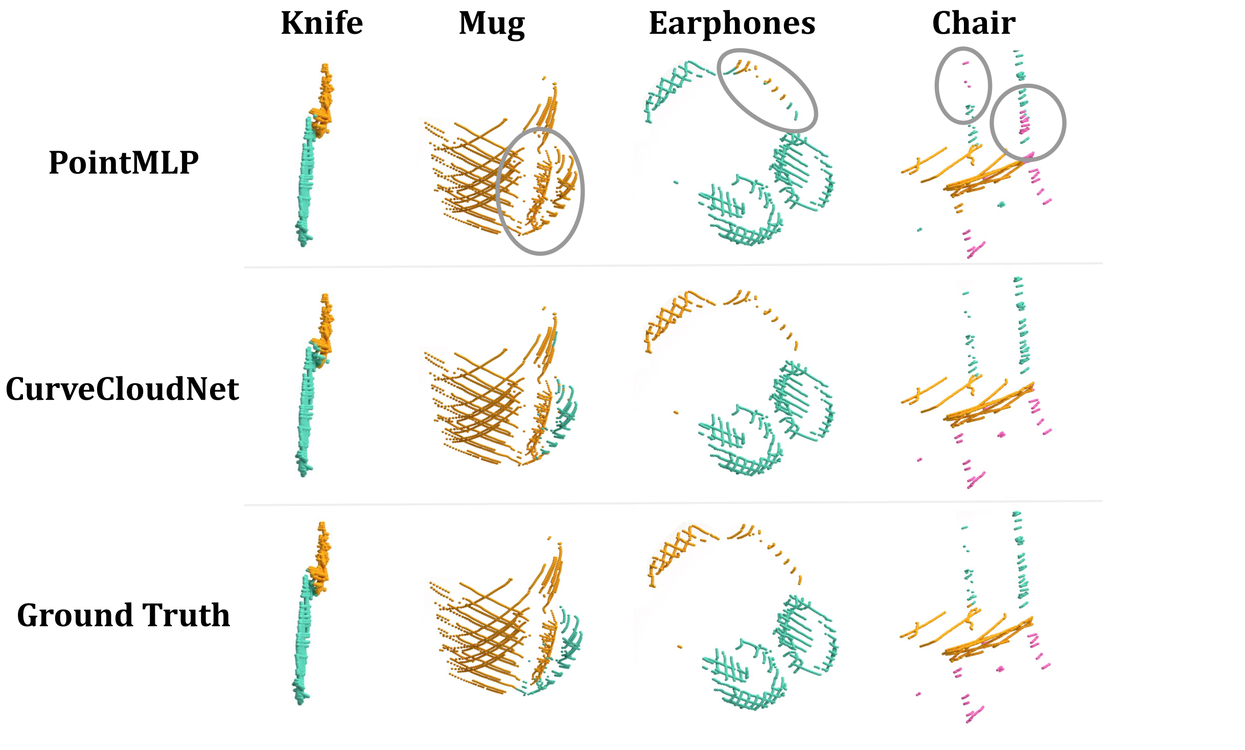
Figure 4: Qualitative Results on Kortx. CurveCloudNet successfully segments fine-grained parts by leveraging curve structures.

			Performance ($\downarrow$)			Per-Class mIoU ($\uparrow$)
Method	Type	mIoU ($\uparrow$)	Time (ms)	GPU (GB)	Param (M)	car	bicycle	truck	person	road	sidewalk	obstacle	building	nature	pole	sign	signal
PointNet++ [46]	Point	46.5	53	0.19	1.52	62.4	9.3	55.7	3.6	90.3	58.0	12.7	79.3	82.1	19.2	36.6	48.7
RandLANet [24]		43.4	16	0.05	1.24	60.2	4.8	46.7	7.5	91.3	57.2	14.9	78.9	80.0	16.6	27.7	34.3
CurveNet* [67]		4.4	385	1.77	5.52	0.0	0.0	0.0	0.0	25.4	0.0	0.0	0.0	26.9	0.0	0.0	0.0
PointMLP [40]		47.6	63	0.86	16.8	65.8	9.8	54.2	15.8	92.5	63.5	14.8	81.7	82.9	18.8	34.6	36.9
PointNext [47]		45.0	34	0.33	41.6	62.6	2.6	63.1	1.0	91.1	58.7	12.8	80.1	81.8	12.5	33.8	39.3
MinkowskiNet [14]	Voxel	53.8	37	0.19	36.6	70.3	13.7	77.6	26.8	92.8	67.5	18.0	80.8	81.9	18.0	40.5	58.1
Cylinder3D [87]		53.0	61	1.18	55.8	71.1	11.6	74.8	22.1	92.5	66.1	18.3	82.6	84.2	19.1	41.6	52.0
SphereFormer [30]		55.1	54	0.37	32.3	76.3	11.5	68.9	26.0	93.8	70.1	19.6	84.0	86.6	19.8	46.2	58.9
CurveCloudNet	Curve	54.1	75	0.27	10.2	71.9	12.9	78.6	22.3	93.2	68.5	19.8	83.3	85.6	17.4	44.3	51.4

Table 3: A2D2 Segmentation Results. On grid-like LiDAR scans, CurveCloudNet outperforms all point-based backbones in mIoU and is competitive with SphereFormer. Performance is on an Nvidia RTX 3090 GPU (batch size 1).

4.1 Object Part Segmentation

ShapeNet Dataset

The ShapeNet Part Segmentation Benchmark [9, 80] contains 16,881 synthetic shape models across 16 different categories and 50 object parts. To evaluate performance on the laser-based scans that we are interested in, we simulate laser capture using the ShapeNet meshes. Using a fixed front-facing sensor pose, we raycast a set of linear laser traversals and then sample points on the mesh along each traversal. We consider three types of synthetic laser traversals - parallel, grid, and random - which are depicted on the left side of Fig. 1 and are further described in the supplementary. We generate one synthetic scan for each ShapeNet mesh, which yields 12139 training point clouds and 1872 validation point clouds.

ShapeNet Results

ShapeNet results are summarized on the left side of Tab. 2. All methods are trained over three random seeds, and we report the mean and standard deviation of the class-averaged mean intersection-over-union (mIOU) over the runs. For fair comparison, all models are trained for 120 epochs using the same hyperparameters, and the best validation mIOU throughout training is reported.

On average, CurveCloudNet outperforms all baselines and performs disproportionately well for the “random” laser traversals. In contrast, SphereFormer exhibits the lowest accuracy of all methods, suggesting that its radial window attention is poorly suited for individual objects. CurveNet and PointNext are the runner ups, showing strong performance on segmenting objects when the scans are captured from the front-facing sensor pose.

Kortx Dataset

Kortx is a perception software system developed by Summer Robotics [1] that generates and operates on 3D curves sampled from a triangulated system of event sensors and laser scanners. Kortx software supports arbitrary continuous scan patterns, and in practice we scan objects with a randomly shifted Lissajous trajectory per laser beam. Using Kortx, we scan $7$ real-world objects (cap, chair, earphone, knife, mug-1, mug-2, and rocket) multiple times in different poses, collecting 195 point clouds in total. We will release this dataset upon publication. We train on scans that are simulated from ShapeNet meshes and evaluate on the Kortx scans as well as the ShapeNet validation split. To best mimic the Kortx data, we simulate random laser traversals on each ShapeNet mesh and only train on the six object categories present in the Kortx dataset: cap, chair, earphone, knife, mug. We generate five training scans per ShapeNet object, each scanned from a unique random sensor pose. This yields a training set of 31,991 point clouds.

KortX Results

KortX results are summarized on the right side of Tab. 2. The experimental setup is identical to ShapeNet, except we train over four random seeds and for 60 epochs. CurveCloudNet again outperforms all baselines, showing effective generalization to out-of-domain Kortx test scans. Voxel-based methods continue to underperform their point-based counterparts, suggesting that discretizing the input has a negative effect when point clouds are small. In contrast to the previous ShapeNet evaluation, PointMLP is the second-best method when scans are captured from random sensor poses. Fig. 4 shows that CurveCloudNet better distinguishes fine-grained structures, such as the back of a chair, a mug handle, and an earphone headpiece.

			Performance ($\downarrow$)			Per-Class mIoU ($\uparrow$)
Method	Type	mIoU ($\uparrow$)	Time (ms)	GPU (GB)	Param (M)	barrier	bicycle	bus	car	construction	motorcycle	pedestrian	traffic cone	trailer	truck	driveable	other flat	sidewalk	terrain	manmade	vegetation
PointNet++ [46]	Point	51.1	274	0.60	1.5	60.1	6.5	58.4	66.3	16.4	20.0	50.8	12.6	31.5	42.0	94.0	60.8	63.8	69.2	82.4	82.3
RandLANet [24]		62.9	21	0.18	1.2	72.5	12.6	36.6	81.8	38.7	72.3	68.5	37.3	44.7	59.7	95.3	87.0	69.7	71.1	73.2	85.9
CurveNet [67]		–	–	$>$48	5.5	–	–	–	–	–	–	–	–	–	–	–	–	–	–	–	–
PointMLP [40]		67.9	164	4.94	16.8	72.3	27.8	88.2	86.3	37.2	51.0	60.7	50.6	56.4	71.1	95.7	70.6	70.9	72.0	88.8	87.2
PointNext [47]		65.0	155	0.62	41.5	68.7	1.2	86.9	87.5	41.8	57.4	54.3	34.9	55.3	75.1	95.7	68.9	70.2	71.5	86.5	84.0
MinkowskiNet [14]	Voxel	76.2	44	0.29	36.6	75.4	43.9	91.9	93.0	49.0	84.3	78.3	64.6	65.9	85.7	96.1	71.5	67.5	74.8	86.5	84.9
PolarNet* [83]		71.0	-	-	-	74.7	28.2	85.3	90.9	35.1	77.5	71.3	58.8	57.4	76.1	96.5	71.1	74.7	74.0	87.3	85.7
Cylinder3D* [87]		76.1	80	1.57	55.9	76.4	40.3	91.2	93.8	51.3	78.0	78.9	64.9	62.1	84.4	96.8	71.6	76.4	75.4	90.5	87.4
SphereFormer* [30]		79.5	59	0.81	32.3	78.7	46.7	95.2	93.7	54.0	88.9	81.1	68.0	74.2	86.2	97.2	74.3	76.3	75.8	91.4	89.7
CurveCloudNet	Curve	78.0	87	1.14	28.8	77.3	45.7	92.4	91.9	59.4	84.5	78.5	64.1	69.6	85.0	96.9	72.7	75.6	75.2	90.5	89.0

Table 4: nuScenes Segmentation Results. On typical sweeping LiDAR scans, CurveCloudNet scales significantly better than other point-based backbones and is competitive with recent work SphereFormer. Performance is on an Nvidia RTX 3090 GPU (batch size 1). * indicates that results are copied from the referenced papers.

4.2 A2D2 LiDAR Segmentation

A2D2 Dataset

The Audi Autonomous Driving Dataset (A2D2) [20] contains 41,280 frames of outdoor driving scenes captured from 5 overlapping LiDAR sensors, creating a unique grid-like scanning pattern (see Fig. 2). Each frame is annotated from the front-facing camera with a 38-category semantic label. We define a mapping from camera categories to LiDAR categories and remove texture-only (e.g. sky, lane markers, blurred-area) and very rare categories (e.g. animals, tractors, utility vehicles). In total, we evaluate on 12 LiDAR categories: car, bicycle, truck, person, road, sidewalk, obstacle, building, nature, pole, sign, and traffic signal. Evaluation is performed on annotated LiDAR points in the field of view of the front-facing camera.

Results

We train CurveCloudNet along with point and voxel-based baselines on the official A2D2 training split [20]. For fair comparison, all models are trained for 140 epochs using the same hyperparameters, and the best validation mIOU throughout training is reported. Results are summarized in Tab. 3, and Fig. 1 provides a qualitative example. CurveCloudNet scales to outdoor scenes better than point-based backbones, with the runner-up PointMLP showing a 6% drop in mIOU. CurveCloudNet also outperforms most voxel-based backbones and achieves similar accuracy to state-of-the-art SphereFormer [30], even though SphereFormer’s radial window attention is tailored for outdoor LiDAR scans.

4.3 nuScenes LiDAR Segmentation

nuScenes Dataset

The nuScenes dataset [8] contains 1000 sequences of driving data, each 20 seconds long. Each sequence contains 32-beam LiDAR data with segmentations annotated at 2Hz. We follow the official nuScenes benchmark protocol with 16 semantic categories.

Results

We train CurveCloudNet and baselines on the official nuScenes training split. To ensure fair comparison, we train all models for 100 epochs. Results on the nuScenes validation split are shown in Tab. 4, and Fig. 1 includes a qualitative example. CurveCloudNet significantly improves upon other point-based networks: PointMLP and PointNext show more than a 10% drop in mIOU and $\sim 2\times$ increase in latency. We also note that CurveNet exceeds 48GB of GPU memory for a batch size of 1, showcasing its inability to scale to larger scenes. CurveCloudNet also outperforms all voxel-based methods except the recent SphereFormer.

4.4 KITTI LiDAR Segmentation

The Semantic KITTI dataset is made up of 22 sequences of driving data consisting of 23,201 LiDAR scans for training and 20,351 for testing. Each scan is obtained with a dense 64-beam Velodyne LiDAR. We follow the official KITTI protocol in training and validation. To ensure fair comparison, we train all models for 100 epochs. Results on the validation sequence are reported in Tab. 5, and Fig. 1 shows a qualitative example. CurveCloudNet outperforms all point-based and voxel-based methods. Note that we cannot report results for many point-based methods due to excessive training times on the larger KITTI scans ($>20$ days).

			Performance ($\downarrow$)
Method	Type	mIoU ($\uparrow$)	Time (ms)	GPU (GB)	Param (M)
PointNet++ [46]	Point	–	2690	11.1	1.6
CurveNet [67]		–	–	$>$48	5.5
PointMLP [40]		39.5	293	5.24	16.8
PointNext [47]		–	1303	1.83	41.6
MinkowskiNet [14]	Voxel	66.8	111	0.53	36.6
Cylinder3D* [87]		68.9	233	1.62	55.9
SphereFormer* [30]		69.0	144	3.46	32.3
CurveCloudNet	Curve	69.5	155	2.75	28.8

Table 5: Quantitative results on the KITTI validation split. Performance is on an Nvidia RTX 3090 GPU (batch size 1). * indicates results are copied from the referenced papers.

4.5 Ablation Study

Curve Operations				Performance ($\downarrow$)
Grouping	FPS	1D Conv.	mIoU ($\uparrow$)	Time (ms)	GPU (GB)	Param (M)
✓	✓	✓	54.1	75	0.27	10.3
✗	✓	✓	53.3	99	1.03	10.3
✓	✗	✓	52.4	105	0.26	10.3
✓	✓	✗	52.0	61	0.20	9.9
✗	✗	✗	52.6	122	0.92	10.3

Table 6: Ablation Study on A2D2. Curve operations are ablated and replaced with the standard point-based counterparts.

Tab. 6 shows an ablation analysis of CurveCloudNet on the A2D2 dataset; the table shows that each of our proposed curve operations is essential to achieve high accuracy and efficiency. We ablate grouping along curves by instead using the regular radial groupings from PointNet++ [46]. This ignores the curve structure and results in decreased accuracy, increased latency, and a significant increase in GPU memory usage. Instead of curve farthest point sampling, we also try regular FPS, which causes a decreased accuracy and increased latency. Finally, without 1D curve convolutions, we observe a notable decline in accuracy with a marginal improvement in latency and GPU memory. Taken together, our curve operations increase accuracy with roughly half the latency and one third the GPU memory requirements.

5 Discussion and Limitations

We have described a point cloud processing scheme and backbone, CurveCloudNet, which introduces curve-level operations to achieve accurate, efficient, and flexible performance on point cloud segmentation. CurveCloudNet outperforms or is competitive with previous methods on the ShapeNet, Kortx, A2D2, nuScenes, and KITTI datasets, and on average achieves the best performance. Put together, CurveCloudNet is a unified solution to both small and large-scale scenes with various scanning patterns.

Nevertheless, CurveCloudNet has limitations. First, CurveCloudNet is only designed for laser-scanned data, i.e. point clouds with explicit curve structure due to 1D laser traversals. We believe a promising future direction is to investigate virtual curves that could extend CurveCloudNet to uniformly sampled point clouds. Furthermore, we believe that future research can continue to improve curve operations. While our proposed curve operations yield significant improvements, an exciting future direction will be to investigate explicit curve-to-curve communication, curve self-attention and cross-attention, and curve intersections.

S 1 Overview

In this document, we provide additional method details, dataset details, implementation details, experimental analysis, and qualitative results. In Sec. S 2, we concretely outline how we convert a point cloud into a curve cloud and how we implement our 1D farthest point sampling algorithm. In Sec. S 3, we provide a detailed overview of the Kortx software system and dataset, our ShapeNet simulator, and the A2D2 dataset. In Sec. S 4, we discuss implementation details of CurveCloudNet not covered in the main paper. Finally, in Sec. S 5, we report results covering GPU memory analysis, object classification, ShapeNet segmentation, and the nuScenes test split.

S 2 Additional Method Details

S 2.1 Constructing Curve Clouds

Curve Cloud Conversion

⬇

”’

Inputs:␣P,␣T,␣B,␣delta

␣␣␣␣P:␣array␣of␣size␣(N,␣3)␣with␣xyz␣coordinates

␣␣␣␣T:␣array␣of␣size␣(N,)␣with␣timesteps

␣␣␣␣B:␣array␣of␣size␣(N,)␣with␣beam␣IDs

Outputs:␣curves

␣␣␣␣curves:␣list␣of␣arrays,␣array␣j␣is␣size␣(N_j,␣3)

’”

curves = []

for b in unique(B):

# filter to a single laser beam’s measurments

beam_P, beam_T = P[beams==b], T[beams==b]

# order points by laser’s traversal

sequential_ordering = argsort(beam_T)

beam_P = beam_P[sequential_ordering]

# split laser’s traversal into cont. curves

edge_lens = norm(beam_P[1:] - beam_P[:-1])

split_locations = edge_lens > delta

# convert into polylines

beam_C = split_seq(beam_P, split_locations)

curves += beam_C

Figure S1: Point to Curve Cloud Conversion. Algorithm (in Python) to convert an input point cloud into a set of polylines.

Constructing Curve Cloud

We refer the reader to Sec. 3.1 of the main paper for an overview of constructing curve clouds. As input, we assume that a laser-based 3D sensor outputs a point cloud $P=\{p_{1},...,p_{N}\}$ where $p_{i}=[x_{i},y_{i},z_{i}]\in\mathbb{R}^{3}$, an acquisition timestamp $t_{i}\in\mathbb{R}$ for each point, and an integer laser-beam ID $b_{i}\in[1,B]$ for each point. We wish to convert the input into a curve cloud $C=\{c_{1},...,c_{M}\}$, where a curve $c=[p_{i},...,p_{i+K}]$ is defined as a sequence of $K$ points where consecutive point pairs are connected by a line segment, i.e., a polyline. As outlined in Fig. S1, we first group points by their laser beam ID and sort points based on their acquisition timesteps, resulting in an ordered sequence of points that reflects a single beam’s traversal through the scene. Next, for each sequence, we compute the distances between pairs of consecutive points (denoted as polyline “edge lengths”). Finally, we split the sequence whenever an edge length is greater than a threshold $\delta$, resulting in many variable-length polyline “curves”. In practice, we parallelize the conversion across all points, and on the large-scale nuScenes dataset, the algorithm runs at 1500Hz.

We select a threshold $\delta$ that reflects the sensor specifications and scanning environment. In particular, the threshold is conservatively set to approximately $10\times$ the median distance between consecutively scanned points one meter away from the sensor. On the A2D2 dataset [20], we set $\delta=[0.1,0.17,0.1,0.12,0.1]$ for the five LiDARs, and on the nuScenes dataset [8] and KITTI dataset [4, 19] we set $\delta=0.08$. Additionally, on the A2D2, nuScenes, and KITTI datasets, we scale $\delta$ proportional to the square root of the distance from the sensor, since point samples becomes sparser at greater distance. On the object-level ShapeNet dataset [9], we set $\delta=0.01$. Experimentally, we observed that CurveCloudNet is flexible across different $\delta$ values.

Kortx Curve Representation

The Kortx vision system directly generates and operates on 3D curves sampled from a triangulated system of event-based sensors and laser scanners. As the detected laser reflection traverses the scene, it produces a frameless 4D data stream that enables low latency, low processing requirements, and high angular resolution. 3D curves are an intrinsic component of the Kortx perception system, and the system directly outputs a curve cloud without the need for additional data processing.

S 2.2 Additional Details on Curve Operations

1D Farthest Point Sampling

We refer the reader to Sec. 3.2.2 of the main paper for an overview of our 1D farthest point sampling (FPS) algorithm. The goal of this algorithm is to efficiently sample a subset of points on each curve such that consecutive points will be approximately $\epsilon$ apart along the downsampled curve. Concretely, for a curve $c$ with $K$ points, $c=[p_{i},...,p_{i+K}]$, we first compute the $K{-}1$ “edge lengths”, $e=[d_{i},...,d_{i+K-1}]$, where $d_{i}$ is the distance between consecutive points $(p_{i},p_{i+1})$. Next, we estimate the geodesic distance along the curve via a cumulative sum operation on the edge lengths: $g=\texttt{CUMSUM}(e)$. Then, we divide the geodesic distances by our desired spacing, $\epsilon$, and take the floor, resulting in $\epsilon$-spaced intervals $I=\texttt{FLOOR}(g/\epsilon)$. We output the first point in each interval, resulting in $L$ $\epsilon$-spaced subsampled points $\{q_{1},...,q_{L}\}$.

For each curve, the computational complexity of the 1D FPS algorithm is $O(K)$. Extending this to all curves, the computational complexity is $O(N)$. When parallelized on a GPU, for each curve, the 1D FPS algorithm has a has parallel complexity of $O(\log K)$, where the CUMSUM operation is the parallelization bottleneck (see prefix sum algorithms for more information [6]). The algorithm trivially parallelizes across curves, leading to a total parallel complexity of $O(\log K)$. In contrast, Euclidean farthest point sampling has a comptational complexity of $O(N^{2})$ or $O(Nlog^{2}N)$ (depending on whether a KD-tree is used), and a parallel complexity of $O(L)$. When $L$ is large (i.e. we are subsampling a large number of points), Euclidean FPS is a significant performance bottleneck.

S 2.3 Additional Details on Point Operations

Set Abstraction (SA)

CurveCloudNet uses a series of set abstraction layers from PointNet++ [46], and we follow previous works to improve the set abstraction layer. First, we perform relative position normalization [47] – given a centroid point $p_{i}$ with local neighborhood points $\mathcal{N}_{i}$, we center the neighborhood about $p_{i}$ and we divide by $r$ to normalize the relative positions. Additionally, we opt for the attentive pooling from RandLANet [24] instead of max pooling.

Graph Convolution

CurveCloudNet uses a series of graph convolutions, which are modeled after the edge convolution from DGCNN [58]. Unlike DGCNN however, we construct the K-Nearest-Neighbor graph based on 3D point distances instead of feature distances – this permits more efficient neighborhood construction, irrespective of feature size. Furthermore, we use attentive pooling from RandLANet [24] instead of max pooling.

S 3 Additional Dataset Details

S 3.1 Kortx Perception System and Dataset

Kortx Perception System

Kortx is a perception software system developed by Summer Robotics [1]. It is an active-light, multi-view stereoscopic system using one or more scanning lasers. It can be configured to use two or more event-based vision sensors to build up arbitrary capture volumes. Event-based vision sensors are used to detect the scanning laser reflection from target surfaces. Event-based sensors are well suited to this setup as their readout electronics are event triggered instead of time triggered. Furthermore, the Kortx System supports arbitrary continuous scan patterns, allowing a user to create their own patterns and use their own scan hardware. For more information, please visit the Summer Robotics Website.

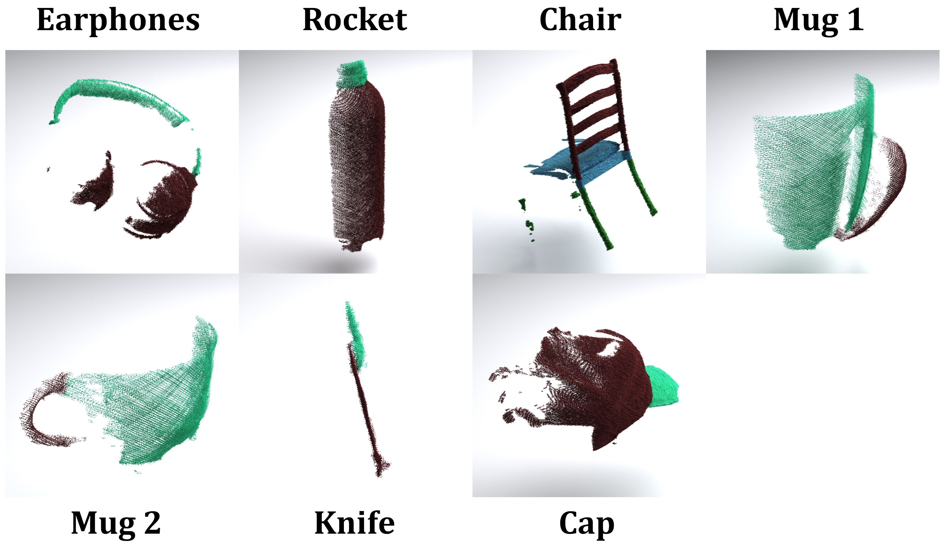
Figure S2: Kortx Dataset Objects. Our Kortx dataset contains scans of 7 real-world objects. We visualize one aggregated “scan” per object from a single viewpoint.

Object	Total	Cap	Chair	Earphone	Knife	Mug	Rocket
Instances	7	1	1	1	1	2	1
Scans	39	6	6	4	6	12	5
Frames	195	30	30	20	30	60	25

Table S1: Kortx Dataset Statistics. “Instance” is a unique 3D object. “Scan” is a dense object scan from a single viewpoint. “Frame” is a single frame within the 20Hz stream of the dense scan.

Kortx Dataset

Using Kortx, we scanned $7$ real-world objects: cap, chair, earphone, knife, mug-1, mug-2 and rocket (see Fig. S2). Each object was scanned multiple times in different poses, resulting in $39$ total scans (summarized in Tab. S1). Because the Kortx platform provides a continuous event-based 3D scan output (points are sampled every 5µs), we defined a “frame” as a batch of 2048 consecutive point measurements, corresponding to roughly a 20Hz frame rate. Because each frame differs in its dynamic scanning pattern, we evaluate on 5 consecutive frames per scan in our Kortx dataset, hence resulting in 195 point clouds in total. We manually labeled scanned points with the semantic part categories defined in the ShapeNet Part Segmentation Benchmark [9]. Each Kortx scan is mean-centered, however it is not aligned into a canonical pose, resulting in an object’s orientation depending on the sensor’s reference frame.

S 3.2 ShapeNet Simulator

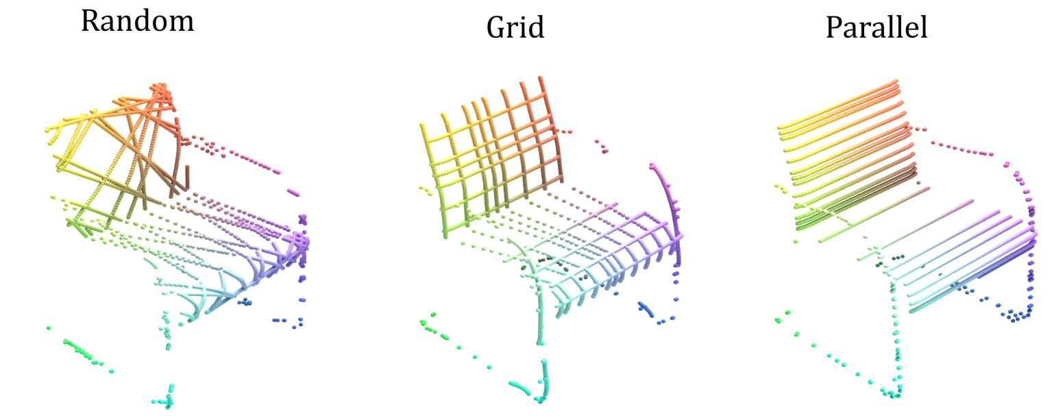
Figure S3: ShapeNet Simulator. Our ShapeNet laser-based 3D capture simulator can produce different types of sampling patterns.

We simulate laser-based 3D capture on the ShapeNet Dataset [9]. For each mesh, we randomly sample a sensor pose on the unit sphere and render the mesh’s depth values into a $2048\times 2048$ image. Next, we sample 2D lines on the depth image that correspond to a laser’s traversal. For the random sampling pattern used in the Kortx evaluation (see Sec 4.1 of the main paper) and the ShapeNet Classification evaluation (see Sec. S 5.2), we select random linear traversals in the image plane, with each traversal parameterized by a pixel coordinate $(i,j)$ and direction $\theta\in[0,\pi)$. For the grid and parallel sampling patterns used in our ShapeNet Segmentation evaluation (see Sec 4.1 of the main paper), we sample evenly-spaced vertical and horizontal lines. To reduce descritization artifacts introduced from the rasterization, we query every 6th pixel along each line for the Kortx segmentation task and every 4th pixel for the ShapeNet segmentation and classification tasks. We repeatedly generate synthetic laser traversals until we have sampled 2048 points from the mesh. Fig. 1 of the main paper shows an example of the random, grid, and parallel sampling patterns used in our ShapeNet Segmentation evaluation. Fig. S3 provides an additional qualitative illustration of the three sampling patterns, but showing 4096 points per scan for greater visual clarity.

S 3.3 A2D2 LiDAR Segmentation

The Audi Autonomous Driving Dataset (A2D2) [20] contains 41,280 frames of labeled outdoor driving scenes captured in three cities. The vehicle is equipped with five LiDAR sensors, each mounted on a different part of the vehicle and with a different orientation, resulting in a unique grid-like scanning pattern. The A2D2 data was captured in urban, highway, and rural environments as well as in different weather conditions. At the time of writing, the A2D2 dataset only contains semantic labels for the front-facing camera. Thus, we evaluate on LiDAR observations within the front-facing camera’s field of view, and we map camera categories to LiDAR categories. We will release the code detailing the exact mapping.

S 3.4 Discussion on 3D Datasets

As LiDAR and other 3D scanning technologies continue to develop, they are being applied to new and diverse applications, including open-world robotics (i.e. embedded agents), city planning, agriculture, mining, and more. Additionally, there is an increasing variety of sensors and sensor configurations, spanning hardware that scans at different point densities, different ranges, and with unique (or controllable) scanning patterns. The A2D2 and Kortx datasets are two recent examples of such a trend. We believe an important future direction will be to develop a 3D backbone that is performant in all these settings. Furthermore, we believe it is important to understand which settings “break” previous assumptions such as the range-view projection, the birds-eye-view projection, and spherical attention. While CurveCloudNet is a first step towards this goal, we believe it will be important to capture and compile new 3D datasets, and to evaluate on a greater diversity of environments.

S 4 Additional Implementation Details

S 4.1 Baselines

PointNet++ and DGCNN

We train and evaluate PointNet++ [46] and DGCNN [59] using the reproduced implemenations from Pytorch Geometric [18]. For PointNet++, we run hyperparameter sweeps to tune the radius and downsampling ratio on each dataset. For DGCNN, we use the authors’ reported hyperparameters.

RandLANet

We train and evaluate RandLANet [24] using the reproduced implementation from Open3D-ML [88]. We additionally improve the latency by incorporating GPU-implementations for point grouping and sampling from PyTorch3D [48]. We use the authors’ reported hyperparameters.

CurveNet

We train and evaluate CurveNet [67] using the authors’ official implementation. We use the authors’ reported hyperparameters for all datasets.

PointMLP

We train and evaluate PointMLP [40] using the authors’ official implementation. We use the reported hyperparameters for all datasets.

PointNext

We train and evaluate PointNext [47] using the authors’ official implementation. As outlined by the authors, we use PointNext-Small for the ShapeNet and KortX datasets. On the A2D2, nuScenes, and KITTI datasets, we use the larger PointNext-XL. Because the authors indicate the importance of the network “radius”, we additionally performed a hyperparameter sweep to find the best radius of 0.05 for the A2D2, nuScenes, and KITTI datasets.

MinkowskiNet

We train and evaluate MinkowskiNet [14] using the authors’ official implementation. We use the larger MinkUNet-34A for all experiments. We use an initial voxel size of $0.05$ on outdoor datasets and $0.015$ on object-level datasets.

Cylinder3D

We train and evaluate Cylinder3D [87] using the authors’ official implementation. We use the reported hyperparameters on the nuScenes and KITTI datasets. On the A2D2 dataset, we set the cylindrical voxel grid to cover a $\pm 31^{\circ}$ forward-facing azimuth with a maximum radius of 80 meters and a height covering $[-5,20]$ meters; we define the initial grid to have 360 radial partitions, 120 angular partitions, and 120 height partitions. On the ShapeNet and KortX datasets, we set the voxel grid to cover all $360^{\circ}$ with a radius of $1.0$ and height of $1.0$; to address latency and memory constraints, we define the initial grid to have 96 radial partitions, 96 angular partitions, and 96 height partitions.

SphereFormer

We train and evaluate SphereFormer [30] using the authors’ official implementation. We use the reported hyperparameters for the nuScenes and KITTI datasets, and we use the reported nuScenes hyperparameters for the A2D2 dataset. For the KortX and ShapeNet datasets, we also use the reported hyperparameters, and we reduce the voxel size from $0.1$ to $0.015$ to account for the dataset’s smaller 3D scale. On the KortX and ShapeNet datasets, we additionally ran a sweep on different voxel sizes and spherical window sizes, but observed limited differences.

S 4.2 Training Strategy

We train CurveCloudNet and baselines on segmentation tasks with a standard cross-entropy loss. Following previous works, we also supplement the loss with a Lovasz loss [5, 87] for the nuScenes, A2D2, and KITTI datasets. At training, we apply random scaling and translation augmentations, as well as random flips on the nuScenes, A2D2, and KITTI datasets. Importantly, we use an identical training strategy for CurveCloudNet and each baseline. We experimentally observe convergence in all models’ validation accuracies by the end of training.

Object Part Segmentation

We train CurveCloudNet and all baselines for 60 epochs in the KortX experiment and 120 epochs in the ShapeNet experiment with the Adam optimizer [27], a learning rate of $1e^{-4}$, batch momentum decay of $0.97$, and exponential learning rate decay of $0.97$. For all models, except for Cylinder3D, we use a batch size of 24. For Cylinder3D, we use a batch size of 12 because 24 exceeds our GPU memory capacity.

A2D2 LiDAR Segmentation

We train CurveCloudNet and all baselines for 140 epochs with the Adam optimizer, a batch size of 7, a learning rate of $1e^{-3}$, and an exponential learning rate decay of $0.97$.

nuScenes and KITTI LiDAR Segmentation

We train CurveCloudNet and all baselines for 100 epochs with the Adam optimizer, a batch size of 4 on nuScenes and 2 on KITTI, a learning rate of $1e^{-3}$, and an exponential learning rate decay of $0.97$. At test time, we follow previous works [87, 39] and average model predictions over axis-flipping and scaling augmentations.

S 5 Additional Experiments

		Per-Class mIoU ($\uparrow$)
Method	mIoU ($\uparrow$)	car	bicycle	truck	person	road	sidewalk	obstacle	building	nature	pole	sign	signal
MinkowskiNet [14]	42.7	54.7	3.1	60.0	7.4	87.3	54.8	9.7	71.8	76.7	14.3	31.5	42.4
SphereFormer [30]	40.5	52.7	1.1	62.4	3.8	85.9	53.5	10.9	70.5	76.3	9.6	29.1	29.9
CurveCloudNet	44.8	58.4	2.2	59.8	6.7	89.9	58.5	11.1	77.8	83.3	13.1	35.6	42.2

Table S2: Translated A2D2 Results. When A2D2 scans are randomly translated, CurveCloudNet significantly outperforms SphereFormer, suggesting that SphereFormer relies on a dataset exhibiting a highly consistent global structure.

S 5.1 Translated A2D2

Overview

In Sec. 4.2 of the main paper, we reported that SphereFormer outperforms CurveCloudNet by $+1.0\%$ mIOU on the A2D2 dataset. In this section, we show that, on the same data, SphereFormer underperforms CurveCloudNet when the scene does not exhibit consistent and aligned global structure.

We apply a simple translation augmentation to the A2D2 training and validation data – for each scan, we offset all points by a translation sampled from a uniform Gaussian with $\mu=0$ and $\sigma=20$. Note that this removes the global alignment of point clouds, but completely preserves all local structure. In the real world, this setup could occur in topography or mapping, i.e. when a large region is scanned but only one area is of interest (which could be anywhere in the scan). We train and evaluate all models with an identical setup to the original A2D2 experiment.

Results

We summarize results on the translated A2D2 experiment in Tab. S2. Without a consistent global alignment of the scene layout, all methods perform worse. However, CurveCloudNet is less effected and outperforms SphereFormer by over 4$\%$. This further suggests that SphereFormer’s radial window is tailored for outdoor driving scenes and cannot be flexibly applied to environments with weaker global structure. In contrast, CurveCloudNet can successfully leverage local structures to reason in more diverse environments.

	Accuracy			Performance
Method	Class ($\uparrow$)	Instance ($\uparrow$)	F1 ($\uparrow$)	Time (ms) ($\downarrow$)	GPU (GB) ($\downarrow$)	Param (M)
PointNet++ [46]	95.3 $\pm$ 0.7	99.0 $\pm$ 0.05	95.5 $\pm$ 0.6	51	0.91	1.6
DGCNN [58]	93.7 $\pm$ 0.5	98.9 $\pm$ 0.03	93.6 $\pm$ 0.5	73	0.78	0.6
PointMLP [40]	94.8 $\pm$ 1.3	99.2 $\pm$ 0.05	95.3 $\pm$ 1.0	54	0.76	13.2
CurveCloudNet	96.3 $\pm$ 0.4	99.3 $\pm$ 0.04	96.0 $\pm$ 0.5	37	0.66	10.3

Table S3: Object Classification Results. Mean class-averaged accuracy (Class), instance-averaged accuracy (Instance), and class-averaged F1 score (F1) are reported for the ShapeNet data. CurveCloudNet outperforms baselines on all metrics. Performance is on an Nvidia RTX 3090 GPU (batch size 16).

S 5.2 ShapeNet Classification

In addition to semantic segmentation tasks, we also evaluate CurveCloudNet’s performance in shape classification.

ShapeNet Classification Dataset

We use the ShapeNet Part Segmentation Benchmark [9, 80] as described in Sec 4.1 of the main paper. In the classification setting, the network is tasked with classifying a point cloud into one of the 16 object categories. Using our ShapeNet laser-scanner simulator (see Sec. S 3.2), we generate a single synthetic “scan” for each ShapeNet mesh from a fixed sensor viewpoint, resulting in scanned objects sharing a canonical orientation. Following the official training and validation splits [80], this yields 12139 training point clouds and 1872 validation point clouds. For this experiment, we consider the random curve sampling pattern (see Sec. S 3.2).

Setup

We train CurveCloudNet and several baselines on the simulated ShapeNet training set. Similar to the settings used for the segmentation task, all models are trained for 120 epochs with the Adam optimizer, a batch size of 24, a learning rate of $3e^{-4}$, batch momentum decay of 0.97, and exponential learning rate decay of 0.97. We record the best validation class-averaged accuracy, instance-averaged accuracy, and class-averaged F1 score that is achieved during training. We report means and standard deviations across 3 runs.

Results

Results are summarized in Tab. S3. CurveCloudNet outperforms the baselines on all three metrics. Additionally, CurveCloudNet exhibits improved latency and lower GPU memory compared to PointNet++, DGCNN, and PointMLP.

S 5.3 Additional nuScenes Results

				Per-Class mIoU ($\uparrow$)
Method	Type	mIoU ($\uparrow$)	fwIoU ($\uparrow$)	barrier	bicycle	bus	car	construction	motorcycle	pedestrian	traffic cone	trailer	truck	driveable	other flat	sidewalk	terrain	manmade	vegetation
PolarNet [83]	Voxel	69.4	87.4	72.2	16.8	77.0	86.5	55.1	69.7	64.8	54.1	69.7	63.5	96.6	67.1	77.7	72.1	87.1	84.5
Cylinder3D [87]		77.2	89.9	82.8	29.8	84.3	89.4	63.0	79.3	77.2	73.4	84.6	69.1	97.7	70.2	80.3	75.5	90.4	87.6
SPVNAS [39]		77.4	89.7	80.0	30.0	91.9	90.8	64.7	79.0	75.6	70.9	81.0	74.6	97.4	69.2	80.0	76.1	89.3	87.1
AF2-S3Net [13]		78.3	88.5	78.9	52.2	89.9	84.2	77.4	74.3	77.3	72.0	83.9	73.8	97.1	66.5	77.5	74.0	87.7	86.8
SphereFormer [30]		81.9	91.7	83.3	39.2	94.7	92.5	77.5	84.2	84.4	79.1	88.4	78.3	97.9	69.0	81.5	77.2	93.4	90.2
CurveCloudNet	Curve	78.5	90.4	81.7	38.4	93.8	90.3	70.1	77.3	75.1	69.5	84.9	74.1	97.5	67.8	79.7	75.7	91.7	88.7

Table S4: nuScenes Test Split. CurveCloudNet demonstrates improved or competitive performance with top-performing baselines.

We provide qualitative results on the nuScenes validation split in Fig. S4. For the corresponding evaluation on the validation split, see Sec. 4.3 of the main paper.

S 5.3.1 nuScenes Test Split

We evaluate our model on the test split of the nuScenes LiDAR segmentation task, and compare to top-performing baselines from the academic literature. We summarize our results in Tab. S4. CurveCloudNet outperforms many sparse-voxel methods in both class-averaged and frequency-weighted mIOU, such as Cylinder3D [87], SPVNAS [39], and AF²-S3Net [13].

S 5.4 Additional KortX Results

We provide additional qualitative results on the KortX dataset in Fig. S5. We observe that CurveCloudNet distinguishes finegrained structures, such as the legs and back of the chair, the handle of the mug, the boundary where the nose of the rocket begins, and the brim of the cap.

S 5.5 Additional A2D2 Results

We provide additional qualitative results on the A2D2 dataset in Fig. S6. In many examples, CurveCloudNet distinguishes the sidewalk and the road much better than Cylinder3D. Furthermore, in contrast to CurveCloudNet, examples show that Cylinder3D can fail to detect pedestrians, swaps the “truck” and “car” categories, and swaps the “building” and “sign” categories.

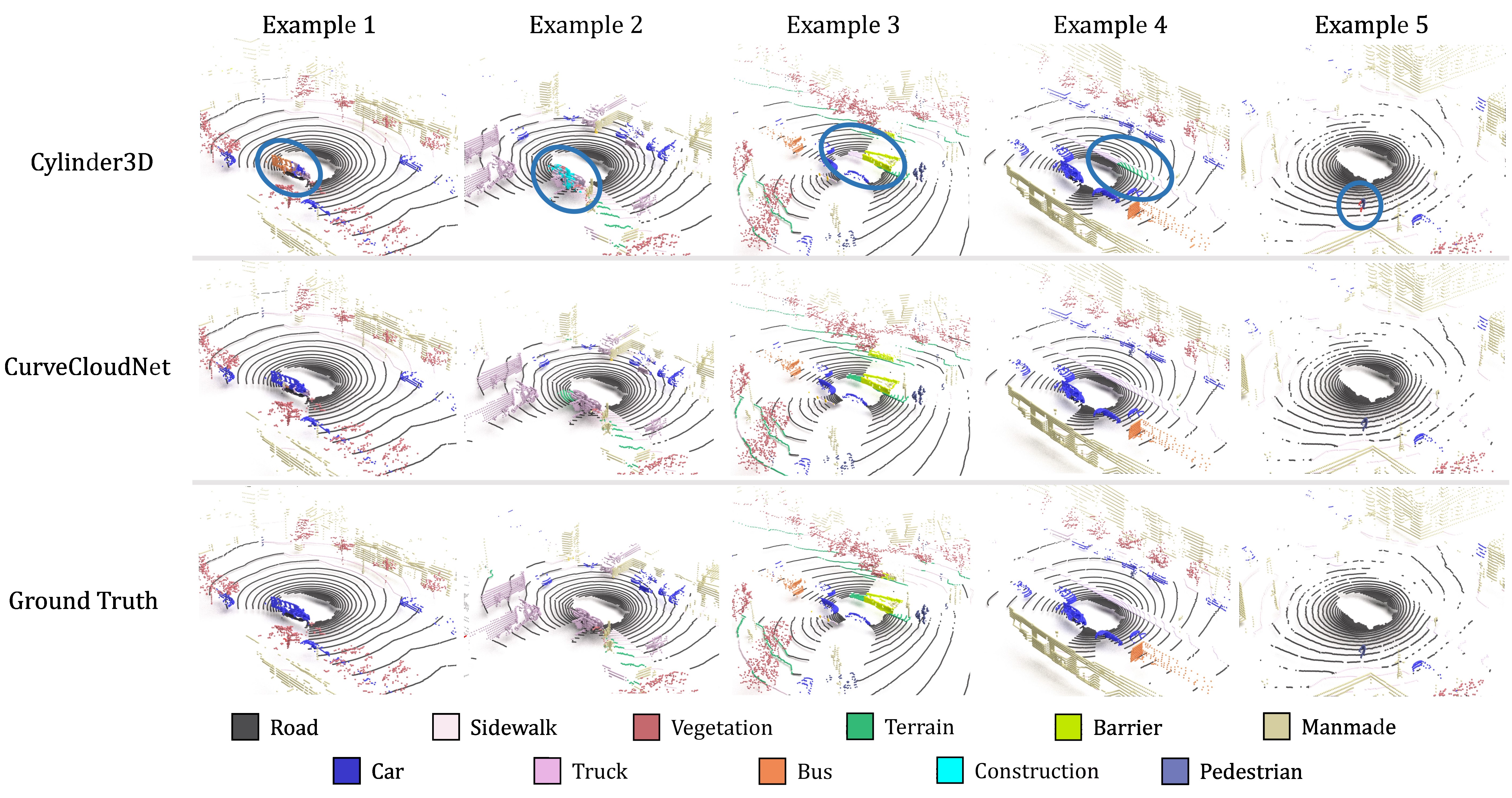
Figure S4: nuScenes Segmentation. We visualize semantic segmentation predictions of CurveCloudNet and Cylinder3D on the nuScenes validation split. We highlight regions where Cylinder3D errors and CurveCloudNet predicts correctly.

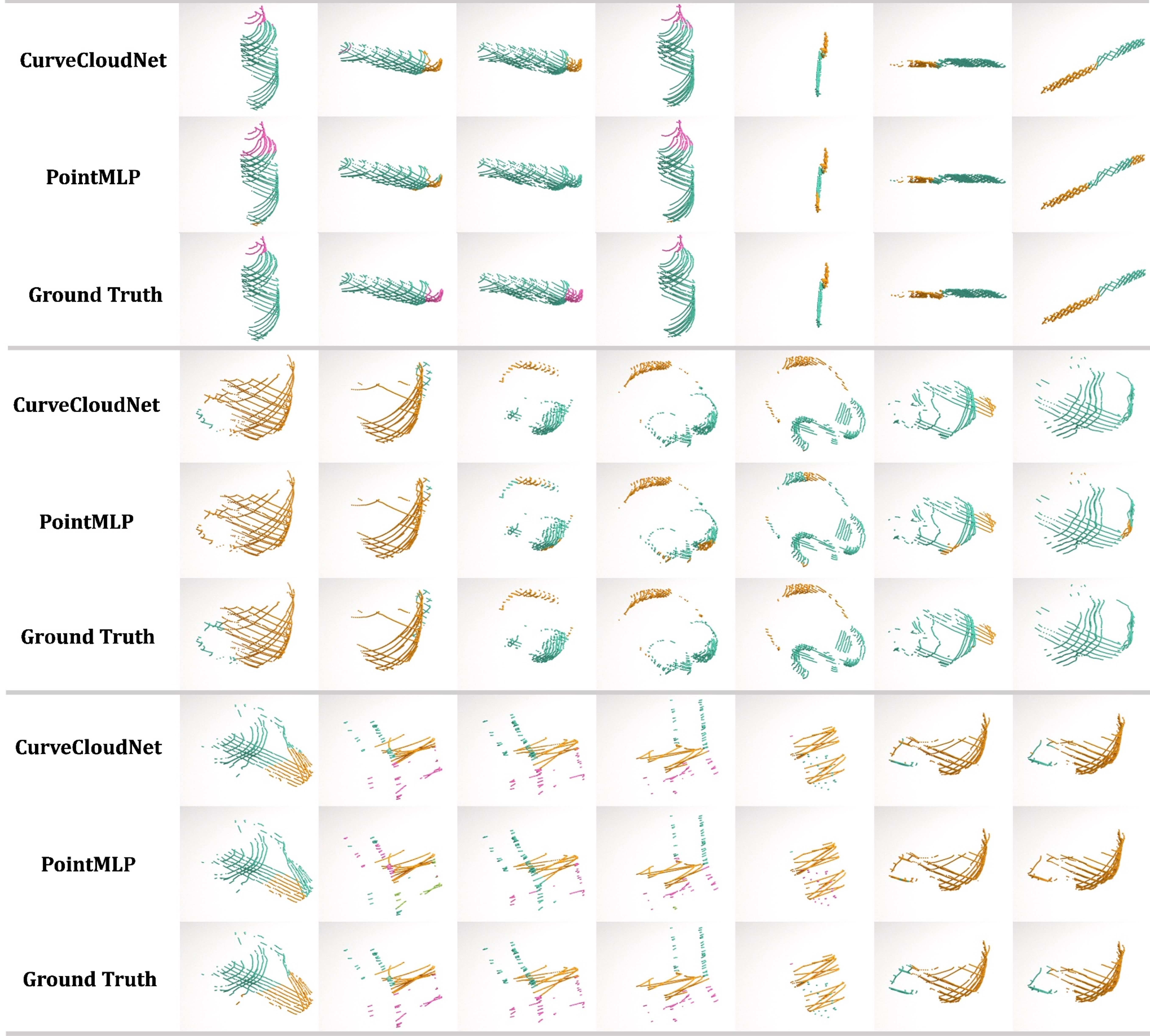
Figure S5: Kortx Dataset Part Segmentation. We visualize segmentation predictions of CurveCloudNet and PointMLP on the KortX dataset.

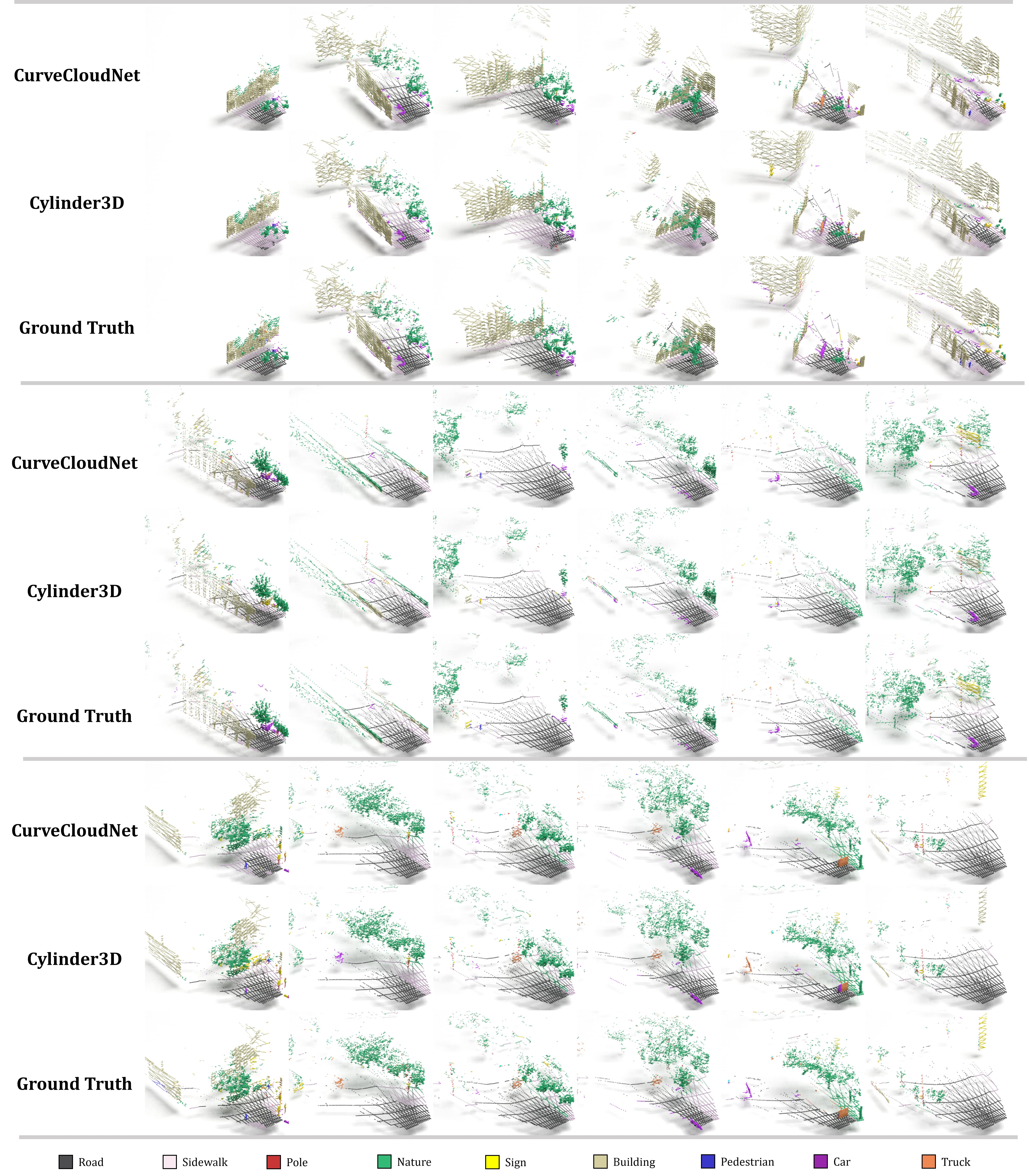
Figure S6: A2D2 Dataset Segmentation. We visualize segmentation predictions of CurveCloudNet and Cylinder3D on the A2D2 dataset.

References

- [1] Summer robotics. https://www.summerrobotics.ai/. Accessed: 2023-02-15.
- Ando et al. [2023] Angelika Ando, Spyros Gidaris, Andrei Bursuc, Gilles Puy, Alexandre Boulch, and Renaud Marlet. Rangevit: Towards vision transformers for 3d semantic segmentation in autonomous driving. 2023 IEEE/CVF Conference on Computer Vision and Pattern Recognition (CVPR), pages 5240–5250, 2023.
- Atzmon et al. [2018] Matan Atzmon, Haggai Maron, and Yaron Lipman. Point convolutional neural networks by extension operators. ACM Trans. on Graphics, 2018.
- Behley et al. [2019] J. Behley, M. Garbade, A. Milioto, J. Quenzel, S. Behnke, C. Stachniss, and J. Gall. SemanticKITTI: A Dataset for Semantic Scene Understanding of LiDAR Sequences. In Proc. of the IEEE/CVF International Conf. on Computer Vision (ICCV), 2019.
- Berman et al. [2018] Maxim Berman, Amal Rannen Triki, and Matthew B. Blaschko. The lovász-softmax loss: A tractable surrogate for the optimization of the intersection-over-union measure in neural networks. In Proc. IEEE Conf. on Computer Vision and Pattern Recognition (CVPR), 2018.
- Blelloch [1990] Guy E. Blelloch. Prefix sums and their applications. 1990.
- Boulch et al. [2020] Alexandre Boulch, Gilles Puy, and Renaud Marlet. Fkaconv: Feature-kernel alignment for point cloud convolution. 2020.
- Caesar et al. [2020] Holger Caesar, Varun Bankiti, Alex H Lang, Sourabh Vora, Venice Erin Liong, Qiang Xu, Anush Krishnan, Yu Pan, Giancarlo Baldan, and Oscar Beijbom. nuscenes: A multimodal dataset for autonomous driving. 2020.
- Chang et al. [2015a] Angel X. Chang, Thomas Funkhouser, Leonidas Guibas, Pat Hanrahan, Qixing Huang, Zimo Li, Silvio Savarese, Manolis Savva, Shuran Song, Hao Su, Jianxiong Xiao, Li Yi, and Fisher Yu. ShapeNet: An Information-Rich 3D Model Repository. Technical Report arXiv:1512.03012 [cs.GR], Stanford University — Princeton University — Toyota Technological Institute at Chicago, 2015a.
- Chang et al. [2015b] Angel X. Chang, Thomas A. Funkhouser, Leonidas J. Guibas, Pat Hanrahan, Qi-Xing Huang, Zimo Li, Silvio Savarese, Manolis Savva, Shuran Song, Hao Su, Jianxiong Xiao, Li Yi, and Fisher Yu. Shapenet: An information-rich 3d model repository. arXiv.org, 1512.03012, 2015b.
- Chen et al. [2020] Jintai Chen, Biwen Lei, Qingyu Song, Haochao Ying, Danny Z. Chen, and Jian Wu. A hierarchical graph network for 3d object detection on point clouds. In Proc. IEEE Conf. on Computer Vision and Pattern Recognition (CVPR), 2020.
- Cheng et al. [2022] Huimin Cheng, Xian-Feng Han, and Guoqiang Xiao. Cenet: Toward concise and efficient lidar semantic segmentation for autonomous driving. 2022 IEEE International Conference on Multimedia and Expo (ICME), pages 01–06, 2022.
- Cheng et al. [2021] Ran Cheng, Ryan Razani, Ehsan Moeen Taghavi, Enxu Li, and Bingbing Liu. (af)2-s3net: Attentive feature fusion with adaptive feature selection for sparse semantic segmentation network. 2021 IEEE/CVF Conference on Computer Vision and Pattern Recognition (CVPR), pages 12542–12551, 2021.
- Choy et al. [2019] Christopher B. Choy, JunYoung Gwak, and Silvio Savarese. 4d spatio-temporal convnets: Minkowski convolutional neural networks. In Proc. IEEE Conf. on Computer Vision and Pattern Recognition (CVPR), 2019.
- Eliasof and Treister [2020] Moshe Eliasof and Eran Treister. Diffgcn: Graph convolutional networks via differential operators and algebraic multigrid pooling. In Advances in Neural Information Processing Systems (NeurIPS), 2020.
- Esteves et al. [2018] Carlos Esteves, Christine Allen-Blanchette, Ameesh Makadia, and Kostas Daniilidis. Learning SO(3) equivariant representations with spherical cnns. In Proc. of the European Conf. on Computer Vision (ECCV), 2018.
- Fan et al. [2021] Hehe Fan, Yi Yang, and Mohan Kankanhalli. Point 4d transformer networks for spatio-temporal modeling in point cloud videos. In Proc. IEEE Conf. on Computer Vision and Pattern Recognition (CVPR), 2021.
- Fey and Lenssen [2019] Matthias Fey and Jan E. Lenssen. Fast graph representation learning with PyTorch Geometric. In ICLR Workshop on Representation Learning on Graphs and Manifolds, 2019.
- Geiger et al. [2012] Andreas Geiger, Philip Lenz, and Raquel Urtasun. Are we ready for autonomous driving? The KITTI vision benchmark suite. In Proc. IEEE Conf. on Computer Vision and Pattern Recognition (CVPR), 2012.
- Geyer et al. [2020] Jakob Geyer, Yohannes Kassahun, Mentar Mahmudi, Xavier Ricou, Rupesh Durgesh, Andrew S. Chung, Lorenz Hauswald, Viet Hoang Pham, Maximilian Mühlegg, Sebastian Dorn, Tiffany Fernandez, Martin Jänicke, Sudesh Mirashi, Chiragkumar Savani, Martin Sturm, Oleksandr Vorobiov, Martin Oelker, Sebastian Garreis, and Peter Schuberth. A2D2: audi autonomous driving dataset. arXiv.org, 2020.
- Graham et al. [2018] Benjamin Graham, Martin Engelcke, and Laurens van der Maaten. 3d semantic segmentation with submanifold sparse convolutional networks. In Proc. IEEE Conf. on Computer Vision and Pattern Recognition (CVPR), 2018.
- Gu et al. [2022] Yinjuan Gu, Yuming Huang, Chengzhong Xu, and Hui Kong. Maskrange: A mask-classification model for range-view based lidar segmentation. ArXiv, abs/2206.12073, 2022.
- Hou et al. [2022] Yuenan Hou, Xinge Zhu, Yuexin Ma, Chen Change Loy, and Yikang Li. Point-to-voxel knowledge distillation for lidar semantic segmentation. 2022 IEEE/CVF Conference on Computer Vision and Pattern Recognition (CVPR), pages 8469–8478, 2022.
- Hu et al. [2020] Qingyong Hu, Bo Yang, Linhai Xie, Stefano Rosa, Yulan Guo, Zhihua Wang, Niki Trigoni, and Andrew Markham. Randla-net: Efficient semantic segmentation of large-scale point clouds. In Proc. IEEE Conf. on Computer Vision and Pattern Recognition (CVPR), 2020.
- Hua et al. [2018] Binh-Son Hua, Minh-Khoi Tran, and Sai-Kit Yeung. Pointwise convolutional neural networks. In Proc. IEEE Conf. on Computer Vision and Pattern Recognition (CVPR), 2018.
- Ioffe and Szegedy [2015] Sergey Ioffe and Christian Szegedy. Batch normalization: Accelerating deep network training by reducing internal covariate shift. pages 448–456, 2015.
- Kingma and Ba [2015] Diederik P. Kingma and Jimmy Ba. Adam: A method for stochastic optimization. In Proc. of the International Conf. on Learning Representations (ICLR), 2015.
- Komarichev et al. [2019] Artem Komarichev, Zichun Zhong, and Jing Hua. A-CNN: annularly convolutional neural networks on point clouds. In Proc. IEEE Conf. on Computer Vision and Pattern Recognition (CVPR), 2019.
- Kong et al. [2023] Lingdong Kong, You-Chen Liu, Runnan Chen, Yuexin Ma, Xinge Zhu, Yikang Li, Yuenan Hou, Y. Qiao, and Ziwei Liu. Rethinking range view representation for lidar segmentation. ArXiv, abs/2303.05367, 2023.
- Lai et al. [2023] Xin Lai, Yukang Chen, Fanbin Lu, Jianhui Liu, and Jiaya Jia. Spherical transformer for lidar-based 3d recognition. In CVPR, 2023.
- Lan et al. [2019] Shiyi Lan, Ruichi Yu, Gang Yu, and Larry S Davis. Modeling local geometric structure of 3d point clouds using geo-cnn. In Proc. IEEE Conf. on Computer Vision and Pattern Recognition (CVPR), 2019.
- Lang et al. [2018] Alex H. Lang, Sourabh Vora, Holger Caesar, Lubing Zhou, Jiong Yang, and Oscar Beijbom. Pointpillars: Fast encoders for object detection from point clouds. 2019 IEEE/CVF Conference on Computer Vision and Pattern Recognition (CVPR), pages 12689–12697, 2018.
- Lei et al. [2019] Huan Lei, Naveed Akhtar, and Ajmal Mian. Octree guided CNN with spherical kernels for 3d point clouds. In Proc. IEEE Conf. on Computer Vision and Pattern Recognition (CVPR), 2019.
- Li et al. [2018] Jiaxin Li, Ben M Chen, and Gim Hee Lee. So-net: Self-organizing network for point cloud analysis. In Proc. IEEE Conf. on Computer Vision and Pattern Recognition (CVPR), 2018.
- Liu et al. [2019a] Jinxian Liu, Bingbing Ni, Caiyuan Li, Jiancheng Yang, and Qi Tian. Dynamic points agglomeration for hierarchical point sets learning. In Proc. of the IEEE International Conf. on Computer Vision (ICCV), 2019a.
- Liu et al. [2019b] Xinhai Liu, Zhizhong Han, Yu-Shen Liu, and Matthias Zwicker. Point2sequence: Learning the shape representation of 3d point clouds with an attention-based sequence to sequence network. In Proceedings of the AAAI conference on artificial intelligence, 2019b.
- Liu et al. [2019c] Yongcheng Liu, Bin Fan, Shiming Xiang, and Chunhong Pan. Relation-shape convolutional neural network for point cloud analysis. In Proc. IEEE Conf. on Computer Vision and Pattern Recognition (CVPR), 2019c.
- Liu et al. [2019d] Zhijian Liu, Haotian Tang, Yujun Lin, and Song Han. Point-voxel CNN for efficient 3d deep learning. In Advances in Neural Information Processing Systems (NeurIPS), 2019d.
- Liu et al. [2021] Zhijian Liu, Haotian Tang, Shengyu Zhao, Kevin Shao, and Song Han. Pvnas: 3d neural architecture search with point-voxel convolution. IEEE Transactions on Pattern Analysis and Machine Intelligence, 44:8552–8568, 2021.
- Ma et al. [2022] Xu Ma, Can Qin, Haoxuan You, Haoxi Ran, and Yun Fu. Rethinking network design and local geometry in point cloud: A simple residual mlp framework. In Proc. of the International Conf. on Learning Representations (ICLR), 2022.
- Mao et al. [2019] Jiageng Mao, Xiaogang Wang, and Hongsheng Li. Interpolated convolutional networks for 3d point cloud understanding. In Proc. of the IEEE International Conf. on Computer Vision (ICCV), 2019.
- Maturana and Scherer [2015] Daniel Maturana and Sebastian Scherer. Voxnet: A 3d convolutional neural network for real-time object recognition. In Proc. IEEE International Conf. on Intelligent Robots and Systems (IROS), 2015.
- Misra et al. [2021] Ishan Misra, Rohit Girdhar, and Armand Joulin. An end-to-end transformer model for 3d object detection. In Proc. of the IEEE International Conf. on Computer Vision (ICCV), 2021.
- Qi et al. [2016] C. Qi, Hao Su, Matthias Nießner, Angela Dai, Mengyuan Yan, and Leonidas J. Guibas. Volumetric and multi-view cnns for object classification on 3d data. 2016 IEEE Conference on Computer Vision and Pattern Recognition (CVPR), pages 5648–5656, 2016.
- Qi et al. [2017a] Charles R Qi, Hao Su, Kaichun Mo, and Leonidas J Guibas. Pointnet: Deep learning on point sets for 3d classification and segmentation. In Proc. IEEE Conf. on Computer Vision and Pattern Recognition (CVPR), 2017a.
- Qi et al. [2017b] Charles R Qi, Li Yi, Hao Su, and Leonidas J Guibas. Pointnet++: Deep hierarchical feature learning on point sets in a metric space. In Advances in Neural Information Processing Systems (NIPS), 2017b.
- Qian et al. [2022] Gordon Guocheng Qian, Yuchen Li, Houwen Peng, Jinjie Mai, Hasan Abed Al Kader Hammoud, Mohamed Elhoseiny, and Bernard Ghanem. Pointnext: Revisiting pointnet++ with improved training and scaling strategies. ArXiv, abs/2206.04670, 2022.
- Ravi et al. [2020] Nikhila Ravi, Jeremy Reizenstein, David Novotny, Taylor Gordon, Wan-Yen Lo, Justin Johnson, and Georgia Gkioxari. Accelerating 3d deep learning with pytorch3d. arXiv:2007.08501, 2020.
- Ronneberger et al. [2015] Olaf Ronneberger, Philipp Fischer, and Thomas Brox. U-net: Convolutional networks for biomedical image segmentation. In Medical Image Computing and Computer-Assisted Intervention (MICCAI), 2015.
- Shen et al. [2018] Yiru Shen, Chen Feng, Yaoqing Yang, and Dong Tian. Mining point cloud local structures by kernel correlation and graph pooling. In Proc. IEEE Conf. on Computer Vision and Pattern Recognition (CVPR), 2018.
- Su et al. [2018] Hang Su, Varun Jampani, Deqing Sun, Subhransu Maji, Evangelos Kalogerakis, Ming-Hsuan Yang, and Jan Kautz. Splatnet: Sparse lattice networks for point cloud processing. In Proc. IEEE Conf. on Computer Vision and Pattern Recognition (CVPR), 2018.
- Te et al. [2018] Gusi Te, Wei Hu, Amin Zheng, and Zongming Guo. RGCNN: regularized graph CNN for point cloud segmentation. In ACM Trans. on Graphics, 2018.
- Thomas et al. [2019] Hugues Thomas, Charles R. Qi, Jean-Emmanuel Deschaud, Beatriz Marcotegui, François Goulette, and Leonidas J. Guibas. Kpconv: Flexible and deformable convolution for point clouds. In Proc. of the IEEE International Conf. on Computer Vision (ICCV), 2019.
- Vaswani et al. [2017] Ashish Vaswani, Noam Shazeer, Niki Parmar, Jakob Uszkoreit, Llion Jones, Aidan N. Gomez, Lukasz Kaiser, and Illia Polosukhin. Attention is all you need. In Advances in Neural Information Processing Systems (NIPS), pages 5998–6008, 2017.
- Verma et al. [2018] Nitika Verma, Edmond Boyer, and Jakob Verbeek. Feastnet: Feature-steered graph convolutions for 3d shape analysis. In Proc. IEEE Conf. on Computer Vision and Pattern Recognition (CVPR), 2018.
- Wang et al. [2018] Shenlong Wang, Simon Suo, Wei-Chiu Ma, Andrei Pokrovsky, and Raquel Urtasun. Deep parametric continuous convolutional neural networks. In Proc. IEEE Conf. on Computer Vision and Pattern Recognition (CVPR), 2018.
- Wang and Solomon [2021] Yue Wang and Justin M. Solomon. Object DGCNN: 3d object detection using dynamic graphs. In Advances in Neural Information Processing Systems (NeurIPS), 2021.
- Wang et al. [2019a] Yue Wang, Yongbin Sun, Ziwei Liu, Sanjay E. Sarma, Michael M. Bronstein, and Justin M. Solomon. Dynamic graph CNN for learning on point clouds. ACM Trans. on Graphics, 2019a.
- Wang et al. [2019b] Ziyan Wang, Buyu Liu, Samuel Schulter, and Manmohan Chandraker. A parametric top-view representation of complex road scenes. In Proc. IEEE Conf. on Computer Vision and Pattern Recognition (CVPR), 2019b.
- Wiersma et al. [2022] Ruben Wiersma, Ahmad Nasikun, Elmar Eisemann, and Klaus Hildebrandt. Deltaconv: anisotropic operators for geometric deep learning on point clouds. ACM Trans. on Graphics, 2022.
- Wu et al. [2018] Bichen Wu, Alvin Wan, Xiangyu Yue, and Kurt Keutzer. Squeezeseg: Convolutional neural nets with recurrent CRF for real-time road-object segmentation from 3d lidar point cloud. In Proc. IEEE International Conf. on Robotics and Automation (ICRA), 2018.
- Wu et al. [2022a] Hai Wu, Jinhao Deng, Chenglu Wen, Xin Li, Cheng Wang, and Jonathan Li. Casa: A cascade attention network for 3-d object detection from lidar point clouds. IEEE Trans. Geosci. Remote. Sens., 2022a.
- Wu et al. [2022b] Hai Wu, Chenglu Wen, Wei Li, Xin Li, Ruigang Yang, and Cheng Wang. Transformation-equivariant 3d object detection for autonomous driving. arXiv.org, 2022b.
- Wu et al. [2019] Wenxuan Wu, Zhongang Qi, and Fuxin Li. Pointconv: Deep convolutional networks on 3d point clouds. In Proc. IEEE Conf. on Computer Vision and Pattern Recognition (CVPR), 2019.
- Wu et al. [2022c] Xiaoyang Wu, Yixing Lao, Li Jiang, Xihui Liu, and Hengshuang Zhao. Point transformer v2: Grouped vector attention and partition-based pooling. In NeurIPS, 2022c.
- Wu et al. [2022d] Xiaopei Wu, Liang Peng, Honghui Yang, Liang Xie, Chenxi Huang, Chengqi Deng, Haifeng Liu, and Deng Cai. Sparse fuse dense: Towards high quality 3d detection with depth completion. In Proc. IEEE Conf. on Computer Vision and Pattern Recognition (CVPR), 2022d.
- Xiang et al. [2021] Tiange Xiang, Chaoyi Zhang, Yang Song, Jianhui Yu, and Weidong Cai. Walk in the cloud: Learning curves for point clouds shape analysis. In Proc. of the IEEE International Conf. on Computer Vision (ICCV), 2021.
- Xie et al. [2018] Saining Xie, Sainan Liu, Zeyu Chen, and Zhuowen Tu. Attentional shapecontextnet for point cloud recognition. In Proc. IEEE Conf. on Computer Vision and Pattern Recognition (CVPR), 2018.
- Xu et al. [2020] Chenfeng Xu, Bichen Wu, Zining Wang, Wei Zhan, Peter Vajda, Kurt Keutzer, and Masayoshi Tomizuka. Squeezesegv3: Spatially-adaptive convolution for efficient point-cloud segmentation. In Proc. of the European Conf. on Computer Vision (ECCV), 2020.
- Xu et al. [2021a] Jianyun Xu, Ruixiang Zhang, Jian Dou, Yushi Zhu, Jie Sun, and Shiliang Pu. Rpvnet: A deep and efficient range-point-voxel fusion network for lidar point cloud segmentation. In Proc. of the IEEE International Conf. on Computer Vision (ICCV), 2021a.
- Xu et al. [2021b] Jianyun Xu, Ruixiang Zhang, Jian Dou, Yushi Zhu, Jie Sun, and Shiliang Pu. Rpvnet: A deep and efficient range-point-voxel fusion network for lidar point cloud segmentation. 2021 IEEE/CVF International Conference on Computer Vision (ICCV), pages 16004–16013, 2021b.
- Xu et al. [2021c] Mutian Xu, Runyu Ding, Hengshuang Zhao, and Xiaojuan Qi. Paconv: Position adaptive convolution with dynamic kernel assembling on point clouds. 2021c.
- Xu et al. [2018] Yifan Xu, Tianqi Fan, Mingye Xu, Long Zeng, and Yu Qiao. Spidercnn: Deep learning on point sets with parameterized convolutional filters. In Proc. of the European Conf. on Computer Vision (ECCV), 2018.
- Yan et al. [2020] Xu Yan, Jiantao Gao, Jie Li, Ruimao Zhang, Zhen Li, Rui Huang, and Shuguang Cui. Sparse single sweep lidar point cloud segmentation via learning contextual shape priors from scene completion. ArXiv, abs/2012.03762, 2020.
- Yan et al. [2022] Xu Yan, Jiantao Gao, Chaoda Zheng, Chaoda Zheng, Ruimao Zhang, Shenghui Cui, and Zhen Li. 2dpass: 2d priors assisted semantic segmentation on lidar point clouds. In European Conference on Computer Vision, 2022.
- Yan et al. [2018] Yan Yan, Yuxing Mao, and Bo Li. Second: Sparsely embedded convolutional detection. Sensors, 2018.
- Yang et al. [2022] Bangbang Yang, Chong Bao, Junyi Zeng, Hujun Bao, Yinda Zhang, Zhaopeng Cui, and Guofeng Zhang. Neumesh: Learning disentangled neural mesh-based implicit field for geometry and texture editing. In Proc. of the European Conf. on Computer Vision (ECCV), 2022.
- Yang et al. [2019] Jiancheng Yang, Qiang Zhang, Bingbing Ni, Linguo Li, Jinxian Liu, Mengdie Zhou, and Qi Tian. Modeling point clouds with self-attention and gumbel subset sampling. In Proc. IEEE Conf. on Computer Vision and Pattern Recognition (CVPR), 2019.
- Yang et al. [2020] Zetong Yang, Yanan Sun, Shu Liu, and Jiaya Jia. 3dssd: Point-based 3d single stage object detector. 2020 IEEE/CVF Conference on Computer Vision and Pattern Recognition (CVPR), pages 11037–11045, 2020.
- Yi et al. [2016] Li Yi, Vladimir G Kim, Duygu Ceylan, I-Chao Shen, Mengyan Yan, Hao Su, Cewu Lu, Qixing Huang, Alla Sheffer, and Leonidas Guibas. A scalable active framework for region annotation in 3d shape collections. ACM Transactions on Graphics (ToG), 2016.
- Zhang et al. [2022a] Cheng Zhang, Haocheng Wan, Xinyi Shen, and Zizhao Wu. Pvt: Point-voxel transformer for point cloud learning. arXiv.org, 2022a.
- Zhang and Xiao [2019] Wenxiao Zhang and Chunxia Xiao. PCAN: 3d attention map learning using contextual information for point cloud based retrieval. In Proc. IEEE Conf. on Computer Vision and Pattern Recognition (CVPR), 2019.
- Zhang et al. [2020] Yang Zhang, Zixiang Zhou, Philip David, Xiangyu Yue, Zerong Xi, Boqing Gong, and Hassan Foroosh. Polarnet: An improved grid representation for online lidar point clouds semantic segmentation. In Proc. IEEE Conf. on Computer Vision and Pattern Recognition (CVPR), 2020.
- Zhang et al. [2022b] Yifan Zhang, Qingyong Hu, Guoquan Xu, Yanxin Ma, Jianwei Wan, and Yulan Guo. Not all points are equal: Learning highly efficient point-based detectors for 3d lidar point clouds. In Proc. IEEE Conf. on Computer Vision and Pattern Recognition (CVPR), 2022b.
- Zhao et al. [2021a] Hengshuang Zhao, Li Jiang, Jiaya Jia, Philip H. S. Torr, and Vladlen Koltun. Point transformer. In Proc. of the IEEE International Conf. on Computer Vision (ICCV), 2021a.
- Zhao et al. [2021b] Yiming Zhao, Lin Bai, and Xinming Huang. Fidnet: Lidar point cloud semantic segmentation with fully interpolation decoding. 2021 IEEE/RSJ International Conference on Intelligent Robots and Systems (IROS), pages 4453–4458, 2021b.
- Zhou et al. [2020] Hui Zhou, Xinge Zhu, Xiao Song, Yuexin Ma, Zhe Wang, Hongsheng Li, and Dahua Lin. Cylinder3d: An effective 3d framework for driving-scene lidar semantic segmentation. arXiv.org, 2020.
- Zhou et al. [2018] Qian-Yi Zhou, Jaesik Park, and Vladlen Koltun. Open3D: A modern library for 3D data processing. arXiv:1801.09847, 2018.