Large-Scale Traffic Signal Control Using Constrained Network Partition and Adaptive Deep Reinforcement Learning

Abstract

Multi-agent Deep Reinforcement Learning (MADRL) based traffic signal control becomes a popular research topic in recent years. To alleviate the scalability issue of completely centralized RL techniques and the non-stationarity issue of completely decentralized RL techniques on large-scale traffic networks, some literature utilizes a regional control approach where the whole network is firstly partitioned into multiple disjoint regions, followed by applying the centralized RL approach to each region. However, the existing partitioning rules either have no constraints on the topology of regions or require the same topology for all regions. Meanwhile, no existing regional control approach explores the performance of optimal joint action in an exponentially growing regional action space when intersections are controlled by 4-phase traffic signals (EW, EWL, NS, NSL). In this paper, we propose a novel RL training framework named RegionLight to tackle the above limitations. Specifically, the topology of regions is firstly constrained to a star network which comprises one center and an arbitrary number of leaves. Next, the network partitioning problem is modeled as an optimization problem to minimize the number of regions. Then, an Adaptive Branching Dueling Q-Network (ABDQ) model is proposed to decompose the regional control task into several joint signal control sub-tasks corresponding to particular intersections. Subsequently, these sub-tasks maximize the regional benefits cooperatively. Finally, the global control strategy for the whole network is obtained by concatenating the optimal joint actions of all regions. Experimental results demonstrate the superiority of our proposed framework over all baselines under both real and synthetic datasets in all evaluation metrics.

I Introduction

Traffic congestion is becoming a significant problem that lead to both financial costs and environmental damage. According to a recent study, traffic congestion costs £595 and 73 hours per driver in the UK [1] while drivers in the USA spent $ 564 each and wasted 3.4 billion hours a year in total [2]. Meanwhile, the gas emission caused by traffic congestion is now an unignorable contributor to the pollutants responsible for air pollution [3]. Therefore, there is an urgent need to apply effective strategies to relieve urban traffic congestion.

Traffic signal control (TSC) is an efficient and direct way to reduce traffic congestion by managing and regulating the movements of vehicles[4]. Existing TSC strategies can be generally classified into two categories: classical methods and AI (Artificial Intelligence) -based methods. Classical methods take rule-based signal plans such as Webster [5, 6] and MaxBand [7] which compute optimal signal plans based on traffic parameters such as traffic demand and saturation rate. However, most classical methods assume that traffic flow is uniform and traffic signals share the same cycle length and they hardly adapt to more complex traffic dynamics in real scenarios. Therefore, some adaptive rule-based methods such as Max-pressure[8] and self-organizing traffic lights (SOTL)[9, 10, 11] have been proposed to control traffic signals based on real-time information. Inspired by nature, meta-heuristics methods have been applied to solve traffic signal control problems in an evolutionary and long-sighted manner[12, 13]. Among various categories in meta-heuristics methods, genetic algorithms[14], artificial bee colony algorithms[15], and harmony search algorithms[16] are three common population-based methods and they have been successfully applied to traffic networks with various scales and demands[17, 18, 19, 20].

In recent years, AI-based methods especially deep reinforcement learning (DRL) techniques become very popular in sequential decision-making problems due to the huge achievement and success in both reinforcement learning (RL) and deep neural network (DNN)[21, 22, 23, 24]. There is already considerable literature applying DRL techniques to TSC applications and showing its advantages over the classical methods[25, 26, 27]. In early research work, the completely centralized RL technique, where one single agent controls the signal settings of all intersections in traffic grid networks, can learn the optimal policy and achieve a good convergence rate when the size of the traffic network is moderate [25, 26, 27]. However, this technique suffers from the scalability issue and is computationally impractical when the size of the traffic network becomes large [28]. The completely decentralized technique, where each intersection is assigned to one agent, can overcome the scalability issue by learning the optimal signal control policy either independently or cooperatively [29]. However, MADRL can cause the non-stationarity issue because the transition of the environment is affected by the joint actions of all agents. The independent RL technique, which maximizes each agent’s own reward without considering the change of environment caused by other agents, may fail to converge theoretically[30]. In contrast, the cooperative RL technique aims to maximize not only individual rewards but also local or global rewards. Large amounts of work have proposed cooperative RL methods by either applying communication protocols or coordination strategies between agents[31, 32, 33]. Nonetheless, the non-stationary issue may still lead to suboptimal control or even convergence failure when the number of agents is large [34].

To achieve a trade-off between scalability and optimality, some literature has applied a compromised technique which normally involves two stages[35, 36] where the first stage is to partition a large network into several disjoint small regions and each region is composed of a set of intersections, followed by applying the centralized RL technique to control each region. The global joint action of the whole network is a concatenation of the local action of each region. However, existing approaches still have the following limitations:

• Regions with identical topology may fail to adapt to a different network with a new distribution of intersections’ degree and some networks cannot even be partitioned into multiple regions with identical topology. Although the regions in [35] are partitioned dynamically based on real-time traffic density, the traffic dynamics for regions with the same size but different topologies may differ. Therefore, regions of identical topology lack adaptability, and regions with unrestricted topology may be difficult for RL agents to learn regional traffic dynamics.

• Since each region is controlled by one centralized agent, the challenge of optimal joint action searching for the region is naturally inherited from the completely centralized RL technique. Suppose there are $N$ traffic signals and each signal has $k$ phases, then the size of joint action space is $N^{k}$. As the number of intersections increases, the cardinality of regional joint action space grows exponentially. Hence, the size of the output layer in deep Q-network (DQN) and that in the actor-network of actor-critic architecture also grow exponentially. Besides, existing work bound the size of joint action space by considering traffic signals with two phases but urban traffic signals usually have four phases. Thus, the efficiency of searching for the optimal action for a region needs careful investigation.

To overcome the above limitations, we propose a constrained partitioning rule and extend Branching Dueling Q-Network (BDQ), whose output layer size grows linearly, with an adaptive computation of target value. More specifically, our main contributions are listed as follows:

1. We propose a shape-free network partitioning rule which can adapt to networks with different distributions of intersections’ degrees. The disjoint region under our partitioning rule includes a central intersection and a subset of its neighboring intersections. Therefore, the maximum distance between any pair of intersections is two inside the region and the topology of the region under the above constraint is a star in graph theory. We further model the network partitioning problem as an optimization problem to minimize the number of regions and give a theoretical analysis of the uniqueness of regions. For those intersections with less than four neighbors, fictitious intersections are introduced to fill the absence during training. Here we define that a region is fully loaded if there is no fictitious intersection in this region. Otherwise, this region is partially loaded.

2. We propose Adaptive BDQ (ABDQ) in which the computation of target value and loss adaptively involves only non-fictitious intersections for different regions in order to mitigate the negative influence of fictitious intersections. Since the location of fictitious intersections varies across regions, experimental results show that ADBQ has the potential to control a different number of intersections even in non-grid traffic networks.

3. We evaluate our framework on both real and synthetic datasets. Experimental results show that, although there is no coordination or communication considered among our regional agents, the performance of the proposed approach is better than all baselines. The robustness of our partitioning rule is further examined by employing different region configurations and trying different assignment orders. Also, ABDQ is applied to $2\times 3$ regions to demonstrate its advantage on partially loaded regions.

The rest of the paper is arranged as follows: Section II discusses the related work. Section III introduces the background and notations of traffic signal control and MARL. Section IV presents our network partitioning rule and the formulation of our regional agents. Section V describes the setting of experiments and discusses the results. Section VI summarises this paper.

II Related Work

In this section, we review and summarize the related work in DRL-based traffic signal control. In recent decades, more researchers have realized that only individual information from a single intersection is not enough to design intelligent signal controllers in large transport systems and have started to utilize local or even global information. The most straightforward way is to use a single agent to control all signals with the global information of the traffic network [25, 26, 27]. Although this strategy shows a convergence advantage in small-size traffic networks, it suffers from the scalability issue which leads to a poor convergence rate in large-scale traffic networks [28]. Till now, lots of MADRL algorithms adopting the completely decentralized technique have been proposed to coordinate the action of agents. Van der Pol et al. [31] modeled the traffic network as a linear combination of each intersection and applied the max-plus algorithm[37] to select joint actions. In [38], according to the congestion level between the intersection and its neighborhood, the agent can either follow a greedy policy to maximize individual rewards or Neighborhood Approximate Q-Learning to maximize local rewards.

Meanwhile, either explicitly or implicitly information-sharing protocols among completely decentralized agents have been studied in some existing literature. Arel et al. [39] proposed the NeighbourRL in which the observation of one agent is concatenated with the state of the neighboring intersections. Varaiya [8] proposed the Max-pressure scheme which considers the difference between the number of waiting vehicles of upstream intersections and that of downstream intersections, and this idea was further applied in PressLight[40]. In CoLight[41], a Graph Attention Network (GAN) was applied to augment the observation of each agent with a dynamically weighted average of its neighboring agents’ observations. In contrast, Wang et al. combined GAN with an Actor-critic framework to embed the state of neighboring intersections dynamically[42]. Graph Convolutional Reinforcement Learning[43] can learn underlying relations between neighboring agents and Graph Convolutional Networks (GCN) have also been applied to automatically capture the geometric feature among neighboring intersections[44]. Similarly, Devailly et al. proposed inductive graph reinforcement learning where inductive learning and four different types of nodes corresponding to TSC, connection, lane, and vehicle are modeled to support the learning of the surrounding environment and to improve transferability[45]. To speed up the training process, Zang et al. [46] proposed a meta-learning framework named MetaLight to enhance the adaptive ability of RL learning to a new environment by reusing and transferring old experiences. Wang et al. [33] proposed cooperative double Q-learning (Co-DQL) in which the Q-values of agents converge to Nash equilibrium. In their work, the state of one intersection is concatenated with the average value of its neighboring intersections while the reward of one intersection is summed with a weight-average of rewards of its neighboring intersections. Zhang et al.[32] proposed neighborhood cooperative hysteretic DQN (NC-HDQN) which studies the correlations between neighboring intersections. In their work, two methods are designed to calculate the correlation degrees of intersection. The first method, named empirical NC-HDQN (ENC-HDQN), assumes that the correlation degrees of two intersections are positively related to the number of vehicles moving between two intersections. In ENC-HDQN, the correlation degrees are always positive and the threshold is manually defined according to the demand of traffic flow. The other method named Pearson NC-HDQN (PNC-HDQN) stores reward trajectories of each intersection and computes Pearson correlation coefficients based on those history trajectories. Unlike ENC-HDQN, PNC-HDQN allows negative correlation degrees between intersections. With correlation degrees of neighboring intersections, the reward of one intersection is summed with its neighboring intersections’ rewards weighted by correlation degrees respectively. In ENC-HDQN, the weighted sum of rewards can be interpreted as different levels of competition as the coefficients are non-negative. In PNC-HDQN, negative coefficients might be interpreted as cooperation between intersections. In [47], the traffic grid network was firstly decomposed into several sub-networks based on the level of connectivity and average residual capacity. Then, all decentralized agents in each sub-network share state and reward.

Apart from the completely decentralized technique, some literature applies the regional control technique. In [35], sub-networks are firstly initialized based on the real-time traffic density between adjacent intersections and further partitioned into small disjoint regions with normalized-cut algorithm [48] in network theory. Then, approximate Q-Learning is applied to search for sub-optimal actions for all regions. In [36], a $4\times 6$ traffic grid is partitioned into four $2\times 3$ disjoint regions and controlled in a decentralized-to-centralized manner by regional DRL (R-DRL) agents and one global coordinator. In R-DRL, deep deterministic policy gradient (DDPG) and Wolpertinger Architecture (WA) are applied to search for the optimal action for each region through three steps. Firstly, the actor generates a proto-action in continuous space. Secondly, the $K$-nearest-neighbour (KNN) algorithm is applied to map proto-action to $K$ actions in discrete space. Finally, the critic evaluates the optimal action among $K$ actions. The larger the $K$ is, the higher chance the optimal action is in $K$ actions. Therefore, this search method heavily depends on the choice of $K$ and $K$ is suggested to be proportional to the cardinality of regional joint action space in practice. To achieve better cooperation among R-DRL agents, a global coordinator is applied to achieve coordinated R-DRL agents by combining an iterative action search algorithm and one global Q-value estimator. In the iterative action search algorithm, each agent proposes its local optimum actions. Then, from this initial joint action search point, each agent iteratively chooses whether to deviate from its local optimum actions according to the Q-value computed by the global Q-value estimator. Although the iterative search approach offers sufficient trials for different sets of joint actions, the performance of the iterative search approach heavily depends on the convergence of the global function, and the assumption that the global function is well-learned is still too strong for large-scale traffic networks.

III Background

III-A Traffic Signal Control Definition

Let us define a traffic network as a directional graph $\mathcal{G}=(\mathcal{V},\mathcal{E})$ where $v\in\mathcal{V}$ represents an intersection and $e_{vu}=(v,u)\in\mathcal{E}$ represents the adjacency and connection between two intersections. The neighborhood of intersection $v$ is denoted as $NB_{v}=\{u|(v,u)\in\mathcal{E}\}$ and the degree of one intersection is the size of its neighborhood. $d(v,u)$ denotes the minimum number of edges to connect two intersections $v,u$.

There are two types of approaches for each intersection: The incoming approach is the approach on which vehicles enter the intersection and the outgoing approach is the approach on which vehicles leave the intersection. Each approach consists of a number of lanes and there are incoming lanes and outgoing lanes. The set of entering lanes of intersection $v$ is denoted as $Lane[v]$. A traffic movement is defined as a pair of one incoming lane and one outgoing lane. A phase is a combination of traffic movements that are set to be green. As illustrated right side in Fig. 1, one intersection has four phases which are North-South Straight (NS), North-South Left-turn (NSL), East-West Straight (EW), and East-West Left-turn (EWL).

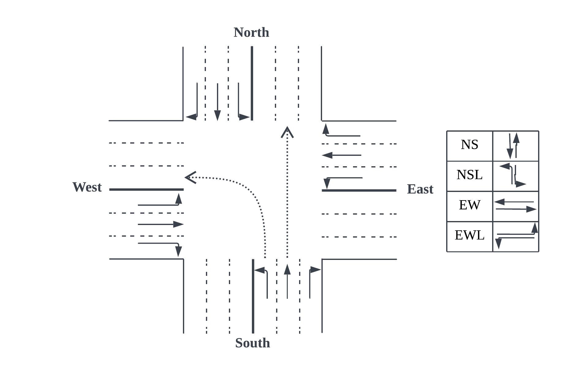
Figure 1: Traffic network example

TABLE I: Notion Table

$\mathcal{V}$	set of all intersections
$\mathcal{E}$	set of all approaches
$NB_{v}$	neighborhood intersections of $v$
$d(v,u)$	minimum hops between $v$ and $u$
$Lane[v]$	entering lanes of intersection $v$
$wait[l]$	number of waiting vehicles on lane $l$
$wave[l]$	number of vehicles on lane $l$
$phase[v]$	the phase of intersection $v$

III-B Markov Game Framework

Multi-agent system is usually modelled as a Markov Game (MG) [49] which is defined as a tuple$\langle\mathcal{N},\mathcal{S},\mathcal{O},\mathcal{A},R,P,\gamma\rangle$ where $\mathcal{N}$ is the agent space, $\mathcal{S}$ is the state space, $\mathcal{O}=\{\mathcal{O}_{1},...,\mathcal{O}_{|\mathcal{N}|}\}$ is the observation space and $\mathcal{O}_{i}$ of agent $i$ is observed partially from the state of the system, $\mathcal{A}=\{\mathcal{A}_{1},...,\mathcal{A}_{|\mathcal{N}|}\}$ is the joint action space of all agents, $r_{i}\in R:\mathcal{O}_{i}\times\mathcal{A}_{1}\times\cdots\times\mathcal{A}_{|\mathcal{N|}}\rightarrow\mathbb{R}$ maps an observation-action pair to a real number, $P:\mathcal{S}\times\mathcal{A}_{1}\times\cdots\times\mathcal{A}_{|\mathcal{N}|}\times\mathcal{S}\rightarrow[0,1]$ is the transition probability space that assigns a probability to each state-action-state transition and $\gamma$ is the reward discounted factor.

The goal of MG is to find a joint optimal policy $\pi^{*}=\{\pi^{*}_{1},...,\pi^{*}_{|\mathcal{N}|}\}$ under which each agent $i$ maximizes its own expected cumulative reward

$$\mathbb{E}_{\pi_{i}}[\sum_{k=0}^{\infty}\gamma^{k}r_{i,t+k}|o_{i}]$$ (1)

where $\pi_{i}$ : $\mathcal{O}_{i}\times\mathcal{A}_{i}\rightarrow[0,1]$ maps the observation of agent $i$ to the probability distribution of its action. The action-value (Q-value) of agent $i$ is defined as $Q_{i}(o_{i},a_{i})=\mathbb{E}_{\pi_{i}}[\sum_{k=0}^{\infty}\gamma^{k}r_{i,t+k}|o_{i},a_{i}]$. Tabular Q-learning is a classic algorithm to learn and store action-value [50]. The update rule is formulated as

$$Q_{i}(o_{i},a_{i})=Q_{i}(o_{i},a_{i})+\alpha(y-Q_{i}(o_{i},a_{i}))$$ (2)

where $\alpha$ is the learning rate and

$$y=r_{i}+\gamma\max_{a_{i}\in\mathcal{A}_{i}}Q_{i}(o_{i}^{\prime},a_{i})$$ (3)

III-C Branching Dueling Q-Network

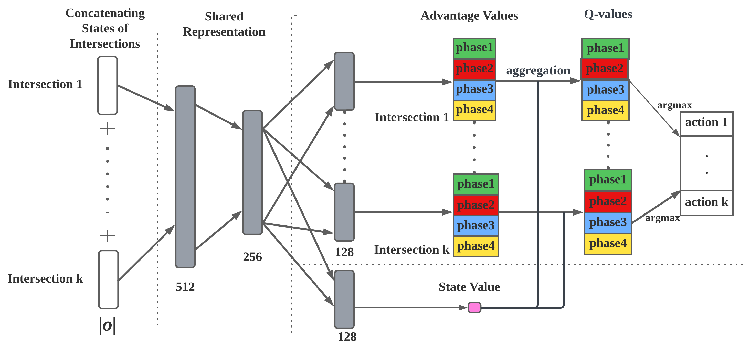
Figure 2: Structure of BDQ. Firstly, the states of intersections are concatenated into a vector and embedded through fully connected layers. Then, the last hidden layer of shared representation is used for both calculations of advantage values and the state value. Next, through the aggregation layer, Q-values of all action branches are calculated with advantage values and the state value based on Eq. (4). The size of each layer is annotated below.

In some complex real-life tasks such as robotic control, one task may be divided into several sub-tasks and each sub-task contains a different number of actions. Consequently, the size of the action space grows exponentially and the evaluation of each sub-action becomes complex. To improve the efficiency of optimal joint action searching and coordinate sub-tasks to reach a global goal, Travakoli et al. proposed a novel agent BDQ [51] to reduce the output size of the neural network while holding a good convergence property. Suppose that an agent controls $K$ intersections and each intersection has $|\mathcal{A}_{k}|$ actions, then the cardinality of the action space of this agent is $\prod_{k\in K}|\mathcal{A}_{k}|$. However, the size of the output of DQN grows exponentially while that of BDQ grows linearly (Fig. 2).

As illustrated in Fig. 2, suppose one RL agent controls $k$ traffic signals and the state dimension $|s_{v}|$ of each intersection $v$ is the same, then the input layer is a concatenated vector $R^{|\mathcal{O}|\times 1}$ where $|\mathcal{O}|=|s_{v}|k$. Then the input vector is embedded through two fully connected layers as shared representation layers. The last shared representation layer is first used to compute a common state value and then embedded to get advantage values of each action branch independently. Then, the advantage values of each action branch are further aggregated with the state value to calculate the Q-values of each action branch. In [51], three ways are proposed to aggregate Q-values and we select the mean advantage aggregation for better stability as the original paper suggested. Formally, suppose that there are $K$ action branches and each action branch has $|\mathcal{A}_{k}|$ sub-actions, The Q-value of one sub-action is calculated by the common state value and the advantage of this sub-action over the average performance of all sub-actions in this action branch, i.e.,

$$Q_{k}(s,a_{k})=V(s)+(A_{k}(s,a_{k})-\frac{1}{n}\sum_{a^{{}^{\prime}}_{k}\in\mathcal{A}_{k}}(A_{k}(s,a^{\prime}_{k})))$$ (4)

To compute the temporal difference target, we choose the mean operator to coordinate all branches to reach a global learning target, i.e.,

$$y=r+\gamma\frac{1}{N}\sum_{k}Q^{-}_{k}(s^{\prime},\underset{a^{{}^{\prime}}_{k}\in\mathcal{A}_{k}}{\text{arg max}}Q_{k}(s^{\prime},a_{k}^{\prime}))$$ (5)

Based on Eq. (4) and Eq. (5), the loss function can be obtained by

$$L=\mathbb{E}_{(s,a,r,s^{\prime})\sim D}[\frac{1}{N}\sum_{k}(y_{k}-Q_{k}(s,a_{k})^{2}]$$ (6)

IV Constrained Network Partition and Formulation of Regional Agent

In this section, we present our partitioning rules for regions and the formulation of regional RL agents. Previous research has demonstrated the benefits of observing either partial or complete states of neighboring intersections [39, 32, 33]. Inspired by these work, we assume that an agent can observe the state of all intersections in the corresponding region. We also assume that each intersection has at most four neighbors and this assumption can be trivially extended to networks where the maximum degree is larger than four.

IV-A Network Partitioning Rule

A region $I_{v}=\{v\cup U\}$ where $U\subseteq NB_{v}$ is a set of intersections including $v$ and a subset of its adjacent intersections. Region configuration $I$ is a union of several regions and follows two constraints :

$$\cup_{v}I_{v} =\mathcal{V}$$ (7)

$$I_{v}\cap I_{u} =\emptyset,\forall I_{v},I_{u}$$ (8)

These two constraints ensure that all regions are disjoint and each intersection is only assigned to one region.

IV-B Optimization Problem and Region Construction

The purpose of regional control is to alleviate the non-stationary issue by restricting the number of agents. Therefore, based on the above two constraints in Eq. (7) and (8), we further model the network partitioning problem as the dominating set problem [52] and construct the region configuration based on the minimum dominating set which is defined as follows.

Definition 1 (Dominating Set and Domination Number).

A set $W\subseteq\mathcal{V}$ is a dominating set if every intersection $v\in\mathcal{V}\setminus W$ has a neighbor in $W$. The domination number $\gamma(\mathcal{G})$ is the minimum size of a dominating set in $\mathcal{G}$. The minimum dominating set is a dominating set of size $\gamma(\mathcal{G})$.

Remark 1.

The union of centers of all regions $W=\cup_{I_{v}}\{v\}$ is a dominating set.

Therefore, minimizing the number of regions is equivalent to solving the domination number and the minimum dominating set. However, the problems to solve the domination number and find the corresponding dominating set are $NP$-Hard[53]. So we formulate an integer programming problem to solve the optimization problem [54]. We assign one binary decision variable $x_{v}$ to each intersection $v\in\mathcal{V}$. Intersection $v$ is a center if its corresponding variable $x_{v}=0$. Otherwise, it is a leaf. Formally, the cost function and constraints are:

$$\max\quad \sum_{v\in\mathcal{V}}x_{v}$$ (9)

s.t. $$\sum_{u\in NB_{v}}x_{u}+x_{v}\leq|NB_{v}|,\quad\forall v\in\mathcal{V}$$ (10)

$$x_{v}=0\quad\text{or}\quad 1,\quad\forall v\in\mathcal{V}$$ (11)

The objective to minimize the size of dominating set is equivalent to maximizing the number of leaves. Therefore, Eq. (9) is satisfied. To formulate the constraints to meet Definition 1, we use binary variables to represent the leaf or center and consider two situations. If one intersection $v$ is a leaf, then at least one of its neighboring intersections is a center. So the sum of decision variables of its neighboring intersections should be less than the number of its neighboring intersections, i.e.,

$$\sum_{u\in NB_{v}}x_{u}<|NB_{v}|,\quad x_{v}=1\\$$ (12)

Since all variables are binary, we can re-write Eq. (12) into

$$\sum_{u\in NB_{v}}x_{u}\leq|NB_{v}|-1,\quad x_{v}=1$$ (13)

$$\iff \sum_{u\in NB_{v}}x_{u}+x_{v}\leq|NB_{v}|,\quad x_{v}=1$$ (14)

Eq. (14) holds because the value of $x_{v}$ is a constant value in this constraint. If one intersection $v$ is a center, then there is no constraint on its neighboring intersections.

$$\sum_{u\in NB_{v}}x_{u}+x_{v}\leq|NB_{v}|,\quad x_{v}=0$$ (15)

Meanwhile, the Eq. (15) holds trivially. As a result, the combination of Eq. (14) and (15) leads to the constraint condition shown in Eq. (10). Therefore, the integer programming formulation from Eq. (9) to (11) is verified. After solving the optimization problem, we can get the minimum dominating set $W=\{v|x_{v}=0,v\in\mathcal{V}\}$. Based on each center, we can construct region configurations around each center (Algorithm 1).

Algorithm 1 Construction of Region Configuration

1:Input graph $\mathcal{G}$, minimum dominating set $W$

2:Initialise $key$ to track the assignment of intersection

3:Initialise $I$ to store the configuration of regions

4:for each $v$ in $\mathcal{V}$ do

5:     if $v\in W$ then

6:         $I[v]\leftarrow\{v\}$ $\triangleright$ initialise region centered at $v$

7:         $key[v]\leftarrow 1$ $\triangleright$ mark $v$ is assigned

8:     else

9:         $I[v]\leftarrow\emptyset$

10:         $key[v]\leftarrow 0$

11:     end if

12:end for

13:for each $v$ in $W$ do $\triangleright$ construct regions iteratively

14:     for each $u$ in $NB_{v}$ do

15:         if $key[u]=0$ then

16:              $I[v]\leftarrow I[v]\cup u$ $\triangleright$ $u$ is assigned to $I[v]$

17:              $key[u]\leftarrow 1$ $\triangleright$ mark $u$ is assigned

18:         end if

19:     end for

20:end for

21:return $I$

In Algorithm 1, line 16 ensures that all intersections are assigned to one region in order to satisfy the first constraint in Eq. (7), and line 17 ensures that each intersection is assigned to exactly one region to satisfy the second constraint in Eq. (8). However, Algorithm 1 can only construct one region configuration when there exists that a leaf intersection has two alternative neighboring centers. Next, we discuss the uniqueness of the region configuration under Algorithm 1 based on one minimum dominating set.

Theorem 1.

If, $\forall v,u\in W,d(v,u)\geq 3$, then the region configuration $I=\cup_{v\in W}\{I_{v}\}$ where $I_{v}=\{NB_{v}\cup v\}$ is unique.

Lemma 1.

$\forall v,u\in W,(NB_{v}-u)\cap(NB_{u}-v)=\emptyset$ iff $\forall z\in\mathcal{V}\setminus W$, $|NB_{z}\cap W|=1$

Proof for Lemma 1.

We first prove only if part of the lemma by contraposition. Assume that $\exists z\in\mathcal{V}\setminus W\text{ such that }|NB_{z}\cap W|>1$, then this intersection $z$ has at least two neighbors $v,u$ that are centers implying that $z\in NB_{v}$ and $z\in NB_{u}$. Since $z\neq v$ and $z\neq u$, then $(NB_{v}-u)\cap(NB_{u}-v)\neq\emptyset$ which is contradiction. Therefore, it follows that if $\forall v,u\in W,(NB_{v}-u)\cap(NB_{u}-v)=\emptyset$, then $\forall z\in\mathcal{V}\setminus W,|NB_{z}\cap W|=1$.

Next, we prove if part of the lemma. Suppose $\forall z\in\mathcal{V}\setminus W,NB_{z}\cap W=z_{d}$, then, $\forall z,c\in\mathcal{V}\setminus W$ such that $z_{d}\neq c_{d}$, $|NB_{z_{d}}\cap NB_{c_{d}}|\leq 1$. The equality only holds only when $(z_{d},x_{d})\in\mathcal{E}$. Therefore, $|(NB_{z_{d}}-x_{d})\cap(NB_{c_{d}}-z_{d})|=0$

Hence, we finish the proof of the lemma. ∎

Proof for Theorem 1.

Since $\forall v,u\in W,d(v,u)\geq 3$, then $NB_{v}\cap NB_{u}=\emptyset$ implying $(NB_{v}-u)\cap(NB_{u}-v)=\emptyset$. Then, based on Lemma 1, we know that, $\forall z\in\mathcal{V}\setminus W$, $z$ is connected one unique center in $W$. Then the unique configuration $I$ is $\cup_{v\in W}I_{v}$ where $I_{v}=NB_{v}\cup v$. More generally, $I_{v}=(NB_{v}\setminus W)\cup v$ ∎

Remark 2.

Let $I_{-v}=I-I_{v}$ denotes the region configuration except $I_{v}$. Suppose that $\exists z\in\mathcal{V}\setminus W$ such that $NB_{z}\cap W=\{v,u\}$ and we have one configuration $I$ where $z\in I_{v}$. Then we can construct a new configuration $I^{\dagger}$ by moving $z$ from $I_{v}$ to $I_{u}$. Formally, $I^{\dagger}=I_{-u,v}\cup\{I_{v}-z\}\cup\{I_{u}\cup z\}$ is also a valid configuration.

IV-C Fictitious Intersection

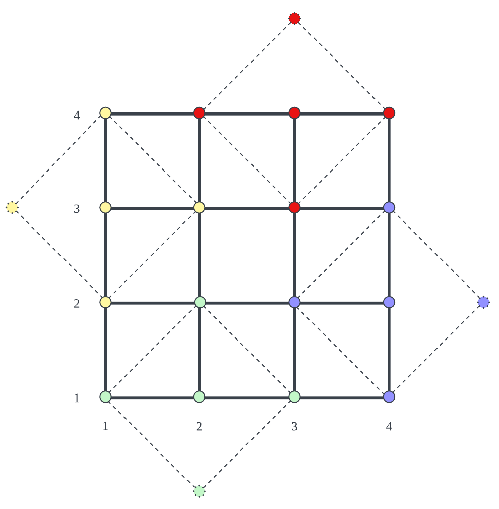
Figure 3: A four-by-four grid with rows and columns indexed and the intersection is labeled with its coordinates. $\gamma(\mathcal{G})=4$ and one corresponding dominating set is $\{1-3,2-1,3-4,4-2\}$. The regions constructed based on this set are $\{I_{1-3},I_{2-1},I_{3-4},I_{4-2}\}$.

Our partitioning rule considers the adjacency of intersections and we assume each intersection has at most four adjacent intersections. However, not all regions can contain one center and four leaves. For example, if two centers are adjacent to each other or the center is at the boundary of the grid, then regions constructed based on these centers have less than four leaves. To ensure the completeness of regions, we introduce the fictitious intersection to fill the absence of adjacent intersections and the fictitious intersections will be further handled carefully in the following sections. One region configuration in the $4\times 4$ grid traffic network, where centers are at the boundary, is illustrated in Fig. 3.

IV-D RL Formulation of Regional Agents

In MG, agents interact with environments and learn within multiple episodes. In a complete episode with a length of $\mathcal{T}$ time steps, an agent observes the environment and makes actions at a certain time step $t$. Then the agent receives the reward and the observation of the next time step.

IV-D1 Observation Representation

The observation of an agent $i$ whose region is $I_{v}$ is a concatenation of all intersections’ states in the region. Formally,

$$o^{t}_{i}=\{s^{t}_{u}\}_{u\in I_{v}}$$ (16)

There are lots of types of state representations $s_{u}$ in literature such as queue length, waiting time and delay[41, 55, 39]. In [40], vehicle wave on each lane is justified with the ability to fully describe the system while the most commonly used state representation is the queue length on each lane. In this paper, we combine the state representation in [56, 33] with the signal phase. Formally,

$$s_{u}^{t}=\{\{wait^{t}[l]\}_{l\in Lane[u]},\{wave^{t}[l]\}_{l\in Lane[u]},phase^{t}[u]\}$$ (17)

The state of a fictitious intersection is a vector of zeros.

IV-D2 Joint Action Space

As defined in Fig. 1, each intersection has four phases. In TSC, two common settings of action for one intersection are ”Switch” or ”Choose Phase”. In the ”Switch” setting, one intersection chooses whether to switch to the next predefined phase or to hold the current phase. Therefore, the phase sequence $P=\{p_{1},p_{2},..\}$ in this setting follows fixed order and only starting time steps are allowed to deviate. In the ”Choose Phase” setting, one intersection chooses which exact phase to run in the next time period. Therefore, both phase sequence and starting time steps vary and this setting offers more flexibility. Moreover, the phase sequence in ”Switch” setting is a subset of that in the ”Choose Phase” setting. To both improve the travel efficiency and demonstrate the strength of our model in high-dimensional action space, the joint action space of a regional agent $i$ is represented as

$$\mathcal{A}_{i}=\{NS,NSL,EW,EWL\}^{|I_{v}|}$$ (18)

IV-D3 Reward Design

The goal of TSC is to improve traffic conditions in a network such as reducing average travel time. However, average travel time can be calculated only after vehicles complete their travel. Therefore, such delayed measurement is not appropriate to be the immediate reward of agents. In [57], for a single intersection, using the queue length as the reward is equivalent to minimizing average travel time. Similar to [36], we assume the reward of a region is the summation of the rewards of its intersections. Regional agents learn to minimize the waiting queue length of all intersections in the region, i.e.,

$$R^{t}_{i}=\sum_{u\in I_{v}}r^{t}_{u}$$ (19)

where the reward of a single intersection $u$ at time step $t$ is defined as

$$r_{u}^{t}=-\sum_{l\in Lane[u]}wait^{t}[l]$$ (20)

IV-E Adaptive-BDQ in Regional Signal Control

In a region of $|I_{v}|$ intersections, there are $|I_{v}|$ action branches and each branch corresponds to one particular intersection. Here, we define that, if the corresponding intersection of one action branch is fictitious, then this action branch is idle. Otherwise, this action branch is activated. In Fig. 3, the fictitious intersections out of the boundary can be modeled as source or sink, and actions on such intersections have no influence on the dynamics inside the region.

However, the original Equation 5 for computing target value using an average of all branches may mislead the estimate of the target value and further limit the performance of agents. Therefore, we propose Adaptive-BDQ (ABDQ) in which the computation of target values in Eq. (5) is further modified. For agent $i$, the Q-value of intersection $k$ and action $a_{i,k}$ at time step $t$ is $Q_{i,k}(o^{t}_{i},a_{i,k})$. Instead of calculating the average of all branches $k$, the Q-value of the next state is the average of activated action branches $\tilde{k}$, i.e.,

$$y_{\tilde{k}}=r+\gamma\frac{1}{\tilde{N}}\sum_{\tilde{k}}Q^{-}_{\tilde{k}}(o_{i}^{t+1},\underset{a^{\prime}_{\tilde{k}}\in\mathcal{A}_{\tilde{k}}}{\text{arg max}}Q_{\tilde{k}}(o_{i}^{t+1},a_{\tilde{k}}^{\prime}))$$ (21)

where $\tilde{N}$ is the number of activated action branches. In the loss function, only errors of activated branches are involved:

$$L=\mathbb{E}_{(o,a,r,o^{\prime})\sim D}[\frac{1}{\tilde{N}}\sum_{\tilde{k}}(y_{\tilde{k}}-Q_{\tilde{k}}(o,a_{\tilde{k}})^{2}]$$ (22)

IV-F Components and Pipeline of Training Framework

In RL, there are two major components– Environment and agent. Agent receives observations from the environment and returns actions. The environment then moves to the next step and passes transition tuples and the next observation to agents. The architecture of our training is illustrated in Fig. 4. Since the state of the simulator needs further augmented into observation, a Pipeline class is introduced to process data from the simulator and agents. The procedure of Pipeline is listed in Algorithm 2. As shown in Fig. 3, the position of fictitious intersection varies in different regions. Thus, the indices of idle action branches are different among different regions. To accelerate convergence and improve generalized ability, we adopt the centralized learning but decentralized execution (CLDE) paradigm where agents share network parameters and experience memory.

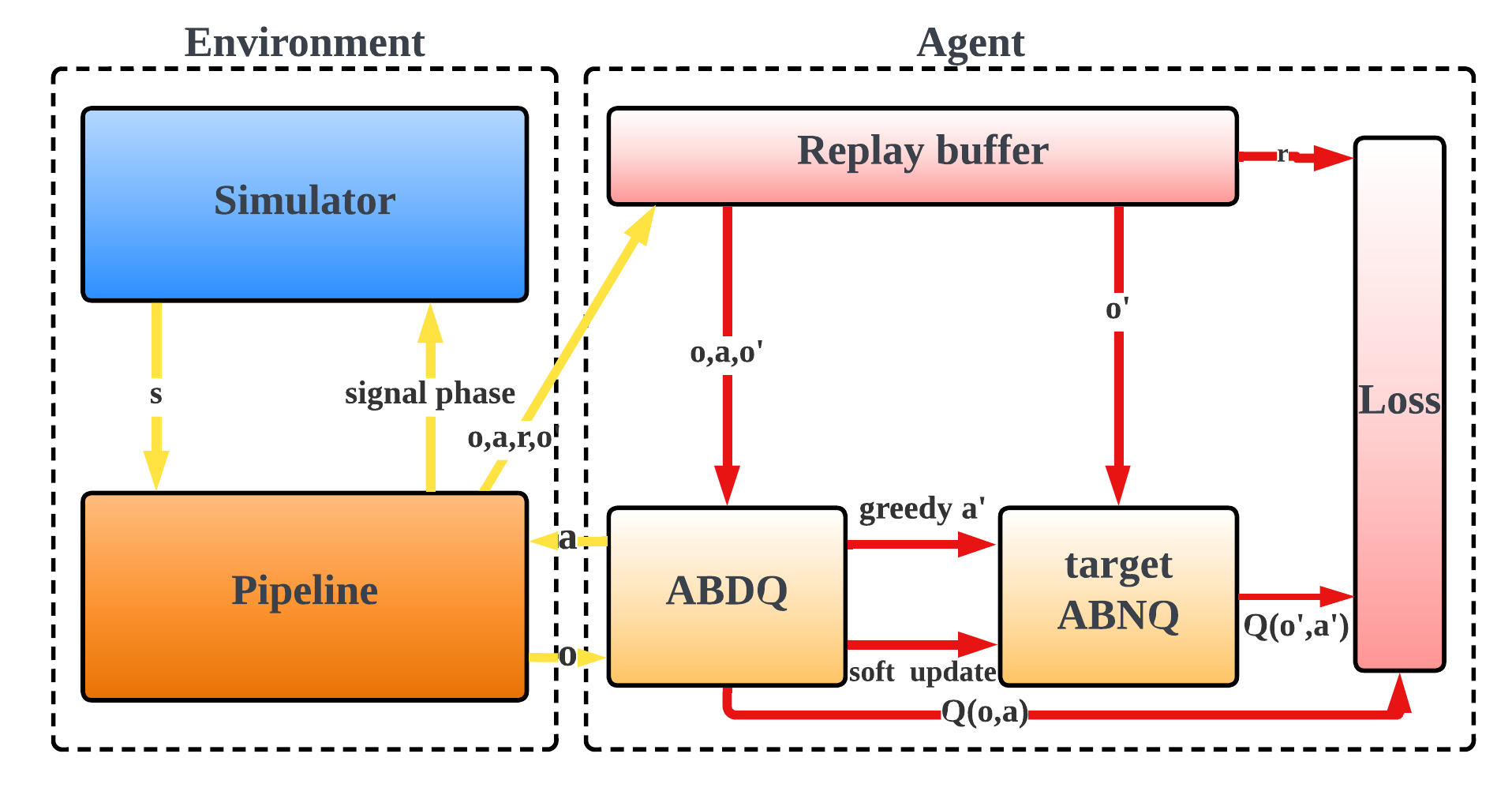
Figure 4: The training framework of RegionLight. Two major components communicate and exchange data through Pipeline Class. The working flow is separated into two parts. The first part is the interaction between the agent and the environment (Yellow arrows) and the second part is the learning and network updating of the agent (Red arrows). In the simulation step of the interaction part, the simulator passes the state to the pipeline and the pipeline then generates observations for agents. Based on the observation, the agent chooses joint action $a$ under $\epsilon$-greedy policy and passes the joint action to the pipeline. Finally, the pipeline passes signal phases to simulation and moves to the next simulation step.

Algorithm 2 Algorithm for Pipeline

1:Initialise ADBQ $\theta_{i}$ and target ADBQ $\theta^{-}_{i}\leftarrow\theta_{i}$

2:Initialise Replay Memory $D_{i}$, Region Configuration $I$

3:while $i<episode$ do

4:     $s\leftarrow$ environment reset

5:     $o_{i}\leftarrow$ generate observation based on $s,I$

6:     while $t<T$ do

7:         if $rand<\epsilon$ then

8:              $a_{i}\leftarrow$ random joint action

9:         else

10:              $a_{i}\leftarrow\cup_{\tilde{d}}\underset{a^{{}^{\prime}}_{\tilde{d}}\in A_{\tilde{d}}}{\text{arg max}}Q_{\tilde{d}}(o_{i},a_{\tilde{d}}^{\prime})$

11:         end if

12:         $r,s^{\prime}\leftarrow$ env step after all agents choose actions

13:         calculate$R_{i}$ and generate $o_{i}^{\prime}$ based on $s^{\prime},I$

14:         store transition$(o_{i},a,R_{i},o_{i}^{\prime})$ to $M_{i}$

15:         Update $\theta$ by Eq. (6) with target value by Eq. (21)

16:         $\theta_{i}^{-}\leftarrow(1-\tau)\theta_{i}^{-}+\tau\theta_{i}$ for certain step

17:         $o_{i}\leftarrow o_{i}^{\prime}$

18:     end while

19:end while

V Experiments and Results

In this section, we test our method in both real and synthetic grids and compare it with other novel MADRL frameworks. To show the robustness of our region design, two different minimum dominating sets are used to construct region configurations in two $4\times 4$ grid networks, and different shuffled assignment orders are applied in the $16\times 3$ grid network. To evaluate the improvement of ABDQ in controlling partially loaded regions, we test ABDQ on minimum-dominating-set-based regions which contain one fictitious intersection, and $2\times 3$ regions which contain two fictitious intersections.

V-A Experiment Scenario

The traffic simulator CityFlow we used in this paper is an open-source simulator [58]. In our experiment, one real $4\times 4$ grid (Hangzhou), one synthetic $4\times 4$ grid and one real $16\times 3$ grid (Manhattan) are used. Roadnets of Hangzhou and Manhattan are illustrated in Fig. 5.

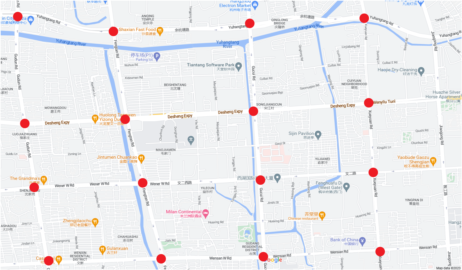
(a) Gudang, Hangzhou

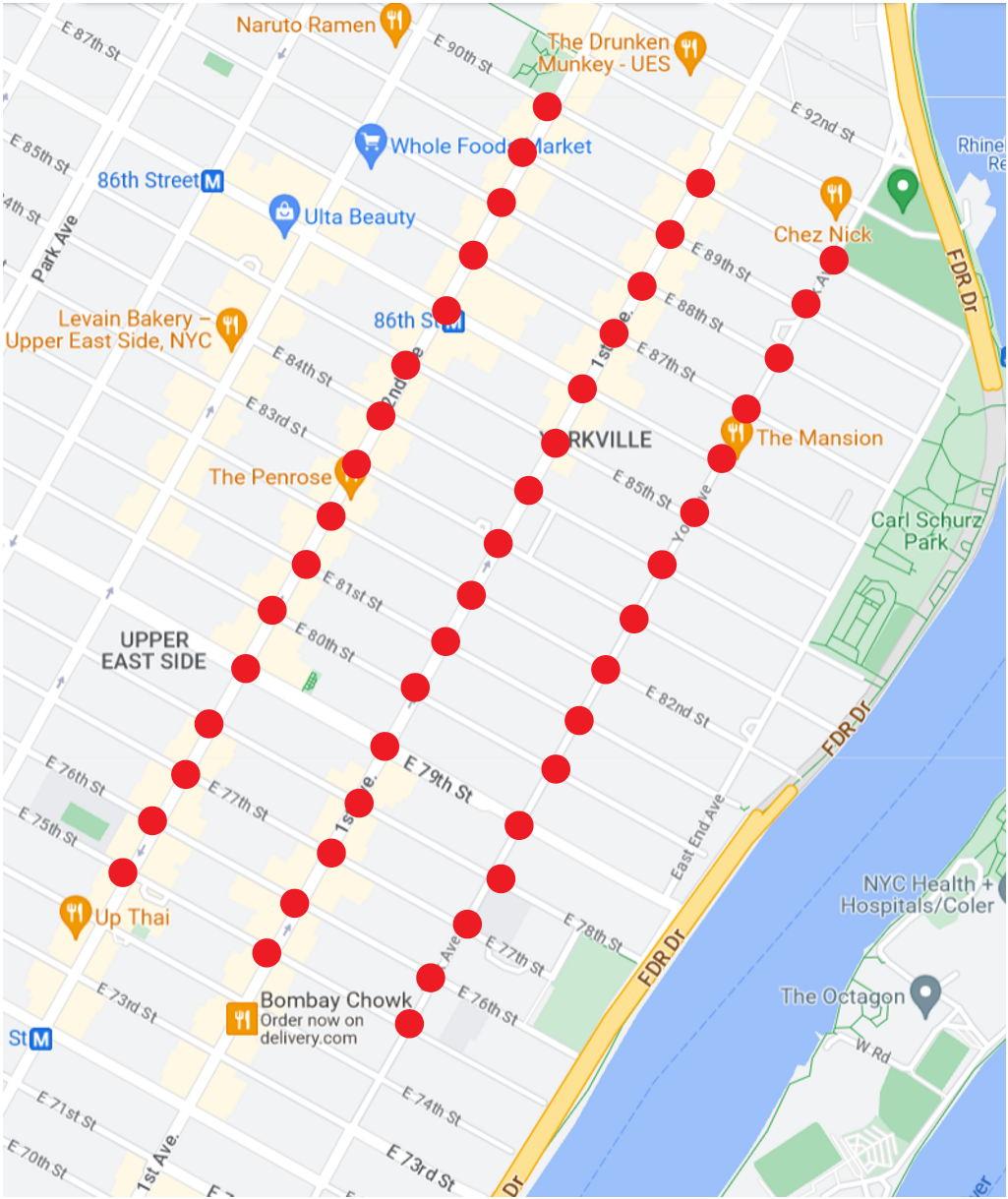
(b) Manhattan

Figure 5: Road networks for Hangzhou and Manhattan Grid. Traffic signals controlled by agents are marked with red dots.

In the Hangzhou network, two traffic flows, whose volumes are derived from camera data, are used, i.e., one is in flat hours and the other is in peak hours. The turning ratio for both flat and peak flows is synthesized from the statistics of taxi GPS data. In the synthetic network, the flow is generated according to Gaussian distribution, and the turning ratio for synthetic flow is distributed as 10% (left turn), 60% (straight), and 30% (right turn). In the Manhattan network, the flow is sampled from taxi trajectory data and the turning ratios of each movement at different intersections are not identical. The statistics of flows and the distance between neighboring intersections are listed in Table II. All these datasets are open-sourced.

TABLE II: Flow and Network statistics

Scenario	Arrival Rate(vehicles/s)		Distance
	Mean	Std
(Hangzhou) Flat	0.83	1.33	600m
(Hangzhou) Peak	1.82	2.15	600m
Synthetic-1	3.12	4.08	300m
Synthetic-2	3.12	4.08	600m
Manhattan	0.78	2.49	100m (NS), 350m (EW)

The length of each episode is set to 4000s. To avoid signals flicking too frequently, all agents perform actions for every $\Delta t=$10s and no yellow phase is inserted between different phases. Then, the length $\mathcal{T}$ of one episode is 400.

We compare our agent with both non-RL and RL baselines. Non-RL baselines include Fixed time, Max Pressure, SOTL, Genetic Algorithm and Artificial Bee Colony. RL baselines include NeighbourRL, R-DRL, CoLight, PNC-HDQN and ENC-HDQN. For ABDQ, the neural network structure follows the BDQ [51] and is illustrated in Fig. 2. The size of hidden layers of NeighbourRL is the same as ABDQ. For R-DRL, the structures of actor and critic follow the description in [36]. Although a global critic is proposed to coordinate R-DRL, the convergence of this global critic is not guaranteed. So only R-DRL agents are compared. The hyperparameters for our agent, NeighbourRL and R-DRL are listed in Table IV.

For other baselines, we run the source code for fairness.The proposed framework is open-sourced and is coded in Python. Gurobi, a third-party Python package, was used to formulate and solve the linear integer programming problem[59]. The RL agent was coded with Tensorflow developed by Google[60].

V-B Metric

TABLE III: Numerical Statistics for non-RL Baselines

Flow	Metric	Fixed	Max Pressure	SOTL	Genetic	Artificial	RegionLight(OURS)	RegionLight(OURS)
					Algorithm	Bee Colony	$\gamma=0.9$	$\gamma=0.99$
Flat	ATT	482.19	434.65	364.42	399.91	345.10	319.14$\pm$0.43	319.28$\pm$0.43
	AQL	0.57	0.52	0.25	0.34	0.16	0.07$\pm$0.0016	0.07$\pm$0.0017
	TP	2810	2854	2919	2923	2942	2963.27$\pm$0.89	2963.75$\pm$0.88
Peak	ATT	803.78	525	435.72	574.2	567.87	402.02$\pm$3.00	402.93$\pm$3.27
	AQL	1.8	1.42	0.82	1.45	0.95	0.44$\pm$0.01	0.45$\pm$0.01
	TP	5105	6176	6224	6046	5926	6382.19$\pm$10.9	6385.8$\pm$11.26
Synthetic-1	ATT	548.77	235.29	284.47	-	531.55	206.6$\pm$1.3	207.60$\pm$1.2
	AQL	3.32	1.19	1.78	-	3.22	0.85$\pm$0.016	0.86$\pm$0.013
	TP	9553	11181	11166	-	9648	11227.93$\pm$1.07	11227.056$\pm$0.94
Synthetic-2	ATT	685.63	474.64	454.74	557.32	519.01	381.38$\pm$ 1.20	382.82$\pm$1.26
	AQL	4.65	2.15	1.76	3.02	2.81	0.85$\pm$ 0.015	0.87$\pm$0.016
	TP	9218	10690	10810	10094	10146	11033.78$\pm$8.75	11029.40$\pm$10.76
Manhattan	ATT	1198.24	287.62	340.67	-	-	176.46$\pm$0.316	177.75$\pm$0.415
	AQL	1.09	0.13	0.21	-	-	0.024$\pm$0.0004	0.025$\pm$0.0004
	TP	1116	2799	2754	-	-	2824$\pm$0.0	2824$\pm$0.0

TABLE IV: Hyperparameter Summary

Component	Hyperparameter	Value
ABDQ	$\gamma$	0.9 & 0.99
	Learning rate $\alpha$	0.0001
	Replay Buffer Size	200000
	Network optimizer	Adam
	Activation Function	Relu
	$\tau$	0.001
	Batch Size	32
R-DRL	$k$	128 (4$\times$ 4), 1024 (16$\times$ 3)
	$\alpha_{\text{critic}}$	0.0001
	$\alpha_{\text{actor}}$	0.00001
$\epsilon$-greedy Policy	$\epsilon_{max}$	1
	$\epsilon_{min}$	0.001
	decay steps	20000

Similar to [32], we choose three metrics to evaluate the performance of agents.

• Average Travel Time (ATT): average of all vehicles’ travel time. Since the time step of our simulation is larger than the arrival time span, all vehicles can travel in the network for enough time and the computation of ATT is more complete and less affected by vehicles which just depart;

• Average Queue Length (AQL): average queue length on each lane of all intersections. The definition of the reward of our agent is the sum of queue length. So AQL is a direct numerical interpretation of reward;

• Throughput (TP): number of vehicles that arrive at the destination. While reducing ATT, we also want to increase TP so that benefits are maximized.

V-C Overall Performance

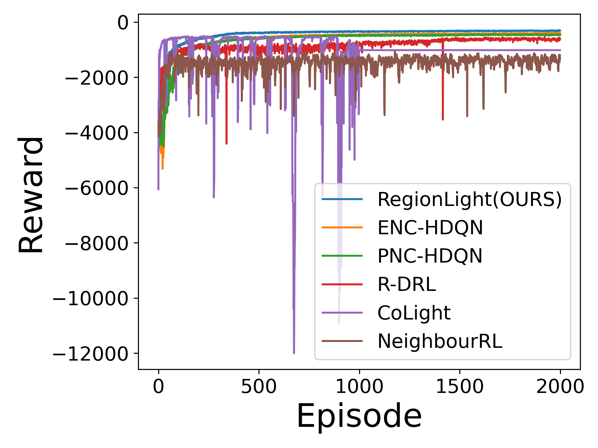
(a) (Hangzhou)Flat

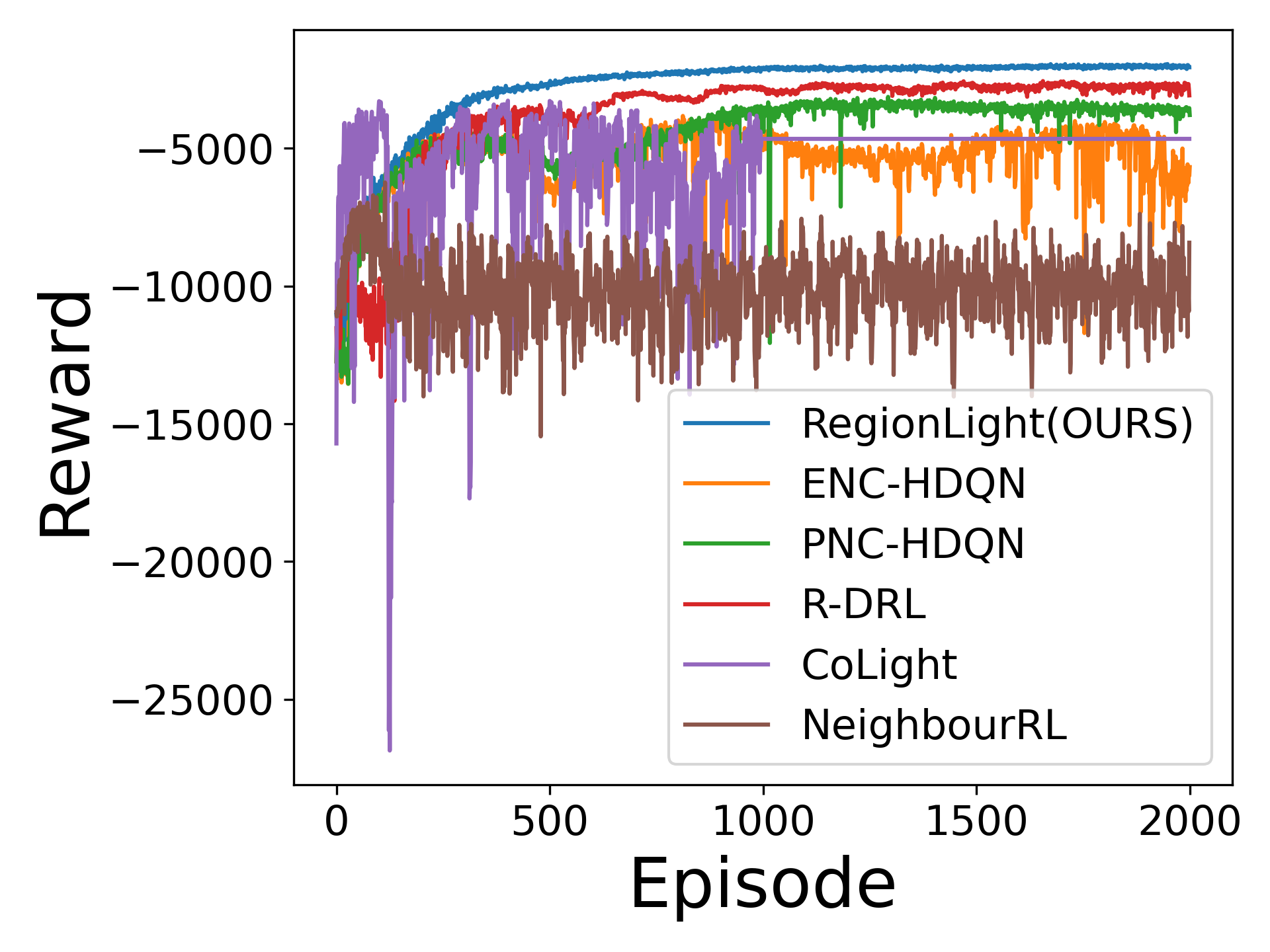
(b) (Hangzhou)Peak

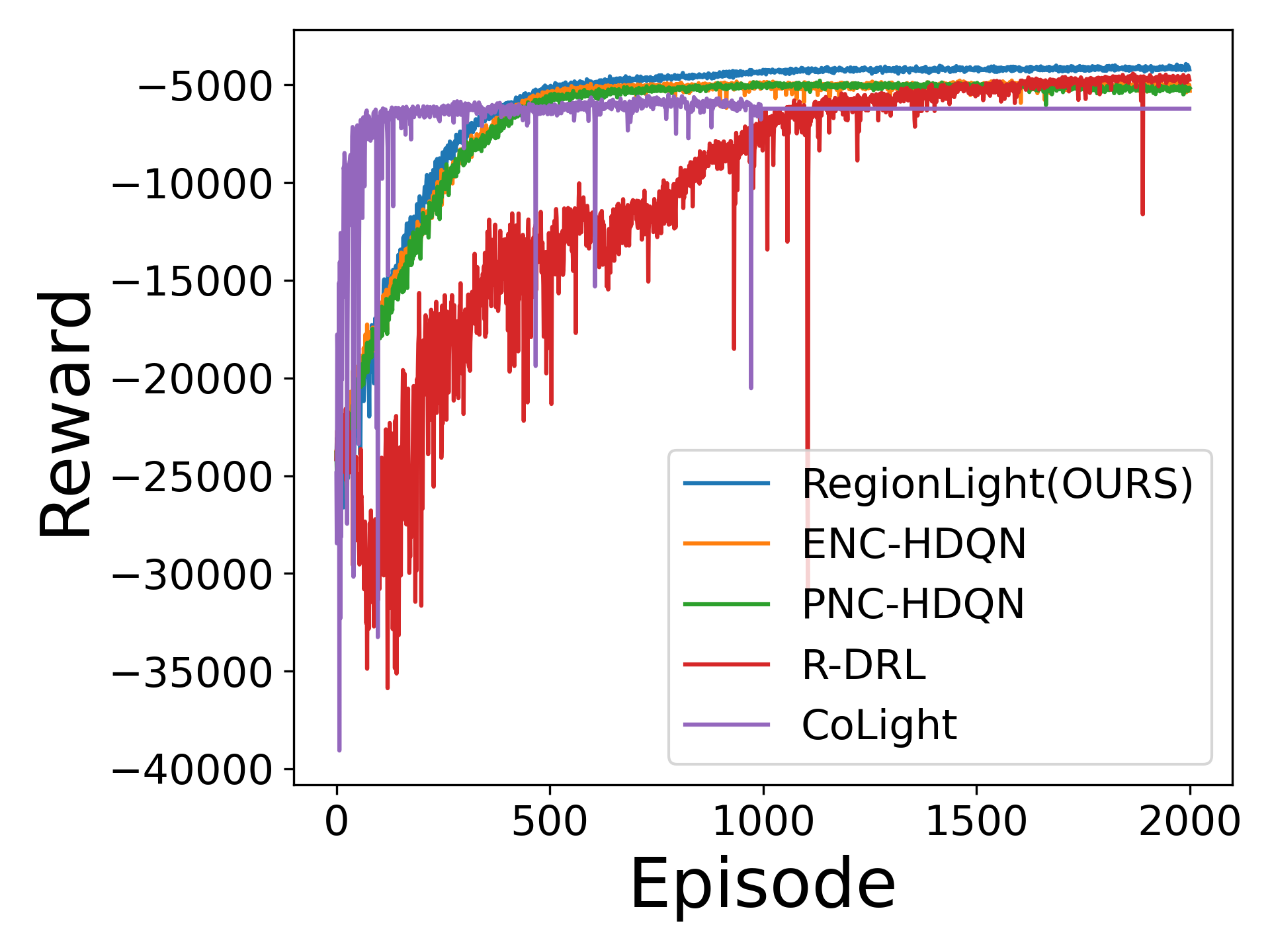
(c) Synthetic-1

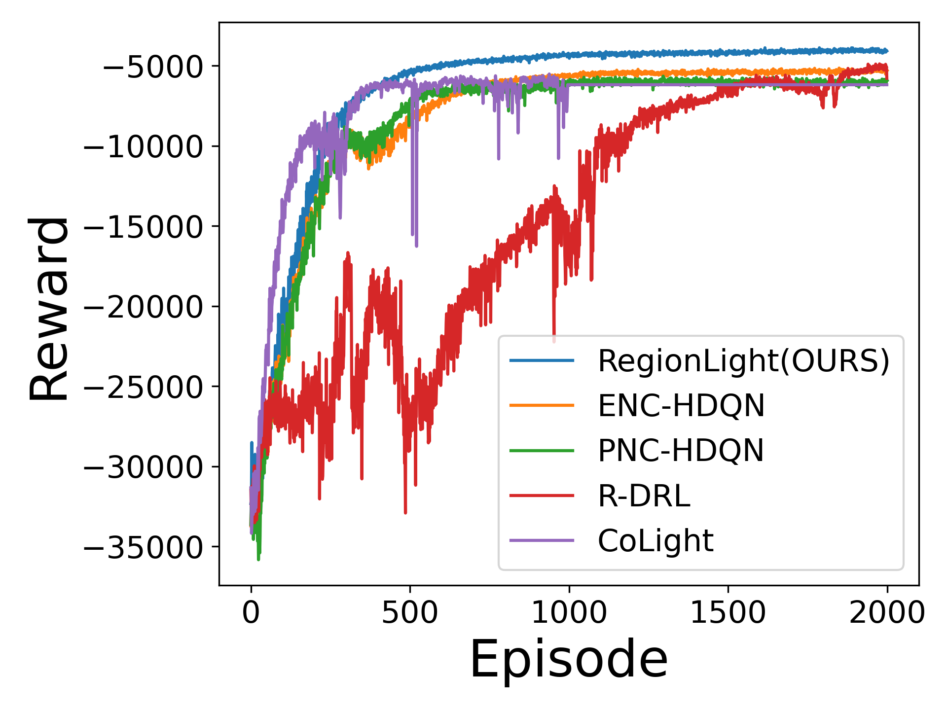
(d) Synthetic-2

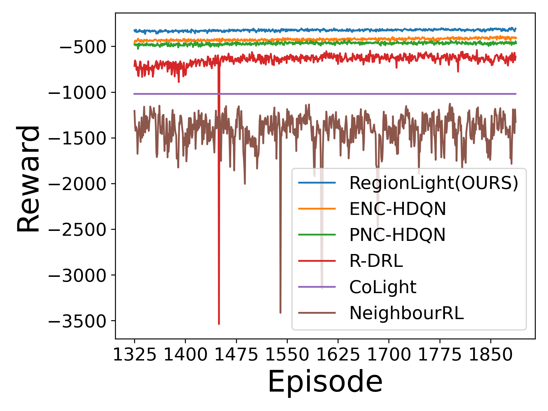
(e) Flat after Convergence

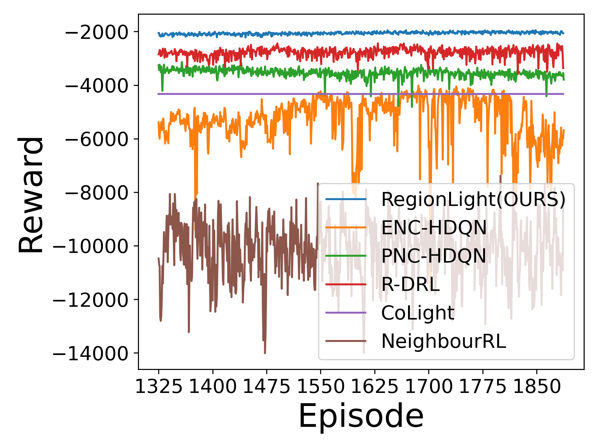
(f) Peak after Convergence

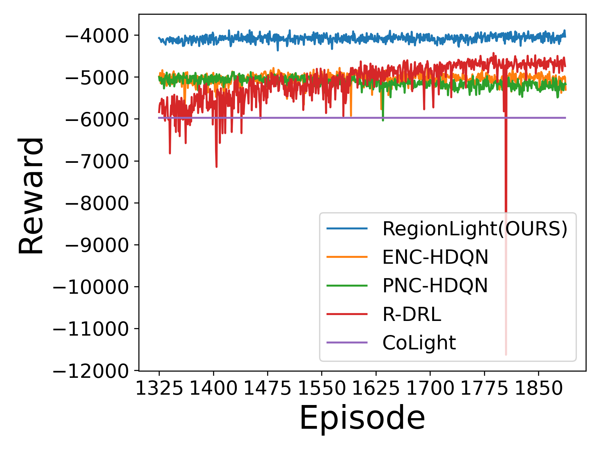
(g) Synthetic-1 after Convergence

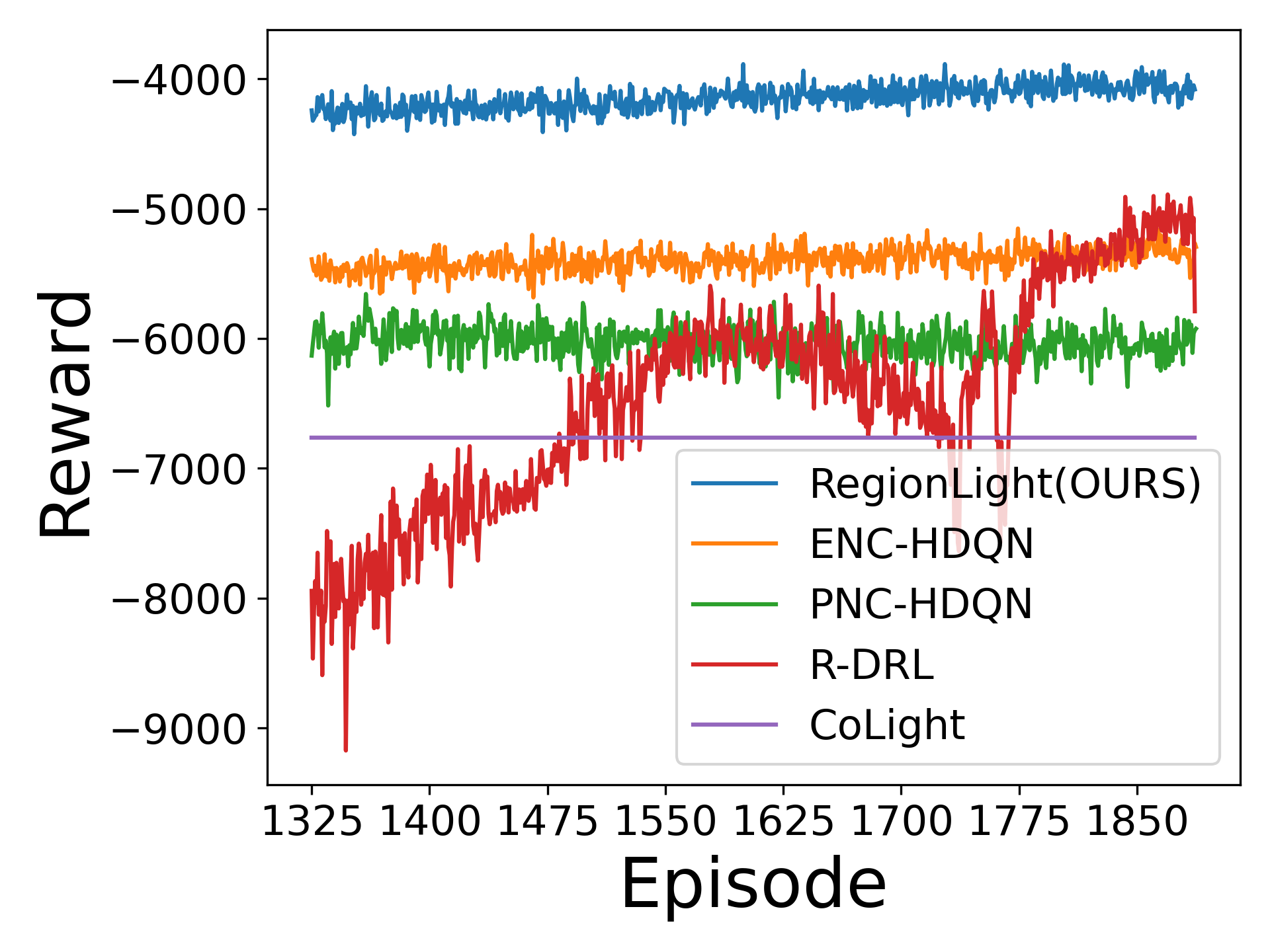
(h) Synthetic-2 after Convergence

Figure 6: Learning curve of RL agents in $4\times 4$ networks. The top three pictures are the overall performance during 2000 episodes and the bottom three pictures are the overall performance after episode 1250. Curves of methods failing to converge are omitted.

(a) Manhattan

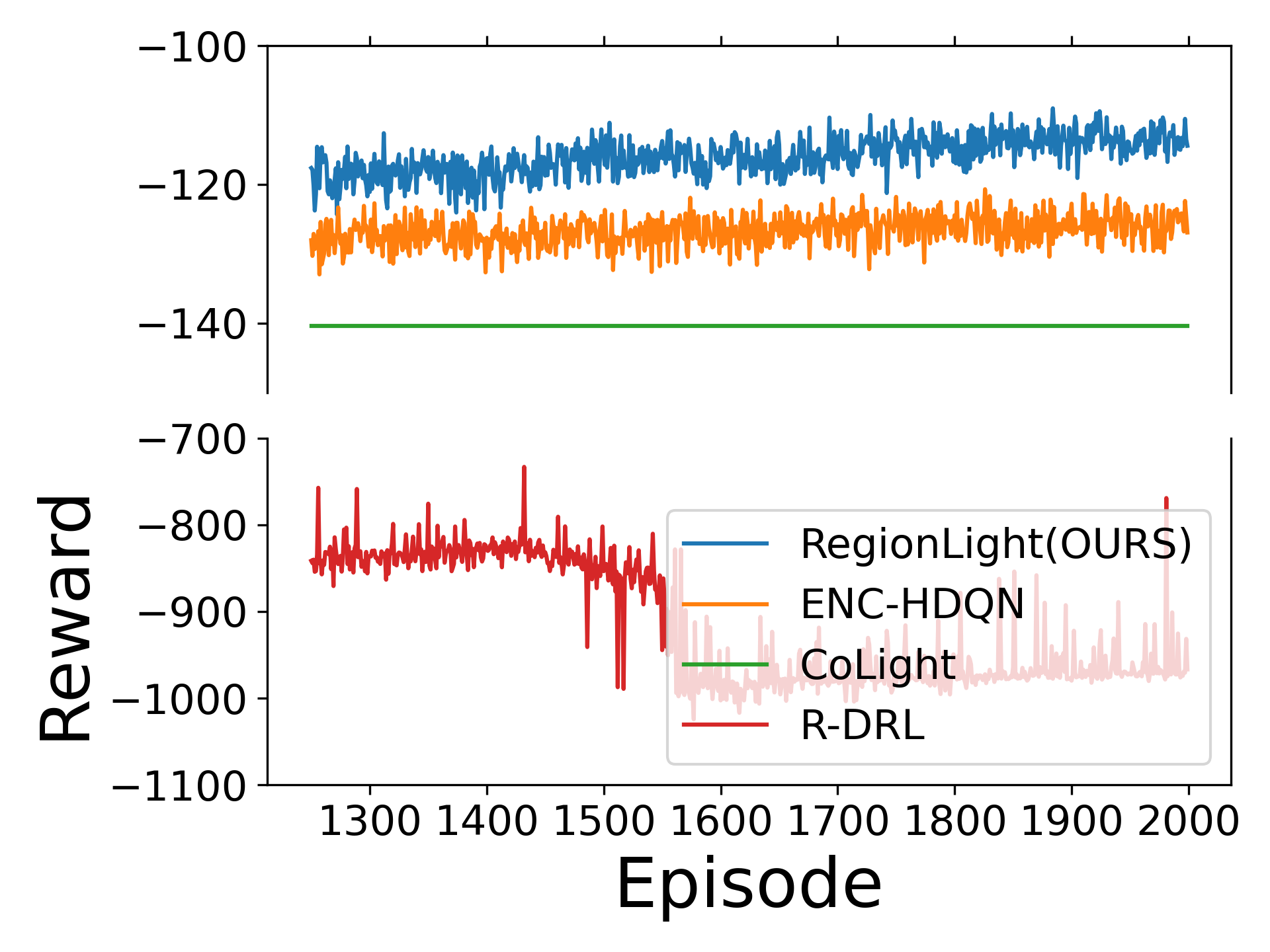
(b) Manhattan after Convergence

Figure 7: Learning curve of RL agents in $16\times 3$ networks. The left picture is the overall performance during 2000 episodes and the right picture is the overall performance after episode 1250. Curves of methods failing to converge are omitted.

TABLE V: Numerical Statistics for RL Baselines

Flow	Metric	NeighbourRL	R-DRL	CoLight	PNC-HDQN	ENC-HDQN	RegionLight	RegionLight
							(OURS)	(OURS)
							$\gamma=0.9$	$\gamma=0.99$
Flat	ATT	379.83$\pm$8.37	335.29$\pm$1.65	334.01$\pm$0.95	328.13$\pm$0.49	326.23$\pm$0.59	319.14$\pm$0.43	319.28$\pm$0.43
	AQL	0.29$\pm$0.031	0.13$\pm$0.01	0.28$\pm$0.34	0.10$\pm$0.0020	0.09$\pm$0.0021	0.07$\pm$0.0016	0.07$\pm$0.0017
	TP	2930.79$\pm$7.19	2950.75$\pm$3.81	2899.92$\pm$144.7	2942.9$\pm$3.09	2959.776$\pm$1.60	2963.27$\pm$0.89	2963.75$\pm$0.88
Peak	ATT	675.01$\pm$60.26	415.75$\pm$4.94	463$\pm$7.11	437.09$\pm$5.84	479.25$\pm$26.14	402.02$\pm$3.00	402.93$\pm$3.27
	AQL	2.17$\pm$0.21	0.58$\pm$0.04	1.31$\pm$0.37	0.75$\pm$0.03	1.12$\pm$0.23	0.44$\pm$0.01	0.45$\pm$0.01
	TP	5669.4$\pm$226.92	6340.18$\pm$18.28	6034$\pm$370.6	6296.85$\pm$29.96	6222.2$\pm$136.89	6382.19$\pm$10.9	6385.8$\pm$11.26
Synthetic-1	ATT	-	216.03$\pm$7.28	246.14$\pm$18.19	228.24$\pm$2.0	224.6$\pm$1.6	206.6$\pm$1.3	207.60$\pm$1.2
	AQL	-	0.99$\pm$0.1	1.27$\pm$0.2	1.08$\pm$0.02	1.05$\pm$0.02	0.85$\pm$0.016	0.86$\pm$0.013
	TP	-	11173.29$\pm$63.63	11179.2$\pm$201.3	11179.8$\pm$15.67	11215.41$\pm$4.96	11227.93$\pm$1.07	11227.056$\pm$0.94
Synthetic-2	ATT	-	411.33$\pm$9.64	422$\pm$12.9	415.42$\pm$1.91	404.82$\pm$1.39	381.38$\pm$1.20	382.82$\pm$1.26
	AQL	-	1.3$\pm$0.3	1.27$\pm$0.06	1.26$\pm$0.023	1.11$\pm$0.016	0.85$\pm$0.015	0.87$\pm$0.016
	TP	-	10919.38$\pm$83.08	10896.47$\pm$33.66	10886.39$\pm$15.45	10965.65$\pm$9.81	11033.78$\pm$8.75	11029.40$\pm$10.76
Manhattan	ATT	-	319.82$\pm$4.34	184.25$\pm$2.437	-	181.25$\pm$0.372	176.46$\pm$0.316	177.75 $\pm$0.415
	AQL	-	0.2$\pm$0.005	0.047$\pm$0.0024	-	0.026$\pm$0.0005	0.024$\pm$0.0004	0.025$\pm$0.0004
	TP	-	2597.12$\pm$7.81	2824$\pm$0.0	-	2823.996$\pm$0.063	2824$\pm$0.0	2824$\pm$0.0

We first compare our model with non-RL baselines. Numerical statistics results are listed in Table III. The results of the Artificial Bee Colony in Manhattan scenarios and those of the genetic algorithm in Synthetic-1 and Manhattan scenarios are omitted because these algorithms failed to converge after random initialization. From Table III, we can observe that our model outperforms other baselines in all metrics

Then we compare our model with RL baselines. Since the definitions of the reward of RL baselines involve augmentations, we computed the episode reward as the below equation for consistency, i.e.,

$$R=\frac{1}{|\mathcal{V}|}\sum_{t=1}^{\mathcal{T}}\sum_{v}r_{v}^{t}$$ (23)

The learning process of RL models involves lots of episodes. Therefore, we plot the learning curve of episode reward of all RL baselines. Since NeighbourRL failed to converge in the Synthetic and Manhattan datasets and PNC-HDQN failed to converge in the Manhattan dataset, the corresponding curves are omitted. Meanwhile, the performance of our model under different parameter sets is almost identical. Therefore, we only plot the learning curve of our model under $\gamma=0.9$. As illustrated in Fig. 6 and 7, our agent converges in all scenarios. As the arrival rate increases, the curve becomes oscillated. However, our agent is the most stable one and with the smallest fluctuation. From the bottom plots in Fig. 6, our agent achieves the highest reward after convergence.

Numerical results are listed in Table V and III where the results of models that fail to converge are omitted. We first look at $4\times 4$ networks, i.e., Hangzhou(Flat), Hangzhou(Peak), Synthetic-1 and Synthetic-2. In the Hangzhou scenario, as the flow density increases, the average travel time becomes longer and the network becomes congested. In two synthetic scenarios, the only difference is the distance between two intersections. Therefore, vehicles travels longer distances and the average travel time is much longer. Moreover, the throughput of Synthetic-2 is slightly smaller than that of Synthetic-1 because, in Synthetic-2, the remaining time is not enough for those vehicles which depart near the end of episode. The average queue length of regional agents in the both synthetic scenarios almost doubles that in the Hangzhou peak scenario while those of CoLight and ENC even decrease. This is probably caused by two factors: The first is the distance between intersections and the arrival rate; If intersections are close, the travel time between intersections becomes much shorter and it is harder to decrease the queue length. The second is that regional agents try to minimize the total queue length in a region and some intersections may have to sacrifice individual rewards to achieve better regional rewards. In the Manhattan scenario, some baselines fail to converge probably due to more complex traffic dynamics in the huge network even though the flow of Manhattan is not as demanding as Hangzhou scenarios. The difference in throughput between agents is not significant because simulation steps are large enough for most vehicles to arrive at their destinations. Overall, our agent achieves the best results and the smallest standard deviation among all metrics.

V-D Robustness of Our Region

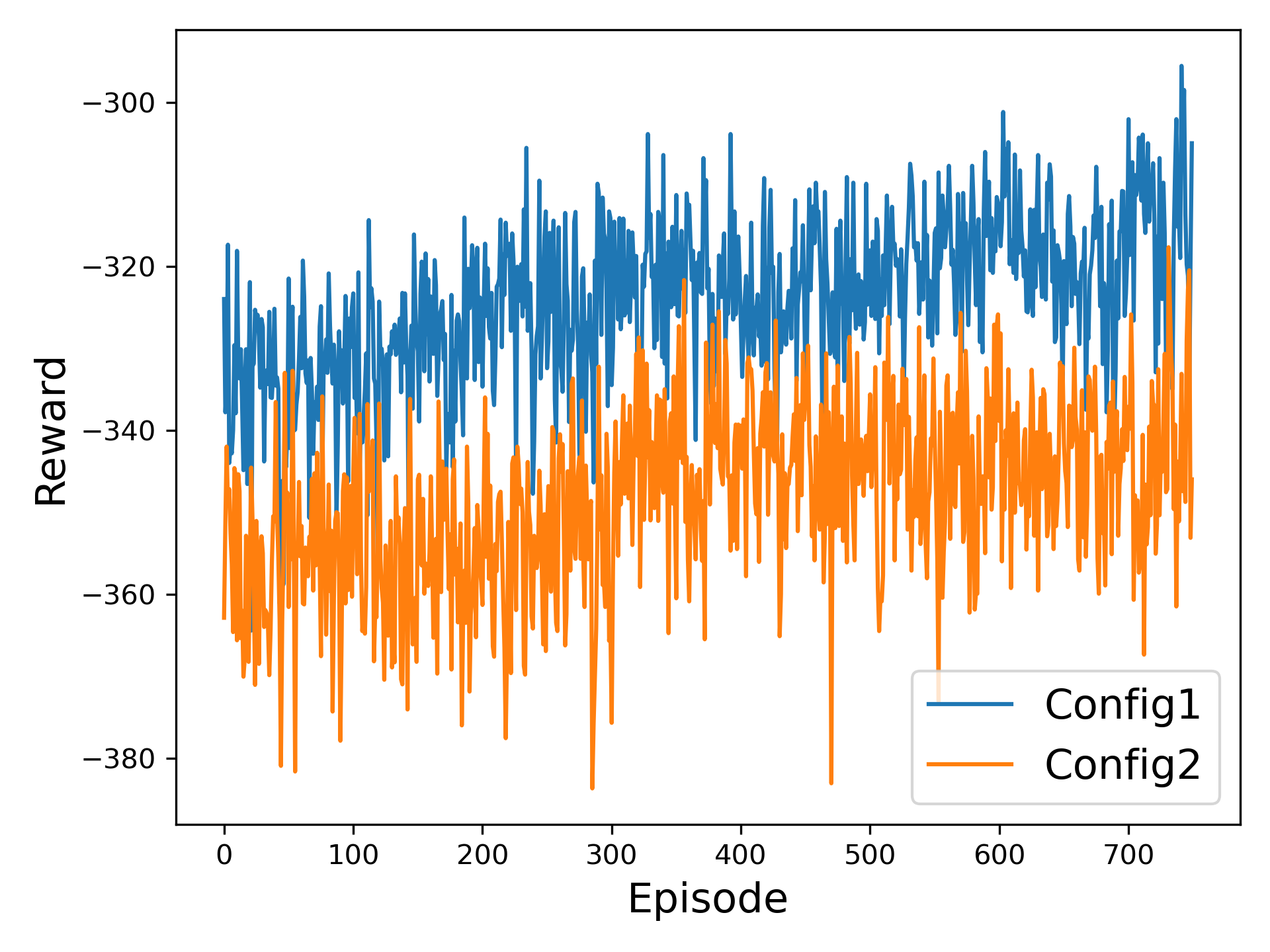
(a) (Hangzhou)Flat

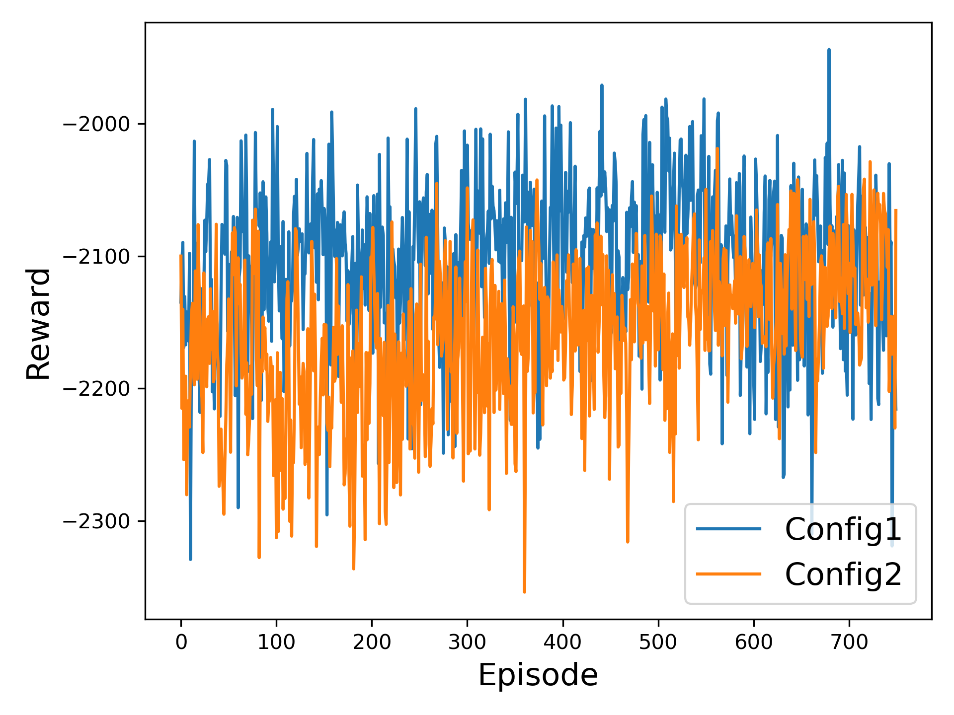
(b) (Hangzhou)Peak

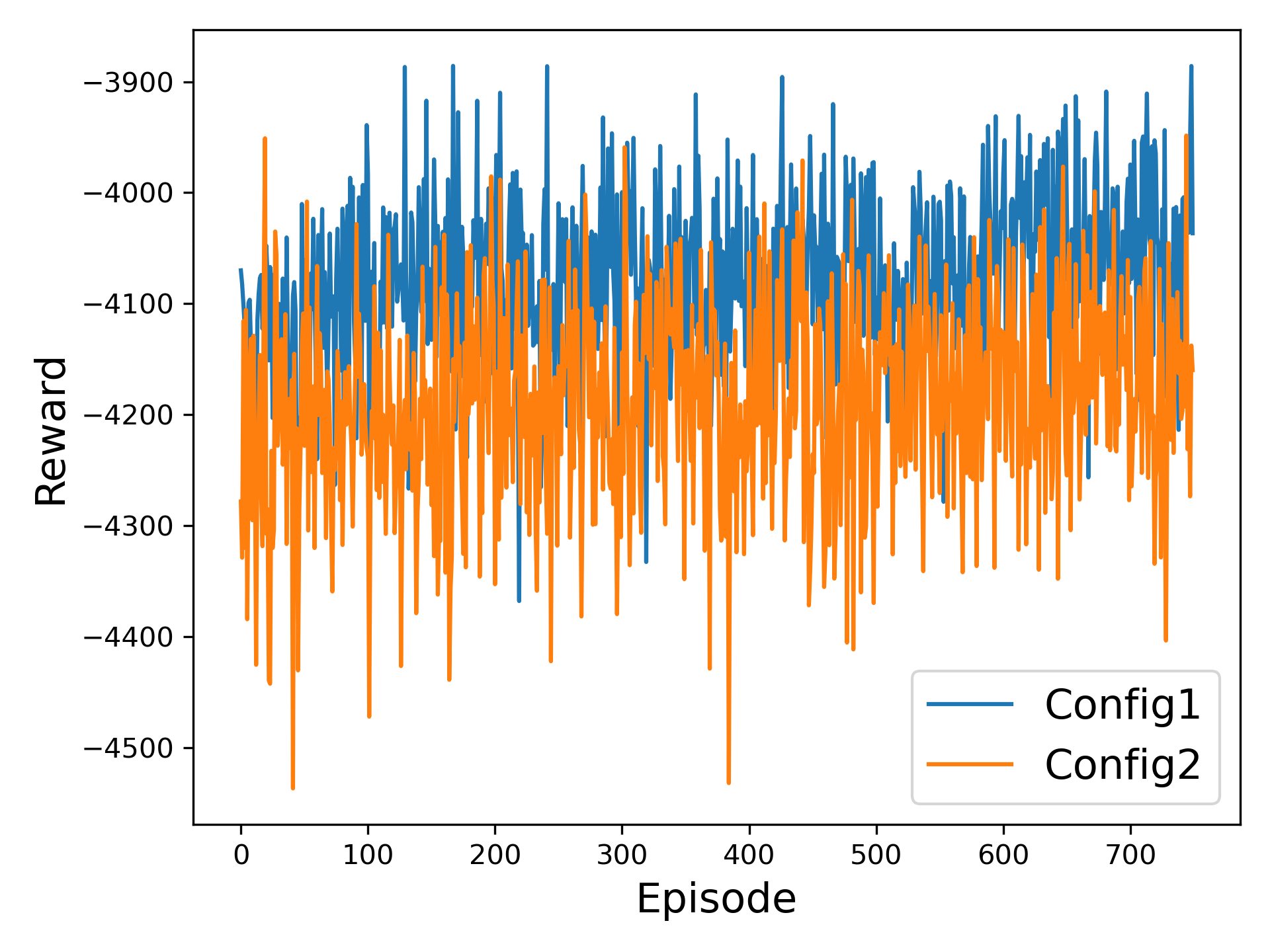
(c) Synthetic-1

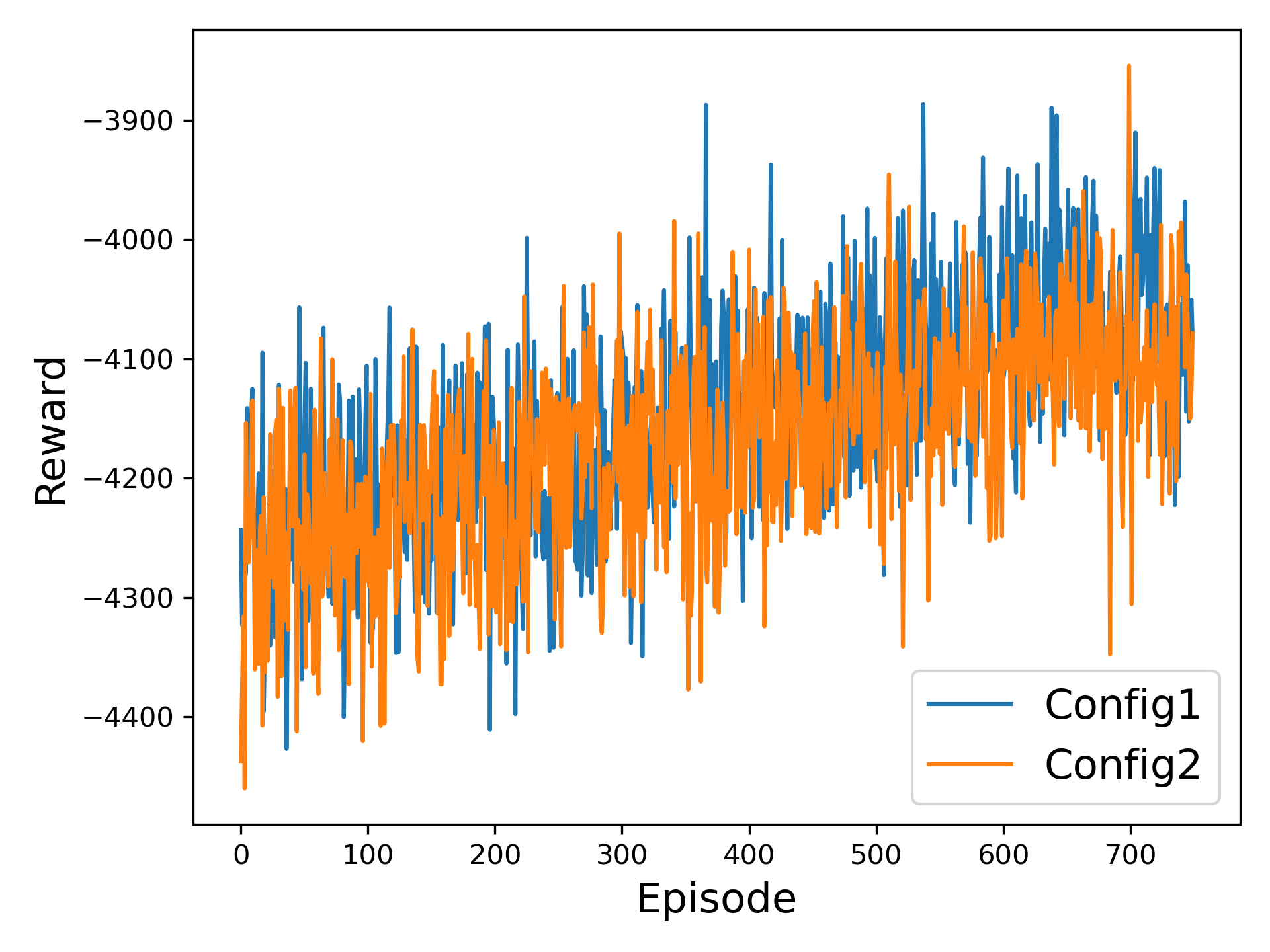
(d) Synthetic-2

Figure 8: Learning curves of two region configurations in $4\times 4$ grid.

As illustrated in Fig. 3, we generate the unique region configuration based on one minimum dominating set and only one intersection in the region is fictitious. However, one graph may have different minimum dominating sets which generate new sets of region configuration. For the $4\times 4$ grid network, there are two minimum dominating sets. The region configuration generated by first minimum dominating set is $I_{1-3},I_{2-1},I_{3-4},I_{4-2}$ (Config1) in Fig. 3. The other unique region configuration under the other minimum dominating set is $I_{1-2},I_{2-4},I_{3-1},I_{4-3}$ (Config2). To ensure the completeness of the experiment, we compare the performance of agents under both configurations. The learning curves are plotted in Fig. 8. Agents under both configurations converge but Config2 has a lower converged performance. These training curves indicate that the configuration of regions can affect the training process of agents. In different configurations, agents observe different sets of intersections and traffic flows of these intersections are different. The numerical results are listed in Table VI. We can observe that there is no significant difference and the numerical results of Config2 are still the best among all baselines.

TABLE VI: Numerical Statistics of Two Configurations

Flow	Metric	Config1	Config2
Flat	ATT	319.14$\pm$0.43	320.62$\pm$0.48
	AQL	0.07$\pm$0.0016	0.07$\pm$0.0019
	TP	2963.27$\pm$0.89	2963.03$\pm$0.81
Peak	ATT	402.02$\pm$3.00	406.99$\pm$4.67
	AQL	0.438$\pm$0.01	0.443$\pm$0.009
	TP	6382.19$\pm$10.9	6369.724$\pm$15.2
Synthetic-1	ATT	206.6$\pm$1.3	208.27$\pm$1.27
	AQL	0.85$\pm$0.0157	0.86$\pm$0.0162
	TP	11227.93$\pm$1.07	11227.41$\pm$ 1.34
Synthetic-2	ATT	381.38$\pm$1.20	381.80$\pm$1.2
	AQL	0.85$\pm$0.015	0.86$\pm$0.015
	TP	11033.78$\pm$8.75	11030.73$\pm$8.84

If the minimum dominant set does not meet Theorem 1, then different iteration orders of line 13 in Algorithm 1 can construct different sets of region configuration according to Remark 2. We tried several assignment orders to investigate whether different assignment orders could affect performance. From Table VI, even for configurations constructed from different minimum dominating sets, the performance of models under those configurations is very close. Therefore, we listed the results of worst performance, average performance, and best performance after convergence. From Table VII, numerical statistics indicate that, although performance under different assignment orders is not identical, the difference is very close and performance is consistent.

TABLE VII: Numerical Statistics of Different Assignment Orders in Manhattan Scenario

	ATT	AQL	TP
Best Performance	176.03$\pm$0.501	0.0241$\pm$0.0412	2824$\pm$0.0
Average Performance	177.64$\pm$0.684	0.0245$\pm$0.0415	2824$\pm$0.0
Worst Performance	178.25$\pm$0.641	0.0249$\pm$0.0419	2824$\pm$0.0

V-E Improvement of ABDQ over BDQ and DDPG+WA

The computation of target values in ABDQ only involves activated branches to relieve the negative influence of fictitious intersections.

TABLE VIII: Improvement by ABDQ

Flow	Metric	Config1	$2\times 3$ Grid
Flat	ATT	2.8%	3.5%
	AQL	9.7%	24.1%
	TP	0.14%	0.27%
Peak	ATT	1.1%	1.8%
	AQL	7.8%	19.3%
	TP	0.12%	0.42%
Synthetic-1	ATT	1.7%	2.4 %
	AQL	8.5%	11.8%
	TP	0.27%	0.34%
Synthetic-2	ATT	2.3%	5.2%
	AQL	9.4%	18.9%
	TP	0.35%	1.3%

To show the advantage of ABDQ, we applied BDQ on ”Config1” and ABDQ on $2\times 3$ grid regions. ”Config1” has one fictitious intersection and the $2\times 3$ grid region has two fictitious intersections. Both regions have four activated branches in BDQ and ABDQ. In Table VIII, the performance in both region configurations is improved by ABDQ. For different scenarios, the improvement in the Hangzhou flat scenario is more significant than that in other scenarios. For different region configurations, the improvement of the grid region is more significant than ”Config1”. It is probably because there are more fictitious intersections in grid regions and ABDQ alleviates the negative of fictitious intersections effectively.

VI Conclusion and Future Work

In this paper, we proposed a novel regional signal control framework for TSC. Our network partitioning rule has the potential to be applied in non-grid networks because the topology of our region is a star which is composed of one center and an arbitrary number of leaves. Meanwhile, we proposed ABDQ to search for optimal joint action and to mitigate the negative influence of fictitious intersections. There are three major advantages of ABDQ: One is that the search for optimal actions is more efficient because the output size of the neural network grows linearly as the size of the region increases. The second one is intra-regional cooperation control. The last one is that ABDQ mitigates the influence of fictitious intersections by calculating target value and loss based on activated branches.

We have carried out comprehensive experiments to evaluate the performance and robustness of our RL agent. Experiments show that our RL agent achieves the best performance in both real and synthetic scenarios, especially in scenarios with a high-density flow. Also, we observed that the distance between intersections can affect the convergence rate of agents and their performance. Interestingly, different configurations and assignment orders can influence the performance of agents, but the difference is not significant. One limitation of our framework is that we model regional RL agents as independent learners and no explicit cooperation is designed between regions.

In the future, we will focus on the maximum capacity of our region by increasing hops when defining the neighborhood of one intersection. It is also worthwhile to investigate the performance of our model on 8-phases traffic signals and in massive-scale or non-grid traffic networks. Meanwhile, region-wise cooperation is also a promising research direction.

References

- [1] “Inrix 2021 global traffic scorecard: As lockdowns ease uk city centres show signs of return to 2019 levels of congestion,” 2022. [Online]. Available: https://inrix.com/press-releases/2021-traffic-scorecard-uk/
- [2] “Inrix: Americans lost 3.4 billion hours due to congestion in 2021, 42% below pre-covid,” 2022. [Online]. Available: https://inrix.com/press-releases/2021-traffic-scorecard-uk/
- [3] “who releases country estimates on air pollution exposure and health impact_2022,” 2022. [Online]. Available: www.who.int/news/item/27-09-2016-who-releases-country-estimates-on-air-pollution-exposure-and-health-impact
- [4] R. P. Roess, E. S. Prassas, and W. R. McShane, Traffic engineering. Pearson/Prentice Hall, 2004.
- [5] F. V. Webster, “Traffic signal settings,” Tech. Rep., 1958.
- [6] P. Koonce and L. Rodegerdts, “Traffic signal timing manual.” United States. Federal Highway Administration, Tech. Rep., 2008.
- [7] J. D. Little, M. D. Kelson, and N. H. Gartner, “Maxband: A versatile program for setting signals on arteries and triangular networks,” 1981.
- [8] P. Varaiya, “Max pressure control of a network of signalized intersections,” Transportation Research Part C: Emerging Technologies, vol. 36, pp. 177–195, 2013.
- [9] C. Gershenson, “Self-organizing traffic lights,” arXiv preprint nlin/0411066, 2004.
- [10] S.-B. Cools, C. Gershenson, and B. D’Hooghe, “Self-organizing traffic lights: A realistic simulation,” Advances in applied self-organizing systems, pp. 45–55, 2013.
- [11] G. Long, A. Wang, and T. Jiang, “Traffic signal self-organizing control with road capacity constraints,” IEEE Transactions on Intelligent Transportation Systems, vol. 23, no. 10, pp. 18 502–18 511, 2022.
- [12] P. W. Shaikh, M. El-Abd, M. Khanafer, and K. Gao, “A review on swarm intelligence and evolutionary algorithms for solving the traffic signal control problem,” IEEE transactions on intelligent transportation systems, vol. 23, no. 1, pp. 48–63, 2020.
- [13] K. Gao, Y. Zhang, R. Su, F. Yang, P. N. Suganthan, and M. Zhou, “Solving traffic signal scheduling problems in heterogeneous traffic network by using meta-heuristics,” IEEE Transactions on Intelligent Transportation Systems, vol. 20, no. 9, pp. 3272–3282, 2018.
- [14] M. Mitchell, An introduction to genetic algorithms. MIT press, 1998.
- [15] D. Karaboga et al., “An idea based on honey bee swarm for numerical optimization,” Technical report-tr06, Erciyes university, engineering faculty, computer …, Tech. Rep., 2005.
- [16] Z. W. Geem, J. H. Kim, and G. V. Loganathan, “A new heuristic optimization algorithm: harmony search,” simulation, vol. 76, no. 2, pp. 60–68, 2001.
- [17] K. Gao, Y. Zhang, Y. Zhang, R. Su, and P. N. Suganthan, “Meta-heuristics for bi-objective urban traffic light scheduling problems,” IEEE transactions on intelligent transportation systems, vol. 20, no. 7, pp. 2618–2629, 2018.
- [18] L. Wang, K. Gao, Z. Lin, and W. Huang, “Problem feature-based meta-heuristics with reinforcement learning for solving urban traffic light scheduling problems,” in 2022 IEEE 25th International Conference on Intelligent Transportation Systems (ITSC). IEEE, 2022, pp. 845–850.
- [19] M. K. Tan, H. S. E. Chuo, R. K. Y. Chin, K. B. Yeo, and K. T. K. Teo, “Hierarchical multi-agent system in traffic network signalization with improved genetic algorithm,” in 2018 IEEE International Conference on Artificial Intelligence in Engineering and Technology (IICAIET). IEEE, 2018, pp. 1–6.
- [20] K. Gao, N. Wu, and R. Wang, “Meta-heuristic and milp for solving urban traffic signal control,” in 2019 International Conference on Industrial Engineering and Systems Management (IESM). IEEE, 2019, pp. 1–5.
- [21] R. S. Sutton and A. G. Barto, Reinforcement learning: An introduction. MIT press, 2018.
- [22] V. Mnih, K. Kavukcuoglu, D. Silver, A. A. Rusu, J. Veness, M. G. Bellemare, A. Graves, M. Riedmiller, A. K. Fidjeland, G. Ostrovski et al., “Human-level control through deep reinforcement learning,” nature, vol. 518, no. 7540, pp. 529–533, 2015.
- [23] J. Kober, J. A. Bagnell, and J. Peters, “Reinforcement learning in robotics: A survey,” The International Journal of Robotics Research, vol. 32, no. 11, pp. 1238–1274, 2013.
- [24] O. Vinyals, I. Babuschkin, J. Chung, M. Mathieu, M. Jaderberg, W. M. Czarnecki, A. Dudzik, A. Huang, P. Georgiev, R. Powell et al., “Alphastar: Mastering the real-time strategy game starcraft ii,” DeepMind blog, vol. 2, 2019.
- [25] T. L. Thorpe and C. W. Anderson, “Traffic light control using sarsa with three state representations,” Technical report, Citeseer, 1996.
- [26] K. Wen, S. Qu, and Y. Zhang, “A stochastic adaptive control model for isolated intersections,” in 2007 IEEE International Conference on Robotics and Biomimetics (ROBIO). IEEE, 2007, pp. 2256–2260.
- [27] S. El-Tantawy and B. Abdulhai, “An agent-based learning towards decentralized and coordinated traffic signal control,” in 13th International IEEE Conference on Intelligent Transportation Systems. IEEE, 2010, pp. 665–670.
- [28] A. Haydari and Y. Yılmaz, “Deep reinforcement learning for intelligent transportation systems: A survey,” IEEE Transactions on Intelligent Transportation Systems, vol. 23, no. 1, pp. 11–32, 2020.
- [29] H. Wei, G. Zheng, V. Gayah, and Z. Li, “A survey on traffic signal control methods,” arXiv preprint arXiv:1904.08117, 2019.
- [30] M. Tan, “Multi-agent reinforcement learning: Independent vs. cooperative agents,” in Proceedings of the tenth international conference on machine learning, 1993, pp. 330–337.
- [31] E. Van der Pol and F. A. Oliehoek, “Coordinated deep reinforcement learners for traffic light control,” Proceedings of learning, inference and control of multi-agent systems (at NIPS 2016), vol. 1, 2016.
- [32] C. Zhang, Y. Tian, Z. Zhang, W. Xue, X. Xie, T. Yang, X. Ge, and R. Chen, “Neighborhood cooperative multiagent reinforcement learning for adaptive traffic signal control in epidemic regions,” IEEE Transactions on Intelligent Transportation Systems, vol. 23, no. 12, pp. 25 157–25 168, 2022.
- [33] X. Wang, L. Ke, Z. Qiao, and X. Chai, “Large-scale traffic signal control using a novel multiagent reinforcement learning,” IEEE transactions on cybernetics, vol. 51, no. 1, pp. 174–187, 2020.
- [34] K. Zhang, Z. Yang, and T. Başar, “Multi-agent reinforcement learning: A selective overview of theories and algorithms,” Handbook of reinforcement learning and control, pp. 321–384, 2021.
- [35] T. Chu, S. Qu, and J. Wang, “Large-scale traffic grid signal control with regional reinforcement learning,” in 2016 american control conference (acc). IEEE, 2016, pp. 815–820.
- [36] T. Tan, F. Bao, Y. Deng, A. Jin, Q. Dai, and J. Wang, “Cooperative deep reinforcement learning for large-scale traffic grid signal control,” IEEE transactions on cybernetics, vol. 50, no. 6, pp. 2687–2700, 2019.
- [37] J. R. Kok and N. Vlassis, “Using the max-plus algorithm for multiagent decision making in coordination graphs,” in Robot Soccer World Cup. Springer, 2005, pp. 1–12.
- [38] T. Tan, T. Chu, B. Peng, and J. Wang, “Large-scale traffic grid signal control using decentralized fuzzy reinforcement learning,” in Proceedings of SAI Intelligent Systems Conference (IntelliSys) 2016: Volume 1. Springer, 2018, pp. 652–662.
- [39] I. Arel, C. Liu, T. Urbanik, and A. G. Kohls, “Reinforcement learning-based multi-agent system for network traffic signal control,” IET Intelligent Transport Systems, vol. 4, no. 2, pp. 128–135, 2010.
- [40] H. Wei, C. Chen, G. Zheng, K. Wu, V. Gayah, K. Xu, and Z. Li, “Presslight: Learning max pressure control to coordinate traffic signals in arterial network,” in Proceedings of the 25th ACM SIGKDD International Conference on Knowledge Discovery & Data Mining, 2019, pp. 1290–1298.
- [41] H. Wei, N. Xu, H. Zhang, G. Zheng, X. Zang, C. Chen, W. Zhang, Y. Zhu, K. Xu, and Z. Li, “Colight: Learning network-level cooperation for traffic signal control,” in Proceedings of the 28th ACM International Conference on Information and Knowledge Management, 2019, pp. 1913–1922.
- [42] M. Wang, L. Wu, J. Li, and L. He, “Traffic signal control with reinforcement learning based on region-aware cooperative strategy,” IEEE Transactions on Intelligent Transportation Systems, vol. 23, no. 7, pp. 6774–6785, 2021.
- [43] J. Jiang, C. Dun, T. Huang, and Z. Lu, “Graph convolutional reinforcement learning,” arXiv preprint arXiv:1810.09202, 2018.
- [44] T. Nishi, K. Otaki, K. Hayakawa, and T. Yoshimura, “Traffic signal control based on reinforcement learning with graph convolutional neural nets,” in 2018 21st International conference on intelligent transportation systems (ITSC). IEEE, 2018, pp. 877–883.
- [45] F.-X. Devailly, D. Larocque, and L. Charlin, “Ig-rl: Inductive graph reinforcement learning for massive-scale traffic signal control,” IEEE Transactions on Intelligent Transportation Systems, vol. 23, no. 7, pp. 7496–7507, 2021.
- [46] X. Zang, H. Yao, G. Zheng, N. Xu, K. Xu, and Z. Li, “Metalight: Value-based meta-reinforcement learning for traffic signal control,” in Proceedings of the AAAI Conference on Artificial Intelligence, vol. 34, no. 01, 2020, pp. 1153–1160.
- [47] S. Jiang, Y. Huang, M. Jafari, and M. Jalayer, “A distributed multi-agent reinforcement learning with graph decomposition approach for large-scale adaptive traffic signal control,” IEEE Transactions on Intelligent Transportation Systems, vol. 23, no. 9, pp. 14 689–14 701, 2021.
- [48] J. Shi and J. Malik, “Normalized cuts and image segmentation,” IEEE Transactions on pattern analysis and machine intelligence, vol. 22, no. 8, pp. 888–905, 2000.
- [49] M. L. Littman, “Markov games as a framework for multi-agent reinforcement learning,” in Machine learning proceedings 1994. Elsevier, 1994, pp. 157–163.
- [50] C. J. Watkins and P. Dayan, “Q-learning,” Machine learning, vol. 8, no. 3, pp. 279–292, 1992.
- [51] A. Tavakoli, F. Pardo, and P. Kormushev, “Action branching architectures for deep reinforcement learning,” in Proceedings of the aaai conference on artificial intelligence, vol. 32, no. 1, 2018.
- [52] D. B. West et al., Introduction to graph theory. Prentice hall Upper Saddle River, 2001, vol. 2.
- [53] C. H. Papadimitriou and K. Steiglitz, Combinatorial optimization: algorithms and complexity. Courier Corporation, 1998.
- [54] P. Duraisamy and S. Esakkimuthu, “Linear programming approach for various domination parameters,” Discrete Mathematics, Algorithms and Applications, vol. 13, no. 01, p. 2050096, 2021.
- [55] H. Wei, G. Zheng, H. Yao, and Z. Li, “Intellilight: A reinforcement learning approach for intelligent traffic light control,” in Proceedings of the 24th ACM SIGKDD International Conference on Knowledge Discovery & Data Mining, 2018, pp. 2496–2505.
- [56] T. Chu, J. Wang, L. Codecà, and Z. Li, “Multi-agent deep reinforcement learning for large-scale traffic signal control,” IEEE Transactions on Intelligent Transportation Systems, vol. 21, no. 3, pp. 1086–1095, 2019.
- [57] G. Zheng, X. Zang, N. Xu, H. Wei, Z. Yu, V. Gayah, K. Xu, and Z. Li, “Diagnosing reinforcement learning for traffic signal control,” arXiv preprint arXiv:1905.04716, 2019.
- [58] H. Zhang, S. Feng, C. Liu, Y. Ding, Y. Zhu, Z. Zhou, W. Zhang, Y. Yu, H. Jin, and Z. Li, “Cityflow: A multi-agent reinforcement learning environment for large scale city traffic scenario,” in The world wide web conference, 2019, pp. 3620–3624.
- [59] Gurobi Optimization, LLC, “Gurobi Optimizer Reference Manual,” 2023. [Online]. Available: https://www.gurobi.com
- [60] M. Abadi, P. Barham, J. Chen, Z. Chen, A. Davis, J. Dean, M. Devin, S. Ghemawat, G. Irving, M. Isard et al., “TensorFlow: a system for Large-Scale machine learning,” in 12th USENIX symposium on operating systems design and implementation (OSDI 16), 2016, pp. 265–283.