Real-time volumetric rendering of dynamic humans

Abstract

We present a method for fast 3D reconstruction and real-time rendering of dynamic humans from monocular videos with accompanying parametric body fits. Our method can reconstruct a dynamic human in less than 3h using a single GPU, compared to recent state-of-the-art alternatives that take up to 72h. These speedups are obtained by using a lightweight deformation model solely based on linear blend skinning, and an efficient factorized volumetric representation for modeling the shape and color of the person in canonical pose. Moreover, we propose a novel local ray marching rendering which, by exploiting standard GPU hardware and without any baking or conversion of the radiance field, allows visualizing the neural human on a mobile VR device at 40 frames per second with minimal loss of visual quality. Our experimental evaluation shows superior or competitive results with state-of-the art methods while obtaining large training speedup, using a simple model, and achieving real-time rendering.

1 Introduction

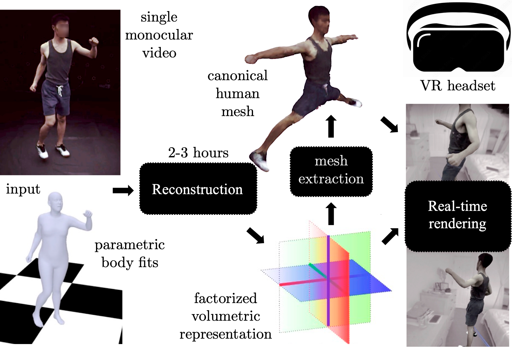
Figure 1: Given a monocular video with a SMPL parametric body fit, our method quickly reconstructs a 3D model of the person in canonical pose using a factorized radiance field representation [5]. Then, it extracts a tight rigged mesh and uses a new local ray-marching render which, without baking or otherwise converting the radiance field, can render the dynamic human on a consumer VR device at 40FPS. Videos and demos are available at https://real-time-humans.github.io/.

Emerging technologies such as virtual and mixed reality make photorealistic 3D reconstruction increasingly relevant and impactful. We can envisage a future in which, instead of taking pictures or movies with smartphone cameras, anyone will be able to capture and experience full $360^{\circ}$ holograms with equal quality, simplicity, and generality. However, despite recent progress in methods such as neural rendering, we remain quite far from this objective.

Many neural rendering approaches assume static scenes and the availability of dozens if not hundreds of input views for each reconstructed scene [24, 1, 2, 31, 32, 38]. Many dynamic extensions of neural rendering [26, 27, 30, 21, 25] handle small deformations. The most interesting content, however, is highly dynamic and often involves people. This has motivated the development of specialised models that can account for the highly-deformable structure of such objects, but most of these still assume that scenes are captured from multiple cameras [22, 29, 20, 44], which is incompatible with consumer applications. When data is captured by a smartphone or pair of AR glasses, only a single slowly-varying viewpoint is available for 3D reconstruction.

A few methods such as HumanNeRF-UW [41], A-NeRF [36] and NeuMan [17] can obtain photorealistic reconstructions of articulated humans from such monocular videos. These methods use articulated human models such as SMPL [23] to define a scaffold to model the object deformation, using a pre-trained predictor to obtain an initial estimate of the 3D body shape and pose. Then, they capture the shape of the subject over time as a deformation of a canonical radiance field, which is time-invariant. Unfortunately, jointly learning a radiance and deformation fields with a neural network requires several days of optimization to reconstruct a single monocular video. Furthermore, 3D video playback using the standard emission-absorption method is also slow due to the necessity of evaluating the neural network hundreds of times for each rendered pixel.

In this paper, we reconsider these architectures and we improve them significantly in terms of training and rendering speed, achieving fast training and real-time rendering. This is achieved by three design decisions, discussed next.

First, instead of representing the radiance field with a neural network, we use a tensor-based decomposition of the field, inspired by [5, 33, 4]. This representation leads to faster convergence than when using an MLP.

Second, we directly leverage linear blend skinning (LBS) in SMPL to model motion during training and rendering. This differ from previous approaches that trained a module to invert SMPL [41, 20] or learned a 3D scene flow field using a separate MLP [41, 22, 17], which is costly. Instead, we map each 3D point to canonical space solely by approximating the inverse LBS function using the inverse transformation of the closest SMPL face. This approximation is good where it matters, namely when the queried 3D point is already in the vicinity of the body surface.

Third, we propose to extract a personalized human mesh template from the reconstructed human in the factorized radiance field. During training, the exact shape of the person is not known, and the continuous volumetric representation allows to learn it though back-propagation. However, neural rendering requires sampling the full estimated object bounding box, which is too slow for real-time rendering. After the training is completed, we thus extract a mesh that is close to the surface of the reconstructed person. This mesh can then be used as a tight scaffold to implement neural rendering efficiently on device. Specifically, we describe a new local ray marching algorithm that carries out, using a custom shader, ray marching and emission absorption on a short distance from the mesh triangles as these are processed by the GPU rasteriser. Compared to other recent hardware-accelerated neural rendering techniques, our technique avoids baking, i.e., sampling the radiance field values and storing them in a different specialized data structure, which is usually expensive and lossy. Instead, it displays the unmodified radiance field directly.

To summarize, our contributions are the following: 1. We show that adopting a factorized radiance field representation and a simple LBS-based deformation model allows for fast reconstruction ($24$ times faster than HumanNeRF-UW) with comparable or better rendering quality on the ZJU-Mocap [29] scenes. 2. We show that it is possible to extract a canonical mesh from the learned radiance field, together with a rig derived from the LBS model in SMPL, which approximates well each individual. 3. We show that, given these design choices, it is possible to use GPU hardware to renderer the deformable radiance field model preserving quality while achieving real-time playback (at 40 FPS on the mobile GPU of a consumer VR device), which is three orders of magnitude faster than the HumanNeRF-UW approach (0.05 FPS).

2 Related work

Reconstructing humans from single images.

Performing 3D reconstruction of humans from single images is ill-posed and requires leveraging prior information on human geometry and poses. Several methods [3, 37, 19] use the SMPL model [23] as prior, but they result in only approximate reconstructions which are insufficient for VR/AR applications. PIFu [33, 34] directly predicts a volumetric representation of a human from a single RGB image using an MLP, but generalizes poorly beyond the training data distribution. ARCH [16, 14] combines parametric models and implicit function representations to obtain higher fidelity reconstructions, which are also rigged and animatable, but achieve limited overall quality due to the fact that they use a single image and cannot take advantage of video data.

Reconstructing humans from multiple videos.

In order to obtain higher quality reconstructions, several methods [22, 29, 20, 44] leverage multiple synchronized videos. Neural Actor [22] learns neural radiance fields [24] to model a human in canonical pose, and uses the inverse linear blend skinning (LBS) transform from SMPL to map between posed and canonical spaces. TAVA [20] uses a similar approach, but proposes to learn the inverse LBS weights and use Mip-NeRF [1] instead of vanilla NeRF. Neural Body [29] attaches neural codes to the SMPL vertices, poses them, and converts them to a full volumetric representation of the radiance field using a 3D sparse CNN [13, 9]. HumanNeRF-ShanghaiTech [44] combines NeRF and the inverse LBS mapping (as in Neural Actor), but conditions the NeRF model on features sampled from neighbouring input views similar to IBRNet [39] for rigid scenes. However, these methods require multiple views, and are thus inapplicable when only a monocular sensor is available.

Reconstructing humans from monocular videos.

Recent methods considered 3D human reconstruction from monocular videos. Vid2Actor [40] extracts from SMPL a motion basis, uses it for inverse LBS, and trains two 3D CNNs to regress the inverse LBS weights in posed space and the density and color of the canonical human. HumanNeRF-UW [41] extends Vid2Actor by replacing their voxel-grid representation with a coordinate MLP and further refine deformations using SMPL pose refinement and a non-rigid scene-flow MLP. A-NeRF [36] computes codes of the posed 3D points that are relative to the SMPL skeleton and use those to construct a pose-dependent NeRF model (somewhat analogously to the approach used in Neural Body). NeuMan [17] decomposes the scene into a static background component and the foreground dynamic human, and learns a different NeRF model for each component separately. They use inverse LBS for warping points from posed to canonical space and a standard NeRF MLP for modelling the canonical human.

While powerful, these models are typically very slow to train (sometimes in the order of days on a single GPU) and to render, making them unsuitable for playback in mobile devices such as in VR headsets.

Real-time neural and volumetric rendering.

Most of the works discussed above represent radiance fields using MLPs and use raymarching for rendering. Hence, the MLPs need to be evaluated hundreds of time for each pixel, which requires seconds for each rendered image. For real-time rendering, several methods have proposed to “bake” or cache the NeRF MLP [15, 42, 11]. However, such representations are memory intensive, do not support dynamic content, and require a high-end GPU for achieving real-time rendering.

Closer to ours, MobileNeRF [7] leverages the fast triangle rasterization hardware in modern GPUs for real-time rendering of NeRF, but with substantial differences. They also need to “bake” the radiance field into an especially-crafted mesh to avoid emission-absorption rendering. Because they change the rendering model, they require a conversion step that involves further learning and approximations, which also does not support dynamic content. In contrast, our technique renders in real time the original dynamic radiance field, accelerating emission absorption. Because we load the original model into the GPU, we do not require conversion, and we can preserve the shape and appearance details in the source radiance field with only minor approximations. As far as we are aware of, our method is the first one to be able to render dynamic radiance fields in real-time on mobile hardware without resorting to baking.

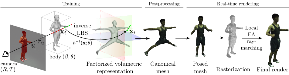
Figure 2: Overview of the proposed method. During training, we shoot rays from the training cameras onto the scene and sample points withing the bounding box of the parametric human body mesh. Points which are close to the mesh are warped to canonical space via inverse linear-blend-skinning (LBS), where the factorized volumetric representation is sampled for density and color, and whose values are used to perform raymarching. After training, a canonical mesh is extracted from the learnt factorized volumetric representation. For real-time rendering, the canonical mesh is posed, rasterized, and used to guide the inverse skinning and local raymarching.

3 Fast reconstruction of dynamic humans

Our method leverages recent progress in neural fields and monocular 3D reconstruction in order to allow for fast 3D reconstruction of humans from monocular videos and corresponding parametric SMPL fits. During reconstruction, our method employs the following modules: (i) a factorized volumetric representation that learns the shape and color of the human in canonical pose, (ii) a deformation module which performs inverse linear blend skinning to map 3D points from posed space to canonical space. In addition, we propose (iii) a rasterization-based method for rendering the trained model in real-time. Our full model is illustrated in Fig. 2. Each of these components is presented next in more detail.

3.1 Factorized volumetric radiance fields

In this work, we leverage recent progress on neural radiance fields [24, 5] as a continuous and differentiable representation for modeling shape and color. Next, we review these models and present the factorized formulation that we adopt in this work.

Radiance fields.

An image $I:\Omega\rightarrow\mathbb{R}^{3}$ is a map from pixels $u\in\Omega=[0,\dots,W]\times[0,\dots,H]$ to corresponding colors $I(u)\in\mathbb{R}^{3}$. The camera projection function $\pi:\mathbb{R}^{3}\rightarrow\mathbb{R}^{2}$ is a map from 3D points $\bm{x}\in\mathbb{R}^{3}$ in the world space to corresponding pixels (image points) $u\in\mathbb{R}^{2}$. A radiance field is a pair of functions mapping each 3D point $\bm{x}$ to a corresponding density $\sigma(\bm{x})\in\mathbb{R}_{+}$ and corresponding color $c(\bm{x})\in\mathbb{R}^{3}$.

The color of a pixel $u$ is obtained by marching along the ray $r_{u}$ originating from the camera center and propagating in the direction of pixel $u$ (interpreted as a 3D point). Let $(\bm{x}_{i})_{0}^{N-1}$ be a sequence of $N$ samples along ray $r_{u}$ separated by steps $\Delta$. The color of pixel $u$ is extracted from the radiance field via the following emission-absorption rendering equation:

$$I(u)=\sum_{i=0}^{N-1}(T_{i}-T_{i+1})c(\bm{x}_{i}),~{}~{}~{}T_{i}=e^{-\Delta\sum_{j=0}^{i-1}\sigma(\bm{x}_{i})}.$$ (1)

where $T_{i}$ is the accumulated transmittance up to $\bm{x}_{i}$, namely the probability that a photon is transmitted from point $\bm{x}_{i}$ back to the camera center without being absorbed.

Deformable radiance fields.

The radiance field of eq. 1 could be extended to represent the different poses of an articulated object by adding the object’s pose parameters $\theta$ as an additional parameter of the density $\sigma(\bm{x};\theta)$ and color $c(\bm{x};\theta)$ functions. Modelling such functions directly, however, would be statistically inefficient because it would not account for the fact that the different poses are not arbitrary, but related by geometric deformations.

Therefore, in this work we adopt more efficient approach with considers canonical density $\bar{\sigma}(\bar{\bm{x}})$ and color $\bar{c}(\bar{\bm{x}})$ fields that are pose-invariant and, separately, a posing function $\bm{x}=h(\bar{\bm{x}};\theta)$ mapping points $\bar{\bm{x}}$ from the canonical space to their posed locations $\bm{x}$. The pose-dependent fields are the composition of the pose-invariant fields and of the inverse of the posing function:

$$\sigma(\bm{x};\theta)=\bar{\sigma}(h^{-1}(\bm{x};\theta)),~{}~{}~{}c(\bm{x};\theta)=\bar{c}(h^{-1}(\bm{x};\theta)).$$ (2)

Tensorial fields.

We leverage the recent factorized volumetric neural field formulation from TensoRF [5] to represent the shape and color of the canonical human.

In order to model the field $(\sigma,c)$, we do not use the standard approach of adopting an MLP and positional encoding [24], but use instead the TensoRF parameterization. Specifically, we consider a voxel grid of resolution $D\times H\times W$ and further decompose it as the sum of three matrix-vector products:

$$\bar{\sigma}(\bar{\bm{x}})\!=\!\rho\left(\sum_{r=1}^{R_{\sigma}}\!M^{YX}_{r,\bar{y},\bar{x}}v^{Z}_{r,\bar{z}}\!+\!M^{YZ}_{r,\bar{y},\bar{z}}v^{X}_{r,\bar{x}}\!+\!M^{XZ}_{r,\bar{x},\bar{z}}v^{Y}_{r,\bar{y}}\!\right)\!.$$ (3)

Here $\bar{\bm{x}}=(\bar{x},\bar{y},\bar{z})$, $r$ is the channel index, and the sub-indices indicate the tensor sampling position. In addition, $M^{YX}$ is a $R_{\sigma}\times H\times W$ tensor, $v^{Z}$ a ${R_{\sigma}}\times D$ matrix, and the other terms follow a similar pattern, so in total there are $R_{\sigma}(HW+HD+WD+H+W+D)$ parameters only, far less than $HWD$ as long as the number of components $R_{\sigma}\ll(HWD)^{\frac{1}{3}}$. The activation function $\rho(a)=\log(1+\exp(Ga))$ is the softplus operator with a fixed gain $G\approx 1/\Delta$, where $\Delta$ is the step between ray samples.

The color field $\bar{c}$ is defined in a similar manner, for each of the three RGB components, and uses the sigmoid as activation function.

The adoption of these factorized representation not only allows for faster training compared to the MLP-based models, but is particularly suitable for fast real-time rendering by storing the different tensor factors as textures that are naturally interpolated by the graphic shaders of GPUs (cf. Sec. 4).

3.2 Skinning-based deformation module

Several previous works use MLP-based deformation models [26, 27, 41, 22, 17], alone, or in conjunction with articulated deformations [22, 41, 17]. Because these models are slow to evaluate, we propose to use only a linear blend skinning (LBS) articulated deformation model, and show that this simple deformation model can still achieve competitive results while being much simpler and allowing for real-time rendering. We next review LBS and present our proposed approach.

Posing via blend skinning.

Given that humans are articulated objects, we leverage the parametric SMPL model [23] and the linear blend skinning formulation which allows to easily build the posing function $h$, given the SMPL template mesh model and the pose parameters. In particular, the SMPL model provides a template mesh $\mathcal{M}=(\mathcal{V},\mathcal{F})$ with points ${\bar{\bm{v}}}\in\mathcal{V}\subset\mathbb{R}^{3}$ and triangular faces $f\in\mathcal{F}$. In addition, the template mesh is associated with a skeleton, which is a collection of bones $b\in\{1,\dots,B\}$ whose angles define the pose parameters. Each template vertex $\bar{\bm{v}}$ is softly attached to the different bones by its skinning weights $w(\bar{\bm{v}})\in\mathbb{R}_{+}^{B}$. Then, the posed vertices can be obtained by an affine map $\bm{v}=h(\bar{\bm{v}};\theta)=A(\bar{\bm{v}};\theta)\bar{\bm{v}}\$, where:

$$A(\bar{\bm{v}};\theta)=\sum_{b=1}^{B}w_{b}(\bar{\bm{v}})A_{b}(\theta),$$ (4)

and $A_{b}(\theta)$ is the affine transform associated to bone $b$ for the pose $\theta$. More details are provided in Appendix A.1.

Volumetric and inverse blend skinning.

Skinned models like SMPL only define the skinning weights $w(\bar{\bm{v}})$ for the vertices of the template mesh, which approximates the real object surface. However, because the radiance field is a volumetric representation, we need transformations to be defined around the object surface, and not just on the surface, and thus the skinning weights need to be extended to nearby 3D points. Furthermore, in order to perform ray marching and compute the pose-invariant fields from eq. 2, we need to map points $\bm{x}$ from the posed space back to canonical space, and therefore knowledge of the posing function $h(\bar{\bm{x}};\theta)$ is not enough; instead, we require its inverse:

$$\bar{\bm{x}}\!=\!h^{-1}(\bm{x};\theta)\!=\!A(\bar{\bm{x}};\theta)^{-1}\!\bm{x}\!=\!\!\left[\sum_{b=1}^{B}w_{b}(\bar{\bm{x}})~{}\!A_{b}(\theta)\right]^{-1}\!\!\!\!\!\!\!\cdot\bm{x}.$$ (5)

Because $\bar{\bm{x}}$ appears on the l.h.s. and r.h.s. of this expression, this defines $\bar{\bm{x}}$ as the solution to an equation which cannot be solved in closed form. Prior works [10, 6] addressed these issues by learning the extended skinning weights and/or the inverse posing function, but these approaches increase the complexity of the model and therefore the training and rendering time.

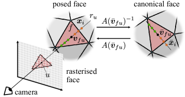
Figure 3: Real-time radiance fields via rasterization. The posed face $f$ is used to determine the portion of the radiance field that is likely to affect given pixel $u$ and to map computations to the rasterization unit of the GPU.

In contrast, we employ the approach introduced in [22], where the inverse transformation of a point $\bm{x}$ is approximated to that of the closest mesh vertex $\bar{\bm{v}}_{i^{*}}$:

$$\bar{\bm{x}}=h^{-1}(\bm{x};\theta)\approx A(\bar{\bm{v}}_{i^{*}};\theta)^{-1}\bm{x},$$

$$\text{s.t.}~{}i^{*}=\operatornamewithlimits{argmin}_{i}\|\bm{x}-\bm{v}_{i}\|_{2}.$$ (6)

This approximation is only valid locally, and therefore only applied to ray points $\bm{x}$ where the distance to the closest vertex is below a threshold $\tau$. Otherwise, points are discarded and not used for raymarching, which is equivalent to setting $\sigma(\bm{x};\theta)=\mathbf{1}_{[d(\bm{x},{\bm{v}}_{i^{*}})\leq\tau]}~{}\bar{\sigma}(h^{-1}(\bm{x};\theta)).$

Contrary to prior work, we do not combine this deformation with any additional trainable model, in order to allow for real-time evaluation of the deformation model in mobile hardware. Our experimental results show that our method performs similarly to prior state-of-the-art despite of this simplified deformation model.

4 Real-time dynamic radiance fields

The factorized radiance field and deformation model presented in Sec. 3.1 and Sec. 3.2 were chosen specifically to allow for real-time rendering, through a customized GPU shader program that implements an efficient local emission-absortion raymarching. Our approach avoids baking or conversion steps and allows to replay the original radiance field with only minor approximations.

Customized human mesh.

Our proposed local raymarching is guided by an initial rasterization step of the posed mesh. In order to handle occlusions and object boundaries properly, we replace the SMPL mesh with one that more accurately approximates the body shape at rest, and transfer to the SMPL joints and blendshapes so that it is fully-rigged and amenable for posing.

We extract this mesh from the radiance field by: (i) rendering frames with masks and depth-maps from the canonical model, (ii) unprojecting these depth maps to form a dense point cloud and, (iii) converting this point cloud onto a mesh. An example of the extracted mesh is shown on Fig. 2. Please refer to the Appendix A.2 for further details.

Rasterization of the posed mesh.

Without any guidance, volumetric rendering using eq. 1 requries to sample hundreds of ray points for each generated pixel. For an opaque object, this is extermely inefficient, as only a tiny fraction of those samples land close enough to the surface to make a significant contribution to the final color. Instead, we resort to rasterization of the customized posed mesh as an initial step of our rendering pipeline, which provides guidance for performing a local volumetric rendering.

In this case, the rasterizer iterates over the triangles $f\in\mathcal{F}$ of the mesh, quickly finding the pixels $u$ that are contained in them (Fig. 3). The rasterizer also quickly computes the barycentric coordinates $\alpha_{i}$ of the 3D face point $\bm{v}_{fu}\in f$ that projects onto pixel $u$, defined as:

$$\bm{v}_{fu}=\sum_{i=1}^{3}\alpha_{i}\bm{v}_{fi},~{}~{}~{}\alpha_{i}\geq 0,~{}~{}~{}\sum_{i=1}^{3}\alpha_{i}=1,$$ (7)

where $\bm{v}_{fi}$ are the three mesh vertices. Then, the color $I(u)$ of the pixel is obtained by computing the color $c(\bm{v}_{fu})$ of point $\bm{v}_{fu}$. This calculation is done in parallel for all pixels using a shader program running in the GPU.

Local emission-absorption raymarching.

Instead of computing the color $c(\bm{v}_{fu})$ by using an UV-texture mapping, as it is usually done for coloring meshes, we compute $c(\bm{v}_{fu})$ by performing a local emission-absorption raymarching in the vicinity of point $\bm{v}_{fu}$, as illustrated in Fig. 3.

In practice, we first map the point $\bm{v}_{fu}$ from the posed mesh to its counterpart in canonical space $\bar{\bm{v}}_{fu}$ by applying the transformation $A(\bar{\bm{v}}_{fu})^{-1}$. For this, $A(\bar{\bm{v}}_{fu})^{-1}$ is efficiently and automatically approximated by the vertex shader through barycentric interpolation, by storing the inverse transformation $A(\bar{\bm{v}})^{-1}$ of each vertex $\bar{\bm{v}}\in\mathcal{V}$ as a vertex property.

Once $\bar{\bm{v}}_{fu}$ is computed, we can consider a small number of samples $\bar{\bm{x}}_{i}$ (as illustrated in the right side of Fig. 3) to perform local emission-absorption raymarching. For this, the evaluation of the factors $M$ and $v$ of the density and color for fields can be done very efficiently on the GPU by mapping these 2D and 1D tensors to 2D and 1D textures maps and using the native GPU texture sampling functions.

Once the densities and colors are computed for all samples $\bar{\bm{x}}_{i}$ in the local ray segment, eq. 1 is used to obtain the final pixel color $I(u)$.

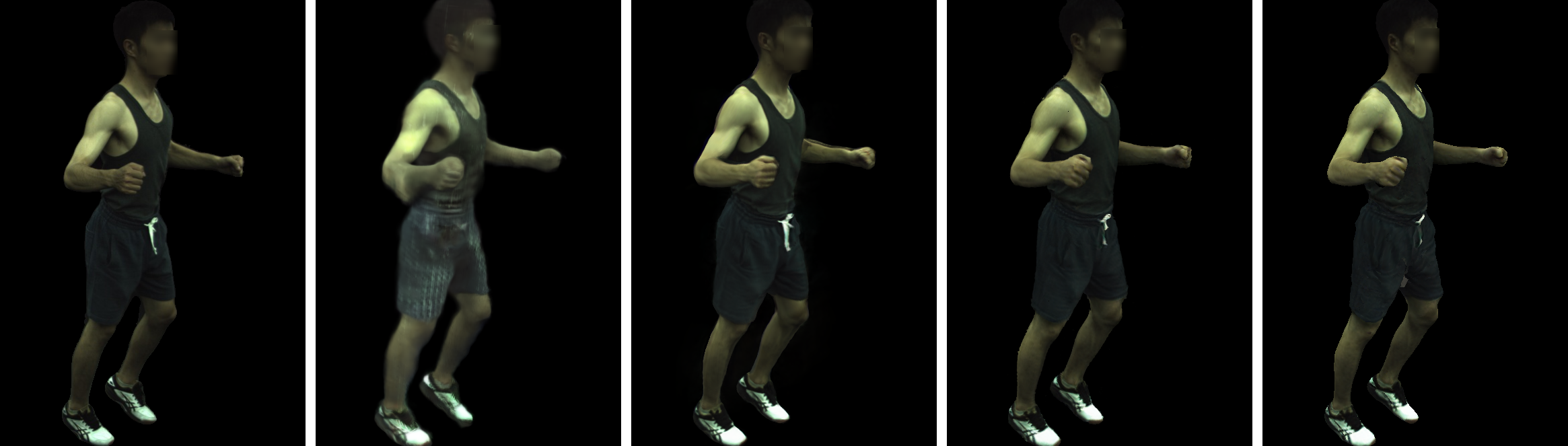
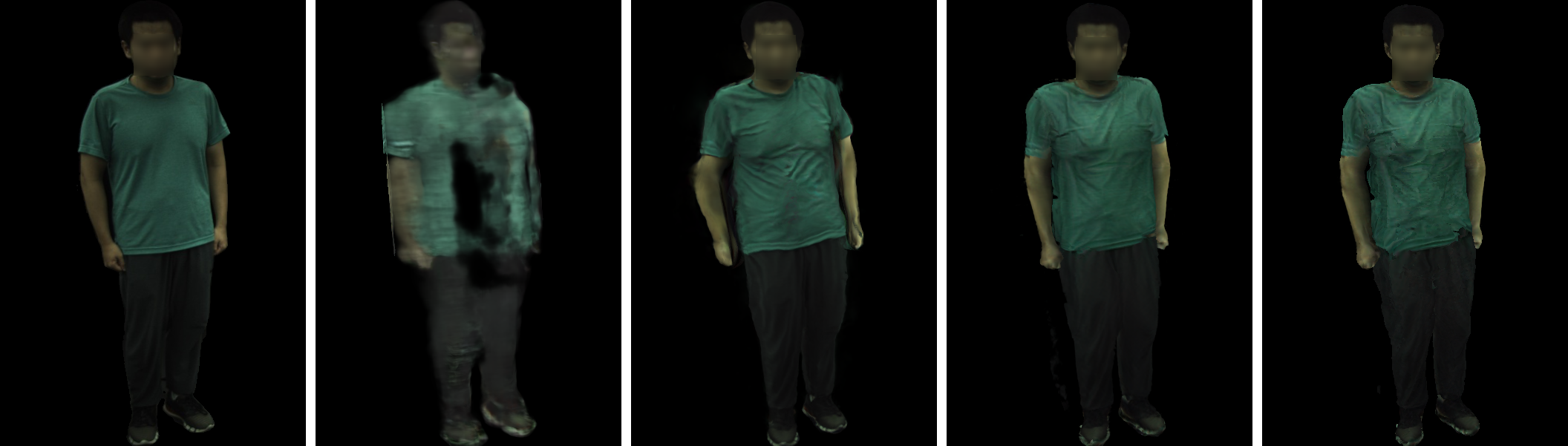
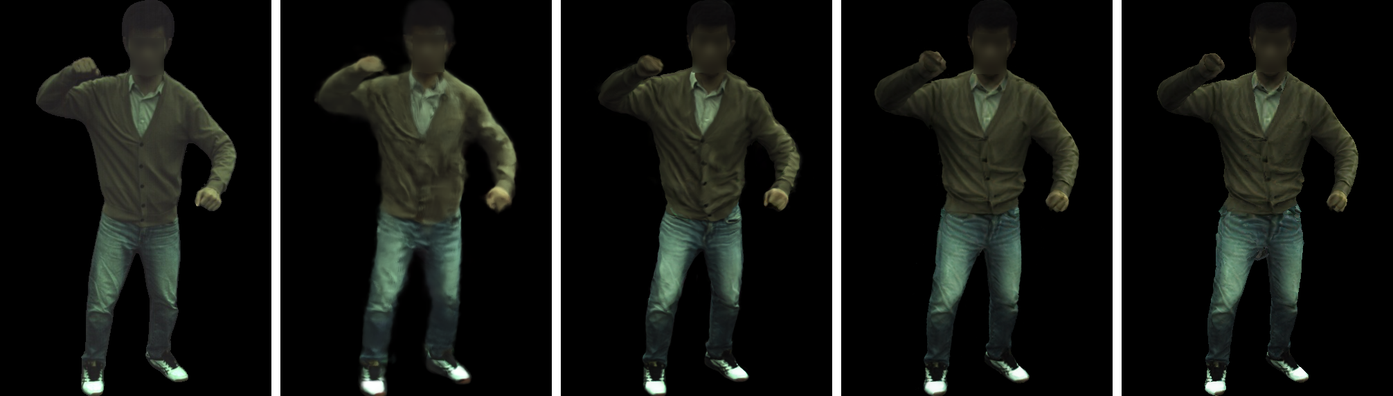
(a) Ground-truth

(b) NeuralBody [29]

(c) HumanNeRF-UW [41]

(d) Ours - reconstruction

(e) Ours - real-time

Figure 4: Qualitative results on ZJU-Mocap. We show a qualitative comparison between our proposed method and other state-of-the-art methods on test images. Our method produces sharp images, perceptually similar to those of HumanNeRF-UW, despite presenting a simpler deformation model. Faces have been blurred for privacy reasons.

	LPIPS*1000 $\downarrow$						PSNR $\uparrow$						SSIM $\uparrow$
	Sequence ID						Sequence ID						Sequence ID
Method	377	386	387	392	393	394	377	386	387	392	393	394	377	386	387	392	393	394
Neural Body (14h)	43.08	48.08	57.34	50.39	57.09	54.36	28.87	30.12	26.76	29.84	27.80	28.90	0.9609	0.9588	0.9462	0.9575	0.9472	0.9497
HumanNeRF-UW (72h)	30.28	34.16	41.10	36.24	40.30	38.12	30.19	32.83	28.06	30.91	28.44	30.47	0.9642	0.9669	0.9551	0.9641	0.9544	0.9567
Ours - reconstruction (2-3h)	27.72	34.42	43.44	35.68	41.28	38.00	30.00	32.90	28.08	31.08	28.51	30.28	0.9710	0.9687	0.9545	0.9645	0.9535	0.9564
Ours - real-time (40FPS)	32.76	35.01	42.87	37.79	41.86	40.53	28.42	32.19	27.76	30.35	27.91	29.46	0.9671	0.9677	0.9540	0.9635	0.9531	0.9555

Table 1: Results on the ZJU-mocap benchmark. Our method obtains the best reconstruction results on most of the scenes on the PSNR metric, and on half of the scenes, with respect to the LPIPS and SSIM metrics, while being significantly faster to train (2–3h vs 14h or 72h). Our real-time variant introduces a small performance drop but mantains similar visual quality (cf. Fig. 4).

Limitations.

The proposed local emission-absorption raymarching relies on the rasterization of the posed customized human mesh to define the local ray segments where ray marching is performed. This can cause small issues around occlusion boundaries, if the estimated mesh is either too small or too large. If the occluding part of the object is too small, the render will show a slight “loss of mass” when rendered. If it is too large, this additional occluding part of the object will produce ”black pixels”, which should in reality show the background part of the object. This issue is minimized by making the scaffold as tight as possible.

5 Experimental evaluation

In order to demonstrate the performance of our proposed method, we evaluate results on two different benchmarks, the ZJU-Mocap scenes and the NeuMan scenes. In addition, we show the results of the proposed on-device real-time renderer and ablations on the color model employed by the factorized volumetric representation.

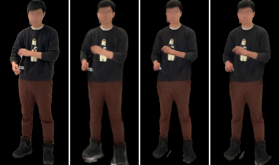
Ground-truth

NeuMan

Ours - recon.

Ours - real-time

Figure 5: Qualitative results on NeuMan scenes. Our method obtains state-of-the-art visual quality, comparable to that of NeuMan, while being fast to train and render. Faces have been blurred for privacy reasons.

	LPIPS*1000 $\downarrow$						PSNR $\uparrow$						SSIM $\uparrow$
	Sequence name						Sequence name						Sequence name
Method	bike	citron	jogging	lab	parkinglot	seattle	bike	citron	jogging	lab	parkinglot	seattle	bike	citron	jogging	lab	parkinglot	seattle
NeuMan	44.65	28.00	41.53	43.38	44.23	24.23	26.73	27.88	26.31	28.37	27.43	27.80	0.9521	0.9633	0.9496	0.9593	0.9581	0.9687
Ours - reconstruction	49.63	29.60	42.00	42.18	49.24	19.76	26.37	26.60	25.88	28.29	24.12	28.43	0.9465	0.9588	0.9461	0.9574	0.9524	0.9722
Ours - real-time	48.04	31.43	41.86	42.71	56.54	21.14	25.86	26.12	25.13	27.39	23.12	27.86	0.9457	0.9580	0.9451	0.9552	0.9438	0.9706

Table 2: Quantitative results on the NeuMan benchmark. Our method obtains comparable reconstruction performance to NeuMan [17] for most sequences, with superior performance for seattle, while having real-time rendering capabilities without significant loss in visual quality (cf. Fig. 5).

Implementation details.

We implement our model using PyTorch [28]. In particular, we use 8 channels for modeling density and color ($R_{\sigma}{=}R_{c}{=}8$) in the tensorial model. In addition, we use a coarse-to-fine training approach, increasing the voxel grid resolution $D\times H\times W$ several times during training, following [5]. We begin training with a resolution $HWD=10^{6}$ and end with $HWD=4.096\times 10^{6}$, scaled accordingly to the person’s bounding box. At each training iteration, a batch of training rays $r_{u}$ is constructed by sampling six $32\times 32$ image patches, each centered around a foreground point. The models are trained for 30 epochs of 1000 iterations each, regardless of the number of training images. Before posing the SMPL template with the provided $\theta_{\text{data}}$ parameters from each dataset, we compute a small refinement $\theta_{\text{ref}}$ using a 4-layer MLP with 256 hidden units, following [41]. The final body parameters are thus $\theta=\theta_{\text{ref}}\circ\theta_{\text{data}}$. The factorized neural field and the pose correction MLP are trained jointly. For training, we employ a photometric loss, a sparsity regularization loss, as well as a perceptual loss (LPIPS). The whole training procedure takes between 2 and 3 hours on a single modern GPU.

ZJU-Mocap benchmark.

We first evaluate our method on the ZJU-Mocap dataset introduced in [29]. We follow the evaluation protocol from [29] and, for each sequence, use images from 19 unseen cameras for testing, sampled at a 30 frames interval for the first 300 frames, giving 190 test images per sequence. Following [41], we evaluate on 6 sequences, identified by their sequence IDs (377, 386, 387, 392, 393, and 394). In Tab. 1 and Fig. 4 we present the quantitative and qualitative results of our method compared to NeuralBody [29] and HumanNeRF-UW [41]. We present results both for the reconstruction phase (Sec. 3) using standard emission-absorption raymarching and for the proposed real-time rendering (Sec. 4) that can run at 40FPS on mobile hardware. Our reconstructions obtain the best PSNR results for most of the scenes, and best LPIPS and SSIM results for half of the scenes, while being significantly faster to train than the baselines (2–3h for our method vs. 72h for HumanNeRF-UW and 15h for Neural Body). In addition, we observe that the rasterization-guided raymarching introduces a small performance loss, while allowing for real-time rendering. As shown in Fig. 4, the visual quality of our reconstuction and real-time variants is on-par or superior to previous methods.

NeuMan benchmark.

In addition, we evaluate our method on the scenes from NeuMan [17]. The NeuMan method uses a NeRF [24] module to model the background scene, which is used for segmenting the person. As our model does not explicitly model the background, we use XMeM [8] to segment the foreground person by scribbling the first frame of each sequence and propagating results automatically. The results in Tab. 2 show that our reconstructions outperform NeuMan on two scenes according to LPIPS, and are slightly inferior for the other four scenes. Nevertheless, qualitative results from Fig. 5 show that the perceptual quality of our method is similar to that of NeuMan, even for our real-time renders.

	Color model	Pose correction	LPIPS 1000 $\downarrow$	PSNR$\uparrow$	SSIM$\uparrow$
Ours - recon.	Direct	Yes	36.76	30.14	0.9614
FA-Spherical Harm.	SH	Yes	36.97	30.17	0.9612
FA-MLP color	MLP	Yes	37.57	30.20	0.9616
FA-No pose corr.	Direct	No	38.63	29.95	0.9607

Table 3: Ablation study. We analyze the performance drop incurred by modifying several components of the proposed method. We show the mean LPIPS, PSNR and SSIM metrics over all ZJU-Mocap sequences.

Model ablations.

We also evaluate the effect of modifying the color model of the factorized volumetric representation. In Sec. 3.1 we proposed to model color directly, i.e. outputting RGB values directly from the factorized volumetric representation. Alternatively, we can have the factorized representation output spherical harmonic coefficients or color descriptors which are then used to and compute the final RGB values via spherical harmonic functions or a small color MLP, respectively. The results of using these different color models are presented in Tab. 3. We observe that the choice of the color model does not affect performance significantly. We therefore propose to use direct color prediction (RGB values), for its simplicity compared to using spherical harmonics or MLP for color prediction, allowing for faster real-time rendering. Finally, we observe that disabling the body pose correction also diminishes performance to a small extent.

6 Conclusion

We have introduced a method capable of learning neural radiance fields of articulated humans from monocular videos. By adopting a factorized radiance field model and a simple deformation model, we were able to cut down the training time by an order of magnitude or more compared to prior work, while matching these methods in visual quality. Furthermore, we have introduced a novel approach to render these dynamic reconstructions in real-time on a mobile GPU. This is done through a rasterization-guided local raymarching which leverages a refined customized human mesh for rendering the neural radiance field without resorting to baking, and with minimal loss of quality. As far as we know, this is the first work to perform realtime rendering of dynamic humans in mobile hardware using radiance fields, and without resorting to baking. We hope this work will inspire other future work in this area.

Appendix A Additional technical details

A.1 Linear blend skinning

Given a canonical mesh and its associated skeleton, which is a collection of bones $b\in\{1,\dots,B\}$, and the pose parameters $\theta$, which are the rotations of the bone joints, linear blend skinning (LBS) allows to pose the canonical mesh using the pose parameters alone. In order to account for transitions between bones, each canonical vertex $\bar{\bm{x}}$ is not assigned to a single bone, but rather softly attached to different bones by its skinning weights $w(\bar{\bm{x}})$.

Bones form a tree, where $b^{\prime}=\operatorname{par}(b)$ denotes the parent of bone $b$, except for the root bone $b=1$ which has no parent.

Then, given a 3D point $\tilde{\bm{x}}$ defined in the reference frame of bone $b$, we can express it in the reference frame of the parent bone as $\bm{x}^{\prime}=g_{b}(\theta)\tilde{\bm{x}}$, where $g_{b}(\theta)\in SE(3)$ is the rigid transformation between the two bones. Hence, the pose vector $\theta$ specifies three rotation angles for each transformation $g_{b}$ (the translation component is given by the parent bone’s length); only for the root transformation $g_{1}$, which positions the skeleton in world space, $\theta$ specifies the translation component as well. In order to express the 3D point in world coordinates $\bm{x}=G_{b}(\theta)\tilde{\bm{x}}$, we compose recursively the transformation towards the root:

$$G_{b}(\theta)=G_{\operatorname{par}(b)}(\theta)\circ g_{b}(\theta),~{}~{}~{}G_{1}(\theta)=g_{1}(\theta).$$

Consider now a 3D point $\bar{\bm{x}}$ in canonical space, rigidly attached to bone $b$. In order to pose it, we first express it relative to its bone as $\tilde{\bm{x}}=G_{b}^{-1}(\theta_{0})\bar{\bm{x}}$, where $\theta_{0}$ is the canonical pose. Then, we map it to world space by as $\bm{x}=G_{b}(\theta)\tilde{\bm{x}}$. In practice, each point $\bar{\bm{x}}$ is attached to all bones to a degree expressed by the skinning weights $w(\bar{\bm{x}})\in\mathbb{R}^{B}$, which are non-negative and sum to one. The individual maps are linearly combined (called blend skinning), resulting in the affine map

$$A(\bar{\bm{x}};\theta)=\sum_{b=1}^{B}w_{b}(\bar{\bm{x}})~{}G_{b}(\theta)\circ G_{b}^{-1}(\theta_{0}).$$ (8)

For simplicity, in the main paper we consider the composed affine map for each bone $A_{b}(\theta)=G_{b}(\theta)\circ G_{b}^{-1}(\theta_{0})$, assuming $\theta_{0}$ as fixed.

Finally, the corresponding posing function resulting from linear blend skinning is

$$x=h(\bar{\bm{x}};\theta)=A(\bar{\bm{x}};\theta)\bar{\bm{x}}.$$ (9)

A.2 Customized human mesh extraction

While previous methods have used algorithms such as marching cubes to extract meshes from implicit volumetric representations, we propose to use a render-based approach instead, as our canonical model contains noise in the regions where no supervision was provided due to the threshold $\tau$. To this end, we render frames from the trained canonical factorized model, along with their depth maps and estimated foreground masks, with a circular camera trajectory around the object (in a turntable fashion).

The depth maps are computed by measuring the depth w.r.t. to the current camera of the expected termination $\hat{\textbf{x}}_{t}$ of each camera ray, defined as

$$\hat{\textbf{x}}_{t}=\sum_{i=0,\dots,N-1}(T_{i}-T_{i+1})\textbf{x}_{i},$$ (10)

as done in NeRF [21]. Similarly, the foreground masks are obtained by computing the expected ray opacity as

$$\hat{o}=\sum_{i=0,\dots,N-1}(T_{i}-T_{i+1})=1-T_{N},$$ (11)

The estimated object foreground masks are obtained by retaining the pixels where $\hat{o}>0.5$.

Then, each depth-map is unprojected using the camera parameters and combined with the color render to obtain a set of 3D points, which are then fused with those from other images to obtain a dense point cloud. This point cloud is finally filtered using the foreground masks, such that only points that are classified as foreground for all images are kept.

Next, this dense point cloud is converted into a mesh by applying the screened Poisson surface reconstruction algorithm [18], and simplified using an edge-collapse technique [12] such that the number of final faces is around  15K, which is on the order of magnitude to the template mesh in SMPL. The surface normals for the extracted canonical mesh are mapped to the surface normals of the closest vertices of the underlying SMPL template mesh. Note that these normals are not used for shading, but only for running the screened Poisson surface reconstruction.

Finally, in order to be able to perform skinning of the extracted canonical mesh, we transfer the skinning weights from the SMPL template using the nearest vertices. The process of canonical mesh extraction is illustrated in Fig. 6. Note that the colors of the extracted canonical mesh are solely used for visualization purposes, and not used in the proposed rasterization-based raymarching, which only requires the vertices and triangles of the canonical mesh to guide the raymarching on the factorized volumetric representation.

A.3 Training losses

We present some additional details about the losses used for training. At each training iteration, a batch $\mathcal{B}=\{\mathcal{P}_{i}\}_{i=1,\dots,6}$ of six image patches $\mathcal{P}$ of size $32\times 32$ is constructed, and the our proposed model is used to estimate the image color $I(u)$ for each pixel $u\in P$. Then we use three different loss terms for optimizing the proposed model: (i) a photometric loss $\mathcal{L}_{\text{rgb}}$, (ii) a perceptual loss (LPIPS) $\mathcal{L}_{\text{lpips}}$, and, (iii) a sparsity regularization loss $\mathcal{L}_{\text{sparse}}$. Our overall loss is thus:

$$\mathcal{L}(\mathcal{B})=\alpha\mathcal{L}_{\text{rgb}}(\mathcal{B})+\beta\mathcal{L}_{\text{lpips}}(\mathcal{B})+\gamma\mathcal{L}_{\text{sparse}},$$

with:

$$\mathcal{L}_{\text{rgb}}(\mathcal{B}) =\frac{1}{N}\sum_{u\in\mathcal{B}}\lVert I(u)-I_{\text{gt}}(u)\rVert_{2}^{2}$$ (12)

$$\mathcal{L}_{\text{lpips}}(\mathcal{B}) =\frac{1}{6}\sum_{\mathcal{P}\in\mathcal{B}}\text{LPIPS}_{\text{vgg}}(I(\mathcal{P}),I_{\text{gt}}(\mathcal{P}))$$ (13)

$$\mathcal{L}_{\text{sparse}} =\frac{1}{R_{\sigma}\cdot HWD}\sum_{(M,v)\in\mathcal{W}}\sum_{rxyz}(Mv)^{+},$$ (14)

where $N=6\times 32\times 32$ is the total number of pixels in the training batch, $\text{LPIPS}_{\text{vgg}}$ is the perceptual loss proposed in [43] using the VGG-Net feature extractor [35], and the sparsity loss is applied over all three factors $\mathcal{W}=\{(M^{YX},v^{Z}),(M^{YZ},v^{X}),(M^{XZ},v^{Y})\}$ of the implicit volumetric representation of the density $\sigma$, and across all channels $R_{\sigma}$. In addition, the coefficients $\alpha,\beta,\gamma$ which modulate each loss term vary as the training progresses, and we can therefore define them as functions of the training iteration $i=1,\dots,30\,000$:

$$\alpha(i) =\begin{cases}1-0.8\cdot i/10\,000&\text{if }i<10\,000\\ 0.2&\text{otherwise}\end{cases}$$ (15)

$$\beta(i) =\begin{cases}0.8\cdot i/10\,000&\text{if }i<10\,000\\ 0.8&\text{otherwise}\end{cases}$$ (16)

$$\gamma(i) =\begin{cases}0&\text{if }i<2\,000\\ 8\cdot 10^{-5}&\text{if }2\,000\leq i<4\,000\\ 5\cdot 10^{-5}&\text{otherwise}\end{cases}$$ (17)

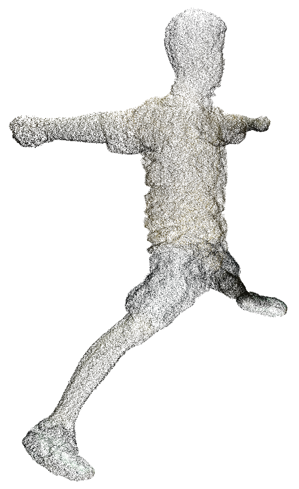
(a) Dense PCL	(b) Mesh (100K faces)	(c) Mesh (15K faces)

Figure 6: Canonical mesh extraction. We first generate a dense point cloud (a), from which we perform screened Poisson reconstruction (b), and, finally mesh simplification to 15K faces (c).

A.4 Proposed rasterization-guided local raymarching vs. phong shading

As an ablation study, we show in Fig. 7 the comparison of rendering the posed template mesh with our proposed method against using standard phong shading based on vertex colors. Note that as a texture of the human is not available, many details are lost when applying phong shading directly. In addition, this rendering technique requires an artificial light source and generates unrealistic reflection effects. On the contrary, our proposed method recovers the textures details from the learnt volumetric representation, and new views can be rendered directly without any additional artificial light source.

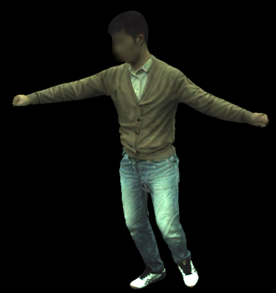
(a) Local volumetric rendering

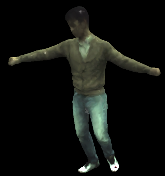
(b) Phong shading

Figure 7: Comparison between rendering techniques. We illustrate the results of the proposed local rasterization-based emission-absorption raymarching against rendering the template mesh directly with a standard phong shading.

Appendix B Demos and source code

B.1 VR Mixed reality demo

We have built a VR Mixed reality demo that demonstrates our proposed method, and rendering at 40FPS in consumer-level standalone VR headset, using the reconstructions obtained from the ZJU-mocap scenes.

Figure 8: VR Mixed reality demo. The dynamic human is rendered using VR-passthrough at 40FPS on a standalone VR device.

Several recordings of these scenes playing on the VR headset, as illustrated in Figure 8, are available in our website https://real-time-humans.github.io/. Note that the background scene is rendered in mixed reality thorough RGB passthrough using the VR headset’s frontal RGB camera, giving the effect of an AR device.

B.2 Desktop WebGL demo

Additionally we developed a Desktop WebGL demo that implements the proposed real-time volumetric rendering and runs inside the web browser, as illustrated in Figure 9. The demo is available in our website https://real-time-humans.github.io/.

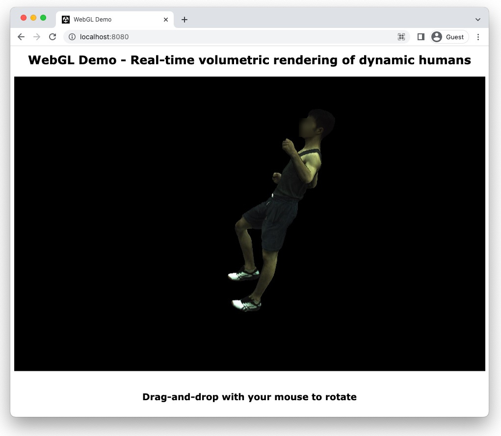
Figure 9: WebGL desktop demo. The demo is available in our website.

B.3 Source code.

We will release our source code to allow for reproducibility. It will be released under an open-source licence. The VR and WebGL demo apps will be released in binary format.

References

- [1] Jonathan T Barron, Ben Mildenhall, Matthew Tancik, Peter Hedman, Ricardo Martin-Brualla, and Pratul P Srinivasan. Mip-nerf: A multiscale representation for anti-aliasing neural radiance fields. In Proc. ICCV, 2021.
- [2] Jonathan T. Barron, Ben Mildenhall, Dor Verbin, Pratul P. Srinivasan, and Peter Hedman. Mip-nerf 360: Unbounded anti-aliased neural radiance fields. In Proc. CVPR, 2022.
- [3] Federica Bogo, Angjoo Kanazawa, Christoph Lassner, Peter Gehler, Javier Romero, and Michael J Black. Keep it SMPL: Automatic estimation of 3d human pose and shape from a single image. In Proc. ECCV, 2016.
- [4] Eric R Chan, Connor Z Lin, Matthew A Chan, Koki Nagano, Boxiao Pan, Shalini De Mello, Orazio Gallo, Leonidas J Guibas, Jonathan Tremblay, Sameh Khamis, et al. Efficient geometry-aware 3d generative adversarial networks. In Proc. CVPR, 2022.
- [5] Anpei Chen, Zexiang Xu, Andreas Geiger, Jingyi Yu, and Hao Su. TensoRF: Tensorial radiance fields. In Proc. ECCV, 2022.
- [6] Xu Chen, Yufeng Zheng, Michael J. Black, Otmar Hilliges, and Andreas Geiger. SNARF: differentiable forward skinning for animating non-rigid neural implicit shapes. arXiv.cs, abs/2104.03953, 2021.
- [7] Zhiqin Chen, Thomas Funkhouser, Peter Hedman, and Andrea Tagliasacchi. Mobilenerf: Exploiting the polygon rasterization pipeline for efficient neural field rendering on mobile architectures. arXiv preprint arXiv:2208.00277, 2022.
- [8] Ho Kei Cheng and Alexander G. Schwing. XMem: Long-term video object segmentation with an atkinson-shiffrin memory model. In Proc. ECCV, 2022.
- [9] Christopher Choy, JunYoung Gwak, and Silvio Savarese. 4d spatio-temporal convnets: Minkowski convolutional neural networks. In Proc. CVPR, 2019.
- [10] Boyang Deng, John P. Lewis, Timothy Jeruzalski, Gerard Pons-Moll, Geoffrey E. Hinton, Mohammad Norouzi, and Andrea Tagliasacchi. NASA: Neural articulated shape approximation. In Proc. ECCV, 2020.
- [11] Stephan J Garbin, Marek Kowalski, Matthew Johnson, Jamie Shotton, and Julien Valentin. FastNeRF: High-fidelity neural rendering at 200fps. In Proc. ICCV, 2021.
- [12] Michael Garland and Paul S Heckbert. Surface simplification using quadric error metrics. In Proceedings of the 24th annual conference on Computer graphics and interactive techniques, 1997.
- [13] Benjamin Graham and Laurens van der Maaten. Submanifold sparse convolutional networks. arXiv preprint arXiv:1706.01307, 2017.
- [14] Tong He, Yuanlu Xu, Shunsuke Saito, Stefano Soatto, and Tony Tung. ARCH++: Animation-ready clothed human reconstruction revisited. In Proc. ICCV, 2021.
- [15] Peter Hedman, Pratul P Srinivasan, Ben Mildenhall, Jonathan T Barron, and Paul Debevec. Baking neural radiance fields for real-time view synthesis. In Proc. ICCV, 2021.
- [16] Zeng Huang, Yuanlu Xu, Christoph Lassner, Hao Li, and Tony Tung. ARCH: Animatable reconstruction of clothed humans. In Proc. CVPR, 2020.
- [17] Wei Jiang, Kwang Moo Yi, Golnoosh Samei, Oncel Tuzel, and Anurag Ranjan. NeuMan: Neural human radiance field from a single video. In Proc. ECCV, 2022.
- [18] Michael Kazhdan and Hugues Hoppe. Screened poisson surface reconstruction. ACM Transactions on Graphics, 32(3), 2013.
- [19] Nikos Kolotouros, Georgios Pavlakos, Michael J Black, and Kostas Daniilidis. Learning to reconstruct 3d human pose and shape via model-fitting in the loop. In Proc. ICCV, 2019.
- [20] Ruilong Li, Julian Tanke, Minh Vo, Michael Zollhofer, Jurgen Gall, Angjoo Kanazawa, and Christoph Lassner. TAVA: Template-free animatable volumetric actors. In Proc. ECCV, 2022.
- [21] Zhengqi Li, Simon Niklaus, Noah Snavely, and Oliver Wang. Neural scene flow fields for space-time view synthesis of dynamic scenes. In Proc. CVPR, 2021.
- [22] Lingjie Liu, Marc Habermann, Viktor Rudnev, Kripasindhu Sarkar, Jiatao Gu, and Christian Theobalt. Neural actor: Neural free-view synthesis of human actors with pose control. ACM Transactions on Graphics, 40(6), 2021.
- [23] Matthew Loper, Naureen Mahmood, Javier Romero, Gerard Pons-Moll, and Michael J Black. SMPL: A skinned multi-person linear model. ACM Transactions on Graphics, 34(6), 2015.
- [24] Ben Mildenhall, Pratul P Srinivasan, Matthew Tancik, Jonathan T Barron, Ravi Ramamoorthi, and Ren Ng. NeRF: Representing scenes as neural radiance fields for view synthesis. Communications of the ACM, 65(1), 2022.
- [25] Phong Nguyen, Nikolaos Sarafianos, Christoph Lassner, Janne Heikkila, and Tony Tung. Free-viewpoint RGB-D human performance capture and rendering. In Proc. ECCV, 2022.
- [26] Keunhong Park, Utkarsh Sinha, Jonathan T Barron, Sofien Bouaziz, Dan B Goldman, Steven M Seitz, and Ricardo Martin-Brualla. Nerfies: Deformable neural radiance fields. In Proc. ICCV, 2021.
- [27] Keunhong Park, Utkarsh Sinha, Peter Hedman, Jonathan T. Barron, Sofien Bouaziz, Dan B Goldman, Ricardo Martin-Brualla, and Steven M. Seitz. HyperNeRF: A higher-dimensional representation for topologically varying neural radiance fields. ACM Transactions on Graphics, 40(6), 2021.
- [28] Adam Paszke, Sam Gross, Francisco Massa, Adam Lerer, James Bradbury, Gregory Chanan, Trevor Killeen, Zeming Lin, Natalia Gimelshein, Luca Antiga, et al. Pytorch: an imperative style, high-performance deep learning library. In NeurIPS, 2019.
- [29] Sida Peng, Yuanqing Zhang, Yinghao Xu, Qianqian Wang, Qing Shuai, Hujun Bao, and Xiaowei Zhou. Neural body: Implicit neural representations with structured latent codes for novel view synthesis of dynamic humans. In Proc. CVPR, 2021.
- [30] Albert Pumarola, Enric Corona, Gerard Pons-Moll, and Francesc Moreno-Noguer. D-NeRF: Neural radiance fields for dynamic scenes. In Proc. CVPR, 2021.
- [31] Gernot Riegler and Vladlen Koltun. Free view synthesis. In Proc. ECCV, 2020.
- [32] Gernot Riegler and Vladlen Koltun. Stable view synthesis. In Proc. CVPR, 2021.
- [33] Shunsuke Saito, Zeng Huang, Ryota Natsume, Shigeo Morishima, Angjoo Kanazawa, and Hao Li. PIFu: Pixel-aligned implicit function for high-resolution clothed human digitization. In Proc. ICCV, 2019.
- [34] Shunsuke Saito, Tomas Simon, Jason Saragih, and Hanbyul Joo. PIFuHD: Multi-level pixel-aligned implicit function for high-resolution 3d human digitization. In Proc. CVPR, 2020.
- [35] Karen Simonyan and Andrew Zisserman. Very deep convolutional networks for large-scale image recognition. In Proc. ICLR, 2015.
- [36] Shih-Yang Su, Frank Yu, Michael Zollhoefer, and Helge Rhodin. A-NeRF: Surface-free human 3d pose refinement via neural rendering. In NeurIPS, 2021.
- [37] Yu Sun, Qian Bao, Wu Liu, Yili Fu, Michael J Black, and Tao Mei. Monocular, one-stage, regression of multiple 3d people. In Proc. CVPR, 2021.
- [38] Peng Wang, Lingjie Liu, Yuan Liu, Christian Theobalt, Taku Komura, and Wenping Wang. Neus: Learning neural implicit surfaces by volume rendering for multi-view reconstruction. In NeurIPS, 2021.
- [39] Qianqian Wang, Zhicheng Wang, Kyle Genova, Pratul P Srinivasan, Howard Zhou, Jonathan T Barron, Ricardo Martin-Brualla, Noah Snavely, and Thomas Funkhouser. IBRNet: Learning multi-view image-based rendering. In Proc. CVPR, 2021.
- [40] Chung-Yi Weng, Brian Curless, and Ira Kemelmacher-Shlizerman. Vid2Actor: Free-viewpoint animatable person synthesis from video in the wild. arXiv preprint arXiv:2012.12884, 2020.
- [41] Chung-Yi Weng, Brian Curless, Pratul P Srinivasan, Jonathan T Barron, and Ira Kemelmacher-Shlizerman. HumanNeRF: Free-viewpoint rendering of moving people from monocular video. In Proc. CVPR, 2022.
- [42] Alex Yu, Ruilong Li, Matthew Tancik, Hao Li, Ren Ng, and Angjoo Kanazawa. PlenOctrees for real-time rendering of neural radiance fields. In Proc. ICCV, 2021.
- [43] Richard Zhang, Phillip Isola, Alexei A Efros, Eli Shechtman, and Oliver Wang. The unreasonable effectiveness of deep features as a perceptual metric. In Proc. CVPR, 2018.
- [44] Fuqiang Zhao, Wei Yang, Jiakai Zhang, Pei Lin, Yingliang Zhang, Jingyi Yu, and Lan Xu. HumanNeRF: Efficiently generated human radiance field from sparse inputs. In Proc. CVPR, 2022.