The Treasure Beneath Multiple Annotations: An Uncertainty-aware Edge Detector

Abstract

Deep learning-based edge detectors heavily rely on pixel-wise labels which are often provided by multiple annotators. Existing methods fuse multiple annotations using a simple voting process, ignoring the inherent ambiguity of edges and labeling bias of annotators. In this paper, we propose a novel uncertainty-aware edge detector (UAED), which employs uncertainty to investigate the subjectivity and ambiguity of diverse annotations. Specifically, we first convert the deterministic label space into a learnable Gaussian distribution, whose variance measures the degree of ambiguity among different annotations. Then we regard the learned variance as the estimated uncertainty of the predicted edge maps, and pixels with higher uncertainty are likely to be hard samples for edge detection. Therefore we design an adaptive weighting loss to emphasize the learning from those pixels with high uncertainty, which helps the network to gradually concentrate on the important pixels. UAED can be combined with various encoder-decoder backbones, and the extensive experiments demonstrate that UAED achieves superior performance consistently across multiple edge detection benchmarks. The source code is available at https://github.com/ZhouCX117/UAED.

1 Introduction

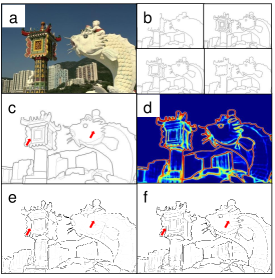
Figure 1: Illustration of the proposed Uncertainty-Aware Edge Detector (UAED). The first row shows (a) an image from the BSDS test set and (b) four diverse labels by different annotators. The second row shows (c) the final edge label computed by majority voting and (d) our estimated uncertainty map (red means high uncertainty and blue means low uncertainty). The third row shows the edge detection results by (e) EDTER [41] and (f) our UAED, both processed by non-maximum suppression.

Edge detection is a fundamental low-level vision task. It greatly reduces irrelevant information and retains the most important structural attributes. An efficient edge detector can generate structural edges that depict important areas from a whole image, thereby benefiting many downstream tasks [42, 63, 31, 37, 50]. Early pioneering methods [26, 4] compute the gradient and choose suitable thresholds to select pixels with obvious brightness changes. Hand-crafted feature based methods [35, 1] extract features from low-level cues including density and texture, and then design complex rules to distinguish edges. Benefiting from the powerful feature representation of Convolution Neural Network (CNN) and Transformer, recent works [59, 32, 16, 41] concentrate on designing elaborate network architectures to learn high-level semantic representations.

The previous efforts are mainly dedicated to designing advanced networks to extract distinctive features. Except for the well-designed models, precise pixel-level annotation is another key factor in building an efficient edge detector under the supervised setting. Due to the complexity of the scenes and the ambiguity of the edges, most of the works [1, 36] involve multiple annotators for labeling edges. However, the subjectivity of the annotators, e.g., different people may perceive the same scene differently and annotate the edges at different granularities, leading to inconsistent annotations (Fig. 1(b)). Previous methods simply utilize the majority voting strategy to fuse multiple annotations into single ground truth, where all annotations are averaged to generate an edge probability map (Fig. 1(c)), ranging from 0 to 1. During training, the pixels with probability higher than a fixed threshold are regarded as positive and the pixels with probability equal to 0 as negative. And the remaining pixels are dropped. Such a simple voting process neglects the inherent ambiguity and label bias caused by the labeling process.

To address the issues, in this paper, we propose a novel uncertainty-aware edge detection (UAED) framework that converts the deterministic labels into distributions to explore the inherent label ambiguity in the edge detection task. Unlike previous works that focus on architecture modification, we target modeling the uncertainty underlying the multiple edge annotations.

Specifically, the proposed UAED is designed based on the encoder-decoder architecture, where the encoder generates the feature representations followed by two separate decoders. Instead of using fixed labels, we treat the prediction as a learnable Gaussian distribution, whose mean and variance are learned by two decoders respectively, and the variance can be supervised by multiple annotations. The learned variance can be naturally regarded as uncertainty, which measures the label ambiguity. Therefore we further utilize the learned uncertainty to boost the performance. Fig. 1(d) shows the estimated uncertainty map. We can observe that the uncertainties of pixels that are close to edges are much higher than those of smooth regions. This phenomenon suggests that pixels with higher uncertainty are visually more important than pixels with lower uncertainty and can be regarded as hard samples for detecting edges. Thus inspired, unlike most uncertainty estimation methods that regard the pixels with higher uncertainty as unreliable and discard them, we encourage the model to learn more from the hard samples with higher uncertainty progressively. The experiments on two popular edge detection datasets with multiple annotations show the effectiveness of our proposed method. Compared with transformer-based EDTER [41] (Fig. 1(e)), our proposed UAED combined with CNN-based architecture can generate more detailed edges (Fig. 1(f)), while requires less computation resource and time. Our contributions can be summarized as follows:

• We propose an uncertainty-aware edge detector, named UAED, which captures the inherent ambiguity caused by multiple subjective annotations. To our best knowledge, this is the first work that provides an uncertainty perspective in edge detection.

• We concentrate on the pixels with higher uncertainty that play a more important role in edge detection, and further design an adaptive weighting loss to emphasize the training from those hard pixels.

• UAED can be combined with various encoder-decoder backbones without increasing much computation burden. We conduct comprehensive experiments on popular datasets across different model architectures and achieve consistent improvement.

2 Related Work

2.1 Edge Detection

Edge detection is an important vision task have been attracting a great amount of study. Early methods, such as Sobel [26] and Canny [4], calculate the gradient of density, color or texture of the images for edge clues. Traditional learning-based methods aim to design hand-crafted features from low-level density and texture cues to train a edge classifier. For example, Pb [35] defines the changes in brightness, color and texture as the edge features. gPb [1] utilizes standard Normalized Cuts for detecting edges.

Benefiting from the success of deep learning technologies, CNN-based methods become predominant edge detectors. Early methods [47, 3] are based on image patches that extract features from the predefined patches, and determine whether there are edge pixels. Later, pixel-based models have achieved promising performance. HED [59] utilizes VGG16 [49] as the backbone and obtains five stage feature maps as the side outputs, which are then fused into final outputs by learnable image-level weights. RCF [32] connects each convolution layer in VGG16 to a convolution layer, and then accumulate the results to attain hybrid features to fully use multi-scale multi-level information. LPCB [9] applies VGG16 as the backbone and utilizes the ResNetXt [17] block and deconv module to fuse features across stages to decode the edge maps. Instead of treating side outputs and final outputs the same, BDCN [16] approximates the specific edge ground truth for different scales. RINDNet [40] uses multi-branch strategy for fine grained edge detection. Recently, a transformer-based edge detector EDTER [41] is proposed, which first splits the input image into a sequence of $16\times 16$ patches to extract global features, and then extracts the short-range local cues on $8\times 8$ patches.

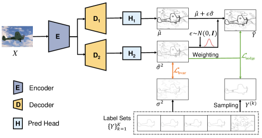
Figure 2: The overall framework of our proposed UAED. Given an input $X$, the encoder $\mathcal{E}$ extracts multi-scale features, which are then fed to two independent decoders $\mathcal{D}_{1},\mathcal{D}_{2}$ and prediction heads $\mathcal{H}_{1},\mathcal{H}_{2}$ to obtain respectively mean $\hat{\mu}$ and variance $\hat{\sigma}^{2}$. We construct a multi-variate Gaussian distribution according to the learned mean and variance, and sample prediction $\hat{Y}$ from this distribution. The learned variance is supervised by the label variance $\sigma^{2}$ computed from the labeling sets $\{Y^{(k)}\}_{k=1}^{K}$, and the prediction $\hat{Y}$ is supervised by the label $Y^{(k)}$ sampling from the labeling sets.

Some other works aim to construct lightweight models [51, 8] consuming as few resources as possible while maintaining performance. PiDiNet [51] introduces pixel difference convolution (PDC) which integrates the traditional edge detection operators such as Sobel and local binary patterns (LBP) into the popular convolution operations. LDC [8] is an encoder-decoder structure, where the encoder is tested on three different lightweight models, i.e., SqueezeNet [21], MobileNetV2 [18], and RegNetX [43]. The decoder module designs a spatially Squeeze-and-extraction (SSE) module to explore global contextual information and an SE module to extract local context.

Despite the thorough exploration of the network design and great performance achievement, existing works ignore the exploration of the inherent ambiguity in the label space, which is the focus of our work.

2.2 Uncertainty in Deep Learning

The major uncertainty encountered in deep learning [23] incorporates aleatoric (data) and epistemic (model) uncertainty, where data uncertainty is intrinsic while model uncertainty can be reduced by more data. Common methods for modeling uncertainty involve generative models [64, 27, 14], introducing new branches [5, 39], and regarding model parameters as a distribution [13, 30].

The techniques based on generative models can be classified into generative adversarial network (GAN) [64], energy-based model (EBM) [14, 66], variational autoencoder (VAE) [27, 2, 65], normalizing flow (NF) [29, 55], and a hybrid of the above methods [46, 53]. Introducing additional branches can operate on both the feature space [5] and label space [39] to convert the deterministic result into a distribution, such as Gaussian and Laplace distribution. Compared with other methods, modeling uncertainty on the parameters space is relatively time or memory consuming, such as MC-Dropout [13] and deep ensemble [30].

Despite effective uncertainty estimation methods having been successfully applied in many computer vision tasks, they have not been explored on the edge detection task. Our work is the first to model uncertainty in edge detection and design an efficient uncertainty estimation to explore the uncertainty underlying multiple edge labels.

3 Uncertainty-aware Edge Detection

The overview of the proposed uncertainty-aware edge detection (UAED) is shown in Fig. 2. Given an image $X\in\mathbb{R}^{H\times W\times 3}$ and its corresponding annotations $\{Y^{(k)}\}_{k=1}^{K}$, where $Y^{(k)}\in\mathbb{R}^{H\times W\times 1}$ is the $k\textrm{-th}$ annotation and $K$ is the number of annotations. We first feed $X$ into an encoder ($\mathcal{E}$) to extract multi-scale features, and then the extracted features are fed into two independent decoders ($\mathcal{D}_{1},\mathcal{D}_{2}$) and prediction heads ($\mathcal{H}_{1},\mathcal{H}_{2}$) to obtain mean ($\hat{\mu}$) and variance ($\hat{\sigma}^{2}$) for the learned Gaussian distribution respectively. The learned variance ($\hat{\sigma}^{2}$) is supervised by the variance computed from the label sets ($\sigma^{2}$). Finally, the sampling from the distribution is regarded as the prediction ($\hat{Y}$), which is supervised by the annotation $Y^{(k)}$ randomly sampled from the label sets.

We will detail the edge detection network in Section 3.1, and then introduce the proposed uncertainty estimation in Section 3.2 and the optimized objective in Section 3.3.

3.1 Edge Detection Network

We design our edge detector based on the encoder-decoder architecture, which is widely used in the edge detection task [8, 9, 7]. Here, we adopt EfficientNet [52] as the encoder and UNet++ [67] as the decoder. It should be noted that the edge detection network itself is not our contribution. So we do not pay more attention to the design of the network and just borrow the existing excellent framework for convenience. In fact, our proposed uncertainty-driven method can be combined with other edge detection networks, as demonstrated in the experiments in Section 4.6.

The encoder of our edge detection network consists of eight stages. Unlike the original EfficientNet starting with a convolutional layer that aims to change the input channels, we modify the stride of the first stage so that it can downsample the feature map by half. The seven middle stages are the same as the original EfficientNet, where each stage has different number of convolutional blocks consisting of the convolutional layer, batch normalization layer [22] and swish activation layer [44]. We remove the last ninth stage of the original EfficientNet [52] that is a classifier head including pooling and fully connected layers, since edge detection needs a fully convolutional network. We store the feature maps from the first, the third, the fourth, the sixth, and the eighth as multi-scale features for objects of different sizes, and then feed them into the following decoders. Note that the feature maps are down-sampled to $1/2$, $1/4$, $1/8$, $1/16$, and $1/32$ of the original images respectively. The details of the encoder are given in supplementary material.

The decoder of our edge detection network generates high-resolution representations from the received five-level multi-scale features by dense short-range connections and long-range connections, which is based on UNet++ [67] and can be viewed as four UNets with different sizes. Each UNet is a U-shape architecture including contracting and expansive path. The contracting path is responsible for the reduction of spatial information and the increase of abstract features. The expansive path up-samples the features and connects them with features from the contracting path to recover the images with high semantic information.

To summarize, for the input image $X$, we first extract the multi-scale features by the designed encoder. Then the extracted features are fed to the decoder and prediction head, which converts the high-dimensional channels of feature maps to one channel by a convolutional layer. Finally, a sigmoid activation function acts on the result to obtain the predicted edge map $\hat{Y}$, which ranges from 0 to 1.

3.2 Uncertainty Estimation

To introduce uncertainty into the edge detection task, we convert the deterministic output into a learnable distribution in the label space. Specifically, we add a decoder and a prediction head, which share the same structure but not the same parameters with the original decoder and prediction head, into the edge detection network. Then we feed the extracted multi-scale features into those two independent decoders ($\mathcal{D}_{1},\mathcal{D}_{2}$) and prediction heads ($\mathcal{H}_{1},\mathcal{H}_{2}$). The outputs are denoted as the mean $\hat{\mu}$ and the variance $\hat{\sigma}^{2}$ of the predicted edge maps:

$${\hat{\mu}}=\mathcal{H}_{1}(\mathcal{D}_{1}(\mathcal{E}(X)),\ \ \hat{\sigma}^{2}=\mathcal{H}_{2}(\mathcal{D}_{2}(\mathcal{E}(X))).$$ (1)

The predicted mean and variance are naturally built into a multi-variate Gaussian distribution, and the final prediction $\hat{Y}$ is sampled from the distribution by the reparameterization trick [25]:

$$\hat{Y}={\rm sigmoid}(\hat{\mu}+\epsilon\hat{\sigma}),\ \ \epsilon\sim\mathcal{N}(0,\text{I}).$$ (2)

3.3 Network Training

The optimization process of UAED contains two kinds of loss functions: balanced mean squared error (MSE) loss function for uncertainty estimation and weighted binary cross-entropy (BCE) loss function.

Balanced MSE loss for uncertainty estimation.

In addition to using a single available ground truth label, we hope to make full use of the entire candidate label sets. Thanks to multiple diverse annotations, we can compute the variance of the label sets ($\sigma^{2}$) as the supervision of the predicted variance ($\hat{\sigma}^{2}$), which can further be used to indicate the uncertainty estimation for the annotated labels. Therefore, we use $\mathcal{L}_{2}$ loss for estimating the variance defined as:

$$\mathcal{L}_{\rm var}=\sum_{j=1}^{HW}(\hat{\sigma}^{2}_{j}-\sigma^{2}_{j})^{2},$$ (3)

where $j$ denotes the $j$-th pixel in the estimated variance and ground truth variance map.

However, edge pixels are very sparse for no more than $10\%$ edge pixels in an image, so we use an adaptive weighting scheme to balance the loss, similar to  [19, 32]. The weight $\alpha$ for the positive samples is calculated as:

$$\alpha=|Y^{(k)}_{-}|\big{/}(|Y^{(k)}_{-}|+|Y^{(k)}_{+}|),$$ (4)

where $|\cdot|$ denotes the number of pixels, and $Y^{(k)}_{-}$ and $Y^{(k)}_{+}$ denote the negative and positive samples respectively in $k\textrm{-th}$ annotated edge map. Since the number of positive pixels is much smaller than that of negative ones, the balanced weight makes the model assign a higher weight to edge pixels. Denoting the weight for $Y_{j}$ as $M_{j}$, the balanced MSE loss is utilized to calculate the variance loss:

$$\mathcal{L}_{\rm bvar}=\sum_{j=1}^{HW}M_{j}(\hat{\sigma}^{2}_{j}-\sigma^{2}_{j})^{2},$$ (5)

where

$$M_{j}=\alpha Y_{j}+(1-\alpha)(1-Y_{j}).$$ (6)

Uncertainty-driven loss for edge detection.

Edge detection is a binary classification task, therefore the BCE loss is widely used in this task. Due to the imbalanced data, we add a balance weight similar to the variance loss. The balanced BCE loss can be denoted as:

$$\mathcal{L}_{\rm edge}=-\sum_{j=1}^{HW}M_{j}\Big{(} {Y^{(k)}_{j}}{\rm log}(\hat{Y}_{j})$$ (7)

$$+(1-{Y^{(k)}_{j}}){\rm log}(1-\hat{Y}_{j})\Big{)},$$

where $\hat{Y}_{j}$ and $Y_{j}^{(k)}$ are the $j$-th pixel of the prediction $\hat{Y}$ and label $Y^{(k)}$, respectively. The $k$-th label is randomly selected from the available label sets as the supervision signal.

Since the estimated variance ($\hat{\sigma}$) can be regarded as an indicator of the uncertainty of each pixel sample, it can be utilized to further guide the training of edge detector. Naturally, certain samples should be given higher weights while uncertain ones have low importance for training, which has been popularly used in many computer vision tasks [64]. Unfortunately, in our experiments, such a strategy can not boost the performance and, even worse, lead to an obvious performance drop (see the ablation study in Section 4.5). In fact, as shown in Fig. 1(d), we can observe that the pixels with higher uncertainty are usually close to the edges and boundaries in the estimated uncertainty map, which should not be neglected. Instead, those pixels should be prioritized in the training to enforce the model focus on learning from these difficult edges. Inspired by this observation, we design a different weighting strategy, where the pixels with higher uncertainty will be given large weights.

Besides, to prevent the pixels with higher uncertainty from confusing the model in the early training stage, we finally propose a progressive uncertainty-driven weighting strategy, where the pixels with higher uncertainty will be given larger weights progressively. The corresponding loss function is defined as:

$$\mathcal{L}_{\rm uedge}=\sum_{j=1}^{HW}{\rm{exp}}{(\beta_{t}\hat{\sigma}_{j})}\mathcal{L}_{\rm edge},$$ (8)

where $\beta_{t}=t/T$ denotes an adaptive factor, $t$ means the current epoch and $T$ means the total epochs. The final optimization objection is the sum of balanced MSE loss and weighted BCE loss:

$$\mathcal{L}=\mathcal{L}_{\rm uedge}+\mathcal{L}_{\rm bvar}.$$ (9)

4 Experiments

4.1 Datasets

We conduct experiments on two popular edge detection datasets, i.e., BSDS500 [1] and Multicue [36], which contain multiple annotations for each image.

Table 1: Results on the BSDS500 [1] testing set. SS is the single-scale testing, MS is the multi-scale testing, and VOC means training with extra PASCAL VOC data. The best two results are denoted as red and blue respectively, and the same for other tables.

Method	Backbone	Pub.’Year	SS			MS			SS-VOC			MS-VOC
			ODS	OIS	AP	ODS	OIS	AP	ODS	OIS	AP	ODS	OIS	AP
Canny [4]	-	PAMI’86	0.611	0.676	0.520	-	-	-	-	-	-	-	-	-
gPb-UCM [1]	-	PAMI’10	0.729	0.755	0.745	-	-	-	-	-	-	-	-	-
SCG [57]	-	NeurIPS’12	0.739	0.758	0.773	-	-	-	-	-	-	-	-	-
SE [10]	-	PAMI’14	0.743	0.764	0.800	-	-	-	-	-	-	-	-	-
OEF [15]	-	CVPR’15	0.746	0.770	0.815	-	-	-	-	-	-	-	-	-
DeepEdge [3]	AlexNet	CVPR’15	0.753	0.772	0.807	-	-	-	-	-	-	-	-	-
DeepContour [47]	AlexNet	CVPR’15	0.757	0.776	0.790	-	-	-	-	-	-	-	-	-
HED [59]	VGG16	ICCV’15	0.788	0.808	0.840	-	-	-	-	-	-	-	-	-
Deep Boundary [28]	VGG16	ICLR’15	0.789	0.811	0.789	0.803	0.820	0.848	0.809	0.827	0.861	0.813	0.831	0.866
CEDN [62]	VGG16	CVPR’16	0.788	0.804	-	-	-	-	-	-	-	-	-	-
RDS [33]	VGG16	CVPR’16	0.792	0.810	0.818	-	-	-	-	-	-	-	-	-
COB [34]	VGG16	ECCV’16	0.793	0.820	0.859	-	-	-	-	-	-	-	-	-
AMH-Net [60]	ResNet50	NeurIPS’17	0.798	0.829	0.869	-	-	-	-	-	-	-	-	-
RCF [32]	VGG16	CVPR’17	0.798	0.815	-	-	-	-	0.806	0.823	-	0.811	0.830	0.846
CED [54]	VGG16	CVPR’17	0.803	0.820	0.871	-	-	-	0.815	0.833	0.889	-	-	-
LPCB [9]	VGG16	ECCV’18	0.800	0.816	-	-	-	-	0.808	0.824	-	0.815	0.834	-
BDCN [16]	VGG16	CVPR’19	0.806	0.826	0.847	-	-	-	0.820	0.838	0.888	0.828	0.844	0.890
DSCD [7]	VGG16	ACMMM’20	0.802	0.817	-	-	-	-	0.813	0.836	-	0.822	0.859	-
LDC [8]	MobileNetV2	ACMMM’21	0.799	0.816	0.837	-	-	-	0.812	0.826	0.857	0.819	0.834	0.860
PiDiNet [51]	PDC	ICCV’21	-	-	-	-	-	-	0.807	0.823	-	-	-	-
FCL-Net [61]	VGG16	NN’22	0.807	0.822	-	0.816	0.833	-	0.815	0.834	-	0.826	0.845	-
EDTER [41]	Transformer	CVPR’22	0.824	0.841	0.880	0.840	0.858	0.896	0.832	0.847	0.886	0.848	0.865	0.903
UAED (Ours)	VGG16	-	0.808	0.827	0.872	0.819	0.838	0.881	0.820	0.840	0.889	0.830	0.850	0.895
	EfficientNet	-	0.829	0.847	0.892	0.837	0.855	0.897	0.838	0.855	0.902	0.844	0.864	0.905

BSDS500 contains 500 RGB natural images, of which 200 are for training, 100 for validation, and 200 for testing. Each image is manually annotated by 4-9 annotators. Data augmentation follows LPCB [9], which rotates each image at 25 different angles and selects the largest rectangle. Then each image is flipped (horizontally, vertically, and a combination of both) at each angle. So the scale of the training dataset has expanded by 100 times. Moreover, PASCAL VOC Context Dataset [12] with 10,103 images is used as the additional training data, whose edge annotations are obtained from the semantic masks by the Laplacian detector.

Multicue is composed of 100 scenes captured to study boundary and edge detection in challenging natural scenes. Each scene contains a left-view and a right-view short (10-frame) sequence, and the last frame of each left-view sequence is labeled with edges by six annotators and boundaries by five annotators. Data is augmented by rotating at four different angles (0, 90, 180, 270) and flipping. 80 images are randomly selected for training and the remaining 20 images are for testing. This process is repeated three times and the average scores of three independent trials are regarded as the final results.

4.2 Implementation Details

We use Pytorch [38] based image segmentation (SMP) neural network library [20] as the deep learning framework to implement UAED. All parameters are updated by Adam optimizer [24]. Our model is trained with batchsize 4. The weight decay is set to 5e-4, and the learning rate is 1e-4. To speed up the training process, we follow LPCB [9] to make all training samples the same size, so that we can train in a mini-batch way. For the BSDS dataset, we rotate the images to keep the same size with $321\times 481$. For the Multicue dataset, each image with size $720\times 1280$ is randomly cropped to $512\times 512$ patches for training.

The experiments are conducted on a single RTX 3090, and the training time of 15 epochs is about 19 hours for the BSDS dataset and 3 hours for the Multicue dataset. During the training process, the edge prediction is supervised by one randomly sampled annotation from the available label sets, and the uncertainty is supervised by the variance of the label sets. In the inference stage, we feed the test image into our UAED and obtain a predicted label distribution, and the final predicted edge map is generated by a stochastic sampling from the predicted distribution.

4.3 Evaluation Metric

In the experiment, we use the widely used metrics for measuring performance. The first one is referred to the optimal dataset scale (ODS) which employs a fixed threshold for all images in the dataset, which is also called Maximum F-measure (MF). The second metric is called optimal image scale (OIS) which selects the optimal threshold for each image. The third one is the Average Precision (AP). Before evaluation, following previous works [32, 41], the predicted edge maps are processed by non-maximum suppression, and the localization tolerance is set to 0.0075, which controls the maximum allowed distance in matches between the predicted edge results and the ground truth.

4.4 Comparison with State-of-the-art

In this section, we compare the performance of the proposed UAED with existing excellent edge detectors, including traditional detectors such as Canny [4], CNN-based detectors such as HED [59] and RCF [32], and transformer-based detector EDTER [41].

BSDS results. The results are summarized in Table 1. We can see that our proposed UAED outperforms other previous CNN-based methods. In the single scale setting, compared with the second best CNN-based method BDCN [16], we obtain a large performance gain by 2.3%, 2.1% and 4.5% in terms of ODS, OIS and AP. We also achieve ODS=0.844, OIS=0.864 and AP=0.905 under the MS-VOC setting, which also surpasses BDCN [16] by a large margin (1.6%, 2.0% and 1.5%). Compared with transformer-based EDTER [41], we still achieve the best performance and increase the scores by 0.5%, 0.6%, and 1.2% in ODS, OIS and AP metrics when testing on a single scale input. The results are only slightly lower than EDTER under multi-scale settings. The possible reason is that EDTER is learned in a patch-based manner, so the results are greatly improved when testing under the multi-scale setting. To show the results more intuitively, we give the Precision-Recall curve in Fig. 3. The visualization results for some challenging samples in the BSDS testing set are shown in Fig. 4. It is clear that our UAED can extract more detailed edges. Moreover, we conduct experiments based on the VGG16 [49] encoder since most of the CNN-based methods utilize it. The results show that we still surpass all CNN-based methods, which further verifies the effectiveness of UAED.

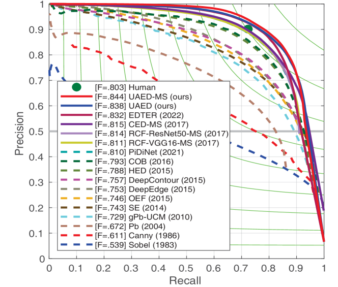
Figure 3: The precision-recall curves on BSDS500.

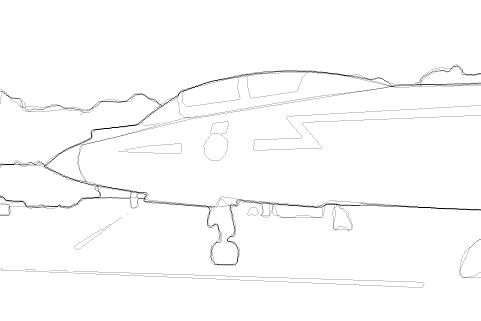
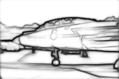
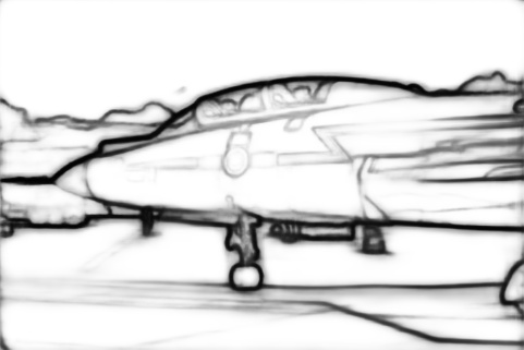
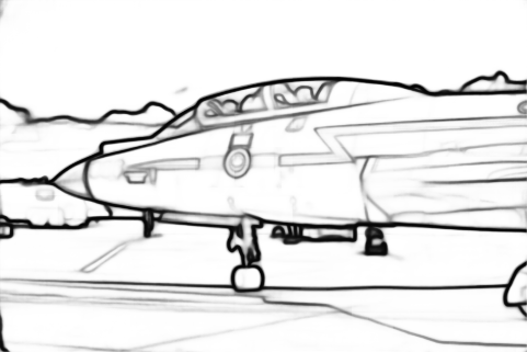
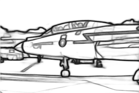
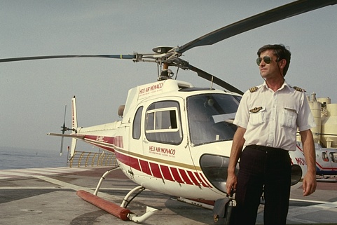
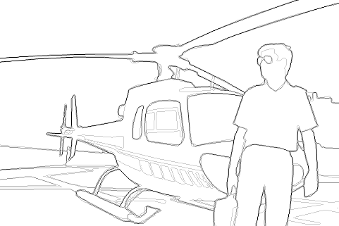
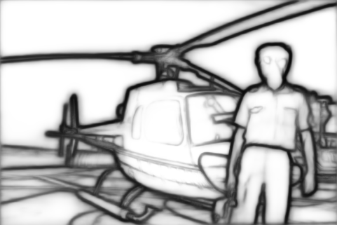
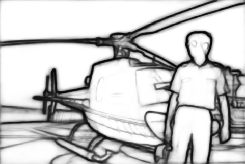
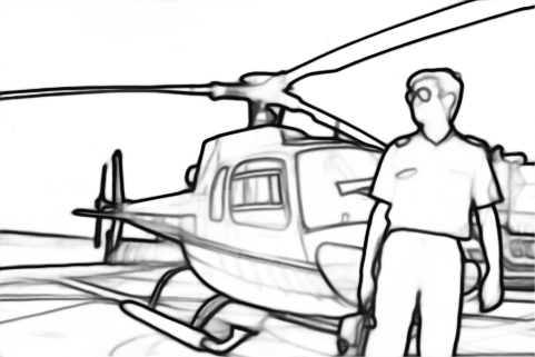
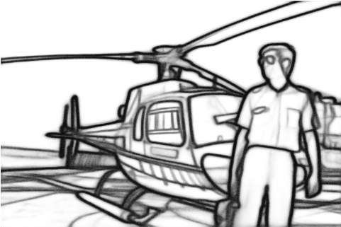
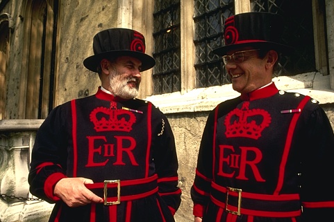
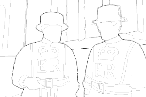
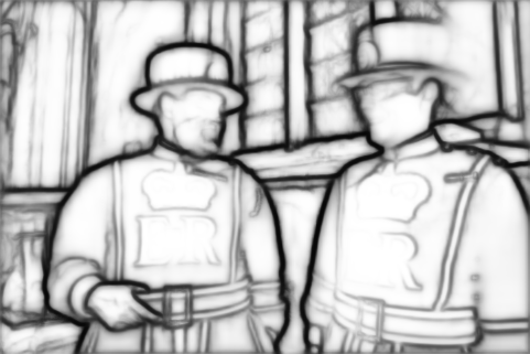
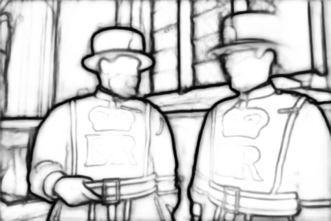
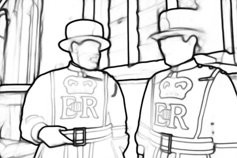
(a) Input	(b) Ground truth	(c) RCF [32]	(d) BDCN [16]	(e) EDTER [41]	(f) UAED(Ours)

Figure 4: Qualitative comparisons on three challenging samples in the BSDS500 test set.

Multicue results. Similarly, experiments are conducted on the Multicue edges and boundaries. The results are shown in Table 2. Our proposed UAED achieves a new state-of-the-art on the Multicue edge and boundary in three metrics (ODS=0.895, OIS=0.902, AP=0.949 in edge, and ODS=0.864, OIS=0.872, AP=0.927 in boundary).

Table 2: Comparisons on Multicue [36]. All results are obtained by a single scale input.

	Method	Pub.’Year	ODS	OIS	AP
Edge	Human [36]	VR’16	.750 (0.024)	-	-
	Multicue [36]	VR’16	.830 (0.002)	-	-
	HED [59]	ICCV’15	.851 (0.014)	.864 (0.011)	-
	RCF [32]	CVPR’17	.857 (0.004)	.862 (0.004)	-
	BDCN [16]	CVPR’19	.891 (0.001)	.898 (0.002)	.935(0.002)
	DSCD [7]	ACMMM’20	.871 (0.007)	.876 (0.002)	-
	LDC [8]	ACMMM’21	.881 (0.012)	.893 (0.011)	-
	PiDiNet [51]	ICCV’21	.855 (0.007)	.860 (0.005)	-
	FCL-Net [61]	NN’22	.875 (0.005)	.880 (0.005)	-
	EDTER [41]	CVPR’22	.894 (0.005)	.900 (0.003)	.944 (0.002)
	UAED (Ours)	-	.895 (0.002)	.902 (0.001)	.949 (0.002)
Boundary	Human [36]	VR’16	.760 (0.017)	-	-
	Multicue [36]	VR’16	.720 (0.014)	-	-
	HED [59]	ICCV’15	.814 (0.011)	.822 (0.008)	.869 (0.015)
	RCF [32]	CVPR’17	.817 (0.004)	.825 (0.005)	-
	BDCN [16]	CVPR’19	.836 (0.001)	.846 (0.003)	.893 (0.001)
	DSCD [7]	ACMMM’20	.828 (0.003)	.835 (0.004)	-
	LDC [8]	ACMMM’21	.839 (0.012)	.853 (0.006)	-
	PiDiNet [51]	ICCV’21	.818 (0.003)	.830 (0.005)	-
	FCL-Net [61]	NN’22	.834 (0.016)	.840 (0.016)	-
	EDTER [41]	CVPR’22	.861 (0.003)	.870 (0.004)	.919 (0.003)
	UAED (Ours)	-	.864 (0.004)	.872 (0.006)	.927 (0.006)

4.5 Ablation Study

There are several strategies influencing the performance, including adding a variance branch for uncertainty estimation (UE), supervising the estimation of variance by multiple annotations ($\mathcal{L}_{\rm bvar}$), and weighting BCE loss by estimated uncertainty ($\mathcal{L}_{\rm uedge}$). We conduct ablation studies on those aspects to explore the role of each part, and the results are shown in Table 3. All experiments are validated on the single scale with and without PASCAL VOC pre-training.

Table 3: The ablation study on the BSDS500 dataset for the role of every part plays. The results are obtained on a single scale input.

$\#$	Method	UE	$\mathcal{L}_{\rm bvar}$	$\mathcal{L}_{\rm uedge}$	ODS	OIS	AP
1	Baseline				0.824	0.841	0.875
2	UAED	✓			0.825	0.843	0.884
3		✓	✓		0.829	0.846	0.892
4		✓	✓	✓	0.829	0.847	0.892
5	Baseline-VOC				0.831	0.846	0.887
6	UAED-VOC	✓			0.834	0.852	0.895
7		✓	✓		0.836	0.853	0.901
8		✓	✓	✓	0.838	0.855	0.902

Experiments $\#1$ and $\#5$ are used as baseline methods, which fuse the multiple annotations into one single deterministic label according to a fixed threshold (0.3). The experiments ($\#2$-$\#4$ and $\#6$-$\#8$) are the results of our proposed UAED by deactivating different strategies which utilize all available multiple annotations.

The effect of the uncertainty estimation (UE). We first add a new decoder branch to the edge detector and convert the label space into a learnable distribution, which can be used to estimate uncertainty. Instead of generating deterministic predictions ($\#1$ and $\#5$), experiments ($\#2$ and $\#6$) regard the prediction as a distribution, and possess two independent decoders that represent mean and variance respectively. We can observe that experiment $\#2$ obtains 0.1%, 0.2%, and 0.9% in ODS, OIS, and AP than experiment $\#1$. Experiment $\#6$ obtains 0.3%, 0.6%, and 0.8% in ODS, OIS, and AP than experiment $\#5$. The improvements clearly show the effectiveness of introducing uncertainty.

The effect of $\mathcal{L}_{\rm bvar}$. If there is not any explicit supervision of the uncertainty, the learning process will not be easy. Fortunately, we can compute the variance from the provided label sets as the variance supervision ($\#3$ and $\#7$). From the ablations, we can see that experiment $\#3$ increases the score by 0.4% (ODS), 0.3% (OIS), and 0.8% (AP) than $\#2$. Similarly, experiment $\#7$ obtains 0.2% (ODS), 0.1% (OIS), and 0.6% (AP) than $\#6$. The improvements clearly show the benefit of this explicit supervision.

Table 4: The experiments of different weighting methods. All results are obtained by a single scale input.

Method	ODS	OIS	AP
$e^{-\hat{\sigma}}\mathcal{L}_{\rm edge}+2\hat{\sigma}$	0.825	0.843	0.884
$e^{\hat{\sigma}}\mathcal{L}_{\rm edge}$	0.826	0.846	0.891
$e^{\beta_{t}\sigma}\mathcal{L}_{\rm edge}$	0.826	0.845	0.890
$e^{\beta_{t}\hat{\sigma}}\mathcal{L}_{\rm edge}$	0.829	0.847	0.892

The effect of $\mathcal{L}_{\rm uedge}$. The progressive weighting loss makes the network first learn the variance as uncertainty, then utilize the learned uncertainty to progressively focus on the pixels with higher uncertainty. The experiments ($\#4$ and $\#8$) show that the weighting strategy can further improve performance.

The effect of different weighting loss. Instead of the traditional strategy (lower weight for higher uncertainty), we design a progressive weighting loss to emphasize the pixels with higher uncertainty. To verify this, we conduct ablation experiments shown in Table 4. Compared with other strategies, i.e. the traditional weighting loss (the first row), the fixed weighting loss (the second row), and the ground-truth label variance for weighting loss (the third row), our designed strategy achieves the best performance.

Table 5: The experiments on the BSDS500 dataset for different uncertainty estimation (UE) strategies. All results are obtained by a single scale input.

UE Type	UE Method	ODS	OIS	AP
-	Baseline	0.824	0.841	0.875
Epistemic (Model)	MC Dropout	0.825	0.842	0.882
	RBUE	0.825	0.843	0.882
Aleatoric (Data)	CVAE-based	0.821	0.844	0.880
	EBM-based	0.824	0.842	0.884
	Probabilistic Embedding	0.823	0.839	0.885
Data	UAED (Ours)	0.829	0.847	0.892

4.6 Further Analysis

Comparison with different uncertainty estimation methods. Uncertainty estimation is the most vital part of UAED, so we explore the influence of different methods. The popular uncertainty estimation methods include MC dropout [13], RBUE [56], CVAE-based [65], EBM-based [11], and probabilistic embedding [48]. MC Dropout [13] and RBUE [56] model epistemic (model) uncertainty, and both of them usually require hundreds of forwards to obtain excellent results. Generative model based methods, including CVAE-based and EBM-based models, learn low-level latent space, which captures randomness caused by the data.

Table 6: The experiments about different encoder and decoder structures. All results are obtained by a single scale input.

Encoder / Decoder	ODS	OIS	AP
VGG [49] / UNet++ [67]	0.801	0.820	0.862
+UAED	0.808(+.007)	0.827(+.007)	0.872(+.010)
EfficientNet [52]/UNet[45]	0.821	0.836	0.878
+UAED	0.824(+.003)	0.843(+.007)	0.886(+.008)
SegFormer [58] / UNet [45]	0.822	0.838	0.873
+UAED	0.828(+.006)	0.845(+.007)	0.888(+.015)

Probabilistic embedding builds distribution in the feature space while the proposed UAED differs in the label distribution, and both model aleatoric (data) uncertainty. The details of different uncertainty estimation methods can be found in the supplementary material.

Table 5 presents the comparison. MC dropout and RBUE only bring minor improvement and other methods are even inferior to baseline. By introducing the uncertainty to the label space, UAED obtains the best improvement.

The improvement for different backbones. Our proposed UAED is a play-and-plug module, so we combine it with diverse encoder-decoder architectures to verify its effectiveness. Specifically, the encoder contains CNN-based VGG [49], EfficientNet [52], and transformer-based SegFormer [58]. The decoder includes popular UNet [45] and UNet++ [67]. All encoders are pre-trained on the ImageNet [6] dataset. The results in Table 6 show a consistent performance gain of the proposed UAED, validating that UAED can be easily combined with the existing frameworks to boost performance consistently.

Computational cost. Our experiments are conducted on a single RTX 3090, which consume 12G GPU memory for the BSDS dataset with a batch size of 4. We also compute the inference time. The speed of our proposed UAED is 17 FPS, which increases not too much (19 FPS for the encoder-decoder baseline model). By comparison, the transformer-based EDTER [41] consumes 15G GPU (stage I) and 14G (stage II) with batchsize of 1 for training and runs at 5 FPS for inference. The statistics indicate that our proposed UAED obtains a comparable performance only using relatively less time and resources.

5 Conclusion

We are the first work to employ uncertainty into the edge detector to model the inherent ambiguity underlying multiple annotations. The uncertainty-aware edge detector (UAED) regards the label space as the distribution and adds a branch to estimate the variance, which can be further utilized to progressively weight the optimized loss function. We conduct experiments on BSDS and Multicue datasets. The results demonstrate that our proposed UAED can bring consistent improvement by exploring the uncertainty beneath the multiple annotations.

Limitation. This method still needs labor-consuming pixel-level annotations. How to utilize fewer annotations to achieve competitive results remains an open issue.

Acknowledgements. This work is supported by National Natural Science Foundation of China (62271042) and Beijing Natural Science Foundation (M22022, L211015).

References

- [1] Pablo Arbelaez, Michael Maire, Charless Fowlkes, and Jitendra Malik. Contour detection and hierarchical image segmentation. IEEE Trans. Pattern Anal. Mach. Intell., 33(5):898–916, 2010.
- [2] Christian F Baumgartner, Kerem C Tezcan, Krishna Chaitanya, Andreas M Hötker, Urs J Muehlematter, Khoschy Schawkat, Anton S Becker, Olivio Donati, and Ender Konukoglu. Phiseg: Capturing uncertainty in medical image segmentation. In International Conference on Medical Image Computing and Computer-Assisted Intervention, pages 119–127. Springer, 2019.
- [3] Gedas Bertasius, Jianbo Shi, and Lorenzo Torresani. Deepedge: A multi-scale bifurcated deep network for top-down contour detection. In IEEE Conf. Comput. Vis. Pattern Recog., pages 4380–4389, 2015.
- [4] John Canny. A computational approach to edge detection. IEEE Trans. Pattern Anal. Mach. Intell., (6):679–698, 1986.
- [5] Jie Chang, Zhonghao Lan, Changmao Cheng, and Yichen Wei. Data uncertainty learning in face recognition. In IEEE Conf. Comput. Vis. Pattern Recog., pages 5710–5719, 2020.
- [6] Jia Deng, Wei Dong, Richard Socher, Li-Jia Li, Kai Li, and Li Fei-Fei. Imagenet: A large-scale hierarchical image database. In IEEE Conf. Comput. Vis. Pattern Recog., pages 248–255. Ieee, 2009.
- [7] Ruoxi Deng and Shengjun Liu. Deep structural contour detection. In ACM Int. Conf. Multimedia, pages 304–312, 2020.
- [8] Ruoxi Deng, Shengjun Liu, Jinxin Wang, Huibing Wang, Hanli Zhao, and Xiaoqin Zhang. Learning to decode contextual information for efficient contour detection. In ACM Int. Conf. Multimedia, pages 4435–4443, 2021.
- [9] Ruoxi Deng, Chunhua Shen, Shengjun Liu, Huibing Wang, and Xinru Liu. Learning to predict crisp boundaries. In Eur. Conf. Comput. Vis., pages 562–578, 2018.
- [10] Piotr Dollár and C Lawrence Zitnick. Fast edge detection using structured forests. IEEE Trans. Pattern Anal. Mach. Intell., 37(8):1558–1570, 2014.
- [11] Yilun Du and Igor Mordatch. Implicit generation and generalization in energy-based models. arXiv preprint arXiv:1903.08689, 2019.
- [12] Mark Everingham, Luc Van Gool, Christopher KI Williams, John Winn, and Andrew Zisserman. The pascal visual object classes (voc) challenge. Int. J. Comput. Vis., 88(2):303–338, 2010.
- [13] Yarin Gal and Zoubin Ghahramani. Dropout as a bayesian approximation: Representing model uncertainty in deep learning. In international conference on machine learning, pages 1050–1059. PMLR, 2016.
- [14] Fredrik K Gustafsson, Martin Danelljan, Goutam Bhat, and Thomas B Schön. Energy-based models for deep probabilistic regression. In Eur. Conf. Comput. Vis., pages 325–343. Springer, 2020.
- [15] Sam Hallman and Charless C Fowlkes. Oriented edge forests for boundary detection. In IEEE Conf. Comput. Vis. Pattern Recog., pages 1732–1740, 2015.
- [16] Jianzhong He, Shiliang Zhang, Ming Yang, Yanhu Shan, and Tiejun Huang. Bi-directional cascade network for perceptual edge detection. In IEEE Conf. Comput. Vis. Pattern Recog., pages 3828–3837, 2019.
- [17] Kaiming He, Xiangyu Zhang, Shaoqing Ren, and Jian Sun. Deep residual learning for image recognition. In IEEE Conf. Comput. Vis. Pattern Recog., pages 770–778, 2016.
- [18] Andrew Howard, Andrey Zhmoginov, Liang-Chieh Chen, Mark Sandler, and Menglong Zhu. Inverted residuals and linear bottlenecks: Mobile networks for classification, detection and segmentation. 2018.
- [19] Jyh-Jing Hwang and Tyng-Luh Liu. Contour detection using cost-sensitive convolutional neural networks. arXiv preprint arXiv:1412.6857, 2014.
- [20] Pavel Iakubovskii. Segmentation models pytorch. https://github.com/qubvel/segmentation_models.pytorch, 2019.
- [21] Forrest N Iandola, Song Han, Matthew W Moskewicz, Khalid Ashraf, William J Dally, and Kurt Keutzer. Squeezenet: Alexnet-level accuracy with 50x fewer parameters and¡ 0.5 mb model size. arXiv preprint arXiv:1602.07360, 2016.
- [22] Sergey Ioffe and Christian Szegedy. Batch normalization: Accelerating deep network training by reducing internal covariate shift. In International conference on machine learning, pages 448–456. PMLR, 2015.
- [23] Alex Kendall and Yarin Gal. What uncertainties do we need in bayesian deep learning for computer vision? Adv. Neural Inform. Process. Syst., 30, 2017.
- [24] Diederik P Kingma and Jimmy Ba. Adam: A method for stochastic optimization. arXiv preprint arXiv:1412.6980, 2014.
- [25] Durk P Kingma, Tim Salimans, and Max Welling. Variational dropout and the local reparameterization trick. Adv. Neural Inform. Process. Syst., 28, 2015.
- [26] Josef Kittler. On the accuracy of the sobel edge detector. Image and Vision Computing, 1(1):37–42, 1983.
- [27] Simon Kohl, Bernardino Romera-Paredes, Clemens Meyer, Jeffrey De Fauw, Joseph R Ledsam, Klaus Maier-Hein, SM Eslami, Danilo Jimenez Rezende, and Olaf Ronneberger. A probabilistic u-net for segmentation of ambiguous images. Adv. Neural Inform. Process. Syst., 31, 2018.
- [28] Iasonas Kokkinos. Pushing the boundaries of boundary detection using deep learning. Int. Conf. Learn. Represent., 2016.
- [29] Manoj Kumar, Mohammad Babaeizadeh, Dumitru Erhan, Chelsea Finn, Sergey Levine, Laurent Dinh, and Durk Kingma. Videoflow: A conditional flow-based model for stochastic video generation. arXiv preprint arXiv:1903.01434, 2019.
- [30] Balaji Lakshminarayanan, Alexander Pritzel, and Charles Blundell. Simple and scalable predictive uncertainty estimation using deep ensembles. Adv. Neural Inform. Process. Syst., 30, 2017.
- [31] Jiang-Jiang Liu, Qibin Hou, and Ming-Ming Cheng. Dynamic feature integration for simultaneous detection of salient object, edge, and skeleton. IEEE Trans. Image Process., 29:8652–8667, 2020.
- [32] Yun Liu, Ming-Ming Cheng, Xiaowei Hu, Kai Wang, and Xiang Bai. Richer convolutional features for edge detection. In IEEE Conf. Comput. Vis. Pattern Recog., pages 3000–3009, 2017.
- [33] Yu Liu and Michael S Lew. Learning relaxed deep supervision for better edge detection. In IEEE Conf. Comput. Vis. Pattern Recog., pages 231–240, 2016.
- [34] Kevis-Kokitsi Maninis, Jordi Pont-Tuset, Pablo Arbeláez, and Luc Van Gool. Convolutional oriented boundaries. In Eur. Conf. Comput. Vis., pages 580–596. Springer, 2016.
- [35] David R Martin, Charless C Fowlkes, and Jitendra Malik. Learning to detect natural image boundaries using local brightness, color, and texture cues. IEEE Trans. Pattern Anal. Mach. Intell., 26(5):530–549, 2004.
- [36] David A Mély, Junkyung Kim, Mason McGill, Yuliang Guo, and Thomas Serre. A systematic comparison between visual cues for boundary detection. Vision research, 120:93–107, 2016.
- [37] Kamyar Nazeri, Eric Ng, Tony Joseph, Faisal Qureshi, and Mehran Ebrahimi. Edgeconnect: Structure guided image inpainting using edge prediction. In IEEE Conf. Comput. Vis. Pattern Recog. Worksh., pages 0–0, 2019.
- [38] Adam Paszke, Sam Gross, Soumith Chintala, Gregory Chanan, Edward Yang, Zachary DeVito, Zeming Lin, Alban Desmaison, Luca Antiga, and Adam Lerer. Automatic differentiation in pytorch. 2017.
- [39] Badri N Patro, Mayank Lunayach, Shivansh Patel, and Vinay P Namboodiri. U-cam: Visual explanation using uncertainty based class activation maps. In Int. Conf. Comput. Vis., pages 7444–7453, 2019.
- [40] Mengyang Pu, Yaping Huang, Qingji Guan, and Haibin Ling. Rindnet: Edge detection for discontinuity in reflectance, illumination, normal and depth. In Int. Conf. Comput. Vis., pages 6879–6888, 2021.
- [41] Mengyang Pu, Yaping Huang, Yuming Liu, Qingji Guan, and Haibin Ling. Edter: Edge detection with transformer. In IEEE Conf. Comput. Vis. Pattern Recog., pages 1402–1412, 2022.
- [42] Xuebin Qin, Zichen Zhang, Chenyang Huang, Chao Gao, Masood Dehghan, and Martin Jagersand. Basnet: Boundary-aware salient object detection. In IEEE Conf. Comput. Vis. Pattern Recog., pages 7479–7489, 2019.
- [43] Ilija Radosavovic, Raj Prateek Kosaraju, Ross Girshick, Kaiming He, and Piotr Dollár. Designing network design spaces. In IEEE Conf. Comput. Vis. Pattern Recog., pages 10428–10436, 2020.
- [44] Prajit Ramachandran, Barret Zoph, and Quoc V Le. Swish: a self-gated activation function. arXiv preprint arXiv:1710.05941, 7(1):5, 2017.
- [45] Olaf Ronneberger, Philipp Fischer, and Thomas Brox. U-net: Convolutional networks for biomedical image segmentation. In International Conference on Medical image computing and computer-assisted intervention, pages 234–241. Springer, 2015.
- [46] Raghavendra Selvan, Frederik Faye, Jon Middleton, and Akshay Pai. Uncertainty quantification in medical image segmentation with normalizing flows. In International Workshop on Machine Learning in Medical Imaging, pages 80–90. Springer, 2020.
- [47] Wei Shen, Xinggang Wang, Yan Wang, Xiang Bai, and Zhijiang Zhang. Deepcontour: A deep convolutional feature learned by positive-sharing loss for contour detection. In IEEE Conf. Comput. Vis. Pattern Recog., pages 3982–3991, 2015.
- [48] Yichun Shi and Anil K Jain. Probabilistic face embeddings. In Int. Conf. Comput. Vis., pages 6902–6911, 2019.
- [49] Karen Simonyan and Andrew Zisserman. Very deep convolutional networks for large-scale image recognition. arXiv preprint arXiv:1409.1556, 2014.
- [50] Xiao Song, Xu Zhao, Hanwen Hu, and Liangji Fang. Edgestereo: A context integrated residual pyramid network for stereo matching. In ACCV, pages 20–35. Springer, 2018.
- [51] Zhuo Su, Wenzhe Liu, Zitong Yu, Dewen Hu, Qing Liao, Qi Tian, Matti Pietikäinen, and Li Liu. Pixel difference networks for efficient edge detection. pages 5117–5127, 2021.
- [52] Mingxing Tan and Quoc Le. Efficientnet: Rethinking model scaling for convolutional neural networks. In International conference on machine learning, pages 6105–6114. PMLR, 2019.
- [53] MM Valiuddin, Christiaan GA Viviers, Ruud JG van Sloun, Fons van der Sommen, et al. Improving aleatoric uncertainty quantification in multi-annotated medical image segmentation with normalizing flows. In Uncertainty for Safe Utilization of Machine Learning in Medical Imaging, and Perinatal Imaging, Placental and Preterm Image Analysis, pages 75–88. Springer, 2021.
- [54] Yupei Wang, Xin Zhao, and Kaiqi Huang. Deep crisp boundaries. In IEEE Conf. Comput. Vis. Pattern Recog., pages 3892–3900, 2017.
- [55] Tom Wehrbein, Marco Rudolph, Bodo Rosenhahn, and Bastian Wandt. Probabilistic monocular 3d human pose estimation with normalizing flows. In Int. Conf. Comput. Vis., pages 11199–11208, 2021.
- [56] Yufeng Xia, Jun Zhang, Zhiqiang Gong, Tingsong Jiang, and Wen Yao. Rbue: A relu-based uncertainty estimation method of deep neural networks. arXiv preprint arXiv:2107.07197, 2021.
- [57] Ren Xiaofeng and Liefeng Bo. Discriminatively trained sparse code gradients for contour detection. Adv. Neural Inform. Process. Syst., 25, 2012.
- [58] Enze Xie, Wenhai Wang, Zhiding Yu, Anima Anandkumar, Jose M Alvarez, and Ping Luo. Segformer: Simple and efficient design for semantic segmentation with transformers. Adv. Neural Inform. Process. Syst., 34:12077–12090, 2021.
- [59] Saining Xie and Zhuowen Tu. Holistically-nested edge detection. In Int. Conf. Comput. Vis., pages 1395–1403, 2015.
- [60] Dan Xu, Wanli Ouyang, Xavier Alameda-Pineda, Elisa Ricci, Xiaogang Wang, and Nicu Sebe. Learning deep structured multi-scale features using attention-gated crfs for contour prediction. In Adv. Neural Inform. Process. Syst., pages 3961–3970, 2017.
- [61] Wenjie Xuan, Shaoli Huang, Juhua Liu, and Bo Du. Fcl-net: Towards accurate edge detection via fine-scale corrective learning. Neural Networks, 145:248–259, 2022.
- [62] Jimei Yang, Brian Price, Scott Cohen, Honglak Lee, and Ming-Hsuan Yang. Object contour detection with a fully convolutional encoder-decoder network. In IEEE Conf. Comput. Vis. Pattern Recog., pages 193–202, 2016.
- [63] Zhiding Yu, Rui Huang, Wonmin Byeon, Sifei Liu, Guilin Liu, Thomas Breuel, Anima Anandkumar, and Jan Kautz. Coupled segmentation and edge learning via dynamic graph propagation. Adv. Neural Inform. Process. Syst., 34:4919–4932, 2021.
- [64] Jing Zhang, Yuchao Dai, Mochu Xiang, Deng-Ping Fan, Peyman Moghadam, Mingyi He, Christian Walder, Kaihao Zhang, Mehrtash Harandi, and Nick Barnes. Dense uncertainty estimation. arXiv preprint arXiv:2110.06427, 2021.
- [65] Jing Zhang, Deng-Ping Fan, Yuchao Dai, Saeed Anwar, Fatemeh Sadat Saleh, Tong Zhang, and Nick Barnes. Uc-net: Uncertainty inspired rgb-d saliency detection via conditional variational autoencoders. In IEEE Conf. Comput. Vis. Pattern Recog., pages 8582–8591, 2020.
- [66] Jing Zhang, Jianwen Xie, Nick Barnes, and Ping Li. Learning generative vision transformer with energy-based latent space for saliency prediction. Adv. Neural Inform. Process. Syst., 34:15448–15463, 2021.
- [67] Zongwei Zhou, Md Mahfuzur Rahman Siddiquee, Nima Tajbakhsh, and Jianming Liang. Unet++: A nested u-net architecture for medical image segmentation. In Deep learning in medical image analysis and multimodal learning for clinical decision support, pages 3–11. Springer, 2018.