Efficient and scalable hybrid fluid-particle simulations with geometrically resolved particles on heterogeneous CPU-GPU architectures

Abstract

In recent years, it has become increasingly popular to accelerate numerical simulations using Graphics Processing Unit (GPU) s. In multiphysics simulations, the various combined methodologies may have distinctly different computational characteristics. Therefore, the best-suited hardware architecture can differ between the simulation components. Furthermore, not all coupled software frameworks may support all hardware. These issues predestinate or even force hybrid implementations, i.e., different simulation components running on different hardware. We introduce a hybrid coupled fluid-particle implementation with geometrically resolved particles. The simulation utilizes GPU s for the fluid dynamics, whereas the particle simulation runs on Central Processing Unit (CPU) s. We examine the performance of two contrasting cases of a fluidized bed simulation on a heterogeneous supercomputer. The hybrid overhead (i.e., the CPU-GPU communication) is negligible. The fluid simulation shows good performance utilizing nearly the entire memory bandwidth. Still, the GPU run time accounts for most of the total time. The parallel efficiency in a weak scaling benchmark for 1024 A100 GPU s is up to 71%. Frequent CPU-CPU communications occurring in the particle simulation are the leading cause of the decrease in parallel efficiency. The results show that hybrid implementations are promising for large-scale multiphysics simulations on heterogeneous supercomputers.

1 Introduction

Numerical multiphysics simulations are a powerful technique for conducting in-depth investigations of complex physical phenomena by providing detailed data, which is challenging, if not impossible, to collect in experiments. A prominent example is coupled fluid-particle simulations with geometrically resolved particles. Such simulations have been used in the literature to understand the formation and dynamics of dunes in river beds [1, 2, 3], investigate the erosion kinetics of soil under an impinging jet [4] and to analyze mobile sediment beds [5, 6]. A significant challenge with these simulations is that they are very computationally expensive, which is why they often run on supercomputers. Especially supercomputers containing Graphics Processing Unit (GPU) s have become increasingly popular in recent years [7, 8, 9] as they offer unprecedented computing power.
In such multiphysics simulations, the various combined methodologies may exhibit distinctly contrasting computational properties, e.g., problem sizes, parallel and sequential portions, frequency of conditions, and branching. Therefore, the best-suited hardware architecture can differ between the simulation components. Furthermore, there are practical reasons that can challenge multiphysics simulations: not all coupled software frameworks and modules may support the same hardware. We face these challenges in coupled fluid-particle simulations with geometrically resolved particles. The fluid simulation using a structured, grid-based methodology is ideally suited for GPU parallelization [10]. The situation is different for the particle simulation because it operates on unstructured data structures with irregular accesses due to frequent branching. On top of that, when combining the particle simulation with a fluid simulation using a fully resolved coupling, the number of particles is typically at least three orders of magnitude smaller than the number of fluid cells, leading to an imbalance of the workload. These characteristics of the particle simulation do not predestine it for GPU s. Porting the entire fluid-particle simulations from the Central Processing Unit (CPU) to the GPU would be an enormous expenditure of time. Latter is hard to justify for the particle simulation as it is debatable if the computational properties of the particle simulation are suited for GPU s at all. This is a major reason why coupled fluid-particle implementations still are often limited to CPU s [1, 3, 5], even though GPU s would be best suited for the dominating part: the fluid simulation. These issues predestinate or even force a hybrid implementation, i.e., utilizing GPU s for the fluid dynamics and the coupling. In contrast, the Particle Dynamics (PD) simulation runs on CPU s.
Hybrid coupled fluid-particle simulations have been used several times in the literature. On the one hand, a common approach is to use the CPU for the fluid simulation and the GPU for the PD, for example, when simulating deformable bodies (using the finite element method) in a fluid, i.e., blood cells in cellular blood flow [11]. Here, the focus is more on structural mechanics, as the finite element method dominates the overall run time. The latter approach has also been taken in the literature to couple commercial Computational Fluid Dynamics (CFD) solvers on the CPU such as Ansys [12, 13], or AVL fire [14] with the Discrete Element Method (DEM) on the GPU. This approach also appears in the context of fluidized beds [15, 16]. On the other hand, several publications have used the approach promising for our problem: using the CPU for the particles and the GPU for the fluid. One variant is to run the Lattice Boltzmann Method (LBM) on a single GPU and use a single CPU for the particles [17], or use the GPU for both the fluid and the particles, but the CPU supports the particle dynamics through collision detection [18]. Another idea is to use either multiple CPU s for the particle simulation [19], or multiple GPU s for the LBM [20].
The Top500 list reports the most powerful supercomputer worldwide. The number of heterogeneous supercomputers, i.e., systems with additional accelerators such as GPU s, in the Top500 list has steadily increased in the last years, accounting for roughly 28% at the end of 2019 [21]. Each node of such a heterogeneous supercomputer typically consists of multiple CPU s and multiple GPU s [22]. On the one hand, hybrid implementation can fully utilize the capacities of a heterogeneous supercomputer by using both the CPU s and the GPU s. On the other hand, for a responsible use of a heterogeneous supercomputer, the performance has to meet specific criteria. First, the penalty introduced by the hybrid implementation (i.e., the CPU-GPU communication) has to be negligible compared to the overall run time. Second, the performance-critical fluid simulation should show good performance, i.e., fully utilize the GPU memory bandwidth. Third, the share of the GPU run time in the total run time must be sufficiently high to justify using a heterogeneous cluster. Fourth, it has to show a satisfactory weak scaling performance for the responsible use of multiple supercomputer nodes. However, none of the above publications provide a framework for geometrically resolved fluid-particle simulations fulfilling all the criteria.
In this paper, we want to investigate if hybrid implementations are suitable for large-scale coupled fluid-particle simulations on heterogeneous supercomputers. Therefore, we supplement the existing literature by introducing a multi-CPU-multi-GPU hybrid implementation for coupled fluid-particle simulations with geometrically resolved particles. To evaluate our implementation based on the above criteria, we provide in-depth performance analysis on a state-of-the-art heterogeneous supercomputer comparing two cases of a fluidized bed simulation with a distinctly different number of particles per volume. We assess the hybrid penalty, investigate the run time distribution among the various simulation components and provide an in-depth analysis of the weak scaling performance for up to 1024 A100 GPU s. We use code generation technologies to obtain highly efficient compute kernels and combine them with handwritten codes.
The paper starts in Section 2 with an introduction of the numerical methods, i.e., the LBM, the DEM, and the corresponding coupling. The numerical methods are followed by Section 3 with a description of the implementation. In Section 4, we provide a detailed performance examination. This examination includes the CPU-GPU communication overhead, the DEM performance, the run times of the different simulation components, a weak scaling, a roofline model, and an estimation of the hybrid speedup. The paper concludes with Section 5.

2 Numerical methods

Generally, fully resolved coupled fluid-particle simulations consist of three components: fluid dynamics, particle physics, and fluid-particle coupling. In this section, we introduce the background of the here applied methods based on the work of Rettinger et al. [23, 24]. Fig. 1 illustrates coupled fluid-particle simulations using the Partially Saturated Cells Method (PSM), which will be explained in the upcoming sections.

Figure 1: Two-dimensional sketch of coupled fluid-particle simulations using the PSM.

2.1 Lattice Boltzmann method

We use the LBM with the D3Q19 lattice model for the hydrodynamics simulation, an alternative to conventional Navier-Stokes solvers [25]. We evolve 19 Particle Distribution Functions (PDFs) $f_{q}$ with $q\in\{0,\ldots,18\}$ for every cell of a three-dimensional cartesian lattice. Each $f_{q}$ is associated with a lattice velocity $\boldsymbol{c}_{q}$. The underlying update rule is based on the Boltzmann equation, typically split into the streaming and collision steps. The cell-local collision relaxes the PDFs towards a thermodynamic equilibrium. The streaming propagates the post-collision PDFs $\widetilde{f_{q}}$ to neighboring cells. The collision step for the lattice cell $\boldsymbol{x}$ at time step $t$ is defined as

$$\widetilde{f_{q}}(\boldsymbol{x},t)=f_{q}(\boldsymbol{x},t)+C_{q}(\boldsymbol{x},t)+F_{q}(\boldsymbol{x},t),$$ (1)

with $C_{q}$ being the collision operator and $F_{q}$ the forcing operator. The streaming step

$$f_{q}(\boldsymbol{x}+\boldsymbol{c}_{q}\varDelta t,t+\varDelta t)=\widetilde{f_{q}}(\boldsymbol{x},t)$$ (2)

distributes the PDFs to neighboring cells. $\varDelta t$ is the time step size, which is typically 1 in the context of the LBM. The most commonly applied collision operator is based on the Single Relaxation Time (SRT) model (also known as the BGK model [26]). It relaxes the PDFs towards their equilibrium using a single relaxation time $\tau$:

$$C_{q}^{\text{SRT}}(\boldsymbol{x},t)=\frac{\varDelta t}{\tau}(f_{q}^{\text{eq}}(\rho_{\text{f}},\boldsymbol{U}_{\text{f}})-f_{q}(\boldsymbol{x},t)).$$ (3)

The relaxation time $\tau$ is linked to the kinematic fluid viscosity $\nu$ by:

$$\nu=(\tau-\varDelta t/2)c_{\text{s}}^{2}.$$ (4)

The equilibrium is defined as

$$f_{q}^{\text{eq}}(\rho_{\text{f}},\boldsymbol{U}_{\text{f}})=w_{q}\left(\rho_{\text{f}}+\rho_{0}\left(\frac{\boldsymbol{c}_{q}\cdot\boldsymbol{U}_{\text{f}}}{c_{\text{s}}^{2}}+\frac{{(\boldsymbol{c}_{q}\cdot\boldsymbol{U}_{\text{f}})}^{2}}{2c_{\text{s}}^{4}}-\frac{\boldsymbol{U}_{\text{f}}\cdot\boldsymbol{U}_{\text{f}}}{2c_{\text{s}}^{2}}\right)\right)$$ (5)

for incompressible flows [27] with $\rho_{0}=1$ and the lattice speed of sound $c_{\text{s}}=1/\sqrt{3}$. The cell-local quantities

$$\rho_{\text{f}}(\boldsymbol{x},t)=\sum_{q}f_{q}(\boldsymbol{x},t)\qquad\text{and}\qquad\boldsymbol{U}_{\text{f}}(\boldsymbol{x},t)=\frac{1}{\rho_{0}}\sum_{q}f_{q}(\boldsymbol{x},t)\boldsymbol{c}_{q}+\frac{\varDelta t}{2\rho_{0}}\boldsymbol{f}^{\text{ext}}$$ (6)

are calculated based on the moments of the PDFs. The forcing operator

$$F_{q}(\boldsymbol{x},t)=\varDelta tw_{q}\left[\frac{\boldsymbol{c}_{q}-\boldsymbol{U}_{\text{f}}}{c_{\text{s}}^{2}}+\frac{\boldsymbol{c}_{q}\cdot\boldsymbol{U}_{\text{f}}}{c_{\text{s}}^{4}}\cdot\boldsymbol{c}_{q}\right]\cdot\boldsymbol{f}^{\text{ext}}$$ (7)

incorporates external forces using the constant force density $\boldsymbol{f}^{\text{ext}}$ [28].

2.2 Particle dynamics

The total force $\boldsymbol{F}_{\text{p},i}$ acting on a particle $i$ consists of the following components:

$$\boldsymbol{F}_{\text{p},i}=\boldsymbol{F}_{\text{p},i}^{\text{col}}+\boldsymbol{F}_{\text{p},i}^{\text{hyd}}+\boldsymbol{F}_{\text{p},i}^{\text{ext}}.$$ (8)

In addition to the hydrodynamic force $\boldsymbol{F}_{\text{p},i}^{\text{hyd}}$ and external forces $\boldsymbol{F}_{\text{p},i}^{\text{ext}}$ (e.g., gravity), the particle interactions exert forces $\boldsymbol{F}_{\text{p},i}^{\text{col}}$ on each other due to collisions. The equations of motion have to be integrated to simulate the particle movements.

2.2.1 Particle interactions using the discrete element method

The collision between particle $i$ and $j$ is modeled using the DEM [29]. The collision force $\boldsymbol{F}_{\text{p},i}^{\text{col}}$ and torque $\boldsymbol{T}_{\text{p},i}^{\text{col}}$ on particle $i$ are computed as

$$\boldsymbol{F}_{\text{p},i}^{\text{col}}=\sum_{j,j\neq i}(\boldsymbol{F}_{ij,\text{n}}^{\text{col}}+\boldsymbol{F}_{ij,\text{t}}^{\text{col}}),$$ (9)

$$\boldsymbol{T}_{\text{p},i}^{\text{col}}=\sum_{j,j\neq i}(\boldsymbol{x}_{ij}^{\text{cp}}-\boldsymbol{x}_{\text{p},i})\times\boldsymbol{F}_{ij,\text{t}}^{\text{col}},$$ (10)

where the normal part of the collision force $\boldsymbol{F}_{ij,\text{n}}^{\text{col}}$ acting on particle $i$ with position $\boldsymbol{x}_{\text{p},i}$ is computed as a linear spring-dashpot model:

$$\boldsymbol{F}_{ij,\text{n}}^{\text{col}}=-k_{\text{n}}\delta_{ij,\text{n}}\boldsymbol{n}_{ij}-d_{\text{n}}\boldsymbol{U}_{ij,\text{n}}^{\text{cp}}.$$ (11)

Here, $k_{\text{n}}$ and $d_{\text{n}}$ are the normal stiffness and damping coefficients, $\boldsymbol{n}_{ij}$ the normal vector, $\delta_{ij,\text{n}}$ is the penetration depth and $\boldsymbol{U}_{ij,\text{n}}^{\text{cp}}$ is the normal component of the relative velocity of the surface of the particle at the contact point $\boldsymbol{x}_{ij}^{\text{cp}}$. The tangential part of the collision force

$$\boldsymbol{F}_{ij,\text{t}}^{\text{col}}=-k_{\text{t}}\boldsymbol{\delta}_{ij,\text{t}}-d_{\text{t}}\boldsymbol{U}_{ij,\text{t}}^{\text{cp}}$$ (12)

uses the tangential stiffness and damping coefficients $k_{\text{t}}$ and $d_{\text{t}}$ and $\boldsymbol{U}_{ij,\text{t}}^{\text{cp}}$ is the tangential component of the relative velocity of the surface of the particle at the contact point.

$$\boldsymbol{\delta}_{ij,\text{t}}=\int_{t_{i}}^{t}\boldsymbol{U}_{ij,\text{t}}^{\text{cp}}(t^{\prime})\text{d}t^{\prime}$$ (13)

is the accumulated relative tangential motion between two particles where $t_{i}$ is the time step of the impact. For more details, see Rettinger et al. [24].

2.2.2 Integration of the particle properties

We update the particle’s position and velocity by solving the Newton-Euler equations of motion using the Velocity Verlet integrator:

$$\boldsymbol{x}_{\text{p},i}(t+\varDelta t_{\text{p}})=\boldsymbol{x}_{\text{p},i}(t)+\varDelta t_{\text{p}}\boldsymbol{U}_{\text{p},i}(t)+\frac{\varDelta t_{\text{p}}^{2}}{2m_{\text{p},i}}\boldsymbol{F}_{\text{p},i}(t),$$ (14)

$$\boldsymbol{U}_{\text{p},i}(t+\varDelta t_{\text{p}})=\boldsymbol{U}_{\text{p},i}(t)+\frac{\varDelta t_{\text{p}}}{2m_{\text{p},i}}(\boldsymbol{F}_{\text{p},i}(t)+\boldsymbol{F}_{\text{p},i}(t+\varDelta t_{\text{p}})),$$ (15)

where $m_{\text{p},i}$ is the mass of the particle $i$. $\boldsymbol{x}_{\text{p},i}(t+\varDelta t_{\text{p}})$ is computed at the beginning of each particle time step using the old force. Then, the new force $\boldsymbol{F}_{\text{p},i}(t+\varDelta t_{\text{p}})$ is computed using the updated position. At the end of the time step, the particle velocity $\boldsymbol{U}_{\text{p},i}(t+\varDelta t_{\text{p}})$ is computed using the updated force. Updating the angular velocity is done analogously.

2.3 Partially saturated cells method

The task of the coupling is to perform momentum exchange between the fluid and the solid phase. The PSM modifies the LBM collision step from Eq. 1 by introducing the solid volume fraction $B(\boldsymbol{x},t)$ resulting in

$$\widetilde{f_{q}}(\boldsymbol{x},t)=f_{q}(\boldsymbol{x},t)+C_{q}^{\text{PSM}}(\boldsymbol{x},t)+(1-B(\boldsymbol{x},t))F_{q}(\boldsymbol{x},t),$$ (16)

where $B(\boldsymbol{x},t)$ is the fraction of the fluid cell $\boldsymbol{x}$ being (partly) covered by one or more particles. Section 2.3.2 explains this solid volume fraction computation in detail. The modified collision operator $C_{q}^{\text{PSM}}$ used in Eq. 16 is defined as

$$C_{q}^{\text{PSM}}(\boldsymbol{x},t)=(1-B(\boldsymbol{x},t))C_{q}^{\text{SRT}}(\boldsymbol{x},t)+\sum_{I}B_{i}(\boldsymbol{x},t)C_{q,i}^{\text{solid}}(\boldsymbol{x},t).$$ (17)

$C_{q}^{\text{SRT}}$ is the LBM collision operator described in Eq. 3. $B(\boldsymbol{x},t)$ is the sum over the individual overlap fractions $B_{i}(\boldsymbol{x},t)$ of all particles $I$. If $B(\boldsymbol{x},t)>1$, it is normalized to 1. $B(\boldsymbol{x},t)>1$ can occur if colliding particles are allowed to overlap during the contact. Then a single fluid cell can be, e.g., entirely covered by two particles, i.e., $B(\boldsymbol{x},t)=2$. The solid collision operator

$$C_{q,i}^{\text{solid}}(\boldsymbol{x},t)=[f_{\bar{q}}(\boldsymbol{x},t)-f_{\bar{q}}^{\text{eq}}(\rho_{\text{f}},\boldsymbol{U}_{\text{f}})]-[f_{q}(\boldsymbol{x},t)-f_{q}^{\text{eq}}(\rho_{\text{f}},\boldsymbol{U}_{\text{p},i}(\boldsymbol{x},t))]$$ (18)

acts when particles intersect with a cell. There exist different variants of the solid collision operator. $f_{\bar{q}}$ corresponds to the inverse lattice velocity of $f_{q}$.
$\boldsymbol{U}_{\text{p},i}(\boldsymbol{x},t)$ is the velocity of particle $i$ evaluated at the cell center $\boldsymbol{x}$ and is computed as

$$\boldsymbol{U}_{\text{p},i}(\boldsymbol{x}_{i},t)=\boldsymbol{U}_{\text{p},i}(t)+\boldsymbol{\Omega}_{\text{p},i}(t)\times(\boldsymbol{x}_{i}-\boldsymbol{x}_{\text{p},i}(t)),$$ (19)

with the translational particle velocity $\boldsymbol{U}_{\text{p},i}(t)$, the rotational particle velocity ${\boldsymbol{\Omega}}_{\text{p},i}(t)$ and the particle center of gravity $\boldsymbol{x}_{\text{p},i}(t)$. $\boldsymbol{x}_{i}$ are the cell centers of all cells intersecting with the particle.
So far, we have only considered the influence of the particles on the fluid. However, the fluid also influences the particles through hydrodynamic forces. We compute the force $\boldsymbol{F}_{\text{p},i}^{\text{fp}}(t)$ and torque $\boldsymbol{T}_{\text{p},i}^{\text{fp}}(t)$ exerted by the fluid on particle $i$ as

$$\boldsymbol{F}_{\text{p},i}^{\text{fp}}(t)=\frac{{(\varDelta x)}^{3}}{\varDelta t}\sum_{\boldsymbol{x_{i}}}[B_{i}(\boldsymbol{x}_{i},t)\sum_{q}(C_{q,i}^{\text{solid}}(\boldsymbol{x}_{i},t)\boldsymbol{c}_{\bar{q}})],$$ (20)

$$\boldsymbol{T}_{\text{p},i}^{\text{fp}}(t)=\frac{{(\varDelta x)}^{3}}{\varDelta t}\sum_{\boldsymbol{x_{i}}}[B_{i}(\boldsymbol{x}_{i},t)(\boldsymbol{x}_{i}-\boldsymbol{x}_{\text{p},i})\times\sum_{q}(C_{q,i}^{\text{solid}}(\boldsymbol{x}_{i},t)\boldsymbol{c}_{\bar{q}})],$$ (21)

We chose the PSM as it has been used successfully in the context of GPU s [4, 30]. Its similarities to pure LBM and the accompanying Single Instruction, Multiple Data (SIMD) nature make this coupling method predestined for GPU s.

2.3.1 Lubrication correction

The lubrication force and torque act on two particles approaching each other. The two particles squeeze out the fluid inside the gap, which exerts a force in the opposite direction of the relative motion. However, this effect would only be covered correctly by the fluid-particle coupling for a very fine grid resolution which is computationally too expensive. As the lubrication force has a significant influence, we compute lubrication correction force terms to compensate for the inability of the coupling method to represent these forces correctly. We compute lubrication correction terms due to normal- and tangential translations and rotations. Therefore, the total hydrodynamic force $\boldsymbol{F}_{\text{p},i}^{\text{hyd}}$ and torque $\boldsymbol{T}_{\text{p},i}^{\text{hyd}}$ is a sum of the force from the fully resolved fluid-particle coupling method (see Section 2.3), and the lubrication correction:

$$\boldsymbol{F}_{\text{p},i}^{\text{hyd}}=\boldsymbol{F}_{\text{p},i}^{\text{fp}}+\boldsymbol{F}_{\text{p},i}^{\text{lub,cor}},$$ (22)

$$\boldsymbol{T}_{\text{p},i}^{\text{hyd}}=\boldsymbol{T}_{\text{p},i}^{\text{fp}}+\boldsymbol{T}_{\text{p},i}^{\text{lub,cor}}.$$ (23)

2.3.2 Particle mapping

A coupled fluid-particle simulation using the PSM requires the computation of the solid volume fraction $B_{i}(\boldsymbol{x},t)$ (see Section 2.3), i.e., the fraction of a fluid cell $\boldsymbol{x}$ being (partly) covered by a particle $i$. We restrict ourselves to spherical particles. Jones et al. [31] tackle the problem that no unique analytical solution exists to compute this overlapping fraction for spheres. They propose a linear approximation derived from the analytical solution for a specific cell orientation relative to the particle surface as depicted in Fig. 2. Grid cells with the dimensionless edge size 1 (as it is the case for the LBM) are assumed in the following.

Figure 2: Intersection configuration for which the linear approximation yields the analytical solution (blue cells).

The overlap fraction $\epsilon$ between a lattice cell and a particle is computed as

$$\epsilon=V_{i}=V_{a}-V_{b}=V_{a}-(D+r-1/2),$$ (24)

where $V_{a}$ is the union of $V_{i}$ and $V_{b}$. $D$ is the distance from the cell center to the sphere surface (negative if the cell center lies inside the sphere). There is a cell-particle overlap if $\epsilon\in\interval[openleft]{0}{1}$. We can reformulate this as

$$\epsilon=V_{a}-(D+r-1/2)=-D+f(r),$$ (25)

where $f(r)=V_{a}-r+1/2$ only depends on the particle radius $r$ and therefore is constant for each particle respectively. $V_{a}$ is computed as

$$V_{a}=\int_{-1/2}^{1/2}\int_{-1/2}^{1/2}\sqrt{r^{2}-x^{2}-y^{2}}\text{d}x\text{d}y=(1/12-r^{2})\tan^{-1}(\frac{\frac{1}{2}\sqrt{{r^{2}}-1/2}}{1/2-r^{2}})+\frac{1}{3}\sqrt{{r^{2}}-1/2}\\ +(r^{2}-1/12)\tan^{-1}(\frac{1/2}{\sqrt{{r^{2}}-1/2}})-\frac{4}{3}r^{3}\tan^{-1}(\frac{1/4}{r\sqrt{{r^{2}}-1/2}}).$$ (26)

Jones et al. showed that this approximation yields accurate results also for arbitrary cell orientations and is more computationally efficient than contemporary techniques.

3 Implementation

We implemented our hybrid coupled fluid-particle simulation within the massively parallel multiphysics framework waLBerla [32] (https://www.walberla.net/). waLBerla supports highly efficient and scalable LBM simulations on both CPU s and GPU s [10]. The MesaPD module [33] empowers waLBerla to perform particle simulations on CPU s using the DEM. Large-scale simulations require the usage of numerous nodes of a supercomputer. Each node of a heterogeneous supercomputer typically consists of multiple CPU s and multiple GPU s. Each CPU core belongs to one GPU. We divide the simulation domain into multiple blocks and exclusively assign each block to a GPU. The CPU cores belonging to the respective GPU are responsible for updating the particles whose center of mass lies inside that block (local particles). Additionally, particles can overlap with a given block whose center of mass lies in another block (ghost particles). This overlapping causes the need for communication between the CPU s. The particle computations within a block are parallelized among the CPU cores using OpenMP. The communication between the blocks is implemented using the CUDA-Aware Message Passing Interface, also allowing for direct GPU-GPU communications. Fig. 3 illustrates the different components of the simulation, on which hardware they are running, the workflow, and the necessary communications. We will explain the figure in detail in the following sections. Generally speaking, the GPU is responsible for all operations on fluid cells (i.e., the LBM and the coupling), whereas the CPU performs all computations on particles. The associated data structures are consequently located in the respective memories (fluid cells in GPU memory, particles in CPU memory).

Figure 3: Flowchart of our hybrid CPU-GPU implementation from the perspective of a CPU and GPU responsible for the same block. The color coding indicates the communication types required within each step.

3.1 Fluid dynamics and coupling on the GPU

Performing an LBM update step requires the communication of boundary cells between neighboring GPU s. However, the first three kernels do not need neighboring information. Therefore, the communication is hidden behind those kernels by starting a non-blocking send before the particle mapping. A time step begins with the coupling from the particles to the fluid.

3.1.1 Coupling from the particles to the fluid

For the particle mapping, the GPU has to check overlaps for all cell-particle combinations. This check quickly becomes very computationally expensive, even though there is no overlap for most cell-particle combinations. Therefore, we reduce the computational effort by dividing each block into $k$ sub-blocks in each dimension. The CPU inserts every particle into all sub-blocks that overlap with this particle. Using sub-blocks allows the GPU to consider only a tiny subset of particles when computing the overlaps for a particular grid cell, namely the particles overlapping with the sub-block the cell is located in. Our coupled fluid-particle simulation requires the communication of various data. Fig. 4 gives an overview of the different communications from the perspective of a CPU and GPU responsible for the same block. We will explain the communications in the following. For every particle $i$, the position $\boldsymbol{x}_{\text{p},i}$, radius $r_{i}$, and $f(r_{i})$ (see Section 2.3.2) are transferred from the CPU to the GPU. In addition, the number of overlapping particles per sub-block and the corresponding particle IDs are transferred from the CPU to the GPU. Then, the GPU performs the particle mapping. In detail, we described the solid volume fraction computation (i.e., the particle mapping) in Section 2.3.2. In our simulation, a maximum of two particles can overlap with a given grid cell due to the geometrically resolved spherical particles and appropriate DEM parameters allowing only a small particle-particle penetration. Therefore, the grid we use to store $B_{i}(\boldsymbol{x},t)$ can store two fraction values per grid cell. Next, the linear and angular velocities $\boldsymbol{U}_{\text{p},i}$ and ${\boldsymbol{\Omega}}_{\text{p},i}$ of the particles have to be synchronized between the CPU s such that every CPU not only has the correct velocities for its local particles but also for the ghost particles. Next, those velocities are transferred from the CPU to the GPU so that the GPU can compute the velocities of the overlapping particles at the cell center for every cell (see Eq. 19).

Figure 4: Overview of the different communications from the perspective of a CPU and GPU responsible for the same block.

3.1.2 Fluid simulation

Next, the PSM inner kernel is performed. The term ‘inner’ indicates that this kernel updates all cells except the outermost layer of cells. Skipping the outermost layer ensures this routine can be called without waiting for the previously started GPU-GPU communication to finish. The PSM kernel has the highest workload of the entire simulation. It is, therefore, performance-critical. We use the code generation framework lbmpy [34] to obtain highly efficient and scalable LBM CUDA kernels. lbmpy allows to formulate LBM methods (such as the PSM) as a symbolic representation and generates optimized and parallel compute kernels. We integrate those generated compute kernels within our simulation in waLBerla. Next, we wait for the non-blocking GPU-GPU communication started at the beginning of the time step to finish. Depending on the available hardware, this may return instantly if the previous computations completely hide the communication. The next step is the LBM boundary handling, which enforces boundary conditions to the fluid simulation by correctly updating the fluid cells at the domain’s boundary. Since the neighboring values are now available, we then update the outermost layer of cells in the PSM outer kernel. The last step on the GPU is the coupling from the fluid to the particles.

3.1.3 Coupling from the fluid to the particles

Finally, the GPU reduces the forces and torques exerted by the fluid on the particles $\boldsymbol{F}_{\text{p},i}^{\text{fp}}$ and $\boldsymbol{T}_{\text{p},i}^{\text{fp}}$ (see Eqs. 20 and 21). Then, $\boldsymbol{F}_{\text{p},i}^{\text{fp}}$ and $\boldsymbol{T}_{\text{p},i}^{\text{fp}}$ are transfered from the GPU to the CPU to be available for the upcoming DEM simulation on the CPU. A single particle may overlap with cells located on multiple blocks. Thus, multiple GPU s may have computed $\boldsymbol{F}_{\text{p},i}^{\text{fp}}$ and $\boldsymbol{T}_{\text{p},i}^{\text{fp}}$ for the same particle $i$. Therefore, the corresponding CPU s have to reduce these force and torque contributions exerted by the coupling on the particles into a single variable (CPU-CPU communication). The time loop continues with the PD on the CPU.

3.2 Particle dynamics on the CPU

The first step of the PD simulation on the CPU is the pre-force integration of the velocities to update the particle positions (see Eq. 14). The latter particle movement requires synchronization between the CPU s to account for the position update, which potentially moves particles from one block to another, making other CPU s responsible for the particles. Computing particle-particle interactions by iterating over all particle pairs can quickly become very expensive due to its $O(n^{2})$ complexity. Therefore, we insert the particles into linked cells such that iterating over the particle pairs is limited to neighboring linked cells. The linked cells have a size of 1.01 times the particle diameter. Next, the lubrication correction routine is applied to all particle pairs with particles close to each other but not yet in contact (see Section 2.3.1). The particle-particle interactions are modeled using the DEM kernel, which exerts forces and torques on overlapping particles. The DEM kernel needs history information from the previous time step, i.e., the accumulated tangential motion between the two colliding particles (see Eq. 13). Since a different process may have handled the previous collision, reducing the collision histories between the CPU s is necessary. Then, the hydrodynamic forces and torques from the coupling, and the gravitational force are added to the total force. Since different processes may have added forces and torques to the same particle, those contributions have to be reduced into one process (another CPU-CPU communication). Then, the post-integration is applied to update the particle velocities (see Eq. 15). Here, communication can be omitted because the velocities are unused until the subsequent communication in the upcoming sub-cycle. Typically, $N$ particle sub-cycles are performed per time step since the DEM requires a finer resolution in time than the LBM for an accurate contact representation [24]. After completing N sub-cycles, the next time step starts with the fluid dynamics on the GPU.

4 Performance analysis

We use the Juwels Booster cluster for the performance measurements. Each GPGPU node consists of four Nvidia A100 40 GB, two AMD EPYC 7402 processors (24 cores per chip), and eight NUMA domains. Thus, six cores belong to one NUMA domain. The following will refer to a GPU and an associated NUMA domain with its six cores as a CPU-GPU pair. All GPU s within a node are connected via NVLinks, allowing direct GPU-GPU communications. A scaling benchmark (i.e., a 1:1 read/write ratio) yields a memory bandwidth of about 1400 GB/s for the A100 40 GB [35]. We use 20 cells per diameter to geometrically resolve the particles [6, 24, 36, 37]. The upcoming sections first introduce the computational properties of the simulated cases, followed by their performance results.

4.1 Simulation setups

We study the performance of our hybrid coupled fluid-particle implementation using a fluidized bed simulation. We compare two cases: the dilute case and the dense case. They exhibit different characteristics regarding the number of particles per volume and the number of particle-particle interactions. We choose these two cases to investigate how different particle workloads on the CPU s influence the overall performance of the hybrid CPU-GPU implementation. We use ten particle sub-cycles (see Section 3) per time step. We discretize the simulated domain using $500\times 200\times 800=80\times 10^{6}$ fluid cells. The inflow Boundary Condition (BC) on the bottom and pressure (outflow) BC on top of the domain govern the fluid dynamics. The remaining four boundaries are no-slip conditions ensuring a zero fluid velocity. The particle Reynolds number is $1.0$, the Galileo number is around $8.9$, the gravitational acceleration is $9.81\ \text{m}/\text{s}^{2}$, and the particle fluid density ratio is $1.1$. Planes surrounding the domain prevent the particles from leaving the domain. The dilute case contains 627 particles. Fig. 5 (left) illustrates the dilute setup. Due to the low particle concentration, the effort for computing the particle-particle interactions (collisions and lubrication corrections) is low in the dilute case. The dense case is generally the same setup as the dilute case, except that the particle concentration is significantly higher (see Fig. 5 on the right), resulting in 8073 particles, almost a 13-fold increase compared to the dilute case.

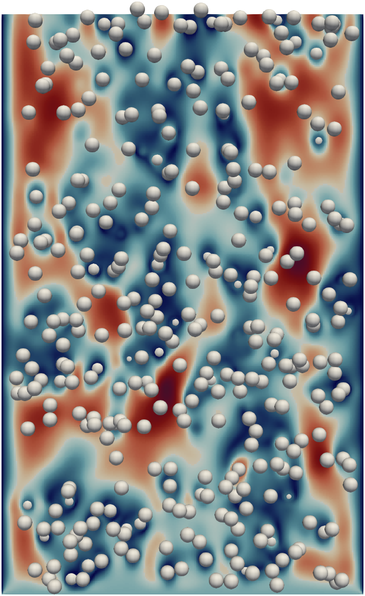
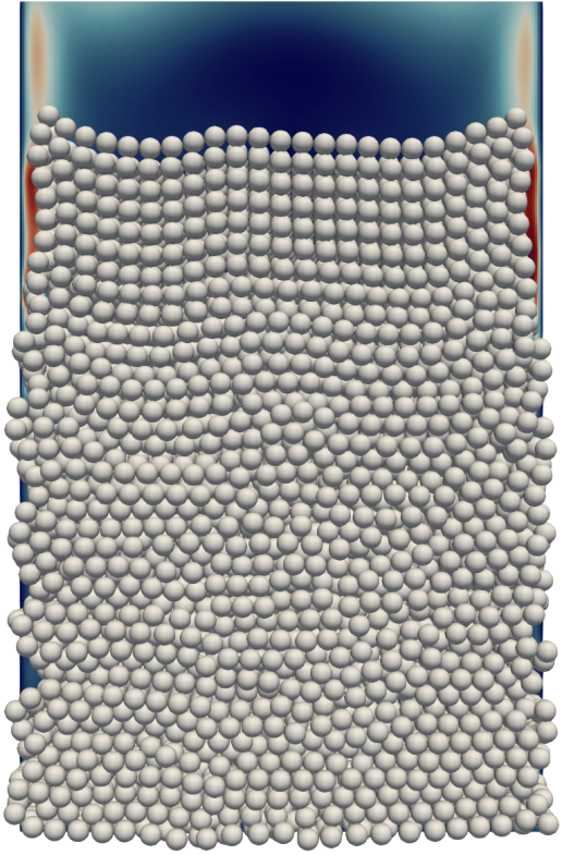
Figure 5: Visualization of the fluidized bed setup running on one CPU-GPU pair. Dilute case on the left, dense case on the right. For the fluid field, only a two-dimensional slice is visualized.

4.2 Performance results

In this section, we present and analyze the performance results. We first look into the scaling of the PD on multiple CPU cores to assess our initial assumption that the particle simulation part of such a coupled simulation would not benefit from a GPU parallelization. Next, we look at the individual run times of the different simulation components to understand the bottlenecks. Furthermore, we present a weak scaling benchmark for both cases up to 1024 CPU-GPU pairs. Finally, we demonstrate the acceleration potential of hybrid implementations by comparing it to a large-scale CPU-only simulation from the literature. For all results, we average over 500 time steps. In the following, we will refer to the performance criteria formulated in the introduction.

4.2.1 Particle scaling on the CPU

Using OpenMP with static scheduling, we parallelize the PD simulation on the CPU. Per-particle computations (e.g., adding gravitational forces) are parallelized among the particles, and particle-particle interactions are parallelized among the linked cells in one dimension. We use multiple cores of a single CPU and measure the run time of the PD simulation. The parallel efficiency $E_{n}$ is defined based on the serial run time $t_{\text{s}}$ and the run time using $n$ cores in parallel $t_{\text{p}}(n)$:

$$E_{n}=\frac{t_{s}}{t_{\text{p}}(n)\cdot n}.$$ (27)

For a perfectly linear scaling code, i.e., $t_{\text{p}}(n)=t_{s}/n$, the maximum achievable parallel efficiency $E_{\max}$ is 1 $\forall n$. For a non-scaling code, i.e., $t_{\text{p}}(n)=t_{\text{s}}\ \forall n$, the minimum achievable parallel efficiency $E_{\min}$ is $1/n$. Fig. 6 reports the parallel efficiency of the PD simulation for both cases for up to six cores, i.e., the size of a NUMA domain. We do not use more cores than available in a NUMA domain since the PD implementation is not NUMA-aware.

Figure 6: Parallel efficiency inside a NUMA domain for both cases. The perfect scaling (Best) and non-scaling (Worst) form the upper and lower bound.

We observe a similar pattern regarding the parallel efficiency in both the dilute and the dense case. Both show a decrease down to around 45% for six cores.
A parallel efficiency of about 45% when using a comparatively small number of six cores is a poor scaling result. We expect this performance for several reasons. First, the PD simulation consists of ten subsequent sub-cycles per time step, each containing several consecutive tasks (see Fig. 3). Each task consists of an OpenMP parallel loop with an implicit OpenMP barrier at the end, causing idle threads to wait for all threads to end the loop. Second, modifying the force and torque of a particle must be enclosed with an atomic region to avoid race conditions, which harms the parallel efficiency, but is a central task and thus required in several PD routines. Third, the workload (for the DEM and lubrication routine) per particle can differ significantly depending on the particle’s location inside the domain. The latter aspects hold for the dense and the dilute case, explaining the poor parallel efficiency in both cases. The poor parallel efficiency of the particle methodology supports our initial assumption that the particle simulation part would not benefit from a GPU parallelization in the context of geometrically resolved coupled simulations.

4.2.2 Run times of different simulation components

We investigate the run times of the different simulation components to analyze the penalty introduced by the hybrid implementation, i.e., the CPU-GPU communication, assess the GPU performance, and detect the overall bottlenecks. To evaluate the performance of the PSM kernel on the GPU, we build a roofline model [38] for an LBM kernel. As this kernel is memory bound, we determine the maximal possible performance for the given kernel and hardware when fully utilizing the memory bandwidth (i.e., the performance lightspeed estimation). The PSM kernel comprises the LBM kernel plus additional memory transfers depending on the number of overlapping particles. As this number differs from cell to cell, the PSM roofline model is not straightforward. Therefore, we use the LBM model, keeping in mind that this is a too-optimistic performance lightspeed estimation. Since we use the D3Q19 lattice model, we read and write 19 PDFs per cell and time step. This results in 19 reads and 19 writes (double-precision), i.e., 304 bytes to update one lattice cell [39]. The domain consists of $8e7$ fluid cells. This results in the following minimal run time according to the roofline model:

$$T_{\min}=\frac{304\ \text{B/cell}\cdot 8e7\ \text{cells/time step}}{1400\ \text{GB/s}}=17.4\ \text{ms/time step}.$$ (28)

We divide the total run time into the following components: the PSM kernel (PSM), the CPU-GPU communication (comm), the particle mapping (mapping), setting the particle velocities (setU), reducing the hydrodynamic forces $\boldsymbol{F}_{\text{p},i}^{\text{fp}}$ and torques $\boldsymbol{T}_{\text{p},i}^{\text{fp}}$ on the particles (redF), computing the PD and finally the remaining tasks (other), e.g., the LBM boundary handling. Fig. 7 reports the run times per time step for these components using a single CPU-GPU pair.

Figure 7: Individual run times of the different simulation components on a CPU-GPU pair.

In the dilute case, the PSM kernel needs about 42% more time per time step than the LBM lightspeed estimation, and the dense case 83% more time. The CPU-GPU communication is negligible for both cases. All components take longer in the dense case than in the dilute case. While in the dilute case, the PSM kernel accounts for the majority of the run time, the PD simulation needs more time than the PSM kernel in the dense case. Still, most of the run time is spent on GPU routines in the dense case.
The penalty introduced by the hybrid implementation is negligible because we only transfer a small amount of double-precision values per particle but no fluid cells. The penalty, therefore, shows that a hybrid parallelization with the presented technique is a viable approach, and the first criterion is met. The performance of the PSM kernel is close to utilizing the total memory bandwidth of the A100, especially considering that the roofline model does not consider the memory traffic due to the solid part of the PSM kernel. Therefore, the second criterion is met. There is a significant performance gain for the PSM kernel on the GPU compared to a CPU-only implementation since the PSM kernel is utilizing almost the entire memory bandwidth, which is typically way lower on CPU s. Even in the dense case, the GPU run time accounts for most of the total time because the fluid workload is much higher than the particle workload. Therefore, the third criterion is met.

4.2.3 Weak scaling

When increasing the simulation domain further to simulate physically relevant scenarios, using a single CPU-GPU pair is often insufficient. Instead, multiple pairs or even multiple nodes of a supercomputer have to be used. Therefore, a satisfactory weak scaling is inevitable. For weak scaling, the problem size is increased with an increasing number of CPU-GPU pairs, keeping the workload per CPU-GPU pair constant. When having a perfect weak scaling, the performance per CPU-GPU pair stays constant, independent of the number of CPU-GPU pairs used. Performance is work over time. In the context of LBM, MLUPs is a standard performance metric for weak scaling, meaning how many mega lattice cell updates the hardware performs per second. We use the total run time for computing the MLUPs, containing both the CPU (particles) and the GPU (fluid, coupling) time. We have conducted a few benchmarking runs and will use the best sample in the following weak-scaling plots. We start with a single CPU-GPU pair and a single domain block as described in Section 4.1. We then double the number of CPU-GPU pairs several times until we reach 1024. At the same time, we double the domain blocks/size alternately in each direction: $2\times 1\times 1$ blocks (two GPU s), $2\times 2\times 1$ blocks (four GPU s), $2\times 2\times 2$ (eight GPU s), etc. Fig. 8 reports the weak scaling for both cases. To the best of our knowledge, this is the most extensive weak scaling of a hybrid fluid-particle implementation presented in the literature.

Figure 8: Weak scaling performance for both cases up to 1024 CPU-GPU pairs.

We observe a roughly three times higher performance for the dilute case than for the dense case. Both cases show a parallel efficiency decrease particularly strong in the beginning. The parallel efficiency is 71% in the dilute case and 53% in the dense case when using 1024 CPU-GPU pairs, which corresponds to a domain size of $8000\times 1600\times 6400=8.192\times 10^{10}$ fluid cells. A similar scaling behavior has been observed in the literature both for other hybrid [11] and CPU-only fluid-particle implementations [1].
Interpreting the overall weak scaling behavior requires an in-depth analysis of the scaling of the different simulation components. When using a single CPU-GPU pair, the dominating routines are the PD, the PSM kernel, and the coupling (i.e., particle mapping, setting the particle velocities and reducing the hydrodynamic forces $\boldsymbol{F}_{\text{p},i}^{\text{fp}}$ and torques $\boldsymbol{T}_{\text{p},i}^{\text{fp}}$ on the particles). Additionally, we must now consider the communication (comm) overhead that arises from using multiple CPU-GPU pairs. On the one hand, this is the PD communication (CPU-CPU communication), on the other hand, the PSM communication (GPU-GPU communication). Fig. 9 and Fig. 10 show the weak scaling behavior of the dominating simulation components for both cases. The communication numbers cover the communications themselves, but also load imbalances between two communication.

Figure 9: Weak scaling performance of the dominating components for the dilute case up to 1024 CPU-GPU pairs.

Figure 10: Weak scaling performance of the dominating components for the dense case up to 1024 CPU-GPU pairs.

The different components show similar qualitative scaling behavior when comparing the two cases. The PSM kernel scales quite well in both cases. The corresponding GPU-GPU communication (PSM comm) is negligible. The PD run time increases initially and then shows saturation. The CPU-CPU communication (PD comm) increases drastically, overtaking the run time of the PSM kernel and the coupling in the dense case. The PD and the corresponding communication are more relevant for the overall scaling in the dense case than in the dilute case. The coupling scales similarly to the PD.
The PSM workload per GPU stays constant in the weak scaling explaining the nearly perfect scaling. Since we are hiding the PSM communication (see Section 3), we expect it to be negligible. We expect the PD and the coupling run time to increase initially because the number of neighboring blocks increases. More neighboring blocks lead to more ghost particles per block, resulting in a higher workload. This effect fades out when blocks have neighbors in all directions resulting in an almost linear scaling from this point on. This phenomenon has been reported in the literature [1]. The methodology requires ten particle sub-cycles per time step and three communications per sub-cycle for a physically accurate simulation. Additionally, the simulation requires two CPU-CPU communications per time step apart from the sub-cycles (see Fig. 3). We have 32 CPU-CPU communications per time step, which cannot be hidden behind other routines. It is the dominating factor for the decrease of the overall weak scaling performance in both cases. We assume this is due to these frequent synchronizations between the processes and the high pressure on the network. Reducing the collision history is part of PD comm, which includes swapping old and new contact information. Since this swap is also necessary without using multiple CPU-GPU pairs, PD comm is bigger zero even when using a single CPU-GPU pair. Overall, we observe a weak scaling performance that justifies using multiple supercomputer nodes. Therefore, the fourth criterion is met.

4.2.4 Potential speedup of hybrid implementations

We expect that the speedup of the hybrid implementation compared to a CPU-only code $S_{\text{hyb}}$ can be estimated as

$$S_{\text{hyb}}\approx\frac{1}{1+frac_{\text{acc}}\cdot(\frac{BW_{\text{CPU}}}{BW_{\text{GPU}}}-1)},$$ (29)

where $BW_{\text{CPU}}$ and $BW_{\text{GPU}}$ are the CPU and GPU memory bandwidths. $frac_{\text{acc}}$ is the CPU-only run time fraction of the component accelerated by the hybrid implementation. In our case, this is the PSM and the coupling. We assume $frac_{\text{acc}}$ is memory bound. We compare our hybrid performance results with one of the largest CPU-only simulations of polydisperse sediment beds [6]. The authors conducted the latter simulation on 320 Intel Xeon Platinum 8174 CPU s. In total, they computed $2.25\cdot 10^{15}$ lattice cell updates in 48 hours, which leads to a performance of around 41 MLUPs per CPU vs. 377 MLUPs per CPU-GPU pair in the dense case when using 1024 GPU s. The latter numbers result in a measured speedup of around 9.2. For the Intel Xeon Platinum 8174, we measured a memory bandwidth $BW_{\text{CPU}}$ of 70 GB/s. The estimated speedup based on Eq. 29 is around 10.3 (assuming $frac_{\text{acc}}=0.95$ and $BW_{\text{GPU}}=1400\ \text{GB/s}$) which is similar to the measured speedup. The latter computation is only a rough estimate since it ignores effects due to different CPU s, networks, physical setups, etc.

5 Conclusion

In this paper, we have introduced a hybrid coupled fluid-particle implementation with geometrically resolved particles. We use GPU s for the fluid dynamics, whereas the particle simulation runs on CPU s. We have addressed the issue that in multiphysics simulations, different methodologies can have distinctly different computational properties, implying that the best-suited hardware architecture may differ between the simulation components. The paper has examined the performance of this approach for two cases of a fluidized bed simulation that differ significantly in terms of the number of particles per volume. The particle methodology scales poorly, reaching a parallel efficiency of about 45% when using only six CPU cores. This scaling result supports our initial assumption that the particle simulation part of such a coupled simulation would not benefit from a GPU parallelization. The penalty introduced by the hybrid implementation (i.e., CPU-GPU communication) is negligible because we are transferring only a small amount of data per particle but no fluid cells. The performance of the fluid simulation is close to utilizing the whole memory bandwidth of the A100, implying that the GPU is the best choice for the fluid simulation. In both cases, the GPU routines take most of the run time. In a weak scaling benchmark, the hybrid fluid-particle implementation reaches a parallel efficiency of 71% in the dilute case and 53% in the dense case when using 1024 CPU-GPU pairs. The PD methodology requires 32 CPU-CPU communications per time step which is the driving force for the decrease of the overall parallel efficiency. Our results are limited insofar as different numbers of particle sub-cycles, fluid cells per diameter, etc., will result in different performance results. We have formulated four criteria that a hybrid implementation must meet to be suitable for the responsible use of heterogeneous supercomputers. The performance results have shown that our hybrid implementation fulfills all criteria making it suitable for large-scale simulations on heterogeneous supercomputers. In the future, we plan to investigate the particle communications in more detail regarding the bottleneck and optimization possibilities. We have shown the acceleration potential of hybrid implementations. Therefore, we plan to run coupled fluid-particle simulations of unprecedented sizes to better understand complex physical phenomena occurring in sea and river beds.

Declaration of competing interest

The authors declare that they have no known competing financial interests or personal relationships that could have appeared to influence the work reported in this paper.

Data availability

Data is available on Zenodo: 10.5281/zenodo.7752954.

Funding

The authors thank the Deutsche Forschungsgemeinschaft (DFG, German Research Foundation) for funding the project 433735254. The DFG had no direct involvement in this paper.

Author ORCIDs

S. Kemmler, https://orcid.org/0000-0002-9631-7349; C. Rettinger, https://orcid.org/0000-0002-0605-3731; H. Köstler, https://orcid.org/0000-0002-6992-2690;

Author contributions

S. Kemmler: Conceptualization, Methodology, Software, Validation, Formal analysis, Investigation, Data Curation, Writing - Original Draft, Visualization, Project administration; C. Rettinger: Conceptualization, Writing - Review and Editing; H. Köstler: Resources, Writing - Review and Editing, Supervision, Funding acquisition;

References

- [1] C. Rettinger, C. Godenschwager, S. Eibl, T. Preclik, T. Schruff, R. Frings, U. Rüde, Fully Resolved Simulations of Dune Formation in Riverbeds, in: J. M. Kunkel, R. Yokota, P. Balaji, D. Keyes (Eds.), High Performance Computing, Vol. 10266, Springer International Publishing, Cham, 2017, pp. 3–21. doi:10.1007/978-3-319-58667-0_1.
- [2] C. Schwarzmeier, C. Rettinger, S. Kemmler, J. Plewinski, F. Núñez-González, H. Köstler, U. Rüde, B. Vowinckel, Particle-resolved simulation of antidunes in free-surface flows (2023). arXiv:arXiv:2301.10674.
- [3] A. G. Kidanemariam, M. Uhlmann, Direct numerical simulation of pattern formation in subaqueous sediment, Journal of Fluid Mechanics 750 (2014) R2. doi:10.1017/jfm.2014.284.
- [4] Z. Benseghier, P. Cuéllar, L.-H. Luu, S. Bonelli, P. Philippe, A parallel GPU-based computational framework for the micromechanical analysis of geotechnical and erosion problems, Computers and Geotechnics 120 (2020) 103404. doi:10.1016/j.compgeo.2019.103404.
- [5] B. Vowinckel, T. Kempe, J. Fröhlich, Fluid–particle interaction in turbulent open channel flow with fully-resolved mobile beds, Advances in Water Resources 72 (2014) 32–44. doi:10.1016/j.advwatres.2014.04.019.
- [6] C. Rettinger, S. Eibl, U. Rüde, B. Vowinckel, Rheology of mobile sediment beds in laminar shear flow: Effects of creep and polydispersity, Journal of Fluid Mechanics 932 (2022) A1. doi:10.1017/jfm.2021.870.
- [7] T. Shimokawabe, T. Endo, N. Onodera, T. Aoki, A Stencil Framework to Realize Large-Scale Computations Beyond Device Memory Capacity on GPU Supercomputers, in: 2017 IEEE International Conference on Cluster Computing (CLUSTER), IEEE, Honolulu, HI, USA, 2017, pp. 525–529. doi:10.1109/CLUSTER.2017.97.
- [8] D. Rohr, S. Kalcher, M. Bach, A. A. Alaqeeliy, H. M. Alzaidy, D. Eschweiler, V. Lindenstruth, S. B. Alkhereyfy, A. Alharthiy, A. Almubaraky, I. Alqwaizy, R. Bin Suliman, An Energy-Efficient Multi-GPU Supercomputer, in: 2014 IEEE Intl Conf on High Performance Computing and Communications, 2014 IEEE 6th Intl Symp on Cyberspace Safety and Security, 2014 IEEE 11th Intl Conf on Embedded Software and Syst (HPCC,CSS,ICESS), IEEE, Paris, 2014, pp. 42–45. doi:10.1109/HPCC.2014.14.
- [9] G. Oyarzun, R. Borrell, A. Gorobets, A. Oliva, Portable implementation model for CFD simulations. Application to hybrid CPU/GPU supercomputers, International Journal of Computational Fluid Dynamics 31 (9) (2017) 396–411. doi:10.1080/10618562.2017.1390084.
- [10] M. Holzer, M. Bauer, H. Köstler, U. Rüde, Highly efficient lattice Boltzmann multiphase simulations of immiscible fluids at high-density ratios on CPUs and GPUs through code generation, The International Journal of High Performance Computing Applications 35 (4) (2021) 413–427. doi:10.1177/10943420211016525.
- [11] C. Kotsalos, J. Latt, J. Beny, B. Chopard, Digital blood in massively parallel CPU/GPU systems for the study of platelet transport, Interface Focus 11 (1) (2021) 20190116. doi:10.1098/rsfs.2019.0116.
- [12] Y. He, F. Muller, A. Hassanpour, A. E. Bayly, A CPU-GPU cross-platform coupled CFD-DEM approach for complex particle-fluid flows, Chemical Engineering Science 223 (2020) 115712. doi:10.1016/j.ces.2020.115712.
- [13] M. Sousani, A. M. Hobbs, A. Anderson, R. Wood, Accelerated heat transfer simulations using coupled DEM and CFD, Powder Technology 357 (2019) 367–376. doi:10.1016/j.powtec.2019.08.095.
- [14] D. Jajcevic, E. Siegmann, C. Radeke, J. G. Khinast, Large-scale CFD–DEM simulations of fluidized granular systems, Chemical Engineering Science 98 (2013) 298–310. doi:10.1016/j.ces.2013.05.014.
- [15] M. Xu, F. Chen, X. Liu, W. Ge, J. Li, Discrete particle simulation of gas–solid two-phase flows with multi-scale CPU–GPU hybrid computation, Chemical Engineering Journal 207–208 (2012) 746–757. doi:10.1016/j.cej.2012.07.049.
- [16] H. Norouzi, R. Zarghami, N. Mostoufi, New hybrid CPU-GPU solver for CFD-DEM simulation of fluidized beds, Powder Technology 316 (2017) 233–244. doi:10.1016/j.powtec.2016.11.061.
- [17] P. Valero-Lara, F. D. Igual, M. Prieto-Matías, A. Pinelli, J. Favier, Accelerating fluid–solid simulations (Lattice-Boltzmann & Immersed-Boundary) on heterogeneous architectures, Journal of Computational Science 10 (2015) 249–261. doi:10.1016/j.jocs.2015.07.002.
- [18] J. R. d. S. Junior, E. W. Clua, A. Montenegro, P. A. Pagliosa, Fluid Simulation with Two-Way Interaction Rigid Body Using a Heterogeneous GPU and CPU Environment, in: 2010 Brazilian Symposium on Games and Digital Entertainment, IEEE, Florianpolis, Santa Catarina, TBD, Brazil, 2010, pp. 156–164. doi:10.1109/SBGAMES.2010.25.
- [19] D. Roehm, A. Arnold, Lattice Boltzmann simulations on GPUs with ESPResSo, The European Physical Journal Special Topics 210 (1) (2012) 89–100. doi:10.1140/epjst/e2012-01639-6.
- [20] B. Sheikh, A. Pak, Numerical investigation of the effects of porosity and tortuosity on soil permeability using coupled three-dimensional discrete-element method and lattice Boltzmann method, Physical Review E 91 (5) (2015) 053301. doi:10.1103/PhysRevE.91.053301.
- [21] A. Khan, H. Sim, S. S. Vazhkudai, A. R. Butt, Y. Kim, An Analysis of System Balance and Architectural Trends Based on Top500 Supercomputers, in: The International Conference on High Performance Computing in Asia-Pacific Region, ACM, Virtual Event Republic of Korea, 2021, pp. 11–22. doi:10.1145/3432261.3432263.
- [22] J. Kim, S. Seo, J. Lee, J. Nah, G. Jo, J. Lee, SnuCL: An OpenCL framework for heterogeneous CPU/GPU clusters, in: Proceedings of the 26th ACM International Conference on Supercomputing, ACM, San Servolo Island, Venice Italy, 2012, pp. 341–352. doi:10.1145/2304576.2304623.
- [23] C. Rettinger, U. Rüde, A comparative study of fluid-particle coupling methods for fully resolved lattice Boltzmann simulations, Computers & Fluids 154 (2017) 74–89. doi:10.1016/j.compfluid.2017.05.033.
- [24] C. Rettinger, U. Rüde, An efficient four-way coupled lattice Boltzmann – discrete element method for fully resolved simulations of particle-laden flows, Journal of Computational Physics 453 (2022) 110942. doi:10.1016/j.jcp.2022.110942.
- [25] T. Krüger, H. Kusumaatmaja, A. Kuzmin, O. Shardt, G. Silva, E. M. Viggen, The Lattice Boltzmann Method: Principles and Practice, Graduate Texts in Physics, Springer International Publishing, Cham, 2017. doi:10.1007/978-3-319-44649-3.
- [26] Y. H. Qian, D. D’Humières, P. Lallemand, Lattice BGK Models for Navier-Stokes Equation, Europhysics Letters (EPL) 17 (6) (1992) 479–484. doi:10.1209/0295-5075/17/6/001.
- [27] X. He, L.-S. Luo, Lattice Boltzmann Model for the Incompressible Navier–Stokes Equation, Journal of Statistical Physics 88 (3/4) (1997) 927–944. doi:10.1023/B:JOSS.0000015179.12689.e4.
- [28] A. J. C. Ladd, R. Verberg, Lattice-Boltzmann Simulations of Particle-Fluid Suspensions, Journal of Statistical Physics 104 (5) (2001) 1191–1251. doi:10.1023/A:1010414013942.
- [29] P. A. Cundall, O. D. L. Strack, A discrete numerical model for granular assemblies, Géotechnique (1979). doi:10.1680/geot.1979.29.1.47.
- [30] Y. Fukumoto, H. Yang, T. Hosoyamada, S. Ohtsuka, 2-D coupled fluid-particle numerical analysis of seepage failure of saturated granular soils around an embedded sheet pile with no macroscopic assumptions, Computers and Geotechnics 136 (2021) 104234. doi:10.1016/j.compgeo.2021.104234.
- [31] B. D. Jones, J. R. Williams, Fast computation of accurate sphere-cube intersection volume, Engineering Computations 34 (4) (2017) 1204–1216. doi:10.1108/EC-02-2016-0052.
- [32] M. Bauer, S. Eibl, C. Godenschwager, N. Kohl, M. Kuron, C. Rettinger, F. Schornbaum, C. Schwarzmeier, D. Thönnes, H. Köstler, U. Rüde, waLBerla: A block-structured high-performance framework for multiphysics simulations, Computers & Mathematics with Applications 81 (2021) 478–501. doi:10.1016/j.camwa.2020.01.007.
- [33] S. Eibl, U. Rüde, A Modular and Extensible Software Architecture for Particle Dynamics (2019). arXiv:arXiv:1906.10963.
- [34] M. Bauer, H. Köstler, U. Rüde, Lbmpy: Automatic code generation for efficient parallel lattice Boltzmann methods, Journal of Computational Science 49 (2021) 101269. doi:10.1016/j.jocs.2020.101269.
- [35] D. Ernst, M. Holzer, G. Hager, M. Knorr, G. Wellein, Analytical performance estimation during code generation on modern GPUs, Journal of Parallel and Distributed Computing 173 (2023) 152–167. doi:10.1016/j.jpdc.2022.11.003.
- [36] E. Biegert, B. Vowinckel, E. Meiburg, A collision model for grain-resolving simulations of flows over dense, mobile, polydisperse granular sediment beds, Journal of Computational Physics 340 (2017) 105–127. doi:10.1016/j.jcp.2017.03.035.
- [37] P. Costa, B. J. Boersma, J. Westerweel, W.-P. Breugem, Collision model for fully resolved simulations of flows laden with finite-size particles, Physical Review E 92 (5) (2015) 053012. doi:10.1103/PhysRevE.92.053012.
- [38] G. Hager, G. Wellein, Introduction to High Performance Computing for Scientists and Engineers, zeroth Edition, CRC Press, 2010. doi:10.1201/EBK1439811924.
- [39] C. Feichtinger, J. Habich, H. Köstler, U. Rüde, T. Aoki, Performance modeling and analysis of heterogeneous lattice Boltzmann simulations on CPU–GPU clusters, Parallel Computing 46 (2015) 1–13. doi:10.1016/j.parco.2014.12.003.