Kondo enhancement of current induced spin accumulation in a quantum dot

Abstract

Weak spin-orbit coupling produces very limited current induced spin accumulation in semiconductor nanostructures. We demonstrate a possibility to increase parametrically the spin polarization using the Kondo effect. As a model object we consider a quantum dot side coupled to a quantum wire taking into account the spin dependent electron tunneling from the wire to the dot. Using the nonequilibrium Green’s functions, we show that the many body correlations between the quantum dot and the quantum wire can increase the current induced spin accumulation at low temperatures by almost two orders of magnitude for the moderate system parameters. The enhancement is related to the Kondo peak formation in the density of states and the spin instability due to the strong Coulomb interaction. This effect may be useful to electrically manipulate the localized electron spins in quantum dots for their quantum applications.

I Introduction

Semiconductor quantum dots (QDs) hold a great promise for the scalable quantum information processing using the localized spins in QDs as qubits [1, 2, 3, 4, 5]. The electron and hole spins can be efficiently oriented [6, 7, 8], manipulated [9, 10, 11, 12] and read out [13, 14, 15] by optical means. However, electrical schemes being based on the highly advanced fabrication technology suggest larger ensembles of individually addressable qubits. On this way, the electrical spin transport, spin correlations, and spin read out are already firmly established [16, 17, 18, 19, 20, 21]. Only the electrical single spin polarization without magnetic field remains elusive for years.

This stumbling block on the way of quantum technologies can be removed by the current induced spin polarization effect [22]. The nonequilibrium flow of charge carriers breaks the time inversion symmetry and allows for the polarization of electron spins in the system. This effect was first predicted [23] and observed [24] in bulk Te crystals. Later it was extended to the epilayers [25] and quantum wells [26, 27] based on GaAs-like semiconductors. Nowadays the related effect of chirality induced spin selectivity is in the focus of intense theoretical and experimental investigations [28, 29, 30].

Generally, the degree of current induced spin polarization is small. This is related to the weakness of the spin-orbit coupling and the small ratio of the drift and Fermi velocities [31]. A number of approaches to overcome these factors were suggested such as: spin-momentum locking [32, 33, 34], streaming conductivity regime [35, 36], hopping conductivity [37, 38], and exploitation of the valence band spin-orbit splitting [39, 40]. In this Letter, we demonstrate that the spin polarization can be drastically increased at low temperatures due to the Kondo many body correlations. Notably, this Kondo enhancement of the spin accumulation can be combined with the previously established tools to obtain the largest spin polarization.

As a model system, we consider a QD side coupled to a quantum wire, see Fig. 1. The structure is assumed to be gate defined in two dimensional electron or hole gas. The spin-orbit interaction gives rise to the spin dependent tunneling. It leads to the spin accumulation in the QD under current flow in the quantum wire [40], similar to the spin Hall [41] and Mott [42] effects. At the same time, the Coulomb interaction in the QD produces the many body correlations and leads to the Kondo effect [43]. This effect is known to enhance conductivity and the spin susceptibility to external magnetic field [44]. Here, we demonstrate also the enhancement of the current induced spin accumulation effect.

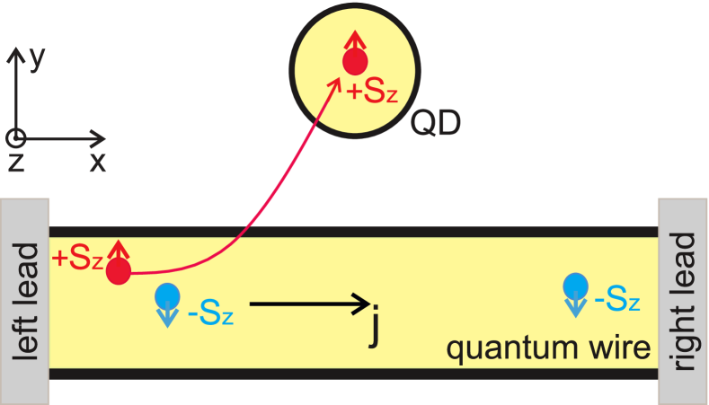
Figure 1: Sketch of a QD side coupled to a quantum wire. The difference of the tunneling probabilities for spin up (red balls with arrows) and spin down (blue ones) particles leads to the current induced spin accumulation in the QD.

II Model

The $C_{2v}$ point symmetry group of the system allows for the linear coupling between the $x$ component of a vector and the $z$ component of a pseudovector, i.e. between the electric current along the wire and the spin polarization in the QD along the growth axis, see Fig. 1. To describe this coupling microscopically, we adopt the Anderson Hamiltonian [45]:

$$\mathcal{H}=E_{0}\sum_{\pm}n_{\pm}+Un_{+}n_{-}+\sum_{k,\pm}E_{k}n_{k,\pm}\\ +\sum_{k,\pm}\left(V_{k,\pm}d_{\pm}^{\dagger}c_{k,\pm}+{\rm H.c.}\right).$$ (1)

Here $E_{0}$ is a single particle energy in the QD, $n_{\pm}=d_{\pm}^{\dagger}d_{\pm}$ are the occupancies of the corresponding spin up and spin down states expressed through the annihilation operators $d_{\pm}$, $U$ is the Coulomb repulsion energy, $E_{k}$ describes the dispersion of particles in the quantum wire with the wave vector $k$ along the wire, and $n_{k,\pm}=c_{k,\pm}^{\dagger}c_{k,\pm}$ are the occupancies of the corresponding spin states expressed through the annihilation operators $c_{k,\pm}$. We assume the wire to be ballistic and also neglect the interactions in it. Finally, the coefficients $V_{k,\pm}$ describe the spin dependent tunneling between the quantum wire and the QD. Note, that the spin dependence in the form $V_{k,+}\neq V_{k,-}$ is allowed for any crystal structure of the host semiconductors, so the current induced spin accumulation is equally possible for GaAs, Si, and Ge-based heterostructures. The time reversal symmetry imposes a relation $V_{k,+}=V_{-k,-}^{*}$.

The spin-orbit coupling can lead to the spin splitting of the electron dispersion in the quantum wire. This however requires low symmetry of the system compared to the spin dependent tunneling and is not important for the current induced spin accumulation in the QD separated from the quantum wire by a tunnel barrier. The ratio of $V_{k,+}$ and $V_{k,-}$ determines the chirality of the quasi bound state in the QD [46, 47, 48, 49]. For completely chiral quasi bound state $V_{k_{0},-}=V_{-k_{0},+}=0$ and $\left|V_{k_{0},+}\right|=\left|V_{-k_{0},-}\right|\neq 0$, so the spin orientation in the QD is locked to the propagation direction along the quantum wire (here $k_{0}>0$ is determined by the relation $E_{k_{0}}=E_{0}$). We have shown recently, that this limit can be reached in the heterostructures with the two dimensional hole gas due to the complex valence band structure [40]. In what follows, we focus mainly on the completely chiral states and discuss the case of finite chirality in the end of the Letter.

III Formalism

For the calculation of the current induced spin accumulation in the QD as a function of the bias applied to the quantum wire, we use the nonequilibrium Green’s functions [50, 51, 52]. This approach despite having disadvantages [53], allows us to account for the Kondo effect even beyond the linear response regime in the simplest way and to demonstrate the Kondo enhancement of current induced spin accumulation. The truncation of the system of the Heisenberg equations of motion allows one to obtain a closed set of equations for the operators $d_{\pm}$, $c_{k,\pm}$, $d_{\pm}n_{\mp}$, $c_{k,\pm}n_{\mp}$, $c_{k,\mp}^{\dagger}d_{\mp}d_{\pm}$, and $c_{k,\mp}d_{\mp}^{\dagger}d_{\pm}$. From its solution one finds the retarded Green’s functions of spin up and spin down particles in the QD $G_{\pm}^{R}(\omega)$. In particular, in the limit of the large Coulomb repulsion, $U\to\infty$, one obtains ($\hbar=1$) [54, 55, 56]

$$G_{\pm}^{R}(\omega)=\frac{1-\left\langle n_{\mp}\right\rangle}{\omega-E_{0}-\Sigma_{0}(\omega)-\Sigma_{1,\pm}(\omega)},$$ (2)

where $\left\langle n_{\mp}\right\rangle$ are the average occupancies of the QD states, which should be determined self consistently. The self energies $\Sigma_{0}(\omega)$ and $\Sigma_{1,\pm}(\omega)$ in the wide band approximation have the form

$$\Sigma_{0}(\omega)=\frac{\Gamma}{\pi}\int\limits_{-W}^{W}\frac{1}{\omega-E+{\rm i}0}\mathrm{d}E,$$ (3a)

$$\Sigma_{1,\pm}(\omega)=\frac{\Gamma}{\pi}\int\limits_{-W}^{W}\frac{f_{R/L}(E)}{\omega-E+{\rm i}0}\mathrm{d}E.$$ (3b)

Here $\Gamma$ is the tunneling rate between the QD and the quantum wire, $W$ is the band width, and

$$f_{L/R}(E)=\frac{1}{1+\exp\left[(E-E_{F}^{L/R})/T\right]}$$ (4)

are the Fermi distribution functions in the left and right leads with $T$ being the temperature ($k_{B}=1$), and $E_{F}^{L/R}$ being the Fermi energies in the left/right leads. Eq. (2) is qualitatively correct in the weak coupling regime, when the temperature exceeds the Kondo temperature $T_{K}=W\exp\left(-\pi|E_{F}-E_{0}|/\Gamma\right)$.

The density of states related to the QD is given by $D(\omega)=-\mathop{\rm Im}\left[G_{+}^{R}(\omega)+G_{-}^{R}(\omega)\right]/\pi$. It is shown in Fig. 2(a) for the thermal equilibrium, $E_{F}^{L}=E_{F}^{R}$, and different temperatures. Generally it consists of a broad peak with the width $\sim\Gamma$ at the QD energy $E_{0}$ (which is a bit renormalized due to the tunneling) and a narrow peak at the Fermi energy, which leads to the Kondo effect. The peak has a width of the order of $T_{K}$ and disappears with increase of the temperature, as one can see in Fig. 2(a).

To calculate the occupancies of the spin states in the QD, we consider the expressions for the current to the QD from the left/right lead corresponding to spin up/down particles [57]:

$$J_{L/R}=e\Gamma\int\frac{\mathrm{d}\omega}{2\pi}\left[{\rm i}G_{+/-}^{<}(\omega)-2f_{L/R}(\omega)\mathop{\rm Im}G_{+/-}^{R}(\omega)\right],$$ (5)

where $G_{\pm}^{<}(\omega)$ are the lesser Green’s functions of the QD. In the steady state, these currents vanish, which yields the desired occupancies:

$$\left\langle n_{+/-}\right\rangle=-{\rm i}\int\frac{\mathrm{d}\omega}{2\pi}G_{+/-}^{<}(\omega)\\ =-\int\limits_{-W}^{W}\frac{\mathrm{d}\omega}{\pi}f_{L/R}(\omega)\mathop{\rm Im}G_{+/-}^{R}(\omega).$$ (6)

Here the retarded Green’s functions also depend on the occupancies, Eq. (2), so they should be calculated self consistently. Ultimately, the spin polarization in the QD is given by

$$P=\frac{\left\langle n_{+}\right\rangle-\left\langle n_{-}\right\rangle}{\left\langle n_{+}\right\rangle+\left\langle n_{-}\right\rangle}.$$ (7)

Its calculation and analysis is the main goal of this work.

IV Results

The spin polarization induced by the electric current is shown in Fig. 2(b) as a function of the bias $eV$, which is applied symmetrically: $E_{F}^{L/R}=E_{F}\pm eV/2$. This dependence looks the same for the three temperatures $T=T_{K}$, $20T_{K}$ and $0.1\Gamma$ shown in the figure. Qualitatively, the bias produces the difference of the fluxes of the particles moving to the left and to the right along the quantum wire, and since the tunneling matrix elements depend on the spin and direction of the propagation, this results in the current induced spin accumulation in the QD. At the same time, the large bias $eV\sim\Gamma\gg T_{K}$ destroys many body correlations, so the dependences shown in Fig. 2(b) overlap for the different temperatures. The spin polarization is an odd function of the bias in agreement with the time reversal symmetry. It increases with increase of the bias and saturates at $|eV|>2|E_{F}-E_{0}|$. The polarization approaches 100% when the quasi bound state in the QD with the width $\Gamma$ lies completely below the Fermi energy in one lead and above the Fermi energy in the other lead.

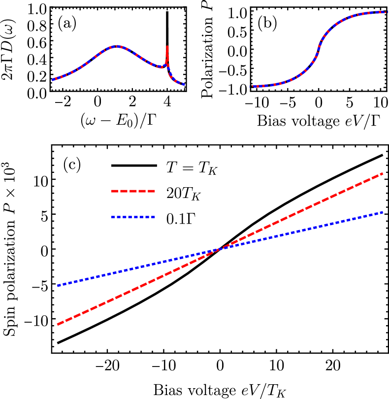
Figure 2: (a) Density of states related to the QD calculated after Eq. (2). (b) Degree of spin polarization in the QD [Eq. (7)] as a function of the applied bias. (c) The same as in (b) for smaller voltages. The solid black, red dashed and blue dotted curves for all panels are calculated for the different temperatures given in the legend in (c). The other parameters are $E_{F}-E_{0}=4\Gamma$ and $W=100\Gamma$.

The many body correlations, which lead to the Kondo effect, manifest themselves at the smallest voltages, $eV\sim T_{K}$, as shown in Fig. 2(c). Here the same curves as in Fig. 2(b) are zoomed in. One can see, that the current induced spin accumulation is in fact temperature dependent for the smallest voltages: the higher the temperature, the smaller the polarization. For the large voltages the curves for the low temperatures approach the curve for the high temperature.

This suggests the introduction of the spin susceptibility $\chi_{s}$ for the current induced spin accumulation as

$$\chi_{s}=\lim_{V\to 0}\frac{P}{eV}.$$ (8)

Its temperature dependence is shown in Fig. 3(a) by the black curve for the same parameters as in Fig. 2. One can see that it strongly increases with decrease of temperature. Note that our approach is valid as long as $T>T_{K}$ only, and $T_{K}=3.5\cdot 10^{-4}\,\Gamma$ for these parameters.

Figure 3: (a) The spin susceptibility as a function of temperature calculated numerically (black solid curve), analytically (gray dotted curve), and in the Hartree–Fock approximation (red dashed curve) for the same parameters as in Fig. 2. (b) The ratio of the spin susceptibilities calculated with and without many body correlations, $\chi_{s}/\chi_{s}^{(0)}$, as a function of the scaled temperature $\Theta$ [Eq. (10)] for the same parameters as in Fig. 2 except for the larger ratios of the Fermi energy and the band width $(E_{F}-E_{0})/W=0.13$ and $0.4$ for the red dashed and blue dotted curves, respectively.

The gray dashed curve represents an analytical approximation, which is quite cumbersome and is given in the Supplemental Material [58]. Its analysis for low temperatures $T\gtrsim T_{K}$ shows that the spin susceptibility can be estimated as

$$\chi_{s}\sim\frac{1}{\Gamma}\times\frac{E_{F}-E_{0}}{\Gamma}.$$ (9)

Here the first factor reflects the fact that the density of states has a maximum at the Fermi energy of the order of $1/\Gamma$ caused by the many body correlations (Kondo peak), so the difference of the occupancies in the leads sharply affects the occupancies of the spin states in the QD. The second factor is related to the interaction induced instability: once the spin up electron enters the QD, it suppresses the tunneling of the spin down electron, so the spin polarization increases.

For comparison, the red dashed curve in Fig. 3(a) shows the spin susceptibility $\chi_{s}^{(0)}$ calculated neglecting the many body correlations (Hartree-Fock approximation) [58]. At high temperatures $T\gtrsim\Gamma$ it coincides with the black curve. However, at low temperatures, $T\ll\Gamma$, this approximation strongly underestimates the spin susceptibility and gives $\chi_{s}\sim 1/(E_{F}-E_{0})$.

To underline the role of many body correlations in the effect of current induced spin accumulation, we plot the ratio $\chi_{s}/\chi_{s}^{(0)}$ in Fig. 3(b) as a function of scaled temperature

$$\Theta=\frac{\ln(T/T_{K})}{\ln(\Gamma/T_{K})}.$$ (10)

This parameter equals zero when $T=T_{K}$, equals unity when $T=\Gamma$ and logarithmically scales in between (note that our approach is valid for $\Theta>0$ only). The black curve in Fig. 3(b) is calculated for the same parameters as Fig. 3 and shows that the ratio $\chi_{s}/\chi_{s}^{(0)}$ exceeds 10 when temperature approaches the Kondo temperature. The red dashed and blue dotted curves are calculated for the chiral quasi bound state located deeper below the Fermi energy, i.e. larger $(E_{F}-E_{0})/W$. For simplicity of the numerical calculations, we tuned this dimensionless parameter by decreasing the band width $W$. One can see that the deeper the localization (or the larger the Fermi energy, or the smaller the band width) the larger role of the many body correlations. In particular, the increase of the spin susceptibility due to them approaches 100 at low temperatures, as shown by the blue dotted curve. This is the main result of this work.

V Discussion

Above we considered a completely chiral quasi bound state (i.e. $V_{-|k|,+}=V_{|k|,-}=0$). Generally, for arbitrary bias the results do not change qualitatively for the weaker chirality, but the current induced spin accumulation decreases. In particular case of small bias, the spin susceptibility is simply proportional to the chirality, $\chi_{s}\propto\mathcal{C}=\left(|V_{k_{0},+}^{2}|-|V_{k_{0},-}^{2}|\right)/\left(|V_{k_{0},+}^{2}|+|V_{k_{0},-}^{2}|\right)$ [58].

As an outlook, we believe that the predicted enhancement of the current induced spin accumulation by the many body correlations is a general phenomenon. So it would be important to apply other theoretical approaches such as the numerical renormalization group method [59, 60, 61], to establish scaling relations in the strong coupling regime at temperatures below $T_{K}$, and to study the manifestations of the current induced spin accumulation in the transport properties. Qualitatively, we note that the completely chiral quasi bound state does not lead to the back scattering of the particles in the quantum wire, because each spin state is coupled to the particles propagating only in one direction. Thus the increase of chirality $C$ leads to the disappearance of the Kondo resonance in the differential conductivity. In addition, the current induced spin accumulation in the QD can be probed optically by means of the polarized photoluminescence and spin induced Faraday rotation of the probe light, or electrically using point contacts [62, 63] and scanning tunneling microscopy [64]. We note that the Onsager relations also imply that the spin pumping of the QD by external means would lead to the electric current along the quantum wire.

The proposed model allows for various generalizations, which can be studied theoretically and experimentally. For example, it would be interesting to take into account interactions between the particles in the quantum wire or consider a few QDs side coupled to the quantum wire. The spin accumulation in the QD can be also induced by the different temperatures in the leads similar to the spin Nernst effect.

The typical parameters of the system for the experimental realization of the current induced spin accumulation are the lengths of the order of $100$ nm and the coupling strength $\Gamma\sim 10~{}\mu$eV. Then, for example, for the parameters used in Fig. 2 we obtain $T_{K}\sim 50~{}\mu$K, which is quite low. We note however, that the many body correlations significantly enhance the spin polarization even at the temperatures smaller than, but comparable to $\Gamma\sim 100$ mK, which is easier to reach.

Indeed, a very similar system was recently realized experimentally [65]. However, the QD was placed inside the quantum wire, so the quasi bound state was not chiral and the effect of the current induced spin accumulation was symmetry forbidden. If QD is shifted along $y$ direction, our theory predicts significant spin polarization increased by the Kondo effect in this system.

VI Conclusion

We have demonstrated that the Kondo effect can be exploited to enhance the spin galvanic effects such as the current induced spin accumulation. In particular, the many body correlations are shown to parametrically increase the degree of the spin polarization in chiral quasi bound state in the QD side coupled to the quantum wire. The spin susceptibility to the electric current can be enhanced by almost two orders of magnitude for the realistic system parameters.

We thank I. V. Krainov for fruitful discussions and the Foundation for the Advancement of Theoretical Physics and Mathematics “BASIS”. Analytical calculations by D.S.S. were supported by the Russian Science Foundation grant No. 21-72-10035. V.N.M. acknowledges support from the Interdisciplinary Scientific and Educational School of Moscow University “Photonic and Quantum technologies. Digital medicine”.

Supplemental Material includes the following topics:

toc

S1 S1. Derivation of Green’s functions

Here we present for the completeness the derivation of the retarded Green’s functions for the Anderson Hamiltonian. We follow the approach of Ref. 1, which is explained in more detail in Ref. 2.

We start from the Hamiltonian [Eq. (1) in the main text]

$$\mathcal{H}=E_{0}\sum_{\pm}n_{\pm}+Un_{+}n_{-}+\sum_{k,\pm}E_{k}n_{k,\pm}\\ +\sum_{k,\pm}\left(V_{k,\pm}d_{\pm}^{\dagger}c_{k,\pm}+{\rm H.c.}\right),$$ (S1)

where $E_{0}$ is the localization energy in the QD, $n_{\pm}=d_{\pm}^{\dagger}d_{\pm}$ are the occupancies of the spin up and spin down states in the quantum dot (QD) with $d_{\pm}$ ($d_{\pm}^{\dagger}$) being the corresponding annihilation (creation) operators, $U$ is the Coulomb repulsion energy in the QD, $E_{k}$ is the spin independent dispersion of the states in the quantum wire with $k$ being the wave vector along the wire, $n_{k,\pm}=c_{k,\pm}^{\dagger}c_{k,\pm}$ are the occupancies of the spin up and spin down states with the wave vector $k$ in the wire with $c_{k,\pm}$ ($c_{k,\pm}^{\dagger}$) being the corresponding annihilation (creation) operators, and finally $V_{k,\pm}$ are the spin dependent tunneling matrix elements between the quantum wire and the QD. The time inversion symmetry implies that

$$V_{k,+}=V_{-k,-}^{*}.$$ (S2)

We note that for the previously investigated case of the hole in the complex valence band [3], the subscript $\pm$ for the states in the wire refers to the heavy holes with the spin $\pm 3/2$ along the structure growth axis (perpendicular to the plain containing the quantum wire and the QD), and it refers to the light holes with the spin $\mp 1/2$ in the QD along the same axis.

The retarded Green’s functions can be obtained from the following Heisenberg equations for the operators (${\hbar=1}$):

$${\rm i}\frac{\mathrm{d}d_{\pm}}{\mathrm{d}t}=E_{0}d_{\pm}+Ud_{\pm}n_{\mp}+\sum_{k}V_{k,\pm}^{*}c_{k,\pm},$$ (S3a)

$${\rm i}\frac{\mathrm{d}c_{k,\pm}}{\mathrm{d}t}=E_{k}c_{k,\pm}+V_{k,\pm}d_{\pm}$$ (S3b)

$${\rm i}\frac{\mathrm{d}(d_{\pm}n_{\mp})}{\mathrm{d}t}=(E_{0}+U)d_{\pm}n_{\mp}+\sum_{k}\left(V_{k,\pm}^{*}c_{k,\pm}n_{\mp}\right.\\ \left.+V_{k,\mp}c_{k,\mp}^{\dagger}d_{\pm}d_{\mp}-V_{k,\mp}^{*}c_{k,\mp}d_{\mp}^{\dagger}d_{\pm}\right),$$ (S3c)

$${\rm i}\frac{\mathrm{d}(c_{k,\pm}n_{\mp})}{\mathrm{d}t}=E_{k}c_{k,\pm}n_{\mp}+V_{k,\pm}d_{\pm}n_{\mp}\\ +\sum_{q}\left(-V_{q,\mp}c_{k,\pm}c_{q,\mp}^{\dagger}d_{\mp}+V_{q,\mp}^{*}c_{k,\pm}d_{\mp}^{\dagger}c_{q,\mp}\right),$$ (S3d)

$${\rm i}\frac{\mathrm{d}(c_{k,\mp}^{\dagger}d_{\pm}d_{\mp})}{\mathrm{d}t}=(2E_{0}+U-E_{k})c_{k,\mp}^{\dagger}d_{\pm}d_{\mp}+V_{k,\mp}^{*}d_{\pm}n_{\mp}\\ +\sum_{q}\left(V_{q,\pm}^{*}c_{k,\mp}^{\dagger}c_{q,\pm}d_{\mp}+V_{q,\mp}^{*}c_{k,\mp}^{\dagger}d_{\pm}c_{q,\mp}\right),$$ (S3e)

$${\rm i}\frac{\mathrm{d}(c_{k,\mp}d_{\mp}^{\dagger}d_{\pm})}{\mathrm{d}t}=E_{k}c_{k,\mp}d_{\mp}^{\dagger}d_{\pm}+V_{k,\mp}\left(d_{\pm}-d_{\pm}n_{\mp}\right)\\ +\sum_{q}\left(-V_{q,\mp}c_{k,\mp}c_{q,\mp}^{\dagger}d_{\pm}+V_{q,\pm}^{*}c_{k,\mp}d_{\mp}^{\dagger}c_{q,\pm}\right).$$ (S3f)

These equations allow one to calculate in the steady state the correlation functions of the operators $A$ and $B$ like

$$\left\langle A,B\right\rangle^{R}(t)\equiv-{\rm i}\left\langle A(t)B+BA(t)\right\rangle\theta(t)$$ (S4)

with $\theta(t)$ being the Heaviside step function from the equations

$$\frac{\mathrm{d}}{\mathrm{d}t}\left\langle A,B\right\rangle^{R}(t)=-{\rm i}\left\langle AB+BA\right\rangle\delta(t)+\left\langle\frac{\mathrm{d}A}{\mathrm{d}t},B\right\rangle^{R}(t),$$ (S5)

where $\delta(t)$ is the Dirac delta function.

Our aim is to calculate the retarded spin dependent Green’s functions

$$G_{\pm}^{R}(t)\equiv\left\langle d_{\pm},d_{\pm}^{\dagger}\right\rangle^{R}.$$ (S6)

Thus we consider $B=d_{\pm}^{\dagger}$ in Eq. (S5) and different operators $A$ from Eqs. (S3).

In the Hartree–Fock approximation one uses Eqs. (S3a—S3c), truncates the system using the approximations

$$c_{k,\pm}n_{\mp}=c_{k,\pm}\left\langle n_{\mp}\right\rangle,\qquad c_{k,\mp}^{\dagger}d_{\pm}d_{\mp}=c_{k,\mp}d_{\mp}^{\dagger}d_{\pm}=0,$$ (S7)

and uses the following correlators

$$\left\langle d_{\pm}^{\dagger}d_{\pm}+d_{\pm}d_{\pm}^{\dagger}\right\rangle=1,\qquad\left\langle d_{\pm}^{\dagger}c_{k,\pm}+c_{k,\pm}d_{\pm}^{\dagger}\right\rangle=0,\\ \left\langle d_{\pm}^{\dagger}d_{\pm}n_{\mp}+d_{\pm}n_{\mp}d_{\pm}^{\dagger}\right\rangle=\left\langle n_{\mp}\right\rangle,$$ (S8)

where $\left\langle n_{\pm}\right\rangle$ are the steady state occupancies of the spins states of the QD, which should be calculated self consistently. In this way, we obtain the Green’s functions in the limit of strong Coulomb interaction ($U\to\infty$) [2]

$$G_{\pm}^{R(0)}=\frac{1-\left\langle n_{\mp}\right\rangle}{\omega-E_{0}-\Sigma_{0}^{R}(1-\left\langle n_{\mp}\right\rangle)},$$ (S9)

where the self energy

$$\Sigma_{0}^{R}=\sum_{k}\frac{|V_{k,\pm}^{2}|}{\omega-E_{k}+{\rm i}0}$$ (S10)

is spin independent due to Eq. (S2).

The Hartree–Fock approximation does not capture the Kondo effect, therefore, it is necessary to go beyond Eq. (S7) and consider additional Eqs. (S3d—S3f). To truncate the system one uses the approximations

$$c_{k,\mp}^{\dagger}d_{\pm}c_{q,\mp}=-\delta_{k,q}f_{k}d_{\pm},\quad c_{k,\mp}c_{q,\mp}^{\dagger}d_{\pm}=\delta_{k,q}(1-f_{k})d_{\pm},\\ c_{k,\pm}c_{q,\mp}^{\dagger}d_{\mp}=c_{k,\pm}d_{\mp}^{\dagger}c_{q,\mp}=c_{k,\mp}^{\dagger}c_{q,\pm}d_{\mp}=c_{k,\mp}d_{\mp}^{\dagger}c_{q,\pm}=0,$$ (S11)

where ($k_{B}=1$)

$$f_{|k|}=\frac{1}{1+\exp\left[(E_{k}-E_{F}^{L})/T\right]}$$ (S12a)

and

$$f_{-|k|}=\frac{1}{1+\exp\left[(E_{k}-E_{F}^{R})/T\right]}$$ (S12b)

are the spin independent occupancies of the states with the wave vector $|k|$ ($-|k|$) in the quantum wire with $E_{F}^{L}$ ($E_{F}^{R}$) being the Fermi level in the left (right) lead. One also uses the following additional approximations for the correlation functions:

$$\left\langle d_{\pm}^{\dagger}c_{k,\mp}^{\dagger}d_{\pm}d_{\mp}+c_{k,\mp}^{\dagger}d_{\pm}d_{\mp}d_{\pm}^{\dagger}\right\rangle\\ =\left\langle d_{\pm}^{\dagger}c_{k,\mp}d_{\mp}^{\dagger}d_{\pm}+c_{k,\mp}d_{\mp}^{\dagger}d_{\pm}d_{\pm}^{\dagger}\right\rangle=0.$$ (S13)

In this way, we obtain the Green’s functions in the limit of large $U$ [1]:

$$G_{\pm}^{R}=\frac{1-\left\langle n_{\mp}\right\rangle}{\omega-E_{0}-\Sigma_{0}^{R}-\Sigma_{1,\pm}^{R}},$$ (S14)

where

$$\Sigma_{1,\pm}^{R}=\sum_{k}\frac{f_{k}|V_{k,\mp}^{2}|}{\omega-E_{k}+{\rm i}0}.$$ (S15)

These expressions take into account the many body correlations in the minimal approximation, which allows one to account for the Kondo effect.

S2 S2. Wide band approximation

To obtain transparent expressions for the Green’s functions we consider the wide band approximation, which is given by the substitution

$$\sum_{k}|V_{k,\pm}^{2}|\phi(k)\to\frac{\Gamma}{\pi}\int\limits_{-W}^{W}\left[\frac{1\pm\mathcal{C}}{2}\phi(|k|)\right.\\ \left.+\frac{1\mp\mathcal{C}}{2}\phi(-|k|)\right]\mathrm{d}E_{k},$$ (S16)

where $\phi(k)$ stands for arbitrary function, $W$ is the band width, $\Gamma=\pi D(E_{0})(|V_{k_{0},\pm}^{2}+|V_{-k_{0},\pm}^{2}|)/4$ is the spin independent width of the quasi bound state with $D(E_{0})$ being the density of states in the quantum wire including spin and the two directions of the propagation and $k_{0}$ being the wave vector corresponding to the energy of the quasi bound state so that $E_{k_{0}}=E_{0}$ ($k_{0}>0$), and

$$\mathcal{C}=\frac{|V_{k_{0},+}^{2}|-|V_{k_{0},-}^{2}|}{|V_{k_{0},+}^{2}|+|V_{k_{0},-}^{2}|}$$ (S17)

is the chirality of the quasi bound state. The band width $W$ is assumed to be the largest energy scale (except for $U$).

With this substitution one obtains from Eq. (S10) the self energy

$$\Sigma_{0}^{R}=-{\rm i}\Gamma.$$ (S18)

Then the Green’s function in the Hartree–Fock approximation, Eq. (S9), reads

$$G_{\pm}^{R(0)}=\frac{1-\left\langle n_{\mp}\right\rangle}{\omega-E_{0}+{\rm i}\Gamma(1-\left\langle n_{\mp}\right\rangle)}.$$ (S19)

Further, another self energy, Eq. (S15), has the form

$$\Sigma_{1,\pm}^{R}=\frac{\Gamma}{2\pi}\int\limits_{-W}^{W}\frac{(1\mp\mathcal{C})f_{L}(E)+(1\pm\mathcal{C})f_{R}(E)}{\omega-E+{\rm i}0}\mathrm{d}E\\ \equiv\Sigma_{1,\pm}^{R,L}+\Sigma_{1,\pm}^{R,R},$$ (S20)

where

$$f_{L/R}(E)=\frac{1}{1+\exp\left[(E-E_{F}^{L/R})/T\right]}$$ (S21)

[Eq. (4) in the main text] and we have separated the two contributions $\Sigma_{1,\pm}^{R,L/R}$ related to the left/right leads. One can see that these self energies logarithmically diverge for large $W$ because of the contribution from the low frequencies. This divergence determines the Kondo temperature

$$T_{K}=W\exp(-\pi|E_{F}-E_{0}|/\Gamma)$$ (S22)

in this model with $E_{F}=(E_{F}^{L}+E_{F}^{R})/2$, which should be smaller than $T$ to ensure the validity of the approach: $T_{K}<T$. The Green’s functions, Eq. (S14), then read

$$G_{\pm}^{R}=\frac{1-\left\langle n_{\mp}\right\rangle}{\omega-E_{0}+{\rm i}\Gamma-\Sigma_{1,\pm}^{R}}.$$ (S23)

For relatively low temperatures, $T\ll\Gamma$ the integrals in Eq. (S20) yield

$$\Sigma_{1,\pm}^{L/R}=\frac{\Gamma_{\mp}^{L/R}}{\pi}\left[\ln\left|\frac{W}{\omega-E_{F}^{L/R}}\right|+g\left(\frac{|\omega-E_{F}^{L/R}|}{T}\right)\right.\\ \left.-{\rm i}\pi f_{L/R}(\omega)\right],$$ (S24)

where

$$\Gamma_{\pm}^{L}=\frac{1\pm\mathcal{C}}{2}\Gamma,\qquad\Gamma_{\pm}^{R}=\frac{1\mp\mathcal{C}}{2}\Gamma,$$ (S25)

and

$$g(x)=\int\limits_{0}^{\infty}\frac{\mathrm{d}y}{y}\left[\frac{\mathop{\rm sh}(y)}{\mathop{\rm ch}(y)+\mathop{\rm ch}(x)}-\theta(y-x)\right].$$ (S26)

This dimensionless function is shown in Fig. S1 by black solid line. For small $x$ it has an asymptote

$$g(x)=\ln(2x/\pi)+\gamma$$ (S27)

with $\gamma\approx 0.58$ being the Euler constant. For large $x$ the asymptote reads

$$g(x)=\pi^{2}/(6x^{2}).$$ (S28)

These asymptotes are shown in Fig. S1 by red dashed and blue dotted curves and cover almost the whole range of $x$ from zero to infinity.

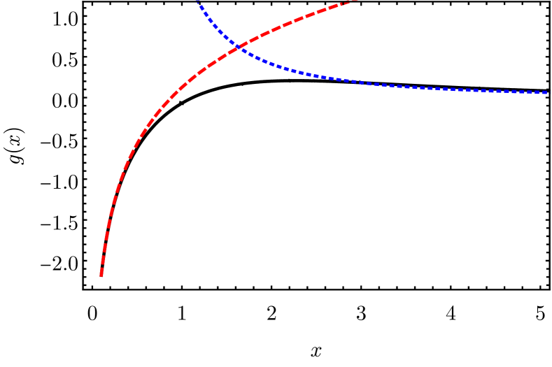
Figure S1: Function $g(x)$ given by Eq. (S26) (black solid curve) and its asymptotes Eq. (S27) (red dashed curve) and Eq. (S28) (blue dotted curve).

At relatively high temperatures $T\sim\Gamma$ one has to use Eq. (S20) to calculate the Green’s functions.

S3 S3. Calculation of spin susceptibility

To calculate the current induced spin accumulation in the QD, we write the electric current of the given spin component to the QD from the left/right leads [2]:

$$J_{\pm}^{L/R}=e\int\frac{\mathrm{d}\omega}{2\pi}\left[{\rm i}\Gamma_{\pm}^{L/R}G_{\pm}^{<}-2f_{L/R}\Gamma_{\pm}^{L/R}\mathop{\rm Im}G_{\pm}^{R}\right],$$ (S29)

where $G_{\pm}^{<}$ are the lesser Green’s functions of the QD. In the steady state, due to the spin and charge conservation in the QD, we have

$$J_{\pm}^{L}+J_{\pm}^{R}=0.$$ (S30)

From this relation we obtain the occupancies of the spin states of the QD in the form

$$\left\langle n_{\pm}\right\rangle=-{\rm i}\int\frac{\mathrm{d}\omega}{2\pi}G_{\pm}^{<}\\ =-\int\frac{\mathrm{d}\omega}{\pi\Gamma}\left[f_{L}\Gamma_{\pm}^{L}+f_{R}\Gamma_{\pm}^{R}\right]\mathop{\rm Im}G_{\pm}^{R}.$$ (S31)

These occupancies define the spin polarization in the QD even beyond the linear response regime.

We note that the lesser Green’s functions can be also calculated using the analytical continuation method [4, 5, 2] following the approach of Refs. 6, 7. However, the phenomenological truncation of the Heisenberg equations using the relations (S11) and (S13) yields in this way the Green’s functions $G_{\pm}^{<}$ that do not coincide with $-2{\rm i}f_{L/R}G_{\pm}^{R}$ in the equilibrium. Therefore, for consistency we prefer to determine the occupancies of the QD states from the charge and spin conservation relations (S30).

From Eq. (S23) one can see that Eq. (S31) can be rewritten as

$$\left\langle n_{\pm}\right\rangle=I_{\pm}(1-\left\langle n_{\mp}\right\rangle),$$ (S32)

where

$$I_{\pm}=-\int\frac{\mathrm{d}\omega}{\pi\Gamma}\left[f_{L}\Gamma_{\pm}^{L}+f_{R}\Gamma_{\pm}^{R}\right]\mathop{\rm Im}\frac{1}{\omega-E_{0}-\Sigma_{0}^{R}-\Sigma_{1,\pm}^{R}}$$ (S33)

do not depend on $\left\langle n_{\pm}\right\rangle$ (here we take into account that for finite $W$ Eq. (S18) may be weakly violated). From the solution of these equations we obtain the spin polarization in the QD

$$P\equiv\frac{\left\langle n_{+}-n_{-}\right\rangle}{\left\langle n_{+}+n_{-}\right\rangle}=\frac{I_{+}-I_{-}}{I_{+}+I_{-}-2I_{+}I_{-}}$$ (S34)

and its occupancy

$$\left\langle n_{+}+n_{-}\right\rangle=\frac{I_{+}+I_{-}-2I_{+}I_{-}}{1-I_{+}I_{-}}.$$ (S35)

These expressions generally define the spin state of the QD.

To calculate the spin susceptibility, we consider the symmetrically applied bias $eV$: $E_{F}^{L}=E_{F}+eV/2$, $E_{F}^{R}=E_{F}-eV/2$ and set $E_{F}=0$ to be specific. In the case of $eV=0$ one has $I_{+}=I_{-}=I_{0}$, where

$$I_{0}=-\int\frac{\mathrm{d}\omega}{\pi}\mathop{\rm Im}\frac{f_{0}(\omega)}{\omega-E_{0}-\Sigma_{0}^{R}-\Sigma_{1,0}^{R}}$$ (S36)

with

$$f_{0}(E)=\frac{1}{1+\exp\left[(E-E_{F})/T\right]}$$ (S37)

and

$$\Sigma_{1,0}^{R}=\Gamma\int\limits_{-W}^{W}\frac{\mathrm{d}E}{\pi}\frac{f_{0}(E)}{\omega-E+{\rm i}0}.$$ (S38)

In the first order in $eV$ we obtain

$$I_{+}-I_{-}=-\mathcal{C}\int\frac{\mathrm{d}\omega}{\pi}\mathop{\rm Im}\left[\frac{f_{L}(\omega)-f_{R}(\omega)}{\omega-E_{0}-\Sigma_{0}^{R}-\Sigma_{1,0}^{R}}\right.\\ \left.-\frac{\Gamma f_{0}(\omega)}{(\omega-E_{0}-\Sigma_{0}^{R}-\Sigma_{1,0}^{R})^{2}}\int\limits_{-W}^{W}\frac{\mathrm{d}E}{\pi}\frac{f_{L}(E)-f_{R}(E)}{\omega-E+{\rm i}0}\right].$$ (S39)

Then the spin susceptibility is given by

$$\chi_{s}=\frac{(I_{+}-I_{-})/(eV)}{2I_{0}(1-I_{0})}.$$ (S40)

From Eq. (S39) one can see that it linearly depends on the chirality $\mathcal{C}$, so we focus on the case of $\mathcal{C}=1$ in what follows and in the main text.

S4 S4. Estimation of spin susceptibility

To obtain a qualitative understanding of the current induced spin accumulation enhancement due to Kondo effect, we derive an analytical approximation for the spin susceptibility at low temperatures, $T_{K}<T\ll\Gamma$ and at high Fermi level $E_{F}-E_{0}\gg\Gamma$.

First of all, we note that in this limit $\left\langle n_{+}+n_{-}\right\rangle\approx 1$ because of the strong Coulomb interaction, so from Eq. (S35) we obtain $I_{0}\approx 1$. Then we note that the denominator in Eq. (S40) is close to zero, so the spin susceptibility $\chi_{s}$ is large. This is related to the fact that for the large Coulomb interaction the system is a sort of unstable: a small occupancy of one spin state strongly suppresses occupancy of another at the same moment.

To estimate $1-I_{0}$ we approximate Eq. (S36) as follows:

$$I_{0}\approx-\int\limits_{-W}^{E_{F}}\frac{\mathrm{d}\omega}{\pi}\mathop{\rm Im}\frac{1}{\omega-E_{0}+{\rm i}\Gamma}\\ =\frac{1}{\pi}\left[\mathop{\mathrm{arctg}}\left(\frac{W+E_{0}}{\Gamma}\right)+\mathop{\mathrm{arctg}}\left(\frac{E_{F}-E_{0}}{\Gamma}\right)\right].$$ (S41)

Then we rewrite Eq. (S33) for the case of $\mathcal{C}=1$ as

$$I_{+/-}=-\int\frac{\mathrm{d}\omega}{\pi}\mathop{\rm Im}\frac{f_{L/R}}{\omega-E_{0}-\Sigma_{0}^{R}-\Sigma_{1,+/-}^{R}}.$$ (S42)

Further from Eqs. (S10) and (S20) we obtain

$$\mathop{\rm Im}\Sigma_{0}^{R}=-\Gamma,\qquad\mathop{\rm Im}\Sigma_{1,+/-}^{R}=-\Gamma f_{R/L},$$ (S43)

thus we arrive at

$$I_{+/-}=\int\frac{\mathrm{d}\omega}{\pi}\frac{\Gamma f_{L/R}(1+f_{R/L})}{\left|\omega-E_{0}-\Sigma_{0}^{R}-\Sigma_{1,+/-}^{R}\right|^{2}}.$$ (S44)

Next we separate the three contributions to the current induced spin accumulation as follows [cf. Eq. (S39)]:

$$I_{+}-I_{-}=\Delta I_{1}+\Delta I_{2}+\Delta I_{3},$$ (S45)

where

$$\Delta I_{1}=\int\frac{\mathrm{d}\omega}{\pi}\frac{\Gamma(f_{L}-f_{R})}{\left|\omega-E_{0}-\Sigma_{0}^{R}-\Sigma_{1,0}^{R}\right|^{2}},$$ (S46a)

$$\Delta I_{2}=\int\frac{\mathrm{d}\omega}{\pi}\frac{2\Gamma^{3}(f_{L}-f_{R})f_{0}(1+f_{0})^{2}}{\left|\omega-E_{0}-\Sigma_{0}^{R}-\Sigma_{1,0}^{R}\right|^{4}},$$ (S46b)

$$\Delta I_{3}=\int\frac{\mathrm{d}\omega}{\pi}2\Gamma^{2}f_{0}(1+f_{0})\mathop{\rm Re}(\Sigma_{1,+}^{R}-\Sigma_{1,-}^{R})\\ \times\frac{\mathop{\rm Re}(\omega-E_{0}-\Sigma_{0}^{R}-\Sigma_{1,0}^{R})}{\left|\omega-E_{0}-\Sigma_{0}^{R}-\Sigma_{1,0}^{R}\right|^{4}}.$$ (S46c)

In the first two contributions, we replace $f_{L}-f_{R}$ with $eV\delta(\omega-E_{F})$ and note that at $\omega=E_{F}$ it follows from Eqs. (S24) and (S27) that

$$\Sigma_{1,0}^{R}=\frac{\Gamma}{\pi}\left[\ln\left(\frac{2W}{\pi T}\right)+\gamma\right]-{\rm i}\frac{\Gamma}{2}$$ (S47)

and taking into account Eq. (S18) we obtain

$$\Delta I_{1}=\frac{eV}{\pi}\frac{\Gamma}{a^{2}+(3\Gamma/2)^{2}},$$ (S48)

$$\Delta I_{2}=\frac{eV}{\pi}\frac{9\Gamma^{3}}{4\left[a^{2}+(3\Gamma/2)^{2}\right]^{2}},$$ (S49)

where

$$a=\left|E_{F}-E_{0}-\frac{\Gamma}{\pi}\left[\ln\left(\frac{2W}{\pi T}\right)+\gamma\right]\right|.$$ (S50)

Finally, we estimate the last contribution as

$$\Delta I_{3}=h(W/T)-h(W/\Gamma),$$ (S51)

where

$$h(x)=\frac{2/\pi}{\frac{(E_{F}-E_{0})^{2}}{\Gamma^{2}}+4-\frac{2(E_{F}-E_{0})}{\pi\Gamma}\ln(x)+\ln^{2}(x)}.$$ (S52)

Now the analytical estimation for the spin susceptibility is given by Eqs. (S40), (S41), (S45), (S48), (S49), and (S51). It is shown by the gray dotted line in Fig. 3(a) in the main text.

To find an order of magnitude estimation we note that

$$1-I_{0}\sim\frac{\Gamma}{E_{F}-E_{0}},\quad\Delta I_{1,2,3}\sim\frac{eV}{\Gamma}.$$ (S53)

So Eq. (S40) yields [Eq. (9) in the main text]

$$\chi_{s}\sim\frac{E_{F}-E_{0}}{\Gamma^{2}}.$$ (S54)

For comparison, in the Hartree-Fock approximation we obtain in the same way from Eq. (S19) that the occupancies of the spin states obey the equations [3]

$$\left\langle n_{+/-}\right\rangle=\frac{1}{\pi}\int\limits_{-W}^{W}\frac{\Gamma(1-\left\langle n_{-/+}\right\rangle)^{2}f_{L/R}}{(\omega-E_{0})^{2}+\Gamma^{2}(1-\left\langle n_{-/+}\right\rangle)^{2}}\mathrm{d}\omega.$$ (S55)

These equations should be solved self consistently for $\left\langle n_{\pm}\right\rangle$. They were used to calculate the spin susceptibility $\chi_{s}^{(0)}$ for Fig. 3 in the main text.

In the wide band limit ($W\to\infty$) and for the large Fermi energy ($E_{F}-E_{0}\gg\Gamma,T$), Eq. (S55) can be written in the form of Eq. (S32) with

$$I_{\pm}=1-\frac{\Gamma/\pi}{E_{F}-E_{0}}\pm\frac{\Gamma eV}{2\pi(E_{F}-E_{0})^{2}}.$$ (S56)

Thus, using Eq. (S40) we find an estimation for the spin susceptibility in the Hartree-Fock approximation:

$$\chi_{s}^{(0)}\sim\frac{1}{E_{F}-E_{0}}.$$ (S57)

As discussed in the main text, it is parametrically smaller than the spin susceptibility at low temperatures with account for the many body correlations [Eq. (S54)]. The reason for this is the absence of the peak in the density of states at the Fermi energy and underestimation of the role of the Coulomb interaction.

References

- Michler [2017] P. Michler, Quantum dots for quantum information technologies, Vol. 237 (Springer, 2017).
- Kloeffel and Loss [2013] C. Kloeffel and D. Loss, Prospects for Spin-Based Quantum Computing in Quantum Dots, Annu. Rev. Condens. Matter. Phys. 4, 51 (2013).
- Watson et al. [2018] T. F. Watson, S. G. J. Philips, E. Kawakami, D. R. Ward, P. Scarlino, M. Veldhorst, D. E. Savage, M. G. Lagally, M. Friesen, S. N. Coppersmith, M. A. Eriksson, and L. M. K. Vandersypen, A programmable two-qubit quantum processor in silicon, Nature 555, 633 (2018).
- Yoneda et al. [2018] J. Yoneda, K. Takeda, T. Otsuka, T. Nakajima, M. R. Delbecq, G. Allison, T. Honda, T. Kodera, S. Oda, Y. Hoshi, N. Usami, K. M. Itoh, and S. Tarucha, A quantum-dot spin qubit with coherence limited by charge noise and fidelity higher than 99.9%, Nat. Nanotechnol. 13, 102 (2018).
- Yang et al. [2020] C. H. Yang, R. C. C. Leon, J. C. C. Hwang, A. Saraiva, T. Tanttu, W. Huang, J. Camirand Lemyre, K. W. Chan, K. Y. Tan, F. E. Hudson, K. M. Itoh, A. Morello, M. Pioro-Ladriére, A. Laucht, and A. S. Dzurak, Operation of a silicon quantum processor unit cell above one kelvin, Nature 580, 350 (2020).
- Bracker et al. [2005] A. S. Bracker, E. A. Stinaff, D. Gammon, M. E. Ware, J. G. Tischler, A. Shabaev, A. L. Efros, D. Park, D. Gershoni, V. L. Korenev, and I. A. Merkulov, Optical Pumping of the Electronic and Nuclear Spin of Single Charge-Tunable Quantum Dots, Phys. Rev. Lett. 94, 047402 (2005).
- Xu et al. [2007] X. Xu, Y. Wu, B. Sun, Q. Huang, J. Cheng, D. G. Steel, A. S. Bracker, D. Gammon, C. Emary, and L. J. Sham, Fast Spin State Initialization in a Singly Charged InAs-GaAs Quantum Dot by Optical Cooling, Phys. Rev. Lett. 99, 097401 (2007).
- Gerardot et al. [2008] B. D. Gerardot, D. Brunner, P. A. Dalgarno, P. Ohberg, S. Seidl, M. Kroner, K. Karrai, N. G. Stoltz, P. M. Petroff, and R. J. Warburton, Optical pumping of a single hole spin in a quantum dot, Nature 451, 441 (2008).
- Greilich et al. [2006] A. Greilich, R. Oulton, E. A. Zhukov, I. A. Yugova, D. R. Yakovlev, M. Bayer, A. Shabaev, A. L. Efros, I. A. Merkulov, V. Stavarache, D. Reuter, and A. Wieck, Optical Control of Spin Coherence in Singly Charged (In,Ga)As/GaAs Quantum Dots, Phys. Rev. Lett. 96, 227401 (2006).
- Press et al. [2008] D. Press, T. D. Ladd, B. Zhang, and Y. Yamamoto, Complete quantum control of a single quantum dot spin using ultrafast optical pulses, Nature (London) 456, 218 (2008).
- Greilich et al. [2009] A. Greilich, S. E. Economou, S. Spatzek, D. R. Yakovlev, D. Reuter, A. D. Wieck, T. L. Reinecke, and M. Bayer, Ultrafast optical rotations of electron spins in quantum dots, Nat. Phys. 5, 262 (2009).
- Dusanowski et al. [2022] Ł. Dusanowski, C. Nawrath, S. L. Portalupi, M. Jetter, T. Huber, S. Klembt, P. Michler, and S. Höfling, Optical charge injection and coherent control of a quantum-dot spin-qubit emitting at telecom wavelengths, Nat. Commun. 13, 748 (2022).
- Berezovsky et al. [2006] J. Berezovsky, M. H. Mikkelsen, O. Gywat, N. G. Stoltz, L. A. Coldren, and D. D. Awschalom, Nondestructive optical measurements of a single electron spin in a quantum dot, Science 314, 1916 (2006).
- Atature et al. [2007] M. Atature, J. Dreiser, A. Badolato, and A. Imamoglu, Observation of Faraday rotation from a single confined spin, Nat. Phys. 3, 101 (2007).
- Arnold et al. [2015] C. Arnold, J. Demory, V. Loo, A. Lemaitre, I. Sagnes, M. Glazov, O. Krebs, P. Voisin, P. Senellart, and L. Lanco, Macroscopic rotation of photon polarization induced by a single spin, Nat. Commun. 6, 6236 (2015).
- Nowack et al. [2007] K. C. Nowack, F. H. L. Koppens, Y. V. Nazarov, and L. M. K. Vandersypen, Coherent Control of a Single Electron Spin with Electric Fields, Science 318, 1430 (2007).
- Shchepetilnikov et al. [2016] A. V. Shchepetilnikov, D. D. Frolov, Y. A. Nefyodov, I. V. Kukushkin, D. S. Smirnov, L. Tiemann, C. Reichl, W. Dietsche, and W. Wegscheider, Nuclear magnetic resonance and nuclear spin relaxation in AlAs quantum well probed by ESR, Phys. Rev. B 94, 241302(R) (2016).
- Zajac et al. [2018] D. M. Zajac, A. J. Sigillito, M. Russ, F. Borjans, J. M. Taylor, G. Burkard, and J. R. Petta, Resonantly driven CNOT gate for electron spins, Science 359, 439 (2018).
- Mills et al. [2019] A. R. Mills, D. M. Zajac, M. J. Gullans, F. J. Schupp, T. M. Hazard, and J. R. Petta, Shuttling a single charge across a one-dimensional array of silicon quantum dots, Nat. Commun. 10, 1063 (2019).
- Qiao et al. [2021] H. Qiao, Y. P. Kandel, S. Fallahi, G. C. Gardner, M. J. Manfra, X. Hu, and J. M. Nichol, Long-Distance Superexchange between Semiconductor Quantum-Dot Electron Spins, Phys. Rev. Lett. 126, 017701 (2021).
- Carter et al. [2021] S. G. Carter, S. C. Badescu, A. S. Bracker, M. K. Yakes, K. X. Tran, J. Q. Grim, and D. Gammon, Coherent Population Trapping Combined with Cycling Transitions for Quantum Dot Hole Spins Using Triplet Trion States, Phys. Rev. Lett. 126, 107401 (2021).
- Dyakonov [2017] M. I. Dyakonov, ed., Spin physics in semiconductors (Springer International Publishing AG, Berlin, 2017).
- Ivchenko and Pikus [1978] E. L. Ivchenko and G. E. Pikus, New photogalvanic effect in gyrotropic crystals, JETP Lett. 27, 604 (1978).
- Vorob’ev et al. [1979] L. E. Vorob’ev, E. L. Ivchenko, G. E. Pikus, I. I. Farbshtein, V. A. Shalygin, and A. V. Shturbin, Optical activity in tellurium induced by a current, JETP Lett. 29, 441 (1979).
- Kato et al. [2004] Y. K. Kato, R. C. Myers, A. C. Gossard, and D. D. Awschalom, Current-Induced Spin Polarization in Strained Semiconductors, Phys. Rev. Lett. 93, 176601 (2004).
- Ganichev et al. [2006] S. D. Ganichev, S. N. Danilov, P. Schneider, V. V. Bel’kov, L. E. Golub, W. Wegscheider, D. Weiss, and W. Prettl, Electric current-induced spin orientation in quantum well structures, J. Magn. Magn. Mater. 300, 127 (2006).
- Silov et al. [2004] A. Y. Silov, P. A. Blajnov, J. H. Wolter, R. Hey, K. H. Ploog, and N. S. Averkiev, Current-induced spin polarization at a single heterojunction, Appl. Phys. Lett. 85, 5929 (2004).
- Yang et al. [2021] S.-H. Yang, R. Naaman, Y. Paltiel, and S. S. P. Parkin, Chiral spintronics, Nat. Rev. Phys. 3, 328 (2021).
- Kim et al. [2021] Y.-H. Kim, Y. Zhai, H. Lu, X. Pan, C. Xiao, E. A. Gaulding, S. P. Harvey, J. J. Berry, Z. V. Vardeny, J. M. Luther, and M. C. Beard, Chiral-induced spin selectivity enables a room-temperature spin light-emitting diode, Science 371, 1129 (2021).
- Evers et al. [2022] F. Evers, A. Aharony, N. Bar-Gill, O. Entin-Wohlman, P. Hedegård, O. Hod, P. Jelinek, G. Kamieniarz, M. Lemeshko, K. Michaeli, V. Mujica, R. Naaman, Y. Paltiel, S. Refaely-Abramson, O. Tal, J. Thijssen, M. Thoss, J. M. van Ruitenbeek, L. Venkataraman, D. H. Waldeck, B. Yan, and L. Kronik, Theory of Chirality Induced Spin Selectivity: Progress and Challenges, Adv. Mater. 34, 2106629 (2022).
- Ganichev et al. [2012] S. D. Ganichev, M. Trushin, and J. Schliemann, Spin polarization by current in Handbook of Spin Transport and Magnetism, edited by E. Y, Tsymbal and I. Zutic, p. 487 (Chapman & Hall, Boca Raton, 2012).
- Li et al. [2016] C. H. Li, O. M. J. van’t Erve, S. Rajput, L. Li, and B. T. Jonker, Direct comparison of current-induced spin polarization in topological insulator Bi2Se3 and InAs Rashba states, Nat. Commun. 7, 13518 (2016).
- Vaklinova et al. [2016] K. Vaklinova, A. Hoyer, M. Burghard, and K. Kern, Current-Induced Spin Polarization in Topological Insulator–Graphene Heterostructures, Nano Lett. 16, 2595 (2016).
- Tian et al. [2017] J. Tian, S. Hong, I. Miotkowski, S. Datta, and Y. P. Chen, Observation of current-induced, long-lived persistent spin polarization in a topological insulator: A rechargeable spin battery, Sci. Adv. 3, e1602531 (2017).
- Golub and Ivchenko [2013] L. E. Golub and E. L. Ivchenko, Spin-dependent phenomena in semiconductors in strong electric fields, New J. Phys. 15, 125003 (2013).
- Golub and Ivchenko [2014] L. E. Golub and E. L. Ivchenko (Nova Science Publishers, 2014) pp. 93–104.
- Smirnov and Golub [2017] D. S. Smirnov and L. E. Golub, Electrical Spin Orientation, Spin-Galvanic, and Spin-Hall Effects in Disordered Two-Dimensional Systems, Phys. Rev. Lett. 118, 116801 (2017).
- Shumilin et al. [2016] A. V. Shumilin, E. Y. Sherman, and M. M. Glazov, Spin dynamics of hopping electrons in quantum wires: Algebraic decay and noise, Phys. Rev. B 94, 125305 (2016).
- Murakami et al. [2003] S. Murakami, N. Nagaosa, and S.-C. Zhang, Dissipationless Quantum Spin Current at Room Temperature, Science 301, 1348 (2003).
- Mantsevich and Smirnov [2022] V. N. Mantsevich and D. S. Smirnov, Current-induced hole spin polarization in a quantum dot via a chiral quasi bound state, Nanoscale Horiz. 7, 752 (2022).
- Sinova et al. [2015] J. Sinova, S. O. Valenzuela, J. Wunderlich, C. Back, and T. Jungwirth, Spin Hall effects, Rev. Mod. Phys. 87, 1213 (2015).
- Abakumov and Yassievich [1972] V. Abakumov and I. Yassievich, Anomalous Hall Effect for Polarized Electrons in Semiconductors, JETP 34, 1375 (1972).
- Hewson [1997] A. C. Hewson, The Kondo problem to heavy fermions (Cambridge university press, Cambridge, UK, 1997).
- Krishna-murthy et al. [1980] H. R. Krishna-murthy, J. W. Wilkins, and K. G. Wilson, Renormalization-group approach to the Anderson model of dilute magnetic alloys. II. Static properties for the asymmetric case, Phys. Rev. B 21, 1044 (1980).
- Anderson [1961] P. W. Anderson, Localized Magnetic States in Metals, Phys. Rev. 124, 41 (1961).
- Lodahl et al. [2017] P. Lodahl, S. Mahmoodian, S. Stobbe, A. Rauschenbeutel, P. Schneeweiss, J. Volz, H. Pichler, and P. Zoller, Chiral quantum optics, Nature 541, 473 (2017).
- Dyakov et al. [2018] S. A. Dyakov, V. A. Semenenko, N. A. Gippius, and S. G. Tikhodeev, Magnetic field free circularly polarized thermal emission from a chiral metasurface, Phys. Rev. B 98, 235416 (2018).
- Spitzer et al. [2018] F. Spitzer, A. N. Poddubny, I. A. Akimov, V. F. Sapega, L. Klompmaker, L. E. Kreilkamp, L. V. Litvin, R. Jede, G. Karczewski, M. Wiater, T. Wojtowicz, D. R. Yakovlev, and M. Bayer, Routing the emission of a near-surface light source by a magnetic field, Nat. Phys. 14, 1043 (2018).
- Overvig et al. [2021] A. Overvig, N. Yu, and A. Alù, Chiral Quasi-Bound States in the Continuum, Phys. Rev. Lett. 126, 073001 (2021).
- Rammer and Smith [1986] J. Rammer and H. Smith, Quantum field-theoretical methods in transport theory of metals, Rev. Mod. Phys. 58, 323 (1986).
- Stefanucci and van Leeuwen [2013] G. Stefanucci and R. van Leeuwen, Nonequilibrium Many-Body Theory of Quantum Systems: A Modern Introduction (Cambridge University Press, 2013).
- Arseev [2015] P. I. Arseev, On the nonequilibrium diagram technique: derivation, some features, and applications, Phys. Usp. 58, 1159 (2015).
- Kashcheyevs et al. [2006] V. Kashcheyevs, A. Aharony, and O. Entin-Wohlman, Applicability of the equations-of-motion technique for quantum dots, Phys. Rev. B 73, 125338 (2006).
- Lacroix [1981] C. Lacroix, Density of states for the Anderson model, J. Phys. F 11, 2389 (1981).
- Meir et al. [1993] Y. Meir, N. S. Wingreen, and P. A. Lee, Low-temperature transport through a quantum dot: The Anderson model out of equilibrium, Phys. Rev. Lett. 70, 2601 (1993).
- Świrkowicz et al. [2003] R. Świrkowicz, J. Barnaś, and M. Wilczyński, Nonequilibrium Kondo effect in quantum dots, Phys. Rev. B 68, 195318 (2003).
- Haug and Jauho [2008] H. Haug and A.-P. Jauho, Quantum kinetics in transport and optics of semiconductors, Vol. 2 (Springer, 2008).
- [58] See Supplemental Material, which includes Refs. 66, 67, 68, for details on the derivation of the Green’s functions, wide band approximation, calculation of the spin susceptibility, and its estimation.
- Žitko and Bonča [2011] R. Žitko and J. Bonča, Kondo effect in the presence of Rashba spin-orbit interaction, Phys. Rev. B 84, 193411 (2011).
- Zarea et al. [2012] M. Zarea, S. E. Ulloa, and N. Sandler, Enhancement of the Kondo Effect through Rashba Spin-Orbit Interactions, Phys. Rev. Lett. 108, 046601 (2012).
- Wong et al. [2016] A. Wong, S. E. Ulloa, N. Sandler, and K. Ingersent, Influence of Rashba spin-orbit coupling on the Kondo effect, Phys. Rev. B 93, 075148 (2016).
- Debray et al. [2009] P. Debray, S. M. S. Rahman, J. Wan, R. S. Newrock, M. Cahay, A. T. Ngo, S. E. Ulloa, S. T. Herbert, M. Muhammad, and M. Johnson, All-electric quantum point contact spin-polarizer, Nat. Nanotech. 4, 759 (2009).
- Chuang et al. [2015] P. Chuang, S.-C. Ho, L. W. Smith, F. Sfigakis, M. Pepper, C.-H. Chen, J.-C. Fan, J. P. Griffiths, I. Farrer, H. E. Beere, G. A. C. Jones, D. A. Ritchie, and T.-M. Chen, All-electric all-semiconductor spin field-effect transistors, Nat. Nanotech. 10, 35 (2015).
- Härtl et al. [2023] P. Härtl, M. Leisegang, J. Kügel, and M. Bode, Probing spin-dependent charge transport at single-nanometer length scales (2023), arXiv:2303.00393 .
- Smith et al. [2022] L. W. Smith, H.-B. Chen, C.-W. Chang, C.-W. Wu, S.-T. Lo, S.-H. Chao, I. Farrer, H. E. Beere, J. P. Griffiths, G. A. C. Jones, D. A. Ritchie, Y.-N. Chen, and T.-M. Chen, Electrically Controllable Kondo Correlation in Spin-Orbit-Coupled Quantum Point Contacts, Phys. Rev. Lett. 128, 027701 (2022).
- Langreth [1976] D. C. Langreth, Linear and Nonlinear Response Theory with Applications, in Linear and Nonlinear Electron Transport in Solids, edited by J. T. Devreese and V. E. van Doren (Springer US, Boston, MA, 1976) pp. 3–32.
- Niu et al. [1999] C. Niu, D. L. Lin, and T.-H. Lin, Equation of motion for nonequilibrium Green functions, J. Phys.: Cond. Mat. 11, 1511 (1999).
- Kadanoff and Baym [2018] L. P. Kadanoff and G. Baym, Quantum statistical mechanics: Green’s function methods in equilibrium and nonequilibrium problems (CRC Press, 2018).

References

- Meir et al. [1993] Y. Meir, N. S. Wingreen, and P. A. Lee, Low-temperature transport through a quantum dot: The Anderson model out of equilibrium, Phys. Rev. Lett. 70, 2601 (1993).
- Haug and Jauho [2008] H. Haug and A.-P. Jauho, Quantum kinetics in transport and optics of semiconductors, Vol. 2 (Springer, 2008).
- Mantsevich and Smirnov [2022] V. N. Mantsevich and D. S. Smirnov, Current-induced hole spin polarization in a quantum dot via a chiral quasi bound state, Nanoscale Horiz. 7, 752 (2022).
- Langreth [1976] D. C. Langreth, Linear and Nonlinear Response Theory with Applications, in Linear and Nonlinear Electron Transport in Solids, edited by J. T. Devreese and V. E. van Doren (Springer US, Boston, MA, 1976) pp. 3–32.
- Kadanoff and Baym [2018] L. P. Kadanoff and G. Baym, Quantum statistical mechanics: Green’s function methods in equilibrium and nonequilibrium problems (CRC Press, 2018).
- Niu et al. [1999] C. Niu, D. L. Lin, and T.-H. Lin, Equation of motion for nonequilibrium Green functions, J. Phys.: Cond. Mat. 11, 1511 (1999).
- Świrkowicz et al. [2003] R. Świrkowicz, J. Barnaś, and M. Wilczyński, Nonequilibrium Kondo effect in quantum dots, Phys. Rev. B 68, 195318 (2003).