Quasi Maximum Likelihood Estimation of High-Dimensional Factor Models:
A Critical Review

Abstract

We review Quasi Maximum Likelihood estimation of factor models for high-dimensional panels of time series. We consider two cases: (1) estimation when no dynamic model for the factors is specified (Bai and Li, 2012, 2016); (2) estimation based on the Kalman smoother and the Expectation Maximization algorithm thus allowing to model explicitly the factor dynamics (Doz et al., 2012; Barigozzi and Luciani, 2019). Our interest is in approximate factor models, i.e., when we allow for the idiosyncratic components to be mildly cross-sectionally, as well as serially, correlated. Although such setting apparently makes estimation harder, we show, in fact, that factor models do not suffer of the curse of dimensionality problem, but instead they enjoy a blessing of dimensionality property. In particular, given an approximate factor structure, if the cross-sectional dimension of the data, $N$, grows to infinity, we show that: (i) identification of the model is still possible, (ii) the mis-specification error due to the use of an exact factor model log-likelihood vanishes. Moreover, if we let also the sample size, $T$, grow to infinity, we can also consistently estimate all parameters of the model and make inference. The same is true for estimation of the latent factors which can be carried out by weighted least-squares, linear projection, or Kalman filtering/smoothing. We also compare the approaches presented with: Principal Component analysis and the classical, fixed $N$, exact Maximum Likelihood approach. We conclude with a discussion on efficiency of the considered estimators.

Keywords: Approximate Dynamic Factor Model; Maximum Likelihood Estimation; Weighted Least Squares; Expectation Maximization Algorithm; Kalman smoother.

1 Introduction

Factor analysis is one of the earliest proposed multivariate statistical techniques: it dates back to the studies of Spearman (1904) in experimental psychology. The idea is to decompose a vector of $N$ observed random variables into two components: (i) a common component driven by $r<N$ latent factors, and (ii) a component which is idiosyncratic, in the sense that it can be due either to measurement errors or to specific features of a single, or a sub-group of variables. As such we can retrospectively consider factor analysis as a pioneering technique in the filed of unsupervised statistical learning.

Over the years, two main strands of applications have emerged: first, in psychometrics in a low-dimensional setting (Thomson, 1936; Bartlett, 1937, 1938; Lawley, 1940; Thomson, 1951; Jöreskog, 1969; Lawley and Maxwell, 1971; Moustaki and Knott, 2000; Jöreskog and Moustaki, 2001; Bartholomew et al., 2011), second, in econometrics, both in a low-dimensional (Sargent and Sims, 1977; Geweke and Singleton, 1981; Watson and Engle, 1983; Stock and Watson, 1989, 1991), and in a high-dimensional setting (Chamberlain and Rothschild, 1983; Forni et al., 2000; Stock and Watson, 2002a; Bai, 2003). Applications in econometrics include: the analysis of financial markets (Connor et al., 2006; Aït-Sahalia and Xiu, 2017; Kim and Fan, 2019; Barigozzi and Hallin, 2020), the measurement and prediction of macroeconomic aggregates (Stock and Watson, 2002b; De Mol et al., 2008; Giannone et al., 2008; Barigozzi and Luciani, 2021), the study of the dynamic effects of unexpected shocks to the economy (Bernanke et al., 2005; Forni et al., 2009; Forni and Gambetti, 2010; Barigozzi et al., 2014; Forni et al., 2014; Luciani, 2015; Marcellino and Sivec, 2016; Barigozzi et al., 2021), and the analysis of demand systems (Stone, 1945; Barigozzi and Moneta, 2016). An historical overview is in Barigozzi and Hallin (2024).

The former strand of literature deals with random samples of data, i.e., independent observations for each variable, and estimation is almost exclusively by means of Maximum Likelihood (Anderson and Rubin, 1956; Amemiya et al., 1987; Anderson and Amemiya, 1988; Tipping and Bishop, 1999; Bai and Li, 2012). The latter strand of literature deals with time series data, i.e., dependent observations for each variable, and estimation is either by means of Principal Component analysis (Forni et al., 2000; Stock and Watson, 2002a; Bai, 2003; Fan et al., 2013) or by means of Quasi Maximum Likelihood (Quah and Sargent, 1993; Doz et al., 2012; Bai and Li, 2016). Principal Components and Quasi Maximum Likelihood estimation are the most popular estimation techniques, dating back at least to Hotelling (1933) and Lawley (1940), respectively. A third, less popular, approach is the centroid method by Thomson (1951).

Our focus is on high-dimensional factor models for time series. Specifically, we allow for the dimension of the vector, $N$, to grow to infinity. As a consequence, it is realistic to consider an approximate factor model where we allow for the idiosyncratic components to be cross-sectionally correlated, rather than an exact factor model where the idiosyncratic components are not correlated. Furthermore, since we deal with time series, both the factors and the idiosyncratic components are allowed to be autocorrelated, and, if we specify also a model describing the time evolution of the factors, e.g., a VAR, we speak of a dynamic factor model, while, if we do not, we speak of a static factor model. The approximate dynamic factor model considered in this paper is a restricted version of the more general model proposed by Forni et al. (2000).

The idea of an approximate factor structure dates back to Chamberlain and Rothschild (1983) who showed that, if we let the number of time series, $N$, to grow, then we are able to identify the common components even when allowing for idiosyncratic correlations. Intuitively, since estimation is based on cross-sectional aggregation, the more series we use, i.e., the more we increase $N$, the more the signal, factor-driven, component emerges from the noisy idiosyncratic component because of an assumed cross-sectional weak Law of Large Numbers. Equivalently, this is seen by noticing that, under a factor model, the gap between the largest $r$ eigenvalues of the covariance matrix of the data and the remaining $N-r$ widens as $N$ grows. As a consequence of this phenomenon, an approximate factor model does not suffer of the curse of dimensionality problem, which typically affects high-dimensional parametric models, but it enjoys instead a blessing of dimensionality property.

The idea of a dynamic factor model goes back to Sargent and Sims (1977), who account for the possibility that the $N$ variables co-move not only contemporaneously but also with some leads or lags, in other words, they can load the factors also with lags. In particular, the setting considered here is the same as the one formulated by Forni et al. (2009), which consists in writing the model as a linear state-space system, having as latent states the factors.

In this paper, we review likelihood-based methods for estimating high-dimensional approximate static and dynamic factor models, as considered by Bai and Li (2016) and Doz et al. (2012), respectively. On the one hand, Bai and Li (2016) treat the factors as non-stochastic and follow the classical approach based on first estimating the loadings and the idiosyncratic variances by Quasi Maximum Likelihood and then estimating the factors by Weighted Least Squares. On the other hand, Doz et al. (2012) explicitly model the factors as an autocorrelated stochastic process and propose to use the Expectation Maximization (EM) algorithm together with the Kalman smoother to obtain joint estimates of the loadings and the idiosyncratic variances, which approximate the Quasi Maximum Likelihood estimators, and of the factors. Both approaches are based on the maximization of a mis-specified log-likelihood where we do not take into account any of the idiosyncratic cross- and serial correlations, nevertheless, we show that as $N\to\infty$, the mis-specification error vanishes: yet another instance of the blessing of dimensionality. A summary of the rates of convergence of the loadings and factors estimators in approximate and exact factor models is in Table 1.

Table 1: Rates of consistency of estimators of factor models

		Exact static factor model ($\bm{\Omega}^{F}=\mathbf{I}_{T}\otimes\bm{\Gamma}^{F}$, $\bm{\Omega}^{\xi}=\mathbf{I}_{T}\otimes\bm{\Sigma}^{\xi}$)
		Loadings ($\bm{\lambda}_{i}$)	Factors ($\mathbf{F}_{t}$)
$T\to\infty$	$n$ finite	$\sqrt{T}$	-
		Amemiya et al. (1987, Theorem 2F), QML
$T\to\infty$	$n\to\infty$	$\sqrt{T}$	$\min(\sqrt{n},T)$
		Bai and Li (2012, Theorem 5.2), QML	Bai and Li (2012, Theorem 6.1), WLS, LP
		Approximate static factor model ($\bm{\Omega}^{F}=\mathbf{I}_{T}\otimes\bm{\Gamma}^{F}$, $\bm{\Omega}^{\xi}$ unrestricted)
		Loadings ($\bm{\lambda}_{i}$)	Factors ($\mathbf{F}_{t}$)
$T\to\infty$	$n\to\infty$	$\min(n,\sqrt{T})$	$\min(\sqrt{n},T)$
		Bai (2003, Theorem 2), PC	Bai (2003, Theorem 1), PC
		Bai and Li (2016, Theorem 1), QML	Bai and Li (2016, Theorem 2), WLS, LP
		Approximate dynamic factor model ($\bm{\Omega}^{F}$, $\bm{\Omega}^{\xi}$ unrestricted)
		Loadings ($\bm{\lambda}_{i}$)	Factors ($\mathbf{F}_{t}$)
$T\to\infty$	$n\to\infty$	$\min(n/\sqrt{\log T},\sqrt{T})$	$\min(\sqrt{n},T/\sqrt{\log n})$
		Barigozzi and Luciani (2019, Proposition 2), EM	Barigozzi and Luciani (2019, Proposition 3), KS
			$\min(\sqrt{n/\log n},T^{1/4})$
			Doz et al. (2012, Proposition 1), KS

QML: Quasi Maximum Likelihood; PC: Principal Components; WLS: Weighted Least Squares; LP: Linear Projection; EM: Expectation Maximization Algorithm; KS: Kalman smoother. Here $\bm{\Gamma}^{F}$ and $\bm{\Sigma}^{\xi}$ are defined in Section 2.1 and $\bm{\Omega}^{F}$ and $\bm{\Omega}^{\xi}$ are defined in Section 4. In all cases the factors are estimated using the estimator of the loadings on the same row.

2 The approximate factor model

Let us consider the $T\times N$ double-array $\bm{X}$ having elements $\{x_{it}\in,\,i=1,\ldots,N,\,t=1,\ldots,T\}$ of $N$ observed times series over $T$ time periods. We say that $\bm{X}$ follows an $r$-factor model if

$$x_{it} =\alpha_{i}+\bm{\lambda}_{i}^{\prime}\mathbf{F}_{t}+\xi_{it},\quad i=1,\ldots,N,\quad t=1,\ldots,T.$$ (1)

where $\bm{\lambda}_{i}:=(\lambda_{i1}\cdots\lambda_{ir})^{\prime}$ and $\mathbf{F}_{t}:=(F_{1t}\cdots F_{rt})^{\prime}$ are the $r$-dimensional latent vectors of loadings for series $i$ and factors, respectively. We call $\xi_{it}$ the idiosyncratic component and $\chi_{it}:=\bm{\lambda}_{i}^{\prime}\mathbf{F}_{t}$ the common component.

It is convenient to write model (1), which is written is scalar notation, also in other equivalent ways which we list below.

Let $\mathbf{x}_{t}:=(x_{1t}\cdots x_{Nt})^{\prime}$ be the $N$-dimensional vector of observables at time $t$. Then, in vector notation (1) reads

$$\mathbf{x}_{t}=\bm{\alpha}+\bm{\Lambda}\mathbf{F}_{t}+\bm{\xi}_{t},\quad t=1\ldots,T,$$

where $\bm{\xi}_{t}:=(\xi_{1t}\cdots\xi_{Nt})^{\prime}$ is the corresponding $N$-dimensional vector of idiosyncratic components, $\bm{\Lambda}:=(\bm{\lambda}_{1}\cdots\bm{\lambda}_{N})^{\prime}=(\bm{\ell}_{1}\cdots\bm{\ell}_{r})$ is the $n\times r$ matrix of factor loadings with rows $\bm{\lambda}_{i}^{\prime}$, $i=1,\ldots,N$ and columns $\bm{\ell}_{j}$, $j=1,\ldots,r$, and $\bm{\alpha}:=(\alpha_{1}\cdots\alpha_{N})^{\prime}$. We call $\bm{\chi}_{t}:=\bm{\Lambda}\mathbf{F}_{t}$ the vector of common components.

Equivalently, let $\bm{x}_{i}:=(x_{i1}\cdots x_{iT})^{\prime}$ be the $T$-dimensional time series vector of the $i$th observable, in vector notation (1) also reads

$$\bm{x}_{i}=\alpha_{i}\bm{\iota}_{T}+\bm{F}\bm{\lambda}_{i}+\bm{\zeta}_{i},\quad i=1,\ldots,N,$$

where $\bm{\zeta}_{i}:=(\xi_{i1}\cdots\xi_{iT})^{\prime}$ is the corresponding $T$-dimensional time series vector of the $i$th idiosyncratic component, $\bm{F}:=(\mathbf{F}_{1}\cdots\mathbf{F}_{T})^{\prime}$ is the $T\times r$ matrix of factors, and $\bm{\iota}_{T}$ is a $T$-dimensional column vector of ones.

Finally, given that $\bm{X}=(\mathbf{x}_{1}\cdots\mathbf{x}_{T})^{\prime}$, in matrix notation (1) reads

$$\bm{X}=\bm{\iota}_{T}\bm{\alpha}^{\prime}+\bm{F}\bm{\Lambda}^{\prime}+\bm{\Xi},$$ (2)

where $\bm{\Xi}:=(\bm{\xi}_{1}\cdots\bm{\xi}_{T})^{\prime}$ is the $T\times N$ matrix of idiosyncratic components.

2.1 Structural assumptions

In this section we provide the minimal set of assumptions required to derive the results given in the rest of the paper. Notice that, although these assumptions do not coincide with those made by Bai (2003), Bai and Li (2012), and Bai and Li (2016), they nest all assumptions made in those papers. More precisely, they nest all necessary assumptions in those papers, since, in fact, some of the assumptions made therein turn out to be redundant. In the following, we compare our assumptions only with Bai and Li (2012, 2016), while for a comparison with Bai (2003) we refer to Barigozzi (2022).

We characterize the common component by means of the following assumption.

Assumption 1 (common component).

 

1. $\lim_{N\to\infty}\|N^{-1}\bm{\Lambda}^{\prime}\bm{\Lambda}-\bm{\Sigma}_{\Lambda}\|=0$, where $\bm{\Sigma}_{\Lambda}$ is $r\times r$ positive definite, and, for all $i=1,\ldots,N$ and all $N\in\mathbb{N}$, $\|\bm{\lambda}_{i}\|\leq M_{\Lambda}$ for some finite positive real $M_{\Lambda}$ independent of $i$.

2. For all $t=1,\ldots,T$ and all $T\in\mathbb{N}$, $\mathbb{E}[\mathbf{F}_{t}]=\mathbf{0}_{r}$, $\bm{\Gamma}^{F}:=\mathbb{E}[\mathbf{F}_{t}\mathbf{F}_{t}^{\prime}]$ is $r\times r$ positive definite, $\|\bm{\Gamma}^{F}\|\leq M_{F}$ and $\mathbb{E}[\|\mathbf{F}_{t}\|^{4}]\leq K_{F}$, for some finite positive reals $M_{F}$ and $K_{F}$ independent of $t$.

3. $\mathrm{p}\text{-}\!\lim_{T\to\infty}\left\|T^{-1}\bm{F}^{\prime}\bm{F}-\bm{\Gamma}^{F}\right\|=0$.

4. There exists a positive integer $N_{0}$ such that for all $N\in\mathbb{N}$ with $N>N_{0}$, $r$ is a finite positive integer, independent of $N$.

5. For all $i=1,\ldots,N$ and all $N\in\mathbb{N}$, $\alpha_{i}\in\mathbb{R}$.

Parts (a) and (b), are also assumed in Bai and Li (2016, Assumptions A and B), and are similar to what assumed by Bai and Li (2012, Assumptions A and C). They imply pervasiveness of the factors, i.e., all factors have a non-negligible effect on all observables. Indeed, the loadings matrix has asymptotically maximum column rank $r$ (part (a)), the factors have a finite full-rank covariance matrix (part (b)), and, because of the upper bound on $\|\bm{\lambda}_{i}\|$ in part (a), for any given $N\in\mathbb{N}$, the contribution of each factor to every series is finite.

Part (c) is analogous to what assumed by Bai and Li (2012, 2016, Assumption A) in the case of deterministic factors. It is very general, it simply says that the sample covariance matrix of the factors is a consistent estimator of its population counterpart $\bm{\Gamma}^{F}$. It is satisfied by linear processes having innovations with finite 4th order moments, or strong mixing processes with finite 4th order moments, or, more in general, by processes having summable 4th order cross-cumulants, which is a necessary and sufficient condition for consistency of the sample covariance matrix (Hannan, 1970, pp.209-211).

Part (d) implies the existence of a finite of factors for all $N,T\in\mathbb{N}$. In particular, the numbers of common factors, $r$, is identified only for $N\to\infty$. Here $N_{0}$ is the minimum number of series we need to be able to identify $r$ so that it must be such that $N_{0}\geq r$. Without loss of generality hereafter when we say “for all $N\in\mathbb{N}$” we always mean that $N>N_{0}$ so that $r$ can be identified. In practice, we must always work with $N$ such that $r<\min(N,T)$.

Last, part (e), assumes a $\alpha_{i}$ to be a fixed idiosyncratic effect. Sometimes (1) is also written as (Bai and Li, 2012, see the remarks to Assumption A) $x_{it}=\alpha_{i}+\bm{\lambda}_{i}^{\prime}\bar{\mathbf{F}}+\bm{\lambda}_{i}^{\prime}(\mathbf{F}_{t}-\bar{\mathbf{F}})+\mathbf{\xi}_{it}=\alpha_{i}^{*}+\bm{\lambda}_{i}^{\prime}\mathbf{F}_{t}^{*}+\xi_{it}$, with $\bar{\mathbf{F}}:=T^{-1}\sum_{t=1}^{T}\mathbf{F}_{t}$, $\mathbf{F}_{t}^{*}:=\mathbf{F}_{t}-\bar{\mathbf{F}}$, and $\alpha_{i}^{*}:=\alpha_{i}+\bm{\lambda}_{i}^{\prime}\bar{\mathbf{F}}$ which is then a random idiosyncratic effect.

Now, because of Assumption 1(a), we have that the eigenvalues of $\bm{\Sigma}_{\Lambda}$, denoted as $\mu_{j}(\bm{\Sigma}_{\Lambda})$, $j=1,\ldots,r$ are such that $m_{\Lambda}^{2}\leq\mu_{j}(\bm{\Sigma}_{\Lambda})\leq M_{\Lambda}^{2}$. Similarly, because of Assumptions 1(b) and 1(c), we have that the eigenvalues of $\bm{\Gamma}^{F}$, denoted as $\mu_{j}(\bm{\Gamma}^{F})$, $j=1,\ldots,r$ are such that $m_{F}\leq\mu_{j}(\bm{\Gamma}^{F})\leq M_{F}$.

Hereafter, denote the covariance matrix of the common component as

$$\bm{\Gamma}^{\chi}:=\mathbb{E}[\bm{\chi}_{t}\bm{\chi}_{t}^{\prime}]=\bm{\Lambda}\bm{\Gamma}^{F}\bm{\Lambda}^{\prime},$$

with $j$th largest eigenvalue $\mu_{j}^{\chi}$, $j=1,\ldots,r$. Then, it follows that (see also Lemma 1(iv) in Barigozzi, 2022) for all $j=1,\ldots,r$,

$$\underline{C}_{j}:=m_{\Lambda}^{2}m_{F}\leq\lim\inf_{N\to\infty}\frac{\mu_{j}^{\chi}}{N}\leq\lim\sup_{N\to\infty}\frac{\mu_{j}^{\chi}}{N}\leq M_{\Lambda}^{2}M_{F}=:\overline{C}_{j}.$$ (3)

This means we consider only strong factors. For weak factors see, e.g., Onatski (2012), Uematsu and Yamagata (2021), Bai and Ng (2021), and Freyaldenhoven (2022), among many others.

To characterize the idiosyncratic component, we make the following assumptions.

Assumption 2 (idiosyncratic component).

 

1. For all $i=1,\ldots,N$, all $t=1,\ldots,T$, and all $N,T\in\mathbb{N}$, $\mathbb{E}[\xi_{it}]=0$ and $\sigma_{i}^{2}:=\mathbb{E}[\xi_{it}^{2}]\geq C_{\xi}$ for some finite positive real $C_{\xi}$ independent of $i$, $t$, $N$, and $T$.

2. For all $i,j=1,\ldots,N$, all $t=1,\ldots T$, all $N,T\in\mathbb{N}$, and all $k\in\mathbb{Z}$, $|\mathbb{E}[\xi_{it}\xi_{j,t-k}]|\leq\rho^{|k|}M_{ij}$ for some finite positive reals $\rho$ and $M_{ij}$ independent of $t$ and such that $0\leq\rho<1$, $\sum_{j=1}^{N}M_{ij}\leq M_{\xi}$, and $\sum_{i=1}^{N}M_{ij}\leq M_{\xi}$ for some finite positive real $M_{\xi}$ independent of $i$, $j$, and $N$.

3. For all $i=1,\ldots,N$, all $t=1,\ldots,T$, and all $N,T\in\mathbb{N}$, $\mathbb{E}[|\xi_{it}|^{4}]\leq K_{\xi}$ for some finite positive real $K_{\xi}$ independent of $i$ and $t$.

4. For all $j=1,\ldots,N$, all $s=1,\ldots,T$, and all $N,T\in\mathbb{N}$,

   $$\max\left\{\mathbb{E}\left[\left|\frac{1}{\sqrt{NT}}\sum_{i=1}^{N}\sum_{t=1}^{T}\left\{\xi_{it}\xi_{jt}-\mathbb{E}[\xi_{it}\xi_{jt}]\right\}\right|^{2}\right],\mathbb{E}\left[\left|\frac{1}{\sqrt{NT}}\sum_{i=1}^{N}\sum_{t=1}^{T}\left\{\xi_{it}\xi_{is}-\mathbb{E}[\xi_{it}\xi_{is}]\right\}\right|^{2}\right]\right\}\leq K_{\xi}$$

   for some finite positive real $K_{\xi}$ independent of $j$, $s$, $N$, and $T$.

Part (a), is a minimum requirement for having non-degenerate idiosyncratic components. Although, in principle, this assumption could be removed (Bartholomew et al., 2011, Chatper 3.4), here it is maintained for simplicity, so that the log-likelihood is always well-defined. Moreover, from part (a), jointly with Assumption 1(b) by which $\mathbb{E}[\chi_{it}]=0$, we see that we are implicitly assuming that the observables are such that $\mathbb{E}[x_{it}]=\alpha_{i}$, $i=1,\ldots,N$.

Part (b) has a twofold purpose. First, it limits the degree of serial correlation of the idiosyncratic components. Second, it also limits the degree of cross-sectional correlation between idiosyncratic components. In particular, part (b) implies the conditions required by Bai and Li (2016, Assumption C3, C4, and E1) (see Lemma 1(i)-1(iii) in Barigozzi, 2022), i.e.,

$$\sup_{N,T\in\mathbb{N}}\frac{1}{NT}\sum_{i,j=1}^{N}\sum_{t,s=1}^{T}|\mathbb{E}[\xi_{it}\xi_{js}]|\leq\frac{M_{\xi}(1+\rho)}{1-\rho},$$

$$\sup_{N,T\in\mathbb{N}}\max_{t=1,\ldots,T}\frac{1}{N}\sum_{i,j=1}^{N}|\mathbb{E}[\xi_{it}\xi_{jt}]|\leq M_{\xi},$$ (4)

$$\sup_{N,T\in\mathbb{N}}\max_{i=1,\ldots,N}\frac{1}{T}\sum_{t,s=1}^{T}|\mathbb{E}[\xi_{it}\xi_{is}]|\leq\frac{M_{\xi}(1+\rho)}{1-\rho},$$

where $\rho$ and $M_{\xi}$ are defined in Assumption 2(b).

Define the $N\times N$ idiosyncratic covariance matrix and the diagonal matrix of idiosyncratic variances as:

$$\bm{\Gamma}^{\xi}:=\mathbb{E}[\bm{\xi}_{t}\bm{\xi}_{t}^{\prime}]\quad\text{and}\quad\bm{\Sigma}^{\xi}:=\text{diag}(\sigma_{1}^{2},\ldots\sigma_{N}^{2}),$$

respectively. Then, letting $\mu_{1}^{\xi}$ be the largest eigenvalue of $\bm{\Gamma}^{\xi}$, it follows that (see Lemma 1(v) in Barigozzi, 2022)

$$\sup_{N\in\mathbb{N}}\mu_{1}^{\xi}\leq M_{\xi},$$ (5)

where $M_{\xi}$ is defined in Assumption 2(b). Condition (5) was originally assumed by Chamberlain and Rothschild (1983) to control the amount of idiosyncratic correlation that we can allow for. Moreover, by setting $k=0$ in Assumption 2(b), it follows also that for all $i=1,\ldots,N$ and all $N\in\mathbb{N}$, $\sigma_{i}^{2}\leq M_{\xi}$. Thus, all idiosyncratic components have finite variance.

Parts (c) and (d) require finite 4th order moments as in Bai and Li (2012, Assumption B) and finite sums of 4th order cross-moments. Notice that this is weaker than the requirement of finite 8th order cross-moments assumed by Bai and Li (2016, Assumption C). Part (d) also implies that the sample covariance between $\{\xi_{it}\}$ and $\{\xi_{jt}\}$ is a consistent estimator of $\mathbb{E}[\xi_{it}\xi_{jt}]$ (Hannan, 1970, pp.209-211).

The basic set of assumption is completed by the following requirement.

Assumption 3 (independence).

For all $N,T\in\mathbb{N}$, the sequences $\{\xi_{it},\,i=1,\ldots,N,\,t=1,\ldots,T\}$ and $\{F_{jt},\,j=1,\ldots,r,\,t=1,\ldots,T\}$ are mutually independent.

This assumption obviously implies that the common components are independent of the idiosyncratic components at all leads and lags and across all units. Notice that Bai and Li (2012, 2016) treat the factors as constant parameters, therefore, by construction, they have no relation with the idiosyncratic components. Finally, Assumption 3 is compatible with a structural macroeconomic interpretation of factor models, according to which the factors driving the common component are independent of the idiosyncratic components representing measurement errors or local dynamics.

We conclude with an assumption of two Central Limit Theorems which are required to allow us to conduct inference on the loadings and the factors. It coincides with the assumption made by Bai and Li (2016, Assumption F).

Assumption 4 (Central limit theorems).

 

1. For all $i=1,\ldots,N$ and all $N\in\mathbb{N}$, as $T\to\infty$,

   $$\frac{1}{\sqrt{T}}\sum_{t=1}^{T}\mathbf{F}_{t}\xi_{it}\to_{d}\mathcal{N}\left(\mathbf{0}_{r},\lim_{T\to\infty}\frac{\mathbb{E}[\bm{F}^{\prime}\bm{\zeta}_{i}\bm{\zeta}_{i}^{\prime}\bm{F}]}{T}\right).$$

2. For all $t=1,\ldots,T$ and all $T\in\mathbb{N}$, as $N\to\infty$,

   $$\frac{1}{\sqrt{N}}\sum_{i=1}^{N}\bm{\lambda}_{i}\xi_{it}\to_{d}\mathcal{N}\left(\mathbf{0}_{r},\lim_{N\to\infty}\frac{\mathbb{E}[\bm{\Lambda}^{\prime}\bm{\xi}_{t}\bm{\xi}_{t}^{\prime}\bm{\Lambda}]}{N}\right).$$

Remark 1.

Assumption 4(a) can be derived from more primitive assumptions, for example it follows from Ibragimov (1962, Theorem 1.4) under the assumption of strong mixing factors and idiosyncratic components (see also Section 3 in Barigozzi, 2022). Assumption 4(b) of course holds if we assumed cross-sectionally independent idiosyncratic components. In general, to derive it from primitive assumptions we should introduce some notion of ordering of the $N$ cross-sectional units, as, e.g., the notion of mixing random fields (Bolthausen, 1982). Since a notion of ordering might be unnatural in many contexts, we could apply results on exchangeable sequences, which are instead independent of the ordering, and are in turn obtained by virtue of the Hewitt-Savage-de Finetti theorem (Austern and Orbanz, 2022, Theorem 4, and Bolthausen, 1984).

2.2 Identification conditions

Let $\mu_{i}^{x}$, $i=1,\ldots,N$, be the $i$th largest eigenvalue of $\bm{\Gamma}^{x}:=\mathbb{E}[(\mathbf{x}_{t}-\bm{\alpha})(\mathbf{x}_{t}-\bm{\alpha})^{\prime}]$. Then, we have the following result.

Lemma 1.

Under Assumptions 1 through 3:

1. for all $j=1,\ldots,r$, $\underline{C}_{j}\leq\lim\inf_{N\to\infty}N^{-1}{\mu_{j}^{x}}\leq\lim\sup_{n\to\infty}N^{-1}{\mu_{j}^{x}}\leq\overline{C}_{j}$;

2. $\sup_{N\in\mathbb{N}}\mu_{r+1}^{x}\leq M_{\xi}$;

where $\underline{C}_{j}$ and $\overline{C}_{j}$ are defined in (3), and $M_{\xi}$ is defined in Assumption 2(b).

The proof is omitted since it is a direct consequence of Weyl’s inequality, combined with (3) which follows from Assumption 1, (5) which follows from Assumption 2, and since $\bm{\Gamma}^{x}=\bm{\Gamma}^{\chi}+\bm{\Gamma}^{\xi}$ which follows from Assumption 3.

Lemma 1 shows that the spectrum of the population covariance matrix of $\{\mathbf{x}_{t}\}$ has an eigen-gap which widens as $N$ grows. This is a necessary condition for identification of the model, and, indeed, virtually all existing methods for estimating the number of factors, $r$, are based on such property (Bai and Ng, 2002, Alessi et al., 2010, Onatski, 2010, Ahn and Horenstein, 2013, Trapani, 2018). Notice, however, that even if an eigen-gap is displayed by an observed data set, this is not sufficient to say that the underlying data generating process is a factor model.

For QML estimation it is crucial that the parameters of the model and the factors are identified. However, it is well known that in general the factor loadings, as well as the factors, are not identified. Indeed, all the structures equivalent to (1) can be obtained through an $r\times r$ invertible matrix $\mathbf{R}$, which defines the transformed quantities: $\mathbf{F}_{t}^{o}:=\mathbf{R}^{-1}\mathbf{F}_{t}$, $\bm{\Lambda}^{o}:=\bm{\Lambda}\mathbf{R}$, and $\bm{\Gamma}^{\xi o}:=\bm{\Gamma}^{\xi}$. Under such relationships, using only first- and second-moment information, as it is the case with gaussian QML estimation, the model specified by $\mathbf{F}_{t}^{o}$, $\bm{\Lambda}^{o}$, and $\bm{\Gamma}^{\xi o}$, is indistinguishable from the one given by $\mathbf{F}_{t}$, $\bm{\Lambda}$, and $\bm{\Gamma}^{\xi}$.

To obtain an identified model, we then need enough a priori structure to preclude any but the trivial transformation $\mathbf{R}=\mathbf{I}_{r}$. This can be achieved by imposing additional $r^{2}$ identifying constraints. In particular, we impose the following standard identifying conditions.

Assumption 5 (loadings and factors identification).

 

1. For all $N\in\mathbb{N}$, $\frac{\bm{\Lambda}^{\prime}\bm{\Lambda}}{N}$ diagonal with distinct elements.

2. For all $T\in\mathbb{N}$ $\frac{\bm{F}^{\prime}\bm{F}}{T}=\mathbf{I}_{r}$.

3. For all $j=1,\ldots,r$, one of the two following conditions hold: (i) $\lambda_{1j}>0$; (ii) $F_{j1}>0$.

Under parts (a) and (b) the loadings and the factors are identified up to a sign (see conditions PC1 in Bai and Ng, 2013), hence, they are only locally identified. To achieve global identification, in part (c) we fix the sign indeterminacy.

Let now $\bm{V}$ be the $r\times r$ diagonal matrix of eigenvalues of $(\bm{\Sigma}_{\Lambda})^{1/2}\bm{\Gamma}^{F}(\bm{\Sigma}_{\Lambda})^{1/2}$ or equivalently of $(\bm{\Gamma}^{F})^{1/2}\bm{\Sigma}_{\Lambda}(\bm{\Gamma}^{F})^{1/2}$, or also of $\bm{\Sigma}_{\Lambda}\bm{\Gamma}^{F}$. Then, because of Assumption 5: (A) $\bm{\Sigma}_{\Lambda}=\bm{V}$; (B) $\bm{\Gamma}^{F}=\mathbf{I}_{r}$. Moreover, from parts (a) and (b) it follows also that for all $N\in\mathbb{N}$, the $r\times r$ matrix $N^{-1}\bm{\Lambda}^{\prime}\bm{\Lambda}$ is the $r\times r$ diagonal matrix having as diagonal entries $N^{-1}\mu_{1}^{\chi},\ldots,N^{-1}\mu_{r}^{\chi}$, i.e., the eigenvalues of $\bm{\Gamma}^{\chi}$ scaled by $N$, which therefore are assumed to be distinct. Note that this implies that $\overline{C}_{j}<\underline{C}_{j-1}$, $j=2,\ldots,r$, in (3) and that also the diagonal elements of $\bm{V}$ are distinct. Requiring distinct eigenvalues is useful for identifying the eigenvectors of $\bm{\Gamma}^{\chi}$. Although, in principle, this requirement is needed only for PC estimation (Bai, 2003, Assumption G), it is also needed to ensure consistency of the numerical maximization algorithms presented below and used for QML estimation, which are initialized with the PC estimators.

The identifying conditions in Assumption 5 are similar to the set of constraints IC3 considered in Bai and Li (2012, 2016), where, however, part (a) is replaced by the requiring $N^{-1}{\bm{\Lambda}^{\prime}(\bm{\Sigma}^{\xi})^{-1}\bm{\Lambda}}$ to be diagonal for all $N\in\mathbb{N}$.

Remark 2.

Clearly, Assumption 5 does not provide any economic meaning to the factors; hence, they can be used only for an exploratory factor analysis. For alternative identification conditions, which allow to interpret the factors, hence to conduct confirmatory factor analysis, see, e.g., the classical approach by Jöreskog (1969), then partially adopted also by Bai and Li (2012, 2016) and Li et al. (2018). In this paper we do not deal with confirmatory factor analysis since in most macroeconomic applications the focus is only the estimated common component, which is always identified, so no interpretation of the factors is required.

Remark 3.

Let $\mathbf{V}^{\chi}$ be the $N\times r$ matrix having as columns the $r$ normalized eigenvectors corresponding to the $r$ eigenvalues of $\bm{\Gamma}^{\chi}$ which are collected in the $r\times r$ diagonal matrix $\mathbf{M}^{\chi}$. Then, under Assumption 5 it can be proved that the true loadings are given by $\bm{\Lambda}=\mathbf{V}^{\chi}(\mathbf{M}^{\chi})^{1/2}$ and, by linear projection of $\bm{C}=(\bm{\chi}_{1}\cdots\bm{\chi}_{T})^{\prime}$ onto $\bm{\Lambda}$, we see that the true factors are given by $\bm{F}=\bm{C}\mathbf{V}^{\chi}(\mathbf{M}^{\chi})^{-1/2}$ (Barigozzi, 2022, Proposition 7). In principle this means that the true loadings and factors depend on $N$ and $T$, since $\bm{\Gamma}^{\chi}$ depends on $N$ and $\bm{C}$ depends on $N$ and $T$, and, thus, the loadings depend on $N$ and the factors depend both on $N$ and $T$, i.e., $\bm{\Lambda}\equiv\bm{\Lambda}_{N}$ and $\bm{F}\equiv\bm{F}_{NT}$. Now, closer inspection shows that the sequence $\{\bm{\Lambda}_{N},N\in\mathbb{N}\}$ is nested, so the issue regards only the factors and their dependence on $T$ not on $N$, since $\{\bm{F}_{NT},N,T\in\mathbb{N}\}=\{\bm{F}_{T},T\in\mathbb{N}\}$ is not nested. Mathematically a simple solution would be to assume directly $\bm{\Gamma}^{F}=\mathbf{I}_{r}$.. TBC confirmatory vs exploratory

2.3 Factor dynamics

Under Assumptions 1(b)-1(d) the factors can be seen either as an $rT$-dimensional sequence of constant parameters (in which case in 1(b) the expectations would be replaced by averages and in 1(c) we would have an ordinary limit), or as a realization of an $r$-dimensional stochastic process $\{\mathbf{F}_{t},\,t\in\mathbb{Z}\}$. The former case is commonly considered in classical factor analysis where observations are collected from random samples. The latter case is especially relevant in time series analysis. Nevertheless, if we believe the factors to be truly autocorrelated, then it would be desirable to explicitly model the dynamic evolution of the factors. This is the approach originally adopted by Sargent and Sims (1977) and Quah and Sargent (1993) for dynamic factor analysis and then re-introduced by Forni et al. (2009) and Doz et al. (2011, 2012).

In order to keep things simple, but without loss of generality, here we assume the VAR(1) specification:

$$\mathbf{F}_{t} =\mathbf{A}\mathbf{F}_{t-1}+\mathbf{H}\mathbf{u}_{t}.$$ (6)

We make the following assumption.

Assumption 6.

 

1. All roots of $\det(\mathbf{I}_{r}-\mathbf{A}z)=0$ are $z_{j}^{*}\in\mathbb{C}$, $j=1,\ldots,r$, such that $M_{A}\leq|z_{j}^{*}|\leq C_{A}$ for some finite positive reals $M_{A}$ and $C_{A}$ independent of $j$ and such that $M_{A}>1$.

2. $\mathbf{H}$ is lower-triangular, $\text{rk}(\mathbf{H})=r$, and $\|\mathbf{H}\|\leq M_{H}$ for some finite positive real $M_{H}$.

3. For all $t=1,\ldots,T$ and all $T\in\mathbb{N}$, $\mathbb{E}[\mathbf{u}_{t}]=\mathbf{0}_{r}$ and $\mathbb{E}[\mathbf{u}_{t}\mathbf{u}_{t}^{\prime}]=\mathbf{I}_{r}$.

4. For all $t=1,\ldots,T$, all $T\in\mathbb{N}$, and all $k\in\mathbb{Z}$ with $k\neq 0$, $\mathbb{E}[\mathbf{u}_{t}\mathbf{u}_{t-k}^{\prime}]=\mathbf{0}_{r\times r}$.

5. For all $j_{1},j_{2},j_{3},j_{4}=1,\ldots,r$, all $t_{1},t_{2},t_{3},t_{4}=1,\ldots,T$ and all $T\in\mathbb{N}$,

   $$\mathbb{E}[|u_{j_{1}t_{1}}u_{j_{2}t_{2}}u_{j_{3}t_{3}}u_{j_{4}t_{4}}|]\leq K_{u}$$

   for some finite positive real $K_{u}$ independent of $j_{1},j_{2},j_{3},j_{4}$, $t_{1},t_{2},t_{3},t_{4}$, and $T$.

6. For all $j_{1},j_{2},j_{3},j_{4}=1,\ldots,r$, all $k\in\mathbb{Z}^{+}$, all $t,s=1,\ldots,T$ and all $T\in\mathbb{N}$

   $$\frac{1}{T}\sum_{t,s=1}^{T}\left|\mathbb{E}[u_{j_{1}t}u_{j_{2}t-k}u_{j_{3}s}u_{j_{4}s-k}]]\right|\leq C_{u}$$

   for some finite positive real $K_{u}$ independent of $j_{1},j_{2},j_{3},j_{4}$, $k_{1},k_{2}$, $t_{1},t_{2}$, and $T$.

7. For all $t\leq 0$, $\mathbf{u}_{t}=\mathbf{0}_{r}$.

Assumption 6 is standard in VAR literature. Part (a), requires the factors to have a causal autoregressive representation. If we let $\mathbf{v}_{t}:=\mathbf{H}\mathbf{u}_{t}$ and $\bm{\Gamma}^{v}:=\mathbb{E}[\mathbf{v}_{t}\mathbf{v}_{t}^{\prime}]$, then, under parts (b) and (c), $\mathbf{H}$ is identified as $\mathbf{H}=(\bm{\Gamma}^{v})^{1/2}$. Parts (e) and (f) assume finite and summable 4th order cross-moments of the innovations $\{\mathbf{u}_{t}\}$. In part (g), we fix the initial conditions.

As a consequence, $\{\mathbf{F}_{t}\}$ admits the Wold representation $\mathbf{F}_{t}=\sum_{k=0}^{t-1}\mathbf{C}_{k}\mathbf{v}_{t-k}$, with coefficients $\mathbf{C}_{k}:=\mathbf{A}^{k}$ such that $\sum_{k=0}^{\infty}\|\mathbf{C}_{k}\|^{2}\leq M_{C}$ for some finite positive real $M_{C}$ and with innovations process $\{\mathbf{v}_{t}\}$ which is a zero-mean white noise with finite and summable 4th order cross-moments, and with covariance matrix $\bm{\Gamma}^{v}$ finite and positive definite. In fact, parts (a) through (e) imply Assumption 1(b) and, jointly with part (f), they also imply Assumption 1(c), and both 1(b) and 1(c) become redundant in this setting.

Remark 4.

Under Assumptions 5(a), 6(a), and 6(b), the linear system described by (1) and (6) is controllable and observable, as well as stabilizable and detectable. These properties have two consequences. First, the standard mini-phase condition:

$$\text{rk}\left(\begin{array}[]{cc}\mathbf{I}_{r}-\mathbf{A}z&\mathbf{H}\\ \bm{\Lambda}&\mathbf{0}_{r\times r}\end{array}\right)=2r,$$

is satisfied for all $z\in\mathbb{C}$ such that $|z|\leq 1$, and (1)-(6) is the minimal state space representation of a dynamic approximate factor model, having as McMillan degree the number of factors $r$ (Anderson and Deistler, 2008, Section II). This result, combined with Assumption 5, makes the linear system fully identified. Second, the one-step-ahead covariance matrix of the linear prediction error, denoted as $\mathbf{P}_{t|t-1}$ has a steady-state $\mathbf{P}$ which is such that $\|\mathbf{P}_{t|t-1}-\mathbf{P}\|=O(N^{-1})$ for all $t\geq\bar{t}$ with $\bar{t}\geq 2$ and finite for all $T$ (see Barigozzi and Luciani, 2019, Lemma 7).

Remark 5.

The factor model defined in (1) is called a static factor model, in that the factors are loaded only contemporaneously by the data. If we include also a dynamic model for the factors, such as (6), we could also write (1) as

$$x_{it}=\alpha_{i}+\bm{\lambda}_{i}^{\prime}\sum_{k=0}^{\infty}\mathbf{A}^{k}\mathbf{H}\mathbf{u}_{t-k}+\xi_{it},\quad i=1,\ldots,N,\quad t=1,\ldots,T,$$ (7)

where $\{\mathbf{u}_{t}\}$ is an orthonormal $r$-dimensional white noise process of so-called dynamic factors, in that they are loaded by the data together with their lags. For this reason the model described by (1)-(6) is called a dynamic factor model, and (7) is a special case of the Generalized Dynamic Factor model introduced by Forni et al. (2000). The GDFM is actually more general and it is defined as

$$x_{it}=\alpha_{i}+\sum_{k=0}^{\infty}\mathbf{b}_{ik}^{\prime}\mathbf{e}_{t-k}+\xi_{it},\quad i=1,\ldots,N,\quad t=1,\ldots,T,$$ (8)

for some square-summable sequence of $N\times q$ matrix of coefficients $\{\mathbf{b}_{ik}\}$ and an orthonormal $q$-dimensional white noise process $\{\mathbf{e}_{t}\}$ with $q<r$. As shown in Stock and Watson (2016, Section 2.1), the GDFM admits a state-space representation as (1)-(6) only if in (8) we allow for just finite number of lags, and we impose specific zero restrictions on $\mathbf{A}$ and $\mathbf{H}$.

3 A review of the Principal Component estimators

In this section we briefly review Principal Components (PC) estimation of the static approximate factor model (1). This is arguably the most popular estimation approach and it is a reference estimator also for QML estimation. The PC estimators are non-parametric and, in particular, their implementation does not require to specify any second order structure of the idiosyncratic components as long as Assumption 2(b) is satisfied. There are a few different, although asymptotically equivalent, definitions of PCs. We refer to Barigozzi (2022) for a discussion of the various approaches.

The idea of PCs was introduced by Pearson (1901) as a way to find the the $r$ directions of best fit in an $n$-dimensional space. It was then proposed as a technique to estimate factor models by Hotelling (1933), whose definition we follow in this paper. Specifically, the loadings are estimated as eigenvectors of the sample covariance matrix of the observables and the factors are estimated as the orthonormal PCs of $\bm{X}$ (see also Lawley and Maxwell, 1971, Chapter 4, Mardia et al., 1979, Chapter 9.3, Jolliffe, 2002, Chapter 7.2). This is also the definition adopted by Forni et al. (2009). In particular, the PC estimator of the loadings is defined as:

$$\widehat{\bm{\lambda}}_{i}^{\text{\tiny PC}}:=\left(\widehat{\mathbf{M}}^{x}\right)^{1/2}\widehat{\mathbf{v}}_{i}^{x},\quad i=1,\ldots,N,$$ (9)

where $\widehat{\mathbf{v}}_{i}^{x\prime}$ is the $r$-dimensional $i$th row of the $N\times r$ matrix $\widehat{\mathbf{V}}^{x}$ having has columns the $r$ normalized eigenvectors of the $N\times N$ sample covariance matrix $T^{-1}(\bm{X}-\bm{\iota}_{T}\bar{\mathbf{x}}^{\prime})^{\prime}(\bm{X}-\bm{\iota}_{T}\bar{\mathbf{x}}^{\prime})$ corresponding to the $r$ largest eigenvalues collected in the diagonal matrix $\widehat{\mathbf{M}}^{x}$. Notice that, by construction, the $N\times r$ matrix of PC estimated loadings $\widehat{\bm{\Lambda}}^{\text{\tiny PC}}:=(\widehat{\bm{\lambda}}_{1}^{\text{\tiny PC}}\cdots\widehat{\bm{\lambda}}_{N}^{\text{\tiny PC}})^{\prime}$ is such that $N^{-1}\widehat{\bm{\Lambda}}^{\text{\tiny PC}\prime}\widehat{\bm{\Lambda}}^{\text{\tiny PC}}=N^{-1}\widehat{\mathbf{M}}^{x}$, which is diagonal. Hence, $\widehat{\bm{\Lambda}}^{\text{\tiny PC}}$ satisfies Assumption 5(a).

Under the identifying Assumptions 5, we have that the PC estimator is asymptotically equivalent to the unfeasible Ordinary Least Squares (OLS) estimator we would get if the factors were observed:

$${\bm{\lambda}}_{i}^{\text{\tiny OLS}}:=\left(\bm{F}^{\prime}\bm{F}\right)^{-1}\bm{F}^{\prime}(\bm{x}_{i}-\bar{x}_{i}\bm{\iota}_{T}),\quad i=1,\ldots,N.$$ (10)

In particular, it can be shown that (Barigozzi, 2022, Section 9)

$$\|\widehat{\bm{\lambda}}_{i}^{\text{\tiny PC}}-{\bm{\lambda}}_{i}^{\text{\tiny OLS}}\|=O_{\mathrm{P}}\left(\frac{1}{\sqrt{NT}}\right)+O_{\mathrm{P}}\left(\frac{1}{N}\right),$$ (11)

from which we prove the following result.

Proposition 1.

Under Assumptions 1 through 5, for any $i=1,\ldots,N$, as $N,T\to\infty$, if $\sqrt{T}/N\to 0$,

$$\sqrt{T}(\widehat{\bm{\lambda}}_{i}^{\text{\tiny PC}}-\bm{\lambda}_{i})\to_{d}\mathcal{N}\left(\mathbf{0}_{r},\bm{\mathcal{V}}_{i}^{\text{\tiny OLS}}\right),$$

where $\bm{\mathcal{V}}_{i}^{\text{\tiny OLS}}:=(\bm{\Gamma}^{F})^{-1}\left\{\lim_{T\to\infty}\frac{\mathbb{E}[\bm{F}^{\prime}\bm{\zeta}_{i}\bm{\zeta}_{i}^{\prime}\bm{F}]}{T}\right\}(\bm{\Gamma}^{F})^{-1}=\lim_{T\to\infty}\frac{\mathbb{E}[\bm{F}^{\prime}\mathbb{E}[\bm{\zeta}_{i}\bm{\zeta}_{i}^{\prime}]\bm{F}]}{T}$ (because of Assumption 5(b)).

Since the PC estimator is non-parametric the asymptotic covariance matrix $\bm{\mathcal{V}}_{i}^{\text{\tiny OLS}}$ has a sandwich form reflecting the fact that we do not take into account possible idiosyncratic serial correlations. The final expression of $\bm{\mathcal{V}}_{i}^{\text{\tiny OLS}}$ comes from the law of iterated expectations, and since factors and idiosyncratic components are independent by Assumption 3.

The PC estimator of the factors is then obtained by linear projection of $\bm{X}$ onto $\widehat{\bm{\Lambda}}^{\text{\tiny PC}}$:

$$\widehat{\mathbf{F}}_{t}^{\text{\tiny PC}}:=\left(\widehat{\bm{\Lambda}}^{\text{\tiny PC}\prime}\widehat{\bm{\Lambda}}^{\text{\tiny PC}}\right)^{-1}\widehat{\bm{\Lambda}}^{\text{\tiny PC}\prime}(\mathbf{x}_{t}-\bar{\mathbf{x}})=(\widehat{\mathbf{M}}^{x})^{-1/2}\widehat{\mathbf{V}}^{x}(\mathbf{x}_{t}-\bar{\mathbf{x}}),\quad t=1,\ldots,T.$$ (12)

It follows that the $T\times r$ matrix of PC estimated factors $\widehat{\bm{F}}^{\text{\tiny PC}}:=(\widehat{\mathbf{F}}_{1}^{\text{\tiny PC}}\cdots\widehat{\mathbf{F}}_{T}^{\text{\tiny PC}})^{\prime}$ is such that $T^{-1}\widehat{\bm{F}}^{\text{\tiny PC}\prime}\widehat{\bm{F}}^{\text{\tiny PC}}=\mathbf{I}_{r}$. Hence $\widehat{\bm{F}}^{\text{\tiny PC}}$ satisfies Assumption 5(b).

Under the identifying Assumptions 5, we have that the PC estimator is asymptotically equivalent to the unfeasible OLS estimator we would get if the loadings were observed:

$${\mathbf{F}}_{t}^{\text{\tiny OLS}}:=\left(\bm{\Lambda}^{\prime}\bm{\Lambda}\right)^{-1}\bm{\Lambda}^{\prime}(\mathbf{x}_{t}-\bar{\mathbf{x}}_{t}),\quad t=1,\ldots,T.$$ (13)

In particular, it can be shown that (Barigozzi, 2022, Section 9)

$$\|\widehat{\mathbf{F}}_{t}^{\text{\tiny PC}}-{\mathbf{F}}_{t}^{\text{\tiny OLS}}\|=O_{\mathrm{P}}\left(\frac{1}{T}\right)+O_{\mathrm{P}}\left(\frac{1}{\sqrt{NT}}\right),$$ (14)

from which we prove the following result.

Proposition 2.

Under Assumptions 1 through 5, for any $t=1,\ldots,T$, as $N,T\to\infty$, if $\sqrt{N}/T\to 0$,

$$\sqrt{N}(\widehat{\mathbf{F}}_{t}^{\text{\tiny PC}}-\mathbf{F}_{t})\to_{d}\mathcal{N}\left(\mathbf{0}_{r},\bm{\mathcal{W}}_{t}^{\text{\tiny OLS}}\right),$$

where $\bm{\mathcal{W}}_{t}^{\text{\tiny OLS}}:=(\bm{\Sigma}_{\Lambda})^{-1}\left\{\lim_{N\to\infty}\frac{\bm{\Lambda}^{\prime}\mathbb{E}[\bm{\xi}_{t}\bm{\xi}_{t}^{\prime}]\bm{\Lambda}}{N}\right\}(\bm{\Sigma}_{\Lambda})^{-1}$.

Since the PC estimator is non-parametric the asymptotic covariance matrix $\bm{\mathcal{W}}_{t}^{\text{\tiny OLS}}$ has a sandwich form reflecting the fact that we do not take into account possible idiosyncratic cross-sectional correlations. Notice that the asymptotic covariance could be time dependent if we had serially heteroskedastic idiosyncratic components, since it would then depend on $\bm{\Gamma}_{t}^{\xi}:=\mathbb{E}[\bm{\xi}_{t}\bm{\xi}_{t}^{\prime}]$.

Remark 6.

An equivalent set of PC estimators is adopted by Bai (2003), where, however, first the factors are estimated as $\sqrt{T}$ times the eigenvectors of the $T\times T$ sample covariance $N^{-1}(\bm{X}-\bm{\iota}_{T}\bar{\mathbf{x}}^{\prime})(\bm{X}-\bm{\iota}_{T}\bar{\mathbf{x}}^{\prime})^{\prime}$, hence they are the orthonormal PCs of $\bm{X}^{\prime}$ rather than of $\bm{X}$. The estimated loadings are then obtained by linear projection of $\bm{X}^{\prime}$ onto the estimated factors. Such estimators also satisfy the identifying Assumptions 5(a) and 5(b). This approach is considered also in Fan et al. (2013) and Bai and Ng (2020).

Finally, Stock and Watson (2002a) define the PC estimator of the loadings as $\sqrt{N}$ times the eigenvectors of the $N\times N$ sample covariance matrix. However, such definition does not satisfy Assumption 5(a) and 5(b), since now the estimated loadings would have all the same scale, while the corresponding estimated factors would have different scales.

4 The log-likelihood function

First, let us introduce the following notation. Define $\bm{\mathcal{X}}:=\text{vec}(\bm{X}^{\prime})=(\mathbf{x}_{1}^{\prime}\cdots\mathbf{x}_{T}^{\prime})^{\prime}$ and $\bm{\mathcal{Z}}:=\text{vec}(\bm{\Xi}^{\prime})=(\bm{\xi}_{1}^{\prime}\cdots\bm{\xi}_{T}^{\prime})^{\prime}$ as the $NT$-dimensional vectors of observations and idiosyncratic components, $\bm{\mathcal{A}}:=\text{vec}(\bm{\alpha}\bm{\iota}_{T}^{\prime})$ as the $NT$-dimensional vector of constants, $\bm{\mathcal{F}}:=\text{vec}(\bm{F}^{\prime})=(\mathbf{F}_{1}^{\prime}\cdots\mathbf{F}_{T}^{\prime})^{\prime}$ as the $rT$-dimensional vector of factors, and $\bm{\mathfrak{L}}:=\mathbf{I}_{T}\otimes\bm{\Lambda}$ as the $NT\times rT$ block-diagonal matrix containing the loadings matrix replicated $T$ times.

Then, by taking the vectorized version of the transposed of (2), we can write model (1) as:

$$\bm{\mathcal{X}}=\bm{\mathcal{A}}+\bm{\mathfrak{L}}\bm{\mathcal{F}}+\bm{\mathcal{Z}}.$$ (15)

Let $\bm{\Omega}^{x}:=\mathbb{E}[(\bm{\mathcal{X}}-\bm{\mathcal{A}})(\bm{\mathcal{X}}-\bm{\mathcal{A}})^{\prime}]$ and $\bm{\Omega}^{\xi}:=\mathbb{E}[\bm{\mathcal{Z}}\bm{\mathcal{Z}}^{\prime}]$, be the $NT\times NT$ covariance matrices of the $NT$-dimensional vectors of data and idiosyncratic components, respectively. Let also $\bm{\Omega}^{F}:=\mathbb{E}[\bm{\mathcal{F}}\bm{\mathcal{F}}^{\prime}]$ be the $rT\times rT$ covariance matrix of the $rT$-dimensional factor vector. Then, because of Assumption 3,

$$\bm{\Omega}^{x}=\bm{\mathfrak{L}}\,\bm{\Omega}^{F}\bm{\mathfrak{L}}^{\prime}+\bm{\Omega}^{\xi}.$$

The parameters of the model that need to be estimated are then $\bm{\alpha}$ and

$$\bm{\varphi}:=(\mathrm{vec}(\bm{\Lambda})^{\prime},\mathrm{vech}(\bm{\Omega}^{\xi})^{\prime},\mathrm{vech}(\bm{\Omega}^{F})^{\prime})^{\prime}.$$

4.1 Exact log-likelihood

The gaussian quasi-log-likelihood computed in a generic value of the parameters, denoted as $\underline{\bm{\alpha}}$ and $\underline{\bm{\varphi}}$, is given by

$$\ell_{*}(\bm{\mathcal{X}};\underline{\bm{\alpha}},\underline{\bm{\varphi}}) :=-\frac{NT}{2}\log(2\pi)-\frac{1}{2}\log\det\left(\underline{\bm{\Omega}}^{x}\right)-\frac{1}{2}\left[\left(\bm{\mathcal{X}}-\underline{\bm{\mathcal{A}}}\right)^{\prime}\left(\underline{\bm{\Omega}}^{x}\right)^{-1}\left(\bm{\mathcal{X}}-\underline{\bm{\mathcal{A}}}\right)\right].$$ (16)

Let $\bar{\bm{\mathcal{X}}}=\text{vec}(\bar{\mathbf{x}}\bm{\iota}_{T}^{\prime})$ with $\bar{\mathbf{x}}=T^{-1}\sum_{t=1}^{T}\mathbf{x}_{t}$. Then, it holds that

$$\left(\bm{\mathcal{X}}-\underline{\bm{\mathcal{A}}}\right)^{\prime}\left(\underline{\bm{\Omega}}^{x}\right)^{-1}\left(\bm{\mathcal{X}}-\underline{\bm{\mathcal{A}}}\right)=\left(\bm{\mathcal{X}}-\bar{\bm{\mathcal{X}}}\right)^{\prime}\left(\underline{\bm{\Omega}}^{x}\right)^{-1}\left(\bm{\mathcal{X}}-\bar{\bm{\mathcal{X}}}\right)+\left(\bar{\bm{\mathcal{X}}}-\underline{\bm{\mathcal{A}}}\right)^{\prime}\left(\underline{\bm{\Omega}}^{x}\right)^{-1}\left(\bar{\bm{\mathcal{X}}}-\underline{\bm{\mathcal{A}}}\right),$$

which shows that (16) is maximized when $\underline{\bm{\mathcal{A}}}=\bar{\bm{\mathcal{X}}}$, i.e., the QML estimator of $\bm{\alpha}$ is $\widehat{\bm{\alpha}}^{\text{\tiny QML}}:=\bar{\mathbf{x}}$.

The concentrated quasi-log-likelihood computed in a generic value of the parameters $\underline{\bm{\varphi}}$ is then given by:

$$\ell(\bm{\mathcal{X}};\underline{\bm{\varphi}}) :=-\frac{NT}{2}\log(2\pi)-\frac{1}{2}\log\det\left(\underline{\bm{\Omega}}^{x}\right)-\frac{1}{2}\left[\left(\bm{\mathcal{X}}-\bar{\bm{\mathcal{X}}}\right)^{\prime}\left(\underline{\bm{\Omega}}^{x}\right)^{-1}\left(\bm{\mathcal{X}}-\bar{\bm{\mathcal{X}}}\right)\right]$$ (17)

$$=-\frac{NT}{2}\log(2\pi)-\frac{1}{2}\log\det\left(\underline{\bm{\mathfrak{L}}}\,\underline{\bm{\Omega}}^{F}\underline{\bm{\mathfrak{L}}}^{\prime}+\underline{\bm{\Omega}}^{\xi}\right)-\frac{1}{2}\left[\left(\bm{\mathcal{X}}-\bar{\bm{\mathcal{X}}}\right)^{\prime}\left(\underline{\bm{\mathfrak{L}}}\,\underline{\bm{\Omega}}^{F}\underline{\bm{\mathfrak{L}}}^{\prime}+\underline{\bm{\Omega}}^{\xi}\right)^{-1}\left(\bm{\mathcal{X}}-\bar{\bm{\mathcal{X}}}\right)\right].$$

In general, it might be very hard, if not impossible, to find the QML estimator of $\bm{\varphi}$, i.e., the maximizer of (17). This is due to the very large number of parameters that need to be estimated. The QML estimator might not even exist unless other restrictions are imposed on the model. The main problem here is that, under our assumptions, we should estimate both ${\bm{\Omega}}^{\xi}$ and ${\bm{\Omega}}^{F}$, which are in general full block Toeplitz matrices containing autocovariance matrices up to lag $(T-1)$. Moreover, each of the $T$ blocks of ${\bm{\Omega}}^{\xi}$ is in general an $N\times N$ full matrix, so, without imposing further restrictions, ${\bm{\Omega}}^{\xi}$ alone contains already $NT(NT+1)/2$ parameters to be estimated, which is more than the $NT$ available data points.

4.2 Mis-specified log-likelihoods

Henceforth, we will be working with a mis-specified log-likelihood where we treat the idiosyncratic components as serially and cross-sectionally uncorrelated. Thus, we consider a mis-specified model for the idiosyncratic 2nd order structure described by: ${\bm{\Omega}}^{\xi}=\mathbf{I}_{T}\otimes{\bm{\Sigma}}^{\xi}$, which reduces the parameters in $\bm{\Omega}^{\xi}$ to be estimated to just the $N$ elements of the diagonal matrix $\bm{\Sigma}^{\xi}$. The log-likelihood (17) is then replaced by:

$$\ell_{0}(\bm{\mathcal{X}};\underline{\bm{\varphi}})= \,-\frac{1}{2}\log\det\left(\left\{\mathbf{I}_{T}\otimes\underline{\bm{\Lambda}}\right\}\underline{\bm{\Omega}}^{F}\left\{\mathbf{I}_{T}\otimes\underline{\bm{\Lambda}}^{\prime}\right\}+\big{\{}\mathbf{I}_{T}\otimes\underline{\bm{\Sigma}}^{\xi}\big{\}}\right)$$

$$-\frac{1}{2}\left[\left(\bm{\mathcal{X}}-\bar{\bm{\mathcal{X}}}\right)^{\prime}\left(\left\{\mathbf{I}_{T}\otimes\underline{\bm{\Lambda}}\right\}\underline{\bm{\Omega}}^{F}\left\{\mathbf{I}_{T}\otimes\underline{\bm{\Lambda}}^{\prime}\right\}+\big{\{}\mathbf{I}_{T}\otimes\underline{\bm{\Sigma}}^{\xi}\big{\}}\right)^{-1}\left(\bm{\mathcal{X}}-\bar{\bm{\mathcal{X}}}\right)\right].$$ (18)

In general, maximization of (18) is still unfeasible because it requires estimating $\bm{\Omega}^{F}$ which contains other $rT(rT+1)/2$ parameters. In this paper we consider two approaches. First, we consider a further mis-specification by imposing zero autocorrelation in the factors, i.e., by setting ${\bm{\Omega}}^{F}=\mathbf{I}_{T}\otimes{\bm{\Gamma}}^{F}=\mathbf{I}_{rT}$, where we used also Assumption 5(b). This is the approach reviewed in Section 5, which defines the QML estimator $\widehat{\bm{\varphi}}^{\text{\tiny QML,S}}$. Second, we consider a parametric linear model describing the factor dynamics, so that $\bm{\Omega}^{F}$ depends on the parameters characterizing such model. In particular, in the case of the VAR(1) specification given in (6), the $(t,s)$-block of $\bm{\Omega}^{F}$ is the $r\times r$ lag-$(t-s)$ autocovariance matrix: $\bm{\Gamma}_{t-s}^{F}:=\mathbb{E}[\mathbf{F}_{t}\mathbf{F}_{s}^{\prime}]$ such that $\text{vec}(\bm{\Gamma}_{t-s}^{F})=(\mathbf{I}_{r}\otimes\mathbf{A})^{t-s}(\mathbf{I}_{r^{2}}-\mathbf{A}\otimes\mathbf{A})^{-1}\text{vec}(\mathbf{H}\mathbf{H}^{\prime})$. This reduces the number of parameters in $\bm{\Omega}^{F}$ to be estimated to $r^{2}+r(r+1)/2$. This is the approach reviewed in Section 6, which defines the QML estimator $\widehat{\bm{\varphi}}^{\text{\tiny QML,D}}$.

Remark 7.

An alternative QML estimation approach, not covered in this paper, consists in replacing the log-likelihood (18) by its Whittle frequency domain asymptotic approximation which is then maximized to estimate the parameters (Sargent and Sims, 1977; Dunsmuir, 1979; Geweke and Singleton, 1981). This approach is appealing since, in principle, it does not require specifying a parametric model for the dynamics of the factors. However, its implementation requires to first estimate a large dimensional spectral density matrix, which will produce an additional estimation error depending also on the chosen bandwidth (Zhang and Wu, 2021).

Remark 8.

So far, we implicitly considered the idiosyncratic components as stationary, and, in particular, as serially homoskedastic. Nevertheless, under Assumption 2 we could in principle allow also for serial heteroskedasticity. In this case, we would have $\bm{\Gamma}_{t}^{\xi}:=\mathbb{E}[\bm{\xi}_{t}\bm{\xi}_{t}^{\prime}]$ to be a time-dependent matrix with diagonal elements $\sigma_{it}^{2}$ collected into the diagonal matrix $\bm{\Sigma}_{t}^{\xi}$. Then, letting $\bm{\Sigma}^{\xi}:=T^{-1}\sum_{t=1}^{T}\bm{\Sigma}_{t}^{\xi}$, with diagonal entries $\sigma_{i}^{2}:=T^{-1}\sum_{t=1}^{T}\sigma_{it}^{2}$, we could still consider the same log-likelihood (18), but where now we introduced an additional mis-specification in that we treat the idiosyncratic components as if they were serially homskedastic. In this case, the QML estimators of the diagonal entries of $\bm{\Sigma}^{\xi}$, i.e., of $\sigma_{i}^{2}$, $i=1,\ldots,N$, have to viewed as estimators of the idiosyncratic variances averaged over time. This is the approach suggested by Bai and Li (2016). Given that in this context we cannot properly address the presence of serially heteroskedastic idiosyncratic components, hereafter, we rule out such possibility.

4.3 Identification of the QML estimator

Hereafter, we define the parameter space as the set $\mathcal{O}\in\mathbb{R}^{Q}$ where $Q$ is the number of parameters to be estimated. It is intended that any generic parameter vector $\underline{\bm{\varphi}}\in\mathcal{O}$ has elements satisfying all the assumptions given in Section 2. In particular, notice that, under those assumptions, the dimension of $\mathcal{O}$ grows with $N$.

Usually in QML estimation it is required to first prove the existence of the QML estimator. However, to this end we cannot rely on compactness of $\mathcal{O}$ since its dimension increases to infinity. Nevertheless, as shown in the next sections, in the present setting the parameter estimates maximizing the log-likelihood have an asymptotic linear representation, so we can easily bound the estimation errors directly by the distance between the estimated and the true parameter vector without the need of using any Taylor expansion for asymptotic analysis. This allows us to bypass the need to work with a compact parameter space. The only condition we need is for each element of the parameter vector $\bm{\varphi}$ to belong to a bounded set, and this is guaranteed by Assumptions 1(a), 2(a), 2(b), 6(a), and 6(b).

Finally, in order to have a well defined log-likelihood in correspondence of the QML estimator of $\bm{\varphi}$, it is common to make the following assumption.

Assumption 7.

For all $i=1,\ldots,N$ and all $N\in\mathbb{N}$, $\widehat{\sigma}_{i}^{2\text{\tiny QML,S}}\!\!\in[C_{\xi}^{\prime},M_{\xi}^{\prime}]$ and $\widehat{\sigma}_{i}^{2\text{\tiny QML,D}}\!\!\in[C_{\xi}^{\prime},M_{\xi}^{\prime}]$, for some finite positive reals $C_{\xi}^{\prime}$ and $M_{\xi}^{\prime}$ independent of $i$.

This assumption is identical to the requirement imposed by Bai and Li (2016, Assumption D). In fact, it is a redundant condition which we assume only for the sake of simplicity. Indeed, it can be easily proved that in the present context Assumption 7 is always satisfied (Gao et al., 2021, Theorem 3.1).

5 QML estimation of an approximate static factor model

In this section we review the case in which the dynamics of the factors is not explicitly modeled, i.e., when we set $\bm{\Omega}^{F}=\mathbf{I}_{rT}$. So we consider an approximate static factor model described by the equation:

$$x_{it}=\alpha_{i}+\bm{\lambda}_{i}^{\prime}\mathbf{F}_{t}+\xi_{it},\quad i=1,\ldots,N,\quad t=1,\ldots,T,$$

together with Assumptions 1 through 5. Then, either $\{\mathbf{F}_{t}\}$ is effectively an uncorrelated process, so that it can also be considered as a deterministic sequence, or we are introducing a further mis-specification on top of the mis-specifications related to the idiosyncratic 2nd order structure introduced in the previous section.

For a static factor model the log-likelihood (18) simplifies to

$$\ell_{0,\text{\tiny S}}(\bm{\mathcal{X}};\underline{\bm{\varphi}})\simeq-\frac{T}{2}\log\det\left(\underline{\bm{\Lambda}}\,\underline{\bm{\Lambda}}^{\prime}+\underline{\bm{\Sigma}}^{\xi}\right)-\frac{1}{2}\sum_{t=1}^{T}\left[(\mathbf{x}_{t}-\bar{\mathbf{x}})^{\prime}\left(\underline{\bm{\Lambda}}\,\underline{\bm{\Lambda}}^{\prime}+\underline{\bm{\Sigma}}^{\xi}\right)^{-1}(\mathbf{x}_{t}-\bar{\mathbf{x}})\right].$$ (19)

Notice that, up to a scaling by $T$, this is also known in the literature as the Wishart log-likelihood for the sample covariance $T^{-1}(\mathbf{x}_{t}-\bar{\mathbf{x}})(\mathbf{x}_{t}-\bar{\mathbf{x}})^{\prime}$ (Anderson and Rubin, 1956). The parameters to be estimated are: ${\bm{\varphi}}=(\mathrm{vec}(\bm{\Lambda})^{\prime},\sigma^{2}_{1},\ldots,\sigma^{2}_{N})^{\prime}$, which is a $Q=(r+1)N$-dimensional vector. We shall denote the maximizer of $\ell_{0,\text{\tiny S}}(\bm{\mathcal{X}};\underline{\bm{\varphi}})$ as $\widehat{\bm{\varphi}}^{\text{\tiny QML,S}}$.

5.1 Loadings

Despite all introduced simplifications, no closed form solution exists for the elements of the vector of QML estimators, but there exist few numerical ways to compute it. Classical iterative approaches, dealing with cross-sections of small dimension $N$, were proposed by, e.g, Jöreskog (1969) and Lawley and Maxwell (1971, Chapter 2), and extended to the large $N$ case by Sundberg and Feldmann (2016). Similarly, Ng et al. (2015) adapted the Newton-Raphson maximization algorithm to the large $N$ case by exploiting the properties of tri-diagonal blocked matrices. However, all these algorithms are heuristic and their relation to proper QML estimation is unclear. In this respect, an EM algorithm, thus in principle accomplishing QML estimation, was introduced by Rubin and Thayer (1982), and considered in the large $N$ setting by Bai and Li (2012, 2016).

Under our assumption of an approximate factor model, Bai and Li (2016, Theorem 1) prove that

$$\left\|\widehat{\bm{\lambda}}_{i}^{\text{\tiny QML,S}}-{\bm{\lambda}}_{i}^{\text{\tiny OLS}}\right\|=O_{\mathrm{P}}\left(\frac{1}{N}\right)+O_{\mathrm{P}}\left(\frac{1}{\sqrt{NT}}\right).$$ (20)

Although this result is derived under the alternative identifying condition $N^{-1}\bm{\Lambda}^{\prime}(\bm{\Sigma}^{\xi})^{-1}\bm{\Lambda}$ being diagonal (IC3 in the original papers), it is possible to show that it is applicable also under our identifying conditions. In particular, in Barigozzi (2023, Theorem 5.1) it is shown that, under the assumptions of this paper, the following holds:

$$\left\|\widehat{\bm{\lambda}}_{i}^{\text{\tiny QML,S}}-\widehat{\bm{\lambda}}_{i}^{\text{\tiny PC}}\right\|=O_{\mathrm{P}}\left(\frac{1}{N}\right).$$ (21)

Therefore, (21), together with (11), implies (20), and we immediately see that the QML, PC, and the unfeasible OLS estimators of the loadings are asymptotically equivalent, as long as $N\to\infty$. This is formalized in the following result, of which part (a) is an immediate consequence of (21) and Proposition 1, and part (b), which holds regardless of the imposed identification conditions, is proved by Bai and Li (2016, Theorem S.2).

Proposition 3.

For any $i=1,\ldots,N$, under Assumptions 1 through 5:

1. if $\sqrt{T}/N\to 0$, as $N,T\to\infty$,

   $$\sqrt{T}(\widehat{\bm{\lambda}}_{i}^{\text{\tiny QML,S}}-\bm{\lambda}_{i})\to_{d}\mathcal{N}\left(\mathbf{0}_{r},\bm{\mathcal{V}}_{i}^{\text{\tiny OLS}}\right),$$

   where $\bm{\mathcal{V}}_{i}^{\text{\tiny OLS}}:=(\bm{\Gamma}^{F})^{-1}\left\{\lim_{T\to\infty}\frac{\mathbb{E}[\bm{F}^{\prime}\bm{\zeta}_{i}\bm{\zeta}_{i}^{\prime}\bm{F}]}{T}\right\}(\bm{\Gamma}^{F})^{-1}=\lim_{T\to\infty}\frac{\mathbb{E}[\bm{F}^{\prime}\mathbb{E}[\bm{\zeta}_{i}\bm{\zeta}_{i}^{\prime}]\bm{F}]}{T}$ (because of Assumption 5(b));

2. if also Assumption 7 holds, as $N,T\to\infty$, $\min(\sqrt{T},N)\|\widehat{\sigma}_{i}^{2\text{\tiny QML,S}}-\sigma_{i}^{2}\|=O_{\mathrm{P}}(1)$.

There are three mis-specifications that we introduced in the log-likelihood (19). First, we treat the factors as serially uncorrelated. This is, however, an innocuous mis-specification that has no effect on the asymptotic properties of the loadings. Indeed, the OLS estimator, which is asymptotically equivalent to the QML estimator, is not affected by the autocorrelation of the regressors, i.e., of the factors, as long as their covariance matrix is well defined as required by Assumptions 1(b) and 1(c).

Second, the QML and PC estimators of the loadings are not the most efficient estimators, since they both neglect the possible idiosyncratic serial correlations, hence the sandwich form of the asymptotic covariance matrix, which for the QML estimator is due to the use of a mis-specified log-likelihood, while for the PC estimator is due to its non-parametric nature. Clearly, if the idiosyncratic components were truly serially uncorrelated, then, we would have $\mathbb{E}[\bm{\zeta}_{i}\bm{\zeta}_{i}^{\prime}]=\sigma^{2}_{i}\mathbf{I}_{T}$, and the asymptotic covariance matrix would reduce to $\sigma_{i}^{2}(\bm{\Gamma}^{F})^{-1}=\sigma_{i}^{2}\mathbf{I}_{r}$ (because of Assumption 5(b)), which is the Gauss-Markov lower bound under serial homoskedasticity.

Third, as a consequence of the fact that we are estimating an approximate factor model using the mis-specified log-likelihood (19) of an exact factor model, we would not get consistent estimators of the loadings if $N$ were fixed. Indeed, only in the limit $N\to\infty$ we can disentangle the common components, i.e., the loadings and the factors, from the idiosyncratic components (see Lemma 1). This is reflected in the asymptotic expansion (20), where it is clear that if $N$ is fixed then the estimation error is non-vanishing. In other words, the mis-specification error, which we introduce by using a mis-specified log-likelihood, vanishes asymptotically only if $N\to\infty$. So, despite being fully parametric, the QML estimator does not suffer of the curse of dimensionality, but, in fact, it produces consistent estimates only in a high-dimensional setting, i.e., it enjoys a blessing of dimensionality.

Remark 9.

An intuitive argument, alternative to the proof in Barigozzi (2023), for the equivalence between QML and OLS is the following. Consider the decomposition of the log-likelihood (19):

$$\ell_{0,\text{\tiny S}}(\bm{\mathcal{X}};\underline{\bm{\varphi}})=\ell_{0,\text{\tiny S}}(\bm{\mathcal{X}}|\bm{\mathcal{F}};\underline{\bm{\varphi}})+\ell_{0,\text{\tiny S}}(\bm{\mathcal{F}};\underline{\bm{\varphi}})-\ell_{0,\text{\tiny S}}(\bm{\mathcal{F}}|\bm{\mathcal{X}};\underline{\bm{\varphi}}).$$

Then, since under our assumptions we obviously have $\|\bm{\mathcal{F}}\|=O_{\mathrm{P}}(\sqrt{T})$, $\|\bm{\Lambda}\|=O(\sqrt{N})$, and $\|\bm{\mathcal{X}}\|=O_{\mathrm{P}}(\sqrt{NT})$, the, intuitively, we also have $\sup_{\underline{\bm{\varphi}}\in\mathcal{O}}|\ell(\bm{\mathcal{F}};\underline{\bm{\varphi}})|=O_{\mathrm{P}}(T)$ and $\sup_{\underline{\bm{\varphi}}\in\mathcal{O}}|\ell(\bm{\mathcal{F}}|\bm{\mathcal{X}};\underline{\bm{\varphi}})|=O_{\mathrm{P}}(T)$, while $\sup_{\underline{\bm{\varphi}}\in\mathcal{O}}|\ell(\bm{\mathcal{X}};\underline{\bm{\varphi}})|=O_{\mathrm{P}}(NT)$ and $\sup_{\underline{\bm{\varphi}}\in\mathcal{O}}|\ell(\bm{\mathcal{X}}|\bm{\mathcal{F}};\underline{\bm{\varphi}})|=O_{\mathrm{P}}(NT)$, so that

$$\sup_{\underline{\bm{\varphi}}\in\mathcal{O}}\frac{1}{NT}\left|\ell(\bm{\mathcal{X}};\underline{\bm{\varphi}})-\ell(\bm{\mathcal{X}}|\bm{\mathcal{F}};\underline{\bm{\varphi}})\right| \leq\frac{1}{NT}\sup_{\underline{\bm{\varphi}}\in\mathcal{O}}\left|\ell(\bm{\mathcal{F}};\underline{\bm{\varphi}})\right|+\frac{1}{NT}\sup_{\underline{\bm{\varphi}}\in\mathcal{O}}\left|\ell(\bm{\mathcal{F}}|\bm{\mathcal{X}};\underline{\bm{\varphi}})\right|=O_{\mathrm{P}}\left(\frac{1}{N}\right).$$

This implies that, for any given $i=1,\ldots,N$, as $N\to\infty$, the value of the loadings maximizing $\ell_{0,\text{\tiny S}}(\bm{\mathcal{X}};\underline{\bm{\varphi}})$, i.e., $\widehat{\bm{\lambda}}_{i}^{\text{\tiny QML,S}}$ coincides asymptotically with the value of the loadings maximizing $\ell_{0,\text{\tiny S}}(\bm{\mathcal{X}}|\bm{\mathcal{F}};\underline{\bm{\varphi}})$, which is ${\bm{\lambda}}_{i}^{\text{\tiny OLS}}$. This reasoning was also suggested, but not formally proved, by Breitung and Tenhofen (2011), and used by Doz et al. (2012) in their proofs.

Remark 10.

Not only the full log-likelihood $\ell_{0,\text{\tiny S}}(\bm{\mathcal{X}};\underline{\bm{\varphi}})$ coincides asymptotically with the conditional log-likelihood $\ell_{0,\text{\tiny S}}(\bm{\mathcal{X}}|\bm{\mathcal{F}};\underline{\bm{\varphi}})$, but also their derivatives with respect to the loadings coincide. Namely, Barigozzi (2023, Theorem 6.1) proves that:

$$\frac{1}{\sqrt{T}}\left\|\left.\frac{\partial\ell_{0,\text{\tiny S}}(\bm{\mathcal{X}};\underline{\bm{\varphi}})}{\partial\underline{\bm{\lambda}}_{i}^{\prime}}\right|_{\underline{\bm{\varphi}}={\bm{\varphi}}}-\left.\frac{\partial\ell_{0,\text{\tiny S}}(\bm{\mathcal{X}}|\bm{\mathcal{F}};\underline{\bm{\varphi}})}{\partial\underline{\bm{\lambda}}_{i}^{\prime}}\right|_{\underline{\bm{\varphi}}={\bm{\varphi}}}\right\|=O_{\mathrm{P}}\left(\max\left(\frac{1}{\sqrt{N}},\frac{\sqrt{T}}{N}\right)\right);$$

$$\frac{1}{T}\left\|\left.\frac{\partial^{2}\ell_{0,\text{\tiny S}}(\bm{\mathcal{X}};\underline{\bm{\varphi}})}{\partial\underline{\bm{\lambda}}_{i}^{\prime}\partial\underline{\bm{\lambda}}_{i}}\right|_{\underline{\bm{\varphi}}={\bm{\varphi}}}-\left.\frac{\partial^{2}\ell_{0,\text{\tiny S}}(\bm{\mathcal{X}}|\bm{\mathcal{F}};\underline{\bm{\varphi}})}{\partial\underline{\bm{\lambda}}_{i}^{\prime}\partial\underline{\bm{\lambda}}_{i}}\right|_{\underline{\bm{\varphi}}={\bm{\varphi}}}\right\|=O_{\mathrm{P}}\left(\max\left(\frac{1}{N},\frac{1}{\sqrt{NT}}\right)\right).$$

By denoting the Fisher information and the population Hessian matrices for $\bm{\lambda}_{i}$ derived from the full log-likleihood as:

$$\bm{\mathcal{I}}_{i}(\bm{\mathcal{X}};\bm{\varphi}) =\lim_{T\to\infty}\mathbb{E}\left[\left(\frac{1}{\sqrt{T}}\left.\frac{\partial\ell_{0,\text{\tiny S}}(\bm{\mathcal{X}};\underline{\bm{\varphi}})}{\partial\underline{\bm{\lambda}}_{i}^{\prime}}\right|_{\underline{\bm{\varphi}}={{\bm{\varphi}}}}\right)\left(\frac{1}{\sqrt{T}}\left.\frac{\partial\ell_{0,\text{\tiny S}}(\bm{\mathcal{X}};\underline{\bm{\varphi}})}{\partial\underline{\bm{\lambda}}_{i}}\right|_{\underline{\bm{\varphi}}={{\bm{\varphi}}}}\right)\,\right],$$

$$\bm{\mathcal{H}}_{i}(\bm{\mathcal{X}};\bm{\varphi}) =\lim_{T\to\infty}\mathbb{E}\left[\frac{1}{T}\left.\frac{\partial^{2}\ell_{\text{\tiny E}}(\bm{\mathcal{X}};\underline{\bm{\varphi}})}{\partial\underline{\bm{\lambda}}_{i}^{\prime}\partial\underline{\bm{\lambda}}_{i}}\right|_{\underline{\bm{\varphi}}={{\bm{\varphi}}}}\right],$$

respectively, we have that, as $N,T\to\infty$:

$$\bm{\mathcal{V}}_{i}^{\text{\tiny OLS}}=\left(\bm{\mathcal{H}}_{i}(\bm{\mathcal{X}};\bm{\varphi})\right)^{-1}\bm{\mathcal{I}}_{i}(\bm{\mathcal{X}};\bm{\varphi})\left(\bm{\mathcal{H}}_{i}(\bm{\mathcal{X}};\bm{\varphi})\right)^{-1}+o_{\mathrm{P}}(1).$$

As expected, the asymptotic covariance matrix of the QML estimator of the loadings coincides asymptotically with the classical QML sandwich form which we have for a linear regression with autocorrelated and heteroskedastic residuals (White, 1980; Newey and West, 1987; Andrews, 1991).

Remark 11.

It is possible to consider QML estimation based on an even simpler and further mis-specified log-likelihood, where we also avoid to model idiosyncratic cross-sectional heteroskedasticites. In this case, known as the spherical case, the log-likelihood (19) is simplified by imposing $\bm{\Sigma}^{\xi}=\sigma^{2}\mathbf{I}_{N}$ for some $\sigma^{2}>0$. This is the approach proposed by Tipping and Bishop (1999). In this case the QML estimator of the loadings has a closed form solution given by

$$\widehat{\bm{\lambda}}_{i}^{\text{\tiny QML,S}_{0}}:=\left(\widehat{\mathbf{M}}^{x}-\widehat{\sigma}^{2\text{\tiny QML,S}_{0}}\mathbf{I}_{r}\right)^{1/2}\widehat{\mathbf{v}}_{i}^{x},\quad i=1,\ldots,N,$$ (22)

with $\widehat{\sigma}^{2\text{\tiny QML,S}_{0}}:=(N-r)^{-1}\sum_{j=r+1}^{N}\widehat{\mu}_{j}^{x}$, which can be considered as an estimator of $N^{-1}\sum_{i=1}^{N}\sigma_{i}^{2}$. By comparing (22) with the PC estimator defined in (9), we notice a similarity between the PC estimator and the QML estimator. This is a well known fact, but no formal proof exists, essentially because, in general, nothing can be said about the asymptotic behavior of the non-leading eigenvalues $\widehat{\mu}_{j}^{x}$, $j=r+1,\ldots,N$ (see, e.g., Trapani, 2018, Lemma 4). However, since this is a special case of the QML estimation considered above, from (21) it follows also that (see Barigozzi, 2023, Remark 5.1):

$$\left\|\widehat{\bm{\lambda}}_{i}^{\text{\tiny QML,S}_{0}}-\widehat{\bm{\lambda}}_{i}^{\text{\tiny PC}}\right\|=O_{\mathrm{P}}\left(\frac{1}{N}\right).$$ (23)

So, once again, by virtue of (11) and (23), the QML estimator coincides asymptotically with the PC and the unfeasible OLS estimators, and so it still satisfies Proposition 3(a) with asymptotic covariance matrix given by $\sigma^{2}(\bm{\Gamma}^{F})^{-1}=\sigma^{2}\mathbf{I}_{r}$ (because of Assumption 5(b)).

Remark 12.

The EM algorithm by Rubin and Thayer (1982) is the method used by Bai and Li (2012, 2016) to compute the QML estimator of the loadings maximizing the log-likelihood (19). However, no investigation about its convergence to a (global) maximum of the log-likelihood is reported. Nor any indication is given on how to initialize such algorithm. In fact, to the best of our knowledge no formal proof of convergence of such algorithm to the QML estimator exists. Therefore, in this section we followed the literature by studying directly the properties of the QML estimator, thus implicitly taking for granted the convergence of any numerical procedure to such estimator.

5.2 Factors

In this section we consider estimation of the factors when their dynamics is not specified. If the factors are treated as as a sequence of constant parameters, then it is possible to rewrite the mis-specified log-likelihood (19) as (see, e.g., Anderson and Rubin, 1956 and Bai and Li, 2012):

$$\ell_{0,\text{\tiny S}}(\bm{\mathcal{X}};\underline{\bm{\mathcal{F}}},\underline{\bm{\varphi}}) \simeq-\frac{T}{2}\log\det(\underline{\bm{\Sigma}}^{\xi})-\frac{1}{2}\sum_{t=1}^{T}\left(\mathbf{x}_{t}-\bar{\mathbf{x}}-\underline{\bm{\Lambda}}\,\underline{\mathbf{F}}_{t}\right)^{\prime}(\underline{\bm{\Sigma}}^{\xi})^{-1}\left(\mathbf{x}_{t}-\bar{\mathbf{x}}-\underline{\bm{\Lambda}}\,\underline{\mathbf{F}}_{t}\right).$$ (24)

It is immediate to see that for known parameters $\bm{\varphi}$, the estimator of the factors maximizing (24), is the unfeasible Weighted Least Squares (WLS):

$${\mathbf{F}}_{t}^{\text{\tiny WLS}}:=\left(\bm{\Lambda}^{\prime}(\bm{\Sigma}^{\xi})^{-1}\bm{\Lambda}\right)^{-1}\bm{\Lambda}^{\prime}(\bm{\Sigma}^{\xi})^{-1}(\mathbf{x}_{t}-\bar{\mathbf{x}}),\quad t=1,\ldots,T.$$ (25)

Once we have also the QML estimator of the parameters $\widehat{\bm{\varphi}}^{\text{\tiny QML,S}}$, maximizing the log-likelihood (19), we can compute (25), and obtain the feasible WLS:

$$\widehat{\mathbf{F}}_{t}^{\text{\tiny WLS}}:=\left(\widehat{\bm{\Lambda}}^{\text{\tiny{QML}}\,\prime}(\widehat{\bm{\Sigma}}^{\xi\text{\tiny{QML}}})^{-1}\widehat{\bm{\Lambda}}^{\text{\tiny{QML}}}\right)^{-1}\widehat{\bm{\Lambda}}^{\text{\tiny{QML}}\,\prime}(\widehat{\bm{\Sigma}}^{\xi\text{\tiny{QML}}})^{-1}(\mathbf{x}_{t}-\bar{\mathbf{x}}),\quad t=1,\ldots,T,$$ (26)

which is nothing else but the classical “least-squares” estimator of the factors originally proposed by Bartlett (1937) (see also Thomson, 1936, Bartlett, 1938, and Lawley and Maxwell, 1971, Chapter 7.2). In the large $N$ case, Bai and Li (2012, Theorem 6.1) and Bai and Li (2016, Theorem 2) prove that:

$$\left\|\widehat{\mathbf{F}}_{t}^{\text{\tiny WLS}}-{\mathbf{F}}_{t}^{\text{\tiny WLS}}\right\|=O_{\mathrm{P}}\left(\frac{1}{T}\right)+O_{\mathrm{P}}\left(\frac{1}{\sqrt{NT}}\right).$$ (27)

The following result follows.

Proposition 4.

For any $t=1,\ldots,T$, under Assumptions 1 through 7 if $\sqrt{N}/T\to 0$, as $N,T\to\infty$,

$$\sqrt{N}(\widehat{\mathbf{F}}_{t}^{\text{\tiny WLS}}-\mathbf{F}_{t})\to_{d}\mathcal{N}\left(\mathbf{0}_{r},\bm{\mathcal{W}}_{t}^{\text{\tiny WLS}}\right),$$

where $\bm{\mathcal{W}}_{t}^{\text{\tiny WLS}}:=(\bm{\Sigma}_{\Lambda\xi\Lambda})^{-1}\left\{\lim_{N\to\infty}\frac{\bm{\Lambda}^{\prime}(\bm{\Sigma}^{\xi})^{-1}\mathbb{E}[\bm{\xi}_{t}\bm{\xi}_{t}^{\prime}](\bm{\Sigma}^{\xi})^{-1}\bm{\Lambda}}{N}\right\}(\bm{\Sigma}_{\Lambda\xi\Lambda})^{-1}$, with $\bm{\Sigma}_{\Lambda\xi\Lambda}:=\lim_{N\to\infty}\frac{\bm{\Lambda}^{\prime}(\bm{\Sigma}^{\xi})^{-1}\bm{\Lambda}}{N}$.

If instead we treat the factors as random variables, but we do not model their dynamics, then their optimal (in mean-squared sense) linear estimator is the linear projection of the true factors onto the observed data. Given that we are considering a mis-specified exact static factor model, such linear projection can be approximated by:

$${\mathbf{F}}_{t}^{\text{\tiny LP}}:=\left(\bm{\Lambda}^{\prime}(\bm{\Sigma}^{\xi})^{-1}\bm{\Lambda}+\mathbf{I}_{r}\right)^{-1}\bm{\Lambda}^{\prime}(\bm{\Sigma}^{\xi})^{-1}(\mathbf{x}_{t}-\bar{\mathbf{x}}),\quad t=1,\ldots,T.$$ (28)

Once we have also the QML estimator of the parameters $\widehat{\bm{\varphi}}^{\text{\tiny QML,S}}$ maximizing the log-likelihood (19) of a static factor model, we obtain the feasible Linear Projection (LP) estimator

$$\widehat{\mathbf{F}}_{t}^{\text{\tiny LP}}:=\left(\widehat{\bm{\Lambda}}^{\text{\tiny QML,S}\prime}(\widehat{\bm{\Sigma}}^{\xi\text{\tiny QML,S}})^{-1}\widehat{\bm{\Lambda}}^{\text{\tiny QML,S}}+\mathbf{I}_{r}\right)^{-1}\widehat{\bm{\Lambda}}^{\text{\tiny QML,S}\prime}(\widehat{\bm{\Sigma}}^{\xi\text{\tiny QML,S}})^{-1}(\mathbf{x}_{t}-\bar{\mathbf{x}}),\quad t=1,\ldots,T,$$ (29)

which is nothing else but the classical “regression” estimator of the factors proposed by Thomson (1951) (see also Scott, 1966, and Lawley and Maxwell, 1971, Chapter 7.4). Clearly, the unfeasible LP estimator (28) has always a smaller MSE than the unfeasible WLS estimator (25). Nevertheless, since because of Proposition 3, and Assumptions 1(a) and 2(a), $\|\widehat{\bm{\Lambda}}^{\text{\tiny QML,S}}\|=O_{\mathrm{P}}(\sqrt{N})$ and $\|(\widehat{\bm{\Sigma}}^{\xi\text{\tiny QML,S}})^{-1}\|=O_{\mathrm{P}}(1)$, then, the feasible WLS and LP estimators coincide asymptotically (see also Bai and Li, 2012, Proposition 6.1):

$$\left\|\widehat{\mathbf{F}}_{t}^{\text{\tiny WLS}}-\widehat{\mathbf{F}}_{t}^{\text{\tiny LP}}\right\|=O_{\mathrm{P}}\left(\frac{1}{N}\right).$$ (30)

The following result follows.

Proposition 5.

For any $t=1,\ldots,T$, under Assumptions 1 through 7 if $\sqrt{N}/T\to 0$, as $N,T\to\infty$,

$$\sqrt{N}(\widehat{\mathbf{F}}_{t}^{\text{\tiny LP}}-\mathbf{F}_{t})\to_{d}\mathcal{N}\left(\mathbf{0}_{r},\bm{\mathcal{W}}_{t}^{\text{\tiny WLS}}\right),$$

where $\bm{\mathcal{W}}_{t}^{\text{\tiny WLS}}:=(\bm{\Sigma}_{\Lambda\xi\Lambda})^{-1}\left\{\lim_{N\to\infty}\frac{\bm{\Lambda}^{\prime}(\bm{\Sigma}^{\xi})^{-1}\mathbb{E}[\bm{\xi}_{t}\bm{\xi}_{t}^{\prime}](\bm{\Sigma}^{\xi})^{-1}\bm{\Lambda}}{N}\right\}(\bm{\Sigma}_{\Lambda\xi\Lambda})^{-1}$, with $\bm{\Sigma}_{\Lambda\xi\Lambda}:=\lim_{N\to\infty}\frac{\bm{\Lambda}^{\prime}(\bm{\Sigma}^{\xi})^{-1}\bm{\Lambda}}{N}$.

The asymptotic covariance matrix of the estimated factors is the same for both the WLS and LP estimator. It has a sandwich form reflecting the mis-specification of the cross-sectional correlation structure of the idiosyncratic components. It differs from the asymptotic covariance of the PC estimator given in Proposition 2, which is an OLS-type estimator. Notice that, in general, under our assumptions of an approximate factor model, we cannot say if the WLS/LP estimators are more or less efficient than the PC estimator, i.e., the matrix $\bm{\mathcal{W}}_{t}^{\text{\tiny OLS}}-\bm{\mathcal{W}}_{t}^{\text{\tiny WLS}}$ is neither positive nor negative definite. The only thing we can say is that neither the WLS/LP nor the PC estimator are the most efficient, the efficiency loss of the former being due to the use of a mis-specified log-likelihood, and the efficiency loss of the latter being due to its non-parametric nature.

Clearly, if the true model were an exact factor model then we would have $\mathbb{E}[\bm{\xi}_{t}\bm{\xi}_{t}^{\prime}]=\bm{\Sigma}^{\xi}$, and $\bm{\mathcal{W}}_{t}^{\text{\tiny WLS}}$ would reduce to $(\bm{\Sigma}_{\Lambda\xi\Lambda})^{-1}$, which is the Gauss-Markov lower bound under cross-sectional heteroskedasticity. In this case the WLS/LP estimators are always more efficient than the PC estimator, since the latter, being non-parametric does not even account explicitly for idiosyncratic cross-sectional heteroskedasticity.

It is clear from Propositions 4 and 5, that in the fixed $N$ case no consistency can be proved for the estimated factors. Indeed, for fixed $N$ there is no hope of estimating the whole $rT$-dimensional vector of factors $\bm{F}$ consistently, simply due to a lack of degrees of freedom. Moreover, for any given $t=1,\ldots,T$, the WLS/LP estimators of the factors in (25) are the result of the aggregation of data along the cross-sectional dimension, i.e., they are the result of a cross-sectional regression. Hence, for consistency we must require $N\to\infty$. This is another manifestation of the blessing of dimensionality.

In fact, from (27) it is clear that we must have also $T\to\infty$ in order to consistently estimate the factors. This is because the feasible WLS/LP estimators in (26) and (29) require the use of the QML estimator of the loadings and the idiosyncratic variances, which are consistent if and only if $T\to\infty$ (see Proposition 3).

Remark 13.

Two other estimators of the factors are worth recalling. First, if we compute the WLS estimator in (25) using the PC estimators of the loadings in (9) and of the idiosyncratic variances, we get the Generalized PC estimator of the factors studied by Breitung and Tenhofen (2011) and Choi (2012), which, by virtue of (21), is asymptotically equivalent to the feasible WLS estimator in (26). Second, if we further simplify the log-likelihood (24) by treating the idiosyncratic components as cross-sectionally homoskedastic (see Remark 11), and we use the QML estimator of the loadings in (22) to compute the WLS estimator in (25), we obtain a feasible OLS estimator of the factors which, by (23), is asymptotically equivalent to the PC estimator defined in (12).

6 QML estimation of an approximate dynamic factor model

In this section we review the case in which the dynamics of the factors is explicitly modeled, so we consider an approximate dynamic factor model described by the linear system:

$$x_{it} =\alpha_{i}+\bm{\lambda}_{i}^{\prime}\mathbf{F}_{t}+\xi_{it},\quad i=1,\ldots,N,\quad t=1,\ldots,T,$$ (31)

$$\mathbf{F}_{t} =\mathbf{A}\mathbf{F}_{t-1}+\mathbf{H}\mathbf{u}_{t},$$ (32)

together with Assumptions 1 through 6. In this case, $\{\mathbf{F}_{t}\}$ is an autocorrelated stochastic process and $\bm{\Omega}^{F}$ is a function of $\mathbf{A}$ and $\mathbf{H}$.

For a dynamic factor model the log-likelihood (18) can be decomposed as:

$$\ell_{0,\text{\tiny D}}(\bm{\mathcal{X}};\underline{\bm{\varphi}})=\ell_{0,\text{\tiny D}}(\bm{\mathcal{X}}|\bm{\mathcal{F}};\underline{\bm{\varphi}})+\ell_{0,\text{\tiny D}}(\bm{\mathcal{F}};\underline{\bm{\varphi}})-\ell_{0,\text{\tiny D}}(\bm{\mathcal{F}}|\bm{\mathcal{X}};\underline{\bm{\varphi}}),$$ (33)

where (recall that $\mathbf{F}_{0}=\mathbf{0}_{r}$ because of Assumption 6(g))

$$\ell_{0,\text{\tiny D}}(\bm{\mathcal{X}}|\bm{\mathcal{F}};\underline{\bm{\varphi}})\simeq-\frac{T}{2}\log\det(\underline{\bm{\Sigma}}^{\xi})-\frac{1}{2}\sum_{t=1}^{T}(\mathbf{x}_{t}-\bar{\mathbf{x}}-\underline{\bm{\Lambda}}\mathbf{F}_{t})^{\prime}(\underline{\bm{\Sigma}}^{\xi})^{-1}(\mathbf{x}_{t}-\bar{\mathbf{x}}-\underline{\bm{\Lambda}}\mathbf{F}_{t}),$$

$$\ell_{0,\text{\tiny D}}(\bm{\mathcal{F}};\underline{\bm{\varphi}})\simeq-\frac{T}{2}\log\det(\underline{\mathbf{H}}\,\underline{\mathbf{H}}^{\prime})-\frac{1}{2}\sum_{t=1}^{T}(\mathbf{F}_{t}-\underline{\mathbf{A}}\mathbf{F}_{t-1})^{\prime}(\underline{\mathbf{H}}\,\underline{\mathbf{H}}^{\prime})^{-1}(\mathbf{F}_{t}-\underline{\mathbf{A}}\mathbf{F}_{t-1}),$$ (34)

$$\ell_{0,\text{\tiny D}}(\bm{\mathcal{F}}|\bm{\mathcal{X}};\underline{\bm{\varphi}})\simeq-\frac{1}{2}\sum_{t=1}^{T}\log\det\left(\mathbb{C}\text{ov}_{\underline{\bm{\varphi}}}(\mathbf{F}_{t}|\bm{\mathcal{X}})\right)-\frac{1}{2}\sum_{t=1}^{T}(\mathbf{F}_{t}-\mathbb{E}_{\underline{\bm{\varphi}}}[\mathbf{F}_{t}|\bm{\mathcal{X}}])^{\prime}\left(\mathbb{C}\text{ov}_{\underline{\bm{\varphi}}}(\mathbf{F}_{t}|\bm{\mathcal{X}})\right)^{\!-1}\!\!(\mathbf{F}_{t}-\mathbb{E}_{\underline{\bm{\varphi}}}[\mathbf{F}_{t}|\bm{\mathcal{X}}]),$$

with $\mathbb{C}\text{ov}_{\underline{\bm{\varphi}}}(\mathbf{F}_{t}|\bm{\mathcal{X}})=\mathbb{E}_{\underline{\bm{\varphi}}}[(\mathbf{F}_{t}-\mathbb{E}_{\underline{\bm{\varphi}}}[\mathbf{F}_{t}|\bm{\mathcal{X}}])(\mathbf{F}_{t}-\mathbb{E}_{\underline{\bm{\varphi}}}[\mathbf{F}_{t}|\bm{\mathcal{X}}])^{\prime}|\bm{\mathcal{X}}]$. The parameters to be estimated are $\bm{\varphi}=(\bm{\phi}^{\prime},\bm{\theta}^{\prime})^{\prime}$ with $\bm{\phi}=(\mathrm{vec}(\bm{\Lambda})^{\prime},\sigma_{1}^{2},\ldots,\sigma_{N}^{2})^{\prime}$ and $\bm{\theta}=(\mathrm{vec}(\mathbf{A})^{\prime},\mathrm{vec}(\mathbf{H})^{\prime})^{\prime}$, so ${\bm{\varphi}}$ is a $Q=(r+1)N+2r^{2}$-dimensional vector. We shall denote the maximizer of $\ell_{0,\text{\tiny D}}(\bm{\mathcal{X}};\underline{\bm{\varphi}})$ as $\widehat{\bm{\varphi}}^{\text{\tiny QML,D}}$.

We study QML estimation of the approximate dynamic factor model under the following simplifying assumption.

Assumption 8.

 

1. For all $N,T\in\mathbb{N}$, $(\bm{\xi}_{1}^{\prime}\cdots\bm{\xi}_{T}^{\prime})^{\prime}\sim\mathcal{N}(\mathbf{0}_{NT},\bm{\Omega}^{\xi})$.

2. For all $T\in\mathbb{N}$ $(\mathbf{u}_{1}^{\prime}\cdots\mathbf{u}_{T}^{\prime})^{\prime}\sim\mathcal{N}(\mathbf{0}_{rT},\mathbf{I}_{rT})$.

Gaussianity is a standard assumption in this setting, see, e.g., Shumway and Stoffer (1982), Watson and Engle (1983), and Doz et al. (2012). It strengthens the moment conditions made in Assumptions 2 and 6. The non-Gaussian case is discussed in Quah and Sargent (1993) and Barigozzi and Luciani (2019). In particular, from this assumption it follows that, for all $N,T\in\mathbb{N}$ (see Appendix B for a proof):

$$\left(\begin{array}[]{c}\bm{\mathcal{X}}\\ \bm{\mathcal{F}}\end{array}\right)\sim\mathcal{N}\left(\left(\begin{array}[]{c}\bm{\mathcal{A}}\\ \mathbf{0}_{rT}\end{array}\right),\left(\begin{array}[]{cc}\bm{\mathfrak{L}}\,\bm{\Omega}^{F}\bm{\mathfrak{L}}^{\prime}+\bm{\Omega}^{\xi}&\bm{\mathfrak{L}}\,\bm{\Omega}^{F}\\ \bm{\Omega}^{F}\bm{\mathfrak{L}}^{\prime}&\bm{\Omega}^{F}\end{array}\right)\right).$$ (35)

6.1 Loadings

The classical approach to estimate a dynamic factor model by QML is based on the maximization of the prediction error log-likelihood which depends on the linear prediction of the factors, usually computed via the Kalman filter, which is defined in the next section. This approach is equivalent to maximizing the log-likelihood (33) (see, e.g., Hannan and Deistler, 2012, Chapter 4). Although there is no analytic solution for the QML estimator of the parameters obtained in this way, numerical maximization is standard practice at least for low dimensional exact dynamic factor models, see, e.g., Stock and Watson (1989, 1991) and Harvey (1990, Chapter 3.4). In high-dimensions Jungbacker and Koopman (2015) propose to maximize the prediction error log-likelihood subject to a preliminary step in which the data are projected onto a lower dimensional space. It is not clear, however, what are the effects of this first step on the asymptotic properties of the final estimators.

In high-dimensions maximization of the log-likelihood (33) is usually achieved by means of EM algorithm, which is an iterative procedure proposed by Dempster et al. (1977) as a general way to achieve QML estimation when dealing with incomplete information (see also Sundberg, 1974, 1976, and Sundberg, 2019, Chapter 8, for EM and incomplete data in exponential families). The use of the EM algorithm for estimating small dimensional state space models dates back to Shumway and Stoffer (1982), Watson and Engle (1983), Harvey and Peters (1990), and Ghahramani and Hinton (1996), while its use to estimate a high-dimensional approximate dynamic factor model was first suggested by Quah and Sargent (1993). The asymptotic properties of the estimated factors were firstly derived by Doz et al. (2012), and then completed by Barigozzi and Luciani (2019) who derived also the asymptotic properties of the estimated loadings.

In the present context, the EM algorithm has two main features: (i) it gives closed form solutions for the estimated parameters, and (ii) it runs in few iterations. In a nutshell, it works as follows. Consider a given iteration $k\geq 0$ of the EM algorithm and let us assume to have an estimate of the parameters $\widehat{\bm{\varphi}}^{(k)}$. Then, for each $k$ repeat two steps.

1. Compute the expected full-information log-likelihood with respect to the conditional distribution of the factors given the data and computed using the estimated parameters $\widehat{\bm{\varphi}}^{(k)}$:

   $$\mathcal{Q}(\underline{\bm{\varphi}},\widehat{\bm{\varphi}}^{(k)}):=\mathbb{E}_{\widehat{\bm{\varphi}}^{(k)}}[\ell_{0,\text{\tiny D}}(\bm{\mathcal{X}},\bm{\mathcal{F}};\underline{\bm{\varphi}})|\bm{\mathcal{X}}];$$

2. Compute a new estimate of the parameters maximizing the expected full-information log-likelihood:

   $$\widehat{\bm{\varphi}}^{(k+1)}=\arg\max_{\underline{\bm{\varphi}}}\mathcal{Q}(\underline{\bm{\varphi}},\widehat{\bm{\varphi}}^{(k)}).$$

The algorithm is intialized and terminated as follows.

1. The loadings are inizialized with their PC estimator defined in (9), then, given also the PC estimates of the factors and of the idiosyncratic components, we estimate: (i) the VAR parameters, and (ii) the idiosyncratic variances.

2. The iterations are stopped at iteration $k^{*}$ such that the log-likelihoods $\ell_{0,\text{\tiny D}}(\bm{\mathcal{X}};\widehat{\bm{\varphi}}^{(k^{*}+1)})$ and $\ell_{0,\text{\tiny D}}(\bm{\mathcal{X}};\widehat{\bm{\varphi}}^{(k^{*})})$ do not differ more than a pre-specified threshold. We define the EM estimator of the parameters as $\widehat{\bm{\varphi}}^{\text{\tiny EM}}:=\widehat{\bm{\varphi}}^{(k^{*}+1)}$.

The rationale for the EM algorithm is the following. By taking the conditional expectations of the log-likelihood (33) and computed using $\widehat{\bm{\varphi}}^{(k)}$, we get:

$$\ell_{0,\text{\tiny D}}(\bm{\mathcal{X}};\underline{\bm{\varphi}}) =\mathbb{E}_{\widehat{\bm{\varphi}}^{(k)}}[\ell_{0,\text{\tiny D}}(\bm{\mathcal{X}},\bm{\mathcal{F}};\underline{\bm{\varphi}})|\bm{\mathcal{X}}]-\mathbb{E}_{\widehat{\bm{\varphi}}^{(k)}}[\ell_{0,\text{\tiny D}}(\bm{\mathcal{F}}|\bm{\mathcal{X}};\underline{\bm{\varphi}})|\bm{\mathcal{X}}]$$

$$=:\mathcal{Q}(\underline{\bm{\varphi}},\widehat{\bm{\varphi}}^{(k)})-\mathcal{H}(\underline{\bm{\varphi}},\widehat{\bm{\varphi}}^{(k)}),\;\text{say}.$$ (36)

The QML estimator of $\bm{\varphi}$ is then a maximum of the right hand side of (36). In fact, since, by definition of Kullback-Leibler divergence, $\mathcal{H}(\underline{\bm{\varphi}},\widehat{\bm{\varphi}}^{(k)})\leq\mathcal{H}(\widehat{\bm{\varphi}}^{(k)},\widehat{\bm{\varphi}}^{(k)})$ for any pair $(\underline{\bm{\varphi}},\widehat{\bm{\varphi}}^{(k)})$ and any $k\geq 0$ (see Dempster et al., 1977, Lemma 1, and Wu, 1983, Theorem 3), it is enough to maximize $\mathcal{Q}(\underline{\bm{\varphi}},\widehat{\bm{\varphi}}^{(k)})$. It follows that the EM algorithm defines a continuous path in the parameter space from the starting point to the stopping point along which the log-likelihood monotonically increases without leaping over valleys.

In general, the implementation of the EM steps might be non-trivial. However, things simplify considerably in the present setup. First, the full-information expected log-likelihood $\mathcal{Q}(\underline{\bm{\varphi}},\widehat{\bm{\varphi}}^{(k)})$ can be further decomposed as:

$$\mathcal{Q}(\underline{\bm{\varphi}},\widehat{\bm{\varphi}}^{(k)})= \,\mathbb{E}_{\widehat{\bm{\varphi}}^{(k)}}[\ell_{0,\text{\tiny D}}(\bm{\mathcal{X}}|\bm{\mathcal{F}};\underline{\bm{\varphi}})|\bm{\mathcal{X}}]+\mathbb{E}_{\widehat{\bm{\varphi}}^{(k)}}[\ell_{0,\text{\tiny D}}(\bm{\mathcal{F}};\underline{\bm{\varphi}})|\bm{\mathcal{X}}].$$ (37)

Then, it is clear from (34) that, in order to compute the expected full information log-likelihood in the E-step, we just need to compute the conditional moments of the factors: $\mathbb{E}_{\widehat{\bm{\varphi}}^{(k)}}[\mathbf{F}_{t}|\bm{\mathcal{X}}]$, $\mathbb{E}_{\widehat{\bm{\varphi}}^{(k)}}[\mathbf{F}_{t}\mathbf{F}_{t}^{\prime}|\bm{\mathcal{X}}]$, and $\mathbb{E}_{\widehat{\bm{\varphi}}^{(k)}}[\mathbf{F}_{t}\mathbf{F}_{t-1}^{\prime}|\bm{\mathcal{X}}]$. And, in turn, these moments can be obtained by means of the Kalman smoother implemented using the estimated parameters $\widehat{\bm{\varphi}}^{k}$, as detailed in the next section.

The M-step has then a closed form solution. Indeed, from (34) we immediately see that the final EM estimator of the parameters, $\bm{\phi}$, in the measurement equation (31) is:

$$\widehat{\bm{\lambda}}_{i}^{\text{\tiny EM}} =\left(\sum_{t=1}^{T}\mathbb{E}_{\widehat{\bm{\varphi}}^{(k^{*})}}[\mathbf{F}_{t}\mathbf{F}_{t}^{\prime}|\bm{\mathcal{X}}]\right)^{-1}\left(\sum_{t=1}^{T}\mathbb{E}_{\widehat{\bm{\varphi}}^{(k^{*})}}[\mathbf{F}_{t}|\bm{\mathcal{X}}]\,(x_{it}-\bar{x}_{i})\right),\quad i=1,\ldots,N,$$ (38)

$$\widehat{\sigma}_{i}^{2\,\text{\tiny EM}} =\frac{1}{T}\sum_{t=1}^{T}\left\{(x_{it}-\bar{x}_{i})^{2}+\widehat{\bm{\lambda}}_{i}^{\text{\tiny EM}\prime}\left(\mathbb{E}_{\widehat{\bm{\varphi}}^{(k^{*})}}[\mathbf{F}_{t}\mathbf{F}_{t}^{\prime}|\bm{\mathcal{X}}]\right)\widehat{\bm{\lambda}}_{i}^{\text{\tiny EM}}\right.$$

$$\qquad\qquad\left.-2(x_{it}-\bar{x}_{i})\widehat{\bm{\lambda}}_{i}^{\text{\tiny EM}\prime}\mathbb{E}_{\widehat{\bm{\varphi}}^{(k^{*})}}[\mathbf{F}_{t}|\bm{\mathcal{X}}]\right\},\qquad\qquad\qquad\;\;\quad\quad i=1,\ldots,N,$$ (39)

such that $\widehat{\bm{\Lambda}}^{\text{\tiny EM}}:=(\widehat{\bm{\lambda}}_{1}^{\text{\tiny EM}}\cdots\widehat{\bm{\lambda}}_{N}^{\text{\tiny EM}})^{\prime}$ is the estimated matrix of all loadings and $\widehat{\bm{\Sigma}}^{\xi\text{\tiny EM}}:=\text{diag}(\widehat{\sigma}_{1}^{2\,\text{\tiny EM}},\ldots,\widehat{\sigma}_{N}^{2\,\text{\tiny EM}})$ is the estimated diagonal matrix of idiosyncratic variances.

Notice that, since to compute the estimators in (38) and (39) we use the mis-specified expected conditional log-likelihood (37) of an exact factor model, we reduce a potentially hard maximizations problem of estimating a high-dimensional parameter vector $\bm{\phi}$ into the maximizations of $N$ expected log-likelihoods, each depending on a finite $r+1$-dimensional parameter vector $(\text{vec}(\bm{\lambda}_{i})^{\prime},\sigma_{i}^{2})^{\prime}$. This can be seen as an extreme form of regularization of the idiosyncratic covariance matrix which makes estimation of the large dimensional parameter vector $\bm{\phi}$ straightforward.

Closed form expressions are immediately derived also for the final estimators of the parameters, $\bm{\theta}$, in the state equation (32):

$$\widehat{\mathbf{A}}^{\text{\tiny EM}} =\left(\sum_{t=1}^{T}\mathbb{E}_{\widehat{\bm{\varphi}}^{(k^{*})}}[\mathbf{F}_{t}\mathbf{F}_{t-1}^{\prime}|\bm{\mathcal{X}}]\right)\left(\sum_{t=2}^{T}\mathbb{E}_{\widehat{\bm{\varphi}}^{(k^{*})}}[\mathbf{F}_{t-1}\mathbf{F}_{t-1}^{\prime}|\bm{\mathcal{X}}]\right)^{-1},$$ (40)

$$\widehat{\mathbf{H}}^{\text{\tiny EM}} =\left[\frac{1}{T}\sum_{t=1}^{T}\left\{\mathbb{E}_{\widehat{\bm{\varphi}}^{(k^{*})}}[\mathbf{F}_{t}\mathbf{F}_{t}^{\prime}|\bm{\mathcal{X}}]-\left(\mathbb{E}_{\widehat{\bm{\varphi}}^{(k^{*})}}[\mathbf{F}_{t-1}\mathbf{F}_{t}^{\prime}|\bm{\mathcal{X}}]\right)\widehat{\mathbf{A}}^{\text{\tiny EM}}\right\}\right]^{1/2}.$$ (41)

For a log-likelihood belonging to the exponential family, as the Gaussian one, it is possible to prove that the EM algorithm produces a sequence of estimators $\{\widehat{\bm{\lambda}}_{i}^{(k)}\}$ which converges to a local maximum of the log-likelihood (33) as $k\to\infty$, say $\widehat{\bm{\lambda}}_{i}^{(\infty)}$ (Wu, 1983, Theorem 6).

It is then common practice to consider the output of the EM algorithm $\widehat{\bm{\lambda}}_{i}^{\text{\tiny EM}}$ as equivalent to the QML estimator $\widehat{\bm{\lambda}}_{i}^{\text{\tiny QML,D}}$. This, however, is not always true, because there are two additional sources of errors: (i) the local maximum might not be the global maximum, and (ii) the EM algorithm runs for a finite number of iterations $k^{*}$.

The two aforementioned sources of error are addressed by Barigozzi and Luciani (2019, Proposition 2) who prove that $\widehat{\bm{\lambda}}_{i}^{\text{\tiny EM}}$ is asymptotically equivalent to the QML estimator $\widehat{\bm{\lambda}}_{i}^{\text{\tiny QML,D}}$ maximizing the full log-likelihood (33), which, in turn, is asymptotically equivalent to the QML estimator $\widehat{\bm{\lambda}}_{i}^{\text{\tiny QML,S}}$ obtained by maximizing the log-likelihood of a static factor model (19). Namely,

$$\left\|\widehat{\bm{\lambda}}_{i}^{(\infty)}-\widehat{\bm{\lambda}}_{i}^{\text{\tiny QML,D}}\right\|=O_{\mathrm{P}}\left(\frac{1}{N}\right)+O_{\mathrm{P}}\left(\frac{1}{T}\right)+O_{\mathrm{P}}\left(\frac{1}{\sqrt{NT}}\right),$$ (42)

and (up to logarithmic terms)

$$\left\|\widehat{\bm{\lambda}}_{i}^{\text{\tiny EM}}-\widehat{\bm{\lambda}}_{i}^{(\infty)}\right\|=O_{\mathrm{P}}\left(\frac{1}{N}\right)+O_{\mathrm{P}}\left(\frac{1}{T}\right)+O_{\mathrm{P}}\left(\frac{1}{\sqrt{NT}}\right),$$ (43)

$$\left\|\widehat{\bm{\lambda}}_{i}^{\text{\tiny QML,D}}-\widehat{\bm{\lambda}}_{i}^{\text{\tiny QML,S}}\right\|=O_{\mathrm{P}}\left(\frac{1}{N}\right).$$ (44)

In particular, (42) is a consequence of the fact that we initialize the EM algorithm with the PC estimator which is fully identified under our Assumption 5(b), so the sequence $\{\widehat{\bm{\lambda}}_{i}^{(k)}\}$ actually converges to the global identified maximum $\widehat{\bm{\lambda}}_{i}^{\text{\tiny QML,D}}$ (see also Ruud, 1991, Section 4, for a similar result in the case of one-to-one mapping from the factors to the data, corresponding to the case of no idiosyncratic component). Moreover, (43) follows from the fact that the numerical error is proportional to the information loss between using the expected joint log-likelihood in (37) instead of the full log-likelihood (33), i.e., it depends on the fraction of missing information due to the fact that the factors are not observed (Sundberg, 1976, Meng and Rubin, 1994, and McLachlan and Krishnan, 2007, Chapter 3.9). Last, (44) follows from the fact that the exact factor model log-likelihood (19) and the approximate factor model log-likelihood (33) are both asymptotically equivalent to the log-likelihood of $\bm{\mathcal{X}}$ conditional on the factors, which is the same in both cases, i.e., $\ell_{0,\text{\tiny S}}(\bm{\mathcal{X}}|\bm{\mathcal{F}};\underline{\bm{\varphi}})=\ell_{0,\text{\tiny D}}(\bm{\mathcal{X}}|\bm{\mathcal{F}};\underline{\bm{\varphi}})$, so asymptotically their maxima should coincide and they both coincide with the unfeasible OLS estimator (see also Remark 9).

From (42), (43), and (44), jointly with Proposition 3, it follows that.

Proposition 6.

For any $i=1,\ldots,N$, under Assumptions 1 through 8:

1. if $\sqrt{T\log T}/N\to 0$, as $N,T\to\infty$,

   $$\sqrt{T}(\widehat{\bm{\lambda}}_{i}^{\text{\tiny EM}}-\bm{\lambda}_{i})\to_{d}\mathcal{N}\left(\mathbf{0}_{r},\bm{\mathcal{V}}_{i}^{\text{\tiny OLS}}\right),$$

   where $\bm{\mathcal{V}}_{i}^{\text{\tiny OLS}}=(\bm{\Gamma}^{F})^{-1}\left\{\lim_{T\to\infty}\frac{\mathbb{E}[\bm{F}^{\prime}\bm{\zeta}_{i}\bm{\zeta}_{i}^{\prime}\bm{F}]}{T}\right\}(\bm{\Gamma}^{F})^{-1}=\lim_{T\to\infty}\frac{\mathbb{E}[\bm{F}^{\prime}\bm{\zeta}_{i}\bm{\zeta}_{i}^{\prime}\bm{F}]}{T}$ (because of Assumption 5(b));

2. as $N,T\to\infty$, $\min(\sqrt{T/\log N},\sqrt{N})\left\|\widehat{\sigma}_{i}^{2\text{\tiny EM}}-\sigma_{i}^{2}\right\|=O_{\mathrm{P}}(1)$.

Up to logarithmic terms, the EM estimator of the loadings has the same asymptotic properties of the QML estimator of a static factor model. Therefore, the same comments made after Proposition 3 about efficiency apply also in this case. Moreover, the EM estimator of the loadings has also the same asymptotic properties of the PC estimator. This is not surprising since the EM algorithm is initialized with the PC estimator, and, therefore, $\widehat{\bm{\lambda}}_{i}^{\text{\tiny EM}}$ can be seen as a one-step estimator, which, by construction, must also be consistent and as efficient as the initial estimator $\widehat{\bm{\lambda}}_{i}^{\text{\tiny PC}}$ (see, e.g., van der Vaart, 2000, Section 5.7, and Lehmann and Casella, 2006, Theorem 4.3).

6.2 Factors

In a dynamic factor model, the factors are explicitly treated as autocorrelated random variables, thus, their optimal linear predictor is the linear projection of the true factors onto the all available data which is collected into the $NT$-dimensional vector $\bm{\mathcal{X}}$. For generic values of the parameters and any given $t=1,\ldots,T$, such prediction is given by the linear projection: $\text{Proj}_{\underline{\bm{\varphi}}}\left({\mathbf{F}}_{t}|\bm{\mathcal{X}}\right)=:\bm{\mathcal{P}}_{\underline{\bm{\varphi}},t}^{\prime}\left(\bm{\mathcal{X}}-\underline{\bm{\mathcal{A}}}\right)$, where $\bm{\mathcal{P}}_{\underline{\bm{\varphi}},t}$ is an $NT\times r$ matrix, which depends on $\underline{\bm{\varphi}}$, and such that it minimizes the mean-squared error (MSE):

$$\bm{\mathcal{P}}_{\underline{\bm{\varphi}},t}=\arg\!\!\!\!\!\!\!\!\min_{\underline{\bm{\mathcal{P}}}_{\,t}\in\mathbb{R}^{r\times{NT}}}\mathbb{E}_{\underline{\bm{\varphi}}}\left[\left(\mathbf{F}_{t}-\underline{\bm{\mathcal{P}}}_{\,t}^{\prime}\left(\bm{\mathcal{X}}-\underline{\bm{\mathcal{A}}}\right)\right)\left(\mathbf{F}_{t}-\underline{\bm{\mathcal{P}}}_{\,t}^{\prime}\left(\bm{\mathcal{X}}-\underline{\bm{\mathcal{A}}}\right)\right)^{\prime}\right],\quad t=1,\ldots,T.$$ (45)

By solving (45) for all $t=1,\ldots,T$ and for known parameters $\bm{\varphi}$, we obtain:

$$\text{Proj}\left(\bm{\mathcal{F}}|\bm{\mathcal{X}}\right) =\bm{\Omega}^{F}{\bm{\mathfrak{L}}}^{\prime}\left({\bm{\mathfrak{L}}}\,{\bm{\Omega}}^{F}{\bm{\mathfrak{L}}}^{\prime}+\bm{\Omega}^{\xi}\right)^{-1}\left(\bm{\mathcal{X}}-{\bm{\mathcal{A}}}\right).$$ (46)

Now, under Assumption 8, it is clear that $\text{Proj}_{\underline{\bm{\varphi}}}\left(\bm{\mathcal{F}}|\bm{\mathcal{X}}\right)=\mathbb{E}_{\underline{\bm{\varphi}}}[\bm{\mathcal{F}}|\bm{\mathcal{X}}]$, so (46) coincides with the optimal predictor of the factors. In this case, (46) can also be derived by noticing that given the joint distribution of $\bm{\mathcal{F}}$ and $\bm{\mathcal{X}}$ in (35), we have (the conditional covariance is the Schur complement of the unconditional covariance):

$$\bm{\mathcal{F}}|\bm{\mathcal{X}}\sim\mathcal{N}\left(\bm{\Omega}^{F}\bm{\mathfrak{L}}^{\prime}\left({\bm{\mathfrak{L}}}\,{\bm{\Omega}}^{F}{\bm{\mathfrak{L}}}^{\prime}+\bm{\Omega}^{\xi}\right)^{-1}(\bm{\mathcal{X}}-\bm{\mathcal{A}}),\,\bm{\Omega}^{F}-\bm{\Omega}^{F}\bm{\mathfrak{L}}^{\prime}\left({\bm{\mathfrak{L}}}\,{\bm{\Omega}}^{F}{\bm{\mathfrak{L}}}^{\prime}+\bm{\Omega}^{\xi}\right)^{-1}\bm{\mathfrak{L}}\bm{\Omega}^{F}\right).$$ (47)

In practice, we know that we can always estimate $\bm{\mathcal{A}}$ with its QML estimator $\bar{\bm{\mathcal{X}}}$ and, as in the previous sections, we treat the idiosyncratic components as if they were serially and cross-sectionally uncorrelated. In this case, from (46), we get the following estimator of the factors:

$$\mathbf{F}_{t}^{\text{\tiny WK}} :=\left(\bm{\iota}_{t}^{\prime}\otimes\mathbf{I}_{r}\right)\left(\mathbf{I}_{T}\otimes\left({\bm{\Lambda}}^{\prime}(\bm{\Sigma}^{\xi})^{-1}{\bm{\Lambda}}\right)+({\bm{\Omega}}^{F})^{-1}\right)^{-1}\left(\mathbf{I}_{T}\otimes{\bm{\Lambda}}^{\prime}(\bm{\Sigma}^{\xi})^{-1}\right)\left(\bm{\mathcal{X}}-\bar{\bm{\mathcal{X}}}\right)$$ (48)

$$=\left(\bm{\iota}_{t}^{\prime}\otimes\mathbf{I}_{r}\right)\left(\mathbf{I}_{T}\otimes\left({\bm{\Lambda}}^{\prime}(\bm{\Sigma}^{\xi})^{-1}{\bm{\Lambda}}\right)+({\bm{\Omega}}^{F})^{-1}\right)^{-1}\left(\mathbf{I}_{T}\otimes{\bm{\Lambda}}^{\prime}(\bm{\Sigma}^{\xi})^{-1}\right)\left(\begin{array}[]{c}(\mathbf{x}_{1}-\bar{\mathbf{x}})^{\prime}\\ \vdots\\ (\mathbf{x}_{T}-\bar{\mathbf{x}})^{\prime}\end{array}\right),\quad t=1,\ldots,T.$$ (52)

This is nothing else but the unfeasible estimator obtained by taking the inverse Fourier transform of the smoother originally proposed by Wiener (1949) and Kolmogorov (1941). Now since $\{\mathbf{F}_{t}\}$ is an autocorrelated process, $\bm{\Omega}^{F}$ is not diagonal and at each point in time the estimator of the factors (48) is a weighted average of all $T$ present, past, and future values of all $N$ time series. Hence, differently from the PC, WLS, and LP estimators, this estimator is obtained not only by cross-sectional aggregation, but also by temporal aggregation of the data, thus effectively taking into account all its 2nd order dependencies. Given that (48) uses all available history of $\{\mathbf{x}_{t}\}$, it is also called a smoother estimator, rather than a filter which, at a given point in time $t$, would use only past and present information.

Direct implementation of (48) is still unfeasible due to the presence of the $rT\times rT$ full matrix, ${\bm{\Omega}}^{F}$ which needs to be estimated and inverted. There are two main solutions to this problem. First, we could ignore the autocorrelation of the factors and impose $\bm{\Omega}^{F}=\mathbf{I}_{rT}$, because of Assumption 5(b), and then it is easily seen that (48) would become the LP estimator defined in (29).

Second, in the spirit of this section on estimation of a dynamic factor model, we can use a parametric model for the dynamics of the factors, so that $\bm{\Omega}^{F}$ is parametrized accordingly. In this case, we can estimate the factors by means of the well-known iterative procedures proposed by Kálmán (1960), producing the Kalman filter and smoother estimators, together with their conditional second moments. For known parameters $\bm{\varphi}$, these are nothing else but the linear projections: ${\mathbf{F}}_{t|t}:=\mbox{Proj}_{\bm{\varphi}}(\mathbf{F}_{t}|\mathbf{x}_{t},\ldots,\mathbf{x}_{1})$ and ${\mathbf{F}}_{t|T}:=\mbox{Proj}_{\bm{\varphi}}(\mathbf{F}_{t}|\bm{\mathcal{X}})$, respectively (see also Rauch, 1963, and De Jong, 1989). Hence, under the chosen parametrization of $\bm{\Omega}^{F}$, the Kalman smoother coincides with the estimator given in (48).

It is now sensible to compute the Kalman smoother by using the EM estimator of the parameters $\widehat{\bm{\varphi}}^{\text{\tiny EM}}$, which approximate the QML estimators, defined in (38) through (41). However, those estimators of the parameters depend again on the factors. To break this mutual dependence, we can iterate between the Kalman smoother and the EM algorithm to obtain joint estimates of the parameters and the factors. In particular, at each iteration $k\geq 0$ of the EM algorithm we can implement the Kalman smoother using the parameters $\bm{\varphi}^{(k)}$ estimated at the previous iteration, thus giving estimated factors, $\mathbf{F}_{t|T}^{(k)}$, their conditional MSE, $\mathbf{P}_{t|T}^{(k)}$, and lag-1 conditional MSE, $\mathbf{C}_{t,t-1|T}^{(k)}$ (see below for the explicit definitions), necessary to compute the expected log-likelihood in the E-step. By means of these moments we can compute new estimates of the parameters $\bm{\varphi}^{(k+1)}$ in the M-step, as detailed in (38) through (41).

In practice, since, because of Assumption 8, the conditional distribution of the factors given the data is Gaussian, see (47), then, the conditional mean coincides with the linear projection. Therefore, the sufficient statistics (moments of 1st and 2nd order) needed to compute the final estimators of the parameters given in (38) through (41), are given by:

$$\mathbb{E}_{\widehat{\bm{\varphi}}^{(k^{*})}}[\mathbf{F}_{t}|\bm{\mathcal{X}}]=\mathbf{F}_{t|T}^{(k^{*})},$$ (53)

$$\mathbb{E}_{\widehat{\bm{\varphi}}^{(k^{*})}}[\mathbf{F}_{t}\mathbf{F}_{t}^{\prime}|\bm{\mathcal{X}}]=\mathbf{F}_{t|T}^{(k^{*})}\mathbf{F}_{t|T}^{(k^{*})\prime}+\mathbf{P}_{t|T}^{(k^{*})},\quad\mathbb{E}_{\widehat{\bm{\varphi}}^{(k^{*})}}[\mathbf{F}_{t}\mathbf{F}_{t-1}^{\prime}|\bm{\mathcal{X}}]=\mathbf{F}_{t|T}^{(k^{*})}\mathbf{F}_{t-1|T}^{(k^{*})\prime}+\mathbf{C}_{t,t-1|T}^{(k^{*})}.$$

Notice, however, that, since we treat the idiosyncratic components as cross-sectionally uncorrelated, then $\mathbf{P}_{t|T}^{(k^{*})}$ is just an approximation of the true MSE of the Kalman smoother. In particular, since the Kalman smoother is unbiased (Duncan and Horn, 1972, Lemma 4.1, and Harvey, 1990, Chapter 3.2.3, p.111), the true MSE coincides with the conditional covariance as given in (47). Nevertheless, since, given $\widehat{\bm{\varphi}}^{*}$, both matrices are $O_{\mathrm{P}}(N^{-1})$ (Barigozzi and Luciani, 2019, Proposition 1) this approximation error is negligible.

The final Kalman filter and Kalman smoother estimators are obtained at the end of the EM algorithm, i.e., they are given by $\widehat{\mathbf{F}}_{t}^{\text{\tiny KF}}:=\mathbf{F}_{t|t}^{(k^{*}+1)}$ and $\widehat{\mathbf{F}}_{t}^{\text{\tiny KS}}:=\mathbf{F}_{t|T}^{(k^{*}+1)}$. In particular, under the VAR(1) model in (32), these are defined by the following iterations:

$$\widehat{\mathbf{F}}_{t}^{\text{\tiny KF}}:= \,\widehat{\mathbf{A}}^{\text{\tiny EM}}\widehat{\mathbf{F}}_{t-1}^{\text{\tiny KF}}\hskip 284.52756pt\;\;t=t,\ldots,T,$$

$$+\left(\widehat{\bm{\Lambda}}^{\text{\tiny EM}\prime}(\widehat{\bm{\Sigma}}^{\xi\text{\tiny EM}})^{-1}\widehat{\bm{\Lambda}}^{\text{\tiny EM}}+\widehat{\mathbf{P}}_{t|t-1}^{-1}\right)^{-1}\widehat{\bm{\Lambda}}^{\text{\tiny EM}\prime}(\widehat{\bm{\Sigma}}^{\xi\text{\tiny EM}})^{-1}\left(\mathbf{x}_{t}-\bar{\mathbf{x}}-\widehat{\bm{\Lambda}}^{\text{\tiny EM}}\widehat{\mathbf{A}}^{\text{\tiny EM}}\widehat{\mathbf{F}}_{t-1}^{\text{\tiny KF}}\right),$$ (54)

$$\widehat{\mathbf{F}}_{t}^{\text{\tiny KS}}:= \,\widehat{\mathbf{F}}_{t}^{\text{\tiny KF}}+\widehat{\mathbf{P}}_{t|t}\widehat{\mathbf{A}}^{\text{\tiny EM}\prime}\widehat{\mathbf{P}}_{t+1|t}^{-1}\left(\widehat{\mathbf{F}}_{t+1}^{\text{\tiny KS}}-\widehat{\mathbf{A}}^{\text{\tiny EM}}\widehat{\mathbf{F}}_{t-1}^{\text{\tiny KF}}\right),\quad\quad\quad\quad\quad\quad\quad\quad\quad\quad\quad\quad t=T,\ldots,1,$$ (55)

where $\widehat{\mathbf{P}}_{t|t-1}=\widehat{\mathbf{A}}^{\text{\tiny EM}}\widehat{\mathbf{P}}_{t-1|t-1}\widehat{\mathbf{A}}^{\text{\tiny EM}\prime}+\widehat{\mathbf{H}}^{\text{\tiny EM}}\widehat{\mathbf{H}}^{\text{\tiny EM}\prime}$, with $\widehat{\mathbf{P}}_{t|t}$, being the filtered conditional MSEs, which evolves according to the iterations given in Appendix A. These iterations are initialized by $\widehat{\mathbf{F}}_{0}^{\text{\tiny KF}}=\mathbf{0}_{r}$, $\widehat{\mathbf{F}}_{T+1}^{\text{\tiny KS}}=\widehat{\mathbf{A}}^{\text{\tiny EM}}\widehat{\mathbf{F}}_{T}^{\text{\tiny KF}}$, and $\widehat{\mathbf{P}}_{0|0}=c\mathbf{I}_{r}$, for some finite positive real $c$.

Under the present setting, Barigozzi and Luciani (2019, Proposition 3) show that the Kalman smoother and the Kalman filter are asymptotically equivalent

$$\left\|\widehat{\mathbf{F}}_{t}^{\text{\tiny KS}}-\widehat{\mathbf{F}}_{t}^{\text{\tiny KF}}\right\|=O_{\mathrm{P}}\left(\frac{1}{N}\right),$$ (56)

and also (up to logarithmic terms):

$$\left\|\widehat{\mathbf{F}}_{t}^{\text{\tiny KF}}-\widehat{\mathbf{F}}_{t}^{\text{\tiny WLS}}\right\|=O_{\mathrm{P}}\left(\frac{1}{N}\right),\qquad\left\|\widehat{\mathbf{F}}_{t}^{\text{\tiny KF}}-\widehat{\mathbf{F}}_{t}^{\text{\tiny LP}}\right\|=O_{\mathrm{P}}\left(\frac{1}{N}\right),$$ (57)

that is, the Kalman filter and the feasible WLS/LP estimators are asymptotically equivalent (see also Bai and Li, 2016, Theorem 3 where however it is also required $T/N^{3}\to 0$). From (56), (57), and Propositions 4 or 5, we get the following result.

Proposition 7.

For any $t=1,\ldots,T$, under Assumptions 1 through 8, if $\sqrt{N\log N}/T\to 0$, as $N,T\to\infty$,

$$\sqrt{N}(\widehat{\mathbf{F}}_{t}^{\text{\tiny KS}}-\mathbf{F}_{t})\to_{d}\mathcal{N}\left(\mathbf{0}_{r},\bm{\mathcal{W}}_{t}^{\text{\tiny WLS}}\right),$$

where $\bm{\mathcal{W}}_{t}^{\text{\tiny WLS}}:=(\bm{\Sigma}_{\Lambda\xi\Lambda})^{-1}\left\{\lim_{N\to\infty}\frac{\bm{\Lambda}^{\prime}(\bm{\Sigma}^{\xi})^{-1}\mathbb{E}[\bm{\xi}_{t}\bm{\xi}_{t}^{\prime}](\bm{\Sigma}^{\xi})^{-1}\bm{\Lambda}}{N}\right\}(\bm{\Sigma}_{\Lambda\xi\Lambda})^{-1}$, with $\bm{\Sigma}_{\Lambda\xi\Lambda}:=\lim_{N\to\infty}\frac{\bm{\Lambda}^{\prime}(\bm{\Sigma}^{\xi})^{-1}\bm{\Lambda}}{N}$.

Up to logarithmic terms, the Kalman smoother estimator, computed using the EM estimator of the parameters, has the same asymptotic properties of the feasible WLS/LP estimators. Therefore, the same comments made after Propositions 4 and 5 about efficiency apply also in this case.

Remark 14.

The iterations given in (54) and (55) might be computationally challenging because at each point in time they require inverting $\widehat{\mathbf{P}}_{t|t-1}$, which has a complex form. To avoid incurring in such numerical problems, Durbin and Koopman (2012, Chapter 4.4, pp.70-73) provide a definition of the Kalman smoother, equivalent to (55), but which does not require the inversions of $\widehat{\mathbf{P}}_{t|t-1}$. An alternative numerically efficient approach is represented by the matrix formulation, instead of the recursive formulation, of the Kalman filter and smoother (see, e.g., Delle Monache and Petrella, 2019).

Remark 15.

The previous results might lead to think that the Kalman filter and the Kalman smoother are useless in a high-dimensional setting, since they are equivalent to the WLS/LP estimator. But there is at least one good reason for preferring these estimators over the WLS/LP ones. Consider for simplicity the case of one factor, $r=1$, and known parameters. Then, following Ruiz and Poncela (2022, Section 2.3), and denoting $B:=\bm{\Lambda}^{\prime}(\bm{\Sigma}^{\xi})^{-1}\bm{\Lambda}$, we get:

$$F_{t}^{\text{\tiny KF}} =\frac{A}{1+BP}F_{t-1}^{\text{\tiny KF}}+\frac{BP}{1+BP}F_{t}^{\text{\tiny WLS}}=\frac{A}{1+BP}F_{t-1}^{\text{\tiny KF}}+\frac{(B+1)P}{1+BP}F_{t}^{\text{\tiny LP}},$$ (58)

where $A$ is the scalar autoregressive coefficient in (32), and $P$ is the steady-state solution of the Riccati equation describing the dynamics of the one-step-ahead MSE $P_{t|t-1}$ (see Remark 4). Clearly, $B=O(N)$ because of Assumptions 1(a) and 2(a), so, as predicted from (57), the Kalman filter is asymptotically equivalent to the WLS/LP estimators. However, if $\{F_{t}\}$ is a very persistent process which does not fluctuate much, i.e., $A\lesssim 1$ and $H\gtrsim 0$ so that $P\simeq 0$, the first term on the right-hand-side of (58) might be non-negligible.

Notice that, because of (56) the same argument holds also for the Kalman smoother, which, in fact, has to be preferred over the Kalman filter, since, by being computed upon conditioning on a larger set, has always a smaller variance.

Remark 16.

By means of the Kalman fliter and smoother we could treat any autocorrelated idiosyncratic component as additional latent states, thus introducing a dynamic model for each of them and by adding in the measurement equation (31) an error term with small variance (see, e.g., Bańbura and Modugno, 2014). This is crucial when the idiosyncratic components are very persistent (Barigozzi and Luciani, 2021). In this case, it can be shown that, in order for the presented asymptotic results to still hold, the number of additional latent states should be limited, and they should share some common driving force.

Remark 17.

The factors can also be estimated by means of the Wiener-Kolmogorov filter, which, as mentioned above, is the frequency domain counterpart of the smoother estimator in (48) (Hannan, 1970, Chapter III.7). By means of such estimator an EM algorithm can be implemented in the spectral domain by first running the Wiener-Kolmogorov filter in the E-step, and then maximizing the expected Whittle log-likelihood in the M-step (Quah and Sargent, 1993; Fiorentini et al., 2018). As for all spectral methods, in order to implement a spectral EM we must first estimate a large dimensional spectral density matrix.

Remark 18.

A last approach to estimate the factors by accounting of their dynamics is proposed by Bai and Li (2016), and it is based on the three following steps. Step 1: compute estimators of $\bm{\Lambda}$ and $\bm{\Sigma}^{\xi}$ via QML, and of the factors via WLS, as described in Section 5. Step 2: use the estimated factors to compute estimators of $\mathbf{A}$ and $\mathbf{H}$ in (32). Step 3: use those estimated parameters to compute the Kalman smoother estimator of the factors. Similar multi-step approaches have been proposed by Doz et al. (2011), who replace step 1 with the PC estimators of loadings and factors, and Ng et al. (2015), who replace step 1 with an estimator of the loadings obtained by maximizing the log-likelihood (19) using the Netwon-Raphson algorithm. However, none of those approaches exploits the mutual feedback from the loadings to the factors and viceversa; hence, at least in finite samples, they might incur in efficiency losses.

7 Classical ML estimation

In this section, we review classical factor analysis for cross-sectional data, which is characterized by: (i) fixed $N$, (ii) uncorrelated Gaussian, i.e., independent, idiosyncratic components $\bm{\Omega}^{\xi}=\mathbf{I}_{T}\otimes\bm{\Sigma}^{\xi}$, and (iii) non-stochastic factors, i.e., $\bm{\Omega}^{F}=\mathbf{I}_{T}\otimes\bm{\Gamma}^{F}$. This is the setting considered mainly in psychometric applications (see Lawley and Maxwell, 1971 and references therein).

Classical Maximum Likelihood (ML) estimation of the factor model can be carried out in two ways.

1. Maximize the, now correctly specified, log-likelihood (19) subject to some given identifying constraint, in order to obtain an ML estimator of the loadings and of the idiosyncratic variances using, e.g., the EM algorithm by Rubin and Thayer (1982). And, then, use these estimates to compute an estimator of the factors, either by least squares (see Bartlett, 1937, and (26) in Section 5.2) or by linear projection (see Thomson, 1951, and (29) in Section 5.2).

2. Use the formulation of the log-likelihood in (24) and jointly estimate loadings and factors, which, in this case, are always estimated via least squares.

In principle, approach A is considered to be the appropriate one in the case stochastic factors, while approach B is considered to be the appropriate one in the case non-stochastic factors (Anderson, 2003, p.587). However, approach A can be used also with non-stochastic factors. Indeed, the log-likelihood (19) does not depend on the factors, nor on their second moments if we also assume $\bm{\Gamma}^{F}=\mathbf{I}_{r}$. Hence, approach A is commonly considered the most sensible one.

Another reason to prefer approach A is that the log-likelihood (24), used in approach B, might diverge to infinity under certain choices of the parameters. To be more precise, this issue is related to just one specific configuration, namely the case in which at least one idiosyncratic component has zero variance (Anderson and Rubin, 1956, Section 7.7, Anderson, 2003, p.587, Breitung and Tenhofen, 2011). This implies that the ML estimator of the idiosyncratic variances might not be defined. To solve this problem, Lawley (1942) suggested to look for solutions satisfying just the first-order conditions, but, as shown by Solari (1969), this does not lead to discovering a maximum, but just a stationary point of the log-likelihood. Notice that, if we instead follow approach A, then the log-likelihood (19) can easily accommodate some idiosyncratic components with zero variance, see, e.g., Bartholomew et al. (2011, Chatper 3.4).

Nevertheless, approach B has the nice feature of allowing us to exploit the mutual dependence of factors and loadings, and, moreover, the log-likelihood (24) has a more tractable form than the log-likelihood (19).

Regardless of the approach considered, when $N$ is fixed ML estimation of factor models suffers of two main problems: (I) inference for the loadings is computationally challenging, and (II) the factors cannot be estimated consistently and their estimation might even pose an incidental parameter problem for the estimation of the other parameters of the model. We now consider both issues in detail and show how letting $N\to\infty$ helps solving both problems and would allow us to use the estimation approach in B.

Consider first, the estimation of the loadings. Under the assumption of an exact factor model, Bai and Li (2012, Theorems 5.2 and 5.4) prove that the ML estimator of the loadings, maximizing (19), is such that:

$$\left\|\widehat{\bm{\lambda}}_{i}^{\text{\tiny ML}}-{\bm{\lambda}}_{i}^{\text{\tiny OLS}}\right\|=O_{\mathrm{P}}\left(\frac{1}{\sqrt{NT}}\right).$$ (59)

From this result it is clear that since now the factor model is truly exact, then, the ML estimator of the loadings is $\sqrt{T}$-consistent, regardless of $N$. However, while if $N\to\infty$, the asymptotic covariance is the one given in Proposition 3, when $N$ is fixed the expression is much more complex. Indeed, from the asymptotic expansion (59) it is clear that if $N$ is fixed we still have $\sqrt{T}$ consistency, but an additional term on top of the OLS estimation error, must be included in the asymptotic distribution. The specific expression of the asymptotic covariance in the fixed $N$ case is given, for example, in Anderson and Rubin (1956, Theorem 12.3), Amemiya et al. (1987, Theorem 2F), and Anderson and Amemiya (1988, Theorems 1, 2, and 3) (see also Barigozzi, 2022, Proposition 10). Since for fixed $N$ defining a consistent estimator of such covariance matrix is not easy, inference might become a computationally hard problem. Notice that the same problem exists even if we assumed the simplest possible case of an exact factor model with the unrealistic assumption of cross-sectionally homoskedastic idiosyncratic components, as in Young (1940) and Whittle (1952).

Second, the factors represent an additional $rT$-dimensional vector of parameters that need to be estimated. They can either be estimated after we have an ML estimator of the loadings and the idiosyncratic variances (approach A) or they can be estimated jointly with the other parameters (approach B). Now, when $N$ is fixed none of the two approaches allows to retrieve the factors consistently. The impossibility to retrieve the factors consistently when $N$ is fixed is precisely the reason why in classical factor analysis the factors are usually identified only indirectly through their associated loadings which, as we have seen above are $\sqrt{T}$-consistent. This is the spirit of confirmatory analysis (Jöreskog, 1969), an example of which is in Mardia et al. (1979, Chapter 9.6), where the factors are identified through a VARIMAX orthogonal rotation of the loadings, providing rotated loadings with a few large entries and as many near-zero entries as possible. Another example is in Terada (2014), where the loadings are identified by the reduced $K$-means clustering method.

Moreover, besides the aforementioned problem of zero idiosyncratic variances, approach B, although appealing, poses also an incidental parameter problem. Indeed, we need to simultaneously estimate $rT+(r+1)N$ parameters using $NT$ observations, and we might easily run out of degrees-of-freedom. This is especially true if $N$ is small and $T$ is large, while the larger $N$ gets, the less binding the issue is (see Remark 7.1 for details).

Now, if we let $N\to\infty$, then we can prove that under approach A the factors are consistently estimated (see Propositions 4 and 5). Furthermore, as shown in Section 7.1 below, when $N\to\infty$ also the incidental parameter problem vanishes asymptotically and we could use the estimation approach B by just iterating between the two sets of estimates. Say we start at iteration $k=0$ with an estimate of the loadings and the idiosyncratic variances, e.g., given by the PC estimator. Then, at any iteration $k\geq 0$ we would have the feasible WLS and OLS estimators:

$$\widehat{\mathbf{F}}_{t}^{(k)} =(\widehat{\bm{\Lambda}}^{(k)\prime}(\widehat{\bm{\Sigma}}^{\xi(k)})^{-1}\widehat{\bm{\Lambda}}^{(k)})^{-1}\widehat{\bm{\Lambda}}^{(k)\prime}(\widehat{\bm{\Sigma}}^{\xi(k)})^{-1}(\mathbf{x}_{t}-\bar{\mathbf{x}}),\quad t=1,\ldots,T,$$ (60)

$$\widehat{\bm{\lambda}}_{i}^{(k+1)} =(\widehat{\bm{F}}^{(k)\prime}\widehat{\bm{F}}^{(k)})^{-1}\widehat{\bm{F}}^{(k)\prime}(\bm{x}_{i}-\bar{x}_{i}\bm{\iota}_{T}),\qquad\qquad\qquad\qquad i=1,\ldots,N.$$ (61)

Clearly since we initialize the algorithm with a consistent estimator of the parameters, then at each iteration $k\geq 0$ both estimators can be shown to be consistent too as $N,T\to\infty$ (see also Zadrozny, 2023), but no proof of the convergence of $\widehat{\bm{\lambda}}_{i}^{(k+1)}$ to the ML estimator is available so far. Approach B would then become feasible and, possibly, more preferable than approach A. Indeed, approach B would allow us to explicitly take into account the mutual dependence of factors and loadings and we would also have closed form expressions for all estimators.

7.1 The incidental parameter problem

In this section we formally show that if $N$ is fixed, then the score of the log-likelihood (24) with respect to the loadings does not satisfy the orthogonality condition by Neyman (1979). Hence, any estimator the loadings using an estimator of the factors, is going to be biased. More precisely, for any specific value of the factors, $\widetilde{\mathbf{F}}_{t}$, of the loadings, $\widetilde{\bm{\Lambda}}$, and of the idiosyncratic variances, $\widetilde{\bm{\Sigma}}^{\xi}$, consider the score with respect to the loadings $\underline{\bm{\lambda}}_{i}$, $i=1,\ldots,N$,

$$\bm{s}_{it}(\mathbf{x}_{t};\widetilde{\mathbf{F}}_{t},\widetilde{\bm{\Lambda}},\widetilde{\bm{\Sigma}}^{\xi}) :=\left.\frac{\partial}{\partial\underline{\bm{\lambda}}_{i}^{\prime}}\left\{-\frac{1}{2}\log\det(\underline{\bm{\Sigma}}^{\xi})-\frac{1}{2}\left(\mathbf{x}_{t}-\bar{\mathbf{x}}-\underline{\bm{\Lambda}}\,\underline{\mathbf{F}}_{t}\right)^{\prime}(\underline{\bm{\Sigma}}^{\xi})^{-1}\left(\mathbf{x}_{t}-\bar{\mathbf{x}}-\underline{\bm{\Lambda}}\,\underline{\mathbf{F}}_{t}\right)\right\}\right|_{\begin{subarray}{c}\underline{\mathbf{F}}_{t}=\widetilde{\mathbf{F}}_{t}\\ \underline{\bm{\Lambda}}=\widetilde{\bm{\Lambda}},\,\underline{\bm{\Sigma}}^{\xi}=\widetilde{\bm{\Sigma}}^{\xi}\end{subarray}}$$

$$=\frac{\widetilde{\mathbf{F}}_{t}(x_{it}-\widetilde{\mathbf{F}}_{t}^{\prime}\widetilde{\bm{\lambda}}_{i})}{\widetilde{\sigma}_{i}^{2}}.$$

Clearly, in the true values of factors and parameters the first-order conditions are satisfied:

$$\mathbb{E}[\bm{s}_{it}(\mathbf{x}_{t};{\mathbf{F}}_{t},{\bm{\Lambda}},{\bm{\Sigma}}^{\xi})]=\frac{\mathbb{E}[\mathbf{F}_{t}\xi_{it}]}{\sigma_{i}^{2}}=\frac{\mathbf{F}_{t}\mathbb{E}[\xi_{it}]}{\sigma_{i}^{2}}=\mathbf{0}_{r},$$ (62)

since we treat the factors as constant parameters (but this would hold even for stochastic factors uncorrelated with the idiosyncratic components).

We now ask ourselves what happens if we replace the true factors with an estimator, and let us choose the best possible estimator, which is the unfeasible WLS in (25). To this end, consider the curve $\bm{\gamma}:[0,1]\to\mathbb{R}^{r}$ connecting $\mathbf{F}_{t}$ and ${\mathbf{F}}_{t}^{\text{\tiny WLS}}$, i.e, such that $\bm{\gamma}(\eta)={\mathbf{F}}_{t}+\eta({\mathbf{F}}_{t}^{\text{\tiny WLS}}-\mathbf{F}_{t})$ for $\eta\in[0,1]$, and consider the $r$-dimensional function $\mathbf{D}_{\eta}:\mathbb{R}^{r}\to\mathbb{R}^{r}$ describing the variation of the score along the curve $\bm{\gamma}$, so that for any $\eta\in[0,1]$ we have the $r\times 1$ differential vector

$$\mathbf{D}_{\eta}\left({\mathbf{F}}_{t}^{\text{\tiny WLS}}-\mathbf{F}_{t}\right):=\partial_{\eta}\left\{\mathbb{E}\left[\bm{s}_{i}\left(\mathbf{x}_{t};{\mathbf{F}}_{t}+\eta({\mathbf{F}}_{t}^{\text{\tiny WLS}}-\mathbf{F}_{t}),{\bm{\Lambda}},{\bm{\Sigma}}^{\xi}\right)\right]\right\}.$$

In order, to have unbiased estimators of the loadings the first-order conditions should be locally insensitive to the value of the factors, which here play the role of nuisance parameters. A necessary condition for this to happen is that the Gateaux derivative along $\bm{\gamma}$ should be such that (see also Chernozhukov et al., 2018, Definition 2.1):

$$\mathbf{D}_{\eta}\left.[{\mathbf{F}}_{t}^{\text{\tiny WLS}}-\mathbf{F}_{t}]\right|_{\eta=0} =\lim_{\eta\to 0}\frac{\mathbb{E}\left[\bm{s}_{i}\left(\mathbf{x}_{t};{\mathbf{F}}_{t}+\eta({\mathbf{F}}_{t}^{\text{\tiny WLS}}-\mathbf{F}_{t}),{\bm{\Lambda}},{\bm{\Sigma}}^{\xi}\right)\right]-\mathbb{E}\left[\bm{s}_{i}\left(\mathbf{x}_{t};{\mathbf{F}}_{t},{\bm{\Lambda}},{\bm{\Sigma}}^{\xi}\right)\right]}{\eta}=\mathbf{0}_{r},$$ (63)

If condition (63) is satisfied, then we could estimate the loadings by plugging into the log-likelihood (24) noisy estimates of the factors, and then maximize the concentrated log-likelihood $\ell(\bm{\mathcal{X}};{\bm{\mathcal{F}}}^{\text{\tiny WLS}},\underline{\bm{\varphi}})$, without strongly violating the moment conditions (62). However, it is easy to see that for fixed $N$ condition (63) is not satisfied. Indeed, by using (62) and the expression of the WLS estimator (25) into (63), we get:

$$\mathbf{D}_{\eta}\left.[{\mathbf{F}}_{t}^{\text{\tiny WLS}}-\mathbf{F}_{t}]\right|_{\eta=0} =\lim_{\eta\to 0}\frac{\mathbb{E}\left[\mathbf{F}_{t}\xi_{it}-\eta\mathbf{F}_{t}({\mathbf{F}}_{t}^{\text{\tiny WLS}}-\mathbf{F}_{t})^{\prime}\bm{\lambda}_{i}+\eta({\mathbf{F}}_{t}^{\text{\tiny WLS}}-\mathbf{F}_{t})\xi_{it}-\eta^{2}({\mathbf{F}}_{t}^{\text{\tiny WLS}}-\mathbf{F}_{t})({\mathbf{F}}_{t}^{\text{\tiny WLS}}-\mathbf{F}_{t})^{\prime}\bm{\lambda}_{i}\right]}{\eta\sigma_{i}^{2}}$$

$$=\frac{1}{\sigma_{i}^{2}}\mathbb{E}\left[({\mathbf{F}}_{t}^{\text{\tiny WLS}}-\mathbf{F}_{t})\xi_{it}\right]-\frac{1}{\sigma_{i}^{2}}\mathbb{E}\left[\mathbf{F}_{t}({\mathbf{F}}_{t}^{\text{\tiny WLS}}-\mathbf{F}_{t})\bm{\lambda}_{i}\right]$$

$$=\frac{1}{\sigma_{i}^{2}}(\bm{\Lambda}^{\prime}(\bm{\Sigma}^{\xi})^{-1}\bm{\Lambda})^{-1}\bm{\Lambda}^{\prime}(\bm{\Sigma}^{\xi})^{-1}\mathbb{E}[\bm{\xi}_{t}\xi_{it}]-\frac{1}{\sigma_{i}^{2}}\mathbb{E}[\mathbf{F}_{t}\bm{\xi}_{t}](\bm{\Sigma}^{\xi})^{-1}\bm{\Lambda}(\bm{\Lambda}^{\prime}(\bm{\Sigma}^{\xi})^{-1}\bm{\Lambda})^{-1}$$

$$=\frac{1}{\sigma_{i}^{2}}\left(\frac{\bm{\Lambda}^{\prime}(\bm{\Sigma}^{\xi})^{-1}\bm{\Lambda}}{N}\right)^{-1}\frac{1}{N}\sum_{j=1}^{N}\frac{\bm{\lambda}_{j}\mathbb{E}[\xi_{jt}\xi_{it}]}{\sigma_{j}^{2}},$$ (64)

which for fixed $N$ is never zero, not even if the model is exact, in which case the summation will just made of one term when $j=i$. So even if we use the ideal unfeasible WLS estimator of the factors, we would get biased estimates for the loadings. However, we clearly see that in the limit $N\to\infty$, the expression in (64) is $O_{\mathrm{P}}(N^{-1})$, because of Assumptions 1(a), 2(a), and 2(b), and condition (63) is satisfied. So, as expected, the problem of incidental parameters vanishes asymptotically.

8 On the mis-specification error and the search for efficient estimators

Consider the two equivalent ways of writing the factor model (1) when stacking all $NT$ observations in one $NT$ dimensional vector, i.e., by vectorzing the matrix representation (2) or its transposed:

$$\bm{\mathfrak{X}}:=\text{vec}(\bm{X})=\text{vec}(\bm{\iota}_{T}\bm{\alpha}^{\prime})+\left(\mathbf{I}_{N}\otimes\bm{F}\right)\text{vec}(\bm{\Lambda}^{\prime})+\text{vec}(\bm{\Xi})=:\bm{\mathfrak{A}}+\bm{\mathfrak{F}}\bm{\mathcal{L}}+\bm{\mathfrak{E}},$$ (65)

$$\bm{\mathcal{X}}:=\text{vec}(\bm{X}^{\prime})=\text{vec}(\bm{\alpha}\bm{\iota}_{T}^{\prime})+\left(\mathbf{I}_{T}\otimes\bm{\Lambda}\right)\text{vec}(\bm{F}^{\prime})+\text{vec}(\bm{\Xi}^{\prime})=:\bm{\mathcal{A}}+\bm{\mathfrak{L}}\bm{\mathcal{F}}+\bm{\mathcal{E}}.$$ (66)

Let $\bm{\Theta}^{\xi}:=\mathbb{E}[\text{vec}(\bm{\Xi})\text{vec}(\bm{\Xi})^{\prime}]=\mathbb{E}[\bm{\mathfrak{E}}\bm{\mathfrak{E}}^{\prime}]$ and $\bm{\Omega}^{\xi}:=\mathbb{E}[\text{vec}(\bm{\Xi}^{\prime})\text{vec}(\bm{\Xi}^{\prime})^{\prime}]=\mathbb{E}[\bm{\mathcal{E}}\bm{\mathcal{E}}^{\prime}]$, which are $NT\times NT$ matrices having the same elements just ordered differently.

If the factors were observed, the true, i.e., not mis-specified, log-likelihood (17) could be written also as:

$$\ell(\bm{\mathfrak{X}},{\bm{\mathfrak{F}}};\underline{\bm{\mathcal{L}}},\text{vech}(\underline{\bm{\Theta}}^{\xi})) \simeq-\frac{1}{2}\log\det(\underline{\bm{\Theta}}^{\xi})-\frac{1}{2}\left[\left(\bm{\mathfrak{X}}-\bar{\bm{\mathfrak{X}}}-\bm{\mathfrak{F}}\,\underline{\bm{\mathcal{L}}}\right)^{\prime}(\underline{\bm{\Theta}}^{\xi})^{-1}\left(\bm{\mathfrak{X}}-\bar{\bm{\mathfrak{X}}}-\bm{\mathfrak{F}}\,\underline{\bm{\mathcal{L}}}\right)\right].$$ (67)

Then, for known $\bm{\Theta}^{\xi}$ the QML estimator of the loadings, maximizing (67), would be the unfeasible GLS estimator:

$${\bm{\mathcal{L}}}^{\text{\tiny{GLS}}}=\text{vec}\left({\bm{\Lambda}}^{\text{\tiny GLS}\prime}\right):=\left\{\bm{\mathfrak{F}}^{\prime}({\bm{\Theta}}^{\xi})^{-1}\bm{\mathfrak{F}}\right\}^{-1}\left\{\bm{\mathfrak{F}}^{\prime}({\bm{\Theta}}^{\xi})^{-1}\left(\bm{\mathfrak{X}}-\bar{\bm{\mathfrak{X}}}\right)\right\}.$$ (68)

This would be the QML estimator of the loadings for an approximate factor model with known factors.

Likewise, for known loadings the true, i.e., not mis-specified, log-likelihood (17) could be written also as:

$$\ell(\bm{\mathcal{X}},\bm{\mathfrak{L}};\underline{\bm{\mathcal{F}}},\text{vech}(\underline{\bm{\Omega}}^{\xi}))\simeq-\frac{1}{2}\log\det(\underline{\bm{\Omega}}^{\xi})-\frac{1}{2}\left[\left(\bm{\mathcal{X}}-\bar{\bm{\mathcal{X}}}-{\bm{\mathfrak{L}}}\,\underline{\bm{\mathcal{F}}}\right)^{\prime}(\underline{\bm{\Omega}}^{\xi})^{-1}\left(\bm{\mathcal{X}}-\bar{\bm{\mathcal{X}}}-{\bm{\mathfrak{L}}}\,\underline{\bm{\mathcal{F}}}\right)\right].$$ (69)

Then, for known $\bm{\Omega}^{\xi}$ the QML estimator of the factors, maximizing (69), would be the unfeasible GLS estimator:

$${\bm{\mathcal{F}}}^{\text{\tiny{GLS}}}=\text{vec}\left({\bm{F}}^{\text{\tiny GLS}\prime}\right):=\left\{\bm{\mathfrak{L}}^{\prime}({\bm{\Omega}}^{\xi})^{-1}\bm{\mathfrak{L}}\right\}^{-1}\left\{\bm{\mathfrak{L}}^{\prime}({\bm{\Omega}}^{\xi})^{-1}\left(\bm{\mathcal{X}}-\bar{\bm{\mathcal{X}}}\right)\right\}.$$ (70)

This would be the QML estimator of the factors for an approximate factor model with known loadings.

Now, even if the factors or the loadings were known, the GLS estimators (68) and (70) would still require the unfeasible task to estimate and invert $\bm{\Theta}^{\xi}$ or $\bm{\Omega}^{\xi}$. As done in Section 5, we can then consider a mis-specified version of the log-likleihoods (67) or (69), where we do not account for idiosyncratic correlations and we set $\bm{\Theta}^{\xi}=\bm{\Sigma}^{\xi}\otimes\mathbf{I}_{T}$ and $\bm{\Omega}^{\xi}=\mathbf{I}_{T}\otimes\bm{\Sigma}^{\xi}$. Then, it is easy to see that the maximizers of such mis-specified log-likelihoods are the unfeasible OLS estimator of the loadings and the unfeasible WLS estimator of the factors. Indeed, in this case (68) would simplify as follows:

$${\bm{\mathcal{L}}}^{\text{\tiny{OLS}}}=\text{vec}\left({\bm{\Lambda}}^{\text{\tiny OLS}\prime}\right) :=\left\{\bm{\mathfrak{F}}^{\prime}(\bm{\Sigma}^{\xi}\otimes\mathbf{I}_{T})^{-1}\bm{\mathfrak{F}}\right\}^{-1}\left\{\bm{\mathfrak{F}}^{\prime}(\bm{\Sigma}^{\xi}\otimes\mathbf{I}_{T})^{-1}\left(\bm{\mathfrak{X}}-\bar{\bm{\mathfrak{X}}}\right)\right\}$$

$$=\left\{({\bm{\Sigma}}^{\xi})^{-1}\otimes\bm{F}^{\prime}\bm{F}\right\}^{-1}\left\{\left(({\bm{\Sigma}}^{\xi})^{-1}\otimes\bm{F}^{\prime}\right)\left(\bm{\mathfrak{X}}-\bar{\bm{\mathfrak{X}}}\right)\right\}$$

$$=\left\{{\bm{\Sigma}}^{\xi}\otimes\left(\bm{F}^{\prime}\bm{F}\right)^{-1}\right\}\left\{\text{vec}\left(\bm{F}^{\prime}(\bm{X}-\bar{\bm{X}})(\bm{\Sigma}^{\xi})^{-1}\right)\right\}$$

$$=\text{vec}\left(\left(\bm{F}^{\prime}\bm{F}\right)^{-1}\bm{F}^{\prime}(\bm{X}-\bar{\bm{X}})\right),$$ (71)

with components $\bm{\lambda}_{i}^{\text{\tiny OLS}}$ given in (10). And, similarly, (70) would simplify as follows:

$${\bm{\mathcal{F}}}^{\text{\tiny{WLS}}}=\text{vec}\left({\bm{F}}^{\text{\tiny WLS}\prime}\right) :=\left\{\bm{\mathfrak{L}}^{\prime}(\mathbf{I}_{T}\otimes\bm{\Sigma}^{\xi})^{-1}\bm{\mathfrak{L}}\right\}^{-1}\left\{\bm{\mathfrak{L}}^{\prime}(\mathbf{I}_{T}\otimes\bm{\Sigma}^{\xi})^{-1}\left(\bm{\mathcal{X}}-\bar{\bm{\mathcal{X}}}\right)\right\}$$

$$=\left\{\mathbf{I}_{T}\otimes\bm{\Lambda}^{\prime}(\bm{\Sigma}^{\xi})^{-1}\bm{\Lambda}\right\}^{-1}\left\{\left(\mathbf{I}_{T}\otimes\bm{\Lambda}^{\prime}(\bm{\Sigma}^{\xi})^{-1}\right)\left(\bm{\mathcal{X}}-\bar{\bm{\mathcal{X}}}\right)\right\}$$

$$=\left\{\mathbf{I}_{T}\otimes\left(\bm{\Lambda}^{\prime}(\bm{\Sigma}^{\xi})^{-1}\bm{\Lambda}\right)^{-1}\bm{\Lambda}^{\prime}(\bm{\Sigma}^{\xi})^{-1}\right\}\left(\bm{\mathcal{X}}-\bar{\bm{\mathcal{X}}}\right)$$

$$=\text{vec}\left(\left(\bm{\Lambda}^{\prime}(\bm{\Sigma}^{\xi})^{-1}\bm{\Lambda}\right)^{-1}\bm{\Lambda}^{\prime}(\bm{\Sigma}^{\xi})^{-1}\left(\bm{X}-\bar{\bm{X}}\right)^{\prime}\right),$$ (72)

with components $\mathbf{F}_{t}^{\text{\tiny WLS}}$ given in (25).

As shown in Section 5, these unfeasible OLS and WLS estimators are asymptotically equivalent to the QML and feasible WLS estimators studied in Propositions 3 and 4, respectively. So to understand what is the effect of the mis-specifications introduced in the log-likelihood (19), it is enough to study how different the unfeasible OLS and WLS estimators in (71) and (72) are from the most efficient estimators which are the unfeasible GLS estimators in (68) and (70), respectively.

On average the full and the mis-specified idiosyncratic covariances are asymptotically equivalent since, for all $N,T\in\mathbb{N}$,

$$\frac{1}{NT} \left\|\bm{\Theta}^{\xi}-(\bm{\Sigma}^{\xi}\otimes\mathbf{I}_{T})\right\|_{F}=\frac{1}{NT}\left\|\bm{\Omega}^{\xi}-(\mathbf{I}_{T}\otimes\bm{\Sigma}^{\xi})\right\|_{F}$$

$$\leq\frac{1}{\sqrt{NT}}\max_{i=1,\ldots,N}\max_{t=1,\ldots,T}\sum_{j=1}^{N}\sum_{s=1}^{T}|\mathbb{E}[\xi_{it}\xi_{js}]|\leq\frac{1}{\sqrt{NT}}\max_{i=1,\ldots,N}\max_{t=1,\ldots,T}\sum_{j=1}^{N}\sum_{s=1}^{T}M_{ij}\rho^{|t-s|}$$

$$\leq\frac{M_{\xi}}{(1-\rho)\sqrt{NT}},$$ (73)

because of Assumption 2(b) and since $M_{\xi}$ and $\rho$ do not depend on $i,j,t,s$. Nevertheless, the difference between the two sets of estimators depends on the inverse idiosyncratic covariances, i.e., on

$$\left\|(\bm{\Theta}^{\xi})^{-1}-(\bm{\Sigma}^{\xi}\otimes\mathbf{I}_{T})^{-1}\right\| \leq\left\|(\bm{\Theta}^{\xi})^{-1}\right\|\,\left\|\bm{\Theta}^{\xi}-(\bm{\Sigma}^{\xi}\otimes\mathbf{I}_{T})\right\|\,\left\|(\bm{\Sigma}^{\xi}\otimes\mathbf{I}_{T})^{-1}\right\|,$$

$$\left\|(\bm{\Omega}^{\xi})^{-1}-(\mathbf{I}_{T}\otimes\bm{\Sigma}^{\xi})^{-1}\right\| \leq\left\|(\bm{\Omega}^{\xi})^{-1}\right\|\,\left\|\bm{\Omega}^{\xi}-(\mathbf{I}_{T}\otimes\bm{\Sigma}^{\xi})\right\|\,\left\|(\mathbf{I}_{T}\otimes\bm{\Sigma}^{\xi})^{-1}\right\|,$$

which, even by assuming that $\bm{\Theta}^{\xi}$ and $\bm{\Omega}^{\xi}$ are positive definite, are still finite for all $N$ and $T$, but do not vanish. Therefore, as expected, the GLS estimators are in principle better than the unfeasible QML and WLS estimators described in the previous section.

In light of this discussion, it is natural to consider extensions of QML estimation of the static approximate factor model where we model explicitly some of the serial and cross-sectional idiosyncratic correlations. This would allow us to compute new estimators of the loadings and the factors which are closer to the unfeasible GLS estimators and thus are more efficient than the OLS and WLS.

In particular, the second best that we can hope for are the following pseudo-GLS estimators. Consider, first, estimation of the loadings when we do not model either the idiosyncratic cross- or cross-autocorrelations, i.e., when imposing $\mathbb{E}[\bm{\zeta}_{i}\bm{\zeta}_{j}^{\prime}]=\mathbf{0}_{T\times T}$ for $i\neq j$. So we maximize the log-likelihood (67) when $\bm{\Theta}^{\xi}$ is block-diagonal with $N$ blocks $\bm{\Delta}_{i}^{\xi}:=\mathbb{E}[\bm{\zeta}_{i}\bm{\zeta}_{i}^{\prime}]$, $i=1,\ldots,N$, each being a $T\times T$ matrix, with entries $\mathbb{E}[\xi_{it}\xi_{is}]$, $t,s=1,\ldots,T$, hence, under serial homoskedasticity, $\bm{\Delta}_{i}^{\xi}$ is a Toeplitz matrix. The QML estimator of the loadings is then the pseudo-GLS estimator:

$${\bm{\lambda}}_{i}^{\text{\tiny GLS}_{0}}:=\left(\bm{F}^{\prime}(\bm{\Delta}_{i}^{\xi})^{-1}\bm{F}\right)^{-1}\bm{F}^{\prime}(\bm{\Delta}_{i}^{\xi})^{-1}(\bm{x}_{i}-\bar{x}_{i}\bm{\iota}_{T}),\qquad i=1,\ldots,N,$$ (74)

This estimator has an asymptotic covariance matrix which attains the Gauss-Markov lower bound: $\lim_{T\to\infty}T(\mathbb{E}[\bm{F}^{\prime}(\bm{\Delta}_{i}^{\xi})^{-1}\bm{F}])^{-1}$.

However, even for known factors, computing (74) is in general unfeasible, since it requires estimation and inversion of a large matrix $\bm{\Delta}_{i}^{\xi}$. A common approach is to assume a parametric expression for $\bm{\Delta}_{i}^{\xi}$. For example, let $\xi_{it}=\alpha_{i}\xi_{i,t-1}+\nu_{it}$ with $|\alpha_{i}|<1$ and $\nu_{it}\sim(0,\omega_{i}^{2})$ and uncorrelated across $i$ and $t$. Then, both $\bm{\Delta}_{i}^{\xi}$ and its inverse depend only on $\alpha_{i}$ and $\omega_{i}^{2}$. In practice, we could first estimate the loadings by QML, then the factors by WLS, and last the idiosyncratic components, from which, by fitting an AR(1), we could get estimates of $\alpha_{i}$ and $\omega_{i}^{2}$ and thus of $\bm{\Delta}_{i}^{\xi}$ and its inverse. By using all these estimates we can compute a feasible version of the pseudo-GLS estimator of the loadings in (74). This is similar to the approach used in PC estimation by Breitung and Tenhofen (2011). and, for known factors, it coincides with the classical feasible GLS estimator of the loadings, which is asymptotically equivalent to their QML estimator when considering the mis-specified log-likelihood (24), but for the filtered data $(1-\alpha_{i}L)x_{it}$, $i=1,\ldots,N$, and, thus, with $\bm{\Sigma}^{\xi}$ replaced by a diagonal matrix with entries $\omega_{i}^{2}$, $i=1,\ldots,N$ (Cochrane and Orcutt, 1949).

Similarly, in order to explicitly model the autocorrelation of the idiosyncratic components, the EM algorithm presented in Section 6.1 can also be modified. Namely, in the M-step of any iteration $k\geq 0$, we could iterate between estimates of the loadings conditional on $\alpha_{i}$ and $\omega_{i}$, and estimates of $\alpha_{i}$ and $\omega_{i}$ conditional on the loadings, until convergence, and then move to iteration $k+1$ of the EM algorithm. This is the procedure adopted by Reis and Watson (2010) and it is an instance of an Expectation Conditional Maximization (ECM) algorithm (Meng and Rubin, 1993).

Second, consider estimation of the factors when we do not model either idiosyncratic auto- and cross-autocorrelations, i.e., when we impose $\mathbb{E}[\bm{\xi}_{t}\bm{\xi}_{s}^{\prime}]=\mathbf{0}_{N\times N}$ for $t\neq s$. So we maximize the log-likelihood (69) when $\bm{\Omega}^{\xi}=\mathbf{I}_{T}\otimes\bm{\Gamma}^{\xi}$, where $\bm{\Gamma}^{\xi}:=\mathbb{E}[\bm{\xi}_{t}\bm{\xi}_{t}^{\prime}]$ is a $N\times N$ matrix, with entries $\mathbb{E}[\xi_{it}\xi_{jt}]$, $i,j=1,\ldots,N$, hence, under serial homoskedasticity, it is independent of $t$. The QML estimator of the factors is then the pseudo-GLS estimator:

$${\mathbf{F}}_{t}^{\text{\tiny GLS}_{0}}:=\left(\bm{\Lambda}^{\prime}(\bm{\Gamma}^{\xi})^{-1}\bm{\Lambda}\right)^{-1}\bm{\Lambda}^{\prime}(\bm{\Gamma}^{\xi})^{-1}(\mathbf{x}_{t}-\bar{\mathbf{x}}),\qquad t=1,\ldots,T.$$ (75)

This estimator has an asymptotic covariance matrix which attains the Gauss-Markov lower bound: $\lim_{N\to\infty}N(\bm{\Lambda}^{\prime}(\bm{\Gamma}^{\xi})^{-1}\bm{\Lambda})^{-1}$.

However, even for known loadings computing (75) is in general unfeasible, since it requires estimation and inversion of a large matrix $\bm{\Gamma}^{\xi}$. To this end, Bai and Liao (2016) propose an EM algorithm to maximize the log-likelihood (19) when replacing $\bm{\Sigma}^{\xi}$ with the full matrix $\bm{\Gamma}^{\xi}$ but subject to an $\ell_{1}$ penalty imposed on its off-diagonal entries. They then use the QML estimators of the loadings and the idiosyncratic covariance obtained in this way to compute a feasible version of the pseudo-GLS estimator of the factors in (75). Similar approaches are also in Wang et al. (2019), and Poignard and Terada (2020). Generalizations of the EM algorithm, e.g., by considering penalized M-steps in order to account for cross-sectional idiosyncratic correlations, are in principle possible too. This is the spirit of the approach by Lin and Michailidis (2020) who assume a sparse VAR model for the idiosyncratic components, thus accounting also for cross-autocorrelation, and they embed into the EM algorithm a penalized M-step.

Nevertheless, in general, the pseudo-GLS estimators (74) and (75) are not necessarily more efficient than the QML and WLS estimators studied in Proposition 3 and 4, since, they do not address possible cross-autocorrelations, so they are still maximizers of mis-specified log-likelihoods. We might have gains in efficiency only if the cross-autocorrelations are small enough, i.e., if the $T\times T$ off-diagonal blocks of $\bm{\Theta}^{\xi}$ or the $N\times N$ off-diagonal blocks of $\bm{\Omega}^{\xi}$ are sparse enough. Moreover, the feasible pseudo-GLS estimators discussed above my suffer if we do not correctly specify the autoregressive order of the idiosyncratic components or we do not select correctly the degree of penalization when thresholding the idiosyncratic covariance matrix. For these reasons such estimators are hardly considered in empirical econometric applications.

Remark 19.

Lets us briefly consider the case in which we had serial idiosyncratic heteroskedasticity. Then, regarding estimation of the loadings, if we do not model any idiosyncratic cross- or cross-autocorrelations, the Gauss-Markov lower bound would be $\lim_{T\to\infty}T(\mathbb{E}[\bm{F}^{\prime}(\bm{H}_{i}^{\xi})^{-1}\bm{F}])^{-1}$, where $\bm{H}_{i}^{\xi}:=\mathbb{E}[\bm{\zeta}_{i}\bm{\zeta}_{i}^{\prime}]$ is a $T\times T$ matrix with entries $\mathbb{E}[\xi_{it}\xi_{is}]$, $t,s=1,\ldots,T$, which now depend on $t$ and $s$, so it is no more a Toeplitz matrix. Regarding the estimated factors, if we do not model any idiosyncratic auto- or cross-autocorrelations, the Gauss-Markov lower bound would become $\lim_{N\to\infty}N(\bm{\Lambda}^{\prime}(\bm{\Gamma}_{t}^{\xi})^{-1}\bm{\Lambda})^{-1}$, where $\bm{\Gamma}_{t}^{\xi}:=\mathbb{E}[\bm{\xi}_{t}\bm{\xi}_{t}^{\prime}]$ is a $N\times N$ matrix with entries $\mathbb{E}[\xi_{it}\xi_{jt}]$, $t,s=1,\ldots,T$, which now depend on $t$. As a consequence, the pseudo-GLS estimators (74) and (75) become even less efficient since they do not account also for serial heteroskedasticity. Notice, however, that estimating and inverting $\bm{H}_{i}^{\xi}$ and $\bm{\Gamma}_{t}^{\xi}$ is a very complex task since both matrices have entries which are time dependent, hence, generalizations of the approaches by Breitung and Tenhofen (2011) or Bai and Liao (2016), described above, are not straightforward.

9 Simulations

Throughout, we let $N\in\{20,50,100,200\}$, $T=100$, and $r=2$, and, for all $i=1,\ldots,N$ and $t=1,\ldots,T$, we simulate the data according to

$$x_{it} ={\bm{\ell}}_{i}^{\prime}{\bm{f}}_{t}+\phi_{i}\xi_{it},\quad{\bm{f}}_{t}={\bm{A}}{\bm{f}}_{t-1}+\mathbf{u}_{t},\quad\xi_{it}=\delta_{i}\xi_{it-1}+e_{it},$$

where $\bm{\ell}_{i}$ and $\bm{f}_{t}$ are $r$-dimensional vectors. Specifically, • $\bm{\ell}_{i}$has entries ${\ell}_{ij}\stackrel{{\scriptstyle iid}}{{\sim}}\mathcal{N}(1,1)$, $i=1,\ldots,N$, $j=1,\ldots,r$; • ${\bm{A}}=0.9\check{\bm{A}}\|{\bm{A}}\|^{-1}$, where $\check{\bm{A}}$ has diagonal entries $\check{a}_{jj}\stackrel{{\scriptstyle iid}}{{\sim}}U[0.5,0.8]$, $j=1,\ldots,r$ and off-diagonal entries $\check{a}_{jk}\stackrel{{\scriptstyle iid}}{{\sim}}U[0,0.3]$, $j,k=1,\ldots,r$, $j\neq k$; • $\mathbf{u}_{t}\stackrel{{\scriptstyle iid}}{{\sim}}\mathcal{N}(\mathbf{0}_{r},\mathbf{I}_{r})$; • $\bm{e}_{t}\stackrel{{\scriptstyle iid}}{{\sim}}\mathcal{N}(\mathbf{0}_{N},\bm{\Gamma}^{e})$, where $\bm{\Gamma}^{e}$ has diagonal entries $\sigma_{ei}^{2}\sim U[0.5,1.5]$, $i=1,\ldots,N$, and off-diagonal entries $\sigma_{e,ij}=\tau^{|i-j|}\mathbb{I}(|i-j|\leq 10)$, $i,j=1,\ldots,N$, $i\neq j$, with $\tau\in\{0,0.5\}$; • $\delta_{i}\stackrel{{\scriptstyle iid}}{{\sim}}\mathcal{U}(0,\delta)$, and $\delta\in\{0,0.5\}$; • $\phi_{i}=\sqrt{\theta_{i}(\sum_{t=1}^{T}\chi_{it}^{2})/(\sum_{t=1}^{T}\xi_{it}^{2})}$, and $\theta_{i}\stackrel{{\scriptstyle iid}}{{\sim}}\mathcal{U}(0.25,0.5)$. The parameters $\tau$ and $\delta$ control the degrees of cross-sectional and serial idiosyncratic correlation in the idiosyncratic components. The the noise-to-signal ratio for series $i$ is given by $\theta_{i}$.

Finally, in order for the simulated loadings and factors to satisfy Assumptions 5(a) and 5(b) we proceed as follows. Given the common components is generated as $\chi_{it}={\bm{\ell}}_{i}^{\prime}{\bm{f}}_{t}$, let $\bm{\chi}_{t}=(\chi_{1t}\cdots\chi_{Nt})^{\prime}$ and compute $\widetilde{\bm{\Gamma}}^{\chi}=\frac{1}{T}\sum_{t=1}^{T}\bm{\chi}_{t}\bm{\chi}_{t}^{\prime}$. Collect its $r$ non-zero eigenvalues into the $r\times r$ diagonal matrix $\widetilde{\mathbf{M}}^{\chi}$ and the corresponding normalized eigenvectors as the columns of the $N\times r$ matrix $\widetilde{\mathbf{V}}^{\chi}$, with rows $\widetilde{\mathbf{v}}_{i}^{\chi\prime}:=(\widetilde{v}_{i1}^{\chi}\cdots\widetilde{v}_{ir}^{\chi})$, $i=1,\ldots,N$. The loadings and factors are then simulated as

$$\bm{\lambda}_{i}:=(\widetilde{\mathbf{M}}^{\chi})^{1/2}\widetilde{\bm{\mathcal{S}}}\widetilde{\mathbf{v}}_{i}^{\chi}\;\text{ and }\;\mathbf{F}_{t}:=(\widetilde{\mathbf{M}}^{\chi})^{-1/2}\widetilde{\bm{\mathcal{S}}}\widetilde{\mathbf{V}}^{\chi\prime}\bm{\chi}_{t},$$

with $\widetilde{\bm{\mathcal{S}}}$ being an $r\times r$ diagonal matrix having entries $\pm 1$ according to $\widetilde{\bm{\mathcal{S}}}_{jj}:=\mathbb{I}(\widetilde{v}^{\chi}_{1j}>0)-\mathbb{I}(\widetilde{v}^{\chi}_{1j}\leq 0)$, $j=1,\ldots,r$, so that Assumption 5(c) is also satisfied. It is shown in Appendix C that such transformation is equivalent to applying a linear invertible transformation to $\bm{\ell}_{i}$ and $\mathbf{F}_{t}$.

We simulate the model described above $B=500$ times, and at each replication, $b=1,\ldots,B$, we estimate the loadings by means of: (i) unfeasible OLS using the true factors, (ii) PC as in Barigozzi (2022), (iii) QML implemented via the EM algorithm in Bai and Li (2012, 2016), and (iv) EM algorithm as in Doz et al. (2012) and Barigozzi and Luciani (2019). Both the QML and EM estimators are obtained by using the PC estimator to initialize the iterations. We estimate the factors in the following ways: (i) unfeasible OLS using the true loadings, (ii) PC using the PC estimator of the loadings as in Barigozzi (2022), (iii) LP and WLS using the QML estimators of the loadings and idiosyncratic variances as in Bai and Li (2012, 2016), and (iv) Kalman smoother using the EM estimators of the loadings and idiosyncratic variances as in Doz et al. (2012) and Barigozzi and Luciani (2019).

In Table 2 we report the Mean-Squared-Error (MSE) for each column, $j=1,\ldots,r$, of the considered loadings estimators, averaged over the $B$ replications (with standard deviations in parenthesis).

Table 2: MSEs - Loadings

$n$	$T$	$\tau$	$\delta$	${\bm{\Lambda}}_{\cdot 1}^{\text{\tiny OLS}}$	$\widehat{\bm{\Lambda}}_{\cdot 1}^{\text{\tiny PC}}$	$\widehat{\bm{\Lambda}}_{\cdot 1}^{\text{\tiny QML,S}}$	$\widehat{\bm{\Lambda}}_{\cdot 1}^{\text{\tiny EM}}$	${\bm{\Lambda}}_{\cdot 2}^{\text{\tiny OLS}}$	$\widehat{\bm{\Lambda}}_{\cdot 1}^{\text{\tiny PC}}$	$\widehat{\bm{\Lambda}}_{\cdot 2}^{\text{\tiny QML,S}}$	$\widehat{\bm{\Lambda}}_{\cdot 1}^{\text{\tiny EM}}$
20	100	0	0	0.0103	0.0123	0.0116	0.0118	0.0099	0.0153	0.0118	0.0131
				(0.0032)	(0.0060)	(0.0053)	(0.0060)	(0.0034)	(0.0069)	(0.0053)	(0.0060)
50	100	0	0	0.0102	0.0109	0.0108	0.0108	0.0102	0.0116	0.0107	0.0112
				(0.0021)	(0.0023)	(0.0023)	(0.0023)	(0.0022)	(0.0025)	(0.0023)	(0.0024)
100	100	0	0	0.0100	0.0103	0.0103	0.0103	0.0100	0.0105	0.0104	0.0104
				(0.0015)	(0.0016)	(0.0015)	(0.0015)	(0.0015)	(0.0016)	(0.0016)	(0.0016)
200	100	0	0	0.0101	0.0102	0.0102	0.0102	0.0101	0.0104	0.0103	0.0103
				(0.0011)	(0.0011)	(0.0011)	(0.0011)	(0.0011)	(0.0011)	(0.0011)	(0.0011)
20	100	0.5	0.5	0.0180	0.0239	0.0230	0.0234	0.0134	0.0270	0.0274	0.0287
				(0.0081)	(0.0115)	(0.0110)	(0.0112)	(0.0055)	(0.0188)	(0.0199)	(0.0209)
50	100	0.5	0.5	0.0183	0.0201	0.0199	0.0200	0.0135	0.0166	0.0160	0.0168
				(0.0054)	(0.0060)	(0.0060)	(0.0060)	(0.0037)	(0.0050)	(0.0047)	(0.0050)
100	100	0.5	0.5	0.0182	0.0190	0.0189	0.0190	0.0134	0.0146	0.0145	0.0146
				(0.0038)	(0.0041)	(0.0041)	(0.0041)	(0.0027)	(0.0031)	(0.0030)	(0.0031)
200	100	0.5	0.5	0.0184	0.0187	0.0187	0.0187	0.0135	0.0141	0.0141	0.0141
				(0.0027)	(0.0028)	(0.0028)	(0.0028)	(0.0021)	(0.0022)	(0.0022)	(0.0023)

Table 3: MSEs - Factors

$n$	$T$	$\tau$	$\delta$	${\bm{F}}_{\cdot 1}^{\text{\tiny OLS}}$	$\widehat{\bm{F}}_{\cdot 1}^{\text{\tiny PC}}$	$\widehat{\bm{F}}_{\cdot 1}^{\text{\tiny WLS}}$	$\widehat{\bm{F}}_{\cdot 1}^{\text{\tiny LP}}$	$\widehat{\bm{F}}_{\cdot 1}^{\text{\tiny KS}}$	${\bm{F}}_{\cdot 2}^{\text{\tiny OLS}}$	$\widehat{\bm{F}}_{\cdot 2}^{\text{\tiny PC}}$	$\widehat{\bm{F}}_{\cdot 2}^{\text{\tiny WLS}}$	$\widehat{\bm{F}}_{\cdot 2}^{\text{\tiny LP}}$	$\widehat{\bm{F}}_{\cdot 2}^{\text{\tiny KS}}$
20	100	0	0	0.0311	0.0310	0.0301	0.0293	0.0273	0.1576	0.1444	0.1539	0.1329	0.1305
				(0.0054)	(0.0069)	(0.0064)	(0.0061)	(0.0062)	(0.0939)	(0.0766)	(0.0950)	(0.0672)	(0.0639)
50	100	0	0	0.0121	0.0122	0.0116	0.0115	0.0111	0.0576	0.0560	0.0549	0.0521	0.0518
				(0.0019)	(0.0020)	(0.0018)	(0.0018)	(0.0018)	(0.0208)	(0.0200)	(0.0198)	(0.0178)	(0.0176)
100	100	0	0	0.0062	0.0062	0.0059	0.0059	0.0057	0.0275	0.0274	0.0260	0.0258	0.0257
				(0.0009)	(0.0010)	(0.0009)	(0.0009)	(0.0009)	(0.0086)	(0.0085)	(0.0082)	(0.0080)	(0.0079)
200	100	0	0	0.0031	0.0031	0.0029	0.0029	0.0029	0.0135	0.0136	0.0129	0.0128	0.0128
				(0.0005)	(0.0005)	(0.0005)	(0.0005)	(0.0005)	(0.0036)	(0.0036)	(0.0034)	(0.0034)	(0.0034)
20	100	0.5	0.5	0.0653	0.0638	0.0685	0.0671	0.0632	0.1495	0.1674	0.2227	0.1980	0.1924
				(0.0134)	(0.0132)	(0.0134)	(0.0131)	(0.0129)	(0.0826)	(0.1295)	(0.1827)	(0.1509)	(0.1571)
50	100	0.5	0.5	0.0275	0.0270	0.0275	0.0272	0.0264	0.0558	0.0597	0.0652	0.0619	0.0620
				(0.0053)	(0.0054)	(0.0052)	(0.0052)	(0.0051)	(0.0229)	(0.0267)	(0.0306)	(0.0279)	(0.0275)
100	100	0.5	0.5	0.0140	0.0139	0.0140	0.0139	0.0137	0.0273	0.0286	0.0290	0.0287	0.0289
				(0.0024)	(0.0025)	(0.0025)	(0.0024)	(0.0025)	(0.0091)	(0.0099)	(0.0102)	(0.0100)	(0.0101)
200	100	0.5	0.5	0.0070	0.0070	0.0070	0.0070	0.0069	0.0135	0.0141	0.0139	0.0139	0.0140
				(0.0012)	(0.0012)	(0.0013)	(0.0013)	(0.0013)	(0.0040)	(0.0042)	(0.0042)	(0.0041)	(0.0042)

10 An application on a large euro area dataset

We analyze a new macroeconomic dataset of the euro area (EA) of $N=116$ quarterly series observed in the period 2000:Q1-2019:Q4. Missing values are imputed using the EM algorithm by Stock and Watson (2002a). This data is introduced in Barigozzi and Lissona (2024).

After transforming data to stationarity, the criterion by Bai and Ng (2002) suggests the presence of $r=4$ common factors, explaining on averaged 63% of total variance in the data.

Figure 1 shows the common component of: GDP growth rate, unemployment rate, 3-months interest rate, and inflation rates (measured as the growth rate of the GDP deflator and of the Harmonized Index of Consumer Prices). For each variable we consider the estimates obtained by means of PC analysis as in Bai (2003), QML plus WLS as in Bai and Li (2016), and EM algorithm plus Kalman smoother as in Doz et al. (2012). Given Propositions 1, 2, 3, 4, 6, and 7, each estimated common components satisfy the following CLTs, as $N,T\to\infty$,

$$\frac{1}{\sqrt{\left(\frac{1}{T}{\mathbf{F}}_{t}^{\prime}{\bm{\mathcal{V}}}_{i}^{\text{\tiny OLS}}{\mathbf{F}}_{t}+\frac{1}{N}{\bm{\lambda}}_{i}^{\prime}{\bm{\mathcal{W}}}_{t}^{\text{\tiny OLS}}{\bm{\lambda}}_{i}\right)}}\left(\widehat{\bm{\lambda}}_{i}^{\text{\tiny PC}\prime}\widehat{\mathbf{F}}_{t}^{\text{\tiny PC}}-{\bm{\lambda}}_{i}^{\prime}{\mathbf{F}}_{t}\right)\to_{d}\mathcal{N}(0,1),$$

$$\frac{1}{\sqrt{\left(\frac{1}{T}{\mathbf{F}}_{t}^{\prime}{\bm{\mathcal{V}}}_{i}^{\text{\tiny OLS}}{\mathbf{F}}_{t}+\frac{1}{N}{\bm{\lambda}}_{i}^{\prime}{\bm{\mathcal{W}}}_{t}^{\text{\tiny WLS}}{\bm{\lambda}}_{i}\right)}}\left(\widehat{\bm{\lambda}}_{i}^{\text{\tiny QML,S}\prime}\widehat{\mathbf{F}}_{t}^{\text{\tiny WLS}}-{\bm{\lambda}}_{i}^{\prime}{\mathbf{F}}_{t}\right)\to_{d}\mathcal{N}(0,1),$$

$$\frac{1}{\sqrt{\left(\frac{1}{T}{\mathbf{F}}_{t}^{\prime}{\bm{\mathcal{V}}}_{i}^{\text{\tiny OLS}}{\mathbf{F}}_{t}+\frac{1}{N}{\bm{\lambda}}_{i}^{\prime}{\bm{\mathcal{W}}}_{t}^{\text{\tiny WLS}}{\bm{\lambda}}_{i}\right)}}\left(\widehat{\bm{\lambda}}_{i}^{\text{\tiny EM}\prime}\widehat{\mathbf{F}}_{t}^{\text{\tiny KS}}-{\bm{\lambda}}_{i}^{\prime}{\mathbf{F}}_{t}\right)\to_{d}\mathcal{N}(0,1).$$

The 95% confidence bands are computed accordingly, and by estimating $\bm{\mathcal{V}}_{i}$ using the classical HAC estimator (Andrews, 1991) and $\bm{\mathcal{W}}_{t}$ using a similar Cross-Sectional-HAC estimator (Bai and Ng, 2006).

Figure 1:

EM plus Kalman filter	QML plus WLS
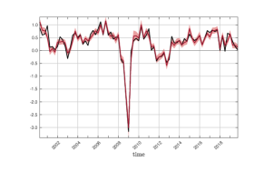
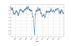
GDP growth rate	GDP growth rate
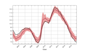
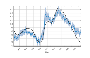
unemployment rate	unemployment rate
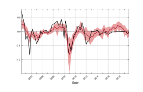
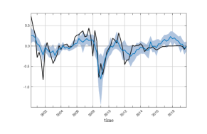
3-months interest rate	3-months interest rate
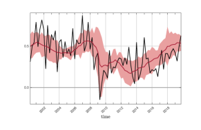
GDP deflator inflation rate	GDP deflator inflation rate
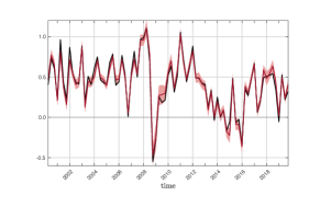
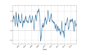
HICP inflation rate	HICP inflation rate

11 Concluding remarks

In this paper, we have shown two main results. First, when estimating an approximate static or dynamic factor model by QML, possibly via the EM algorithm, and using a mis-specified log-likelihood for an exact factor model, the estimated loadings are asymptotically equivalent to the loadings estimated via PC analysis. Why should then we be using the QML estimator rather than the PC estimator of the loadings? The main reason put forward by the literature seems to be the possibility of easily imposing constraints on the loadings, e.g., incorporating prior beliefs.

Second, we have also shown that the factors estimated via WLS or via the Kalman filter/smoother, are all asymptotically equivalent, and these estimators should be always preferred over the PC estimators as they address the heteroskedasticity of the idiosyncratic components so they might even be more efficient (depending on the amount of neglected cross-sectional correlations). Furthermore, in a time series setting the Kalman filter/smoother should be preferred as it allows to easily deal with missing values and given its dynamic aggregation property it can handle very persistent or even non-stationary data without any modification.

Summing up, although the QML plus WLS estimation approach, proposed by Bai and Li (2016), is asymptotically equivalent to the EM plus Kalman smoother approach, proposed by Doz et al. (2012), the latter is likely to produce estimated factors which enjoy better final sample properties and is a more flexible approach for dealing with complex economic datasets. Relevant examples of the use of this estimation technique are: (i) counterfactual analysis (Giannone et al., 2006, 2019); (ii) conditional forecasts (Bańbura et al., 2015); (iii) nowcasting (Giannone et al., 2005, 2008, 2016; Bańbura et al., 2013; Modugno, 2013); (iv) dealing with data irregularly spaced in time (Mariano and Murasawa, 2003; Jungbacker et al., 2011; Bańbura and Modugno, 2014); (v) imposing constraints on the loadings to account for smooth cross-sectional dependence in the case of ordered units (Koopman and van der Wel, 2013; Jungbacker et al., 2014) or for a block-specific factor structure (Coroneo et al., 2016; Altavilla et al., 2017; Delle Chiaie et al., 2021; Barigozzi et al., 2021); (vi) building indicators of the economic activity (Reis and Watson, 2010; Barigozzi and Luciani, 2021; Ng and Scanlan, 2023); (vi) impulse response analysis (Juvenal and Petrella, 2015; Luciani, 2015); (vii) the analysis of stock markets (Linton et al., 2022); (viii) firm-level or household-level repeated cross-sections of data (Barigozzi and Pellegrino, 2023).

Appendix A Kalman filter and Kalman smoother

The following iterations are stated assuming that the true value of the parameters $\bm{\varphi}$ is given and for given initial conditions $\mathbf{F}_{0|0}$ and $\mathbf{P}_{0|0}$.

The Kalman filter is based on the forward iterations for $t=1,\ldots,T$:

$$\mathbf{F}_{t|t-1}=\mathbf{A}\mathbf{F}_{t-1|t-1},$$

$$\mathbf{P}_{t|t-1}=\mathbf{A}\mathbf{P}_{t-1|t-1}\mathbf{A}^{\prime}+\mathbf{H}\mathbf{H}^{\prime},$$

$$\mathbf{F}_{t|t}=\mathbf{F}_{t|t-1}+\mathbf{P}_{t|t-1}\bm{\Lambda}^{\prime}(\bm{\Lambda}\mathbf{P}_{t|t-1}\bm{\Lambda}^{\prime}+\bm{\Sigma}^{\xi})^{-1}(\mathbf{x}_{t}-\bar{\mathbf{x}}-\bm{\Lambda}\mathbf{F}_{t|t-1}),$$

$$\mathbf{P}_{t|t}=\mathbf{P}_{t|t-1}-\mathbf{P}_{t|t-1}\bm{\Lambda}^{\prime}(\bm{\Lambda}\mathbf{P}_{t|t-1}\bm{\Lambda}^{\prime}+\bm{\Sigma}^{\xi})^{-1}\bm{\Lambda}\mathbf{P}_{t|t-1}.$$

Alternatively for $t=1,\ldots,T$ (by Woodbury formula)

$$\mathbf{F}_{t|t}=\mathbf{F}_{t|t-1}+(\bm{\Lambda}^{\prime}(\bm{\Sigma}^{\xi})^{-1}\bm{\Lambda}+\mathbf{P}_{t|t-1}^{-1})^{-1}\bm{\Lambda}^{\prime}(\bm{\Sigma}^{\xi})^{-1}(\mathbf{x}_{t}-\bar{\mathbf{x}}-\bm{\Lambda}\mathbf{F}_{t|t-1}),$$

$$\mathbf{P}_{t|t}=\mathbf{P}_{t|t-1}-(\bm{\Lambda}^{\prime}(\bm{\Sigma}^{\xi})^{-1}\bm{\Lambda}+\mathbf{P}_{t|t-1}^{-1})^{-1}\bm{\Lambda}^{\prime}(\bm{\Sigma}^{\xi})^{-1}\bm{\Lambda}\mathbf{P}_{t|t-1}.$$

The Kalman Smoother is then based on the backward iterations for $t=T,\ldots,1$:

$$\mathbf{F}_{t|T} =\mathbf{F}_{t|t}+\mathbf{P}_{t|t}\mathbf{A}^{\prime}\mathbf{P}_{t+1|t}^{-1}(\mathbf{F}_{t+1|T}-\mathbf{F}_{t+1|t}),$$

$$\mathbf{P}_{t|T} =\mathbf{P}_{t|t}+\mathbf{P}_{t|t}\mathbf{A}^{\prime}\mathbf{P}_{t+1|t}^{-1}(\mathbf{P}_{t+1|T}-\mathbf{P}_{t+1|t})\mathbf{P}_{t+1|t}^{-1}\mathbf{A}\mathbf{P}_{t|t}.$$

Alternatively for $t=T,\ldots,1$ (see, e.g., Durbin and Koopman, 2012, Chapter 4.4, pp.87-91)

$$\mathbf{F}_{t|T}=\mathbf{F}_{t|t-1}+\mathbf{P}_{t|t-1}\mathbf{r}_{t-1},$$

$$\mathbf{r}_{t-1}=\bm{\Lambda}^{\prime}(\bm{\Lambda}\mathbf{P}_{t|t-1}\bm{\Lambda}^{\prime}+\bm{\Sigma}^{\xi})^{-1}(\mathbf{x}_{t}-\bar{\mathbf{x}}-\bm{\Lambda}\mathbf{F}_{t|t-1})+\mathbf{L}^{\prime}_{t}\mathbf{r}_{t},$$

$$\mathbf{P}_{t|T}=\mathbf{P}_{t|t-1}(\mathbf{I}_{r}-\mathbf{N}_{t-1}\mathbf{P}_{t|t-1}),$$

$$\mathbf{N}_{t-1}=\bm{\Lambda}_{n}^{\prime}(\bm{\Lambda}\mathbf{P}_{t|t-1}\bm{\Lambda}^{\prime}+\bm{\Sigma}^{\xi})^{-1}\bm{\Lambda}+\mathbf{L}_{t}^{\prime}\mathbf{N}_{t}\mathbf{L}_{t},$$

$$\mathbf{L}_{t}=\mathbf{A}-\mathbf{A}\mathbf{P}_{t|t-1}\bm{\Lambda}^{\prime}(\bm{\Lambda}\mathbf{P}_{t|t-1}\bm{\Lambda}^{\prime}+\bm{\Sigma}^{\xi})^{-1}\bm{\Lambda},$$

$$\mathbf{C}_{t,t+1|T}=\mathbf{P}_{t|t-1}\mathbf{L}_{t}^{\prime}(\mathbf{I}_{r}-\mathbf{N}_{t}\mathbf{P}_{t+1|t}),\qquad\mathbf{C}_{t,t-1|T}=\mathbf{C}_{t,t+1|T}^{\prime},$$

where $\mathbf{r}_{T}=\mathbf{0}_{r}$, $\mathbf{N}_{T}=\mathbf{0}_{r}$.

Appendix B Joint distribution of $\boldsymbol{\mathcal{X}}$ and $\boldsymbol{\mathcal{F}}$

First, notice that, by Assumptions 6(a) and 6(g), for any $t=1,\ldots,T$, $\mathbf{F}_{t}=\sum_{k=0}^{t-1}\mathbf{A}^{k}\mathbf{H}\mathbf{u}_{t-k}$, which, under Assumption 8(b), is a linear combination of $t$ jointly Gaussians. Therefore, for all $T\in\mathbb{N}$,

$$\bm{\mathcal{F}}\sim\mathcal{N}(\mathbf{0}_{rT},\bm{\Omega}^{F}).$$ (76)

Moreover, by Assumption 8(a) and (76), and since $\bm{\mathcal{Z}}$ and $\bm{\mathcal{F}}$ are independent by Assumption 3, the joint density of $\bm{\mathcal{Z}}$ and $\bm{\mathcal{F}}$ is such that, for all $N,T\in\mathbb{N}$:

$$f (\bm{\mathcal{Z}},\bm{\mathcal{F}})=f(\bm{\mathcal{Z}})f(\bm{\mathcal{F}})$$

$$=\frac{1}{(2\pi)^{NT}\sqrt{\det(\bm{\Omega}^{\xi})}}\exp\left\{-\frac{1}{2}\bm{\mathcal{Z}}^{\prime}(\bm{\Omega}^{\xi})^{-1}\bm{\mathcal{Z}}\right\}\frac{1}{(2\pi)^{rT}\sqrt{\det(\bm{\Omega}^{F})}}\exp\left\{-\frac{1}{2}\bm{\mathcal{F}}^{\prime}(\bm{\Omega}^{F})^{-1}\bm{\mathcal{F}}\right\}$$ (77)

$$=\frac{1}{(2\pi)^{(N+r)T}\sqrt{\det(\bm{\Omega}^{\xi})\det(\bm{\Omega}^{F})}}\exp\left\{-\frac{1}{2}\left(\begin{array}[]{c}\bm{\mathcal{Z}}\\ \bm{\mathcal{F}}\end{array}\right)^{\prime}\left(\begin{array}[]{cc}\bm{\Omega}^{\xi}&\mathbf{0}_{NT\times rT}\\ \mathbf{0}_{rT\times NT}&\bm{\Omega}^{F}\end{array}\right)^{-1}\left(\begin{array}[]{c}\bm{\mathcal{Z}}\\ \bm{\mathcal{F}}\end{array}\right)\right\}$$ (84)

$$=\frac{1}{(2\pi)^{(N+r)T}\sqrt{\det(\bm{\Omega}^{\xi})\det(\bm{\Omega}^{F})}}\exp\left\{-\frac{1}{2}\left(\begin{array}[]{c}\bm{\mathcal{X}}-\bm{\mathcal{A}}-\bm{\mathfrak{L}}\bm{\mathcal{F}}\\ \bm{\mathcal{F}}\end{array}\right)^{\prime}\left(\begin{array}[]{cc}\bm{\Omega}^{\xi}&\mathbf{0}_{NT\times rT}\\ \mathbf{0}_{rT\times NT}&\bm{\Omega}^{F}\end{array}\right)^{-1}\left(\begin{array}[]{c}\bm{\mathcal{X}}-\bm{\mathcal{A}}-\bm{\mathfrak{L}}\bm{\mathcal{F}}\\ \bm{\mathcal{F}}\end{array}\right)\right\},$$ (91)

which is equivalent to saying:

$$\left(\begin{array}[]{c}\bm{\mathcal{Z}}\\ \bm{\mathcal{F}}\end{array}\right)\sim\mathcal{N}\left(\left(\begin{array}[]{c}\mathbf{0}_{NT}\\ \mathbf{0}_{rT}\end{array}\right),\left(\begin{array}[]{cc}\bm{\Omega}^{\xi}&\mathbf{0}_{NT\times rT}\\ \mathbf{0}_{rT\times NT}&\bm{\Omega}^{F}\end{array}\right)\right).$$ (92)

Clearly, we have $\mathbb{E}[\bm{\mathcal{X}}|\bm{\mathcal{F}}]=\bm{\mathcal{A}}+\bm{\mathfrak{L}}\bm{\mathcal{F}}+\mathbb{E}[\bm{\mathcal{Z}}|\bm{\mathcal{F}}]=\bm{\mathcal{A}}+\bm{\mathfrak{L}}\bm{\mathcal{F}}+\mathbb{E}[\bm{\mathcal{Z}}]=\bm{\mathcal{A}}+\bm{\mathfrak{L}}\bm{\mathcal{F}}$, by Assumption 3, and $\mathbb{C}\text{ov}(\bm{\mathcal{X}}|\bm{\mathcal{F}})=\bm{\Omega}^{\xi}$. Thus, from the last line of (77) we see that $f(\bm{\mathcal{X}}|\bm{\mathcal{F}})=f(\bm{\mathcal{Z}})$. It follows that the joint density of $\bm{\mathcal{X}}$ and $\bm{\mathcal{F}}$ is such that:

$$f(\bm{\mathcal{X}},\bm{\mathcal{F}})=f(\bm{\mathcal{X}}|\bm{\mathcal{F}})f(\bm{\mathcal{F}})=f(\bm{\mathcal{Z}})f(\bm{\mathcal{F}})=f(\bm{\mathcal{Z}},\bm{\mathcal{F}}),$$ (93)

and the right-hand side is Gaussian because of (92). To verify (93) directly, notice that the distribution given in (35) is is equivalent to (92). Indeed, on the one hand, from the last line of (77) we have:

$$f(\bm{\mathcal{Z}},\bm{\mathcal{F}})=\frac{1}{(2\pi)^{(N+r)T}\sqrt{\det(\bm{\Omega}^{\xi})\det(\bm{\Omega}^{F})}}\exp\Bigg{\{}-\frac{1}{2}\bigg{[} (\bm{\mathcal{X}}-\bm{\mathcal{A}})^{\prime}(\bm{\Omega}^{\xi})^{-1}(\bm{\mathcal{X}}-\bm{\mathcal{A}})-(\bm{\mathcal{X}}-\bm{\mathcal{A}})^{\prime}(\bm{\Omega}^{\xi})^{-1}\bm{\mathfrak{L}}\bm{\mathcal{F}}$$

$$-\bm{\mathcal{F}}^{\prime}\bm{\mathfrak{L}}^{\prime}(\bm{\Omega}^{\xi})^{-1}(\bm{\mathcal{X}}-\bm{\mathcal{A}})+\bm{\mathcal{F}}^{\prime}\bm{\mathfrak{L}}^{\prime}(\bm{\Omega}^{\xi})^{-1}\bm{\mathfrak{L}}\bm{\mathcal{F}}+\bm{\mathcal{F}}^{\prime}(\bm{\Omega}^{F})^{-1}\bm{\mathcal{F}}\bigg{]}\Bigg{\}},$$

On the other hand, letting $\bm{\mathfrak{P}}:=\left((\bm{\Omega}^{F})^{-1}+\bm{\mathfrak{L}}^{\prime}(\bm{\Omega}^{\xi})^{-1}\bm{\mathfrak{L}}\right)$, from (35) we have

$$f(\bm{\mathcal{X}},\bm{\mathcal{F}})=\frac{1}{(2\pi)^{(N+r)T}\sqrt{\det\left(\begin{array}[]{cc}\bm{\Omega}^{x}&\bm{\mathfrak{L}}\bm{\Omega}^{F}\\ \bm{\Omega}^{F}\bm{\mathfrak{L}}^{\prime}&\bm{\Omega}^{F}\end{array}\right)}}\exp\Bigg{\{}-\frac{1}{2}\;\; \left(\begin{array}[]{c}\bm{\mathcal{X}}-\bm{\mathcal{A}}\\ \bm{\mathcal{F}}\end{array}\right)^{\prime}\left(\begin{array}[]{cc}\bm{\Omega}^{x}&\bm{\mathfrak{L}}\bm{\Omega}^{F}\\ \bm{\Omega}^{F}\bm{\mathfrak{L}}^{\prime}&\bm{\Omega}^{F}\end{array}\right)^{-1}\left(\begin{array}[]{c}\bm{\mathcal{X}}-\bm{\mathcal{A}}\\ \bm{\mathcal{F}}\end{array}\right)\Bigg{\}}$$ (102)

$$=\frac{1}{(2\pi)^{(N+r)T}\sqrt{\det(\bm{\Omega}^{\xi})\det(\bm{\Omega}^{F})}}\exp\Bigg{\{}-\frac{1}{2}\bigg{[} (\bm{\mathcal{X}}-\bm{\mathcal{A}})^{\prime}(\bm{\Omega}^{\xi})^{-1}(\bm{\mathcal{X}}-\bm{\mathcal{A}})-(\bm{\mathcal{X}}-\bm{\mathcal{A}})^{\prime}(\bm{\Omega}^{\xi})^{-1}\bm{\mathfrak{L}}\bm{\mathcal{F}}$$

$$-\bm{\mathcal{F}}^{\prime}\left(\bm{\Omega}^{F}-\bm{\Omega}^{F}\bm{\mathfrak{L}}^{\prime}(\bm{\Omega}^{x})^{-1}\bm{\mathfrak{L}}\bm{\Omega}^{F}\right)^{-1}\bm{\Omega}^{F}\bm{\mathfrak{L}}^{\prime}(\bm{\Omega}^{x})^{-1}(\bm{\mathcal{X}}-\bm{\mathcal{A}})$$

$$+\bm{\mathcal{F}}^{\prime}\left(\bm{\Omega}^{F}-\bm{\Omega}^{F}\bm{\mathfrak{L}}^{\prime}(\bm{\Omega}^{x})^{-1}\bm{\mathfrak{L}}\bm{\Omega}^{F}\right)^{-1}\bm{\mathcal{F}}\bigg{]}\Bigg{\}}$$

$$=\frac{1}{(2\pi)^{(N+r)T}\sqrt{\det(\bm{\Omega}^{\xi})\det(\bm{\Omega}^{F})}}\exp\Bigg{\{}-\frac{1}{2}\bigg{[} (\bm{\mathcal{X}}-\bm{\mathcal{A}})^{\prime}(\bm{\Omega}^{\xi})^{-1}(\bm{\mathcal{X}}-\bm{\mathcal{A}})-(\bm{\mathcal{X}}-\bm{\mathcal{A}})^{\prime}(\bm{\Omega}^{\xi})^{-1}\bm{\mathfrak{L}}\bm{\mathcal{F}}$$

$$-\bm{\mathcal{F}}^{\prime}\bm{\mathfrak{P}}\bm{\mathfrak{P}}^{-1}\bm{\mathfrak{L}}^{\prime}(\bm{\Omega}^{\xi})^{-1}(\bm{\mathcal{X}}-\bm{\mathcal{A}})+\bm{\mathcal{F}}^{\prime}\bm{\mathfrak{P}}\bm{\mathcal{F}}\bigg{]}\Bigg{\}}$$

$$=\frac{1}{(2\pi)^{(N+r)T}\sqrt{\det(\bm{\Omega}^{\xi})\det(\bm{\Omega}^{F})}}\exp\Bigg{\{}-\frac{1}{2}\bigg{[} (\bm{\mathcal{X}}-\bm{\mathcal{A}})^{\prime}(\bm{\Omega}^{\xi})^{-1}(\bm{\mathcal{X}}-\bm{\mathcal{A}})-(\bm{\mathcal{X}}-\bm{\mathcal{A}})^{\prime}(\bm{\Omega}^{\xi})^{-1}\bm{\mathfrak{L}}\bm{\mathcal{F}}$$

$$-\bm{\mathcal{F}}^{\prime}\bm{\mathfrak{L}}^{\prime}(\bm{\Omega}^{\xi})^{-1}(\bm{\mathcal{X}}-\bm{\mathcal{A}})+\bm{\mathcal{F}}^{\prime}\bm{\mathfrak{L}}^{\prime}(\bm{\Omega}^{\xi})^{-1}\bm{\mathfrak{L}}\bm{\mathcal{F}}+\bm{\mathcal{F}}^{\prime}(\bm{\Omega}^{F})^{-1}\bm{\mathcal{F}}\bigg{]}\Bigg{\}}$$

$$=f(\bm{\mathcal{Z}},\bm{\mathcal{F}}).\qquad\qquad\qquad\qquad\qquad\qquad\qquad\;\;\;$$ (103)

To derive (103) we used the formula of the determinant of a block matrix:

$$\det\left(\begin{array}[]{cc}\bm{\Omega}^{x}&\bm{\mathfrak{L}}\bm{\Omega}^{F}\\ \bm{\Omega}^{F}\bm{\mathfrak{L}}^{\prime}&\bm{\Omega}^{F}\end{array}\right)=\det\left(\bm{\Omega}^{x}-\bm{\mathfrak{L}}\bm{\Omega}^{F}(\bm{\Omega}^{F})^{-1}\bm{\Omega}^{F}\bm{\mathfrak{L}}^{\prime}\right)\det(\bm{\Omega}^{F})=\det(\bm{\Omega}^{\xi})\det(\bm{\Omega}^{F});$$

the formula for inversion of a block-matrix:

$$\left(\begin{array}[]{cc}\bm{\Omega}^{x}&\bm{\mathfrak{L}}\bm{\Omega}^{F}\\ \bm{\Omega}^{F}\bm{\mathfrak{L}}^{\prime}&\bm{\Omega}^{F}\end{array}\right)^{-1}$$ (106)

$$=\left(\begin{array}[]{cc}\left(\bm{\Omega}^{x}-\bm{\mathfrak{L}}\bm{\Omega}^{F}(\bm{\Omega}^{F})^{-1}\bm{\Omega}^{F}\bm{\mathfrak{L}}^{\prime}\right)^{-1}&\mathbf{0}_{NT\times rT}\\ \mathbf{0}_{rT\times NT}&\left(\bm{\Omega}^{F}-\bm{\Omega}^{F}\bm{\mathfrak{L}}^{\prime}(\bm{\Omega}^{x})^{-1}\bm{\mathfrak{L}}\bm{\Omega}^{F}\right)^{-1}\end{array}\right)\left(\begin{array}[]{cc}\mathbf{I}_{NT}&-\bm{\mathfrak{L}}\bm{\Omega}^{F}(\bm{\Omega}^{F})^{-1}\\ -\bm{\Omega}^{F}\bm{\mathfrak{L}}^{\prime}(\bm{\Omega}^{x})^{-1}&\mathbf{I}_{rT}\end{array}\right)$$ (111)

$$=\left(\begin{array}[]{cc}(\bm{\Omega}^{\xi})^{-1}&\mathbf{0}_{NT\times rT}\\ \mathbf{0}_{rT\times NT}&\left(\bm{\Omega}^{F}-\bm{\Omega}^{F}\bm{\mathfrak{L}}^{\prime}(\bm{\Omega}^{x})^{-1}\bm{\mathfrak{L}}\bm{\Omega}^{F}\right)^{-1}\end{array}\right)\left(\begin{array}[]{cc}\mathbf{I}_{NT}&-\bm{\mathfrak{L}}\\ -\bm{\Omega}^{F}\bm{\mathfrak{L}}^{\prime}(\bm{\Omega}^{x})^{-1}&\mathbf{I}_{rT}\end{array}\right)$$ (116)

$$=\left(\begin{array}[]{cc}(\bm{\Omega}^{\xi})^{-1}&-(\bm{\Omega}^{\xi})^{-1}\bm{\mathfrak{L}}\\ -\left(\bm{\Omega}^{F}-\bm{\Omega}^{F}\bm{\mathfrak{L}}^{\prime}(\bm{\Omega}^{x})^{-1}\bm{\mathfrak{L}}\bm{\Omega}^{F}\right)^{-1}\bm{\Omega}^{F}\bm{\mathfrak{L}}^{\prime}(\bm{\Omega}^{x})^{-1}&\left(\bm{\Omega}^{F}-\bm{\Omega}^{F}\bm{\mathfrak{L}}^{\prime}(\bm{\Omega}^{x})^{-1}\bm{\mathfrak{L}}\bm{\Omega}^{F}\right)^{-1}\end{array}\right);$$ (119)

and the Woodbury identities:

$$\left(\bm{\Omega}^{F}-\bm{\Omega}^{F}\bm{\mathfrak{L}}^{\prime}(\bm{\Omega}^{x})^{-1}\bm{\mathfrak{L}}\bm{\Omega}^{F}\right)^{-1}=\left(\bm{\Omega}^{F}-\bm{\Omega}^{F}\bm{\mathfrak{L}}^{\prime}\left(\bm{\mathfrak{L}}\bm{\Omega}^{F}\bm{\mathfrak{L}}^{\prime}+\bm{\Omega}^{\xi}\right)^{-1}\bm{\mathfrak{L}}\bm{\Omega}^{F}\right)^{-1}=(\bm{\Omega}^{F})^{-1}+\bm{\mathfrak{L}}^{\prime}(\bm{\Omega}^{\xi})^{-1}\bm{\mathfrak{L}}=\bm{\mathfrak{P}},$$

$$\bm{\Omega}^{F}\bm{\mathfrak{L}}^{\prime}(\bm{\Omega}^{x})^{-1}=\bm{\Omega}^{F}\bm{\mathfrak{L}}^{\prime}\left(\bm{\mathfrak{L}}\bm{\Omega}^{F}\bm{\mathfrak{L}}^{\prime}+\bm{\Omega}^{\xi}\right)^{-1}=\left((\bm{\Omega}^{F})^{-1}+\bm{\mathfrak{L}}^{\prime}(\bm{\Omega}^{\xi})^{-1}\bm{\mathfrak{L}}\right)^{-1}\bm{\mathfrak{L}}^{\prime}(\bm{\Omega}^{\xi})^{-1}=\bm{\mathfrak{P}}^{-1}\bm{\mathfrak{L}}^{\prime}(\bm{\Omega}^{\xi})^{-1}.$$

Appendix C Identification of simulated factors and loadings

Let $\bm{L}:=(\bm{\ell}_{1}\cdots\bm{\ell}_{N})^{\prime}$ and define:

$$\widetilde{\bm{R}}:=\left(\bm{L}^{\prime}\widetilde{\mathbf{V}}^{\chi}\widetilde{\mathbf{V}}^{\chi\prime}\bm{L}\right)^{-1}\bm{L}^{\prime}\widetilde{\mathbf{V}}^{\chi}\widetilde{\bm{\mathcal{S}}}(\widetilde{\mathbf{M}}^{\chi})^{1/2},$$

First, notice that $\widetilde{\bm{\Gamma}}^{\chi}$ is a consistent estimator of ${\bm{\Gamma}}^{\chi}$ and so the eigenvectors and eigenvalues of $\widetilde{\bm{\Gamma}}^{\chi}$ are consistent estimators of the eigenvectors and eigenvalues of ${\bm{\Gamma}}^{\chi}$. Therefore, with probability tending to one as $N,T\to\infty$, $N^{-1}\widetilde{\mathbf{M}}^{\chi}$ is finite and invertible and the columns of $\bm{L}$ and of $\widetilde{\mathbf{V}}^{\chi}$ span the same space, thus

$$\bm{L}\left(\bm{L}^{\prime}\bm{L}\right)^{-1}\bm{L}^{\prime}\widetilde{\mathbf{V}}^{\chi}=\widetilde{\mathbf{V}}^{\chi},$$ (120)

$$\widetilde{\mathbf{V}}^{\chi}\left(\widetilde{\mathbf{V}}^{\chi\prime}\widetilde{\mathbf{V}}^{\chi}\right)^{-1}\widetilde{\mathbf{V}}^{\chi\prime}\bm{L}=\widetilde{\mathbf{V}}^{\chi}\widetilde{\mathbf{V}}^{\chi\prime}\bm{L}=\bm{L},$$ (121)

$$\text{rk}\left(\bm{L}^{\prime}\widetilde{\mathbf{V}}^{\chi}\right)=r.$$ (122)

It follows that $\bm{L}^{\prime}\widetilde{\mathbf{V}}^{\chi}$ is invertible, and $(\bm{L}^{\prime}\widetilde{\mathbf{V}}^{\chi}\widetilde{\mathbf{V}}^{\chi\prime}\bm{L})^{-1}=(\bm{L}^{\prime}\bm{L})^{-1}$ is well defined. Therefore, $\widetilde{\bm{R}}=O_{\mathrm{P}}(1)$ and $(\widetilde{\bm{R}})^{-1}=O_{\mathrm{P}}(1)$.

Finally, by (120), (121), and (122)

$$\bm{L}\widetilde{\bm{R}}=\bm{L}\left(\bm{L}^{\prime}\widetilde{\mathbf{V}}^{\chi}\widetilde{\mathbf{V}}^{\chi\prime}\bm{L}\right)^{-1}\bm{L}^{\prime}\widetilde{\mathbf{V}}^{\chi}\widetilde{\bm{\mathcal{S}}}(\widetilde{\mathbf{M}}^{\chi})^{1/2}=\bm{L}\left(\bm{L}^{\prime}\bm{L}\right)^{-1}\bm{L}^{\prime}\widetilde{\mathbf{V}}^{\chi}\widetilde{\bm{\mathcal{S}}}(\widetilde{\mathbf{M}}^{\chi})^{1/2}=\widetilde{\mathbf{V}}^{\chi}\widetilde{\bm{\mathcal{S}}}(\widetilde{\mathbf{M}}^{\chi})^{1/2}=\bm{\Lambda},$$

$$\widetilde{\bm{R}}^{-1}\bm{f}_{t}=(\widetilde{\mathbf{M}}^{\chi})^{-1/2}\widetilde{\bm{\mathcal{S}}}\left(\bm{L}^{\prime}\widetilde{\mathbf{V}}^{\chi}\right)^{-1}\bm{L}^{\prime}\widetilde{\mathbf{V}}^{\chi}\widetilde{\mathbf{V}}^{\chi\prime}\bm{L}\bm{f}_{t}=(\widetilde{\mathbf{M}}^{\chi})^{-1/2}\widetilde{\bm{\mathcal{S}}}\widetilde{\mathbf{V}}^{\chi\prime}\bm{L}\bm{f}_{t}=(\widetilde{\mathbf{M}}^{\chi})^{-1/2}\widetilde{\bm{\mathcal{S}}}\widetilde{\mathbf{V}}^{\chi\prime}\bm{\chi}_{t}=\mathbf{F}_{t}.$$

References

- Ahn and Horenstein (2013) Ahn, S. C. and A. R. Horenstein (2013). Eigenvalue ratio test for the number of factors. Econometrica 81, 1203–1227.
- Aït-Sahalia and Xiu (2017) Aït-Sahalia, Y. and D. Xiu (2017). Using principal component analysis to estimate a high dimensional factor model with high-frequency data. Journal of Econometrics 201, 384–399.
- Alessi et al. (2010) Alessi, L., M. Barigozzi, and M. Capasso (2010). Improved penalization for determining the number of factors in approximate static factor models. Statistics and Probability Letters 80, 1806–1813.
- Altavilla et al. (2017) Altavilla, C., R. Giacomini, and G. Ragusa (2017). Anchoring the yield curve using survey expectations. Journal of Applied Econometrics 32, 1055–1068.
- Amemiya et al. (1987) Amemiya, Y., W. A. Fuller, and S. G. Pantula (1987). The asymptotic distributions of some estimators for a factor analysis model. Journal of Multivariate Analysis 22, 51–64.
- Anderson and Deistler (2008) Anderson, B. D. O. and M. Deistler (2008). Generalized linear dynamic factor models-A structure theory. In Proceedings of the 47th IEEE Conference on Decision and Control, pp. 1980–1985.
- Anderson and Moore (1979) Anderson, B. D. O. and J. B. Moore (1979). Optimal Filtering. Dover Publications, Inc.
- Anderson (2003) Anderson, T. W. (2003). An Inrtoduction to Multivariate Statistical Analysis. Wiley series in Probability and Mathematical Statistics.
- Anderson and Amemiya (1988) Anderson, T. W. and Y. Amemiya (1988). The asymptotic normal distribution of estimators in factor analysis under general conditions. The Annals of Statistics 16, 759–771.
- Anderson and Rubin (1956) Anderson, T. W. and H. Rubin (1956). Statistical inference in factor analysis. In Proceedings of the third Berkeley symposium on mathematical statistics and probability, Volume 5, pp. 111–150.
- Andrews (1991) Andrews, D. W. (1991). Heteroskedasticity and autocorrelation consistent covariance matrix estimation. Econometrica 59, 817–858.
- Austern and Orbanz (2022) Austern, M. and P. Orbanz (2022). Limit theorems for distributions invariant under groups of transformations. The Annals of Statistics 50, 1960–1991.
- Bai (2003) Bai, J. (2003). Inferential theory for factor models of large dimensions. Econometrica 71, 135–171.
- Bai and Li (2012) Bai, J. and K. Li (2012). Statistical analysis of factor models of high dimension. The Annals of Statistics 40, 436–465.
- Bai and Li (2016) Bai, J. and K. Li (2016). Maximum likelihood estimation and inference for approximate factor models of high dimension. The Review of Economics and Statistics 98, 298–309.
- Bai and Liao (2016) Bai, J. and Y. Liao (2016). Efficient estimation of approximate factor models via penalized maximum likelihood. Journal of Econometrics 191, 1–18.
- Bai and Ng (2002) Bai, J. and S. Ng (2002). Determining the number of factors in approximate factor models. Econometrica 70, 191–221.
- Bai and Ng (2006) Bai, J. and S. Ng (2006). Confidence intervals for diffusion index forecasts and inference for factor augmented regressions. Econometrica 74, 1133–1150.
- Bai and Ng (2013) Bai, J. and S. Ng (2013). Principal components estimation and identification of static factors. Journal of Econometrics 176, 18–29.
- Bai and Ng (2020) Bai, J. and S. Ng (2020). Simpler proofs for approximate factor models of large dimensions. Technical Report arXiv:2008.00254.
- Bai and Ng (2021) Bai, J. and S. Ng (2021). Approximate factor models with weaker loadings. Technical Report arXiv:2109.03773.
- Bańbura et al. (2015) Bańbura, M., D. Giannone, and M. Lenza (2015). Conditional forecasts and scenario analysis with vector autoregressions for large cross-sections. International Journal of Forecasting 31, 739–756.
- Bańbura et al. (2013) Bańbura, M., D. Giannone, M. Modugno, and L. Reichlin (2013). Now-casting and the real-time data flow. In Handbook of economic forecasting, Volume 2, pp. 195–237. Elsevier.
- Bańbura and Modugno (2014) Bańbura, M. and M. Modugno (2014). Maximum likelihood estimation of factor models on datasets with arbitrary pattern of missing data. Journal of Applied Econometrics 29, 133–160.
- Barigozzi (2022) Barigozzi, M. (2022). On estimation and inference of large approximate dynamic factor models via the principal component analysis. Technical report. arXiv:2211.01921.v3.
- Barigozzi (2023) Barigozzi, M. (2023). Asymptotic equivalence of principal component and quasi maximum likelihood estimators in large approximate factor models. Technical report. arXiv:2307.09864.v2.
- Barigozzi et al. (2014) Barigozzi, M., A. M. Conti, and M. Luciani (2014). Do euro area countries respond asymmetrically to the common monetary policy? Oxford Bulletin of Economics and Statistics 76, 693–714.
- Barigozzi et al. (2021) Barigozzi, M., A. Cuzzola, M. Grazzi, and D. Moschella (2021). Factoring in the micro: A transaction-level dynamic factor approach to the decomposition of export volatility. LEM working papers 2021/22, Institute of Economics Sant’Anna School of Advanced Studies.
- Barigozzi and Hallin (2020) Barigozzi, M. and M. Hallin (2020). Generalized dynamic factor models and volatilities: Consistency, rates, and prediction intervals. Journal of Econometrics 216, 4–34.
- Barigozzi and Hallin (2024) Barigozzi, M. and M. Hallin (2024). Dynamic factor models: A genealogy. In N. Ngoc Thach, N. D. Trung, D. T. Ha, and K. V. (Eds.), Partial Identification in Econometrics and Related Topics. Studies in Systems, Decision and Control. Springer.
- Barigozzi et al. (2021) Barigozzi, M., M. Lippi, and M. Luciani (2021). Large-dimensional dynamic factor models: Estimation of impulse-response functions with cointegrated factors. Journal of Econometrics 221, 455–482.
- Barigozzi and Lissona (2024) Barigozzi, M. and C. Lissona (2024). The euro area output gap. Technical report. mimeo.