The physics of gravitational waves

Abstract

These lecture notes collect the material that I have been using over the years for various short courses on the physics of gravitational waves, first at the Institut d’Astrophysique de Paris (France), and then at SISSA (Italy) and various summer/winter schools. The level should be appropriate for PhD students in physics or for MSc students that have taken a first course in general relativity. I try as much as possible to derive results from first principles and focus on the physics, rather than on astrophysical applications. The reason is not only that the latter require a solid understanding of the physics, but it also lies in the trove of data that are being uncovered by the LIGO-Virgo-KAGRA collaboration after the first direct detection of gravitational waves GW150914 . Any attempt to summarize such a rich and fast changing landscape and its evolving astrophysical interpretation is bound to become obsolete before the ink hits the page.

I Prerequisites

These notes assume familiarity with Einstein’s equations, which in units with $G=c=1$ can be written as

$$G_{\mu\nu}=8\pi T_{\mu\nu}\,,$$ (1)

with $G^{\mu\nu}$ the Einstein tensor and $T^{\mu\nu}$ the matter stress energy tensor. It may be useful to recall that because of the Bianchi identity $\nabla_{\mu}G^{\mu\nu}=0$, the stress energy tensor satisfies the “conservation” equation $\nabla_{\mu}T^{\mu\nu}=0$ on shell.

For a perfect fluid, in the $(-+++)$ signature that we will use throughout these notes, the stress energy tensor takes the form

$$T^{\mu\nu}=(\rho+p)u^{\mu}u^{\nu}+pg^{\mu\nu},$$ (2)

where $u^{\mu}$ is the 4-velocity of the fluid element, $\rho$ the energy density and $p$ the pressure. With this ansatz, the conservation of the stress energy tensor implies

$$\frac{\mathrm{d\rho}}{\mathrm{d}\tau}=-(p+\rho)\nabla_{\mu}u^{\mu}\,,$$ (3)

with $\tau$ the fluid element’s proper time, and

$$a^{\mu}=-\frac{\gamma^{\mu\nu}\partial_{\nu}p}{\rho+p}\,,$$ (4)

with $a^{\mu}=u^{\nu}\nabla_{\nu}u^{\mu}$ the 4-acceleration and

$$\gamma^{\mu\nu}=g^{\mu\nu}+u^{\mu}u^{\nu}$$ (5)

the projector on the hypersurface orthogonal to $u^{\mu}$. Let us recall that Eq. (3) simply encodes the conservation of energy, while Eq. (4) generalizes the Newtonian Euler equation. In particular, for $p=0$ the relativistic Euler equation reduces to the geodesic equation $a^{\mu}=0$.

It is worth recalling that the stress energy tensor can be defined in terms of the functional derivative of the matter action, i.e.

$$T^{\mu\nu}=\frac{2}{\sqrt{-g}}\frac{\delta S_{\mathrm{pp}}}{\delta g_{\mu\nu}}.$$ (6)

For a point particle of mass $m$, the action is simply given by

$$S_{\mathrm{pp}}=-m\int\mathrm{d}\tau\,,$$ (7)

where the integral is along the trajectory. By varying this action with respect to the trajectory, one obtains the geodesic equation $a^{\mu}=0$, while the functional derivative with respect to the metric yields

$$T^{\mu\nu}_{\mathrm{pp}}=\frac{m}{\sqrt{-g}}\delta^{(3)}\left(\vec{x}-\vec{X}(t)\right)\frac{u^{\mu}u^{\nu}}{u^{t}}\,,$$ (8)

with $\vec{X}(t)$ the trajectory. This stress energy tensor can be mapped into that of a perfect fluid with $p=0$ (dust). The same clearly applies to a collection of point particles. We can therefore conclude that for point particles, the geodesic equation is implied by the conservation of the stress energy tensor.

Finally, let us recall that the “divergence” or “focusing” of neighboring geodesics is described by the geodesic deviation equation. More precisely, given a family of geodesics $x^{\mu}(v,\tau)$ labeled by a parameter $v$ and the proper time $\tau$, let us introduce the separation vector $v^{\mu}=(\partial x^{\mu}/\partial v)\delta v$ joining two neighboring geodesics with parameters $v$ and $v+\delta v$. This vector then satisfies the geodesic deviation equation

$$\frac{\mathrm{D}^{2}v^{\mu}}{\mathrm{d}\tau^{2}}=R^{\mu}_{\alpha\beta\gamma}u^{\alpha}u^{\beta}v^{\gamma}\,,$$ (9)

with $R^{\mu}_{\alpha\beta\gamma}$ the Riemann tensor and $\mathrm{D}/\mathrm{d}\tau$ the covariant derivative along the four velocity.

Exercise 1: From the action of a point particle, $S=-m\int d\tau$, derive the geodesics equations by varying with respect to the trajectory, and the stress energy tensor by varying with respect to the metric.

II The propagation and generation of gravitational waves

II.1 Linear perturbations on flat space

Let us start by considering generic vacuum perturbations $h_{\mu\nu}$ of a flat background spacetime. The perturbed spacetime’s metric at linear order is therefore given by

$$g_{\mu\nu}=\eta_{\mu\nu}+h_{\mu\nu}\,,\qquad g^{\mu\nu}=\eta^{\mu\nu}-h^{\mu\nu}\,,$$ (10)

where indices are meant to be raised and lowered with the Minkowski metric $\eta_{\mu\nu}$. We will now derive the (linearized) Einstein equations for the metric perturbation $h_{\mu\nu}$.

Let us first recall that the gauge group of GR is given by diffeomorphisms, i.e. coordinate transformations. Under a transformation $\tilde{x}^{\mu}=\tilde{x}^{\mu}(x)$, the metric transforms as

$$\tilde{g}_{\mu\nu}\left(\tilde{x}(x)\right)=\frac{\partial x^{\alpha}}{\partial\tilde{x}^{\mu}}\frac{\partial x^{\beta}}{\partial\tilde{x}^{\nu}}g_{\alpha\beta}(x)\,.$$ (11)

If the coordinate transformation is “infinitesimal”, $\tilde{x}^{\mu}=x^{\mu}+\xi^{\mu}$ with $\partial_{\nu}\xi^{\mu}\ll 1$, a Taylor expansion of Eq. (11) implies that the metric perturbation transforms as

$$\tilde{h}_{\mu\nu}=h_{\mu\nu}-\mathcal{L}_{\xi}\eta_{\mu\nu}=h_{\mu\nu}-\partial_{\mu}\xi_{\nu}-\partial_{\nu}\xi_{\mu}.$$ (12)

where $\mathcal{L}_{\xi}$ is the Lie derivative along the vector field $\xi$.

Let us use this gauge freedom to impose the Lorenz gauge condition

$$\partial_{\mu}\bar{h}^{\mu\nu}=0\,,$$ (13)

where we have introduced the trace-reversed metric perturbation $\bar{h}_{\mu\nu}=h_{\mu\nu}-\frac{1}{2}h\eta_{\mu\nu}$, with $h=\eta_{\mu\nu}h^{\mu\nu}$ the trace. Note that this condition is also known as de Donder gauge condition, or also as harmonic gauge condition (as it can be easily proven that it is equivalent to $\Box x^{\nu}=0$, where $\Box=\eta^{\mu\nu}\partial_{\mu}\partial_{\nu}$ is the flat space d’Alembertian and the $x^{\nu}$ are scalar functions defining the coordinates). In this gauge, it is straightforward to show that the linearized Ricci tensor is

$$R_{\mu\nu}=-\frac{1}{2}\Box h_{\mu\nu}\,.$$ (14)

The Einstein equations can be written in the two equivalent forms

$$R_{\mu\nu}-\frac{1}{2}Rg_{\mu\nu}=8\pi T_{\mu\nu}\quad\Leftrightarrow\quad R_{\mu\nu}=8\pi\left(T_{\mu\nu}-\frac{1}{2}Tg_{\mu\nu}\right).$$ (15)

From the second expression, the linearized equations can therefore be written as

$$\Box h_{\mu\nu}=-16\pi\left(T_{\mu\nu}-\frac{1}{2}Tg_{\mu\nu}\right)\quad\Leftrightarrow\quad\Box\bar{h}_{\mu\nu}=-16\pi T_{\mu\nu}\,,$$ (16)

respectively in terms of $h_{\mu\nu}$ and $\bar{h}_{\mu\nu}$. In vacuum ($T_{\mu\nu}=0$), both quantities satisfy the homogeneous wave equation

$$\Box\bar{h}_{\mu\nu}=\Box{h}_{\mu\nu}=0.$$ (17)

From this, it can already be seen that the metric perturbations (i.e. gravitational waves) on flat space travel at the speed of light.

Let us now further investigate how many independent components/propagating degrees of freedom the metric perturbation has. In principle, a symmetric rank-2 tensor has 10 independent components. The Lorenz gauge condition is a vector equation and removes 4 of them, and hence one would expect 6 degrees of freedom. However, let us note that the Lorenz gauge condition does not fix completely the gauge. In fact, let us consider a metric perturbation $h_{\mu\nu}$ that respects the Lorenz condition, and let us perform an infinitesimal change of coordinates. According to Eq. (12), one has

$$\tilde{h}_{\mu\nu}=h_{\mu\nu}-\partial_{\mu}\xi_{\nu}-\partial_{\nu}\xi_{\mu},$$ (18)

$$\tilde{h}=h-2\partial_{\mu}\xi^{\mu},$$

and thus

$$\bar{\tilde{h}}_{\mu\nu}=\bar{h}_{\mu\nu}-\partial_{\mu}\xi_{\nu}-\partial_{\nu}\xi_{\mu}+\eta_{\mu\nu}\partial_{\alpha}\xi^{\alpha}.$$ (19)

We therefore see that

$$\partial_{\mu}\bar{\tilde{h}}^{\mu\nu}=\partial_{\mu}\bar{h}^{\mu\nu}-\Box\xi^{\nu}\,.$$ (20)

Clearly, if one starts with a perturbation in the Lorenz gauge, any gauge related to the original one by harmonic generators (i.e. ones such that $\Box\xi^{\mu}=0$) still satisfies the Lorenz gauge condition. In other words, the Lorenz gauge is defined up to a harmonic gauge generator.

Let us now exploit this residual gauge freedom to simplify the (trace reversed) metric perturbation $\bar{h}_{\mu\nu}$ in vacuum. Since the latter satisfies $\Box\bar{h}_{\mu\nu}=0$, it can be decomposed, without loss of generality, in planes waves:

$$\bar{h}_{\mu\nu}(x)=A_{\mu\nu}e^{ik_{\alpha}x^{\alpha}}+\ \mathrm{c.c.}\text{ ,}$$ (21)

where $\mathrm{c.c.}$ denotes the complex conjugate, $A_{\mu\nu}$ is a constant polarization tensor, and $k^{\mu}$ is a null-vector ($k_{\alpha}k^{\alpha}=0$). Similarly, the (residual) gauge generator must satisfy $\Box\xi^{\mu}=0$, and thus

$$\xi^{\mu}(x)=B^{\mu}e^{ik_{\alpha}x^{\alpha}}+\ \mathrm{c.c.}\text{ ,}$$ (22)

where again $k_{\alpha}k^{\alpha}=0$ and $B^{\mu}$ is a constant vector. Imposing now the condition (13), one finds that

$$k^{\mu}A_{\mu\nu}=0,$$ (23)

i.e. the wavevector must belong to the null space of the polarization tensor.

Considering now for simplicity a wave propagating along the $z$ axis, i.e.

$$k=\frac{\partial}{\partial t}+\frac{\partial}{\partial z}\,,$$ (24)

Eq. (23) yields

$$A^{t\nu}=A^{z\nu}.$$ (25)

Evaluating the transformation given by Eq. (19) for $\mu=t$ and $\nu=i$, one also finds

$$\bar{\tilde{h}}_{ti}=\bar{h}_{ti}-\partial_{t}\xi_{i}-\partial_{i}\xi_{t}=\bar{h}_{ti}-ik_{t}B_{i}e^{ik_{\alpha}x^{\alpha}}-ik_{i}B_{t}e^{ik_{\alpha}x^{\alpha}}\,,$$ (26)

from which it follows that we can choose $B_{i}$ such that $\bar{\tilde{h}}_{ti}=0$. Moreover, the condition (25) for $\nu=i$ implies $A_{zi}=0$ (since $\bar{\tilde{h}}_{ti}=0$ and thus $A_{ti}=0$). Evaluating the same condition for $\nu=t$, one has instead $A^{tt}=A^{zt}=0$. Looking the gauge transformation for the trace,

$$\tilde{h}=h-2\partial_{\mu}\xi^{\nu}=h-2ik_{\mu}B^{\mu}e^{ik_{\alpha}x^{\alpha}},$$ (27)

one can finally see that by an appropriate choice of $B^{t}$ one can set $\tilde{h}=0$.

In light of the above, the residual gauge freedom allows one to write the polarization tensor as

$$\left(A_{\mu\nu}\right)=\begin{pmatrix}0&0&0&0\\ 0&h_{+}&h_{\times}&0\\ 0&h_{\times}&-h_{+}&0\\ 0&0&0&0\\ \end{pmatrix}.$$ (28)

The conclusion is that gravitational waves propagating on flat space have only two independent transverse polarizations, i.e. there exist only two propagating degrees of freedom.

II.2 Linear perturbations on curved space

Let us now generalize the previous calculation to a generic curved background. Again, the spacetime metric is given by the background metric $g_{\mu\nu}$ and a perturbation $h_{\mu\nu}$, and the trace reversed perturbation can be defined as $\bar{h}_{\mu\nu}=h_{\mu\nu}-\frac{1}{2}hg_{\mu\nu}$, with $h=h_{\mu\nu}g^{\mu\nu}$. Indices are understood to be raised and lowered with the background metric. Choosing the Lorenz gauge condition $\nabla_{\mu}\bar{h}^{\mu\nu}=0$, where $\nabla$ is the covariant derivative compatible with the background metric $g_{\mu\nu}$, and linearizing the Einstein equations, one finds poisson

$$\Box\bar{h}^{\alpha\beta}+2R_{\mu\ \nu}^{\ \alpha\ \beta}\bar{h}^{\mu\nu}+S_{\mu\ \nu}^{\ \alpha\ \beta}\bar{h}^{\mu\nu}=-16\pi T^{\alpha\beta},$$ (29)

where $\Box=g^{\mu\nu}\nabla_{\mu}\nabla_{\nu}$, $R_{\mu\nu\rho\sigma}$ is the (background) Riemann tensor and

$$S_{\mu\alpha\nu\beta}=2G_{\mu(\alpha}g_{\beta)\nu}-R_{\mu\nu}g_{\alpha\beta}-2g_{\mu\nu}G_{\alpha\beta}\,.$$ (30)

In vacuum $R_{\mu\nu}=T_{\mu\nu}=G_{\mu\nu}=S_{\mu\alpha\nu\beta}=0$, and Eq. (29) becomes

$$\Box\bar{h}^{\alpha\beta}+2R_{\mu\ \nu}^{\ \alpha\ \beta}\bar{h}^{\mu\nu}=0.$$ (31)

Note in particular the coupling between gravitational waves and the background’s Riemann tensor, which affects their propagation (i.e. gravitational waves can be scattered by the curvature and can therefore also travel inside an observer’s lightcone).

Let us again count the physical (propagating) degrees of freedom in vacuum. After fixing the gauge, $h_{\mu\nu}$ still has, in principle, 6 independent components. However, proceeding like in the flat background case, one easily finds that in vacuum the Lorenz gauge leaves a residual gauge freedom, namely one can always perform a gauge transformation with a harmonic generator (i.e. a generator $\xi^{\mu}$ obeying $\Box\xi^{\mu}=0$) and still preserve the harmonic gauge condition. Under a gauge transformation, the metric perturbation transforms as

$$\tilde{h}_{\mu\nu}=h_{\mu\nu}-\mathcal{L}_{\xi}g_{\mu\nu}=h_{\mu\nu}-\nabla_{\mu}\xi_{\nu}-\nabla_{\nu}\xi_{\mu}\,,$$ (32)

hence the trace transforms according to $\tilde{h}=h-2\nabla_{\mu}\xi^{\mu}$. Let us first try to set the trace $\tilde{h}=0$ using the residual gauge freedom of the Lorenz gauge. That would require choosing $\xi^{\mu}$ such that

$$\nabla_{\mu}\xi^{\mu}-\frac{h}{2}=0$$ (33)

throughout the whole spacetime.

To see if this requirement is compatible with the Lorenz gauge condition’s residual freedom, let us note that the generators of the latter must obey $\Box\xi^{\mu}=0$ and are therefore completely characterized by the initial conditions to this wave equation, i.e. $\xi^{\mu}(t=0,x^{i})$ and $\partial_{t}\xi^{\mu}(t=0,x^{i})$. It is not a priori obvious that by choosing these initial conditions properly, Eq. (33) can be satisfied in the whole spacetime. However, taking a d’Alembertian of Eq. (33), an involved calculation using the trace of Eq. (31) and $\Box\xi^{\mu}=0$ yields

$$\Box\left(\nabla_{\mu}\xi^{\mu}-\frac{h}{2}\right)=0.$$ (34)

Therefore, for Eq. (33) to be satisfied in the whole spacetime, we just need to impose $\nabla_{\mu}\xi^{\mu}-{h}/{2}=\partial_{t}(\nabla_{\mu}\xi^{\mu}-{h}/{2})=0$ at $t=0$. This can be attained by choosing the initial conditions $\xi^{\mu}(t=0,x^{i})$ and $\partial_{t}\xi^{\mu}(t=0,x^{i})$ characterizing the residual gauge freedom Flanagan:2005yc .

In conclusion, also in curved spacetime the trace of the metric perturbations can be set to zero in the Lorenz gauge. However, showing that only two non-zero components ($h_{+}$ and $h_{\times}$) survive, like in Minkowski space, is in general not possible. We will shed light on this fact in the next section, where we will do perturbation theory in a slightly different way, by exploiting a scalar-vector-tensor-decomposition of the metric perturbation. As we will see, there will still be just two propagating degrees of freedom for the gravitational field, but additional non-propagating potentials will be present, including and generalizing the Newtonian potential.

II.3 Linear perturbations on flat space: a scalar-vector-tensor decomposition

To gain more insight on the degrees of freedom of the metric perturbation, let us go back to the case of a flat background spacetime. Let us introduce a book-keeping parameter $\epsilon\ll 1$ and write $g_{\mu\nu}=\eta_{\mu\nu}+\epsilon h_{\mu\nu}$. Moreover, let us describe matter by the perfect fluid stress energy tensor

$$T^{\mu\nu}=\epsilon\left[(\rho+p)u^{\mu}u^{\nu}+pg^{\mu\nu}\right].$$ (35)

One can then split the components of the metric perturbation according to their transformation properties under spatial rotations. For instance, $h_{tt}$ is a scalar under rotations, $h_{ti}$ a vector, $h_{ij}$ a tensor. Moreover, we can perform a Helmholtz decomposition of the vector into the gradient of a scalar plus a divergenceless vector (i.e. a curl), and similarly decompose the tensor into two scalars, a divergenceless vector and a transverse traceless tensor. As a result, one has Flanagan:2005yc ; Bardeen ; Mukhanov

$$h_{tt}=2\phi,$$ (36)

$$h_{ti}=\partial_{i}\gamma+\beta_{i}\quad\mathrm{with}\ \partial_{i}\beta^{i}=0,$$

$$h_{ij}=\frac{1}{3}H\delta_{ij}+\partial_{(i}\varepsilon_{j)}+\left(\partial_{i}\partial_{j}-\frac{1}{3}\delta_{ij}\nabla^{2}\right)\lambda+h_{ij}^{\mathrm{TT}},$$

$$\quad\quad\ \mathrm{with}\ \partial_{i}\varepsilon^{i}=0\ \mathrm{and}\ \partial_{i}h^{\mathrm{TT}ij}=0=h^{\mathrm{TT}i}_{\ \ \ \ i}.$$

Here, spatial indices are understood to be raised and lowered with the Euclidean metric $\delta_{ij}$; $\phi$, $\gamma$, $H$ and $\lambda$ are scalars under spatial rotations; $\beta$ and $\varepsilon$ are divergenceless vectors and $h^{\mathrm{TT}}$ is a transverse ($\partial_{i}h^{\mathrm{TT}ij}=0$) and traceless tensor. One can easily verify that the number of degrees of freedom of this decomposition is correct. For instance, $h_{ti}$ has three independent components, which correspond to $\gamma$ (one degree of freedom) and $\beta_{i}$ (two degrees of freedom). Similarly, $h_{ij}$ has 6 independent components, which correspond to the scalars $\lambda$ and $H$ (one degree of freedom each), the divergenceless vector $\varepsilon_{i}$ (two degrees of freedom) and the transverse traceless tensor $h^{\mathrm{TT}ij}$ (two degrees of freedom). Moreover, one can verify that these decompositions are uniquely defined (up to boundary conditions). For instance, to obtain $\gamma$ we can compute

$$\partial_{i}h_{ti}=\nabla^{2}\gamma+\partial_{i}\beta_{i}=\nabla^{2}\gamma,$$ (37)

and we can formally invert this expression to obtain

$$\gamma=\nabla^{-2}\left(\partial_{i}h_{ti}\right).$$ (38)

Here $\nabla^{-2}$ is the inverse of the (Euclidean) Laplacian, which is well defined if boundary conditions are given for $\gamma$ (e.g. it is reasonable to assume that $\gamma$ decays “fast” at large distances to preserve asymptotic flatness) and which can be expressed explicitly in terms of a Green function (see below). Once $\gamma$ is determined, $\beta_{i}$ can be computed as

$$\beta_{i}=h_{ti}-\partial_{i}\left[\nabla^{-2}\left(\partial_{i}h_{ti}\right)\right].$$ (39)

Similarly, one can show that the decomposition of $h_{ij}$ is well defined and unique by computing $h^{i}_{i}$, $\partial_{i}h^{ij}$ and $\partial_{i}\partial_{j}h^{ij}$.

A similar decomposition can be performed on the stress energy tensor Flanagan:2005yc ,

$$T_{tt}=\rho,$$ (40)

$$T_{ti}=\partial_{i}S+S_{i}\quad\mathrm{with}\ \partial_{i}S^{i}=0,$$

$$T_{ij}=p\delta_{ij}+\partial_{(i}\sigma_{j)}+\left(\partial_{i}\partial_{j}-\frac{1}{3}\delta_{ij}\nabla^{2}\right)\sigma+\sigma_{ij},$$

$$\quad\quad\ \mathrm{with}\ \partial_{i}\sigma^{i}=0\ \mathrm{and}\ \partial_{i}\sigma^{ij}=0=\sigma^{i}_{\ i},$$

where $\rho$, $S$, $p$, $\sigma$ are scalars, $S_{i}$ and $\sigma_{i}$ divergenceless vectors and $\sigma_{ij}$ a transverse traceless tensor. Similarly, the generator $\xi^{\mu}$ of infinitesimal coordinate transformations can be expressed as

$$\xi^{t}=A,$$ (41)

$$\xi^{i}=\partial_{i}C+B_{i},\quad\mathrm{with}\ \partial_{i}B^{i}=0\,$$

with $A$ and $C$ scalars and $B_{i}$ a divergenceless vector.

By using this decomposition for the generator in Eq. (12), we obtain Flanagan:2005yc

$$\tilde{\phi} = \phi-\partial_{t}A\;,$$ (42)

$$\tilde{\beta}_{i} = \beta_{i}-\partial_{t}B_{i}\;,$$ (43)

$$\tilde{\gamma} = \gamma-A-\partial_{t}C\;,$$ (44)

$$\tilde{H} = H-2\nabla^{2}C\;,$$ (45)

$$\tilde{\lambda} = \lambda-2C\;,$$ (46)

$$\tilde{\varepsilon}_{i} = \varepsilon_{i}-2B_{i}\;,$$ (47)

$$\tilde{h}_{ij}^{\rm TT} = h_{ij}^{\rm TT}\;.$$ (48)

First, let us notice that $h_{ij}^{\rm TT}$ is gauge invariant. Moreover, one can remove two scalars and one divergenceless vector by a suitable choice of $A,C$ and $B_{i}$. For instance, one can choose to remove $\gamma,\lambda$ and $\varepsilon_{i}$, so that

$$h_{tt}=2\phi,$$ (49)

$$h_{ti}=\beta_{i},$$

$$h_{ij}=\frac{1}{3}H\delta_{ij}+h_{ij}^{\mathrm{TT}}.$$

This particular choice is called Poisson gauge, and unlike the Lorenz gauge, it fixes completely the coordinates at linear order (i.e. there is no residual gauge freedom).

Alternatively, one can construct particular combinations of the scalar and vector potentials that are gauge invariant (recall that $h_{ij}^{\rm TT}$ is already gauge invariant). These are Bardeen’s gauge invariant variables Bardeen , i.e.

$$\psi=-\phi+\partial_{t}{\gamma}-\frac{1}{2}\partial^{2}_{t}{\lambda}\,,$$ (50)

$$\theta=\frac{1}{3}\left(H-\nabla^{2}\lambda\right)\,,$$

$$\Sigma_{i}=\beta_{i}-\frac{1}{2}\partial_{t}{\varepsilon}_{i}\,,$$

which reduce respectively to $-\phi$, $H/3$ and $\beta_{i}$ in the Poisson gauge. Thus, using the Poisson gauge is exactly equivalent to using Bardeen’s gauge invariant variables.

We can now express the linearized Einstein equations in terms of the Bardeen variables (or alternatively compute them in the Poisson gauge). For the Einstein tensor we obtain Flanagan:2005yc

$$G_{tt}=-\nabla^{2}\theta,$$ (51)

$$G_{ti}=-\frac{1}{2}\nabla^{2}\Sigma_{i}-\partial_{i}\partial_{t}{\theta},$$

$$G_{ij}=-\frac{1}{2}\Box h_{ij}^{\mathrm{TT}}-\partial_{(i}\partial_{t}{\Sigma}_{j)}-\frac{1}{2}\partial_{i}\partial_{j}\left(2\psi+\theta\right)+\delta_{ij}\left[\frac{1}{2}\nabla^{2}\left(2\psi+\theta\right)-\partial_{t}^{2}{\theta}\right]\,,$$

with $\Box$ the flat d’Alembertian. Decomposing also the right-hand side (i.e. the stress energy tensor), we find that for the $tt$-component of the equations one has

$$G_{tt}=8\pi T_{tt}\quad\Leftrightarrow\quad\nabla^{2}\theta=-8\pi\rho.$$ (52)

From the $ti$-components one then has

$$0=G_{ti}-8\pi T_{ti}=\left(-\partial_{i}\partial_{t}\theta-8\pi\partial_{i}S\right)+\left(-\frac{1}{2}\nabla^{2}\Sigma_{i}-8\pi S_{i}\right).$$ (53)

where the first term in round brackets is the scalar part and the second is the (divergenceless) vector part. Since the Helmholtz decomposition of a vector is unique, in order for this equation to be satisfied both terms must vanish, i.e.

$$\begin{cases}\partial_{t}\theta+8\pi S=0\,,\\ \frac{1}{2}\nabla^{2}\Sigma_{i}+8\pi S_{i}=0\,.\end{cases}$$ (54)

The same procedure can be applied to the spatial components:

$$0=G_{ij}-8\pi T_{ij}=-\frac{1}{2}(\Box h_{ij}^{\mathrm{TT}}+16\pi\sigma_{ij})-[\partial_{(i}\partial_{t}{\Sigma}_{j)}+8\pi\partial_{(i}\sigma_{j)}]$$

$$-\partial_{i}\partial_{j}\left(\psi+\frac{\theta}{2}+8\pi\sigma\right)+\delta_{ij}\left[\frac{1}{2}\nabla^{2}\left(2\psi+\theta\right)-\partial_{t}^{2}{\theta}+\frac{8}{3}\pi\nabla^{2}\sigma-8\pi p\right]\,,\,$$ (55)

leading to

$$\begin{cases}\Box h_{ij}^{\mathrm{TT}}=-16\pi\sigma_{ij}\,,\\ \partial_{t}{\Sigma}_{j}+8\pi\sigma_{j}=0\,,\\ \psi+\frac{\theta}{2}+8\pi\sigma=0\,,\\ \nabla^{2}\left(\psi+\frac{\theta}{2}\right)-\frac{3}{2}\partial_{t}^{2}{\theta}-12\pi p=0\,.\end{cases}$$ (56)

Let us consider now the energy conservation and relativistic Euler equations, which we have seen to follow from the conservation of the matter stress-energy tensor, $\partial_{\mu}T^{\mu\nu}=0$. Decomposing this vector equations in two scalar equations and one equation for a divergenceless vector in the (by now) usual way, one gets Flanagan:2005yc

$$\nabla^{2}S=\partial_{t}{\rho},$$ (57)

$$\nabla^{2}\sigma=-\frac{3}{2}p+\frac{3}{2}\partial_{t}{S},$$

$$\nabla^{2}\sigma_{i}=2\partial_{t}{S}_{i}.$$

These equations can be used to simplify the Einstein equations (52), (54) and (56). In particular, as expected from the Bianchi identify, one can show explicitly that three of those equations (one involving a divergenceless vector and two involving scalars) are automatically satisfied on shell (i.e. if the matter stress energy conservation is enforced). The remaining Einstein equations can then be written as Flanagan:2005yc

$$\begin{cases}\nabla^{2}\theta=-8\pi\rho\quad&\text{(1 d.o.f.)}\,,\\ \nabla^{2}\psi=4\pi\left(\rho+3p-3\partial_{t}{S}\right)\quad&\text{(1 d.o.f.)}\,,\\ \nabla^{2}\Sigma_{i}=-16\pi S_{i}\quad&\text{(2 d.o.f.'s)}\,,\\ \Box h_{ij}^{\mathrm{TT}}=-16\pi\sigma_{ij}\quad&\text{(2 d.o.f.'s)}\,.\end{cases}$$ (58)

These are six independent equations for the six gauge invariant degrees of freedom of the metric perturbation. As can be seen, only the transverse traceless tensor modes (i.e. the gravitational waves) are propagating, while the scalar and vector modes are not, as they satisfy elliptic (Poisson-like) equations.

The solution of the Poisson equation can be easily written in terms of the Laplacian’s Green function. Let us recall indeed the distributional identity,

$$\nabla^{2}\frac{1}{\left|\vec{x}\right|}=-4\pi\delta^{(3)}\left(\vec{x}\right),$$ (59)

which implies that the Laplacian’s Green function is proportional to $1/|\vec{x}-\vec{x}^{\prime}|$. We can then write, for instance,

$$\theta\left(t,\vec{x}\right)=2\int\frac{\rho\left(t,\vec{x}^{\prime}\right)}{\left|\vec{x}-\vec{x}^{\prime}\right|}\mathrm{d}^{3}x^{\prime}\,,$$ (60)

which resembles the Newtonian potential (as we will further discuss later on). Far from a localized source, we can then approximate $\left|\vec{x}-\vec{x}^{\prime}\right|\approx\left|\vec{x}\right|=r$ and write

$$\theta\left(t,\vec{x}\right)\approx\frac{2}{r}\int\mathrm{d}^{3}x^{\prime}\rho\left(t,\vec{x}^{\prime}\right).$$ (61)

It is tempting to call “mass” the integral of $\rho$, $M=\int\mathrm{d}^{3}x\rho$. We can in fact see that this quantity is conserved:

$$\frac{\mathrm{d}}{\mathrm{d}t}\int\rho\,\mathrm{d}^{3}x=\int\partial_{t}{\rho}\,\mathrm{d}^{3}x,$$ (62)

and using the conservation of the stress-energy tensor (Eq. (LABEL:eq:stressenergyconservationbardeen)) one has

$$\frac{\mathrm{d}}{\mathrm{d}t}\left(\int\rho\,\mathrm{d}^{3}x\right)=\int\nabla^{2}S\,\mathrm{d}^{3}x=\int\vec{\nabla}S\cdot\vec{n}\,\mathrm{d}^{2}S,$$ (63)

where in the last equality we used Gauss’ theorem to reduce the integral to the flux of $\vec{\nabla}S$ through a surface at infinity with normal unit vector $\vec{n}$. If there is no matter at infinity, $\vec{\nabla}S$ vanishes, proving the conservation of the “mass”. Solving in a similar way the equation for $\psi$ one gets

$$\psi\left(t,\vec{x}\right)\approx-\frac{1}{r}\int\mathrm{d}^{3}x^{\prime}\left(\rho+3p-3\partial_{t}{S}\right)=\frac{\bar{M}}{r}\,,$$ (64)

with $\bar{M}=\int\mathrm{d}^{3}x\left(\rho+3p-3\partial_{t}{S}\right)$. Using the conservation of the stress-energy tensor (Eq. (LABEL:eq:stressenergyconservationbardeen)), we can prove that

$$\bar{M}-M=\int\mathrm{d}^{3}x^{\prime}\left(3p-3\dot{S}\right)=-2\int\nabla^{2}\sigma\,\mathrm{d}^{3}x^{\prime}=0,$$ (65)

where in the last step we used again the absence of matter at infinity. This proves that $M=\bar{M}$. For $\Sigma_{i}$ we obtain

$$\Sigma_{i}\approx\frac{4}{r}\int S_{i}\mathrm{d}^{3}x^{\prime},$$ (66)

and with similar steps one finds that

$$\pi_{i}=\int S_{i}\mathrm{d}^{3}x^{\prime},$$ (67)

which physically describes the linear momentum of the source, is conserved.

In summary, the scalar and vector gauge invariant Bardeen variables present a Newton-like behavior, i.e.

$$\psi\sim\frac{M}{r},$$ (68)

$$\theta\sim\frac{M}{r},$$

$$\Sigma_{i}\sim\frac{\pi_{i}}{r}.$$

As will become clearer from the post-Newtonian (PN) formalism, these three non-propagating degrees of freedom generalize the Newtonian potential ($\psi$), and encode relativistic effects such as periastron precession and light bending ($\theta$) and frame dragging ($\Sigma_{i}$).

II.4 Generation of gravitational waves: a first derivation of the quadrupole formula

Let us consider now not the propagation, but the generation of gravitational waves from matter sources, by solving

$$h_{ij}^{\mathrm{TT}}=-16\pi\sigma_{ij}\,.$$ (69)

This will lead us to a first derivation of the quadrupole formula. We will then highlight some shortcomings of this derivation, which will be amended in section (III).

The solution of Eq. (69) can be obtained in terms of retarded potentials. The Green function of the flat space d’Alembertian $\Box=-\partial_{t}^{2}+\nabla^{2}$ is

$$G\left(t,\vec{x}\right)=-\frac{1}{4\pi\left|\vec{x}\right|}\delta\left(t-\left|\vec{x}\right|\right)\,,$$ (70)

which indeed satisfies the distributional identity

$$\Box G\left(t,\vec{x}\right)=\delta(t)\delta^{(3)}\left(\vec{x}\right)\,.$$ (71)

The solution can then be written as

$$h_{ij}^{\mathrm{TT}}\left(t,\vec{x}\right)=4\int\frac{\sigma_{ij}\left(t-\left|\vec{x}-\vec{x}^{\prime}\right|,\vec{x}^{\prime}\right)}{\left|\vec{x}-\vec{x}^{\prime}\right|}\mathrm{d}^{3}x^{\prime}.$$ (72)

In order to find the source $\sigma_{ij}$ from the stress-energy tensor, we have to invert the Eq. (LABEL:eq:stressenergypoisson). To this purpose we can formally define the projector

$$P_{ij}=\delta_{ij}-\nabla^{-2}\partial_{i}\partial_{j},$$ (73)

and write

$$\sigma_{ij}=\left(P_{i}^{\ k}P_{j}^{\ l}-\frac{1}{2}P_{ij}P^{kl}\right)T_{kl}.$$ (74)

Using the fact that partial derivatives commute and thus $\nabla^{-2}\partial_{i}=\partial_{i}\nabla^{-2}$, one can show that Eq. (74) implies $\partial_{i}\sigma^{ij}=0$ and $\sigma^{i}_{\ i}=0$, i.e. Eq. (74) correctly defines the transverse and traceless part of the matter stress energy tensor. We can therefore write

$$h_{ij}^{\mathrm{TT}}=-16\pi\Box^{-1}\sigma_{ij}=-16\pi\Box^{-1}\left(P_{i}^{\ k}P_{j}^{\ l}-\frac{1}{2}P_{ij}P^{kl}\right)T_{kl}.$$ (75)

Because the flat d’Alembertian and partial derivatives commute, we can then proceed to write

$$h_{ij}^{\mathrm{TT}}=-16\pi\left(P_{i}^{\ k}P_{j}^{\ l}-\frac{1}{2}P_{ij}P^{kl}\right)\Box^{-1}T_{kl}=$$ (76)

$$=4\left(P_{i}^{\ k}P_{j}^{\ l}-\frac{1}{2}P_{ij}P^{kl}\right)\int\frac{T_{kl}\left(t-\left|\vec{x}-\vec{x}^{\prime}\right|,\vec{x}^{\prime}\right)}{\left|\vec{x}-\vec{x}^{\prime}\right|}\mathrm{d}^{3}x^{\prime}=$$

$$=\frac{4}{r}\left(P_{i}^{\ k}P_{j}^{\ l}-\frac{1}{2}P_{ij}P^{kl}\right)\int T_{kl}\left(t-\left|\vec{x}-\vec{x}^{\prime}\right|,\vec{x}^{\prime}\right)\mathrm{d}^{3}x^{\prime}\left[1+\mathcal{O}\left(\frac{1}{r}\right)\right],$$

where in the last step, besides approximating $\left|\vec{x}-\vec{x}^{\prime}\right|$ with $r=|\vec{x}|$, we have also commuted $1/r$ with the projectors, which is appropriate at leading order in $1/r$. Moreover, in the last step we can approximate, up to subleading terms in $1/r$,

$$P_{ij}\approx\delta_{ij}-n_{i}n_{j},$$ (77)

where $n_{i}=x_{i}/r$ is a unit vector in the direction of the observer. Defining $\mathcal{P}_{ij}^{\ \ kl}=P_{i}^{\ k}P_{j}^{\ l}-\frac{1}{2}P_{ij}P^{kl}$, one can write this “Green” formula in more compact form as

$$h_{ij}^{\mathrm{TT}}=\frac{4}{r}\mathcal{P}_{ij}^{\ \ kl}\int T_{kl}\left(t-\left|\vec{x}-\vec{x}^{\prime}\right|,\vec{x}^{\prime}\right)\mathrm{d}^{3}x^{\prime}.$$ (78)

To go from this equation to the quadrupole formula, one can note that from the conservation of the stress energy tensor (in flat space) it follows that

$$\partial_{t}^{2}\left(T^{tt}x^{i}x^{j}\right)=2T^{ij}+\partial_{k}\partial_{l}\left(T^{kl}x^{i}x^{j}\right)-2\partial_{k}\left(T^{ik}x^{j}+T^{kj}x^{i}\right).$$ (79)

Using this equation, and neglecting surface terms that vanish if the source is confined, Eq. (78) then becomes

$$h_{ij}^{\mathrm{TT}}=\frac{2}{r}\mathcal{P}_{ij}^{\ \ kl}\int\partial_{t}^{2}\left(T^{tt}x^{\prime k}x^{\prime l}\right)\mathrm{d}^{3}x^{\prime}.$$ (80)

Defining the inertia tensor

$$I_{ij}=\int\mathrm{d}^{3}x^{\prime}\rho\,x^{\prime i}x^{\prime j}$$ (81)

and the quadrupole tensor

$$Q_{ij}=I_{ij}-\frac{1}{3}I\delta_{ij},$$ (82)

where $I=I^{i}_{\ i}$, we finally arrive at the “quadrupole formula”

$$h_{ij}^{\mathrm{TT}}=\frac{2G}{c^{4}r}\mathcal{P}_{ij}^{\ \ kl}\ddot{Q}_{kl}\,,$$ (83)

where $\dot{\phantom{A}}=\mathrm{d}/{\mathrm{d}t}$ and we have reinstated $G$ and $c$ for physical clarity.

While this final result looks reasonable, two key assumptions were used to derive it, namely (i) linear perturbation theory and (ii) the conservation of the stress energy tensor on flat space. Neither of these assumptions is justified for a compact binary system, as (i) the spacetime is not a perturbation of Minkowski space near black holes or neutron stars, and (ii) $\partial_{\mu}T^{\mu\nu}=0$ implies the geodesic equation in flat space (cf. section (I)), which in turn implies straight line motion (which clearly cannot describe quasicircular binary systems). In fact, when applying the Green and quadrupole formulae to binary systems one gets into paradoxes such as that described in the next exercise. This shows that a better, more rigorous treatment of gravitational wave generation is needed, which will prompt us to go beyond linear theory in the next section.

Exercise 2: Consider an equal-mass, Keplerian binary (i.e. a binary with large separation, for which the laws of Newtonian mechanics are applicable) on a circular orbit on the $(x,y)$ plane, and an observer (far from the source) along the $z$ axis. Compute the gravitational-wave signal according to the “Green formula” of the lectures, and according to the quadrupole formula. Show that the amplitudes of the two predictions differ by a factor 2.

II.5 Dimensional analysis

Let us try to derive the quadrupole formula from dimensional arguments. A matter source can be characterized by its multipole moments, e.g. the mass monopole $M=\int\rho\,\mathrm{d}^{3}x$, the mass dipole $D^{i}=\int\rho\,x^{i}\,\mathrm{d}^{3}x$, the mass quadrupole $Q_{ij}$, the angular momentum (i.e. the first moment of the mass current) $L_{i}=\int\rho\,e_{ijk}\,x^{j}\,v^{k}\,\mathrm{d}^{3}x$ etc. Since metric perturbations are dimensionless, one can try to write a monopole gravitational wave signal using dimensional analysis as $h\sim GM/(rc^{2})$, a dipole signal as $h\sim G\dot{D}/(rc^{3})\sim GP/(rc^{3})$ (where $P$ is the linear momentum), an angular momentum term $h\sim G\dot{L}/(rc^{4})$. These terms are zero (or static) because of conservation of mass, linear momentum and angular momentum. The quadrupole term, again by dimensional analysis, is instead $h\sim G\ddot{Q}/(rc^{4})$. Note that radiation sourced by the mass monopole and dipole and by the angular momentum can be present beyond GR, because in that case the mass, linear momentum and angular momentum of matter may not be conserved (due to exchanges with additional gravitational degrees of freedom different from the tensor gravitons). Similarly, the static scalar and vector degrees of freedom of Eq. (68) will generally become dynamical beyond GR.

III Post-Newtonian expansion

In order to assess which of the two expressions for the generation of gravitational waves (the quadrupole formula or the “Green formula”) is correct, let us take a small detour. We will now study perturbations of flat space not by expanding in the perturbation amplitude (like we did previously), but in powers of $1/c$ (with $c\to\infty$). This is known as post-Newtonian (PN) expansion, and will allow us to re-derive the quadrupole formula in a more rigorous way.

III.1 The motion of massive and masseless bodies

Let us start by writing the following ansatz for the metric:

$$g_{00}=-\left(1+\frac{2\phi}{c^{2}}\right),$$ (84)

$$g_{0i}=\frac{\omega_{i}}{c^{3}},$$

$$g_{ij}=\left(1-\frac{2\psi}{c^{2}}\right)\delta_{ij}+\frac{\chi_{ij}}{c^{2}},$$

where $\chi_{ij}$ is traceless ($\chi^{i}_{\phantom{i}i}=0$) and we have used Cartesian coordinates $x^{\mu}=(ct,x^{i})$. Latin indices are meant to be raised and lowered with the flat spatial metric $\delta_{ij}$. Note that we have reinstated $c$ (which was set to 1 in the previous sections), as that will be our book-keeping parameter. Before venturing into the actual calculation, let us note that the choice of powers of $c$ appearing in Eq. (LABEL:eq:ansatzpn) is exactly the one that will be needed to consistently solve the Einstein equations (i.e. should we choose different powers, the Einstein equations would set the potentials to zero, or they would not allow for a consistent solution). However, it is possible to make sense of this ansatz also in a more physical way.

Let us consider a point particle moving in the geometry described by Eq. (LABEL:eq:ansatzpn). From the point particle action (Eq. (7)), one can obtain the Lagrangian (by recalling that by definition $S=\int L\mathrm{d}t$). By replacing therefore Eq. (LABEL:eq:ansatzpn) into Eq. (7), one obtains

$$S =-mc^{2}\int\frac{\mathrm{d}\tau}{\mathrm{d}t}\mathrm{d}t=-mc\int\sqrt{-g_{\mu\nu}\dot{x}^{\mu}\dot{x}^{\nu}}\mathrm{d}t$$

$$=-mc\int\sqrt{c^{2}+2\phi-\frac{2\omega_{i}v^{i}}{c^{2}}-\left(1-\frac{2\psi}{c^{2}}\right)v^{2}-\frac{\chi_{ij}v^{i}v^{j}}{c^{2}}}\mathrm{d}t$$

$$\approx-mc^{2}\int\bigg{(}1+\frac{\phi}{c^{2}}-\frac{1}{2}\frac{v^{2}}{c^{2}}-\frac{\phi^{2}}{2c^{4}}+\frac{\phi v^{2}}{2c^{4}}+\frac{\psi v^{2}}{c^{4}}-\frac{v^{4}}{8c^{4}}-\frac{v_{i}\omega^{i}}{c^{4}}-\frac{\chi_{ij}v^{i}v^{j}}{2c^{4}}\bigg{)}\mathrm{d}t,$$ (85)

where $v^{i}\equiv\dot{x}^{i}\equiv\mathrm{d}x^{i}/\mathrm{d}t$, $v^{2}\equiv\delta_{ij}v^{i}v^{j}$, and in the last step we have Taylor expanded in $1/c$ (for $c\to\infty$). The Lagrangian for a point particle therefore reads

$$L=-mc^{2}+m\left(\frac{v^{2}}{2}-\phi\right)+m\left(\frac{\phi^{2}}{2c^{2}}-\frac{\phi v^{2}}{2c^{2}}-\frac{\psi v^{2}}{c^{2}}+\frac{v^{4}}{8c^{2}}+\frac{v_{i}\omega^{i}}{c^{2}}+\frac{\chi_{ij}v^{i}v^{j}}{2c^{2}}\right)+\ldots$$ (86)

As can be seen, in the limit $c\to\infty$ the ansatz of Eq. (LABEL:eq:ansatzpn) leads to the correct Newtonian limit (note the appearance of the Newtonian Lagrangian after the irrelevant constant offset term), as well as to deviations from the Newtonian Lagrangian that are suppressed by ${\cal O}(1/c^{2})$ relative to the Newtonian dynamics. These are known as 1PN corrections (where $n$PN denotes terms that are suppressed by $1/c^{2n}$ relative to the leading order Newtonian term).

Note however that this counting is only applicable to massive particles, and not to photons (for which $v\sim c$). In the latter case, the terms $\psi v^{2}/c^{2}$, $\phi v^{2}/(2c^{2})$ and ${\chi_{ij}v^{i}v^{j}}/(2c^{2})$, which are of order 1PN for a massive particle, are of order 0PN (i.e. Newtonian order). In more detail, one can write the Lagrangian from photons as $L\propto\mathrm{d}\tau/\mathrm{d}t$, which using Eq. (LABEL:eq:ansatzpn) leads to

$$L \propto\sqrt{1-\beta^{2}+2\frac{\phi}{c^{2}}-\frac{2\omega_{i}\beta^{i}}{c^{3}}+2\frac{\psi\beta^{2}}{c^{2}}-\frac{\chi_{ij}\beta^{i}\beta^{j}}{c^{2}}}$$

$$=\sqrt{1-\beta^{2}}+\frac{\gamma}{2c^{2}}\left(2\phi+2\psi\beta^{2}-\chi_{ij}\beta^{i}\beta^{j}\right)+{\cal O}\left(\frac{1}{c^{3}}\right)\,,$$ (87)

with $\beta^{i}=v^{i}/c$ and $\gamma=1/\sqrt{1-\beta^{2}}$. In other words, the bending of light in GR is determined at leading order by both $g_{00}$ ($\phi$) and $g_{ij}$ ($\psi$ and $\chi_{ij}$), but not by $g_{0i}$ ($\omega_{i}$). The same can be seen, e.g., by using Eq. (LABEL:eq:ansatzpn) into the dispersion relation for a photon, $p^{\mu}p^{\nu}g_{\mu\nu}=0$, with $p^{\mu}=(E,p^{i})$ the 4-momentum, and solving for the energy $E$ to derive the Hamiltonian describing the photon’s motion.

III.2 The Einstein equations

Let us now compute the potential appearing in the metric from the Einstein equations. To do so, let us first perform the usual scalar-vector-tensor decomposition on the metric ansatz of Eq. (LABEL:eq:ansatzpn):

$$\omega_{i}=\partial_{i}\omega+\omega_{i}^{\mathrm{T}},$$ (88)

$$\chi_{ij}=\left(\partial_{i}\partial_{j}-\frac{1}{3}\delta_{ij}\nabla^{2}\right)\chi+\partial_{(i}\chi_{j)}^{\mathrm{T}}+\chi_{ij}^{\mathrm{TT}},$$

where the index “T” identifies divergenceless (i.e. transverse) vector fields and “TT” transverse and traceless tensors. Let us first adopt the same gauge that we used in linear theory, i.e. the Poisson gauge, defined by

$$0=\partial_{i}\omega^{i}=\partial_{i}\chi^{ij}\,,$$ (89)

which yields $\omega=\chi=\chi_{i}^{T}=0$. Let us also describe matter as a perfect fluid with stress energy tensor

$$T^{\mu\nu}=(p+\rho c^{2})u^{\mu}u^{\nu}+pg^{\mu\nu}\,,$$ (90)

with ${u^{i}}/{u^{0}}={v^{i}}/{c}$ [and therefore $u^{0}=1-(\phi-v^{2}/2)/c^{2}+{\cal O}(1/c^{4})$ because of the 4-velocity normalization]. Using then the Einstein equations, in which we reinstate $c$ to obtain $G_{\mu\nu}={8\pi}T_{\mu\nu}/c^{4}$, one gets the following equations for the potentials Barausse:2013ysa :

$$\psi=\phi+{\cal O}\left(\frac{1}{c^{2}}\right)\,,$$ (91)

$$\nabla^{2}\omega_{T}^{i}=4(4\pi\rho v^{i}+\phi_{,ti})+{\cal O}\left(\frac{1}{c^{2}}\right)\,,$$ (92)

$$\nabla^{2}\phi=4\pi\left(3\frac{p}{c^{2}}+\rho\right)+\frac{2}{c^{2}}{\phi}_{,i}{\phi}_{,i}+8\pi\rho\left(\frac{v}{c}\right)^{2}-\frac{3}{c^{2}}{\phi}_{,tt}+{\cal O}\left(\frac{1}{c^{4}}\right)\,,$$ (93)

$$\nabla^{2}\chi^{TT}_{ij}={\cal O}\left(\frac{1}{c^{2}}\right)\,.$$ (94)

As a consistency check, note that by taking the divergence of Eq. (92), both sides evaluate to zero: the left hand side because $\omega_{T}^{i}$ is transverse, and the right hand side because of the continuity equation for the number density, which at leading (Newtonian) order reads $\partial_{t}\rho+\partial_{i}(\rho v^{i})=\partial_{t}\nabla^{2}\phi/(4\pi)+\partial_{i}(\rho v^{i})=0$. (This is because the rest mass density and the energy density differ by the internal energy $p/[c^{2}(\Gamma-1)]$, with $\Gamma$ the adiabatic index; see e.g. Barausse:2013ysa .)

One can then write

$$\phi=\phi_{\mathrm{N}}+\frac{\phi_{\mathrm{1PN}}}{c^{2}}+\ldots,$$ (95)

$$\psi=\phi_{\mathrm{N}}+\frac{\psi_{\mathrm{2PN}}}{c^{2}}+\ldots,$$ (96)

$$\omega_{T}^{i}=\omega^{i}_{\mathrm{1PN}}+\frac{\omega^{i}_{\mathrm{2PN}}}{c^{2}}+\ldots,$$ (97)

$$\chi_{TT}^{ij}=\frac{\chi^{ij}_{\mathrm{2PN}}}{c^{2}}+\frac{\chi^{ij}_{\mathrm{2.5PN}}}{c^{3}}+\ldots,$$ (98)

where $\phi_{\mathrm{N}}$ is the Newtonian potential (obtained by solving $\nabla^{2}\phi_{\mathrm{N}}=4\pi\rho$), and we have left indicated the terms that appear at 1PN order and higher in the Lagrangian for massive particles derived in the previous section. These PN terms can be obtained explicitly by solving Eqs. (91)–(94) and their higher order generalizations. In particular, one can show explicitly that the leading order term for $\chi_{TT}^{ij}$ appears at ${\cal O}(1/c^{2})$ (2PN order in the Lagrangian for massive particles). This is a conservative term (as it is of even parity in $c$, i.e. it is left unchanged by a time reversal). However, a dissipative term appears at ${\cal O}(1/c^{3})$, i.e. at 2.5 PN order. This corresponds to the loss of energy and angular momentum to gravitational waves (see e.g. Barausse:2013ysa for details).

One unsightly feature of the Poisson gauge is however apparent from Eq. (93), which features a double time derivative of $\phi$ on the right-hand side. That term corresponds to $\partial_{t}S$ in Eq. (58), i.e. one can re-express it in terms of the matter density by writing it as $-3\phi_{,tt}/c^{2}=-12\pi\nabla^{-2}\rho_{,tt}/c^{2}+{\cal O}(1/c^{4})=-12\pi S_{,t}/c^{2}+{\cal O}(1/c^{4})$. That requires, however, solving a non-local equation to compute $\nabla^{-2}\rho$. A better option is to eliminate the term $-3\phi_{,tt}/c^{2}$ by performing a gauge transformation with generator $\xi_{0}\propto\partial_{t}\mathbb{X}$, where $\mathbb{X}=-2\nabla^{-2}\phi$ is the Newtonian “superpotential” Will:2014kxa (see also the appendix of Bonetti:2015oda ). This leads to the “standard PN gauge”, which is defined exactly as a gauge in which the 1PN spatial metric is isotropic (i.e. $\chi_{ij}$ is zero at 1PN, which we have seen to be already the case in our Poisson gauge) and in which no term proportional to $\phi_{,tt}$ appears at 1PN in the equation for $\nabla^{2}\phi$ Will:2014kxa ; WillPoisson .

Even more simply, one can do the calculation starting directly in the standard PN gauge, which satisfies the gauge conditions Will:2014kxa

$$\partial_{\mu}h_{i}^{\mu}-\frac{1}{2}\partial_{i}h^{\mu}_{\mu}=0\,,$$ (99)

$$\partial_{\mu}h_{0}^{\mu}-\frac{1}{2}\partial_{0}h^{\mu}_{\mu}=-\frac{1}{2}\partial_{0}h_{00}\,,$$ (100)

where $g_{\mu\nu}=\eta_{\mu\nu}+h_{\mu\nu}$ and the indices of $h_{\mu\nu}$ are raised and lowered with the Minkowski metric. In this gauge, the Einstein equations at 1PN order become

$$\nabla^{2}\left(\phi-\frac{\phi^{2}}{c^{2}}+4\frac{\Phi_{2}}{c^{2}}\right)=4\pi\left(\rho+2\rho\frac{v^{2}}{c^{2}}+2\rho\frac{\phi}{c^{2}}+3\frac{p}{c^{2}}\right)\,,$$ (101)

$$\nabla^{2}\psi=4\pi\rho\,,$$ (102)

$$\nabla^{2}\omega_{j}=16\pi\rho v_{j}+\partial_{t}\partial_{i}\phi$$ (103)

with $\nabla^{2}\Phi_{2}=4\pi\rho\phi$. Solving these equations by using the Green function of the flat Laplacian one gets the 1PN metric in the standard PN gauge as Will:2014kxa

$$g_{00}=-1-2\dfrac{\phi_{\mathrm{N}}}{c^{2}}-2\dfrac{\phi_{\mathrm{N}}^{2}}{c^{4}}+4\dfrac{\Phi_{1}}{c^{4}}+4\dfrac{\Phi_{2}}{c^{4}}+6\dfrac{\Phi_{4}}{c^{4}}$$ (104)

$$g_{0i}=-\dfrac{7}{2}\dfrac{V_{i}}{c^{3}}-\dfrac{1}{2}\dfrac{W_{i}}{c^{3}}$$ (105)

$$g_{ij}=\left(1-2\dfrac{\phi_{\mathrm{N}}}{c^{2}}\right)\delta_{ij}$$ (106)

in terms of the PN potentials

$$V_{i}=\int d^{3}x^{\prime}\ \frac{\rho(\vec{x}^{\prime},t)v_{i}(\vec{x}^{\prime},t)}{|\vec{x}-\vec{x}^{\prime}|},$$ (107)

$$W_{i}=\int d^{3}x^{\prime}\ \frac{\rho(\vec{x}^{\prime},t)[\vec{v}(\vec{x}^{\prime},t)\cdot(\vec{x}-\vec{x}^{\prime})](x-x^{\prime})_{i}}{|\vec{x}-\vec{x}^{\prime}|^{3}},$$ (108)

$$\Phi_{1}=\int d^{3}x^{\prime}\frac{\rho(\vec{x}^{\prime},t)v(\vec{x}^{\prime},t)^{2}}{|\vec{x}-\vec{x}^{\prime}|},$$ (109)

$$\Phi_{2}=-\int d^{3}x^{\prime}\frac{\rho(\vec{x}^{\prime},t)\phi_{\mathrm{N}}(\vec{x}^{\prime},t)}{|\vec{x}-\vec{x}^{\prime}|},$$ (110)

$$\Phi_{4}=\int d^{3}x^{\prime}\frac{p(\vec{x}^{\prime},t)}{|\vec{x}-\vec{x}^{\prime}|}.$$ (111)

Note that to obtain this result we have used the relation Will:2014kxa $\partial_{t}\partial_{i}\mathbb{X}=W_{i}-V_{i}$ (where $\nabla^{2}\mathbb{X}=-2\phi_{N}$, as defined previously), which follows from the explicit expression for the Newtonian superpotential, $\mathbb{X}=\int d^{3}x^{\prime}\rho(\vec{x}^{\prime},t)\ |\vec{x}-\vec{x}^{\prime}|$, and from the continuity of the number density [$\partial_{t}\rho=-\partial_{i}(\rho v^{i})$ at Newtonian order]. While the choice of the standard PN gauge bears no physical significance (the Poisson gauge has the same physical validity, since observables in general relativity are gauge invariant), Eq. (104) is the metric usually adopted to describe tests of general relativity in the solar system (e.g. periastron precession, light bending, Shapiro time delay, lunar laser ranging, frame dragging, etc; see Will:2014kxa for more details).

III.3 A more rigorous derivation of the quadrupole formula

By using now the PN expansion in place of the linear approximation, let us revisit the generation of gravitational waves from binary systems. This will lead us to re-derive the quadrupole formula in a more rigorous fashion, which will in turn shed light on the discrepancy between quadrupole formula and “Green formula”, which we discovered in Exercise 2. As previously mentioned, the problem with the linear theory derivation of the quadrupole formula is two-fold: the assumption of “weak gravity” ($h_{\mu\nu}\ll 1$) and the use of the stress energy tensor conservation in flat space. Here, we will fix both of these shortcomings.

To drop the weak gravity assumption, let us start from the full Einstein equations, which we write in “relaxed form” in the harmonic gauge, defined by

$$\Box x^{\alpha}=0\,.$$ (112)

It is important to keep in mind that the coordinates $x^{\alpha}$, despite the space-time indices, are not vectors but scalars, as can be seen from their transformation properties under diffeomorphisms. Using this fact, it is straightforward to see that the condition (112) can be rewritten in terms of the pseudo-tensor:

$$\bar{H}^{\mu\nu}=\eta^{\mu\nu}-\sqrt{-g}g^{\mu\nu}.$$ (113)

Expanding then

$$\Box x^{\alpha}=\frac{1}{\sqrt{-g}}\partial_{\mu}\left(\sqrt{-g}g^{\mu\nu}\partial_{\nu}x^{\alpha}\right)=\frac{1}{\sqrt{-g}}\partial_{\mu}\left(\sqrt{-g}g^{\mu\nu}\delta_{\nu}^{\ \alpha}\right)=$$ (114)

$$=\frac{1}{\sqrt{-g}}\partial_{\mu}\left(\sqrt{-g}g^{\mu\alpha}\right)\propto\partial_{\mu}\bar{H}^{\mu\nu}\,,$$

the condition (112) turns out to be equivalent to

$$\partial_{\mu}\bar{H}^{\mu\nu}=0\,.$$ (115)

Note that the quantity $\bar{H}^{\mu\nu}$ becomes the trace reversed metric perturbation at linear order. Indeed, if $g^{\mu\nu}=\eta^{\mu\nu}-h^{\mu\nu}+\mathcal{O}(h^{2})$, then $\delta g=-h+\mathcal{O}(h^{2})$, and $\bar{H}^{\mu\nu}=h^{\mu\nu}-\frac{1}{2}h^{\mu\nu}+\mathcal{O}(h^{2})=\bar{h}^{\mu\nu}+\mathcal{O}(h^{2})$. As a result, at linear order the harmonic gauge condition (115) coincides with the Lorenz gauge condition (13).

In the harmonic gauge, the fully non-linear Einstein equations take the form

$$\Box_{\eta}\bar{H}^{\mu\nu}=-16\pi\tau^{\mu\nu},$$ (116)

where $\Box_{\eta}=\eta^{\mu\nu}\partial_{\mu}\partial_{\nu}$ is the flat space d’Alembertian operator and

$$\tau^{\mu\nu}=(-g)T^{\mu\nu}+\frac{\Lambda^{\mu\nu}}{16\pi},$$ (117)

with

$$\Lambda^{\mu\nu}=16\pi(-g)t_{\mathrm{LL}}^{\mu\nu}+\left(\partial_{\beta}\bar{H}^{\mu\alpha}\partial_{\alpha}\bar{H}^{\nu\beta}-\partial_{\alpha}\partial_{\beta}\bar{H}^{\mu\nu}\bar{H}^{\alpha\beta}\right).$$ (118)

Here, $t_{\mathrm{LL}}^{\alpha\beta}$ is the Landau-Lifshitz pseudo-tensor,

$$16\pi(-{g})t_{{}_{\rm LL}}^{\alpha\beta}\equiv{g}_{\lambda\mu}{g}^{\nu\rho}{\bar{H}^{\alpha\lambda}}_{,\nu}{\bar{H}^{\beta\mu}}_{,\rho}$$ (119)

$$+\frac{1}{2}{g}_{\lambda\mu}{g}^{\alpha\beta}{\bar{H}^{\lambda\nu}}_{,\rho}{\bar{H}^{\rho\mu}}_{,\nu}-2{g}_{\mu\nu}{g}^{\lambda(\alpha}{\bar{H}^{\beta)\nu}}_{,\rho}{\bar{H}^{\rho\mu}}_{,\lambda}$$

$$+\frac{1}{8}(2{g}^{\alpha\lambda}{g}^{\beta\mu}-{g}^{\alpha\beta}{g}^{\lambda\mu})(2{g}_{\nu\rho}{g}_{\sigma\tau}-{g}_{\rho\sigma}{g}_{\nu\tau}){\bar{H}^{\nu\tau}}_{,\lambda}{\bar{H}^{\rho\sigma}}_{,\mu}\;,$$

which describes the stress-energy of the gravitational field. Because it is a pseudo-tensor, it can be non-zero in a set of coordinates but vanishing in a different one. This is simply a consequence of the well known fact that in general relativity the gravitational field can be locally set to zero (by choosing Riemann normal coordinates where the metric is locally $\eta_{\mu\nu}$ and the Christoffel symbols vanish, c.f. section (IV)). Indeed, there is no way of defining a local energy density for the gravitational field: only the global energy (or mass) of an asymptotically flat spacetime is well defined in general relativity.

Taking now a (partial derivative) divergence of Eq. (116) and using the condition (115), one obtains the conservation law $\partial_{\mu}\tau^{\mu\nu}=0$, which is equivalent to the equations of motion of matter (c.f. section (I)). Note that because we have not made any approximations thus far, these are the fully nonlinear equations of motion of matter, i.e. unlike in the case of linear theory, we are not assuming straight-line motion or $\partial_{\mu}T^{\mu\nu}=0$. We can then follow the same procedure of section (II.4) to derive the quadrupole formula, i.e. we can invert Eq. (116) as

$$\bar{H}^{\mu\nu}=-16\pi\Box^{-1}\tau^{\mu\nu}\,,$$ (120)

which gives in particular the “Green formula”

$$\bar{H}^{ij}\left(t,\vec{x}\right)\approx\frac{4}{r}\int\tau^{ij}\left(t-\frac{r}{c},\vec{x}^{\prime}\right)\mathrm{d}^{3}x^{\prime}\,.$$ (121)

Using the conservation law $\partial_{\mu}\tau^{\mu\nu}=0$ like in section (II.4), one can write

$$\bar{H}^{\mu\nu}\approx\frac{2}{r}\ddot{Q}_{ij},$$ (122)

where now

$$Q_{ij}=\int\tau^{tt}x^{\prime i}x^{\prime j}\mathrm{d}^{3}x^{\prime}.$$ (123)

Let us now examine the relation between $\tau^{\mu\nu}$ and $T^{\mu\nu}$. Reinstating the appropriate powers of $c$, and using the PN expanded metric of Eq. (LABEL:eq:ansatzpn) and the stress energy tensor for a system of two point particles [cf. Eq. (8)], one finds that bonetti

$$\tau^{tt}=T^{tt}\left[1+\mathcal{O}\left(\frac{1}{c^{2}}\right)\right],$$ (124)

$$\tau^{ti}=T^{ti}\left[1+\mathcal{O}\left(\frac{1}{c^{2}}\right)\right],$$

$$\tau^{ij}=\left[T^{ij}+\frac{1}{4\pi}\left(\partial^{i}\phi\partial^{j}\phi-\frac{1}{2}\delta^{ij}\partial_{k}\phi\partial^{k}\phi\right)\right]\left[1+\mathcal{O}\left(\frac{1}{c^{2}}\right)\right].$$

Therefore, at leading PN order $\tau^{tt}\approx T^{tt}$, and Eq. (123) reduces to the quadrupole formula derived in linear theory; however, $\tau^{ij}$ cannot be approximated by $T^{ij}$ at leading PN order, i.e. the Green formula (121) does not reduce to the Green formula of linear theory. It follows that if one applies the formulae derived in linear theory, only the quadrupole formula is correct.

Exercise 3: Show that the additional terms contributing to $\tau^{ij}$ in Eq. (124) solve the factor 2 discrepancy between the Green and quadrupole formula found in Exercise 2. [Hint: use the fact that the solution to $\nabla^{2}g(\boldsymbol{x},\boldsymbol{y}^{\prime},\boldsymbol{y}^{\prime\prime})=|\boldsymbol{x}-\boldsymbol{y}^{\prime}|^{-1}|\boldsymbol{x}-\boldsymbol{y}^{\prime\prime}|^{-1}$ (with $\nabla^{2}$ the Laplacian with respect to $\boldsymbol{x}$) in the sense of distributions is $g=\ln(|\boldsymbol{x}-\boldsymbol{y}^{\prime}|+|\boldsymbol{x}-\boldsymbol{y}^{\prime\prime}|+|\boldsymbol{y}^{\prime}-\boldsymbol{y}^{\prime\prime}|)+{\rm constant}$.]

IV Local flatness and the equivalence principle

In the previous section, when discussing the Landau-Lifshitz pseudotensor, we recalled that in general relativity the gravitational field can always be locally set to zero, i.e. it is always possible to choose a “Local Inertial Frame” where the gravitational force vanishes (i.e. where the metric is locally flat and the Christoffel symbols vanish). This can be seen as a manifestation of the equivalence principle of general relativity. In this section, we will provide a proof of this statement, which will clarify issues such as that of the non-existence of a covariant stress-energy tensor for the gravitational field. The coordinates that we introduce will also be useful when deriving the response of a gravitational wave detector in the following.

IV.1 The local flatness theorem and Riemann normal coordinates

The local flatness theorem states that at any given event (i.e. space-time point) $P$, there exists a coordinate system such that $g_{\mu\nu}|_{P}=\eta_{\mu\nu}$ and $\Gamma^{\alpha}_{\ \mu\nu}|_{P}=0$ (or equivalently $\partial_{\alpha}g_{\mu\nu}|_{P}=0$). We will now provide two proofs of this theorem.

Algebraic proof: Let us start with a system of coordinates $\{x^{\alpha}\}$ such that $P$ corresponds to $x^{\alpha}=0$. Let us then perform a coordinate transformation to some new coordinates $\{x^{\alpha^{\prime}}\}$ also centered in $P$:

$$x^{\alpha^{\prime}}=A^{\alpha^{\prime}}_{\ \beta}x^{\beta}+\mathcal{O}(x^{2})\quad\Leftrightarrow\quad x^{\alpha}=A^{\alpha}_{\ \beta^{\prime}}x^{\beta^{\prime}}+\mathcal{O}(x^{\prime 2}),$$ (125)

where $A^{\alpha^{\prime}}_{\ \beta}$ and $A^{\alpha}_{\ \beta^{\prime}}$ are constant matrices (the Jacobian of the transformation and its inverse) that satisfy

$$A^{\alpha^{\prime}}_{\ \mu}A^{\mu}_{\ \beta^{\prime}}=\delta^{\alpha^{\prime}}_{\ \beta^{\prime}}\quad\text{and}\quad A^{\alpha}_{\ \mu^{\prime}}A^{\mu^{\prime}}_{\ \beta}=\delta^{\alpha}_{\ \beta}\,.$$ (126)

The metric at $P$ transforms as

$$g_{\alpha^{\prime}\beta^{\prime}}|_{P}=g_{\alpha\beta}\frac{\partial x^{\alpha}}{\partial x^{\alpha^{\prime}}}\frac{\partial x^{\beta}}{\partial x^{\beta^{\prime}}}\bigg{|}_{P}=g_{\alpha\beta}A^{\alpha}_{\ \alpha^{\prime}}A^{\beta}_{\ \beta^{\prime}}.$$ (127)

The matrix $A$ has 16 coefficients, 10 of which can be chosen to set $g_{\alpha^{\prime}\beta^{\prime}}|_{P}=\eta_{\alpha^{\prime}\beta^{\prime}}$. The remaining 6 degrees of freedom correspond to the 6 generators of the Lorentz transformations, which are isometries of the Minkowski metric.

In order to show that the Christoffel symbols vanish, let us expand the transformation to second order:

$$x^{\alpha^{\prime}}=A^{\alpha^{\prime}}_{\ \beta}x^{\beta}+\frac{1}{2}B^{\alpha^{\prime}}_{\ \beta\gamma}x^{\beta}x^{\gamma}+\mathcal{O}(x^{3}),$$ (128)

where $B^{\alpha^{\prime}}_{\ \beta\gamma}$ is the Hessian of the transformation. Note that $B^{\alpha^{\prime}}_{\ \beta\gamma}$ has the same symmetries as the Christoffel symbols, i.e. it is symmetric under the exchange $\beta\leftrightarrow\gamma$. As well known, the Christoffel symbols are not tensors under generic coordinate transformations (otherwise it would not be possible to set all of them to zero with a choice of coordinates, which is what we are trying to prove), but they transform according to

$$\Gamma^{\alpha^{\prime}}_{\ \beta^{\prime}\gamma^{\prime}}={\Gamma^{\alpha}_{\ \beta\gamma}\frac{\partial x^{\beta}}{\partial x^{\beta^{\prime}}}\frac{\partial x^{\gamma}}{\partial x^{\gamma^{\prime}}}\frac{\partial x^{\alpha^{\prime}}}{\partial x^{\alpha}}}-\frac{\partial x^{\alpha^{\prime}}}{\partial x^{\beta}\partial x^{\gamma}}\frac{\partial x^{\beta}}{\partial x^{\beta^{\prime}}}\frac{\partial x^{\gamma}}{\partial x^{\gamma^{\prime}}}=$$ (129)

$$=A^{\alpha^{\prime}}_{\ \alpha}A^{\beta}_{\ \beta^{\prime}}A^{\gamma}_{\ \gamma^{\prime}}\Gamma^{\alpha}_{\ \beta\gamma}-B^{\alpha^{\prime}}_{\ \beta\gamma}A^{\beta}_{\ \beta^{\prime}}A^{\gamma}_{\ \gamma^{\prime}}.$$

We can therefore impose $\Gamma^{\alpha^{\prime}}_{\ \beta^{\prime}\gamma^{\prime}}{=}0$ by solving for $B^{\alpha^{\prime}}_{\ \beta\gamma}$. This equation has a unique solution, because $B$ and $\Gamma$ share the same symmetries.

This concludes our first proof of the local flatness theorem. The coordinates where the latter holds are known as “Riemann Normal Coordinates” (RNCs). We will now give a more geometric proof of the theorem, which includes a procedure to explicitly construct these coordinates.

Geometric proof: Let us consider a spacetime endowed with coordinates $x^{\mu}$, and explicitly construct RNCs $x^{\mu^{\prime}}$ around an event $P$. To assign coordinates to a neighboring point $P^{\prime}$, let us consider the unique geodesic connecting $P$ and $P^{\prime}$, and the vector $v$ tangent to this geodesic in $P$. Let us decompose this vector onto its components on a tetrad centered in $P$, i.e. on a basis of four orthogonal unit-norm vectors $\{e_{(\alpha)}\}_{\alpha=1,\ldots,4}$:

$$v^{\mu}=\Omega^{(\alpha)}e_{(\alpha)}^{\mu}.$$ (130)

By definition, the tetrad vectors satisfy the orthonormality and completeness relations

$$e_{(\alpha)}\cdot e_{(\beta)}\equiv g_{\mu\nu}e^{\mu}_{(\alpha)}e^{\nu}_{(\beta)}=\eta_{\alpha\beta}\,,$$ (131)

$$e_{(\alpha)}^{\mu}e^{(\alpha)}_{\mu}=\delta^{\mu}_{\ \nu}\,,$$

where the tetrad (bracketed) indices are raised and lowered with the Minkowski metric $\eta_{\alpha\beta}$, whereas the space-time indices are raised and lowered with the space-time metric $g_{\mu\nu}$.

As a working hypothesis, let us choose the new coordinates of the point $P^{\prime}$ to be

$$x^{\alpha^{\prime}}=\Omega^{(\alpha^{\prime})}\Delta\lambda\,,$$ (132)

with $\Delta\lambda=\lambda_{P^{\prime}}-\lambda_{P}$, where $\lambda$ is the affine parameter of the geodesic connecting $P$ and $P^{\prime}$. First, let us check that this definition is invariant under a re-parametrization of the geodesic. We know that the geodesic equation is invariant under affine transformations of the parameter, $\lambda^{\prime}=a\lambda+b$. Under this transformation, $\Delta\lambda^{\prime}=a\Delta\lambda$, and

$$v^{\mu}|_{\lambda^{\prime}}=\frac{\mathrm{d}x^{\mu}}{\mathrm{d}\lambda^{\prime}}=\frac{\mathrm{d}x^{\mu}}{\mathrm{d}\lambda}\frac{\mathrm{d}\lambda}{\mathrm{d}\lambda^{\prime}}=\frac{v^{\mu}}{a}.$$ (133)

Thus, the coordinates of $P^{\prime}$ remain unchanged:

$$x^{\alpha^{\prime}}|_{\lambda^{\prime}}=a\Delta\lambda\,\frac{\Omega^{(\alpha^{\prime})}}{a}=x^{\alpha^{\prime}}|_{\lambda}.$$ (134)

To see that the coordinates that we constructed are indeed RNCs, let us first check that the metric at the event $P$ is given by the Minkowski metric in the new coordinates. To this purpose let us first compute the Jacobian of the transformation from the old to the new coordinates evaluated at the point $P$. From Eq. (132) one has

$$\frac{\mathrm{d}x^{\alpha^{\prime}}}{\mathrm{d}\lambda}\bigg{|}_{P}=\Omega^{(\alpha^{\prime})}\,.$$ (135)

Therefore, one also has

$$\frac{\mathrm{d}x^{\alpha}}{\mathrm{d}\lambda}\bigg{|}_{P}=v^{\alpha}=\Omega^{(\mu)}e_{(\mu)}^{\alpha}=\frac{\partial x^{\alpha}}{\partial x^{\alpha^{\prime}}}\bigg{|}_{P}\frac{\mathrm{d}x^{\alpha^{\prime}}}{\mathrm{d}\lambda}\bigg{|}_{P}=\frac{\partial x^{\alpha}}{\partial x^{\alpha^{\prime}}}\bigg{|}_{P}\Omega^{(\alpha^{\prime})}\,.$$ (136)

From the arbitrariness of the components $\Omega^{(\mu)}$ one then gets

$$\frac{\partial x^{\alpha}}{\partial x^{\alpha^{\prime}}}\bigg{|}_{P}=e^{\alpha}_{(\alpha^{\prime})}\,,$$ (137)

and therefore

$$g_{\alpha^{\prime}\beta^{\prime}}|_{P}=g_{\alpha\beta}|_{P}\frac{\partial x^{\alpha}}{\partial x^{\alpha^{\prime}}}\bigg{|}_{P}\frac{\partial x^{\beta}}{\partial x^{\beta^{\prime}}}\bigg{|}_{P}=g_{\alpha\beta}|_{P}\,e^{\alpha}_{(\alpha^{\prime})}e^{\beta}_{(\beta^{\prime})}=\eta_{\alpha^{\prime}\beta^{\prime}}\,.$$ (138)

To compute instead the Christoffel symbols at $P$, let us consider a one parameter family of events along the geodesic connecting $P$ and $P^{\prime}$. This family has coordinates growing linearly with $\lambda$, i.e. $x^{\alpha^{\prime}}\propto\lambda$, which implies ${\mathrm{d}^{2}x^{\alpha^{\prime}}}/{\mathrm{d}\lambda^{2}}=0$. Since this one-parameter family is (by definition) a geodesic with affine parameter $\lambda$, one must have

$$\frac{\mathrm{d}^{2}x^{\alpha^{\prime}}}{\mathrm{d}\lambda^{2}}\bigg{|}_{P}=-\Gamma^{\alpha^{\prime}}_{\ \mu^{\prime}\nu^{\prime}}\big{|}_{P}\frac{\mathrm{d}x^{\mu^{\prime}}}{\mathrm{d}\lambda}\bigg{|}_{P}\frac{\mathrm{d}x^{\nu^{\prime}}}{\mathrm{d}\lambda}\bigg{|}_{P}=-\Gamma^{\alpha^{\prime}}_{\ \mu^{\prime}\nu^{\prime}}\big{|}_{P}\Omega^{(\mu^{\prime})}\Omega^{(\nu^{\prime})}=0.$$ (139)

Since the procedure can be repeated for all geodesics originating from $P$, the components $\Omega^{(\mu^{\prime})}$ are arbitrary, from which it follows that $\Gamma^{\alpha^{\prime}}_{\ \mu^{\prime}\nu^{\prime}}\big{|}_{P}=0$, which completes the proof.

We can therefore conclude that around the event $P$, the metric in RNCs is $g_{\mu^{\prime}\nu^{\prime}}=\eta_{\mu\nu}+{\cal O}(x^{\prime})^{2}$. It is possible to prove Poisson_book that the quadratic terms ${\cal O}(x^{\prime})^{2}$ are proportional to components of the Riemann tensor, i.e. those terms, being dimensionless, scale as $(x^{\prime}/L)^{2}$, with $L$ the curvature radius of the spacetime (defined from the Riemann tensor).

IV.2 Fermi Normal Coordinates

Let us now slightly modify the idea behind the geometric construction of RNCs to build a set of coordinates describing the reference frame of an observer in motion along a generic timelike worldline $\gamma$ with 4-acceleration $a^{\mu}$. The coordinates, usually referred to as “Fermi normal coordinates” (FNCs) are defined in a worldtube surrounding the worldline $\gamma$.

Let us consider a tetrad $e_{(\alpha)}$ (with $\alpha=1,\ldots 4$) attached to the wordline $\gamma$, with $e_{(0)}^{\mu}=u^{\mu}$ (i.e. the “time” leg of the tetrad coincides with the 4-velocity of the worldline). The tetrad is assumed to be Fermi-Walker transported along $\gamma$. For any point $P^{\prime}$ within a worldtube surrounding $\gamma$, let us consider the unique (spacelike) geodesic that passes through $P^{\prime}$ and intersects orthogonally the trajectory $\gamma$. The intersection point will be denoted by $P$. Let us assign to $P^{\prime}$ a new time coordinate

$$x^{0^{\prime}}=\tau\,,$$ (141)

where $\tau$ is the proper time of the worldline at $P$. As for the spatial coordinates, let us consider, at the point $P$, the vector $v$ tangent to the spacelike geodesic linking $P$ and $P^{\prime}$, and decompose it on the spatial “triad” $e_{(i)}$. (Note that the projection on $e_{(0)}$ vanishes, because the spacelike geodesic is constructed to be orthogonal to $\gamma$.) Denoting by $s$ the proper length along this spacelike geodesic, let us therefore write

$$v^{\mu}=\Omega^{(i)}e^{\mu}_{(i)}\,,$$ (142)

where the $\Omega^{(i)}$ are the projections on the triad, and define the new spatial coordinates of the point $P^{\prime}$ as

$$x^{i^{\prime}}=\Delta s\,\Omega^{(i^{\prime})}\,.$$ (143)

Proceeding like in the case of RNCs, it is easy to check that this definition is invariant under affine reparametrizations of the geodesic connecting $P$ and $P^{\prime}$.

To explore the consequences of these definitions, let us compute the Jacobian of the transformation between the old coordinates $x^{\mu}$ and the new FNCs $x^{\mu^{\prime}}$, on the worldline $\gamma$. First, note that

$$\frac{\partial x^{\alpha}}{\partial x^{0^{\prime}}}\bigg{|}_{\gamma}=u^{\alpha}=e_{(0)}^{\alpha}\,$$ (144)

simply because $x^{0^{\prime}}=\tau$. Again because of how we defined FNCs, we have

$$\frac{\mathrm{d}x^{\alpha}}{\mathrm{d}s}\bigg{|}_{\gamma}=v^{\alpha}=\Omega^{(i)}e_{(i)}^{\alpha},$$ (145)

but also

$$\frac{\mathrm{d}x^{\alpha}}{\mathrm{d}s}\bigg{|}_{\gamma}=\frac{\partial x^{\alpha}}{\partial x^{i^{\prime}}}\bigg{|}_{\gamma}\frac{\mathrm{d}x^{i^{\prime}}}{\mathrm{d}s}\bigg{|}_{\gamma}=\frac{\partial x^{\alpha}}{\partial x^{i^{\prime}}}\bigg{|}_{\gamma}\Omega^{(i^{\prime})}.$$ (146)

Comparing the two, we then obtain

$$\frac{\partial x^{\alpha}}{\partial x^{i^{\prime}}}\bigg{|}_{\gamma}=e_{(i^{\prime})}^{\alpha}\,.$$ (147)

Equations (144) and (147) can then be expressed concisely as

$$\frac{\partial x^{\mu}}{\partial x^{\mu^{\prime}}}\bigg{|}_{\gamma}=e_{(\mu^{\prime})}^{\mu}.$$ (148)

The metric at point $P$ in FNCs is then

$$g_{\mu^{\prime}\nu^{\prime}}|_{\gamma}=\frac{\partial x^{\mu}}{\partial x^{\mu^{\prime}}}\bigg{|}_{\gamma}\frac{\partial x^{\nu}}{\partial x^{\nu^{\prime}}}\bigg{|}_{\gamma}g_{\mu\nu}|_{\gamma}=e_{(\mu^{\prime})}^{\mu}e_{(\nu^{\prime})}^{\nu}g_{\mu\nu}|_{\gamma}=\eta_{\mu^{\prime}\nu^{\prime}}\,.$$ (149)

Therefore, FNCs ensure that the metric is Minkowskian on the whole worldline $\gamma$.

Let us now see what happens for the Christoffel symbols on $\gamma$. Since the spacelike geodesic connecting $P$ and $P^{\prime}$ is parametrized by $x^{0^{\prime}}=\,$ const and $x^{i^{\prime}}=\Delta s\,\Omega^{(i^{\prime})}$ in FNCs, one must have

$$\frac{\mathrm{d}^{2}x^{\mu^{\prime}}}{\mathrm{d}s^{2}}\bigg{|}_{\gamma}+\Gamma^{\mu^{\prime}}_{\ {\alpha^{\prime}}{\beta^{\prime}}}\big{|}_{\gamma}\frac{\mathrm{d}x^{\alpha^{\prime}}}{\mathrm{d}s}\bigg{|}_{\gamma}\frac{\mathrm{d}x^{\beta^{\prime}}}{\mathrm{d}s}\bigg{|}_{\gamma}=\Gamma^{\mu^{\prime}}_{\ {i^{\prime}}{j^{\prime}}}\big{|}_{\gamma}\Omega^{(i^{\prime})}\Omega^{(j^{\prime})}=0\,,$$ (150)

and since the components $\Omega^{(i^{\prime})}$ are generic, $\Gamma^{\mu^{\prime}}_{\ i^{\prime}j^{\prime}}|_{\gamma}=0$.

Let us then parametrize the worldline $\gamma$ in FNCs, i.e. $x^{0^{\prime}}=\tau$ and $x^{i^{\prime}}=0$. Since $\gamma$ is not necessarily a geodesic, one has

$$a^{\mu^{\prime}}=\frac{\mathrm{d}^{2}x^{\mu^{\prime}}}{\mathrm{d}\tau^{2}}\bigg{|}_{\gamma}+\Gamma^{\mu^{\prime}}_{\ {\alpha^{\prime}}{\beta^{\prime}}}\big{|}_{\gamma}\frac{\mathrm{d}x^{\alpha^{\prime}}}{\mathrm{d}\tau}\bigg{|}_{\gamma}\frac{\mathrm{d}x^{\beta^{\prime}}}{\mathrm{d}\tau}\bigg{|}_{\gamma}=\Gamma^{\mu^{\prime}}_{\ {0^{\prime}}{0^{\prime}}}\big{|}_{\gamma}\,.$$ (151)

Moreover, by inverting Eq. (148) one finds

$$\frac{\partial x^{\mu^{\prime}}}{\partial x^{\mu}}\bigg{|}_{\gamma}=e^{(\mu^{\prime})}_{\mu}\,,$$ (152)

which allows for computing $a^{\mu^{\prime}}$:

$$a^{\mu^{\prime}}=\frac{\partial x^{\mu^{\prime}}}{\partial x^{\mu}}\bigg{|}_{\gamma}a^{\mu}=e^{(\mu^{\prime})}_{\mu}a^{\mu}\,,$$ (153)

which yields $a^{0^{\prime}}=0$ (since the time leg of the tetrad is the 4-velocity, which is orthogonal to the acceleration because of the unit-norm condition) and $a^{i^{\prime}}=a^{(i^{\prime})}=e^{(i^{\prime})}_{\mu}a^{\mu}$. From Eq. (151) one therefore obtains $\Gamma^{0^{\prime}}_{0^{\prime}0^{\prime}}|_{\gamma}=0$ and $\Gamma^{i^{\prime}}_{0^{\prime}0^{\prime}}|_{\gamma}=a^{(i^{\prime})}$.

Finally, let us consider a space-like unit-norm vector $\omega$ orthogonal to the worldline, i.e. in FNCs $\omega^{\mu^{\prime}}=(0,\bar{\Omega}^{(i)})$, with $\bar{\Omega}^{(i)}=\,$const such that $\delta_{ij}\bar{\Omega}^{(i)}\bar{\Omega}^{(j)}=1$. Its components in the original coordinates are

$$\omega^{\mu}=\frac{\partial x^{\mu}}{\partial x^{\mu^{\prime}}}\bigg{|}_{\gamma}\omega^{\mu^{\prime}}=e^{\mu}_{(\mu^{\prime})}\omega^{\mu^{\prime}}=e^{\mu}_{(i^{\prime})}\bar{\Omega}^{(i)}.$$ (154)

Because the components $\bar{\Omega}^{(i)}$ are constant and because the triad $e_{(i)}$ is Fermi-Walker transported along $\gamma$, this vector is also Fermi-Walker transported along $\gamma$, and thus

$$\frac{\mathrm{D}\omega^{\mu^{\prime}}}{\mathrm{d}\tau}=-(a^{\mu^{\prime}}u^{\nu^{\prime}}-a^{\nu^{\prime}}u^{\mu^{\prime}})\omega_{\nu^{\prime}}=a_{\nu^{\prime}}\omega^{\nu^{\prime}}u^{\mu^{\prime}}=a_{(i^{\prime})}\bar{\Omega}^{(i^{\prime})}\delta^{\mu^{\prime}}_{0^{\prime}}\,,$$ (155)

where we have used the fact that $u^{\mu^{\prime}}=\delta^{\mu^{\prime}}_{0^{\prime}}$. However, by definition one also has

$$\frac{\mathrm{D}\omega^{\mu^{\prime}}}{\mathrm{d}\tau}=\frac{\mathrm{d}\omega^{\mu^{\prime}}}{\mathrm{d}\tau}+\Gamma^{\mu^{\prime}}_{\alpha^{\prime}\beta^{\prime}}u^{\alpha^{\prime}}\omega^{\beta^{\prime}}=\Gamma^{\mu^{\prime}}_{0^{\prime}i^{\prime}}\bar{\Omega}^{(i^{\prime})}\,,$$ (156)

from which, by comparing to Eq. (155), one obtains

$$\Gamma^{0^{\prime}}_{0^{\prime}i^{\prime}}=a_{(i^{\prime})}\quad\text{and}\quad\Gamma^{j^{\prime}}_{0^{\prime}i^{\prime}}=0.$$ (157)

In summary, collecting our findings, the Christoffel symbols on $\gamma$ in FNCs are

$$\Gamma^{\mu^{\prime}}_{i^{\prime}j^{\prime}}=0,\quad\Gamma^{0^{\prime}}_{0^{\prime}0^{\prime}}=0,\quad\Gamma^{i^{\prime}}_{0^{\prime}0^{\prime}}=a^{(i^{\prime})},\quad\Gamma^{0^{\prime}}_{0^{\prime}i^{\prime}}=a_{(i^{\prime})},\quad\Gamma^{j^{\prime}}_{0^{\prime}i^{\prime}}=0.$$ (158)

These conditions completely determine $\partial_{\mu^{\prime}}g_{\alpha^{\prime}\beta^{\prime}}$ on the worldline, from which one can expand the metric in the worldtube up to second order in $x^{i^{\prime}}$ to obtain

$$g_{0^{\prime}0^{\prime}}=-1-2a_{(i^{\prime})}x^{i^{\prime}}+\mathcal{O}({x^{\prime}})^{2},$$ (159)

$$g_{0^{\prime}i^{\prime}}=\mathcal{O}({x^{\prime}})^{2},$$

$$g_{i^{\prime}j^{\prime}}=\delta_{i^{\prime}j^{\prime}}+\mathcal{O}({x^{\prime}})^{2}\,.$$

This is the metric “felt” by an observer on the trajectory $\gamma$. Like in the case of RNCs, the quadratic remainders $\mathcal{O}({x^{\prime}})^{2}$ are actually proportional to $1/L^{2}$, with $L$ the curvature radius Poisson_book .

As can be seen, the metric is not locally flat unless the worldline is geodesic, i.e. unless the observer is in free fall. If that is not the case, the acceleration enters the metric, and specifically $g_{0^{\prime}0^{\prime}}$, as an apparent Newtonian potential. This potential encodes the apparent forces due to the non-inertial motion of the observer. On the other hand, if the acceleration vanishes, FNCs generalize RNCs to the entire worldtube. Finally, note that the form of the metric in FNCs would change if we were to use a different transport law for the triad $e_{(i)}$, which can be interpreted as the spatial frame of the observer’s laboratory. If the triad were not Fermi-Walker transported, additional terms would appear in the metric, corresponding to more general apparent forces (centrifugal forces, Coriolis forces, etc).

V The stress energy tensor of gravitational waves

Let us now revisit the problem of defining the stress energy tensor of the gravitational field in GR. As clear from the local flatness theorem, it is always possible to choose a coordinate chart in which the effect of the gravitational field locally vanishes. In these local coordinates, the metric is therefore flat and local experiments obey the laws of physics without gravity. Choosing these coordinates, as should be clear from the geometric construction of FNCs provided in the previous section, corresponds to adopting a reference frame attached to a free falling observer, e.g. the frame of a free falling elevator. Their existence is thus a manifestation of the well-known equivalence principle of GR.

Because the effect of the gravitational field can always be made to vanish with a proper choice of coordinates, it is clear that it is not possible to define a stress energy tensor for the gravitational field, because if a tensor is non-zero in a set of coordinates, it is non-zero in any other set of coordinates connected to the first by a non-singular transformation. The most we can aspire to is therefore to build a stress energy pseudotensor for the gravitational field in GR. We have already encountered this pseudotensor, the Landau-Lifschitz pseudotensor, when deriving the relaxed form of the Einstein equations in section (III.3). An alternative derivation exploits the fact that for a field theory defined by a Lagrangian density ${\cal L}(\psi_{n},\partial_{\mu}\psi_{n})$, where $\psi_{n}$ are fields, the stress energy tensor in flat space can be defined as

$$T^{\mu}_{\phantom{\mu}\nu}=\sum_{n}\partial_{\nu}\psi_{n}\frac{\partial{\cal L}}{\partial(\partial_{\mu}\psi_{n})}-\delta^{\mu}_{\phantom{\mu}\nu}\,{\cal L}\,,$$ (160)

which satisfies the conservation equation $\partial_{\mu}T^{\mu}_{\phantom{\mu}\nu}=0$ because of the Lagrange equations. This stress energy tensor is in general not symmetric in its indices (when the latter are both covariant or both contravariant), and therefore needs to be redefined as $T^{\mu}_{\phantom{\mu}\nu}\to T^{\mu}_{\phantom{\mu}\nu}+\partial_{\alpha}S^{\alpha\mu}_{\phantom{\alpha\mu}\nu}$, with a suitable tensor $S^{\alpha\mu}_{\phantom{\alpha\mu}\nu}$ satisfying $S^{[\alpha\mu]\nu}=0$. As a result of this symmetry, the redefined tensor still satisfies $\partial_{\mu}T^{\mu}_{\phantom{\mu}\nu}=0$.

Because this construction only works for a Lagrangian depending on first derivatives of the fields, for GR let us start from the $\Gamma$-$\Gamma$ (or Schrödinger) action

$$S=-\frac{1}{16\pi}\int\mathrm{d}x^{4}{\cal L}\,,$$ (161)

$${\cal L}=-\sqrt{-g}g^{\alpha\beta}\left(\Gamma^{\mu}_{\alpha\beta}\Gamma^{\nu}_{\mu\nu}-\Gamma^{\nu}_{\alpha\mu}\Gamma^{\mu}_{\beta\nu}\right)\,,$$ (162)

which differs from the usual Einstein-Hilbert action by a surface term. One can then define the Einstein-Schrödinger complex

$$t^{\mu}_{\phantom{\mu}\nu}=-\frac{1}{16\pi\sqrt{-g}}\left[\partial_{\nu}g_{\alpha\beta}\frac{\partial{\cal L}}{\partial(\partial_{\mu}g_{\alpha\beta})}-\delta^{\mu}_{\phantom{\mu}\nu}{\cal L}\right]\,,$$ (163)

which satisfies $\partial_{\mu}[\sqrt{-g}(t^{\mu}_{\phantom{\mu}\nu}+T^{\mu}_{\phantom{\mu}\nu})]$, where $T^{\mu}_{\phantom{\mu}\nu}$ is the matter stress energy tensor. Not only is this object a pseudotensor and not a tensor, but it is also not symmetric in its two indices, when the lower index is raised. The idea is therefore to redefine it as explained above to achieve symmetry between the two indices.

In more detail, one can then show defelice ; bertschinger that

$$16\pi\sqrt{-g}(t^{\mu}_{\phantom{\mu}\nu}+T^{\mu}_{\phantom{\mu}\nu})=\partial_{\alpha}S^{\mu\alpha}_{\phantom{\alpha\mu}\nu}$$ (164)

where long algebraic manipulations give $S^{\mu\alpha}_{\phantom{\alpha\mu}\nu}=U^{\mu\alpha}_{\phantom{\alpha\mu}\nu}+\partial_{\sigma}W^{\mu\alpha\sigma}_{\phantom{\alpha\mu\delta}\nu}$, with $W^{\mu[\alpha\sigma]}_{\phantom{\alpha\mu\delta\,\,\,\,}\nu}=0$ and

$$U^{\mu\alpha}_{\phantom{\alpha\mu}\nu}=U^{[\mu\alpha]}_{\phantom{[\alpha\mu]}\nu}=\frac{1}{\sqrt{-g}}g_{\nu\beta}\partial_{\sigma}U^{\mu\alpha\beta\sigma}\,,$$ (165)

where $U^{\mu\alpha\beta\sigma}=(-g)(g^{\mu\beta}g^{\alpha\sigma}-g^{\alpha\beta}g^{\mu\sigma})$ is the Landau-Lifschitz superpotential. As a result of the symmetries of $W^{\mu\alpha\sigma}_{\phantom{\alpha\mu\delta}\nu}$, one then has

$$16\pi\sqrt{-g}(t^{\mu}_{\phantom{\mu}\nu}+T^{\mu}_{\phantom{\mu}\nu})=\partial_{\alpha}U^{\mu\alpha}_{\phantom{\alpha\mu}\nu}\,.$$ (166)

By manipulating this equation, one can then define a new complex, the Landau-Lifschitz pseudotensor $\tau_{LL}^{\mu\nu}$, which is symmetric in the two indices and which satisfies

$$16\pi(-g)(T^{\mu\nu}+\tau_{LL}^{\mu\nu})=\partial_{\alpha}\partial_{\beta}U^{\mu\alpha\nu\beta}\,.$$ (167)

Since the Landau-Lifschitz superpotential is antisymmetric under exchanges of the first and second indices and under exchanges of the third and fourth indices, one finally obtains the conservation equation

$$\partial_{\mu}\left[(-g)(T^{\mu\nu}+\tau_{LL}^{\mu\nu})\right]=0\,.$$ (168)

Evaluating the Landau-Lifschitz pseudotensor for a flat spacetime with a linear transverse traceless perturbation ($\partial_{\mu}h_{\mathrm{TT}}^{\mu\nu}=h_{\mathrm{TT}\,\mu}^{\mu}=0$) gives

$$\tau_{\alpha\beta}^{LL}=\frac{1}{32\pi}\partial_{\alpha}h^{\mathrm{TT}}_{\rho\sigma}\partial_{\beta}h_{\mathrm{TT}}^{\rho\sigma}\,,$$ (169)

which can be interpreted as encoding the stress energy of gravitational waves. The same result can be obtained in an even simpler way by starting from the action for a linear transverse traceless perturbations on flat space. The latter is derived by replacing $g_{\mu\nu}\approx\eta_{\mu\nu}+h^{\mathrm{TT}}_{\mu\nu}$ in the Einstein-Hilbert or Schrödinger action and then expanding at quadratic order:

$$S=-\frac{1}{64\pi}\int\mathrm{d}^{4}x\left(\partial_{\alpha}h^{\mathrm{TT}}_{\rho\sigma}\eta^{\alpha\beta}\partial_{\beta}h_{\mathrm{TT}}^{\rho\sigma}\right)\,.$$ (170)

One can then apply the procedure of Eq. (160) to get to Eq. (169).

This derivation of a “stress-energy tensor” for gravitational waves, while correct, can be confusing. We have indeed started by noticing that defining a (local) stress-energy tensor for the gravitational field is impossible (because of the equivalence principle and the local flatness theorem) and we have ended up deriving one for gravitational waves. The only possible explanation is that the “stress-energy tensor” for gravitational waves is inherently a non-local object. This will become clear from the alternative derivation that we will now undertake.

Let us start by considering a background spacetime with a small perturbation. Let us also assume that the perturbation changes on a characteristic time and length scale $\lambda$ much smaller than the background’s curvature radius $L$. This situation is usually referred to as geometric-optics regime and is shown schematically in Fig. (1). Let us also define an average $\langle\dots\rangle$ over lengths and times $\gg\lambda$ and $\ll L$.

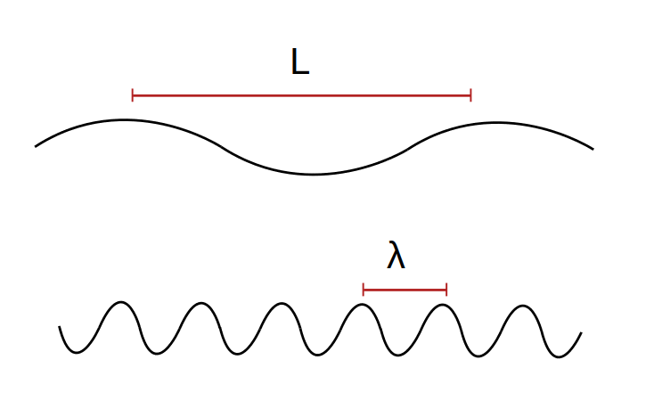
Figure 1: Sketch of a perturbed spacetime in the geometric-optics regime. $L$ is the characteristic length of the background and $\lambda$ is the wavelength of the perturbation.

Let us split the spacetime metric as

$$g_{\alpha\beta}=g^{B}_{\alpha\beta}+\epsilon h_{\alpha\beta}+\epsilon^{2}j_{\alpha\beta}+\mathcal{O}(\epsilon^{3}),$$ (171)

where $g^{B}_{\alpha\beta}$ is unperturbed background metric, while $h_{\alpha\beta}$ and $j_{\alpha\beta}$ are the first and second order perturbations ($\epsilon$ being a small parameter). Let us then consider the vacuum Einstein equations $G_{\alpha\beta}=0$, and expand them in $\epsilon$ as

$$0=G_{\alpha\beta}[g^{B}]+\epsilon G^{(1)}_{\alpha\beta}[h,g^{B}]+\epsilon^{2}\Big{(}G^{(1)}_{\alpha\beta}[j,g^{B}]+G^{(2)}_{\alpha\beta}[h,g^{B}]\Big{)}.$$ (172)

Here, the first term is the Einstein tensor computed with the background metric, the second one gives the equations of motion for the first order perturbations (c.f. section (II.2)), while the $\epsilon^{2}$ term gives the equations of motion for the second order perturbations (which are in turn comprised of terms quadratic in $h$, denoted by $G_{\alpha\beta}^{(2)}[h,g^{B}]$, and terms linear in $j$, denoted by $G^{(1)}_{\alpha\beta}[j,g^{B}]$).

Taking now an average of this equation, one can note that since $G^{(1)}[\ldots,g^{B}]$ is a linear operator (the linearized Einstein tensor on the background metric), the average commutes with it, giving therefore $\langle G^{(1)}_{\alpha\beta}[h,g^{B}]\rangle=G^{(1)}_{\alpha\beta}[\langle h\rangle,g^{B}]=0$ (because the first order perturbations are oscillatory and thus average to zero, cf. section (II.2)). Similarly, $\langle G^{(1)}_{\alpha\beta}[j,g^{B}]\rangle=G^{(1)}_{\alpha\beta}[\langle j\rangle,g^{B}]$, where we are allowing for $\langle j\rangle\neq 0$. In fact, the second order equations of motion have the cartoon form $\Box j_{\alpha\beta}={\cal O}(h)^{2}$, i.e. second order perturbations are sourced by products of first order ones. As such, the average of the second order perturbations cannot be zero as $\langle{\cal O}(h)^{2}\rangle$ will not vanish, in general. The average of Eq. (172) thus yields

$$0=G_{\alpha\beta}[g^{B}]+\epsilon^{2}\Big{(}G^{(1)}_{\alpha\beta}[\langle j\rangle,g^{B}]+\langle G^{(2)}_{\alpha\beta}[h,g^{B}]\rangle\Big{)}\,,$$ (173)

where we have used the fact that $\langle G_{\alpha\beta}[g^{B}]\rangle=G_{\alpha\beta}[g^{B}]$ since the background metric varies on scales much larger than those on which the average is performed. This equation can then be written, by resumming the Taylor expansion, as

$$G_{\mu\nu}[g^{B}+\epsilon^{2}\langle j\rangle]=8\pi GT_{\mu\nu}^{\rm GW},$$ (174)

with

$$T^{\rm GW}_{\mu\nu}=-\frac{1}{8\pi}\langle G_{\mu\nu}^{(2)}[h,g^{B}]\rangle,$$ (175)

To compute this average, one can write $G_{\mu\nu}^{(2)}[h,g^{B}]$ explicitly, use the fact that covariant derivatives commute up to terms depending on the Riemann tensor, and show that these terms are subleading in the geometric-optics regime $\lambda\ll L$. A more detailed calculation can be found in Flanagan:2005yc and misner1973gravitation and and yields (for transverse traceless perturbations)

$$T_{\alpha\beta}^{\rm GW}=\frac{1}{32\pi}\langle\nabla_{\alpha}h^{\mathrm{TT}}_{\rho\sigma}\nabla_{\beta}h_{\mathrm{TT}}^{\rho\sigma}\rangle.$$ (176)

Remarkably, this is the same result that we derived previously, except for the average, which shows explicitly that the stress-energy tensor of gravitational waves is a non-local object (i.e. it makes no sense to define the stress-energy tensor of gravitational waves pointwise, but only on scales larger than the wavelength). Just as the gravitational force disappears for an observer in a free-falling elevator if the elevator is much smaller than the Earth (otherwise non-local tidal effects appear, cf. Eq. (159)), the gravitational wave perturbation can be set to zero by going to RNCs locally, but only on scales smaller than the spacetime curvature radius (which is given by $\lambda$ for the perturbed spacetime represented in Fig. (1)).

V.1 The gravitational contribution to the mass of a compact star

In this section we will take a short detour and investigate another example showing that the gravitational field, although it can be set to zero locally, provides a finite contribution to the energy of the system on non-local scales. We will consider indeed a compact spherically symmetric star, and compute the contribution of the gravitational field to its mass.

Let us start by modeling the metric as

$$ds^{2}=-B(r)dt^{2}+A(r)dr^{2}+r^{2}d\Omega^{2},$$ (177)

and the matter by a perfect fluid. The Einstein equations and the conservation of the fluid’s stress energy tensor then yield (assuming asymptotic flatness) the famous Tolman-Oppenheimer-Volkoff equations Shapiro:1983du :

$$\frac{dp}{dr}=-\rho\frac{m(r)}{r^{2}}\Bigg{(}1+\frac{p}{\rho}\Bigg{)}\Bigg{(}1+\frac{4\pi r^{3}p}{m(r)}\Bigg{)}\Bigg{(}1-\frac{2m(r)}{r}\Bigg{)}^{-1},$$ (178)

$$\frac{1}{2B}\frac{dB}{dr}=-\frac{1}{p+\rho}\frac{dp}{dr},$$

$$A(r)=\frac{1}{1-\frac{2m(r)}{r}},$$

where

$$m(r)=\int^{r}_{0}\rho(r^{\prime})4\pi r^{\prime 2}dr^{\prime}.$$

Clearly, the first equation is the relativistic Euler equation, where $\frac{p}{\rho}$, $\frac{4\pi r^{3}p}{m(r)}$ and $\frac{2m(r)}{r}$ are the relativistic corrections, which disappear in the Newtonian limit $c\rightarrow\infty$ (if $c$ is reinstated). As can be seen, the solution to these equations reduces to the Schwarzschild metric in vacuum (and thus in the exterior of the star). In particular, the metric in the exterior is given by the Schwarzschild metric with mass $m(\infty)=\int^{R}_{0}\rho(r^{\prime})4\pi r^{\prime 2}dr^{\prime}$, where $R$ is the radius of the star. This mass can be interpreted as the star’s gravitational mass, as measured by an observer that were to fly satellites far from the star and interpret their motion with Kepler’s law. More formally, one can show that this mass matches the Arnowitt-Deser-Misner mass of the spacetime (which in turn matches its Komar mass), see e.g. townsend ; wald .

The total baryonic mass of the star can instead be obtained from the continuity equation for the baryonic current $j^{\mu}=m_{b}nu^{\mu}$, where $m_{b}$ is the average baryon mass and $n$ is the baryon number density. The baryonic mass is then

$$M_{b}=\int\mathrm{d}x^{3}\sqrt{-g}j^{t}=m_{b}\int 4\pi r^{2}\sqrt{A(r)}n(r)dr\,.$$ (179)

This mass corresponds to the sum of the rest masses of all the baryons of the system, but does not include the internal energy. Since the internal energy density of a fluid is given by the difference $\rho-m_{b}n$, we would expect the total mass of the system to be given simply by

$$M_{\star}=\int 4\pi r^{2}\sqrt{A(r)}\rho(r)dr\,.$$ (180)

This mass, however, still differs from $m(\infty)$. To understand this discrepancy one may compute the difference between the two, reinstate factors of $G$ and $c$ (using e.g. dimensional analysis) and expand it in orders of $1/c^{2}$. Equivalently, one can expand the difference in the weak gravity limit $m(r)/r\ll 1$. By using the fact that $A(r)=[1-2Gm(r)/(rc^{2})]^{-1}$, one then finds

$$m(\infty)-M_{\star}=-\int\mathrm{d}r\frac{4\pi r^{2}\rho(r)Gm(r)}{rc^{2}}=U_{\rm self}/c^{2}\,,$$ (181)

$$U_{\rm self}=-G\int\mathrm{d}m(r)\frac{m(r)}{r}\,.$$ (182)

This shows (i) that the gravitational mass $m(\infty)$ is always smaller than the expected value $M_{\star}$, and (ii) that in the Newtonian limit the difference is given exactly by the contribution of the (Newtonian) gravitational self-energy, i.e. (in absolute value) the work that one would need to perform against the gravitational force to destroy the star. Once again, we have found that even though it can be locally set to zero, the gravitational field does contribute to the mass of an extended object. This contribution is of the order of $10-20\%$ for neutron stars.

VI The inspiral and merger of binary systems of compact objects

In this section we will use the results that we have derived to gain some semi-quantitative understanding of the physics of binary systems of compact objects (black holes and neutron stars).

Let us first apply the quadrupole formula to a system of two compact objects with masses $m_{1}$ and $m_{2}$ on a circular orbit of radius $r$ and orbital frequency $\Omega$, which at lowest (i.e. Newtonian) order is given by Kepler’s law

$$\Omega=\sqrt{\frac{M}{r^{3}}}\,,$$ (183)

with $M=m_{1}+m_{2}$. The gravitational wave signal predicted by the quadrupole formula, for an observer at distance $D$ and angle $\iota$ with respect to the direction orthogonal to the orbital plane, then reads

$$h^{\rm TT}_{ij}=h\left[\begin{matrix}\frac{1+\cos^{2}\iota}{2}\cos 2\Omega t&\cos\iota\sin 2\Omega t&0\cr\cos\iota\sin 2\Omega t&-\frac{1+\cos^{2}\iota}{2}\cos 2\Omega t&0\cr 0&0&0\cr\end{matrix}\right]$$ (184)

with the amplitude (also referred to as “strain”) being

$$h=\frac{4\mu\Omega^{2}r^{2}}{D}=\frac{4\mu M^{2/3}\Omega^{2/3}}{D}\;,$$ (185)

where we have also introduced the reduced mass $\mu=m_{1}m_{2}/M$.

Several comments are worth making here. First, the frequency of the gravitational wave signal is twice the orbital frequency. This is due to the tensor nature of gravitational waves. By reinstating $G$ and $c$ (recalling that $h$ must be dimensionless) and computing explicitly the amplitude, one finds e.g. a strain of $\sim 10^{-22}$ for a system of two neutron stars of masses $m_{1}=m_{2}=1.4M_{\odot}$, orbital period of 10 ms and distance of 50 Mpc. Similarly, a strain $h\sim 10^{-21}$ can be obtained e.g. for an equal mass binary of black holes of 30 $M_{\odot}$ each, at a distance of 400 Mpc and with the same orbital period of 10 ms. Clearly, these sources have gravitational wave frequencies $\sim 100$ Hz, and as we will see they are detectable by current ground based interferometers (LIGO-Virgo-KAGRA). Similarly, typical sources in the bands of LISA (mHz) and pulsar-timing arrays (nHz) are e.g. a binary of massive black holes of $10^{7}M_{\odot}$ each, with period of a few hours and distance of few Gpc ($h\sim 10^{-16}$) or a binary of supermassive black holes of $10^{9}M_{\odot}$ each, with period of one year and distance $\sim 1$ Gpc ($h\sim 10^{-15}$), respectively. Note how small the amplitude of these metric perturbations is compared to the amplitude of the metric perturbation at the surface of the Sun, $h\sim GM_{\odot}/(R_{\odot}c^{2})\sim 10^{-6}$. Another important observation is that the strain decays as $1/D$. This is why gravitational wave observations allow for exploring the Universe up to high redshift. Not only do gravitational waves interact very weakly with matter (since the interaction is only gravitational), but interferometers detect directly the gravitational wave strain $h$, which decays more slowly than the electromagnetic fluxes ($\propto 1/d^{2}$) collected e.g. by optical telescopes.

Using now Eq. (185) in the stress energy tensor of gravitational waves, one can get the gravitational wave flux $T^{\rm GW}_{ti}$. Like all fluxes, this decays as $1/D^{2}$, but we stress again that interferometers observe $h$ directly, and not the flux. Integrating the flux on a sphere far from the source, one finds that the gravitational wave luminosity of a binary (i.e. the energy carried away by gravitational waves per unit time) takes the simple form

$$\dot{E}_{\rm GW}=\frac{32}{5}\frac{G}{c^{3}}\Bigg{(}\frac{Gm_{1}m_{2}}{r^{2}}\Bigg{)}^{2}\Bigg{(}\frac{v}{c}\Bigg{)}^{2}\,,$$ (186)

where we have explicitly reinstated $G$ and $c$. The energy that gravitational waves remove from the source must of course come from the system’s kinetic and potential energy. For a circular Keplerian binary, the sum of kinetic and potential energy is simply given, in the center of mass frame, by

$$E_{\rm tot}=\frac{1}{2}\mu v^{2}-\frac{GM\mu}{r}=-\frac{1}{2}\frac{GM\mu}{r}\,.$$ (187)

By requiring energy conservation ($\dot{E}_{\rm tot}=-\dot{E}_{\rm GW}$), one can then obtain an expression of the rate of change of the separation, $\dot{r}$, due to gravitational wave emission. Clearly $\dot{r}<0$, i.e. the binary slowly spirals in under the backreaction of gravitational waves. This can of course be interpreted as a PN contribution to the acceleration of the system, i.e.

$$\vec{a}_{12}=\vec{a}_{N}\Big{(}1+\mathcal{O}\Big{(}\frac{1}{c^{2}}\Big{)}+\mathcal{O}\Big{(}\frac{1}{c^{4}}\Big{)}+\mathcal{O}\Big{(}\frac{1}{c^{5}}\Big{)}\Big{)},$$ (188)

where $\vec{a}_{N}$ is the Newtonian acceleration, $\mathcal{O}(\frac{1}{c^{2}})$ is the 1PN (conservative) correction, $\mathcal{O}(\frac{1}{c^{4}})$ is the 2PN (conservative) correction and $\mathcal{O}(\frac{1}{c^{5}})$ is the 2.5PN (dissipative) backreaction of gravitational waves. Note that the $\mathcal{O}(\frac{1}{c^{5}})$ scaling of the last term follows from the factors of $1/c$ in Eq. (186).

Using Kepler’s law, $\dot{r}$ can be recast into the rate of change of the orbital angular frequency, $\Omega$. Using then the relation between gravitational wave frequency and $\Omega$, $f=2f_{\rm orb}=\Omega/\pi$, one finally obtains

$$\dot{f}=\frac{96}{5}\frac{1}{c^{5}}\pi^{8/3}(GM_{c})^{5/3}f^{11/3}\,,$$ (189)

where we have introduced the chirp mass

$$M_{c}=M\eta^{3/5},$$ (190)

where $\eta=\frac{\mu}{M}$ is the symmetric mass ratio. The chirp mass is indeed the quantity that can be most easily estimated from the gravitational wave signal from inspiraling binaries: as gravitational waves remove energy and angular momentum, the binary spirals in, the separation decreases, and the frequency of gravitational waves increases depending on $M_{c}$ alone (at leading PN order). This expression can also be recast into an equation for the rate of change of the orbital period. The latter is the quantity monitored in binary pulsar systems, i.e. systems at least one component of which is a millisecond pulsar. The presence of the pulsar allows for tracking the period of the binary system with exquisite accuracy, historically providing for the first time evidence for the existence of gravitational waves Taylor:1979zz .

In order to gain more qualitative understanding of the inspiral phase beyond the leading PN order, we will now make a short detour and recall the most salient features of geodesic orbits in Schwarzschild and Kerr spacetimes. While this is only applicable to binaries with very small mass ratio $q=m_{2}/m_{1}\ll 1$, the qualitative features that we will discover (e.g. the effect of spins, the plunge) will survive even at mass ratios $q\approx 1$. This is somewhat expected from Newtonian mechanics, where one can map a binary with arbitrary masses into a particle with the reduced mass $\mu$ around a particle with the total mass $M$, but it is not at all obvious in GR. Only recently has evidence started accumulating that a similar mapping between arbitrary binaries and the test-particle limit may exist even in PN theory, although approximately. This approximate mapping goes under the name of ‘effective-one-body’ model eob .

VI.1 Geodesics in Schwarzschild and Kerr

Let us start by studying geodesics in the Schwarzschild spacetime, whose line element we write in areal coordinates in the usual form

$$\mathrm{d}s^{2}=-\left(1-2\frac{M}{r}\right)\mathrm{d}t^{2}+\frac{\mathrm{d}r^{2}}{1-2M/r}+r^{2}\mathrm{d}\Omega^{2}\,.$$ (191)

Since the metric is static and spherically symmetric, we can look at equatorial geodesics without loss of generality (i.e. the coordinates can always be chosen to be such that orbits have $\theta=\frac{\pi}{2}$).

Let us start with particles having non-zero mass (timelike geodesics). From the existence of the two Killing vectors $\partial_{t}$ and $\partial_{\phi}$, it follows that the specific  energy and angular momentum observed at infinity, i.e. $E=-u_{t}$ and $L=u_{\phi}$ with $u^{\mu}=\mathrm{d}x^{\mu}/\mathrm{d}\tau$ the four-velocity, are conserved. One can then obtain the first-order equations

$$\left(1-\frac{2M}{r}\right)\frac{\mathrm{d}t}{\mathrm{d}\tau}=E,$$ (192)

$$r^{2}\frac{\mathrm{d}\phi}{\mathrm{d}\tau}=L\,.$$

Moreover, by using these equations in the conservation of the norm $u^{\mu}u_{\mu}=-1$, one can obtain a first-order equation for the radial motion:

$$\frac{1}{2}\left(\frac{\mathrm{d}r}{\mathrm{d}\tau}\right)^{2}+V(r)=\frac{1}{2}E^{2},$$ (193)

with the effective potential being given by

$$V(r)=\frac{1}{2}-\frac{M}{r}+\frac{L^{2}}{2r^{2}}-\frac{ML^{2}}{r^{3}}\,.$$ (194)

Apart from the first (constant and thus irrelevant) term, this potential includes the Newtonian potential, the usual Newtonian centrifugal term, but the last term does not appear in Newtonian mechanics. In fact, it is a 1PN term, as can be seen by reinstating $c$ by dimensional analysis.

As a consequence of this term, the behavior of the potential at small $r$ drastically differs from the Newtonian one. Unlike the latter, which predicts the existence of stable circular orbits down to arbitrarily small radii, Eq. (194) predicts the existence of an innermost stable circular orbit (ISCO) at $r=6M$. This can be seen by solving the equations defining circular orbits, $E^{2}/2-V(r)=V^{\prime}(r)=0$, and checking the sign of $V^{\prime\prime}(r)$ to assess stability. As can also be understood by plotting $V$, for $E>1$ only unstable circular orbits exist. However, for each value of $E<1$ (corresponding to bound orbits) two circular orbits exist, with the one at larger radius being stable and the other being unstable. These orbits exist only for $L\geq 2\sqrt{3}M$ and coincide for $L=2\sqrt{3}M$, which corresponds to the ISCO ($r=6M$ and $E=2\sqrt{2}/3$). The unstable circular orbits lie instead at $r<6M$, but they always have $r>3M$ (they only approach $r=3M$ in the ultra-relativistic limit $E,L\to\infty$).

By redoing the same analysis for null orbits, one can prove that the radial motion obeys

$$\frac{1}{E^{2}}\left(\frac{dr}{d\lambda}\right)^{2}=-V_{\rm ph}=1-\frac{b^{2}}{r^{2}}\left(1-\frac{2M}{r}\right),$$ (195)

where $\lambda$ is an affine parameter and $b=L/E$ is usually referred to as impact parameter. An analysis of the effective potential $V_{\rm ph}$ shows that a circular orbit exists only for a critical value of $b$, namely $b=3\sqrt{3}M$. This circular null orbit (also known as light ring) lies at a radius of $r=3M$ and is unstable. Its existence and properties are not only important for the interpretation of the observations by the Event Horizon Telescope (EHT) eht , but also for the physics of black hole quasinormal modes, as we will see in the following.

The case of geodesics in a Kerr spacetime is slightly more involved, because one can no longer assume equatorial motion due to the absence of spherical symmetry. In Boyer-Lindquist coordinates the metric reads

$$ds^{2} = -\left(1-\frac{2Mr}{\Sigma}\right)~{}dt^{2}+\frac{\Sigma}{\Delta}~{}dr^{2}+\Sigma~{}d\theta^{2}$$ (196)

$$+\left(r^{2}+a^{2}+\frac{2Ma^{2}r}{\Sigma}\sin^{2}\theta\right)\sin^{2}\theta~{}d\phi^{2}-\frac{4Mar}{\Sigma}\sin^{2}\theta~{}dt~{}d\phi,$$

where $a=S/M$ (with $S$ the spin), $M$ is the mass and

$$\Sigma=r^{2}+a^{2}\cos^{2}\theta,\quad\Delta=r^{2}-2Mr+a^{2}.$$ (197)

The Killing vectors $\partial_{t}$ and $\partial_{\phi}$ still exist, and imply that the specific energy $E=-u_{t}$ and angular momentum (in the spin direction) $L=u_{\phi}$ must be conserved. However, one more conservation equation (besides the unit norm condition) is needed to reduce the equations of motion to first order. Fortunately, the Kerr geometry has a ‘hidden’ symmetry, which can be described by a Killing-Yano tensor. This symmetry implies the existence of an additional constant of motion, the Carter constant $Q$, which allows for writing the equations for timelike geodesics (with particle mass $\mu$) as

$$\left(\frac{dr}{d\lambda}\right)^{2}=V_{r}(r), \frac{dt}{d\lambda}=V_{t}(r,\theta),$$

$$\left(\frac{d\theta}{d\lambda}\right)^{2}=V_{\theta}(\theta), \frac{d\phi}{d\lambda}=V_{\phi}(r,\theta)\;,$$ (198)

with

$$V_{t}(r,\theta)\equiv E\left(\frac{\varpi^{4}}{\Delta}-a^{2}\sin^{2}\theta\right)+aL\left(1-\frac{\varpi^{2}}{\Delta}\right),$$ (199a)

$$V_{r}(r)\equiv\left(E\varpi^{2}-aL\right)^{2}-\Delta\left[r^{2}+(L-aE)^{2}+Q\right],$$ (199b)

$$V_{\theta}(\theta)\equiv Q-L^{2}\cot^{2}\theta-a^{2}(1-E^{2})\cos^{2}\theta,$$ (199c)

$$V_{\phi}(r,\theta)\equiv L\csc^{2}\theta+aE\left(\frac{\varpi^{2}}{\Delta}-1\right)-\frac{a^{2}L}{\Delta},$$ (199d)

where we have defined

$$\varpi^{2}\equiv r^{2}+a^{2}$$ (200)

and the “Carter time” $\lambda$ by

$$\frac{d\tau}{d\lambda}\equiv\Sigma\;.$$ (201)

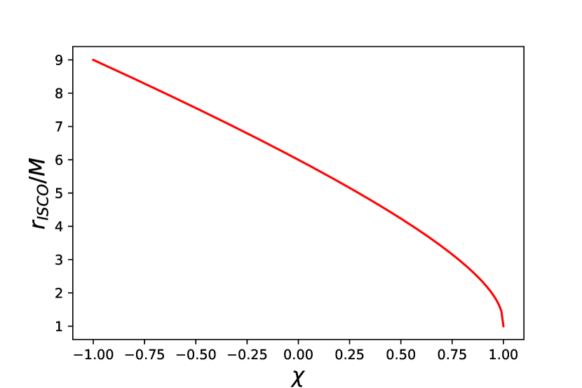
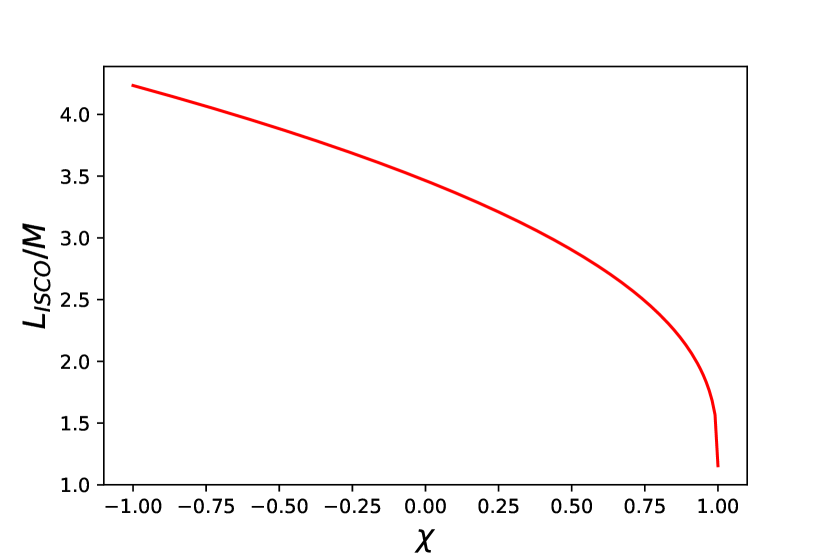
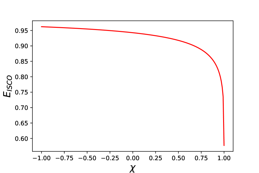
Figure 2: ISCO radius, specific angular momentum and specific energy for equatorial orbits in Kerr.

The most striking difference from the Schwarzschild case is the presence of a non-trivial equation for the angular variable $\theta$, which describes the precession of the orbital angular momentum of the particle around the spin of the Kerr geometry. Moreover, the spin parameter $a$ also enters the effective potential for the radial motion. This has profound implications for the particle’s motion. Focusing for instance on non-precessing (i.e. equatorial) orbits, we can set $\theta=\pi/2$ and $Q=0$, and we can obtain the radius, specific energy and specific angular momentum of circular orbits by solving $V_{r}(r)=V^{\prime}_{r}(r)=0$. Like in the Schwarzschild case, this analysis shows the existence of an ISCO, whose properties depend on the spin as Bardeen:1972fi

$${E}_{{}_{\rm ISCO}}(\chi)=\sqrt{1-\frac{2}{3{r}_{{}_{\rm ISCO}}(\chi)}}\,,$$ (202)

$${L}_{{}_{\rm ISCO}}(\chi)=\frac{2}{3\sqrt{3}}\left[1+2\sqrt{3{r}_{{}_{\rm ISCO}}(\chi)-2}\right]\,,$$ (203)

$${r}_{{}_{\rm ISCO}}(\chi)=3+Z_{2}-\frac{\chi}{|\chi|}\sqrt{(3-Z_{1})(3+Z_{1}+2Z_{2})}\,,$$ (204)

$$Z_{1}=1+(1-\chi^{2})^{1/3}\left[(1+\chi)^{1/3}+(1-{\chi})^{1/3}\right]\,,$$ (205)

$$Z_{2}=\sqrt{3{\chi}^{2}+Z_{1}^{2}}\,,$$ (206)

where $\chi=a/M$. The parameter $\chi$ ranges from -1 to 1, with positive values corresponding to orbits co-rotating with the Kerr black hole, while negative values correspond to counter-rotating orbits. In the limit $\chi\to 0$, these expressions reduce to those for the Schwarzschild ISCO.

The dependence of these expressions on the spin is a special case of a more general phenomenon appearing in GR, the dragging of inertial frames or Lense-Thirring effect. Unlike what happens in Newtonian theory, the spin has a clear impact on the dynamics, “dragging” matter into rotation. In accordance with this, Eqs. (202)–(206) predict that as the spin increases in magnitude, prograde orbits (i.e. ones co-rotating with the Kerr black hole) have smaller and smaller ISCO radii, down to ${r}_{{}_{\rm ISCO}}=M$ in the extremal limit $\chi=1$.  As a result, the values of ${E}_{{}_{\rm ISCO}}$ and ${L}_{{}_{\rm ISCO}}$ decrease as $\chi$ grows from 0 to 1. For retrograde orbits ($\chi<0$) the ISCO instead moves to larger radii as the spin magnitude increases, up to $r=9M$ in the extreme limit. As a consequence, the values of ${E}_{{}_{\rm ISCO}}$ and ${L}_{{}_{\rm ISCO}}$ increase as $\chi$ goes from 0 to -1. These behaviors are shown in Fig. (2).

For a photon in the Kerr geometry, the geodesics equations are instead Bardeen:1972fi

$$\left(\frac{dr}{d\tilde{\lambda}}\right)^{2}=V_{r}(r), \frac{dt}{d\widetilde{\lambda}}=V_{t}(r,\theta),$$

$$\left(\frac{d\theta}{d\widetilde{\lambda}}\right)^{2}=V_{\theta}(\theta), \frac{d\phi}{d\widetilde{\lambda}}=V_{\phi}(r,\theta)\;,$$ (207)

with $\widetilde{\lambda}$ a “time” parameter, $b=L/E$, $q=Q/E^{2}$, and

$$\widetilde{V}_{t}(r,\theta)\equiv\frac{-a^{2}\Delta\sin^{2}\theta+ab(\Delta-\varpi^{2})+\varpi^{4}}{\Delta}$$ (208a)

$$\widetilde{V}_{r}(r)\equiv(\varpi^{2}-ab)^{2}-\Delta\left[(a-b)^{2}+q\right],$$ (208b)

$$\widetilde{V}_{\theta}(\theta)\equiv a^{2}\cos^{2}\theta-b^{2}\cot^{2}\theta+q,$$ (208c)

$$\widetilde{V}_{\phi}(r,\theta)\equiv\frac{b}{\sin^{2}\theta}-\frac{a(ab+\Delta-\varpi^{2})}{\Delta}\,.$$ (208d)

Specializing again to equatorial orbits ($q=0$, $\theta=\pi/2$), one finds, like in Schwarzschild, that there exists an unstable circular photon orbit, whose coordinate radius reads Bardeen:1972fi

$$r_{\rm ph}(\chi)=2M\{1+\cos[2/3\arccos(-\chi)]\}\,.$$ (209)

This is plotted in Fig. (3), together with the orbital frequency $\Omega_{\rm ph}=\mathrm{d}\phi/\mathrm{d}t$ (obtained from Eq. (208)). As can be seen, the frame dragging once again makes the photon orbit radius decrease with $\chi$, with $r_{\rm ph}\to M$ as $\chi\to 1$.  Like in the Schwarzschild case, not only are circular photon orbits relevant for EHT observations, but also for the physics of quasinormal modes, as we will see below.

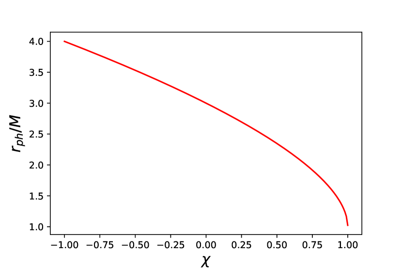
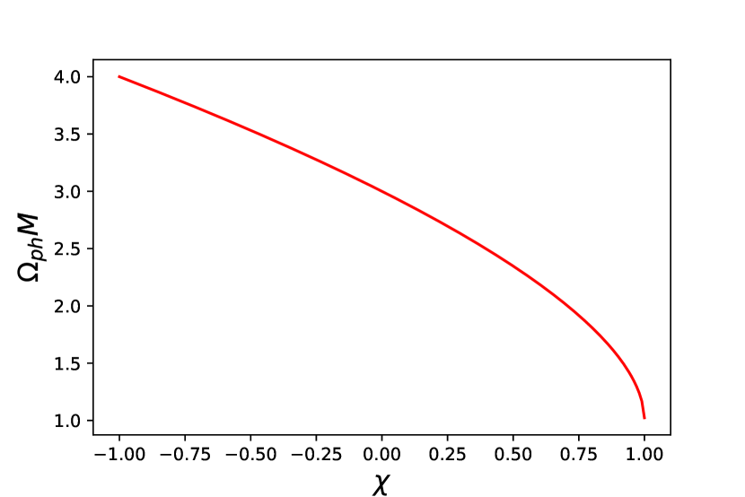
Figure 3: Circular photon orbit’s radius and orbital frequency for equatorial orbits in Kerr.

VI.2 A qualitative description of the inspiral and merger

Let us now utilize what we have learned so far to gain some qualitative understanding of the evolution of a quasi-circular binary of compact objects (black holes or neutron stars). As have seen, gravitational waves are emitted and carry energy and angular momentum away from the system. As a result, the separation of the binary decreases and the orbital frequency increases. The rates of change of these quantities, as we have seen, only depend on a combination of the two masses, the chirp mass, at leading PN order. However, at higher PN orders the gravitational wave fluxes also depend on the individual masses and spins. PN corrections also appear in the conservative sector, changing e.g. the relation between the orbital frequency and the system parameters (which is only given by Kepler’s law at Newtonian order, cf. sections (III) and (VI.1)), giving rise to precession (if at least one spin is non-zero and misaligned with the orbital angular momentum, cf. section (VI.1)), etc. Precession (spin-spin and spin-orbit) introduces modulations in the gravitational waveforms (both in amplitude and phase), as shown for instance in Fig. (4). This makes measurements of the spin directions possible (at least in principle) with gravitational wave detectors.

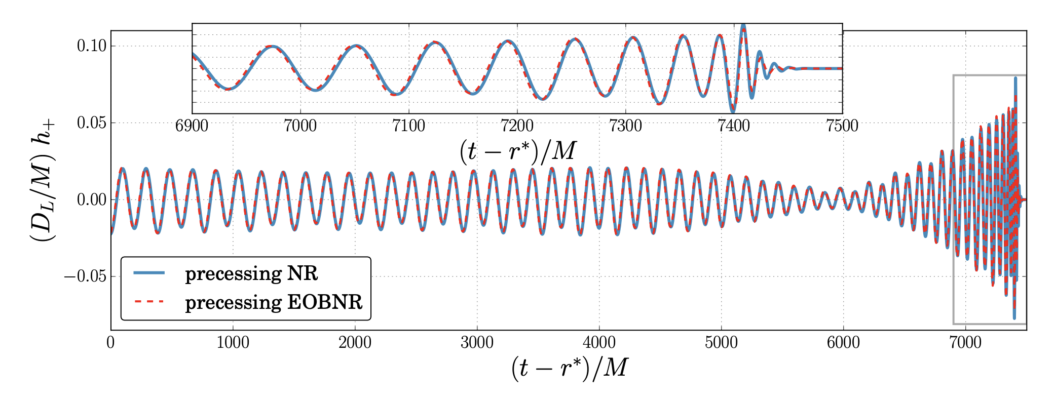
Figure 4: Two waveform approximants for the signal $h_{+}$ (normalized by the luminosity distance $D_{L}$ and the system’s total mass $M$) produced by a black hole binary with mass ratio $1:5$, spin parameters 0.5 and 0 (for the heavier and lighter object respectively, and with the non-vanishing spin initially in the orbital plane) as function of retarded time. The observer is located 60 degrees away from the orbital angular momentum axis. Taken from Ref. eobprec

As the binary’s separation shrinks, the system transitions from one circular orbit to the next until it either reaches the ISCO or the two bodies touch. We have seen that an ISCO exists in the test-particle limit (i.e. for geodesics), but a similar transition to unstable circular orbits occurs also for comparable-mass binaries of black holes LeTiec:2011dp (neutron stars touch and interact before they reach this effective ISCO). When the separation reaches the effective ISCO, or when the two bodies touch (in the case of neutron stars), the binary plunges and merges. The merger phase can only be studied via numerical-relativity simulations, but at least for black holes the post-merger phase can be understood analytically in terms of quasi-normal modes, as we will see in the next section. As for neutron stars, the post-merger phase depends critically on the microphysics (e.g. on the equation of state of nuclear matter) and can only be predicted via numerical simulations.

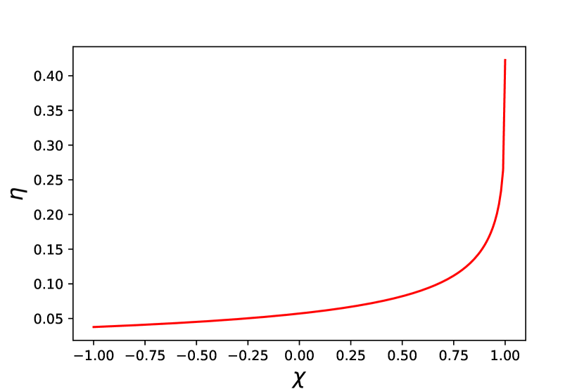
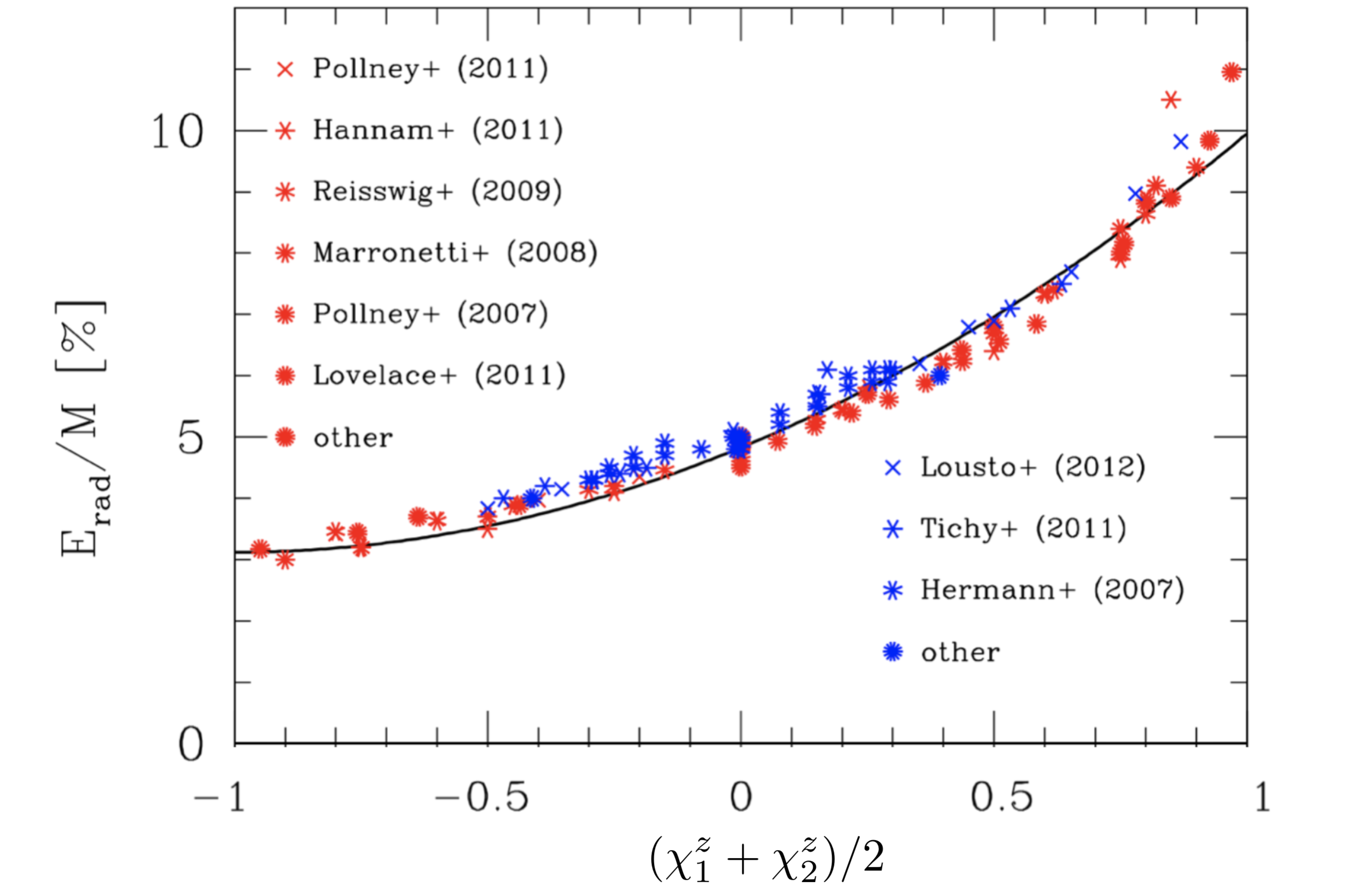
Figure 5: Top: The radiative efficiency of a geometrically thin, optically thick accretion disk around a Kerr black hole with spin parameter $\chi$. Note that the maximum spin expected for black holes surrounded by such accretion disks is $\chi=0.998$ thorne , for which the efficiency is $\approx 32\%$. Bottom: the fraction of the total mass $M=m_{1}+m_{2}$ emitted by a black hole binary system in gravitational waves, as a function of the average of the projections of the two spins on the orbital angular momentum axis, $(\chi_{1}+\chi_{2})/2$. (Adapted from Ref. morozova .)

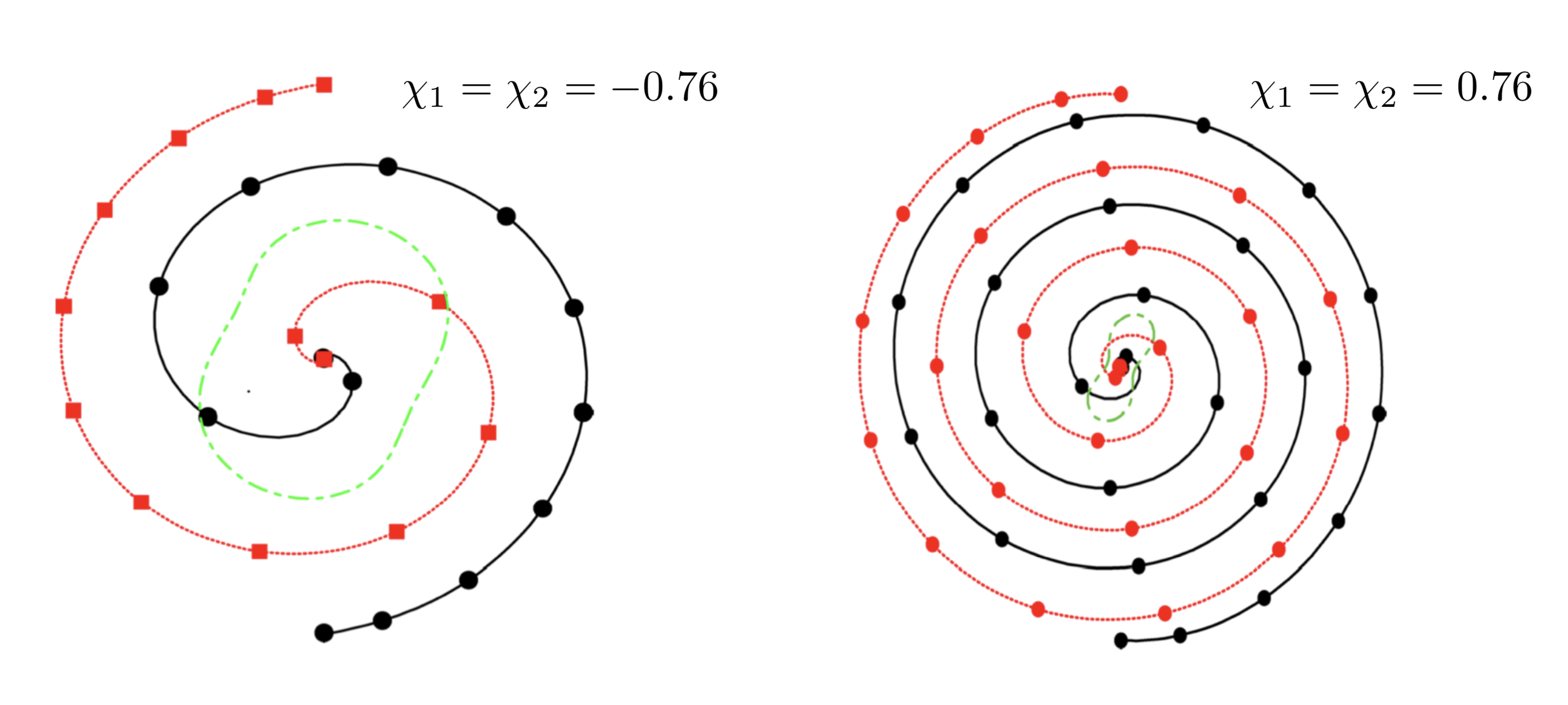
Figure 6: Numerical relativity simulations of binary black holes with spins $|\chi_{1}|=|\chi_{2}|=0.76$ either antialigned (left) or aligned (right) with the orbital angular momentum. The squares and circles represent the puncture positions every 10 $M$ (with $M=m_{1}+m_{2}$) of evolution, and the lines joining them can therefore be thought as the trajectories of the black holes. The dashed green circles represent the first common apparent horizon.

The position of the effective ISCO, just like in the test-particle limit, depends critically on the spins of the two objects. The larger the spins, the more the effective ISCO moves inwards and the longer the binary emits gravitational waves before plunging. This is exactly the same effect that takes place, in the electromagnetic case, for geometrically thin, optically thick accretion disks. In the latter, the gas spirals in on quasi-circular orbits, as it loses energy because of friction with the neighboring gas elements. The gas potential and kinetic energy is thus converted into heat, and eventually radiated away (e.g. in the optical, infrared, UV and/or X-ray bands). This process can only continue, however, until the gas reaches the ISCO of the central black onto which it is accreting. For a gas element with unit mass starting at rest at infinity, the energy when it reaches the ISCO is $E_{{}_{\rm ISCO}}$ (as given by Eq. (202)). By energy conservation, the radiative efficiency of an accretion disk is therefore $\eta=1-E_{{}_{\rm ISCO}}$, which is a strong function of spin, as can be seen from Fig. (5) (top panel).

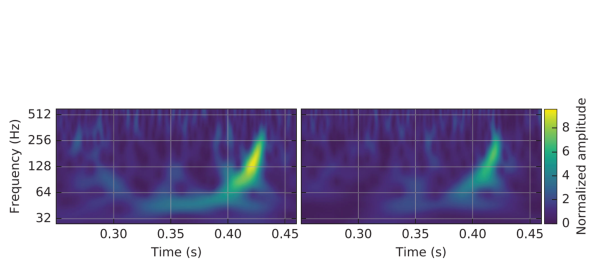
Figure 7: A spectrogram of the GW150914 event observed by LIGO Hanford (left) and Livingston (right). The color code represents the normalized strain amplitude. Figure adapted from Ref. GW150914 .

Computing a similar efficiency for gravitational waves from binary systems is not easy away from the test-particle limit, as the effective ISCO energy is not known analytically for comparable masses. However, one can perform numerical relativity simulations, which show in fact exactly the same effect (qualitatively). Fig. (6), taken from Ref. campanelli , shows the “trajectories” (in some sense) of two black holes with spins respectively aligned (right) and antialigned (left) with the orbital angular momentum. It can be visually seen that the orbit with aligned spins (corresponding to prograde Kerr geodesics) reaches smaller separations and performs more cycles than that for antialigned spins (corresponding to retrograde Kerr geodesics). This effect is known in the literature as “orbital hang up”, but it is really a manifestation of the frame dragging of GR. The same effect can be seen at play in Fig. (5) (bottom panel), adapted from Ref. morozova , which collected the energy emitted in gravitational waves in various black hole binaries simulated in the literature, and plotted it as function of a combination of the two spins (projected on the orbital angular momentum axis). Although the emission efficiency tops at about 10% at high spins, thus remaining lower than the electromagnetic efficiency shown in the top panel of Fig. (5), the behavior is qualitatively the same as the latter.

As a final application, let us show that the knowledge that we have gained so far, albeit qualitative, allows for interpreting the data of GW150914 GW150914 , the first direct gravitational wave detection, and for concluding that the components of this binary system must be black holes. A spectrogram of this event is shown in Fig. (7): the color code represents the gravitational wave strain amplitude in a given bin of time (x-axis) and frequency (y-axis). One can clearly recognize a “chirp”, i.e. an increase of the gravitational wave frequency with time, which one can fit with Eq. (189) to obtain $M_{c}\approx 30M_{\odot}$. This in turn implies, through Eq. (190), that the total mass must be $M\gtrsim 70M_{\odot}$. The power’s peak, which one expects to coincide with the plunge/merger phase, lies at $f\sim 150$ Hz. Translating that into an orbital frequency (dividing by a factor 2), and using Kepler’s law to convert to a separation (assuming for simplicity roughly equal masses), one finds that the plunge/merger takes place when the binary separation decreases to just 350 km. This is very close to the sum of the Schwarzschild radii of the two objects, $GM/c^{2}\gtrsim 210$ km. Therefore, the separation at which the plunge happens is comparable to the effective ISCO radius, which seems to favor the hypothesis that the two objects are black holes. In fact, if the objects were stars, they would touch, interact and plunge way before reaching the effective ISCO separation, i.e. the two objects must be very compact. Among compact objects – i.e. ones with $Gm/(Rc^{2})={\cal O}(1)$, with $m$ and $R$ the object’s mass and radius – the only options (in GR) are black holes and neutron stars. Neutron stars, however, are excluded because they cannot be more massive than $2-3M_{\odot}$. This leaves black holes as the only possibility.

VII The post-merger signal

As can be seen even in real strain data (c.f. Fig. (8) for the GW150914 event), after the amplitude peaks at the merger, the gravitational wave signal from a black hole binary seems to be well described by one (or more) damped sinusoids. This is in fact what happens, as can be understood rather easily by employing linear perturbation theory on a Schwarzschild or Kerr background, as we will do in this section. We will start with the simple toy problem of a test Klein-Gordon field on a Schwarzschild background, and we will then move to the case of gravitational perturbations on the same geometry. We will finally generalize the treatment to the Kerr case, which will allow for concluding that indeed the post-merger signal is well described by a linear superposition of quasi-normal modes of the final (spinning) black hole resulting from the merger. For more details, we refer the reader to the extensive review Berti:2009kk .

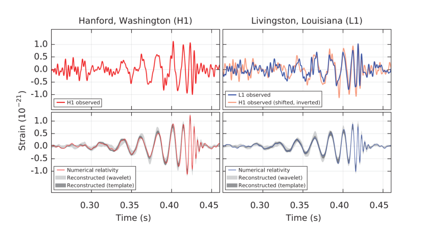
Figure 8: Top: the GW150914 data, as observed by the Hanford and Livingstone LIGO detectors. Bottom: the de-noised signal, reconstructed with template and wavelet techniques, alongside the prediction from numerical relativity simulations. Figure adapted from Ref. GW150914

VII.1 Scalar perturbations of non-spinning black holes

Let us start by considering the toy problem of a free scalar field on a Schwarzschild background, i.e. let us consider the Klein-Gordon equation

$$g^{\mu\nu}\nabla_{\mu}\nabla_{\nu}\varphi=0,$$ (210)

with $g^{\mu\nu}$ the contravariant components of the Schwarzschild metric given by Eq. (191). Since the metric is static and spherically symmetric, it is natural to decompose the scalar field in spherical harmonics ($Y_{\ell m}$) and Fourier modes ($e^{-i\omega t}$) as

$$\varphi=\sum_{\ell,m}\frac{R_{\ell m}(r)}{r}Y_{\ell m}(\theta,\phi)e^{-i\omega t},$$ (211)

where $R_{\ell m}$ characterizes the radial profile of the scalar field. By replacing this ansatz in the Klein-Gordon equation, that reduces to a single ordinary differential equation in the radial coordinate,

$$\frac{\mathrm{d}^{2}R_{\ell m}}{\mathrm{d}r_{*}^{2}}+\left(\omega^{2}-V_{\ell}\right)R_{\ell m}=0,$$ (212)

where

$$r_{*}\equiv r+2M\ln\left(\frac{r}{2M}-1\right),$$ (213)

is the tortoise coordinate and the potential $V_{\ell}$ the potential is given by

$$V_{\ell}(r)\equiv\left(1-\frac{2M}{r}\right)\left[\frac{\ell(\ell+1)}{r^{2}}+\frac{2M}{r^{3}}\right].$$ (214)

As can be seen, in the geometric optics (eikonal) limit $\ell\gg 1$ this potential reduces to the effective potential for the radial motion of photons, Eq. (195), if one identifies the impact parameter $b=L/E$ of photons with $\ell$. This is expected, since in the eikonal limit the wavefronts of a scalar field satisfying the Klein-Gordon equation move along null geodesics of the metric. We also stress that going from the partial differential equation (210) to the single ordinary differential equation (212) is highly non-trivial, and depends critically on the choice of the ansatz of Eq. (211).

To solve Eq. (212), we need to impose suitable boundary conditions. As $r_{*}\to\infty$, in order for nothing to enter the system, we need to impose outgoing boundary conditions $R_{\ell m}\sim\exp{(i\omega r_{*})}$. Conversely, since nothing can escape the horizon (which corresponds to $r_{*}\to-\infty$), we need to impose $R_{\ell m}\sim\exp{(-i\omega r_{*})}$ there (ingoing boundary conditions). Solving this boundary-value problem, one obtains a discrete spectrum of complex frequencies $\omega$. The corresponding excitations are referred to as quasinormal modes (as opposed to normal modes, which have real frequencies). Moreover, one can check that all frequencies in the spectrum have negative imaginary part, which corresponds to damped modes (c.f. Eq. (211)). This shows that a test scalar field is (linearly) stable on the Schwarzschild geometry.

Exercise 4: Plot the effective potential of Eq. (214) and approximate it qualitatively with a rectangular potential. Solve Eq. (212) in the three regions in which this rectangular potential is constant, and impose appropriate junction conditions at the transition radii and ingoing/outgoing boundary conditions at the horizon and at infinity. By counting the integration constants, show that the spectrum is discrete and complex. Solve numerically for a few frequencies in the spectrum.

VII.2 Tensor perturbations of non-spinning black holes

A similar analysis can be performed for the metric perturbation $h_{\mu\nu}$ of a Schwarschild spacetime. To exploit again the fact that the Schwarzschild geometry is static and spherically symmetric, we can decompose the time dependence in Fourier modes and the angular dependence in scalar, vector and tensor harmonics. In more detail, $h_{tt}$ $h_{tr}$, $h_{rr}$ are scalars on the two-sphere (i.e. under rotations), and can thus be expanded in the usual (scalar) spherical harmonics $Y_{\ell m}$. The cross terms $h_{tA}$ and $h_{rA}$ (with capital Latin letters spanning the two angles $\theta,\phi$) are instead vectors on the two sphere. A basis for vectors on the two-sphere can be obtained by taking gradients of the scalar harmonics,

$$Y^{{\cal E},\ell m}_{A}=\partial_{A}Y_{\ell m}\,,$$ (215)

or exterior derivatives of these gradients,

$$Y^{{\cal B},\ell m}_{A}=\epsilon_{A}^{\phantom{B}B}\partial_{B}Y_{\ell m}\,,$$ (216)

where $\epsilon_{AB}$ is the Levi-Civita tensor on the two-sphere and the angular indices are raised and lowered with the metric of the two-sphere, $\gamma_{AB}$:

$$\gamma_{AB}\mathrm{d}X^{A}\mathrm{d}X^{B}=\mathrm{d}\theta^{2}+\sin^{2}\theta\,\mathrm{d}\phi^{2}\,,$$ (217)

$$\epsilon_{AB}=\sqrt{\gamma}\,e_{AB}\,,$$ (218)

with $\gamma={\rm det}(\gamma_{AB})=\sin\theta$ and $e_{\theta\phi}=-e_{\phi\theta}=1$, $e_{\theta\theta}=e_{\phi\phi}=0$. Because scalar harmonics have parity $(-1)^{\ell}$, $Y^{{\cal E}}_{A}$ and $Y^{{\cal B}}_{A}$ have respectively parity $(-1)^{\ell}$ and $(-1)^{\ell+1}$. Similarly, the components $h_{AB}$ transform as a tensor on the two-sphere, and can thus be decomposed in the following basis

$$Y^{{\cal E},\ell m}_{AB}=Y^{\ell m}_{;A;B}-\frac{1}{2}\gamma_{AB}Y^{;C}_{\ell m;C},$$ (219)

$$Y^{{\cal T},\ell m}_{AB}=Y_{\ell m}\gamma_{AB}\,,$$

$$Y^{{\cal B},\ell m}_{AB}=Y^{{\cal B},\ell m}_{(A;B)}=\frac{1}{2}\left(\epsilon_{A}^{\phantom{B}C}Y^{{\cal E},\ell m}_{CB}+\epsilon_{B}^{\phantom{B}C}Y^{{\cal E},\ell m}_{CA}\right)\,,$$

where the semicolon denotes covariant derivatives on the two-sphere. Because of the parity of the scalar harmonics, $Y^{{\cal E}}_{AB}$ and $Y^{{\cal T}}_{AB}$ have parity $(-1)^{\ell}$, while $Y^{{\cal B}}_{AB}$ has parity $(-1)^{\ell+1}$. Note also that by using the explicit expressions for the scalar spherical harmonics, the vector harmonics $Y^{{\cal E},\ell m}_{A}$ and $Y^{{\cal B},\ell m}_{A}$ start at $\ell=1$ (i.e. $Y^{{\cal E},00}_{A}=Y^{{\cal B},00}_{A}=0$), while $Y^{{\cal E},\ell m}_{AB}$ and $Y^{{\cal B},\ell m}_{AB}$ start at $\ell=2$ (i.e. $Y^{{\cal E},\ell m}_{AB}=Y^{{\cal B},\ell m}_{AB}=0$ for $\ell\leq 1$).

Expanding the metric perturbation in these scalar, vector and tensor harmonics one can then set

$$h_{tt}=\sum_{\ell m}\left(1-\frac{2M}{r}\right)H_{0}(r)Y_{\ell m}(\theta,\phi)e^{-i\omega t}$$ (220)

$$h_{tr}=\sum_{\ell m}H_{1}(r)Y_{\ell m}(\theta,\phi)e^{-i\omega t}$$ (221)

$$h_{rr}=\sum_{\ell m}\left(1-\frac{2M}{r}\right)^{-1}H_{2}(r)Y_{\ell m}(\theta,\phi)e^{-i\omega t}$$ (222)

$$h_{tA}=\sum_{\ell m}[-h_{0}(r)Y^{{\cal B},\ell m}_{A}(\theta,\phi)+{\cal H}_{0}(r)Y^{{\cal E},\ell m}_{A}(\theta,\phi)]e^{-i\omega t}$$ (223)

$$h_{rA}=\sum_{\ell m}[-h_{1}(r)Y^{{\cal B},\ell m}_{A}(\theta,\phi)+{\cal H}_{1}(r)Y^{{\cal E},\ell m}_{A}(\theta,\phi)]e^{-i\omega t}$$ (224)

$$h_{AB}=\sum_{\ell m}[r^{2}K(r)Y^{{\cal T},\ell m}_{AB}(\theta,\phi)+r^{2}G(r)Y^{{\cal E},\ell m}_{AB}(\theta,\phi)+h_{2}(r)Y^{{\cal B},\ell m}_{AB}(\theta,\phi)]e^{-i\omega t}\,,$$ (225)

where $H_{0}$, $H_{1}$, $H_{2}$, $h_{0}$, $h_{1}$, $\mathcal{H}_{0}$, $\mathcal{H}_{1}$, $K$, $G$, $h_{2}$ are free radial functions.

By similarly expanding the generator $\xi^{\mu}$ of gauge transformations in scalar ($\xi^{t}$ and $\xi^{r}$) and vector ($\xi^{A}$) harmonics, one can set $h_{2}={\cal H}_{0}={\cal H}_{1}=G=0$ (Regge-Wheeler gauge RW ). Moreover, without loss of generality one can set $m=0$ when studying perturbations of Schwarzschild. In fact, because of spherical symmetry the modes with $m\neq 0$ can be set to zero by rotation $\phi\to\phi\,+\,$const. Note that is also true for the scalar field considered above (indeed $m$ does not appear in the potential of Eq. (214)). In the odd sector the metric perturbation then becomes

$${h}^{\rm odd}_{\mu\nu}=\left(\begin{array}[]{cccc}0&0&0&h_{0}(r)\\ 0&0&0&h_{1}(r)\\ 0&0&0&0\\ h_{0}(r)&h_{1}(r)&0&0\end{array}\right)\left(\sin\theta\frac{\partial}{\partial\theta}\right)Y_{l0}(\theta)e^{-i\omega t}\,,$$ (230)

whereas in the even sector one has

$${h}^{\rm even}_{\mu\nu}=\left(\begin{array}[]{cccc}H_{0}(r)\left(1-\frac{2M}{r}\right)&H_{1}(r)&0&0\\ H_{1}(r)&H_{2}(r)\left(1-\frac{2M}{r}\right)^{-1}&0&0\\ 0&0&r^{2}K(r)&0\\ 0&0&0&r^{2}K(r)\sin^{2}\theta\end{array}\right)\,Y_{l0}(\theta)e^{-i\omega t}\,\,$$ (235)

with $x^{\mu}=(t,r,\theta,\phi)$. Because of their different parity, the even and odd parity perturbations decouple when this ansatz is replaced into the Einstein equations. By using the latter, in the odd sector one obtains the famous Regge-Wheeler equation RW

$$\frac{d^{2}\Psi}{dr_{*}^{2}}+\left(\omega^{2}-V\right)\Psi=0\,.$$ (236)

with

$$V=V^{-}=\left(1-\frac{2M}{r}\right)\left[\frac{\ell(\ell+1)}{r^{2}}-\frac{6M}{r^{3}}\right]\,$$ (237)

and

$$\Psi=\Psi^{-}=\frac{h_{1}(r)}{r}\left(1-\frac{2M}{r}\right)\,,\qquad h_{0}=\frac{i}{\omega}\frac{d}{dr_{*}}\left(r\Psi^{-}\right)\,.$$ (238)

Similarly, the even sector is described by the same Eq. (236), but with the Zerilli zerilli potential

$$V=V^{+}=\frac{2}{r^{3}}\left(1-\frac{2M}{r}\right)\frac{3\lambda^{2}Mr^{2}+\lambda^{2}\left(1+\lambda\right)r^{3}+9M^{2}\left(M+\lambda r\right)}{\left(3M+\lambda r\right)^{2}}\,,$$ (239)

where $\lambda\equiv(\ell-1)(\ell+2)/2$, and the Zerilli variable $\Psi=\Psi^{+}$ is defined implicitly by

$$K = \frac{6M^{2}+\lambda\left(1+\lambda\right)r^{2}+3M\lambda r}{r^{2}\left(3M+\lambda r\right)}\Psi^{+}+\frac{d\Psi^{+}}{dr_{*}}\,,$$ (240)

$$H_{1} = \frac{i\omega\left(3M^{2}+3\lambda Mr-\lambda r^{2}\right)}{r\left(3M+\lambda r\right)(1-2M/r)}\Psi^{+}-\frac{i\omega r}{1-2M/r}\frac{d\Psi^{+}}{dr_{*}}\,.$$ (241)

Note that $H_{0}$ can also be obtained from the algebraic relation

$$\left[(\ell-1)(\ell+2)+\frac{6M}{r}\right]H_{0}+\left[i\frac{\ell(\ell+1)}{\omega\,r^{2}}M-2i\omega\,r\right]H_{1}\,$$ (242)

$$- \left[(\ell-1)(\ell+2)+\frac{2M}{r}-\frac{2\omega^{2}r^{2}+2M^{2}/r^{2}}{1-2M/r}\right]K=0\,,$$

which also follows from the Einstein equations.

A few comments are in order at this stage. First, even though the Regge-Wheeler and Zerilli potentials are different, they give rise to the same spectrum of quasinormal mode frequencies when ingoing boundary conditions are imposed at the horizon and outgoing boundary conditions are imposed at infinity, i.e. the two potentials are isospectral. The resulting frequencies have negative imaginary part, which is consistent with the Schwarzschild geometry being linearly stable to gravitational perturbations. Moreover, both the Regge-Wheeler and Zerilli potentials coincide, in the eikonal limit $\ell\gg 1$, with the scalar potential of Eq. (214) and the photon potential of Eq. (195). As discussed above, this is expected and simply amounts to the fact that gravitational wavefronts travel along null geodesics, but it is also of practical importance. In fact, in the eikonal limit the peak of the quasinormal mode potential must coincide with the peak of the photon potential, which lies at the location of the (unstable) circular photon orbit. The real part of the quasinormal mode frequencies can then be shown to be simply proportional to the orbital frequency of the circular photon orbit, while the imaginary part turns out to be related to the Lyapunov exponent of null geodesics near the circular photon orbit, which in turn depends on the curvature of the photon effective potential near its peak eikonal1 ; eikonal2 . Intuitively, this means that quasinormal modes can be thought of as being generated at the circular photon orbit, after which they slowly leak outwards (because the circular photon orbit is unstable to radial perturbations).

VII.3 Tensor perturbations of spinning black holes

The calculation of the quasinormal modes of spinning black holes is considerably more complicated. In fact, already for a test scalar field in the Kerr geometry it is not obvious at all that the Klein-Gordon equation can be reduced to a one-dimensional Schrödinger-like equation. This is definitely not the case if the scalar is decomposed in spherical harmonics (as in Eq. (211)). Still, the existence of a Killing-Yano tensor for the Kerr geometry, which allows for separating the equations for geodesic motion (which also regulate the motion of scalar and tensor wavefronts in the eikonal limit), suggests that the equations for both scalar and tensor perturbations may similarly separate under an appropriate choice of basis on the two-sphere.

In fact, one can try to solve the Klein-Gordon equation on the Kerr metric in Boyer-Lindquist coordinates (Eq. (196)) by separation of variables, i.e.

$$\varphi=R(r)\Theta(\theta)e^{im\phi}e^{-i\omega t}\,,$$ (243)

which yields brill

$$\Delta\frac{\partial}{\partial r}\left(\Delta\frac{\partial R}{\partial r}\right)+\left[a^{2}m^{2}-4Mram\omega+\left(r^{2}+a^{2}\right)^{2}\omega^{2}\right]R=\left(Q+m^{2}+\omega^{2}a^{2}\right)\Delta R,$$ (244)

$$\frac{1}{\sin\theta}\frac{\partial}{\partial\theta}\left(\sin\theta\frac{\partial\Theta}{\partial\theta}\right)+\left(a^{2}\omega^{2}\cos^{2}\theta-\frac{m^{2}}{\sin^{2}\theta}\right)\Theta=-\left(Q+m^{2}\right)\Theta\,,$$ (245)

where $Q$ is a separation constant (defined to reduce to the Carter constant in the eikonal limit). As can be seen, for $a=0$ the second equation reduces to the equation defining associated Legendre polynomials, i.e. for $a=0$, $\Theta(\theta)e^{im\phi}$ reduces to spherical harmonics. For $a\neq 0$, Eq. (245) defines instead the scalar spheroidal harmonics.

A similar calculation is possible, albeit much more involved, for metric perturbations in Kerr. We will provide no proof here, but just state the result. Let us first introduce the Newman-Penrose scalars

$${\bf\Psi}_{0}=-C_{\mu\nu\lambda\sigma}l^{\mu}m^{\nu}l^{\lambda}m^{\sigma}\,,$$ (246)

$${\bf\Psi}_{4}=-C_{\mu\nu\lambda\sigma}n^{\mu}m^{*\nu}n^{\lambda}m^{*\sigma}\,,$$ (247)

with $C_{\mu\nu\lambda\sigma}$ the Weyl curvature tensor, and $l\,,n\,,m\,,m^{*}$ a (complex) null tetrad defined at each spacetime point. Note that ${\bf\Psi}_{0}$ and ${\bf\Psi}_{4}$ can be thought of as describing ingoing and outgoing gravitational wave signals. If one defines the tensor spheroidal harmonics ${}_{s}S_{lm}$ teuk

$${\biggl{[}}\frac{\partial}{\partial u}(1-u^{2})\frac{\partial}{\partial u}{\biggr{]}}\,{}_{s}S_{lm}+{\biggl{[}}a^{2}\omega^{2}u^{2}-2a\omega su+s+\,_{s}A_{lm}-\frac{(m+su)^{2}}{1-u^{2}}{\biggr{]}}\,{}_{s}S_{lm}=0\,,$$ (248)

with $s=\pm 2$ and $u=\cos\theta$, one can then decompose

$$\psi(t\,,r\,,\theta\,,\phi)=\frac{1}{2\pi}\int e^{-i\omega t}\sum_{l=|s|}^{\infty}\sum_{m=-l}^{l}e^{im\phi}\,{}_{s}S_{lm}(\theta)R_{lm}(r)d\omega\,,$$ (249)

where $\psi$ stands for either ${\bf\Psi}_{0}$ (in which case $s=2$) or $\rho^{-4}{\bf\Psi}_{4}$ [with $\rho\equiv-1/(r-ia\cos\theta)$ and $s=-2$]. Here, $A_{\ell m}$ is a separation constant, which for $a=0$ can be computed analytically to be $A_{\ell m}(a=0)=\ell(\ell+1)-s(s+1)$. This ansatz allows for solving the linearized Einstein equations by separation of variables, and lead to the master radial equation teuk

$$\Delta\partial^{2}_{r}R_{lm}+2(s+1)(r-M)\partial_{r}R_{lm}+VR_{lm}=0\,.$$ (250)

with

$$V=2is\omega r-a^{2}\omega^{2}-\,_{s}A_{lm}+\frac{1}{\Delta}{\biggl{[}}(r^{2}+a^{2})^{2}\omega^{2}-4Mam\omega r+a^{2}m^{2}+2is\left(am(r-M)-M\omega(r^{2}-a^{2})\right){\biggr{]}}\,.$$ (251)

Again, this equation can be solved as a boundary value problem with ingoing boundary conditions at the event horizon and outgoing boundary conditions at infinity. This yields a discrete spectrum of complex quasinormal mode frequencies, whose imaginary part is again negative for $|a|\neq M$, pointing at linear stability. In the extreme limit $a\to\pm M$, the imaginary part goes to zero for some modes, which suggests that extreme Kerr is only marginally stable.

As can be seen, the master equation defining the quasinormal mode spectrum only depends on the mass and spin of the black hole, $M$ and $a$. This is a manifestation of the no-hair theorem of GR, and can be used to perform consistency tests of the latter detweiler . Indeed, if two modes are observed, one can use the real and imaginary part of the first to obtain $M$ and $a$, and then use them to predict the real and imaginary part of the second mode. These predictions can then be compared to the measurements.

VIII The detection of gravitational waves

In this section, we will review the principles behind the experimental detection of gravitational waves. The effort to observe these signals started in the 60s with Weber weber , who pioneered the use of resonant bars. The idea behind this setup is that gravitational waves change the size of the bar (or any object for that matter) in a periodic fashion (with frequency given by the wave’s frequency $f$). If the latter coincides with one of the characteristic frequencies of the bar, the system can resonate and the detector’s response is therefore amplified. A similar idea is behind the more modern interferometric detectors, in which lasers travel back and forth between mirrors in two or more arms, before being collected at the same point (a photodetector; c.f. schematic setup in Fig. (9)). Because gravitational waves have a non-trivial angular dependence, the lengths of the two arms change in different fashions. This time-varying length difference gives rise to a phase difference between the lasers, which can be measured by observing their interference pattern at the photodetector. Interferometric detectors include for instance the ground-based LIGO, VIRGO and KAGRA experiments; the next generation ground-based detectors Cosmic Explorer and Einstein Telescope; and the future space-borne interferometer LISA. In the following, we will derive in detail the response of an interferometer to a gravitational signal.

VIII.1 The response of a gravitational wave detector: the low frequency limit

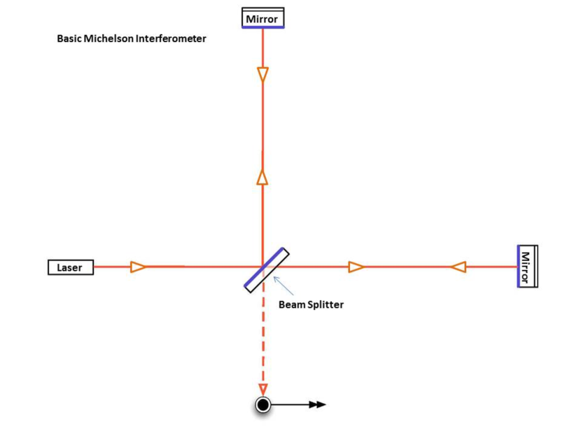
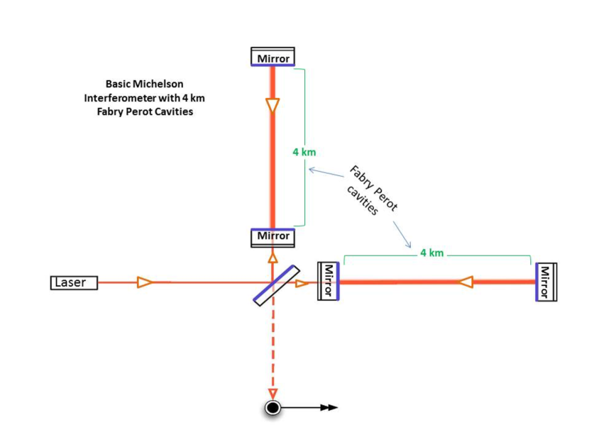
Figure 9: Schematic representation of a Michelson (left) and a Fabry-Perot (right) interferometer (courtesy Caltech/MIT/LIGO Laboratory). In both, the 45-degrees slab represents a beam splitter (which reflects 50% of the photons and lets 50% through) and the photodetector is represented by a dot. The two mirrors close to the beam splitter in the Fabry-Perot design can be thought of as semi-transparent, e.g. a photon will go back and forth many times along each arm before reaching the photodetector. This “Fabry-Perot cavity” thus increases the effective length of the arms (by a factor $\sim 300$ for LIGO). Note that e.g. LISA will instead be a Michelson interferometer.

Let us consider a laser traveling back and forth between two mirrors in free fall.  More precisely, let us assume that the mirrors move along geodesics in a flat spacetime perturbed by a gravitational wave $h^{\mathrm{TT}}_{\mu\nu}$:

$$g_{\mu\nu}=\eta_{\mu\nu}+h^{\mathrm{TT}}_{\mu\nu},$$ (252)

$$\frac{\mathrm{d}^{2}x^{\mu}}{\mathrm{d}\tau^{2}}+\Gamma^{\mu}_{\alpha\beta}\frac{\mathrm{d}x^{\alpha}}{\mathrm{d}\tau}\frac{\mathrm{d}x^{\beta}}{\mathrm{d}\tau}=0\,.$$

Changing variable from the proper time $\tau$ to the coordinate time $t$, one can compute the mirror’s coordinate acceleration as

$$\frac{\mathrm{d}^{2}x^{\mu}}{\mathrm{d}t^{2}}=\frac{\mathrm{d}}{\mathrm{d}t}\Bigg{(}\frac{\mathrm{d}x^{\mu}}{\mathrm{d}\tau}\frac{\mathrm{d}\tau}{\mathrm{d}t}\Bigg{)}=\frac{\mathrm{d}}{\mathrm{d}\tau}\Bigg{[}\frac{\mathrm{d}x^{\mu}}{\mathrm{d}\tau}\left(\frac{\mathrm{d}t}{\mathrm{d}\tau}\right)^{-1}\Bigg{]}\frac{\mathrm{d}\tau}{\mathrm{d}t}=\Bigg{[}\frac{\mathrm{d}^{2}x^{\mu}}{\mathrm{d}\tau^{2}}\left(\frac{\mathrm{d}t}{\mathrm{d}\tau}\right)^{-1}-\left(\frac{\mathrm{d}t}{\mathrm{d}\tau}\right)^{-2}\frac{\mathrm{d}x^{\mu}}{\mathrm{d}\tau}\frac{\mathrm{d}^{2}t}{\mathrm{d}\tau^{2}}\Bigg{]}\frac{\mathrm{d}\tau}{\mathrm{d}t}.$$

Expressing $\frac{\mathrm{d}^{2}x^{\mu}}{\mathrm{d}\tau^{2}}$ and $\frac{\mathrm{d}^{2}t}{\mathrm{d}\tau^{2}}$ by using the geodesic equations, one obtains

$$\frac{\mathrm{d}^{2}x^{\mu}}{\mathrm{d}t^{2}}=-{\Gamma^{\mu}_{\alpha\beta}\dot{x}^{\alpha}\dot{x}^{\beta}}+\dot{x}^{\mu}\Gamma^{0}_{\alpha\beta}\dot{x}^{\alpha}\dot{x}^{\beta}.$$

where the dot denotes $\mathrm{d}/\mathrm{d}t$. Since $\dot{x}^{t}=1$, the spatial acceleration is

$$\frac{\mathrm{d}^{2}x^{i}}{\mathrm{d}t^{2}}=-\left(\Gamma_{tt}^{i}+2\Gamma_{tj}^{i}v^{j}+\Gamma_{jk}^{i}v^{j}v^{k}\right)+v^{i}\left(\Gamma_{tt}^{t}+2\Gamma_{tj}^{t}v^{j}+\Gamma_{jk}^{t}v^{j}v^{k}\right),$$ (253)

where $v^{i}\equiv\dot{x}^{i}$. Assuming that the mirror moves at $v\ll 1$, one finally obtains

$$\frac{\mathrm{d}^{2}x^{i}}{\mathrm{d}t^{2}}\approx-\Gamma_{tt}^{i}.$$ (254)

It is now easy to see that

$$\Gamma_{tt}^{i}=\frac{1}{2}\delta^{ij}\left(2\partial_{t}h_{jt}^{\mathrm{TT}}-\partial_{j}h_{tt}^{\mathrm{TT}}\right)=0,$$ (255)

for a gravitational perturbation in the transverse traceless gauge (c.f. section (II.1)). We have thus reached the apparently paradoxical result that the mirrors do not move under the effect of a passing gravitational wave (if they start at rest).

One must not forget, however, that coordinates (and therefore also the coordinate acceleration) have no physical meaning in GR. What is physically relevant is not the coordinate distance between the free falling mirrors, but their proper distance (which is independent of the coordinates). It is indeed the proper distance that determines the light travel time between mirrors, and thus in turn the phase difference (the laser “fringes”) at the photodetector.

Let us assume for simplicity that the mirrors are on the $x$ axis. Their proper distance is then

$$L^{\rm proper}=\int_{0}^{L}\mathrm{d}x\sqrt{g_{xx}}=\int_{0}^{L}\mathrm{d}x\sqrt{1+h^{\mathrm{TT}}_{xx}}\simeq L\sqrt{1+h_{xx}^{\mathrm{TT}}(t,x=0)}\simeq L\left[1+\frac{1}{2}h_{xx}^{\mathrm{TT}}(t,x=0)\right],$$ (256)

where $L$ is the coordinate distance, and we have assumed not only that the metric perturbation is small, but also that it has wavelength much larger than $L$. (This assumption is needed in the third step.)

The change $\delta L$ in proper distance is therefore

$$\frac{\delta L}{L}\simeq\frac{1}{2}h_{xx}^{\mathrm{TT}}(t,z=0)=\frac{1}{2}h^{\mathrm{TT}}_{ij}u^{i}u^{j}$$ (257)

where in the last step we have introduced the unit-norm vector $u$ to denote the detector’s arm direction. In this way, this equation is valid in a general reference frame.

An alternative (and more instructive) derivation of the same result can be obtained by resorting to the geodesic deviation equation,

$$\frac{\mathrm{D}^{2}v^{\mu}}{\mathrm{d}\tau^{2}}=R^{\mu}_{\alpha\beta\gamma}u^{\alpha}u^{\beta}v^{\gamma}\,,$$ (258)

with $R^{\mu}_{\alpha\beta\gamma}$ the Riemann tensor, $\mathrm{D}/\mathrm{d}\tau$ the covariant derivative along the four velocity, and $v^{\mu}=\delta x^{\mu}$ the separation vector between two neighboring geodesics (the two free falling mirrors). Using FNCs attached to one mirror, one has

$$g_{\mu\nu}=\eta_{\mu\nu}+\mathcal{O}\left(x^{2}/\lambda^{2}\right)\,,$$ (259)

$$u^{\mu}=\delta_{t}^{\mu}+\mathcal{O}\left(x^{2}/\lambda^{2}\right)$$ (260)

where we have used the fact that the mirrors are in free fall ($a^{\mu}=0$) and the curvature radius of the spacetime (Minkowski plus a gravitational wave signal) is given by the signal’s wavelength $\lambda$.

Since the mirrors are at rest in these coordinates, $v^{\mu}=\delta x^{\mu}=(0,L^{i})$. Because the metric is locally flat, $\delta x^{i}=L^{i}$ describes the proper distance between the mirrors, up to corrections of fractional order $\mathcal{O}\left(L^{2}/\lambda^{2}\right)$. From Eq. (258), one then obtains

$$\frac{\mathrm{d}^{2}L^{i}}{\mathrm{d}t^{2}}=-R_{itjt}L^{j}\,.$$ (261)

One can now note that the Riemann tensor of a perturbed Minkowski spacetime is a gauge invariant quantity. This follows simply from the fact that the gauge transformation of a tensor is proportional to the Lie derivative of the background tensor along the gauge generator. Since the Riemann tensor vanishes on the Minkowski background, it follows that it is a gauge invariant quantity at linear order. More explicitly, one can evaluate the Riemann tensor for a perturbed flat spacetime using the results of section (II.3), obtaining

$$R_{itjt}=-\frac{1}{2}\ddot{h}_{ij}^{\mathrm{TT}}+\partial_{i}\partial_{j}\psi+\dot{\Sigma}_{(i,j)}-\frac{1}{2}\ddot{\theta}\delta_{ij}.$$ (262)

in terms of the gauge invariant variables introduced in that section.

Using now Eqs. (58) and (68), it is clear that all the terms in Eq. (262) decay as $1/r^{3}$ (i.e. they correspond to Netwonian and PN tidal forces), and the only term that survives at large distances from a source is the first one. Therefore, one has

$$\frac{\mathrm{d}^{2}L^{i}}{\mathrm{d}t^{2}}=-R_{itjt}L^{j}=\frac{1}{2}\ddot{h}_{ij}^{\mathrm{TT}}L^{j}+\mathcal{O}\left(\frac{1}{r^{3}}\right)\,,$$ (263)

and integrating this equation one obtains Eq. (257). Note that again, we have implicitly made the assumption that the signal’s wavelength is much larger than the distance between the two mirrors, because we have neglected terms $\mathcal{O}\left(x^{2}/\lambda^{2}\right)$ in Eqs. (259)–(260).

The phase difference at the photodetector depends of course on the changes in proper length (i.e. light travel time) induced by the gravitational signal on the first ($\delta L_{1}$) and second ($\delta L_{2}$) arm, i.e. in the low frequency (large wavelength) limit

$$\frac{{\delta L_{1}}-{\delta L_{2}}}{L}=h_{\mathrm{TT}}^{ij}D_{ij}=F_{+}h_{+}+F_{\times}h_{\times}\,,$$ (264)

where

$$D^{ij}=\frac{1}{2}(u^{i}u^{j}-v^{i}v^{j})$$ (265)

(with $u^{i}$ and $v^{i}$ unit vectors in the arm directions) is the detector tensor and $F_{+},F_{\times}$ are the pattern functions (which encode the detector’s response in various directions). The phase difference at the photodetector is then explicitly

$$\Delta\phi=\frac{4\pi\nu}{c}\left({\delta L_{1}}-{\delta L_{2}}\right)=\frac{4\pi\nu L}{c}\left(F_{+}h_{+}+F_{\times}h_{\times}\right)\,,$$ (266)

where $\nu$ is the laser frequency. (Notice the presence of a factor 2 due to the round trip of the laser.)

Exercise 5: Consider an interferometer on the $(x,y)$ plane and a gravitational wave coming from the sky position $\phi,\theta$ (spherical coordinates). Define the wave plus and cross polarizations with respect to two unit vectors $\boldsymbol{e}_{x}$ and $\boldsymbol{e}_{y}$ orthogonal to the propagation direction $\boldsymbol{n}$, and such that the triad $(\boldsymbol{e}_{x},\boldsymbol{e}_{y},\boldsymbol{n})$ is right-handed. Show that the detector’s pattern functions are

$$F_{+}=\frac{1}{2}\cos 2\zeta\left(\cos^{2}\theta+1\right)\cos 2\phi-\sin 2\zeta\cos\theta\sin 2\phi$$

and

$$F_{\times}=\frac{1}{2}\sin 2\zeta\left(\cos^{2}\theta+1\right)\cos 2\phi+\cos 2\zeta\cos\theta\sin 2\phi$$

where $\zeta<\pi/2$ is the angle between $\boldsymbol{e}_{y}$ and the intersection between the plane of the detector and the plane orthogonal to the wave propagation direction.

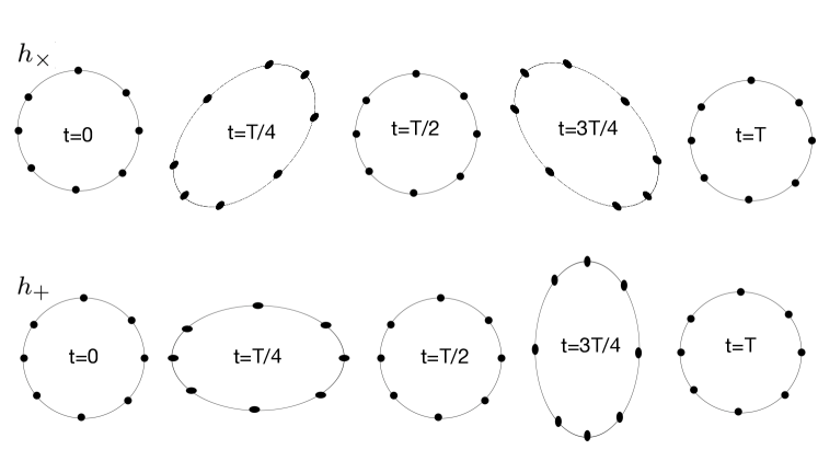
Figure 10: The response of an originally circular ring of particles to a linearly polarized gravitational wave ($h_{+}$ or $h_{\times}$) of period $T$ traveling in the orthogonal direction into the page.

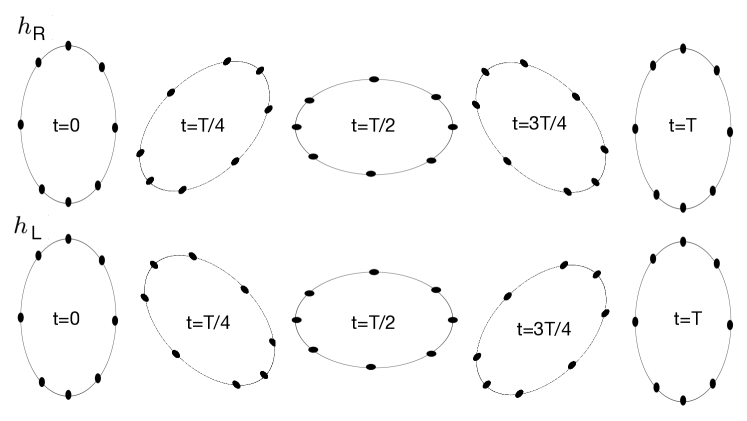
Figure 11: The response of an originally circular ring of particles to a circularly polarized gravitational wave (with right or left helicity) of period $T$ traveling in the orthogonal direction into the page.

VIII.2 A geometric interpretation of the polarizations

Thanks to Eq. (264), we can now provide a geometric interpretation of the two polarizations $h_{+}$ and $h_{\times}$. If one considers a ring of particles on the $(x,y)$ plane and a signal traveling along the $z$-direction, the $h_{+}$ and $h_{\times}$ polarizations deform the ring in a distinct and characteristic way (Fig. (10)). Also shown, in Fig. (11), is the response of a ring to a right-handed or left-handed circularly polarized wave, i.e. one for which the $h_{+}$ and $h_{\times}$ polarizations have a phase difference of $\pm\pi/2$ and the same amplitude. A generic linear polarization corresponds instead to $h_{+}$ and $h_{\times}$ having the same phase (although potentially different amplitudes). Note that from Eq. (184), it follows that for an observer that sees a circular binary face-on ($\iota=0$ or $\iota=\pi$) the signal is circularly polarized; if instead the observer sees the binary edge-on ($\iota=\pi/2$), the polarization is linear. We also notice that additional polarization patterns are present beyond GR eardley . Those arise because the scalar and vector degrees of freedom of Eq. (68) become dynamical (c.f. also section (II.5)).

VIII.3 The response of a gravitational wave detector: the transfer function

Let us now relax the short wavelength assumption ($\lambda\ll L$) that we made when deriving the detector’s response in the previous section. Let us then consider two free falling mirrors in a spacetime with metric

$$g_{\mu\nu}=\eta_{\mu\nu}+h^{\mathrm{TT}}_{\mu\nu},$$ (267)

and integrate null geodesics (the lasers) back and forth between them. As derived in section (VIII.1), the mirrors do not move (with respect to the coordinates) if the perturbation is written in the transverse and traceless gauge.

Let us also make the simplifying assumption that $h_{\mu\nu}^{\mathrm{TT}}$ is given by a plane wave traveling along the $z$-axis:

$$h_{\mu\nu}^{\mathrm{TT}}=\begin{pmatrix}0&0&0&0\\ 0&\cos 2\psi&\sin 2\psi&0\\ 0&\sin 2\psi&-\cos 2\psi&0\\ 0&0&0&0\\ \end{pmatrix}h(t-z)\,.$$ (268)

(Recall that a generic linear perturbation can always be decomposed in a superposition of plane waves.) It is then clear that the spacetime has three Killing vectors

$$k_{1}=\frac{\partial}{\partial x}\,,$$ (269)

$$k_{2}=\frac{\partial}{\partial y}\,,$$ (270)

$$k_{3}=\frac{\partial}{\partial t}+\frac{\partial}{\partial z}\,.$$ (271)

One can then write a tetrad (carried by the mirrors) for the perturbed spacetime as

$$e_{(0)}=\frac{\partial}{\partial t}\,,$$ (272)

$$e_{(1)}=\left(1-\frac{h}{2}\right)\left(\cos\psi\frac{\partial}{\partial x}+\sin\psi\frac{\partial}{\partial y}\right)+\mathcal{O}(h)^{2}\,,$$ (273)

$$e_{(2)}=\left(1+\frac{h}{2}\right)\left(-\sin\psi\frac{\partial}{\partial x}+\cos\psi\frac{\partial}{\partial y}\right)+\mathcal{O}(h)^{2}\,,$$ (274)

$$e_{(3)}=\frac{\partial}{\partial z}\,,$$ (275)

and write the null wave-vector of the laser as

$$\sigma=\nu\left[e_{(0)}+\sin\theta(e_{(1)}\cos\phi+e_{(2)}\sin\phi)+\cos\theta e_{(3)}\right]\,.$$ (276)

Here, $\nu$ is the laser frequency as measured at the mirror, and $\theta$ and $\phi$ describe the laser’s direction. In particular, $\theta$ is the angle between the arm of the detector and the gravitational wave’s propagation direction.

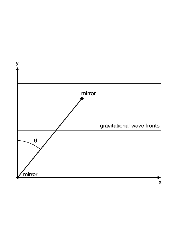
Figure 12: Sketch of the geometry of the system leading to Eq. (287), for $y=0$.

Now, let us recall that the projections of the laser wave-vector on the three Killing vectors are conserved along the laser’s null geodesics:

$$-\sigma\cdot k_{3}=\nu(1-\cos\theta)=\mbox{const}\,,$$ (277)

$$\sigma\cdot k_{1}=\left(1+\frac{h}{2}\right)(\sigma\cdot e_{(1)})\cos\psi-\left(1-\frac{h}{2}\right)(\sigma\cdot e_{(2)})\sin\psi=\mbox{const}\,,$$ (278)

$$\sigma\cdot k_{2}=\left(1+\frac{h}{2}\right)(\sigma\cdot e_{(1)})\sin\psi+\left(1-\frac{h}{2}\right)(\sigma\cdot e_{(2)})\cos\psi=\mbox{const}\,.$$ (279)

This implies also conservation of the combination $\sqrt{(\sigma\cdot k_{1})^{2}+(\sigma\cdot k_{2})^{2}}$, i.e.

$$\sqrt{(\sigma\cdot k_{1})^{2}+(\sigma\cdot k_{2})^{2}}=\left[(1+h)(\sigma\cdot e_{(1)})^{2}+(1-h)(\sigma\cdot e_{(2)})^{2}\right]^{1/2}\approx\nu\sin\theta\left(1+\frac{h}{2}\cos 2\phi\right)=\mbox{const}\,.$$ (280)

Note that this conserved quantity can be rewritten in more compact form as

$$\nu\sin\theta\left(1+\frac{h}{2}\cos 2\phi\right)=\nu\sin\theta\left(1+\frac{Q}{2}\right)=\mbox{const}\,,$$ (281)

$$Q=\frac{h^{\mathrm{TT}}_{ij}n^{i}n^{j}}{1-\cos^{2}\theta}\,,$$ (282)

where $\boldsymbol{n}=\sin\theta\cos(\phi+\psi)\partial_{x}+\sin\theta\sin(\phi+\psi)\partial_{y}+\cos\theta\partial_{z}$ is the detector’s arm direction (from the first to the second mirror) expressed in Cartesian coordinates [this can be obtained by rewriting Eq. (276) using Eqs. (272)–(275) and taking $h\to 0$].

Let us consider now a laser photon starting from first mirror (time “0”), bouncing on the second mirror (time “1”) and returning finally to the first mirror (time “2”). From the conservation laws written above one then obtains

$$\nu_{0}(1-\cos\theta_{0})=\nu_{1}(1-\cos\theta_{1})\,,$$ (283)

$$\nu_{0}\sin\theta_{0}\left(1+\frac{Q_{0}}{2}\right)=\nu_{1}\sin\theta_{1}\left(1+\frac{Q_{1}}{2}\right)\,.$$ (284)

Writing $\cos\theta_{1}=\cos\theta_{0}+\delta\cos\theta+{\cal O}(h)^{2}$, $\sin\theta_{1}=\sin\theta_{0}+\delta\sin\theta+{\cal O}(h)^{2}$ and $\nu_{1}=\nu_{0}+\delta\nu+{\cal O}(h)^{2}$, with $\delta\cos\theta$, $\delta\sin\theta$ and $\delta\nu$ of order ${\cal O}(h)$, one can linearize these equations and obtain

$$\frac{\nu_{1}-\nu_{0}}{\nu_{0}}=\frac{\delta\nu}{\nu_{0}}=\frac{1+\cos\theta_{0}}{2}(Q_{0}-Q_{1})$$ (285)

for the change in laser frequency between the first and second mirror. Performing the same calculation to compute the change in laser frequency when the photon travels in the opposite direction (from the second mirror to the first), one finds

$$\frac{\nu_{2}-\nu_{1}}{\nu_{1}}=\frac{1-\cos\theta_{0}}{2}(Q_{1}-Q_{2})\,.$$ (286)

Note that the different sign of $\cos\theta_{0}$ in Eqs. (286) and (285) appears because during the return trip the photon’s propagation is along $-\boldsymbol{n}$.

Combining these results, one obtains that the change $\Delta\nu$ in laser frequency at the first mirror after a round trip is

$$\frac{\Delta\nu}{\nu}=\frac{\nu_{2}-\nu_{0}}{\nu_{0}}=\frac{1}{2}(1+\cos\theta)Q(t)-\cos\theta\,Q\left(t+\frac{\tau(1-\cos\theta)}{2}\right)-\frac{1}{2}(1-\cos\theta)Q(t+\tau)$$ (287)

where we have dropped the index of the angle $\theta$ since the differences among $\cos\theta_{0}$, $\cos\theta_{1}$ and $\cos\theta_{2}$ appear at higher order, and we have used the fact that $Q_{0}=Q(t)$, $Q_{1}=Q(t+{\tau(1-\cos\theta)}/{2})$ and $Q_{2}=Q(t+\tau)$ with $\tau$ the laser round trip time (c.f. Fig. (12)). From this expression, one can then get the change in the laser phase over a round trip,

$$\Delta\phi=-2\pi\int\Delta\nu\mathrm{d}t\,.$$ (288)

The quantity measured at the photodetector is then the difference between the phase changes $\Delta\phi$ in the first and second arm of the interferometer.

To compute this phase difference and get some physical insight, let us assume for simplicity $\theta={\pi}/{2}$, which yields

$$\Delta\nu=\frac{\nu}{2}[h(t)-h(t+\tau)]\,,$$ (289)

with $h=h_{ij}^{\mathrm{TT}}n^{i}n^{j}$. For a monochromatic wave $h(t)=h_{0}\sin{(2\pi ft)}$ one then has

$$\Delta\phi=-2\pi\int\Delta\nu\mathrm{d}t=\frac{h_{0}\nu}{f}\sin{(f\pi\tau)}\sin{\Big{[}2\pi f\Big{(}t+\frac{\tau}{2}\Big{)}\Big{]}}\,,$$ (290)

which can then be rewritten more simply as

$$\Delta\phi=h\left(t+\frac{\tau}{2}\right)\frac{\nu}{f}\sin{(f\pi\tau)}.$$ (291)

Let us interpret this result in terms of a proper distance change $\delta L$ between the two mirrors, which produces a change in the laser phase (in a round trip) given by

$$\Delta\phi=4\pi\nu\frac{\delta L}{c}\,.$$ (292)

Let us think about this distance change as due to an “effective” strain $h_{\rm eff}$:

$$\frac{\delta L}{L}=\frac{1}{2}h_{\rm eff},$$

where the length can be rewritten in terms of the round trip time $\tau$, $L={\tau c}/{2}$. Replacing in Eq. (292), one then obtains

$$\Delta\phi=\pi\nu\tau h_{\rm eff}\,.$$ (293)

By comparing to Eq. (290), one gets

$$h_{\rm eff}=h\,T(f)\,,$$ (294)

$$T(f)=\frac{\sin{(f\pi\tau})}{f\pi\tau}\,,$$ (295)

where we have introduced the “transfer function” $T(f)$. This calculation can be generalized to more generic propagation directions $\theta\neq\pi/2$.

In summary, we can therefore write the full response of a detector to a Fourier component of frequency $f$ of a gravitational wave signal as

$$\Delta\phi=\frac{4\pi\nu L}{c}\left[F_{+}h_{+}(f)+F_{\times}h_{\times}(f)\right]T(f)\,.$$ (296)

As can be seen from Eq. (295), at low frequencies $T(f)\approx 1$ and this expression reduces to the low frequency response of Eq. (266). At high frequencies $f\gg 1/\tau$, the transfer function instead decays as $1/(f\tau)$, modulated by the oscillations of the numerator of Eq. (295). This explains why the frequency window of gravitational interferometers scales with their armlength $L=c\tau$.

IX Gravitational wave data analysis

As we have seen in the previous section, gravitational wave interferometers measure the interference pattern (i.e. the phase difference) between laser beams traveling between mirrors. The effect of a gravitational signal, however, is generally so small that it is also crucial to adequately understand the statistical error (“noise”) affecting this measurement, and to devise statistical techniques to characterize the signal and its astrophysical source.

IX.1 Gaussian noise and power spectral density

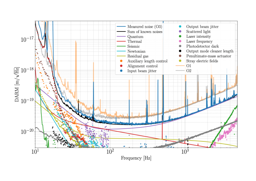
Figure 13: Various contributions to the Advanced LIGO differential armlength (DARM) caused by the noise. This quantity is proportional to the (square root of the) power spectral density. Taken from Ref. ligopsd .

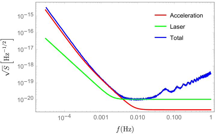
Figure 14: Various contributions to the LISA power spectral density. At high frequencies, one can see the degradation and the oscillations due to the transfer function.

A detector’s output can be written as $s(t)=h(t)+n(t)$, where $h(t)$ is the signal and $n(t)$ is the instrumental noise. Defining the Fourier transform of a time series $A(t)$ as

$$\tilde{A}(f)=\int_{-\infty}^{\infty}A(t)e^{2\pi ift}\mathrm{d}t\,,$$ (297)

the signal is given by $\tilde{h}(f)=\left[F_{+}h_{+}(f)+F_{\times}h_{\times}(f)\right]T(f)$. As for the noise, a common assumption, which turns out to be a good approximation for gravitational wave interferometers, is that of stationarity and Gaussianity.

Stationarity implies that the statistical properties of the noise are time independent. Introducing the ensemble average $\langle\ldots\rangle$, i.e. the average over all possible noise realizations , stationarity implies in particular that $\langle n(t)n(t^{\prime})\rangle$ should only depend on the time difference $\tau=t^{\prime}-t$, i.e. $\langle n(t)n(t^{\prime})\rangle=W(\tau)/2$. (Note also that $\langle n(t)\rangle=0$). Let us see what this implies for the quantity $\langle\tilde{n}^{*}(f)\tilde{n}(f^{\prime})\rangle$. Using the definition of Fourier transform, one has

$$\langle\tilde{n}^{*}(f)\tilde{n}(f^{\prime})\rangle=\int\int\mathrm{d}t\mathrm{d}t^{\prime}\langle n(t)n(t^{\prime})\rangle e^{2\pi i(f^{\prime}t^{\prime}-ft)}$$

$$=\frac{1}{2}\int\int\mathrm{d}t\mathrm{d}\tau W(\tau)e^{2\pi i[(f^{\prime}-f)t+f^{\prime}\tau]}=\frac{1}{2}S(f)\delta(f-f^{\prime})\,,$$ (298)

where $S(f)$ is the Fourier transform of $W(\tau)$ and is known as the (single-sided) power spectral density of the noise. One can also check easily that

$$\langle n(t)^{2}\rangle=\frac{W(0)}{2}=\int_{0}^{\infty}S(f)\mathrm{d}f\,.$$ (299)

The assumption of Gaussian noise then amounts to saying that each Fourier component has a Gaussian probability distribution function, with variance given by Eq. (298). In more detail, because detectors only observe for a finite time $T$ and thus Fourier transforms are implemented as discrete transformations, the frequencies $f_{i}$ at which measurements are performed are spaced by $\Delta f=1/T$. In terms of these discrete frequencies, Eq. (298) becomes

$$\langle\tilde{n}^{*}(f_{i})\tilde{n}(f_{j})\rangle=\frac{1}{2\Delta f}S(f_{i})\delta_{ij}\,,$$ (300)

and the probability $P(n)$ of having a realization $\tilde{n}(f)$ of the noise is

$$P(n)\propto\prod_{i}\exp\left[-\frac{2|\tilde{n}(f_{i})|^{2}\Delta f}{S(f_{i})}\right]=\prod_{i}\exp\left\{-\frac{2\Delta f[(\text{Re}\,\tilde{n}(f_{i}))^{2}+(\text{Im}\,\tilde{n}(f_{i}))^{2}]}{S(f_{i})}\right\}$$

$$\qquad=\exp\left[-2\int_{0}^{\infty}\mathrm{d}f\frac{|\tilde{n}(f)|^{2}}{S(f)}\right]\,.$$ (301)

Here, the index $i$ spans all positive frequencies in the data [since $n(t)$ is real, $\tilde{n}^{*}(f)=\tilde{n}(-f)$ and the signal at negative frequencies follows from that at positive ones].

As can be seen by changing variables in this equation, while the real and imaginary parts of $\tilde{n}(f)$ are Gaussian distributed, the phase of $\tilde{n}(f)$ is uniformly distributed, while the norm $r(f)=|\tilde{n}(f)|$ follows the Rayleigh distribution $p[r(f_{i})]\propto\exp\{-2\Delta f[r(f_{i})]^{2}/S(f_{i})\}r(f_{i})$. Introducing the internal product

$$(A\mid B)\equiv 4\,\text{Re}\int^{\infty}_{0}\frac{\mathrm{d}f\tilde{A}^{*}(f)\tilde{B}(f)}{S(f)},$$ (302)

between two real functions $A(t)$ and $B(t)$, one can rewrite Eq. (301) as

$$P(n)\propto\exp\left[-\frac{1}{2}(n|n)\right]\,.$$ (303)

As we will see, this internal product will also simplify many expressions below.

The behavior of the power spectral density of the noise depends critically on the detector. For ground based interferometers such as LIGO and Virgo, at low frequencies the noise originates chiefly from the laser’s radiation pressure, the seismic noise and the thermal noise of the suspensions; at mid-frequencies the main contributions are the thermal noise from the mirror coatings and the laser noise (radiation pressure and shot noise); at high frequencies the shot noise dominates (see Fig. (13)).

For space-borne detectors like LISA (Fig. (14)), the limitations to the interferometer’s sensitivity come from spurious accelerations of the test masses (due e.g. to cosmic rays, residual gas in the housing, temperature fluctuations) at low frequencies; from the laser shot noise at mid-frequencies; and from the antenna transfer function at high frequencies (c.f. the oscillations in Fig. (14), which are due to the numerator of Eq. (295)).

IX.1.1 Detection in the presence of noise

In order to disentangle the gravitational wave signal from the noise, many techniques have been put forward, among which one of the most popular is match filtering. The latter essentially amounts to cross correlating the detector’s noisy output

$$s(t)=h(t)+n(t)$$ (304)

with a bank of templates $h(t,\boldsymbol{\theta})$. Here, the vector $\boldsymbol{\theta}$ denotes the parameters of the source (i.e. for quasi-circular binaries, the masses, the spins, the distance, the initial phase, the merger time, the inclination, the sky position and the polarization angle). It is quite intuitive that the cross correlation

$$\int\mathrm{d}t\,s(t)h(t,\boldsymbol{\theta})$$ (305)

will “on average” be maximized if the template matches the signal. Taking in fact the average of this equation, one obtains

$$\int\mathrm{d}t\,\langle s(t)h(t,\boldsymbol{\theta})\rangle=\int\mathrm{d}t\,h(t)h(t,\boldsymbol{\theta})\,,$$ (306)

and the second integral is small if the signal and template do not match (because in that case the integrand is highly oscillatory).

Let us try to formalize this statement (see e.g. Ref. maggiore ) by defining a generic filter

$$\hat{A}=\int\mathrm{d}t\,A(t)K(t)$$ (307)

where $A(t)$ is the time series being filters, and $K(t)$ a filter function. Let us try to define a signal-to-noise ratio $S/N$ based on this filter. It is natural to take the signal $S$ as the filter of the detector’s output $s(t)$, averaged over many realizations of the noise:

$$S=\langle\hat{s}\rangle=\int\mathrm{d}t\,\langle s(t)\rangle K(t)=\int\mathrm{d}t\,h(t)K(t)=\int\mathrm{d}f\,\tilde{h}(f)\tilde{K}^{*}(f)\,.$$ (308)

As for the denominator $N$, since $\langle\hat{n}\rangle=0$, we can define instead

$$N^{2} \,=\langle\hat{n}^{2}\rangle=\int\mathrm{d}t\mathrm{d}t^{\prime}\,K(t)K(t^{\prime})\langle n(t)n(t^{\prime})\rangle=\frac{1}{2}\int\mathrm{d}t\mathrm{d}t^{\prime}\,K(t)K(t^{\prime})W(t^{\prime}-t)$$

$$= \quad\frac{1}{2}\int\mathrm{d}t\mathrm{d}t^{\prime}\mathrm{d}f\,K(t)K(t^{\prime})S(f)e^{-2\pi if(t^{\prime}-t)}=\frac{1}{2}\int\mathrm{d}f\,|\tilde{K}(f)|^{2}S(f)\,.$$ (309)

The ratio $S/N$ is then

$$\frac{S}{N}=\frac{\int_{-\infty}^{+\infty}\mathrm{d}f\,\tilde{h}(f)\tilde{K}^{*}(f)}{\left[\int_{-\infty}^{+\infty}\mathrm{d}f(1/2)S(f)|K(f)|^{2}\right]^{1/2}}\,.$$ (310)

By introducing the internal product of Eq. (302), and using the fact that for a real function $A$ one has $\tilde{A}(-f)=\tilde{A}^{*}(f)$, one can rewrite

$$\frac{S}{N}=\frac{(h|u)}{(u|u)^{1/2}}\,,$$ (311)

where we have defined

$$\tilde{u}(f)=\frac{1}{2}S(f)\tilde{K}(f)\,.$$ (312)

Clearly, Eq. (311) is maximized if $u$ and $h$ are parallel, i.e. the filter yielding the optimal signal-to-noise ratio is

$$\tilde{K}(f)\propto\frac{\tilde{h}(f)}{S(f)}\,.$$ (313)

Therefore, if one is searching for a signal, the optimal filter is the template perfectly matching the signal, weighted by the noise power spectral density. This is known as Wiener’s optimal filter theorem. Replacing back into Eq. (311), one obtains that the optimal signal-to-noise ratio is simply given by

$$\left(\frac{S}{N}\right)^{2}={(h|h)}=4\int_{0}^{\infty}\mathrm{d}f\,\frac{|\tilde{h}(f)|^{2}}{S(f)}\,.$$ (314)

IX.2 The signal-to-noise ratio for inspiraling binaries

Equation (314) allows one to compute the optimal signal-to-noise ratio, if the frequency domain signal is known. In the special case of inspiraling binaries, the time domain signal is given, at the lowest PN order, by Eq. (184). The evolution of the gravitational wave frequency $f_{\rm gw}$ is instead described by Eq. (189), which yields

$$f_{\rm gw}=\frac{1}{\pi}M_{c}^{-5/8}\left(\frac{5}{256(t_{c}-t)}\right)^{3/8}\,,$$ (315)

where we have identified the integration constant $t_{c}$ with the the coalescence time. This identification is justified because it yields a frequency diverging at $t=t_{c}$. This divergence is not physical, but simply signals that the quadrupole formula, used to derive Eq. (189), breaks down. It is natural to assume that this breakdown happens at the merger, since the assumption of a binary system, implicit in the quadrupole formula, ceases to apply there.

As we have seen in section (VIII), the detector is sensitive to a linear combination of $h_{+}$ and $h_{\times}$, modulated by the transfer function. Neglecting for the moment the transfer function – because its effect is small for LIGO/Virgo, while for LISA it is usually included in the power spectral density of the noise (c.f. Fig. (14)) – we can write the detector’s response, using Eq. (184), as

$$h(t)=F_{+}h_{+}+F_{\times}h_{\times}=\frac{4M_{c}^{5/3}[\pi f_{\rm gw}(t)]^{2/3}}{D}\left[F_{+}\frac{1+\cos^{2}\iota}{2}\cos\Phi(t)+\cos\iota F_{\times}\sin\Phi(t)\right]\,$$ (316)

where $\Phi(t)=\int_{t_{0}}^{t}\mathrm{d}t^{\prime}2\pi f_{\rm gw}(t^{\prime})$.

Note that although we derived Eq. (316) in flat space, it is possible to show (see e.g. Ref. maggiore ) that it is valid also in a Robertson-Walker spacetime, provided that the frequency $f_{\rm gw}$ is the one measured at the detector [where it is redshifted by a factor $1/(1+z)$ relative to the frequency at the source], the masses are redshifted, i.e. $M_{c}\to M_{c}(1+z)$, and $D$ is interpreted as the luminosity distance $D_{L}$.

To perform the Fourier transform analytically, one can use the stationary phase approximation. Considering first the $h_{+}$ polarization, let us rewrite Eq. (316) as

$$h(t)=\frac{A(t)}{2}\left[e^{i\Phi(t)}+e^{-i\Phi(t)}\right]$$ (317)

by introducing an amplitude $A(t)$, the Fourier transform is

$$\tilde{h}(f)=\int\mathrm{d}t\,\frac{A(t)}{2}e^{2\pi ift}\left[e^{i\Phi(t)}+e^{-i\Phi(t)}\right]\,.$$ (318)

The main contribution to this integral comes from the regions the phase does not change rapidly (the contribution of the other regions is negligible because the fast oscillations average to zero). Note that we are only interested in computing $\tilde{h}(f)$ for $f>0$ since $\tilde{h}(-f)=\tilde{h}^{*}(f)$ [because $h(t)$ is real]. Then, because $\dot{\Phi}=f_{\rm gw}>0$, the first term in square brackets in Eq. (318) has no stationary points, and we can thus neglect it. As for the second term, let us denote by $t_{*}$ the time at which the phase is stationary, i.e. $\dot{\Phi}(t_{*})=2\pi f$. Taylor expanding near this stationary point, one obtains

$$\tilde{h}(f)\approx\frac{1}{2}A(t_{*})e^{i[2\pi ft_{*}-\Phi(t_{*})]}\int\mathrm{d}t\,e^{-i\ddot{\Phi}(t_{*})(t-t_{*})^{2}/2}=\frac{1}{2}A(t_{*})e^{i[2\pi ft_{*}-\Phi(t_{*})]}\sqrt{\frac{2}{\ddot{\Phi}(t_{*})}}\int_{-\infty}^{\infty}\mathrm{d}x\,e^{-i\,x^{2}}$$

$$\qquad=\frac{1}{2}A(t_{*})e^{i[2\pi ft_{*}-\Phi(t_{*})-\pi/4]}\sqrt{\frac{2\pi}{\ddot{\Phi}(t_{*})}}\,.$$ (319)

One can then express $t_{*}$ as a function of $f$ by solving $f=\dot{\Phi}(t_{*})/(2\pi)=f_{\rm gw}(t_{*})$. Using Eq. (315) one then has

$$t_{c}-t_{*}=\frac{5}{256}M_{c}^{-5/3}(\pi f)^{-8/3}\,,$$ (320)

which can be used into Eq. (319) to obtain the amplitude and phase as functions of frequency. Doing the same calculation for $h_{\times}$ yields the same result, but with an additional factor $i$ (i.e. a $\pi/2$ phase difference). The final result then reads

$$\tilde{h}(f)=\frac{1}{D_{L}}\left(\frac{5}{24}\right)^{1/2}\pi^{-2/3}M_{c}^{5/6}f^{-7/6}Qe^{i\psi}\,,$$ (321)

$$\psi=2\pi ft_{*}-\Phi(t_{*})-\pi/4$$ (322)

with $t_{*}$ given by Eq. (320) and

$$Q=F_{+}\frac{1+\cos^{2}\iota}{2}+i\cos\iota F_{\times}\,.$$ (323)

Note that we have expressed this final result in terms of $D_{L}$, and thus $f$ and $M_{c}$ must be interpreted as the detector-frame frequency and the redshifted chirp mass, respectively.

One can then compute the signal-to-noise ratio using Eq. (314) as

$$\left(\frac{S}{N}\right)^{2}=\frac{5}{6}\frac{1}{\pi^{4/3}}\frac{1}{D_{L}^{2}}\left(\frac{GM_{c}}{c^{3}}\right)^{5/3}|Q|^{2}\int_{0}^{f_{\rm max}}df\frac{f^{-7/3}}{S(f)}\,,$$ (324)

where for clarity we have reinstated $G$ and $c$. The factor $Q$ depends on the sky position and orientation of the source (c.f. Eq. (323)). For sources with optimal sky position and inclination ($\iota=\theta=0$) one has $Q=1$, while an average over sky position and inclination (assuming isotropic distributions) yields $\langle Q^{2}\rangle=4/25$. Signal-to-noise ratios allowing detection are typically $S/N\gtrsim 8$.

Exercise 6: Using the stationary phase approximation, show that the signal-to-noise ratio of a quasi-monochromatic signal

$$h(t)=F_{+}h_{+}(t)+F_{\times}h_{\times}(t)\equiv\sqrt{2}A\cos\left[2\pi\left(f_{0}+\frac{\dot{f_{0}}t}{2}\right)t+\phi_{0}\right]$$ (325)

is given by

$$\left(\frac{S}{N}\right)^{2}=\frac{2A^{2}T}{S(f_{0})}\,,$$ (326)

where $T$ is the observation time. [Hint: the maximum integration frequency depends on the observation time.]

IX.3 Parameter estimation

Let us now suppose that a gravitational wave signal has been detected in the data $s$, and let us examine whether the parameters $\boldsymbol{\theta}$ of the source can be inferred. In principle, the probability distribution function for the parameters conditional on the data, i.e. the “posterior distribution” $P(\boldsymbol{\theta}|s)$, is given by Bayes theorem in terms of the likelihood $P(s|\boldsymbol{\theta})$ and the “prior distribution” $P(\boldsymbol{\theta})$:

$$P(\boldsymbol{\theta}|s)\propto P(s|\boldsymbol{\theta})P(\boldsymbol{\theta})\,.$$ (327)

Here, the prior distribution encodes the knowledge on the parameters before data are taken (e.g. it can be taken to be uniform if one wants to remain agnostic). As for the likelihood, i.e. the probability to obtain the data $s$ given the waveform parameters $\boldsymbol{\theta}$, it can be computed from Eq. (303) by replacing $n=s-h$ as per Eq. (304):

$$P(s|\boldsymbol{\theta})\propto\exp\left[-\frac{1}{2}(s-h_{\boldsymbol{\theta}}|s-h_{\boldsymbol{\theta}})\right]\propto\exp\left[-\frac{1}{2}(h_{\boldsymbol{\theta}}|h_{\boldsymbol{\theta}})+(h_{\boldsymbol{\theta}}|s)\right]\,,$$ (328)

where $h_{\boldsymbol{\theta}}$ is the template.

Given the large dimensionality of the parameter space (up to 15 parameters for quasi-circular binaries), the posteriors predicted by Eq. (327) cannot be plotted or sampled by brute force. A more sophisticated approach based on Markov-Chain-Monte-Carlo or nested sampling techniques is needed, which is outside the scope of these simple notes. It is possible, however, to expand the posteriors around their maximum in a Taylor series, obtaining the Fisher matrix of the system. In more detail, let consider the case of uninformative (uniform) priors, $P(\boldsymbol{\theta})=$  const, and assume that the posterior distribution peaks at $\boldsymbol{\theta}=\boldsymbol{\bar{\theta}}$. Imposing $\partial P(s|\boldsymbol{\theta})/\partial\theta^{i}=0$ at the peak, one then gets

$$\left(\frac{\partial h_{\boldsymbol{\theta}}}{\partial\theta^{i}}(\boldsymbol{\bar{\theta}})\Bigg{|}s\right)-\left(\frac{\partial h_{\boldsymbol{\theta}}}{\partial\theta^{i}}(\boldsymbol{\bar{\theta}})\Bigg{|}h_{\boldsymbol{\theta}}(\boldsymbol{\bar{\theta}})\right)=0\,.$$ (329)

Expanding now the posterior distribution at quadratic order near the peak and assuming a high signal-to-noise ratio [which allows for approximating $s\approx h_{\boldsymbol{\theta}}({\boldsymbol{\bar{\theta}}}$)], one obtains

$$P(\boldsymbol{\theta}|s)\propto\exp\left[-\frac{1}{2}\Gamma_{ij}(\theta^{i}-\bar{\theta}^{i})(\theta^{j}-\bar{\theta}^{j})\right]\,,$$ (330)

where we have introduced the Fisher matrix

$$\Gamma_{ij}=\left(\frac{\partial h_{\boldsymbol{\theta}}}{\partial\theta^{i}}(\boldsymbol{\bar{\theta}})\Bigg{|}\frac{\partial h_{\boldsymbol{\theta}}}{\partial\theta^{j}}(\boldsymbol{\bar{\theta}})\right)\,.$$ (331)

In the high signal-to-noise ratio limit, the posterior distribution near the peak is therefore described by a multivariate Gaussian with covariance matrix

$$C_{ij}=(\Gamma^{-1})_{ij}\,.$$ (332)

While not useful to analyze real data, the Fisher matrix formalism can be used to obtain predictions about how well the parameters are measurable by a given detector. This information is encoded in the covariance matrix. Note that eliminating the row and column corresponding to a parameter in the covariance matrix amounts to marginalizing over that parameter. Instead, eliminating the row and column corresponding to a parameter in the Fisher matrix corresponds to assuming that parameter is known exactly.

Exercise 7: Consider a quasicircular system of two black holes with masses $m_{1,2}$ of $30$ and $35M_{\odot}$ at 400 Mpc luminosity distance. Compute the signal-to-noise ratio for a detector with power spectral density

$$S=10^{-49}[x^{-4.14}-5x^{-2}+111(1-x^{2}+x^{4}/2)/(1+x^{2}/2)]{\rm Hz}^{-1},$$

with $x=f/(215\,{\rm Hz})$, tapering the inspiral waveform of Eq. (321) at the ISCO of a particle with mass $\mu=m_{1}m_{2}/(m_{1}+m_{2})$ around a Schwarzschild black hole of mass $M=m_{1}+m_{2}$. Assume optimal inclination and sky position, and no spins.

Exercise 8: For the quasi-monochromatic signal of Exercise 6, assume $f_{0}=80$ Hz, $\dot{f}_{0}$ from Eq. (189) and compute the amplitude $A$ that gives $S/N=20$ for an observation time of one year and the detector of Exercise 7. For such a source, compute the covariance matrix of the parameters ($A$, $f_{0}$ and $\dot{f}_{0}$).

References

- (1) B. P. Abbott et al. [LIGO Scientific and Virgo], “Observation of Gravitational Waves from a Binary Black Hole Merger,” Phys. Rev. Lett. 116, no.6, 061102 (2016) doi:10.1103/PhysRevLett.116.061102 [arXiv:1602.03837 [gr-qc]].
- (2) M. J. Pfenning and E. Poisson, Phys. Rev. D 65, 084001 (2002) doi:10.1103/PhysRevD.65.084001 [arXiv:gr-qc/0012057 [gr-qc]].
- (3) E. E. Flanagan and S. A. Hughes, New J. Phys. 7, 204 (2005) doi:10.1088/1367-2630/7/1/204 [arXiv:gr-qc/0501041 [gr-qc]].
- (4) V. F. Mukhanov, H. A. Feldman and R. H. Brandenberger, Phys. Rept. 215, 203-333 (1992) doi:10.1016/0370-1573(92)90044-Z
- (5) J. M. Bardeen, Phys. Rev. D 22, 1882-1905 (1980) doi:10.1103/PhysRevD.22.1882
- (6) E. Barausse and L. Lehner, “Post-Newtonian approach to black hole-fluid systems,” Phys. Rev. D 88, no.2, 024029 (2013) doi:10.1103/PhysRevD.88.024029
- (7) C. M. Will, “Theory and Experiment in Gravitational Physics,” Cambridge University Press, 2018
- (8) E. Poisson and C. M. Will, “Gravity: Newtonian, Post-Newtonian, Relativistic”, Cambridge U. Press, 2014
- (9) M. Bonetti and E. Barausse, “Post-Newtonian constraints on Lorentz-violating gravity theories with a MOND phenomenology,” Phys. Rev. D 91, 084053 (2015) [erratum: Phys. Rev. D 93, 029901 (2016)] doi:10.1103/PhysRevD.91.084053 [arXiv:1502.05554 [gr-qc]].
- (10) M. Bonetti, E. Barausse, G. Faye, F. Haardt and A. Sesana, “About gravitational-wave generation by a three-body system,” Class. Quant. Grav. 34, no.21, 215004 (2017) doi:10.1088/1361-6382/aa8da5 [arXiv:1707.04902 [gr-qc]].
- (11) E. Poisson, “A Relativist’s Toolkit: The Mathematics of Black-Hole Mechanics,” Cambridge University Press, 2009, doi:10.1017/CBO9780511606601
- (12) F. de Felice and C. J. S. Clarke, Cambridge University Press, 1992, ISBN 978-0-521-42908-5, 978-0-521-26639-0
- (13) E. Bertschinger, “Stress-Energy Pseudotensors and Gravitational Radiation Power”, http://web.mit.edu/edbert/GR/gr7.pdf
- (14) C. W. Misner, K. S. Thorne and J. A. Wheeler, “Gravitation,” W. H. Freeman, 1973, ISBN 978-0-7167-0344-0, 978-0-691-17779-3
- (15) S. L. Shapiro and S. A. Teukolsky, “Black holes, white dwarfs, and neutron stars: The physics of compact objects,”, 1983, doi:10.1002/9783527617661
- (16) R. M. Wald, “General Relativity,” Chicago Univ. Pr., 1984, doi:10.7208/chicago/9780226870373.001.0001
- (17) P. K. Townsend, “Black holes: Lecture notes,” [arXiv:gr-qc/9707012 [gr-qc]].
- (18) J. H. Taylor, L. A. Fowler and P. M. McCulloch, “Measurements of general relativistic effects in the binary pulsar PSR 1913+16,” Nature 277, 437-440 (1979) doi:10.1038/277437a0
- (19) A. Buonanno and T. Damour, Phys. Rev. D 59, 084006 (1999) doi:10.1103/PhysRevD.59.084006 [arXiv:gr-qc/9811091 [gr-qc]].
- (20) K. Akiyama et al. [Event Horizon Telescope], “First M87 Event Horizon Telescope Results. I. The Shadow of the Supermassive Black Hole,” Astrophys. J. Lett. 875, L1 (2019) doi:10.3847/2041-8213/ab0ec7 [arXiv:1906.11238 [astro-ph.GA]].
- (21) J. M. Bardeen, W. H. Press and S. A. Teukolsky, “Rotating black holes: Locally nonrotating frames, energy extraction, and scalar synchrotron radiation,” Astrophys. J. 178, 347 (1972) doi:10.1086/151796
- (22) S. Babak, A. Taracchini and A. Buonanno, Phys. Rev. D 95, no.2, 024010 (2017) doi:10.1103/PhysRevD.95.024010 [arXiv:1607.05661 [gr-qc]].
- (23) A. Le Tiec, E. Barausse and A. Buonanno, Phys. Rev. Lett. 108, 131103 (2012) doi:10.1103/PhysRevLett.108.131103 [arXiv:1111.5609 [gr-qc]].
- (24) K. S. Thorne, “Disk accretion onto a black hole. 2. Evolution of the hole.,” Astrophys. J. 191, 507-520 (1974) doi:10.1086/152991
- (25) E. Barausse, V. Morozova and L. Rezzolla, “On the mass radiated by coalescing black-hole binaries,” Astrophys. J. 758, 63 (2012) doi:10.1088/0004-637X/758/1/63 [arXiv:1206.3803 [gr-qc]].
- (26) M. Campanelli, C. O. Lousto and Y. Zlochower, “Spinning-black-hole binaries: The orbital hang up,” Phys. Rev. D 74, 041501 (2006) doi:10.1103/PhysRevD.74.041501 [arXiv:gr-qc/0604012 [gr-qc]].
- (27) E. Berti, V. Cardoso and A. O. Starinets, “Quasinormal modes of black holes and black branes,” Class. Quant. Grav. 26, 163001 (2009) doi:10.1088/0264-9381/26/16/163001 [arXiv:0905.2975 [gr-qc]].
- (28) T. Regge and J. A. Wheeler, “Stability of a Schwarzschild singularity,” Phys. Rev. 108, 1063-1069 (1957) doi:10.1103/PhysRev.108.1063
- (29) F. J. Zerilli, “Effective potential for even parity Regge-Wheeler gravitational perturbation equations,” Phys. Rev. Lett. 24, 737-738 (1970) doi:10.1103/PhysRevLett.24.737
- (30) V. Ferrari and B. Mashhoon, “New approach to the quasinormal modes of a black hole,” Phys. Rev. D 30, 295-304 (1984) doi:10.1103/PhysRevD.30.295
- (31) B. F. Schutz and C. M. Will, “Black hole normal modes: a semianalytic approach,” Astrophys. J. Lett. 291, L33-L36 (1985) doi:10.1086/184453
- (32) D. R. Brill, P. L. Chrzanowski, C. Martin Pereira, E. D. Fackerell and J. R. Ipser, “Solution of the scalar wave equation in a kerr background by separation of variables,” Phys. Rev. D 5, 1913-1915 (1972) doi:10.1103/PhysRevD.5.1913
- (33) S. A. Teukolsky, “Perturbations of a rotating black hole. 1. Fundamental equations for gravitational electromagnetic and neutrino field perturbations,” Astrophys. J. 185, 635-647 (1973) doi:10.1086/152444
- (34) S. L. Detweiler, “Black holes and gravitational waves. III - The resonant frequencies of rotating holes,” Astrophys. J. 239, 292-295 (1980) doi:10.1086/158109
- (35) J. Weber, “Gravitational Radiation,” Phys. Rev. Lett. 18, no.13, 498-501 (1967) doi:10.1103/PhysRevLett.18.498
- (36) D. M. Eardley, D. L. Lee, A. P. Lightman, R. V. Wagoner and C. M. Will, “Gravitational-wave observations as a tool for testing relativistic gravity,” Phys. Rev. Lett. 30, 884-886 (1973), doi:10.1103/PhysRevLett.30.884
- (37) A. Buikema et al., “Sensitivity and performance of the Advanced LIGO detectors in the third observing run”, Phys. Rev. D 102, 062003 (2020), doi:10.1103/PhysRevD.102.062003
- (38) M. Maggiore, “Gravitational Waves. Vol. 1: Theory and Experiments,” Oxford University Press, 2007, ISBN 978-0-19-857074-5, 978-0-19-852074-0