Efficiently Explaining CSPs with Unsatisfiable
Subset Optimization

Abstract

We build on a recently proposed method for stepwise explaining the solutions to Constraint Satisfaction Problems (CSPs) in a human understandable way. An explanation here is a sequence of simple inference steps where simplicity is quantified by a cost function. Explanation generation algorithms rely on extracting Minimal Unsatisfiable Subsets (MUSs) of a derived unsatisfiable formula, exploiting a one-to-one correspondence between so-called non-redundant explanations and MUSs. However, MUS extraction algorithms do not guarantee subset minimality or optimality with respect to a given cost function. Therefore, we build on these formal foundations and address the main points of improvement, namely how to generate explanations efficiently that are provably optimal (with respect to the given cost metric). To this end, we developed (1) a hitting set-based algorithm for finding the optimal constrained unsatisfiable subsets; (2) a method for reusing relevant information across multiple algorithm calls; and (3) methods for exploiting domain-specific information to speed up the generation of explanation sequences. We have experimentally validated our algorithms on a large number of CSP problems. We found that our algorithms outperform the MUS approach in terms of explanation quality and computational time (on average up to 56 % faster than a standard MUS approach).

1 Introduction

Building on old ideas to explain domain-specific propagation performed by constraint solvers (?, ?), we recently introduced a method that takes as input a satisfiable set of constraints and explains the solution finding process in a human understandable way (?). Explanations in this work are sequences of simple inference steps that involve as few constraints and previously derived facts as possible. Each explanation step derives at least one new fact implied by a combination of constraints and previously derived facts.

The explanation steps of ? (?) are heuristically optimised with respect to a given cost function that should approximate human understandability, e.g. taking into account the number of constraints and facts considered, as well as an estimate of their cognitive complexity. For example, when evaluating explanations for logic grid puzzles, the given clues of the puzzle are considered more difficult than simpler reasoning tricks, that are present in all instances of such puzzles and therefore have a higher cost.

In practice, the explanation generation algorithms presented in ? (?) rely heavily on calls to Minimal Unsatisfiable Subsets (MUS) (?) of a derived unsatisfiable formula, exploiting a one-to-one correspondence between so-called non-redundant explanations and MUSs.

However, the algorithm of ? (?) has two main weaknesses. First, it provides no guarantees on the quality of the generated explanations due to internally relying on the computation of $\subseteq$-minimal unsatisfiable subsets, which are often suboptimal with respect to the given cost function. Second, it suffers from performance problems: the lack of optimality is partly overcome by calling a MUS algorithm on increasingly larger subsets of constraints for each candidate fact to explain. However, using multiple MUS calls per literal in each iteration quickly leads to efficiency problems, causing the explanation generation process to take several hours, even for simple puzzles designed to be solvable by humans.

Contributions

In this paper, we tackle the limitations discussed above. We develop algorithms that aid explaining in Constraint Satisfaction Problems and improve the state of the-art in the following ways:

• We develop algorithms that compute (cost-)Optimal Unsatisfiable Subsets (from now on called OUSs) based on the well-known hitting-set duality which is also used to compute cardinality-minimal MUSs (?, ?).

• We observe that in the explanation setting, many of the individual calls for MUSs (or OUSs) can actually be replaced by a single call that searches for an optimal unsatisfiable subset among subsets satisfying certain structural constraints. We formalize and generalize this observation by introducing the Optimal Constrained Unsatisfiable Subsets (OCUS) problem. We then show how $O(n^{2})$ calls to MUS/OUS can be replaced by $O(n)$ calls to an OCUS oracle, where $n$ denotes the number of facts to explain.

• We develop techniques for further optimizing the O(C)US algorithms, exploiting domain-specific information coming from the fact that we are in the explanation-generation context. Such optimizations include (i) the development of methods for information re-use between consecutive O(C)US calls; as well as (ii) an explanation-specific version of the OCUS algorithm.

• Finally, we extensively evaluate our approaches on a large number of CSP problems.

Paper Structure

The rest of this paper is structured as follows. In Section 2, we discuss work related to efficiently computing unsatisfiable subsets. Section 3 introduces the theoretical foundations of our implicit hitting set approach. Section 4 motivates our work, and Section 5 introduces the OCUS problem and a hitting set-based algorithm for computing OCUSs. Then, in Section 6, we look at 2 other methods for computing the next best explanation in the explanation sequence. In Section 7 we present methods to improve the efficiency of our algorithms, e.g. by making them incremental or by using different methods to extract multiple correction subsets. Finally, in Section 8 we evaluate our approach on a large set of puzzle instances and conclude with some future perspectives.

Publication History

This article is an extension of a previous paper presented at the International Joint Conference on Artificial Intelligence 2021 (?). The current paper extends the previous paper with more detailed examples, extensive experiments on a large data set of puzzles, as well as the novel Explain-One-Step-OCUS-Split algorithm for efficiently computing explanations.

2 Related Work

In the last few years, driven by the increasing many successes in Artificial Intelligence (AI), there has been a growing need for eXplainable Artificial Intelligence (XAI) (?). In the research community, this need manifests itself through the emergence of (interdisciplinary) workshops and conferences on this topic (?, ?), as well as American and European incentives to stimulate research in the area (?, ?, ?).

While the main focus of XAI research has been on explaining black-box machine learning systems (?, ?, ?). Model-based systems, which are typically considered more transparent, are also in need of explanation mechanisms. For instance, ? (?) surveys the important methods that use argumentation (?) to provide explainability in AI, with for example applications in medical diagnosis (?). Abstract argumentation frameworks introduce an abstract formalism to explain argumentative acceptance (?, ?, ?). Description Logics (?) on the other hand, aim at explaining logical proofs (?, ?), i.e ‘why does phi follow from psi?’.

The main focus of our work lies in providing explainable agency (?) to Constraint Programming (CP) (?) and Boolean Satisfiability (SAT) (?) systems. Advances in solving, as well as hardware improvements, allow for such systems now easily consider millions of alternatives in short amounts of time. Because of this complexity, the question arises of how to generate human-interpretable explanations of the conclusions they make. Explanations have seen a rejuvenation in various subdomains of constraint reasoning (?, ?, ?, ?). In the CP and SAT communities, there has been a strong focus on explaining unsatisfiable problem instances (?), for example by extracting a minimal unsatisfiable subset (MUS) from the problem constraints (?).

We have recently introduced step-wise explanations (?) to explain the solution of satisfiable instances, exploiting a one-to-one correspondence between so-called non-redundant explanations and MUSs of a derived program. The focus of ? (?) was on explaining Zebra puzzles; building on this work, ? (?) investigated interpretable explanations using MUSs for a wide range of puzzles. Our current work is motivated by a concrete algorithmic need: to generate these explanations efficiently, we need algorithms that can find MUSs that are optimal with respect to a given cost function, where the cost function approximates human-understandability of the corresponding explanation step.

The closest related work can be found in the literature on generating or enumerating MUSs (?, ?, ?, ?). Various techniques are used to find MUSs, including manipulation of resolution proofs produced by SAT solvers (?, ?, ?), incremental solving to enable/disable clauses and branch-and-bound search (?), BDD-manipulation methods (?). Some methods rely on seed-shrink algorithms (?, ?) which repeatedly start from unsatisfiable seed (an unsatisfiable core) and shrink the seed to a MUS. Other methods work by means of translation into a so-called Quantified MaxSAT (?), a field that combines the expressiveness of Quantified Boolean Formulas (QBF) (?) with techniques from Maximum Satisfiability (MaxSAT) (?), or by exploiting the so-called hitting set duality (?). To the best of our knowledge, only few works have considered optimizing MUSs: the only criterion considered so far is cardinality-minimality (?, ?).

An abstract framework for describing hitting set–based algorithms, including optimization, has been developed by ? (?). While our approach can be seen to fit within the framework, the terminology is focused on MaxSAT rather than MUS and would complicate our exposition.

3 Background

In this section, we introduce the terminology and concepts related to explanation generation. We present all methods using propositional logic but our results easily generalize to richer languages, such as constraint languages, as long as the semantics is given in terms of a satisfaction relation between expressions in the language and possible states of affairs (assignments of values to variables).

Let $\Sigma$ be a set of propositional symbols, also called atoms; this set is implicit in the rest of the paper. A literal is an atom $p$ or its negation $\lnot p$. A clause is a disjunction of literals, i.e. $c_{1}=x_{1}\vee\lnot x_{2}$. A formula $\mathcal{F}$ in conjunctive normal form (CNF) is a conjunction of clauses. Slightly abusing notation, a clause is also viewed as a set of literals and a formula as a set of clauses.

A (partial) interpretation $\mathcal{I}$ is a consistent (not containing both $p$ and $\lnot p$) set of literals. Satisfaction of a formula $\mathcal{F}$ by an interpretation is defined as usual (?): an interpretation $\mathcal{I}$ satisfies $\mathcal{F}$ if $\mathcal{I}$ contains at least one literal from each clause in $\mathcal{F}$. A model of $\mathcal{F}$ is an interpretation that satisfies $\mathcal{F}$; $\mathcal{F}$ is said to be unsatisfiable if it has no models. An interpretation that satisfies $\mathcal{F}$ is also called a model of $\mathcal{F}$. A formula $\mathcal{F}$ is satisfiable if it has at least one model and unsatisfiable otherwise.

A literal $l$ is a consequence of a formula $\mathcal{F}$ if $l$ holds in all $\mathcal{F}$’s models. The maximal consequence of a formula $\mathcal{F}$, denotes a consequence that holds in all models. If $I$ is a set of literals, we write $\mathbf{\overline{\raisebox{0.0pt}[1.1pt]{{I}}}}$ for the set of negated literals $\{\lnot\ell\mid\ell\in I\}$.

Example 1.

Let $\mathcal{C}_{1}$ be the CNF formula over atoms $x_{1},x_{2},x_{3}$ with the following four clauses:

$$c_{1}:=\lnot x_{1}\vee\lnot x_{2}\vee x_{3}\qquad c_{2}:=\lnot x_{1}\vee x_{2}\vee x_{3}\qquad c_{3}:=x_{1}\qquad c_{4}:=\lnot x_{2}\vee\lnot x_{3}$$

An example of an interpretation is $\{\lnot x_{2},x_{3}\}$. The maximal consequence of formula $\mathcal{C}$ is $\{x_{1},\lnot x_{2},x_{3}\}$.

In the following, we introduce key properties on unsatisfiable subsets on which we build our algorithms.

Definition 1.

A Minimal Unsatisfiable Subset (MUS) of $\mathcal{F}$ is an unsatisfiable subset $\mathcal{S}$ of $\mathcal{F}$ for which every strict subset of $\mathcal{S}$ is satisfiable. $\mathit{MUSs}(\mathcal{F})$ denotes the set of MUSs of $\mathcal{F}$.

Definition 2.

A set $\mathcal{S}\subseteq\mathcal{F}$ is a Maximal Satisfiable Subset (MSS) of $\mathcal{F}$ if $\mathcal{S}$ is satisfiable and for all $\mathcal{S}^{\prime}$ with $\mathcal{S}\subsetneq\mathcal{S}^{\prime}\subseteq\mathcal{F}$, $\mathcal{S}^{\prime}$ is unsatisfiable.

Definition 3.

A set $\mathcal{S}\subseteq\mathcal{F}$ is a correction subset of $\mathcal{F}$ if $\mathcal{F}\setminus\mathcal{S}$ is satisfiable. Such a $\mathcal{S}$ is a minimal correction subset (MCS) of $\mathcal{F}$ if no strict subset of $\mathcal{S}$ is also a correction subset. $\mathit{MCSs}(\mathcal{F})$ denotes the set of minimal correction subsets of $\mathcal{F}$.

Each MCS of $\mathcal{F}$ is the complement of an MSS of $\mathcal{F}$ and vice versa.

Definition 4.

Given a collection of sets $\mathcal{H}$, a hitting set of $\mathcal{H}$ is a set $h$ such that $h\cap C\neq\emptyset$ for every $C\in\mathcal{H}$. A hitting set is minimal if no strict subset of it is also a hitting set.

The next proposition is the well-known hitting set duality (?, ?) between MCSs and MUSs that forms the basis of our algorithms, as well as algorithms to compute MSSs (?) and cardinality-minimal MUSs (?).

Proposition 1.

A set $\mathcal{S}\subseteq\mathcal{F}$ is an MCS of $\mathcal{F}$ iff it is a minimal hitting set of $\mathit{MUSs}(\mathcal{F})$. A set $\mathcal{S}\subseteq\mathcal{F}$ is a MUS of $\mathcal{F}$ iff it is a minimal hitting set of $\mathit{MCSs}(\mathcal{F})$.

Consider the following examples to illustrate the concepts related to unsatisfiability introduced in the previous definitions:

Example 2.

Let $\mathcal{C}_{2}$ be the unsatisfiable CNF formula over atoms $x_{1},x_{2},x_{3}$ with the following clauses:

$$c_{1}:=\lnot x_{1}\vee\lnot x_{2}\vee x_{3}\qquad c_{2}:=\lnot x_{1}\vee x_{2}\vee x_{3}\qquad c_{3}:=\lnot x_{2}\vee\lnot x_{3}\qquad c_{4}:=x_{1}$$

$$c_{5}:=\lnot x_{1}\vee x_{2}\qquad c_{6}:=\lnot x_{1}\vee\lnot x_{3}$$

In Example 2, the subset of clauses $\{c_{1},c_{2},c_{4},c_{6}\}$ is an example of a Minimal Unsatisfiable Subset (MUS) and $\{\underline{c_{1}}\},\{\underline{c_{4}}\},\{\underline{c_{2}},c_{5}\},\{c_{5},\underline{c_{6}}\},\{c_{3},\underline{c_{6}}\}$ are examples of minimal correction subsets (MCSs). We observe that MUS $\{c_{1},c_{2},c_{4},c_{6}\}$ hits at least one clause of each MCS.

4 Motivation

Our work is motivated by the problem of explaining the solution to constraint satisfaction problems, or how to explain the information entailed from it, through a sequence of simple explanation steps. This can be used to teach people problem solving skills; to search for mistakes in the problem formulation that lead to undesired models; to compare the difficulty of related satisfaction problems (through the number and complexity of steps required) and in systems that provide interactive tutoring.

4.1 Step-wise Explanation Generation

Our original explanation generation algorithm (?), shown in Algorithm 1, starts from a formula $\mathcal{C}$ (in the application it comes from a high-level CSP), an initial interpretation $I_{0}$ (here also seen as a conjunction of literals) and a cost function $f$ which quantifies the difficulty of an explanation step, e.g. by means of a weight for each clause.

An explanation step is an implication $I^{\prime}\wedge\mathcal{C}^{\prime}\implies N$ where

• $I^{\prime}$ is a subset of already derived literals I;

• $\mathcal{C}^{\prime}$ is a subset of the constraints of the input formula $\mathcal{C}$; and

• $N$ is a set of literals entailed by $I^{\prime}$ and $\mathcal{C}^{\prime}$ which are not yet explained.

The goal is to find a sequence of simple explanation steps that explain the maximal consequence $I_{\mathit{end}}$, also referred to as the end interpretation, entailed by the given initial interpretation $I_{0}$ (line 1). In each explanation step, some literals from $I_{\mathit{end}}$ are explained, resulting in a precision-increasing sequence of interpretations $I_{0}\preceq I_{1}\preceq\dots I_{end}$. Therefore, the intermediate interpretation $I$ at a given step in this sequence will consist of all the literals “derived so far” and the remaining literals to be explained will explain correspond to $I_{\mathit{end}}\setminus I$.

1 $I_{\mathit{end}}\leftarrow\mathtt{propagate}(I\wedge\mathcal{C})$

2 Seq $\leftarrow$ empty sequence

3 $I\leftarrow I_{0}$

4 while $I\neq Iend$ do

5       $S\leftarrow\texttt{Explain-One-Step}(\mathcal{C},f,I,I_{\mathit{end}})$

6       $I^{\prime}\leftarrow I\cap S$

7       $\mathcal{C}^{\prime}\leftarrow C\cap S$

8       $N\leftarrow\mathtt{propagate}(I^{\prime}\wedge\mathcal{C}^{\prime})$

9       append $(I^{\prime},\mathcal{C}^{\prime},N)$ to Seq

10       $I\leftarrow I\cup N$

11      

12 end while

13return Seq

14

Algorithm 1 $\mathtt{explain}(\mathcal{C},f,I_{0})$

The subset returned by Explain-One-Step (line 1 of Algorithm 1) is then mapped back to the set of derived literals $I^{\prime}$ (line 1) and constraints $C^{\prime}$ (line 1). Finally, at line 1, we propagate the used literals $I^{\prime}$ and constraints $C^{\prime}$ present in the found subset to derive new information $N^{\prime}$ that holds at the intersection of all models of $I^{\prime}\wedge C^{\prime}$, i.e., we compute the maximal consequence of $I^{\prime}\wedge C^{\prime}$.

Example 3.

Let $C$ be the CNF formula over atoms $x_{1},x_{2},x_{3}$ with the following four clauses:

$$c_{1}:=\lnot x_{1}\vee\lnot x_{2}\vee x_{3}\qquad c_{2}:=\lnot x_{1}\vee x_{2}\vee x_{3}\qquad c_{3}:=x_{1}\qquad c_{4}:=\lnot x_{2}\vee\lnot x_{3}$$

Let $I=\{\lnot x_{2}\}$ be the given interpretation with corresponding maximal consequence $I_{\mathit{end}}=\{x_{1},\lnot x_{2},x_{3}\}$. $I_{\mathit{end}}\setminus I=\{x_{1},x_{3}\}$ represents the set of remaining literals to explain and its negation is denoted by $\overline{I_{\mathit{end}}\setminus I}=\{\lnot x_{1},\lnot x_{3}\}$. An example of an explanation step is

$$\lnot x_{2}\wedge c_{2}\wedge c_{3}\implies x_{3}$$

where we use derived literal $\lnot x_{2}$ and constraints $c_{2}$ and $c_{3}$ to infer $x_{3}$.

Note that all explanations in the examples are expressed in terms of this logical representation, however, the explanations can be translated back to the original input (e.g. natural language clues,, alldifferent constraints, …).

4.2 Explanation Step

The key part of Explain-One-Step is the search for the best explanation step given an interpretation $I$ of the literals derived so far. The procedure depicted in Algorithm 2 shows the gist of how this is done. It takes as input the problem constraints $\mathcal{C}$, a cost function $f$ quantifying the quality of explanations, an interpretation $I$ containing all literals derived so far in the sequence, and the interpretation to be explained $I_{\mathit{end}}$.

To compute an explanation step, this procedure iterates over the literals to be explained (line 2 of Algorithm 2), computes for each of them an associated MUS (line 2), and then selects the lowest cost one from the found MUSs (line 2). The reason this works is a one-to-one correspondence between MUSs of $\mathcal{C}\land I\land\neg\ell$ and so-called non-redundant explanation of $\ell$ in terms of (subsets of) $\mathcal{C}$ and $I$ (?).

1 ${\cal S}_{best}\leftarrow\mathit{nil}$

2 for $\ell\in\{I_{\mathit{end}}\setminus I\}$ do

3       ${\cal S}\leftarrow\texttt{MUS}{(\mathcal{C}\land I\land\neg\ell)}$

4       if $f({\cal S})<f({\cal S}_{best})$ then

5             ${\cal S}_{best}\leftarrow{\cal S}$

6            

7       end if

8      

9 end for

10return ${\cal S}_{best}$

11

Algorithm 2 $\texttt{Explain-One-Step}(\mathcal{C},f,I,I_{\mathit{end}})$

Example 4 (Example 3 continued).

For computing a non-redundant explanation of $x_{3}$ zith given interpretation $I=\{\lnot x_{2}\}$, we simply extract a

$$MUS(\mathcal{C}\land I\land\neg\ell)=MUS(\mathcal{C}\wedge\{\lnot x_{2}\}\wedge\{\lnot x_{3}\})=\{c_{2},c_{3},\{\lnot x_{2}\},\{\lnot x_{3}\}\}$$

also written as $\lnot x_{2}\wedge c_{2}\wedge c_{3}\implies x_{3}$.

Throughout the paper, we consider cost functions $f$ that map a subset $\mathcal{S}\subseteq\mathcal{C}\wedge I_{\mathit{end}}\wedge\overline{I_{\mathit{end}}\setminus I}$ to a numerical value $f(\mathcal{S})$, namely, a weighted sum on the constraints present in the subset $\mathcal{S}$. $\overline{I_{\mathit{end}}\setminus I}$ refers to the negation of the remaining literals to explain $\{\lnot\ell\mid\ell\in I_{\mathit{end}}\setminus I\}$ introduced to compute non-redundant explanation steps with MUSs.

4.3 Concluding Remarks

Experiments have shown that such a MUS-based approach can easily take hours, especially when, at every explanation step, repeated MUS calls are performed for each remaining literal to explain (lines 2-2 of Algorithm 2) to increase the chance of finding a low-cost MUS. Furthermore, MUS extraction algorithms do not guarantee of $\subseteq$-minimality or optimality with respect to a given cost function $f$. Therefore, in ? (?), we handle the absence of $\subseteq$-minimality and optimality guarantees by heuristically considering increasingly larger subsets of the unsatisfiable formula ($\mathcal{C}\land I\land\neg l$).

Hence, there is a need for algorithmic improvements to make it more practical. We see three main points of improvement, all of which are addressed by our generic OCUS algorithm presented in the next section.

• First, since the algorithm is based on MUS calls, there is no guarantee that the explanation found is indeed optimal (with respect to the given cost function). Performing multiple MUS calls is only a heuristic used to circumvent the restriction that there are no algorithms for cost-based unsatisfiable subset optimization.

• Second, this algorithm uses MUS calls for every literal $\ell\in I_{\mathit{end}}\setminus I$ to explain separately. The goal of all these calls is to find a single unsatisfiable subset of $\mathcal{C}\land I\land\overline{(I_{\mathit{end}}\setminus I)}$ that contains exactly one literal from $\overline{(I_{\mathit{end}}\setminus I)}=\{\lnot\ell\mid\ell\in I_{\mathit{end}}\setminus I\}$. This raises the question of whether it is possible to compute a single (optimal) unsatisfiable subset subject to constraints, where in our case, the constraint is to include exactly one literal from $\overline{(I_{\mathit{end}}\setminus I)}$.

• Third, the algorithm that computes an entire explanation sequence makes use of repeated calls to Explain-One-Step, and will therefore solve many similar problems. This raises the question of incrementality: can we reuse the computed data structures to achieve speedups in later calls?

In the next section, we introduce the concept of Optimal Constrained Unsatisfiable Subsets to address the first two main points of improvement. We address the third point in Section 7 along with other optimizations to speed up the generation of explanation sequence.

5 Optimal Constrained Unsatisfiable Subsets

In this section, we address the first two challenges highlighted at the end of Section 4.3, namely (1) the lack of optimality guarantees when relying on MUS extraction methods (and heuristics) to compute an explanation step, and (2) whereas the optimal explanation of a single literal can be formalized as an optimal MUS (with respect to a given objective), finding the optimal next explanation step over all literals remains an open question. To tackle these, we introduce the concept of an Optimal Constrained Unsatisfiable Subset (OCUS) and propose an algorithm for computing one.

Definition 5.

Let $\mathcal{F}$ be a formula, $f:2^{\mathcal{F}}\to\mathbb{N}$ a cost function and $p$ a predicate $p:2^{\mathcal{F}}\to\{\mathit{true},\mathit{false}\}$. We call $\mathcal{S}\subseteq\mathcal{F}$ an Optimal Constrained Unsatisfiable Subset (OCUS) of $\mathcal{F}$ (with respect to $f$ and $p$) if

• $\mathcal{S}$ is unsatisfiable,

• $p(\mathcal{S})$ is true

• all other unsatisfiable $\mathcal{S}^{\prime}\subseteq\mathcal{F}$ for which $p(\mathcal{S}^{\prime})$ is true satisfy $f(\mathcal{S}^{\prime})\geq f(\mathcal{S})$.

Proposition 2.

Let $\mathcal{F}$ be a CNF formula, ${p}$ be a predicate specified as a CNF over (meta)-variables indicating the inclusion of clauses of $\mathcal{F}$, and ${f}$ be a cost-function obtained by assigning a weight to each such meta-variable, then the problem complexity of finding an OCUS is $\Sigma^{\emph{P}}_{2}$-complete.

Proof.

If we assume that the predicate $p$ is specified itself as a CNF over (meta)-variables indicating the inclusion of clauses of $\mathcal{F}$, and $f$ is obtained by assigning a weight to each such meta-variable, then the complexity of the problem of finding an OCUS is the same as that of the SMUS (cardinality-minimal or ‘Smallest’ MUS) problem (?): the associated decision problem is $\Sigma^{P}_{2}$-complete. Hardness follows from the fact that SMUS is a special case of OCUS; containment follows - intuitively - from the fact that this can be encoded as an $\exists\forall$-QBF using a Boolean circuit encoding of the costs. ∎

In the next sections, we first explain how OCUS can be used to compute an explanation step and then propose an algorithm for computing OCUSs using the well-known hitting set duality between MUSs and MCSs (?, ?).

5.1 Explain-One-Step with OCUS

Explain-One-Step implicitly uses an “exactly one of” constraint on the set of literals to explain $\{\ell\in I_{\mathit{end}}\setminus I\}$, and the way this is done is by considering each literal $\ell$ from that set separately. It searches for a good, but not necessarily optimal CUS (an Unsatisfiable Subset that satisfies the Constraint in question). However, the goal is to find an optimal one. Therefore, when considering the procedure Explain-One-Step from the perspective of OCUS defined above, the task of the procedure is to compute an OCUS of the formula $\mathcal{F}:=\mathcal{C}\land I\land\overline{I_{\mathit{end}}\setminus I}$ where $p$ is the predicate that holds for subsets containing exactly one literal of $\overline{I_{\mathit{end}}\setminus I}$. The pseudocode for this is shown in Algorithm 3.

1

2 $\mathcal{F}\leftarrow\mathcal{C}\land I\land\overline{I_{\mathit{end}}\setminus I}$

3 $p\leftarrow(S\mapsto\#(S\cap\overline{I_{\mathit{end}}\setminus I})=1)$

4 $\mathcal{S},\mathit{status}\leftarrow\texttt{OCUS}(\mathcal{F},f,p)$

5 if $\mathit{status}\neq\mathit{FAILURE}$ then return $\mathcal{S}$

6 else return $\emptyset$

Algorithm 3 $\texttt{Explain-One-Step-OCUS}(\mathcal{C},f,I,I_{\mathit{end}})$

Explaining 1 Literal per Step.

We define the ‘exactly one’ constraint $p$ as the equality constraint shown on line 3 of Algorithm 3. $p$ evaluates to true if the size of the intersection of the negated literals to explain $I_{\mathit{end}}\setminus I$ with the subset $\mathcal{S}$ of $\mathcal{F}$ considered is equal to 1, otherwise $p$ evaluates to false.

The call to OCUS on line 3 of Explain-One-Step-OCUS will never lead to the $\mathit{FAILURE}$ case, since an OCUS is guaranteed to exist for the input cost function $f$, predicate $p$ and formula $\mathcal{F}$ we are considering. Failure may occur for a different predicate $p$. For example, consider the predicate $p:(\mathcal{S}\mapsto f(S)\leq v)$ of Algorithm 5, which evaluates to true if a subset $\mathcal{S}$ has a value less than a given bound $v$. In this case it can lead to failure if no OCUS exists for a given bound $v$.

In the next section, we provide the details on how to compute an OCUS on line 3.

5.2 Computing an OCUS

In order to compute an OCUS of a given formula, we propose to build on the hitting set duality of Proposition 1. For this, we will assume to have access to a solver CondOptHittingSet that can compute hitting sets of a given collection of sets that are optimal (w.r.t. a given cost function $f$) among all hitting sets satisfying a condition $p$. The choice of the underlying hitting set solver will thus determine which types of cost functions and constraints are possible.

In our implementation, we use a cost function $f$ which is encoded as a linear term (weighted sum), where e.g. constraints are given a larger weight than already derived literals. For example, (unit) clauses representing previously derived facts can be given small weights, and regular clauses can be given large weights, so that explanations are penalized for including clauses when previously derived facts can be used instead. Condition $p$ can be easily encoded as a linear constraint (see Eq. 8 for an example), thus allowing the use of highly optimized mixed integer programming (MIP) solvers to compute optimal hitting sets. In the following, we explain how the conditional optimal hitting set problem CondOptHittingSet can be encoded into MIP to reason over combinations of clauses and literals (hitting sets) of the unsatisfiable formula.

Hitting Set Problem

Given $\mathcal{F}$, we define a MIP decision variable $d_{c}$ for every clause $c\in\mathcal{F}$, and write ${D}=\{d_{c}\mid c\in\mathcal{F}\}$ for the set of all such variables. We assume a given collection of sets-to-hit $\mathcal{H}$. The goal is to find a hitting set $h\subseteq D$ that hits every set-to-hit at least once (Eq. 3), satisfies predicate $p$ (Eq. 2), and minimizes $f(D)$ (Eq. 1). The CondOptHittingSet formulation is as follows:

$$\small\operatorname*{minimize}_{{h\subseteq{D}}}\quad f(h)$$ (1)

$$s.t.\quad p(h)$$ (2)

$$\sum_{c\in H}{d}_{c}\geq 1,\quad \forall H\in\mathcal{H}$$ (3)

$${d}_{c}\in\{0,1\},\quad \forall{d}_{c}\in{D}$$ (4)

In the case of OCUS, every set-to-hit corresponds to a correction subset of $\mathcal{F}$.

OCUS Algorithm

Our generic algorithm for computing OCUSs is depicted in Algorithm 4. It combines the hitting set-based approach for MUSs of ? (?) with the use of a MIP solver for (weighted) hitting sets as proposed for maximum satisfiability by ? (?). The key novelty is the ability to add structural constraints to the hitting set solver, without impacting the duality principles of Proposition 1, as we will show.

1 $\mathcal{H}\leftarrow\emptyset$

2 while true do

3       $\mathcal{S},\mathit{status}\leftarrow\texttt{CondOptHittingSet}(\mathcal{H},f,p)$

4       if $\mathit{status}=\mathit{FAILURE}$ then return $(\emptyset,\mathit{status})$

5      

6      if  $\lnot\texttt{{SAT}}(\mathcal{S})$  then

7             return $(\mathcal{S},\mathit{status})$

8            

9       end if

10      $\mathcal{K}\leftarrow\texttt{CorrSubsets}(\mathcal{S},\mathcal{F})$

11       $\mathcal{H}\leftarrow\mathcal{H}\cup\mathcal{K}$

12      

13 end while

Algorithm 4 $\texttt{OCUS}(\mathcal{F},f,p)$

The algorithm alternates calls to a hitting set solver with calls to a SAT oracle on a subset $\mathcal{S}$ of $\mathcal{F}$. In case the SAT oracle returns true, i.e., subset $\mathcal{S}$ is satisfiable, $\mathcal{K}$ a set of subsets of $F\setminus S$ is returned by CorrSubsets and added to the collection of sets-to-hit $\mathcal{H}$.

Smallest MUS of ? (?)

The key differences with the SMUS algorithm are the calls to a CondOptHittingSet solver (resp. MinimumHS) and the CorrSubsets (resp. grow) procedure. In the SMUS algorithm, the purpose of grow is to expand a satisfiable subset $\mathcal{S}$ of $\mathcal{F}$ further such that its complement, a correction subset, is as small as possible. Shrinking the correction subset as a result of grow finds stronger constraints on the sets-to-hit, since it restricts the choice of clauses to be selected.

In our algorithm we make use of the CorrSubsets procedure which returns a non-empty set of correction subsets. In the case of OCUS, the calls for hitting sets will also take into account the cost ($f$), and the meta-level constraints ($p$). As such, It is not clear a priori which properties a good CorrSubsets function should have here. In Section 5.3, we propose different domain-specific methods for enumerating multiple correction subsets.

For the correctness of the algorithm, all we need to know is that for a given satisfiable subset $\mathcal{S}$, CorrSubsets returns a non-empty set of correction subsets $\mathcal{K}$, where $\forall\ \mathcal{C}\in\mathcal{K}:\mathcal{C}\subseteq(F\setminus S)$. At any given step, if $\mathcal{S}$ is satisfiable, $\mathcal{H}$ is guaranteed to grow, since a non-empty set of correction subsets $\mathcal{K}$ is returned that is disjoint from $\mathcal{S}$. Therefore $\mathcal{K}$ cannot be present in $\mathcal{H}$. The completeness and soundness of the algorithm follow from the fact that the algorithm is guaranteed to terminate since there is a countable number of correction subsets of $\mathcal{F}$, and from Theorem 6, which states that what is returned is indeed a solution and that a solution will be found if it exists.

Theorem 6.

Let $\mathcal{H}$ be a set of correction subsets of $\mathcal{F}$. If $\mathcal{S}$ is a hitting set of $\mathcal{H}$ that is $f$-optimal among the hitting sets of $\mathcal{H}$ that satisfy a predicate $p$, and $\mathcal{S}$ is unsatisfiable, then $\mathcal{S}$ is an OCUS of $\mathcal{F}$. If $\mathcal{H}$ has no hitting sets satisfying $p$, then $\mathcal{F}$ has no OCUSs.

Proof.

For the first claim, it is clear that $\mathcal{S}$ is unsatisfiable and satisfies $p$. Hence all we need to show is the $f$-optimality of $\mathcal{S}$. If there would exist some other unsatisfiable subset $\mathcal{S}^{\prime}$ that satisfies $p$ with $f(\mathcal{S}^{\prime})\leq f(\mathcal{S})$, we know that $\mathcal{S}^{\prime}$ would hit every minimal correction set of $\mathcal{F}$, and hence also every set in $\mathcal{H}$ (since every correction set is the superset of a minimal correction set). Since $\mathcal{S}$ is $f$-optimal among hitting sets of $\mathcal{H}$ that satisfy $p$, and since $\mathcal{S}^{\prime}$ also hits $\mathcal{H}$ and satisfies $p$, it must be that $f(\mathcal{S})=f(\mathcal{S}^{\prime})$.

The second claim follows immediately from Proposition 1 and the fact that an OCUS is an unsatisfiable subset of $\mathcal{F}$. ∎

Perhaps surprisingly, the correctness of the proposed algorithm does not depend on the monotonicity properties of $f$ nor $p$. In principle, any (computable) cost function and condition on the unsatisfiable subsets can be used. In practice, however, one is bound by the limitations of the chosen hitting set solver.

As an illustration, we provide an example of one call to Explain-One-Step-OCUS (Algorithm 3) and the corresponding OCUS-call in detail (Algorithm 4) for our running example:

Example 5 (continued).

Recall the 4 previously introduced clauses from our running example $C:=c_{1}\wedge c_{2}\wedge c_{3}\wedge c_{4}$ with:

$$c_{1}:=\lnot x_{1}\vee\lnot x_{2}\vee x_{3}\qquad c_{2}:=\lnot x_{1}\vee x_{2}\vee x_{3}\qquad c_{3}:=x_{1}\qquad c_{4}:=\lnot x_{2}\vee\lnot x_{3}$$

Consider a call to Explain-One-Step-OCUS with $I=\emptyset$ and $I_{\mathit{end}}=\{x_{1},\lnot x_{2},x_{3}\}$. We add the following three new clauses, which represent the complement of the literals to be derived $\overline{I_{\mathit{end}}\setminus I}$:

$$\{\lnot x_{1}\}\qquad\{x_{2}\}\qquad\{\lnot x_{3}\}$$

The cost function $f$ is defined as a linear sum

$$f(\mathcal{S})=\sum_{c\in\mathcal{S}}w_{i}\cdot c_{i}$$ (5)

over the following clause weights:

Clause weights: $$\ w_{c_{1}}=60\ \qquad w_{c_{2}}=60\qquad\ \ \ w_{c_{3}}=100\qquad w_{c_{4}}=100$$

$$I\wedge\overline{I_{\mathit{end}}\setminus I} \ w_{\lnot x_{1}}=1\qquad w_{x_{2}}=1\ \ \ \qquad w_{\lnot x_{3}}=1$$ weights:

We encode the same cost function in the MIP encoding as a weighted sum using the corresponding decision variables as follows:

$$f(\mathcal{S})=\sum_{c\in\mathcal{S}}w_{c}\cdot d_{c}$$ (6)

To ensure that we only explain one literal at a time, we add predicate $p$ as

$$p(S):=\#(S\cap\{\lnot x_{1},x_{2},\lnot x_{3}\})=1$$ (7)

The MIP encoding of the predicate $p$ corresponds to

$$p(h):=\sum_{c\in\overline{I_{\mathit{end}}\setminus I}}d_{c}={d}_{\{\lnot x_{1}\}}+{d}_{\{x_{2}\}}+{d}_{\{\lnot x_{3}\}}=1$$ (8)

At Algorithm 3 of Explain-One-Step-OCUS, $\mathcal{F}$ is constructed, consisting of :

$$\mathcal{F}=C\land I\land\overline{(I_{\mathit{end}}\setminus I)}=c_{1}\wedge\dots\wedge c_{4}\wedge\lnot x_{1}\wedge x_{2}\wedge\lnot x_{3}$$ (9)

Finally, to generate an explanation step, we call OCUS on formula $\mathcal{F}$ with the given cost function $f$ and exactly-one constraint $p$:

$$\texttt{OCUS}(\mathcal{F},f,p)$$ (10)

In this small example, the $\texttt{CorrSubsets}(\mathcal{S},\mathcal{F})$ procedure simply returns $\{F\setminus S\}$.

Step $\mathcal{S}$ $\texttt{{SAT}}(\mathcal{S})$ $\mathcal{H}\leftarrow\mathcal{H}\cup\texttt{CorrSubsets}(\mathcal{S},\mathcal{F})$ $\emptyset$ 1. $\{\lnot x_{3}\}$ $\mathit{true}$ $\{\{c_{1},c_{2},c_{3},c_{4},\lnot x_{1},x_{2}\}\}$ 2. $\{\lnot x_{1}\}$ $\mathit{true}$ $\{\dots,\{c_{1},c_{2},c_{3},c_{4},x_{2},\lnot x_{3}\}\}$ 3. $\{x_{2}\}$ $\mathit{true}$ $\{\dots,\{c_{1},c_{2},c_{3},c_{4},\lnot x_{1},\lnot x_{3}\}\}$ 4. $\{c_{1},x_{2}\}$ $\mathit{true}$ $\{\dots,\{c_{2},c_{3},c_{4},\lnot x_{1},\lnot x_{3}\}\}$ 5. $\{c_{2},x_{2}\}$ $\mathit{true}$ $\{\dots,\{c_{1},c_{3},c_{4},\lnot x_{1},\lnot x_{3}\}\}$ 6. $\{c_{1},\lnot x_{3}\}$ $\mathit{true}$ $\{\dots,\{c_{2},c_{3},c_{4},\lnot x_{1},x_{2}\}\}$ 7. $\{c_{2},\lnot x_{1}\}$ $\mathit{true}$ $\{\dots,\{c_{1},c_{3},c_{4},x_{2},\lnot x_{3}\}\}$ 8. $\{c_{1},\lnot x_{1}\}$ $\mathit{true}$ $\{\dots,\{c_{2},c_{3},c_{4},x_{2},\lnot x_{3}\}\}$ 9. $\{c_{2},\lnot x_{3}\}$ $\mathit{true}$ $\{\dots,\{c_{1},c_{3},c_{4},\lnot x_{1},x_{2}\}\}$ 10. $\{c_{4},x_{2}\}$ $\mathit{true}$ $\{\dots,\{c_{1},c_{2},c_{3},\lnot x_{1},\lnot x_{3}\}\}$ 11. $\{c_{3},x_{2}\}$ $\mathit{true}$ $\{\dots,\{c_{1},c_{2},c_{4},\lnot x_{1},\lnot x_{3}\}\}$ 12. $\mathbf{\{c_{3},\lnot x_{1}\}}$ $\mathit{false}$

Table 1: Example 5 - Intermediate steps when computing an OCUS for Explain-One-Step-OCUS where $\texttt{CorrSubsets}(\mathcal{S},\mathcal{F})=\{\mathcal{F}\setminus\mathcal{S}\}$.

Table 1 breaks down the intermediate steps of algorithm 4 for generating an OCUS of given $\mathcal{F}$, $f$ and $p$. First, the collection of sets-to-hit $\mathcal{H}$ is initialized as the empty set. At each iteration, the hitting set solver searches for a cost-minimal assignment that hits all sets in $\mathcal{H}$ and that contains exactly one of $\{\lnot x_{1},x_{2},\lnot x_{3}\}$ (due to $p$). If the hitting set is unsatisfiable, it is guaranteed to be an OCUS.

The first iterations show that the OCUS algorithm first hits all the literals of $\overline{I_{\mathit{end}}\setminus I}$ (steps 1-3 of Table 1) and then starts combining one literal of $\overline{I_{\mathit{end}}\setminus I}$ with the remaining clauses until an OCUS is found (step 12). Finally, step 12 of Table 1 signifies that using clause $c_{3}$ we can derive $x_{1}$, and more formally $c_{3}\implies x_{1}$.

Incremental MIP Solver

The OCUS algorithm requires repeatedly computing hitting sets over an increasing collection of sets-to-hit. Initializing the MIP solver once and keeping it warm throughout the OCUS iterations allows it to reuse information from previous solver calls to solve the current hitting set problem. Similar to ? (?), we notice a speed-up between 3 to 5 times by keeping the solver warm compared to initializing a new MIP solver instance at every iteration.

As can be seen in Table 1, the OCUS algorithm requires many intermediate steps to find an OCUS. Note, for example, that the computed correction subsets contain more than 1 literal to explain that are not relevant for explaining the literal in the current hitting set. Taking step 2 as an example, if $\{\lnot x_{1}\}$ is a hitting set, its corresponding correction subset $\{c_{1},c_{2},c_{3},c_{4},x_{2},\lnot x_{3}\}$ contains $\{x_{2},\lnot x_{3}\}$ which cannot be taken.

Even though our running example has a rather small number of clauses, OCUS needs to combine an increasingly large number of literals and clauses to find an OCUS. Next, we investigate how to efficiently grow a given satisfiable subset in order to reduce the size of the corresponding correction subset. By imposing stronger restrictions on the hitting sets, we will be able to reduce the number of sets to hit.

5.3 Computing Correction Subsets

The CorrSubsets procedure generates a set of correction subsets starting from a given satisfiable subset $\mathcal{S}$ of an unsatisfiable formula $\mathcal{F}$. However, calling Explain-One-Step-OCUS on our running example has shown that a naive ‘No grow’:

$$\texttt{CorrSubsets}(\mathcal{S},\mathcal{F})\leftarrow\{\mathcal{F}\setminus\mathcal{S}\}$$ (11)

drastically increases the number of sets-to-hit required compared to using the model provided by the SAT solver. This last observation suggests that the satisfiable subset $\mathcal{S}$ should be efficiently grown into a larger satisfiable subset before computing the complement:

$$\texttt{CorrSubsets}(\mathcal{S},\mathcal{F})\leftarrow\{\mathcal{F}\setminus\texttt{Grow}(\mathcal{S},\mathcal{F})\}$$ (12)

5.3.1 Growing satisfiable subsets using domain-specific information

The goal of the Grow phase of the CorrSubsets procedure (see Eq. 12) is to turn $\mathcal{S}$ into a larger satisfiable subformula of $\mathcal{F}$. The effect of this is that the complement added to $\mathcal{H}$ will be smaller, and hence imposes stronger restrictions on the hitting sets.

There are multiple conflicting criteria that determine what makes an effective ‘grow’ procedure. On the one hand, we want our subformula to be as large as possible (which would ultimately correspond to computing a maximal satisfiable subformula), but on the other hand, we also want the procedure to be very efficient, as it is called in every iteration.

In the case of explanations, we make the following observations:

• Our formula at hand (using the notation from the Explain-One-Step-OCUS algorithm) consists of three types of clauses: (1) (translations of) the problem constraints (this is $\mathcal{C}$) (2) literals representing the assignment found (this is $I$), and (3) the negations of literals not yet derived (this is $\overline{I_{\mathit{end}}\setminus I}$).

• $\mathcal{C}$ and $I$ together are satisfiable, with assignment $I_{end}$, and mutually supportive, by this we mean that making more clauses in $\mathcal{C}$ true, more literals in $I$ will automatically become true and vice versa.

• The constraint $p$ enforces that each hitting set will contain exactly one literal of $\overline{I_{\mathit{end}}\setminus I}$

Since the restrictions on the third type of elements of $\mathcal{F}$ are already strong, it makes sense to search for a maximal satisfiable subset of $\mathcal{C}\cup I$ with hard constraints that $\mathcal{S}$ should be satisfied, using a call to an efficient (partial) MaxSAT solver.

Furthermore, we can initialize this call as well as any call to a SAT solver with the polarities for all variables set to the value they take in $I_{\mathit{end}}$.

We evaluate different grow strategies as part of the $\texttt{CorrSubsets}(\mathcal{S},\mathcal{F})$ procedure in the experiments section including:

SAT

extracts a satisfying model from the SAT solver to turn $\mathcal{S}$ into a larger satisfiable subset. This grow will be considered the baseline for comparing the other grow-variants.

SubsetMax-SAT

extends the satisfiable subset computed by SAT by looping over every remaining clause $c\in\mathcal{F}\setminus\mathcal{S}$. If $\mathcal{S}\cup\{c\}$ is satisfiable, then clause $c$ is added to $\mathcal{S}$ as well as any other clause from $c^{\prime}\in\mathcal{F}\setminus\mathcal{S}\cup\{c\}$ that is satisfied in the model found by the SAT solver.

Dom.-spec. MaxSAT

grows a satisfiable subset $\mathcal{S}$ with a MaxSAT solver using only the previously derived facts and the original constraints.

MaxSAT Full

grows satisfiable subset $\mathcal{S}$ with a MaxSAT solver using the full unsatisfiable formula $\mathcal{F}$.

In the experiments, we omit the ‘No grow’ procedure where the complement $\{\mathcal{F}\setminus\mathcal{S}\}$ is returned by CorrSubsets. Not growing produces large sets-to-hit as seen in Table 1 of the running example. Additional experiments comparing the effectiveness of the naive ‘No grow’ to growing with the SAT solver procedure shows that ‘No grow’ leads to significantly longer OCUS runtimes.

Finally, Table 1 showed that OCUS has to combine an increasingly large number of literals and clauses. In the next section, we analyse whether we can break the more general OCUS problem into smaller subproblems, similar to Algorithm 2, where instead of searching for a MUS, we search for an Optimal Unsatisfiable Subset (OUS) and select the best one.

6 Multiple Optimal Unsatisfiable Subsets

Preliminary experiments have shown that most of the time ($\sim 90\%$ of the time) is spent searching for hitting sets when generating an explanation step with OCUS. The main reason for this is that the hitting set solver needs to consider an increasingly large collection of sets-to-hit, potentially searching over an exponential number of literals and clauses (see Table 1 of Example 5).

In this section, we first analyze if instead of working OCUS-based, we can split up the OCUS-call into individual calls that compute Optimal Unsatisfiable Subsets (OUSs) for every literal by replacing a MUS call to OUS in Algorithm 2.

6.1 Bounded OCUS

Since OUS, without an additional predicate, is a special case of OCUS, we can take advantage of Proposition 1 and reuse the OCUS algorithm with a trivially true $p$, i.e., $\texttt{OUS}{}(\mathcal{F},f):=\texttt{OCUS}{}(\mathcal{F},f,\textbf{t})$ for each $\mathcal{F}$ and $f$. However, the switch from MUS to OUS in Algorithm 2 still requires looping over every literal and computing the OUS, potentially introducing overhead compared to the single OCUS call. However, we can use the OUS obtained in one iteration, to infer a bound on the score that must be achieved in subsequent OUS calls.

Upper Bound

Every MUS or OUS computed at Algorithm 2 of Algorithm 2 provides an upper bound on the cost, which should be improved in the next iteration. By keeping track of the best candidate explanation, its corresponding cost can be considered the current best upper bound on the cost of the OUSs of the remaining literals to explain.

Lower Bound

Every hitting set computed inside the OUS algorithm produces a lower bound on the best cost that can be obtained, even the satisfying ones. Indeed, the candidate hitting set returned on line 4 of Algorithm 4 is guaranteed to be the lowest-cost one. Consequently, the cost of the best candidate explanation so far can be used as an early stopping criterion: if the cost of the current hitting set is larger than the cost of the best explanation so far, OUS will not be able to find a better (cheaper) unsatisfiable subset $\mathcal{S}$ for that literal.

In fact, such a bounded OCUS call is naturally obtained by doing an OCUS call with as constraint $p(S):=f(\mathcal{S})\leq f(\mathcal{S}_{best})$.

Bounded OCUS-based Explanations

Explain-One-Step-OCUS-Bounded in Algorithm 5 uses calls to the OCUS algorithm for every individual literal to compute the next best explanation step. The algorithm keeps track of the current best OCUS candidate $\mathcal{S}_{best}$. This $\mathcal{S}_{best}$ is only updated if the OCUS algorithm is able to find an OCUS that is cheaper than the current upper bound $f(\mathcal{S}_{best})$. Predicate $f(\mathcal{S})\leq f(\mathcal{S}_{best})$ of the OCUS-call at line 5 of Algorithm 5 allows us to ensure that the cost of the hitting set does not exceed the upper bound. In case it does happen, the hitting set solver will return a failure message meaning that a better candidate explanation cannot be computed for that literal given the current interpretation $I$.

1 $\mathcal{S}_{best}\leftarrow\mathit{nil}$

2 ${\cal S}^{\ell}_{best}\leftarrow\mathit{nil}$ for each $\ell$   (or from previous iteration)

3 for $\ell\in\{I_{\mathit{end}}\setminus I\}$ sorted by $f({\cal S}^{\ell}_{best})$ do

4       ${\cal S}^{\ell}_{best},\mathit{status}\leftarrow\texttt{OCUS}{((\mathcal{C}\land I\land\neg l),f,f(\mathcal{S})\leq f(\mathcal{S}_{best}))}$

5       if $\mathit{status}\neq\mathit{FAILURE}$  then

6             $\mathcal{S}_{best}\leftarrow\mathcal{S}^{\ell}_{best}$

7            

8       end if

9      

10 end for

return ${\cal S}_{best}$

Algorithm 5 $\texttt{Explain-One-Step-OCUS-Bounded}(\mathcal{C},f,I,I_{\mathit{end}})$

Literal Sorting

Obtaining a good upper-bound quickly can further reduce runtime. We can heuristically aid this by keeping track of $S^{\ell}_{best}$ across explanation steps, and then use its score $f(S^{\ell}_{best})$ to sort the literals at line 5. The literal sorting ensures we first try the cheapest $S^{\ell}_{best}$ from a previous explanation step since these are more likely to provide a good upper bound on the cost of the next candidate OCUS.

6.2 Interleaving OCUS Calls for Different Literals: a Special-case OCUS Algorithm

The case to avoid for Explain-One-Step-OCUS-Bounded is that an OCUS call for a literal takes many hitting set iterations, and returns an ‘expensive’ OCUS with lower-cost OCUSs to be found for other literals.

Conceptually, one should only do hitting set iterations for the most promising literal, one that is most likely to produce an OCUS with the lowest cost. Indeed, this is what the original OCUS algorithm with an ‘exactly one of’ constraint is built for: to choose freely among all possible hitting sets across the different literals in order to find the globally optimal next candidate OUS.

For this special case, where the constraint $p$ is that exactly one of a set of literals must be chosen, we can manually decompose the problem to iteratively search for the best hitting set across the independent problems. In such an approach, we do not repeatedly call (bounded) OCUS until optimality, but do one hitting-set iteration at a time; each time continuing with one hitting-set iteration of the most promising literal.

This is shown in Algorithm 6. Every literal to explain $\ell$ is associated with:  (1) its current collection of sets to hit ${\mathcal{H}_{\ell}}$; and (2) corresponding optimal hitting set ${\mathcal{S}_{\ell}}$ (initially the empty set for both) as well as (3) it’s corresponding cost ${f(\mathcal{S}_{\ell})}$. These are stored in a priority queue, sorted by the cost.

1 $queue\leftarrow$ InitializePriorityQueue($(\ell,\emptyset,\emptyset):0\mid\forall\ell\in I_{\mathit{end}}\setminus I$)

2 while $(\ell,\mathcal{S}_{\ell},\mathcal{H}_{\ell})\leftarrow queue.pop()$ do

3       if  $\lnot\texttt{{SAT}}(\mathcal{S}_{\ell})$ then

4             return $\mathcal{S}_{\ell}$

5            

6       end if

7      

8      $\mathcal{K}\leftarrow\texttt{CorrSubsets}(\mathcal{S}_{\ell},(\mathcal{C}\land I\land\neg\ell))$

9       $\mathcal{H}_{\ell}\leftarrow\mathcal{H}_{\ell}\cup\mathcal{K}$

10       $\mathcal{S}_{\ell}\leftarrow OptHittingSet(\mathcal{H}_{\ell},f)$

11       queue.push($(\ell,\mathcal{S}_{\ell},\mathcal{H}_{\ell}):f(\mathcal{S_{\ell}})$)

12      

13 end while

Algorithm 6 $\texttt{Explain-One-Step-OCUS-Split}(\mathcal{C},f,I,I_{\mathit{end}})$

Explain-One-Step-OCUS-Split repeatedly extracts the best literal-to-explain and corresponding hitting set out of the priority queue. Similar to Algorithm 4, if the corresponding hitting set is unsatisfiable, it is guaranteed to be the cost-minimal OUS. This is because the queue ensures that this hitting set is the lowest scoring hitting set across all literals and because each hitting set is guaranteed to be an optimal hitting set of its collected sets-to-hit $\mathcal{H}_{\ell}$. If, on the other hand, the hitting set is satisfiable, a number of correction subsets are extracted from the literal-specific unsatisfiable formula and added to its respective collection of sets to hit. Finally, a new hitting set is computed and this information is pushed back into the priority queue.

The intermediate steps of OCUS depicted in Table 1 of Example 5 shows that OCUS needs to consider many combinations of clauses and literals for all literals to explain. Whereas OCUS_Split reasons over a smaller unsatisfiable formula containing literals relevant for the literal to explain, and only expands the most promising literal. In the experiments, we compare which Explain-One-Step-* configuration (OCUS, OCUS_Bound, or OCUS_Split) is the fastest for computing explanations.

In the following section, we analyse how to exploit the fact that OCUS and its variants have to be called repeatedly on an unsatisfiable formula that is incrementally extended when generating a sequence of explanations. We then consider how to reduce the number and size of sets-to-hit, e.g. to include only information relevant to each literal-to-explain, and how to generate small ($p$-)disjoint correction subsets from a given hitting set.

7 Efficiently Computing Optimal Explanations

Up until now, we have investigated how to speed-up the generation of an explanation step from the perspective of OCUS as an oracle. In the following, we discuss optimizations applicable to the O(C)US algorithms that are specific to explanation sequence generation, though they can also be used when other forms of domain knowledge are present.

7.1 Incremental OCUS Computation

Inherently, generating a sequence of explanations still requires many O(C)US calls. Indeed, a greedy sequence construction algorithm calls an Explain-One-Step variant repeatedly with a growing interpretation $I$ until $I=I_{\mathit{end}}$. All of these calls to Explain-One-Step, and hence O(C)US, are done with very similar input (the set of constraints does not change, and the $I$ slowly grows between two calls). For this reason, it makes sense that information computed during one of the earlier stages can be useful in later stages as well. The main question is:

Suppose two OCUS calls are done, first with inputs $\mathcal{F}_{1}$, $f_{1}$, and $p_{1}$, and later with $\mathcal{F}_{2}$, $f_{2}$, and $p_{2}$; how can we make use as much as possible of the data computations of the first call to speed-up the second call?

The answer is surprisingly elegant. The most important data OCUS keeps track of is the collection $\mathcal{H}$ of correction subsets that need to be hit.

7.1.1 Bootstrapping $\mathcal{H}$ with Satisfiable Subsets

This collection in itself is not useful for transfer between two calls, since – unless we assume that $\mathcal{F}_{2}$ is a subset of $\mathcal{F}_{1}$ – there is no reason to assume that a set in $\mathcal{H}_{1}$ is also a correction subset of $\mathcal{F}_{2}$ in the second call. However, each set $H$ in $\mathcal{H}$ is the complement (with respect to the formula at hand) of a satisfiable subset of constraints, and each subset of a satisfiable subset is satisfiable as well. Thus, instead of storing $\mathcal{H}$, we can keep track of a set of satisfiable subsets $\mathbf{SSs}$; as the intermediate results of calls to CorrSubsets.

When a second call to OCUS is performed, we can then initialize $\mathcal{H}$ as the complement of each of these satisfiable subsets with respect to $\mathcal{F}_{2}$, i.e.,

$$\mathcal{H}\leftarrow\{\mathcal{F}_{2}\setminus\mathcal{S}\mid\mathcal{S}\in\mathbf{SSs}\}.$$ (13)

The effect of this is that we bootstrap the hitting set solver with an initial set $\mathcal{H}$.

7.1.2 Incrementality with MIP

For hitting set solvers that natively implement incrementality, such as modern Mixed Integer Programming (MIP) solvers, we can generalize this idea further: we know that all calls to $\texttt{OCUS}(\mathcal{F},f,p)$ will be cast with $\mathcal{F}\subseteq\mathcal{C}\cup I_{\mathit{end}}\cup\overline{I_{\mathit{end}}\setminus I_{0}}$, where $I_{0}$ is the start interpretation. To compute the conditional hitting set for a specific $\mathcal{C}\cup I\cup\overline{I_{\mathit{end}}\setminus I}\subseteq\mathcal{C}\cup I_{\mathit{end}}\cup\overline{I_{\mathit{end}}\setminus I_{0}}$, we need to ensure that the hitting set solver only uses literals in $\mathcal{C}\cup I\cup\overline{I_{\mathit{end}}\setminus I}$. For incremental hitting set solvers, this means updating the constraint $p$ at every explanation step to include (1) only literals from interpretation $I$ at the current explanation step, and (2) the ‘exactly-one’ constraint for explaining one literal at a time.

Since our implementation uses a MIP solver for computing hitting sets (see Section 3), and we know the entire formula from which elements must be chosen,we initialize the MIP solver once with all relevant decision variables of $\mathcal{C}\cup I_{\mathit{end}}\cup\overline{I_{\mathit{end}}\setminus I_{0}}$.

Bear in mind that retracting a constraint $p$ to replace it with an updated one (in the next explanation call) is non-trivial for MIP solvers. Therefore, we assign an infinite weight in the cost function to all literals of $I_{\mathit{end}}\setminus I$ and update their weights as soon as they have been derived according to the given cost function. In this way, the MIP solver will automatically maintain and reuse previously found sets-to-hit in each of its computations.

Next, we investigate how to speed-up the generation of an OCUS using an appropriate CorrSubsets method when domain-specific information is available. Through our running example we will look at the impact of incremetality and a better CorrSubsets procedure.

7.1.3 Efficiently Generating an Explanation Sequence with Incremental OCUS

In the following example, we illustrate the efficiency of incrementality with MIP together with the SAT grow to speed up generating an OCUS-based explanation sequence.

Example 6 (continued).

Consider the previously introduced clauses of our running example $C$:

$$c_{1}:=\lnot x_{1}\vee\lnot x_{2}\vee x_{3}\qquad c_{2}:=\lnot x_{1}\vee x_{2}\vee x_{3}\qquad c_{3}:=x_{1}\qquad c_{4}:=\lnot x_{2}\vee\lnot x_{3}$$

To define the input for the MIP-incremental OCUS with initial interpretation $\mathcal{I}=\emptyset$, we extend  $C$ with the new clauses representing the final interpretation $I_{\mathit{end}}=\{\{x_{1}\},\ \{\lnot x_{2}\},\ \{x_{3}\}\}$ and the complement thereof $\overline{I_{\mathit{end}}\setminus\mathcal{I}}=\{\{\lnot x_{1}\},\ \{x_{2}\},\ \{\lnot x_{3}\}\}$. For the MIP-incremental variant of OCUS, $p$ remains the same. The cost function $f_{I}$ is defined as a weighted sum over the following weights:

Clause weights: $$\ w_{1}=60\ \qquad w_{2}=60\qquad\ \ \ w_{3}=100\qquad w_{4}=100$$

$$I\wedge\overline{I_{\mathit{end}}\setminus I} \ w_{\lnot x_{1}}=1\qquad w_{x_{2}}=1\ \ \ \qquad w_{\lnot x_{3}}=1$$ weights:

$$I_{\mathit{end}}\setminus I \ w_{x_{1}}=\infty\qquad w_{\lnot x_{2}}=\infty\qquad w_{x_{3}}=\infty$$ weights:

Note how the literals that haven’t been derived yet ($I_{\mathit{end}}\setminus I$) are given an infinite weight according to Section 7.1.2 for incrementality purposes. Therefore, $f_{I}$ will be updated at every explanation step whenever interpretation $I$ changes. The incremental OCUS-call is now:

$$\texttt{OCUS}(\mathcal{C}\land\textbf{$I_{\mathit{end}}$}\land\overline{(I_{\mathit{end}}\setminus I)},f_{I},p)$$ (14)

In this example, the Grow procedure uses the model provided by the SAT solver to grow a given subset $\mathcal{S}$. The CorrSubsets procedure simply returns

$$\mathcal{K}=\texttt{CorrSubsets}(\mathcal{S},\mathcal{F})=\{\mathcal{F}\setminus\texttt{Grow}(\mathcal{S},\mathcal{F})\}$$ (15)

The following tables (Tables 2 to 4) summarize the intermediate steps to compute an OCUS-based explanation sequence for our running example. The literals that cannot be selected by the hitting set solver have been struck out because they have not been derived yet.

Step $\mathcal{S}$ $\texttt{{SAT}}(\mathcal{S})$ $\texttt{Grow}(\mathcal{S},\mathcal{F})$ $\mathcal{H}\leftarrow\mathcal{H}\cup\mathcal{K}$ $\emptyset$ 1. $\{\lnot x_{3}\}$ $\mathit{true}$ $\{c_{1},c_{2},c_{4},\lnot x_{1},\lnot x_{2},\lnot x_{3}\}$ $\{\{c_{3},\cancel{x_{1}},x_{2},\cancel{x_{3}}\}\}$ 2. $\{x_{2}\}$ $\mathit{true}$ $\{c_{1},c_{2},c_{3},x_{1},x_{2},x_{3}\}$ $\{...,\{c_{4},\lnot x_{1},\cancel{\lnot x_{2}},\lnot x_{3}\}\}$ 3. $\{\lnot x_{1}\}$ $\mathit{true}$ $\{c_{1},c_{2},c_{4},\lnot x_{1},\lnot x_{2},x_{3}\}$ $\{...,\{c_{3},\cancel{x_{1}},x_{2},\lnot x_{3}\}\}$ 4. $\{c_{4},x_{2}\}$ $\mathit{true}$ $\{c_{1},c_{2},c_{4},\lnot x_{1},x_{2},\lnot x_{3}\}$ $\{...,\{c_{3},\cancel{x_{1}},\cancel{\lnot x_{2}},\cancel{x_{3}}\}\}$ 5. $\{c_{3},\lnot x_{3}\}$ $\mathit{true}$ $\{c_{1},c_{3},c_{4},x_{1},\lnot x_{2},\lnot x_{3}\}$ $\{...,\{c_{2},x_{2},\cancel{x_{3}},\lnot x_{1}\}\}$ 6. $\{c_{3},\lnot x_{1}\}$ $\mathit{false}$ - -

Table 2: Example (continued). Explanation step 1 ($\mathbf{c_{3}\implies x_{1}}$) of the explanation sequence generated with Explain-One-Step-OCUS with incremental MIP solving (see Section 7.1.2).

Observation 1.

(An effective grow) The most striking aspect of Table 2 compared to Table 1 is the number of steps required to find an OCUS that is greatly reduced, i.e. from 12 steps to 6, as a result of choosing an effective grow.

For the next explanation step, since $x_{1}$ has been explained, we adapt the weights of the clauses $\{x_{1}\}$ and $\{\lnot x_{1}\}$ to $w_{x_{1}}=1$ and $w_{\lnot x_{1}}=\infty$ respectively.

Observation 2.

(Incrementality) In the intermediate OCUS steps of explanation step 2 (Table 3), we observe the effect of incrementality from the number of steps required to find an OCUS. Recall that in the MIP setting, $\mathcal{F}$ is constructed overall literals of $I_{\mathit{end}}$ and $\overline{I_{\mathit{end}}\setminus I}$, and hence stays the same throughout all explanation steps. Therefore, the correction subsets of the previous explanation steps can be reused as is. Using the previously computed sets-to-hit ensures that the OCUS algorithm starts from a good candidate OCUS. If the same OCUS-call is performed without bootstrapping the previous sets-to-hit, the number of intermediate steps is higher, i.e. 5 instead of 2.

Step $\mathcal{S}$ $\texttt{{SAT}}(\mathcal{S})$ Grow ($\mathcal{S}$, $\mathcal{F}$) $\mathcal{H}\leftarrow\mathcal{H}\cup\mathcal{K}$ $\{\{c_{3},{x_{1}},x_{2},\lnot x_{3}\},$ $\{c_{3},{x_{1}},x_{2},\cancel{x_{3}}\},$ $\{c_{4},\cancel{\lnot x_{1}},\cancel{\lnot x_{2}},\lnot x_{3}\},$ $\{c_{3},{x_{1}},\cancel{\lnot x_{2}},\cancel{x_{3}}\},$ $\{c_{2},x_{2},\cancel{x_{3}},\cancel{\lnot x_{1}}\}\}$ 1. $\{c_{2},x_{1},\lnot x_{3}\}$ $\mathit{true}$ $\{c_{2},c_{3},c_{4},x_{1},x_{2},\lnot x_{3}\}$ $\{...,\{c_{1},\cancel{x_{3}},\cancel{\lnot x_{2}}\}\}$ 2. $\{c_{1},c_{2},x_{1},\lnot x_{3}\}$ $\mathit{false}$

Table 3: Example (continued). Explanation step 2 ($\mathbf{c_{1}\wedge c_{2}\wedge x_{1}\implies x_{3}}$) of the explanation sequence generated with Explain-One-Step-OCUS incremental.

Finally, for the last explanation step, we adapt the weights to reflect the current interpretation and that we only want to explain $\lnot x_{2}$ ($w_{x_{3}}=1$ and $w_{\lnot x_{3}}=\infty$).

Step $\mathcal{S}$ $\texttt{{SAT}}(\mathcal{S})$ Grow ($\mathcal{S}$, $\mathcal{F}$) $\mathcal{H}\leftarrow\mathcal{H}\cup\mathcal{K}$ $\{\{c_{3},{x_{1}},x_{2},\cancel{\lnot x_{3}}\},$ $\{c_{3},{x_{1}},x_{2},{x_{3}}\},$ $\{c_{4},\cancel{\lnot x_{1}},\cancel{\lnot x_{2}},\cancel{\lnot x_{3}}\},$ $\{c_{3},{x_{1}},\cancel{\lnot x_{2}},{x_{3}}\},$ $\{c_{2},x_{2},{x_{3}},\cancel{\lnot x_{1}}\},$ $\{c_{1},{x_{3}},\cancel{\lnot x_{2}}\}\}$ 1. $\{c_{4},x_{2},x_{3}\}$ $\mathit{false}$

Table 4: Example (continued). Explanation step 3 ($\mathbf{c_{4}\wedge x_{3}\implies\lnot x_{2}}$) of the explanation sequence generated with Explain-One-Step-OCUS incremental.

Observation 3.

(Disjoint Correction Subsets) Observe set-to-hit $\{c_{4},\cancel{\lnot x_{1}},\cancel{\lnot x_{2}},\cancel{\lnot x_{3}}\}$ in the collection of previously compute sets-to-hit of Table 4. Given the current interpretation and the literal $\lnot x_{2}$ to explain, only $c_{4}$ can and has to be taken. The phenomenon of a set being disjoint from another with respect to $p$ is what we call in Definition 7 $p$-disjointness. In this case, subset $\{c_{4},\cancel{\lnot x_{1}},\cancel{\lnot x_{2}},\cancel{\lnot x_{3}}\}$ is $p$-disjoint from the other sets-to-hit for the hitting set solver. Therefore, it poses a stronger restriction on the sets-to-hit.

Definition 7.

Two sets $S_{1}$ and $S_{2}$ are $p$-disjoint if every set that hits both $S_{1}$ and $S_{2}$ and satisfies $p$ contains $s_{1}\in S_{1}$ and $s_{2}\in S_{2}$ with $s_{1}\neq s_{2}$.

Example 6 shows that incrementality with MIP and growing the satisfiable subset $\mathcal{S}$ are effective at reducing the size and the number of sets-to-hit when computing a sequence of explanations using Explain-One-Step-OCUS. Next, in section 7.1.4, we take advantage of Definition 7 to enumerate multiple correction subsets that are $p$-disjoint of each other during the CorrSubsets procedure.

7.1.4 Correction Subsets Enumeration

Our OCUS algorithm repeatedly alternates between computing hitting sets and correction subsets. The increasingly large collection of sets-to-hit makes finding optimal hitting sets much more expensive compared to the CorrSubsets procedure, which solely relies on finding correction subsets from a given satisfiable subset. Additionally, in the last explanation step of Example 6, we saw that one of the sets-to-hit ($\{c_{4},\cancel{\lnot x_{1}},\cancel{\lnot x_{2}},\cancel{\lnot x_{3}}\}$) was $p$-disjoint to the others, imposing a strong restriction on the hitting set solver. The question is:

Can we cheaply find multiple, ideally $p$-disjoint, correction subsets and thereby add multiple sets-to-hit in one go?

Inspired by ? (?), we depict a CorrSubsets procedure in Algorithm 7 that computes a collection of correction subsets $\mathcal{K}$ starting from a given subset of constraints $\mathcal{S}$ (either the empty set or a computed hitting set). The CorrSubsets procedure will repeatedly compute a satisfiable subset $\mathcal{S}^{\prime}\supseteq\mathcal{S}$, and add its complement to the collection of disjoint MCSes $\mathcal{K}$ and to $\mathcal{S}$, ensuring that the constraints in the correction subset cannot be present in the next correction subset (disjoint), until no more satisfiable subsets can be found.

1 $\mathcal{K}\leftarrow\emptyset$

2 $\mathcal{S}^{\prime}\leftarrow\mathcal{S}$

3

4while $\texttt{{SAT}}(\mathcal{S}^{\prime})$ do

5       C $\leftarrow\mathcal{F}\setminus\texttt{Grow}(\mathcal{S}^{\prime},\mathcal{F})$

6       $\mathcal{S}^{\prime}\leftarrow\mathcal{S}^{\prime}\ \cup$ C

7       $\mathcal{K}\leftarrow\mathcal{K}\ \cup\{$C$\}$

8      

9 end while

return $\mathcal{K}$

Algorithm 7 $\texttt{CorrSubsets}(\mathcal{S},\mathcal{F})$

For simple constraints $p$, Algorithm 7 is directly applicable and will be able to compute disjoint correction subsets. However, for more complicated $p$ constraints, this easily degrades into computing only a single correction subset.

7.1.5 Correction Subsets Enumeration with Incremental MIP

If Algorithm 7 is directly applied to the MIP incremental OCUS variant that considers the whole formula $\mathcal{C}\land\textbf{$I_{\mathit{end}}$}\land\overline{(I_{\mathit{end}}\setminus I)}$, both the literal-to-explain and its negation will be present at line 7 leading to UNSAT. In a given explanation step, only the base constraints $\mathcal{C}$, the current interpretation $I$, and the literals of $\overline{(I_{\mathit{end}}\setminus I)}$ can be hit by the hitting set solver. Therefore, we project subset $\mathcal{S^{\prime}}$ onto the base constraints, the current interpretation, and the negated literals to explain. This extra step is executed right after line 7 of Algorithm 7:

$$\mathcal{S}^{\prime}\leftarrow\mathcal{S}^{\prime}\cap(\mathcal{C}\cup I\cup\overline{I_{\mathit{end}}\setminus I})$$

By incorporating explanation-specific information, we are able to enumerate extra correction subsets that are $p$-disjoint.

Example 7 (Example 6 continued).

Consider the same setting as in Example 6 with given initial interpretation $\mathcal{I}=\emptyset$ and $I_{\mathit{end}}=\{x_{1},\lnot x_{2},x_{3}\}$. Table 5 illustrates the efficiency of the incremental variant of the CorrSubsets algorithm starting from hitting set $\mathcal{S}:=\{\lnot x_{3}\}$ as in the first step of our running example (Table 2 of Example 6). This example uses the SAT-based Grow of Section 5.3.1.

Step	$\mathcal{S}^{\prime}$	$\texttt{{SAT}}(\mathcal{S}^{\prime})$	$\mathcal{S}^{\prime}\leftarrow\texttt{Grow}(\mathcal{S},\mathcal{F})$	$\mathcal{K}\leftarrow\mathcal{K}\cup\{\mathcal{F}\setminus\mathcal{S}^{\prime}\}$
				$\emptyset$
1.	$\{\lnot x_{3}\}$	$\mathit{true}$	$\{c_{1},c_{2},c_{4},\lnot x_{1},\lnot x_{2},\lnot x_{3}\}$	$\{\{c_{3},\cancel{x_{1}},x_{2},\cancel{x_{3}}\}\}$
2.	$\{c_{3},x_{2},\lnot x_{3}\}$	$\mathit{true}$	$\{c_{2},c_{3},c_{4},x_{1},x_{2},\lnot x_{3}\}$	$\{...,\{c_{1},\lnot x_{1},\cancel{\lnot x_{2}},\cancel{x_{3}}\}\}$
3	$\{c_{1},c_{3},\lnot x_{1},x_{2},\lnot x_{3}\}$	$\mathit{false}$

Table 5: Example 6 (continued). Correction Subset enumeration starting from hitting set $\{\lnot x_{3}\}$ with MIP-incremental OCUS.

The MIP-based incremental variant of OCUS uses unsatisfiable formula $\mathcal{F}$ defined as $\mathcal{C}\land\textbf{$I_{\mathit{end}}$}\land\overline{(I_{\mathit{end}}\setminus I)}$. For given interpretation $I=\emptyset$, the $\mathcal{F}$ corresponds $\mathcal{F}:=\mathcal{C}\land\{x_{1}\}\land\{\lnot x_{2}\}\land\{x_{3}\}\land\{\lnot x_{1}\}\land\{x_{2}\}\land\{\lnot x_{3}\}$.

Taking a closer look at step 1 of Table 5, $\lnot x_{3}$ is present in $\mathcal{S}$ and $x_{3}$ is in the corresponding correction subset. If we were to add it directly to $\mathcal{S}$, the algorithm would stop at the next iteration since $\mathcal{S}$ would be unsatisfiable. However, $x_{3}$ (and $x_{1}$) cannot be selected by the hitting set solver, and therefore should not be added. By adding only the clauses from $\{\mathcal{F}\setminus\mathcal{S}\}$ projected onto $(\mathcal{C}\cup I\cup\overline{I_{\mathit{end}}\setminus I})$, i.e. $c_{3}$ and $x_{2}$, we are able to enumerate multiple correction subsets that are $p$-disjoint for the hitting set solver.

Example 7 depicts the effectiveness of enumerating multiple correction subsets that are $p$-disjoint by projecting the correction subset onto the unsatisfiable formula for the current interpretation $(\mathcal{C}\cup I\cup\overline{I_{\mathit{end}}\setminus I})$. In the rest of the paper, we consider correction subset enumeration with a SAT-based grow as the baseline approach. We refer to it as Multi-SAT.

8 Experiments

In this section, we validate the qualitative improvement of computing explanations that are optimal with respect to a cost function as well as the performance improvement of the different versions of our algorithms.

Experimental Setup

Our experiments were run on a compute cluster where each explanation sequence was assigned a single core on a 10-core INTEL Xeon Gold 61482 (Skylake) processor with a time limit of 60 minutes and a memory-limit of 8GB. The code is written on top of PySAT 0.1.7.dev1 (?). For the MIP calls, we used Gurobi 9.1.2, for SAT calls MiniSat 2.2 and for MaxSAT calls RC2 as bundled with PySAT. In the MUS-based approach, we used PySAT’s deletion-based MUS extractor MUSX (?).

Regarding the benchmark dataset, we rely on a set of generated Sudoku puzzles of increasing difficulty (different amount of given numbers), the Logic Grid puzzles of ? (?), as well as the instances from ? (?).

When generating an explanation sequence for these puzzles, the unsatisfiable subsets identify which constraints and which previously derived facts should be combined to derive new information. Similar to ? (?), for Logic Grid puzzles, we assign a cost of 60 for puzzle-agnostic constraints; 100 for puzzle-specific constraints; and a cost of 1 for facts. For all other puzzles, we assign a cost of 60 when using a constraint and a cost of 1 for facts. In Table 12 of Section A, we summarize the average number of clauses (avg. $\#$ clauses), the average number of literals to explain (avg. $\#$ lits-to-explain) as well as the number puzzles (n) in the benchmark data set for each puzzle family.

Research Questions

Our experiments are designed to answer the following research questions:

1. What is the effect of using an optimal unsatisfiable subset, on the quality of the generated step-wise explanations?

2. What is the impact of information re-use on the efficiency of OCUS?

3. What are the time-critical components of OCUS?

4. How does more advanced extraction of correction subsets and extraction of multiple correction subsets affect performance?

5. What is the efficiency of a single step O(C)US

   1. from an instantaneous (time-to-first) explanation point of view?

   2. from a step-wise (single next explanation) solving point of view?

8.1 Explanation Quality

To evaluate the effect of optimality on the quality of the generated explanations, we reimplemented a MUS-based explanation generator based on Algorithm 2. Before presenting the results, we want to stress that this is not a fair comparison with the implementations of ? (?) and ? (?), where a heuristic is used that relies on even more calls to MUS in order to avoid the quality problems we will illustrate below. While in both cases this would yield better explanations, it comes at the expense of computation time, thereby leading to several hours to generate the explanation of a single puzzle.

To answer Q1, we ran the OCUS-based algorithm as described in Algorithm 3 and compared at every step the cost of the produced explanation with the cost of MUS-based explanation of Algorithm 2. These costs are plotted on a heatmap in Figure 1, where the darkness represents the number of occurrences of the combination at hand.

We see that the difference in quality is striking in many cases, with the MUS-based solution often missing very cheap explanations (as seen by the darkest squares in the column above cost 60), thereby confirming the need for a cost-based OUS/OCUS approach.

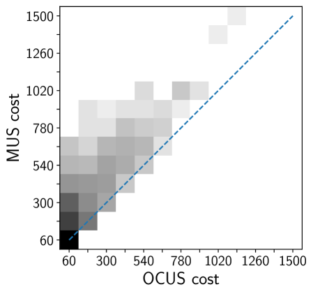
Figure 1: Q1 - Explanation quality comparison of optimal versus subset-minimal explanations in the generated puzzle explanation sequences.

8.2 Information Re-use

To answer Q2, we compare the effect of incrementality when generating a sequence of explanations. Next to (1) OCUS, we also include (2) the bounded OCUS (OCUS_Bound) algorithm, where we call the OCUS algorithm for every literal in every step, but we reuse information by giving it the current best bound $f(S_{best})$ and iterating over the literals that performed best in the previous call first; and (3) the split OCUS (OCUS_Split) approach, where we split up the computations by iteratively selecting the most promising literal and expanding only one hitting set for it, then re-evaluating the most promising literal and so forth.

8.2.1 Incremental versus Non-incremental Explanation Generation

Preliminary experiments have shown that incrementality by keeping track of the hitting sets using the MIP solver significantly outperforms bootstrapping satisfiable subsets. Therefore, in the experiments, we only show results on incrementality using MIP solvers.

For OCUS, incrementality (+Incr) is achieved by reusing the same MIP hitting set solver throughout the explanation calls, as explained in Section 7.1. Methods OCUS_Bound and OCUS_Split use a separate hitting set solver for every literal to explain. Each hitting set solver can similarly be made incremental (with respect to its own literal) across the explanation calls (+Incr.), or not.

Figure 2 depicts the number of instances fully explained through time before the given 1-hour timeout. In each configuration depicted, we use a single SAT-based Grow in the CorrSubsets procedure. The same color is used for the same OCUS algorithms, with a full line for the incremental version and a dashed line for the non-incremental one.

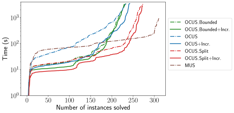
Figure 2: Time to generate a full explanation sequence with a single SAT grow call in the CorrSubsets procedure for incremental and non-incremental OCUS algorithms. Incrementality improves the number of instances solved and the time required to solve them for all O(C)US algorithms.

If we compare all configurations, we see that OCUS is faster than the plain MUS-based implementation for simpler instances. MUS is able to explain more instances than all OCUS versions, as it solves a simpler problem (with worse quality results as shown in Q1). OCUS_Bound is faster than OCUS for easier instances but explains about the same number of instances, and OCUS_Split is considerably faster and solves the most instances out of all OCUS algorithms.

The effect of introducing incrementality produces a speed-up in OCUS. For OCUS_Bound it is negligible and for OCUS_Split there is a speed-up in all but its most difficult instances. In general, we see that the curves of the incremental variants are located somewhat lower. The best runtimes are obtained with OCUS_Split+Incr., that is, using an incremental hitting set solver for every individual literal-to-explain separately and only expanding the literal that is most likely to provide a cost-minimal OCUS.

8.2.2 Instance-level Speed-up with Incrementality

Next, we analyze the speed-up of introducing incrementality per instance. Fig. 3 compares the time to generate a full sequence for the incremental variant with the non-incremental version for each puzzle of every OCUS configuration. Results in the upper triangle signify an improvement using incrementality, and the lower triangle indicates worse performance with incrementality.

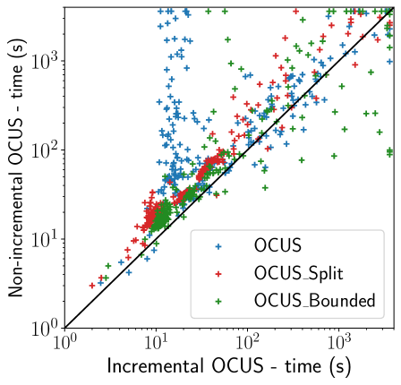
Figure 3: Q2 - Runtime comparison of introducing incrementality on the time to generate a whole explanation sequence with SAT-based Grow.

Taking a closer look at the results for OCUS, the story is similar to the results of Fig. 2. Many of the instances are explained quickly (around 10 to 20 seconds) by OCUS+Incr., whereas non-incremental OCUS takes much longer to explain some instances, even leading to a timeout.

Incrementality with OCUS_Split and OCUS_Bound produce marginal improvements on the runtime. Most of the instances lie close to the black line. Only a few instances are present in the lower triangle, for the incremental variant of OCUS_Bound. For these instances, OCUS_Bound+Incr. takes on average double the time to generate the first explanation step due to the overhead associated with introducing incrementality. The story is similar for the few instances where OCUS_Split+Incr. is slower than OCUS_Split.

8.3 Runtime Decomposition

To evaluate the time-critical components of OCUS (Q3), we decompose the time spent in each part of the OCUS algorithms in Table 6. We only included the runtimes of instances that do not time out for all methods to allow a fair comparison.

The table depicts for each configuration (1) the number of instances explained; (2) %OPT the percentage of time spent in the hitting set solver; (3) %SAT the percentage of time spent in the sat solver: (4) %CorrSS the percentage of time spent in the CorrSubsets procedure; and (5) $N_{sth}$the average total number of sets-to-hit computed. Each version of the OCUS algorithm uses the SAT-based grow in the CorrSubsets procedure (see Table 7).

Looking closer at the runtime decomposition, we observe that most of the time in all the OCUS algorithms is spent computing the optimal hitting sets. The results in the $N_{sth}$ column (top 3 rows versus incremental bottom 3 rows), highlight the decrease in the amount of sets-to-hit that need to be computed when adding incrementality, in our case, re-using the MIP solver between explanation steps. Indeed, similar to the results of Example 6, the OCUS algorithms do not need to recompute the previously derived sets-to-hit, and will therefore start with a good candidate hitting set at the beginning of an explanation step.

config explained %OPT %SAT %CorrSS $N_{sth}$ OCUS [233 / 403] 96.65% 3.01% 0.35% 6245 OCUS_Bound [229 / 403] 86.86% 12.31% 0.83% 9310 OCUS_Split [273 / 403] 88.58% 10.41% 1.01% 7480 OCUS+Incr. [242 / 403] 99.16% 0.78% 0.06% 405 OCUS_Bound+Incr. [233 / 403] 95.95% 3.94% 0.1% 1538 OCUS_Split+Incr. [272 / 403] 96.28% 3.42% 0.3% 1713 MUS [311 / 403] — — — —

Table 6: Runtime decomposition of core parts of O(C)US with the SAT-based grow. On the left, most of the computational time is spent in computing more optimal (constrained) hitting sets, while on the right, the runtime is shifted towards higher quality correction subsets. Incrementality, by re-using the same MIP solver throughout the explanation steps, helps to drastically reduce the average number of sets-to-hit $N_{sth}$.

8.4 Correction Subset Extraction

As Table 6 table shows, most time is spent computing the optimal hitting sets. Hence, there is potential in reducing its effort by computing better or more correction subsets, thereby having better collections of sets-to-hit. This induces a trade-off between the efficiency of the Grow strategy, the quality of the produced satisfiable subset as well as the corresponding sets-to-hit generated by the CorrSubsets procedure. In this section, we evaluate whether an efficient Grow-call is able to balance the efficiency and the quality of the produced satisfiable subset. Second, we analyze whether the enumeration of multiple, ideally $p$-disjoint, correction subsets reduces the time spent in the hitting set solver.

Thus, to answer Q4, we compare the incremental variants of OCUS, bounded OCUS, split OCUS, and only change the CorrSubsets strategy they use.

Efficient Correction Subset Enumeration

Extending the observation of Section 5.3.1 that a call to an efficient MaxSAT solver helps in finding maximally satisfiable subsets, we propose three additional variants of Algorithm 7:

1. The first variant, Multi-SAT, repeatedly grows with SAT and blocks the corresponding correction subset until no more correction subsets can be extracted.

2. The second variant is Multi-MaxSAT. This correction subset enumerator repeatedly grows using the domain-specific MaxSAT introduced in Section 5.3.1 until the updated subset $\mathcal{S}^{\prime}$ is no longer satisfiable.

3. The last variant Multi-SubsetMax-SAT repeatedly grows using the SubsetMax-SAT to balance the trade-off between efficiency and quality.

CorrSubsets Description SAT Extract a satisfiable model computed by the SAT solver. SubsetMax-SAT Extends the satisfiable subset computed by SAT by adding every remaining clause $c\in\mathcal{F}\setminus\mathcal{S}$ if $\mathcal{S}\cup\{c\}$ is satisfiable. Dom.-spec. MaxSAT Grow using an unweighted MaxSAT solver with domain-specific information, i.e. only previously derived facts and the original constraints (see Section 7.1). MaxSAT Full Grow with an unweighted MaxSAT solver using the full unsatisfiable formula $\mathcal{F}$. Multi SAT Repeatedly grow with SAT and block the corresponding correction subset until no more correction subsets can be extracted. Multi Dom.-spec. MaxSAT Repeatedly with Dom.-spec. MaxSAT and block the corresponding correction subset until no more correction subsets can be extracted. Multi SubsetMax-SAT Repeatedly grow with SubsetMax-SAT and block the corresponding correction subset until no more correction subsets can be extracted.

Table 7: Description of the correction subset procedures.

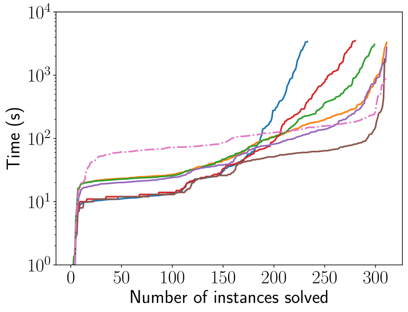
(a) OCUS_Bound+Incr.

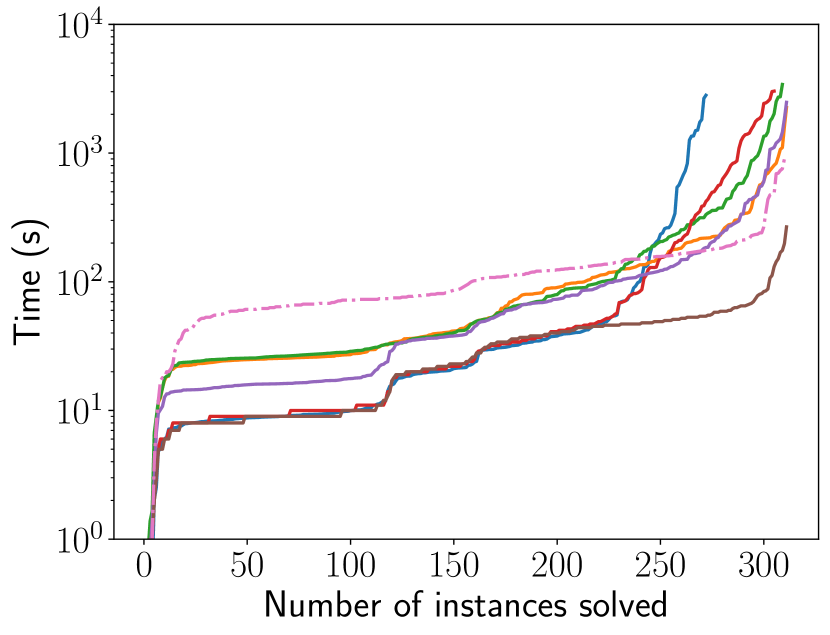
(b) OCUS_Split+Incr.

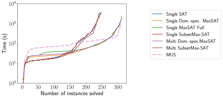
(c) OCUS+Incr. ———————————————————–

Figure 4: Average cumulative explanation time of correction subset configurations for the incremental O(C)US variants. The legends for each graph are ordered from the least instances explained (top) to the most instances explained (bottom).

Figure 4 depicts for each incremental OCUS algorithm, the number of instances solved across time for varying correction subset approaches. For OCUS+Incr., all MaxSAT-based methods for enumerating correction subsets provide similar results and are able to explain more instances than the rest. The story for OCUS_Split+Incr. and OCUS_Bound+Incr. is different. The best method for enumerating correction subsets with OCUS_Split+Incr. and OCUS_Bound+Incr. is Multi-SubsetMax-SAT. Multi-SubsetMax-SAT is able to consistently beat all other correction subset enumeration methods and is substantially faster than the naive MUS approach. To summarize, the best explanation sequence configuration corresponds to the iterated MIP-incremental approach of OCUS_Split+Incr. combined with Multi-SubsetMax-SAT.

Runtime Decomposition

We now look at the runtime decomposition in Table 8 for the best performing CorrSubsets configuration, i.e. Multi-SubsetMax-SAT, also for the non-incremental OCUS variants. For the non-incremental variants, we observe that the shift in computation from the hitting set solver to correction subset enumeration clearly reaps its benefits.

	Multi-SubsetMax-SAT
config	explained	%OPT	%SAT	%CorrSS	$\mathbf{N_{sth}}$
OCUS	[291 / 403]	68.15%	2.78%	29.07%	3649
OCUS_Bound	[311 / 403]	39.87%	6.53%	53.6%	29747
OCUS_Split	[311 / 403]	45.24%	3.62%	51.14%	28320
OCUS+Incr.	[245 / 403]	87.38%	1.03%	11.59%	402
OCUS_Bound+Incr.	[309 / 403]	81.57%	5.68%	12.76%	1251
OCUS_Split+Incr.	[311 / 403]	79.64%	1.77%	18.58%	1274
MUS	[311 / 403]	—	—	—	—

Table 8: Runtime decomposition of core parts of OCUS. On the left, most of the computation time is spent in computing more optimal (constrained) hitting sets, while on the right, the runtime is shifted toward higher-quality correction subsets.

Compared to Table 6, more instances are explained, and the computation is more balanced both for incremental and non-incremental OCUS algorithms. The non-incremental OCUS variants require considerably more correction subsets to be extracted and somewhat fewer in the incremental case. However, the number of instances explained is substantially higher for all OCUS configurations.

8.5 Efficiency of Single Step O(C)US, Instantaneous and Step-wise

In this section, we analyze whether the algorithms we developed could be fit for an interactive context. By an interactive context, we consider two types of settings. First, a user may want an immediate explanation step for the given CSP, and second, a user is asking for the next step, and the next, and so forth.

Table 9 depicts Multi-SubsetMax-SAT the best performing CorrSubsets procedure of Fig. 4. For each OCUS algorithm, we compute the average time to produce the first explanation step $\overline{t_{1}}$ (instantaneous), the average time to generate one step-wise explanation $\overline{t_{step}}$, and the explanation time quantiles 25 up to 100, where quantile 100 $q_{100}$ symbols the most expensive step to generate over all the problem instances.

Multi-SubsetMax-SAT config $\mathbf{\overline{t_{1}}}$ $\mathbf{\overline{t_{step}}}$ $\mathbf{q_{25}}$ $\mathbf{q_{50}}$ $\mathbf{q_{75}}$ $\mathbf{q_{95}}$ $\mathbf{q_{98}}$ $\mathbf{q_{100}}$ OCUS 3.41 2.54 0.51 0.77 1.39 8.37 18.50 523.67 OCUS_Bound 1.70 1.35 0.58 0.92 1.88 3.67 4.45 7.34 OCUS_Split 0.92 1.31 0.54 0.90 1.84 3.58 4.24 6.11 OCUS+Incr. 4.33 3.66 0.27 0.42 0.72 8.69 21.46 3452.20 OCUS_Bound+Incr. 3.22 0.58 0.39 0.51 0.67 1.07 1.57 17.58 OCUS_Split+Incr. 2.58 0.45 0.32 0.43 0.54 0.70 1.04 18.05

Table 9: Non-timed out instances: Decomposition of runtime for individual explanations into time to generate the first explanation step ($t_{1}$), the average time to produce an additional explanation step $\overline{t_{expl}}$ and $q_{xx}$ the quantiles of the explanation times.

For the non-incremental variants, in the upper part of Table 9, OCUS is able to compute part of the explanations faster than the other OCUS configurations. We see, however, that both incremental and non-incremental OCUS still take a lot of time for some explanations compared to the other OCUS-based algorithms.

In the case of OCUS_Bound, the time to the first explanation reflects how important the ordering of literals to explain is for quickly finding a good bound on the cost of the next best explanation.

Logic Grid Puzzles

In Table 10, we detail the runtime for explaining the logic grid puzzles of ? (?). In that work, due to the use of heuristics for finding low-cost explanations, the full explanation of a puzzle took between ‘15 minutes and a few hours’. Explaining the pasta puzzle takes less than 5 minutes using OCUS_Split+Incr. with Multi-SubsetMax-SAT as CorrSubsets procedure. Not only can we generate optimal explanations with respect to a given cost function, but we can also quickly provide an initial explanation and additional explanations. This suggests that our methods can be integrated into an interactive setting.

puzzle	$\mathbf{t_{1}}$	$\mathbf{\overline{t_{expl}}}$	$\mathbf{t_{tot}}$
origin	1.07s	0.29s	43.05s
p12	1.25s	0.43s	63.85s
p13	1.20s	0.37s	56.22s
p16	1.04s	0.27s	40.98s
p18	1.14s	0.16s	23.32s
p19	3.76s	0.55s	137.08s
p20	1.14s	0.16s	23.38s
p25	1.12s	0.26s	38.32s
p93	1.13s	0.32s	47.83s
pasta	0.60s	2.98s	286.03s

Table 10: Runtime decomposition of Logic Grid Puzzles of ? (?) into time to generate the first explanation step ($t_{1}$), the average time to produce an additional explanation step $\overline{t_{expl}}$, and time to generate a full explanation sequence $t_{tot}$.

config $\#$none $\#$timed out $\mathbf{\overline{\raisebox{0.0pt}[1.2pt]{{\text{\small\%}} expl}}}$ OCUS 3 112 44.57 OCUS_Bound 32 92 35.21 OCUS_Split 15 92 43.43 OCUS+Incr. 4 158 52.94 OCUS_Bound+Incr. 44 94 31.98 OCUS_Split+Incr. 15 92 49.45

Table 11: Timed out instances: $\#$none is the number of instances where no explanations step was found before the time out, $\#$timed out is the number of instances that timed out, $\overline{\raisebox{0.0pt}[9.0pt]{{\small\%} expl}}$ is the average percentage of literals explained.

The next step is to find out what causes instances to timeout before the full explanation sequence has been generated with Multi-SubsetMax-SAT for all OCUS configurations.

Timed out Instances

Most of the instances that timed out had on average more literals to explain than those that did not. Table 11 provides more context about the timed out instances:

• $\#$timed out is the number of instances that have timed out.

• $\#$none is to the number of instances where no explanation step was generated.

• $\mathbf{\overline{\raisebox{0.0pt}[1.2pt]{{\text{\small\%}} expl}}}$ is the average percentage of literals that were explained before the instance timed out.

In Fig. 5 we specifically report the average time taken to generate a first explaining step ($\mathbf{\overline{t_{1}}}$) for all configurations.

Note from Table 11 that OCUS(+Incr.) has the smallest number of instances where no explanation was found. Unlike OCUS_Bound(+Incr.) and OCUS_Split(+Incr.), OCUS(+Incr.) does not need to iterate over the many literals to explain in order to find a good bound on the cost of the next best explanation step. Furthermore, we observe that OCUS(+Incr.) is the fastest at generating a first explanation step with many outliers close to the .

Similar to the observations in Section 8.2.2, incrementality has a high impact on the time to explain an instance for all OCUS configurations. Adding incrementality to all OCUS configurations results in more instances with no explanation found than without incrementality. However, incrementality helps to explain more literals, except for OCUS_Bound, which first requires computing many OUSs before the best one is found. A similar trend can be seen in Fig. 5, where the introduction of incrementality increases the time to generate a first explanation step. Second, OCUS_Bound depends on a good ordering of the literals, which can change at any explanation step in the sequence.

Figure 5: Average time to a first explanation step $\mathbf{\overline{t_{1}}}$.

To conclude, for an interactive context where the user asks for an immediate explanation, OCUS_Split will be the fastest to compute an explanation step. If the user explores the sequence of explanations and repeatedly asks for additional explanations, OCUS_Split+Incr. will be able to capitalise on incrementality to bring the average time close to real time.

9 Conclusion and Future Work

In this paper, we tackled the problem of efficiently generating explanations that are optimal with respect to a cost function. For that, we introduced algorithms that replace the many calls to an unsatisfiable core extractor of ? (?), with a single call to an optimal constrained unsatisfiable subset (OCUS). Our algorithm for computing OCUSs uses the implicit hitting set duality between Minimum Correction Subsets and Minimal Unsatisfiable Subsets. We propose two additional variants for the ‘exactly one of’ constraint used in step-wise explanation generation. The main bottleneck of these approaches is having to repeatedly compute optimal hitting sets. To compensate, we have developed methods for enumerating correction subsets that explore the trade-off between efficiency and quality of the subsets generated. An open question in an interactive setting is whether there are other methods of enumerating correction subsets that are better suited to reducing the time to first explanation and the average explanation time.

To efficiently generate the whole explanation sequence, we introduced incrementality, which allows the reuse of computed information, i.e. satisfiable subsets remain valid from one explanation call to another. In the case of OCUS for explanation sequence generation, where the underlying hitting set solver is MIP-based, we instantiate the MIP solver once for all explanation steps and keep track of computed sets-to-hit. However, MIP solvers do not natively support non-linear cost functions. Therefore, the current implementation of OCUS may not be able to fully capture the complexity of what constitutes a good explanation due to the limitations of the cost functions we can encode. Furthermore, the question of which interpretability metric to use to characterise understandable explanations remains open.

The concept of (incremental) OCUS is not limited to explaining satisfaction problems. We are also interested in exploring other applications, such as configuration and machine learning, where it is necessary to compute not only minimal but also optimal unsatisfiable subsets. For example, a potential avenue for future work is how these explanation generation methods map to a constraint optimisation setting where branching or searching is required to solve the problem at hand. The synergies of our approach with the more general problem of QMaxSAT (?) is another open question.

Finally, for interactive settings such as interactive tutoring systems, we are able to generate explanations in near real time (less than a second) using OCUS_Split. Another question is how to distribute the computation across multiple cores to parallelize the computation to further speed up the generation of explanations.

Acknowledgments

This research received partial funding from the Flemish Government (AI Research Program); the FWO Flanders project G070521N; and funding from the European Research Council (ERC) under the European Union’s Horizon 2020 research and innovation program (Grant No. 101002802, CHAT-Opt).

A Puzzle Data

		Properties of instances
		n	avg. $\#$ clauses	avg. $\#$ lits-to-explain
puzzle type	instance
logic	pasta	1	4572	96
	150	8	7535	150
	250	1	17577	250
sudoku	9x9-easy	25	14904	497
	9x9-simple	25	14904	497
	9x9-intermediate	25	14904	501
	9x9-expert	25	14904	505
demystify	binairo	156	16759	99
	garam	10	14486	756
	kakurasu	1	226	16
	kakuro	6	6961	240
	killersudoku	13	3609685	729
	miracle	1	59331	729
	nonogram	1	9813	36
	skyscrapers	16	17991	159
	star-battle	5	7533	82
	sudoku	76	34143	729
	tents	4	18644	476
	thermometer	1	1227	36
	x-sums	1	109717	729

Table 12: Characteristics of puzzle instances

References

- Alrabbaa, Baader, Borgwardt, Koopmann, and Kovtunova Alrabbaa, C., Baader, F., Borgwardt, S., Koopmann, P., and Kovtunova, A. (2021). Finding good proofs for description logic entailments using recursive quality measures. Automated Deduction-CADE, 12–15.
- Baader, Horrocks, and Sattler Baader, F., Horrocks, I., and Sattler, U. (2004). Description logics. In Handbook on ontologies, pp. 3–28. Springer.
- Bacchus and Katsirelos Bacchus, F., and Katsirelos, G. (2015). Using minimal correction sets to more efficiently compute minimal unsatisfiable sets. In Computer Aided Verification: 27th International Conference, CAV 2015, San Francisco, CA, USA, July 18-24, 2015, Proceedings, Part II, pp. 70–86. Springer.
- Bacchus and Katsirelos Bacchus, F., and Katsirelos, G. (2016). Finding a collection of muses incrementally. In Integration of AI and OR Techniques in Constraint Programming: 13th International Conference, CPAIOR 2016, Banff, AB, Canada, May 29-June 1, 2016, Proceedings 13, pp. 35–44. Springer.
- Bendík and Černá Bendík, J., and Černá, I. (2020a). Must: minimal unsatisfiable subsets enumeration tool. In Tools and Algorithms for the Construction and Analysis of Systems: 26th International Conference, TACAS 2020, Held as Part of the European Joint Conferences on Theory and Practice of Software, ETAPS 2020, Dublin, Ireland, April 25–30, 2020, Proceedings, Part I 26, pp. 135–152. Springer.
- Bendík and Černá Bendík, J., and Černá, I. (2020b). Replication-guided enumeration of minimal unsatisfiable subsets. In Principles and Practice of Constraint Programming: 26th International Conference, CP 2020, Louvain-la-Neuve, Belgium, September 7–11, 2020, Proceedings 26, pp. 37–54. Springer.
- Biere, Heule, van Maaren, and Walsh Biere, A., Heule, M., van Maaren, H., and Walsh, T. (2009). Handbook of Satisfiability.
- Bogaerts, Gamba, Claes, and Guns Bogaerts, B., Gamba, E., Claes, J., and Guns, T. (2020). Step-wise explanations of constraint satisfaction problems. In Proceedigns of ECAI, pp. 640–647.
- Bogaerts, Gamba, and Guns Bogaerts, B., Gamba, E., and Guns, T. (2021). A framework for step-wise explaining how to solve constraint satisfaction problems. Artificial Intelligence, 300, 103550.
- Chakraborti, Sreedharan, Zhang, and Kambhampati Chakraborti, T., Sreedharan, S., Zhang, Y., and Kambhampati, S. (2017). Plan explanations as model reconciliation: moving beyond explanation as soliloquy. In Proceedings of IJCAI, pp. 156–163.
- Čyras, Letsios, Misener, and Toni Čyras, K., Letsios, D., Misener, R., and Toni, F. (2019). Argumentation for explainable scheduling. In Proceedings of AAAI, pp. 2752–2759.
- Davies and Bacchus Davies, J., and Bacchus, F. (2013). Exploiting the power of MIP solvers in MAXsat. In Proceedings of SAT, pp. 166–181.
- Dershowitz, Hanna, and Nadel Dershowitz, N., Hanna, Z., and Nadel, A. (2006). A scalable algorithm for minimal unsatisfiable core extraction. In Proceedings of SAT, pp. 36–41.
- Espasa, Gent, Hoffmann, Jefferson, and Lynch Espasa, J., Gent, I. P., Hoffmann, R., Jefferson, C., and Lynch, A. M. (2021). Using small muses to explain how to solve pen and paper puzzles. ArXiv, abs/2104.15040.
- Robustness and of Artificial Intelligence FET (2019). Fetproact-eic-05-2019, fet proactive: emerging paradigms and communities, call.. Horizon 2020 Framework Programme.
- Fox, Long, and Magazzeni Fox, M., Long, D., and Magazzeni, D. (2017). Explainable planning. In Proceedings of IJCAI’17-XAI.
- Freuder, Likitvivatanavong, and Wallace Freuder, E. C., Likitvivatanavong, C., and Wallace, R. J. (2001). Explanation and implication for configuration problems. In IJCAI 2001 workshop on configuration, pp. 31–37.
- Frisch, Harvey, Jefferson, Martinez-Hernandez, and Miguel Frisch, A. M., Harvey, W., Jefferson, C., Martinez-Hernandez, B., and Miguel, I. (2008). Essence: A constraint language for specifying combinatorial problems. Constraints, 13(3), 268–306.
- Gamba, Bogaerts, and Guns Gamba, E., Bogaerts, B., and Guns, T. (2021). Efficiently explaining CSPs with unsatisfiable subset optimization. In Zhou, Z.-H. (Ed.), Proceedings of the Thirtieth International Joint Conference on Artificial Intelligence, IJCAI-21, pp. 1381–1388. International Joint Conferences on Artificial Intelligence Organization. Main Track.
- Gershman, Koifman, and Strichman Gershman, R., Koifman, M., and Strichman, O. (2008). An approach for extracting a small unsatisfiable core. Formal Methods in System Design, 33(1-3), 1–27.
- Goldberg and Novikov Goldberg, E., and Novikov, Y. (2003). Verification of proofs of unsatisfiability for CNF formulas. In Proceedings of DATE, pp. 10886–10891.
- Guidotti, Monreale, Ruggieri, Turini, Giannotti, and Pedreschi Guidotti, R., Monreale, A., Ruggieri, S., Turini, F., Giannotti, F., and Pedreschi, D. (2018). A survey of methods for explaining black box models. ACM computing surveys (CSUR), 51(5), 1–42.
- Gunning Gunning, D. (2017). Explainable artificial intelligence (XAI). Defense Advanced Research Projects Agency, 2.
- Hamon, Junklewitz, and Sanchez Hamon, R., Junklewitz, H., and Sanchez, I. (2020). Robustness and explainability of artificial intelligence. Publications Office of the European Union.
- Hildebrandt, Castillo, Celis, Ruggieri, Taylor, and Zanfir-Fortuna Hildebrandt, M., Castillo, C., Celis, E., Ruggieri, S., Taylor, L., and Zanfir-Fortuna, G. (Eds.). (2020). Proceedings of FAT*.
- Huang Huang, J. (2005). Mup: A minimal unsatisfiability prover. In Proceedings of the Asia and South Pacific Design Automation Conference, ASP-DAC, pp. 432– 437 Vol. 1.
- Ignatiev, Janota, and Marques-Silva Ignatiev, A., Janota, M., and Marques-Silva, J. (2016). Quantified maximum satisfiability. Constraints, 21(2), 277–302.
- Ignatiev, Morgado, and Marques-Silva Ignatiev, A., Morgado, A., and Marques-Silva, J. (2018). PySAT: A Python toolkit for prototyping with SAT oracles. In SAT, pp. 428–437.
- Ignatiev, Narodytska, and Marques-Silva Ignatiev, A., Narodytska, N., and Marques-Silva, J. (2019). Abduction-based explanations for machine learning models. In Proceedings of AAAI, pp. 1511–1519.
- Ignatiev, Previti, Liffiton, and Marques-Silva Ignatiev, A., Previti, A., Liffiton, M., and Marques-Silva, J. (2015). Smallest MUS extraction with minimal hitting set dualization. In Proceedings of CP.
- Junker Junker, U. (2001). QuickXPlain: Conflict detection for arbitrary constraint propagation algorithms. In IJCAI’01 Workshop on Modelling and Solving problems with constraints.
- Kleine Büning and Bubeck Kleine Büning, H., and Bubeck, U. (2009). Theory of quantified boolean formulas. In Handbook of Satisfiability, pp. 735–760.
- Koopmann Koopmann, P. (2021). Two ways of explaining negative entailments in description logics using abduction. Explainable Logic-Based Knowledge Representation (XLoKR 2021).
- Langley, Meadows, Sridharan, and Choi Langley, P., Meadows, B., Sridharan, M., and Choi, D. (2017). Explainable agency for intelligent autonomous systems. In Twenty-Ninth IAAI Conference.
- Li and Manyà Li, C. M., and Manyà, F. (2021). MaxSAT, hard and soft constraints. In Handbook of satisfiability, pp. 903–927. IOS Press.
- Liao and Van Der Torre Liao, B., and Van Der Torre, L. (2020). Explanation semantics for abstract argumentation. In Computational Models of Argument, pp. 271–282. IOS Press.
- Liffiton, Previti, Malik, and Marques-Silva Liffiton, M. H., Previti, A., Malik, A., and Marques-Silva, J. (2016). Fast, flexible mus enumeration. Constraints, 21(2), 223–250.
- Liffiton and Sakallah Liffiton, M. H., and Sakallah, K. A. (2008). Algorithms for computing minimal unsatisfiable subsets of constraints. J. Autom. Reasoning, 40(1), 1–33.
- Lundberg and Lee Lundberg, S. M., and Lee, S.-I. (2017). A unified approach to interpreting model predictions. In Proceedings of NIPS, pp. 4765–4774.
- Lynce and Silva Lynce, I., and Silva, J. P. M. (2004). On computing minimum unsatisfiable cores. In Proceedings of SAT.
- Marques-Silva Marques-Silva, J. (2010). Minimal unsatisfiability: Models, algorithms and applications. In 2010 40th IEEE International Symposium on Multiple-Valued Logic.
- Marques-Silva, Heras, Janota, Previti, and Belov Marques-Silva, J., Heras, F., Janota, M., Previti, A., and Belov, A. (2013). On computing minimal correction subsets. In Twenty-Third International Joint Conference on Artificial Intelligence.
- Miller Miller, T. (2019). Explanation in artificial intelligence: Insights from the social sciences. Artificial Intelligence, 267, 1–38.
- Miller, Weber, and Magazzeni Miller, T., Weber, R., and Magazzeni, D. (Eds.). (2019). Proceedings of the IJCAI 2019 Workshop on Explainable Artificial Intelligence.
- Modgil, Toni, Bex, Bratko, Chesnevar, Dvořák, Falappa, Fan, Gaggl, García, et al. Modgil, S., Toni, F., Bex, F., Bratko, I., Chesnevar, C. I., Dvořák, W., Falappa, M. A., Fan, X., Gaggl, S. A., García, A. J., et al. (2013). The added value of argumentation. In Agreement technologies, pp. 357–403. Springer.
- Nightingale, Akgün, Gent, Jefferson, Miguel, and Spracklen Nightingale, P., Akgün, Ö., Gent, I. P., Jefferson, C., Miguel, I., and Spracklen, P. (2017). Automatically improving constraint models in savile row. Artificial Intelligence, 251, 35–61.
- Obeid, Obeid, Moubaiddin, and Obeid Obeid, M., Obeid, Z., Moubaiddin, A., and Obeid, N. (2019). Using description logic and abox abduction to capture medical diagnosis. In International Conference on Industrial, Engineering and Other Applications of Applied Intelligent Systems, pp. 376–388. Springer.
- Oh, Mneimneh, Andraus, Sakallah, and Markov Oh, Y., Mneimneh, M. N., Andraus, Z. S., Sakallah, K. A., and Markov, I. L. (2004). AMUSE: a minimally-unsatisfiable subformula extractor. In Proceedings of DAC, pp. 518–523.
- Reiter Reiter, R. (1987). A theory of diagnosis from first principles. AIJ, 32(1), 57–95.
- Rossi, van Beek, and Walsh Rossi, F., van Beek, P., and Walsh, T. (Eds.). (2006). Handbook of Constraint Programming, Vol. 2 of Foundations of Artificial Intelligence. Elsevier.
- Saikko, Wallner, and Järvisalo Saikko, P., Wallner, J. P., and Järvisalo, M. (2016). Implicit hitting set algorithms for reasoning beyond NP. In Proceedings of KR, pp. 104–113.
- Šešelja and Straßer Šešelja, D., and Straßer, C. (2013). Abstract argumentation and explanation applied to scientific debates. Synthese, 190(12), 2195–2217.
- Sqalli and Freuder Sqalli, M. H., and Freuder, E. C. (1996). Inference-based constraint satisfaction supports explanation. In AAAI/IAAI, Vol. 1, pp. 318–325.
- Ulbricht and Wallner Ulbricht, M., and Wallner, J. P. (2021). Strong explanations in abstract argumentation. In Proceedings of the AAAI Conference on Artificial Intelligence, Vol. 35, pp. 6496–6504.
- Vassiliades, Bassiliades, and Patkos Vassiliades, A., Bassiliades, N., and Patkos, T. (2021). Argumentation and explainable artificial intelligence: a survey. The Knowledge Engineering Review, 36.