ByteCover3: Accurate Cover Song Identification on Short Queries

Abstract

Deep learning based methods have become a paradigm for cover song identification (CSI) in recent years, where the ByteCover systems have achieved state-of-the-art results on all the mainstream datasets of CSI. However, with the burgeon of short videos, many real-world applications require matching short music excerpts to full-length music tracks in the database, which is still under-explored and waiting for an industrial-level solution. In this paper, we upgrade the previous ByteCover systems to ByteCover3 that utilizes local features to further improve the identification performance of short music queries. ByteCover3 is designed with a local alignment loss (LAL) module and a two-stage feature retrieval pipeline, allowing the system to perform CSI in a more precise and efficient way. We evaluated ByteCover3 on multiple datasets with different benchmark settings, where ByteCover3 beat all the compared methods including its previous versions.

Index Terms—  Cover song identification, ByteCover, local alignment loss, MaxMean similarity, short queries.

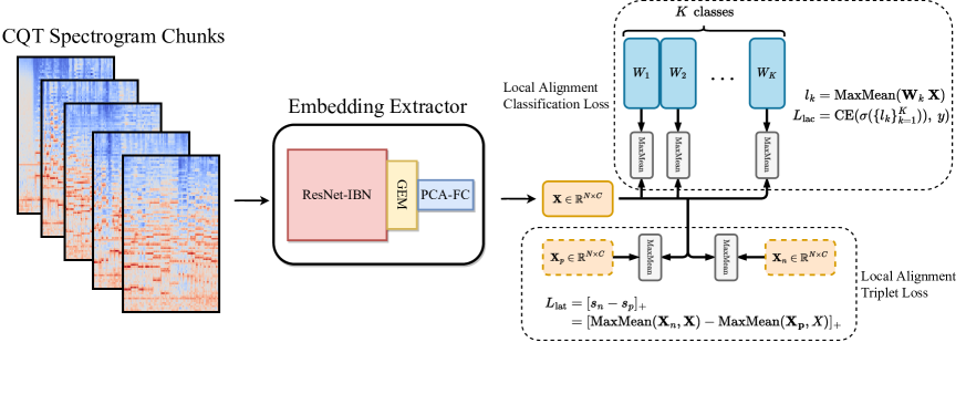
Fig. 1: The architecture of ByteCover3. ByteCover3 uses an embedding extractor to extract local features from the CQT chunks and optimizes the model using the LAL loss. The LAL loss consists of a LAL classification loss and a LAL triplet loss.

1 Introduction

Recent years have witnessed a successful use of deep learning methods in the task of cover song identification (CSI), i.e., finding cover versions of a given music track in a music database. These methods generally formulate CSI as either a classification problem [1, 2, 3] or a metric learning problem [4], or a combination of both [5, 6, 7], and then train deep neural networks to learn low-dimensional features from different representations of audio. The features are then indexed and retrieved, where the distances between features are used to measure the similarities of songs. Deep learning models have proved their capability in learning discriminative and robust features, boosting the accuracy of CSI by a large margin compared to traditional methods based on handcrafted features.

Despite of the promising progress above, one challenge remains for CSI in real-world applications, which is that most existing methods only consider situations when the query and the database item are both full-length music tracks with a typical duration of several minutes. Nevertheless, in many real-world scenarios, the task is to identify short music queries which are, for example, tens of seconds long, against full-length database songs. For instance, massive short videos with less-than-one-minute length have been created and uploaded to short video platforms such as TikTok in the past years, where a large proportion of these videos are accompanied by a carefully-selected music track that may be a remixed or cover fragment of an original music. For copyright management and reporting purpose, platforms need to identify these cover fragments. Unfortunately, as shown in section 3, most existing CSI systems failed in the experiments of identifying short queries. An explanation for such incapability is that current CSI methods are mostly equipped with a global pooling layer to aggregate the information from all time sections, and then generate a global embedding for each song as the CSI feature. However, when matching a short music clip to a full-length recording, there will be some irrelevant sections in the full-length recording that may create noises in the embedding, which pose a negative impact on the similarity measurement between features.

To solve this problem, an intuitive idea is to extract local features from both queries and database items, and calculate the similarity between two songs based only on the local features that have high matching score, thus avoiding the interference from irrelevant sections. This idea has been considered in a few traditional CSI works [8, 9, 10, 11, 12]. However, due to the limited discriminative capacity and robustness of handcrafted features, as well as the high complexity in performing efficient indexing and retrieval, traditional CSI methods are generally only applicable for small databases (e.g., the database used in [10] contains only 2,484 recordings) or simplified scenarios (e.g., [11] can only identify live versions of songs from known artists), while their performances for the general CSI task against large databases are poor (or have not been reported). In [13], Zalkow et al. made the first attempt to employ deep learning for short-query CSI and used convolutional neural networks (CNNs) to compress the input features. However, the databases used in [13] are still limited to thousands of audio recordings or even less, and its usability in real-world applications is unverified.

In this paper, we extend our previous works of ByteCover [5] and ByteCover2 [6], and present the new version of our CSI system, ByteCover3, to solve the problem of identifying short music queries against a industry-scale database of full-length recordings. Different from existing works that rely on global features [4, 2, 14, 5, 6], ByteCover3 is designed to learn a set of deep local embeddings (or features) from each audio and uses the matching of local embeddings to accomplish the identification of short queries against full songs. To optimize the matching of local features, we propose a new loss termed local alignment loss (LAL) and apply it in our multi-loss paradigm first introduced in ByteCover [5]. LAL constitutes one of the major contributions of ByteCover3, and by using the LAL loss, the performance of CSI can be significantly improved. Moreover, to improve the efficiency of feature matching, a two-stage feature retrieval pipeline, which consists of an approximate nearest neighbor (ANN) stage and a re-ranking stage, is also designed. This consists of our second contribution.

2 ByteCover3

The overall architecture of ByteCover3 is illustrated in Fig. 1. ByteCover3 is inherited from ByteCover and ByteCover2 and adopts a multi-loss learning paradigm for CSI. One of the major settings that differs it from previous works lies in the use of local features. In this section, we first describe the extraction of local features and then introduce our main contributions, i.e., the LAL loss for local feature matching and the two-stage feature retrieval pipeline.

2.1 Local Feature Extraction

To extract local features from each recording, we first resample the audio to $22,050$ Hz and split it into $N$ short chunks with a length of $20$ seconds and a overlap of $10$ seconds. For each chunk, we calculate a constant-Q transform (CQT) spectrogram with the number of bins per octave and the hop size set to $12$ and $512$ respectively, using Hann window as the window function. The CQT spectrograms are then downsampled with an averaging factor of $100$ along the time axis to reduce the computation cost. Therefore, the input audio is processed into a compressed $N$-chunk CQTs $\mathbf{S}\in\mathbb{R}^{N\times F\times T}$, where $N$ is the number of chunks, $F$ is the number of CQT bins ($84$ in our setting), and $T$ is the number of frames in each chunk.

The ResNet-IBN model [5], which replaces the residual connection blocks of ResNet50 [15] with the instance-batch normalization (IBN) blocks, is then applied as the backbone to extract local embeddings from the input CQTs. In ByteCover3, our ResNet-IBN follows the original ByteCover setting, except that a 3-D input $\mathbf{S}\in\mathbb{R}^{N\times F\times T}$ is taken instead of the original 2-D input. The output of ResNet-IBN before the global generalized mean (GeM) pooling layer is hence a 4-D embedding ${\mathbf{Z}}\in\mathbb{R}^{N\times C\times H\times W}$, where $C$ is the number of output channels, $H$ and $W$ are the spatial sizes along the frequency and time axes respectively. In practice, we set $C=2048$, $H=6$ and $W=\nicefrac{{T}}{{8}}$. Finally, the temporal and frequency axes of $\mathbf{Z}$ are integrated by the GeM pooling operation and a dimensionality reduction module, i.e., PCA-FC [6], is utilized on the channel dimension to obtain the compacted final embedding ${\mathbf{X}}\in\mathbb{R}^{N\times 512}$, which contains $N$ local features from the original audio, as opposed to ByteCover and ByteCover2 that only adopted a single global embedding.

2.2 The Local Alignment Loss

Existing CSI methods generally employ either a classification loss (e.g., softmax loss) or a metric learning loss (e.g., triplet loss) or a combination of them as the optimization objective during training. Nevertheless, as these methods only rely on a single global vector for each music track, their loss functions are limited to measuring similarities between two vectors (e.g. dot product or cosine similarity). Whereas in our case, we wish to compare two sequences of vectors that contain different number of local features, which requires a new similarity measure. To address this problem, we propose a novel loss design called Local Alignment Loss (LAL) $\mathcal{L}_{\operatorname{lal}}$ consisting of a classification loss $\mathcal{L}_{\operatorname{lac}}$ and a triplet loss $\mathcal{L}_{\operatorname{lat}}$.

We first introduce a similarity measure termed MaxMean inspired by [12]: let $\mathbf{X}\in\mathbb{R}^{M\times C}$ and $\mathbf{Y}\in\mathbb{R}^{N\times C}$ denote two $C$-dimensional feature sequences that each contain $M$ and $N$ local features ($M$ and $N$ could be highly different). For each local feature $\{\mathbf{x}_{i}\}_{i=1}^{M}\in\mathbb{R}^{1\times C}$ in $\mathbf{X}$, we calculate the cosine similarity between $\mathbf{x}_{i}$ and all the local features $\{\mathbf{y}_{i}\}_{j=1}^{N}\in\mathbb{R}^{1\times C}$ in $\mathbf{Y}$, and regard the maximal value as the similarity measure $s_{i}$ for $\mathbf{x}_{i}$:

$$s_{i}=\max(\cos(\mathbf{x}_{i},\mathbf{y}_{j})),\leavevmode\nobreak\ j=1,\dots,N,$$ (1)

and the final similarity score is obtained by taking average over all the similarity measures, i.e., $\operatorname{MaxMean}(\mathbf{X},\mathbf{Y})=\frac{1}{M}\sum_{i=1}^{M}s_{i}$. The shorter local feature is always regraded as the first operand, because the MaxMean operator is non-commutative. Since only the maximal value of all the matching scores from $\mathbf{x}_{i}$ to $\mathbf{Y}$ is considered, we can avoid the distractions of local features in $\mathbf{Y}$ that are irrelevant to $\mathbf{x}_{i}$.

With the MaxMean measure described above, we then illustrate how the original classification loss in previous ByteCover [5] is transformed to the novel LAL. Recall in ByteCover, the classification loss $\mathcal{L}_{cls}$ is defined as:

$$\mathcal{L}_{cls}=\operatorname{CE}(\sigma(\mathbf{W}\mathbf{f}^{\mathrm{T}}),\leavevmode\nobreak\ y)=\operatorname{CE}(\sigma(\{\mathbf{w}_{k}\mathbf{f}^{\mathrm{T}}\}_{k=1}^{K}),\leavevmode\nobreak\ y),$$ (2)

where $\operatorname{CE}(\cdot,\cdot)$ is the cross entropy and $\sigma(\cdot)$ is the softmax function. We denote $y$ as the ground-truth label, $\mathbf{f}\in\mathbb{R}^{1\times C}$ as the global feature extracted from ResNet-IBN, and $\mathbf{W}\in\mathbb{R}^{K\times C}$ as the weight matrix in the linear layer before softmax that contains $K$ weight vectors $\{{\bf w}_{k}\}_{k=1}^{K}$ for classification.

To adapt $\mathcal{L}_{cls}$ to the novel MaxMean measure with the local features, we draw inspiration from [16] and consider $\mathbf{w}_{k}$ as a proxy feature representation of the $k^{\mathrm{th}}$ class. In this sense, the result of $\mathbf{w}_{k}\mathbf{f}^{\mathrm{T}}$ can be interpreted as the similarity score between two features $\mathbf{w}_{k}$ and $\mathbf{f}$ based on dot product, which we argue can be replaced by the MaxMean metric. Specifically, our new local alignment classification loss $\mathcal{L}_{lac}$ is written as:

$$\mathcal{L}_{lac} =\operatorname{CE}(\sigma(\{\operatorname{logit}_{k}\}_{k=1}^{K}),y),$$ (3)

$$\operatorname{logit}_{k} =\operatorname{MaxMean}(\mathbf{X},\mathbf{W}_{k}),$$ (4)

where ${\bf X}\in\mathbb{R}^{N\times C}$ is the final embedding with $N$ local features extracted by ResNet-IBN, $\mathbf{W}\in\mathbb{R}^{K\times L\times C}$ is a trainable weight matrix in the linear layer before softmax and ${\bf W}_{k}\in\mathbb{R}^{L\times C}$ denotes the proxy representation for class $k$.

In addition to the classification loss, a triplet loss was also used in ByteCover, which is simply modified in ByteCover3 by replacing the Euclidean distance with MaxMean metric:

$$\mathcal{L}_{lat}=[\operatorname{MaxMean}({\bf X}_{n},{\bf X})-\operatorname{MaxMean}({\bf X}_{p},{\bf X})]_{+}.$$ (5)

Finally, our overall loss $\mathcal{L}_{lal}$ is given by $\mathcal{L}_{lal}=\mathcal{L}_{lac}+\mathcal{L}_{lat}$.

2.3 Two-Stage Feature Retrieval

An efficient feature retrieval pipeline is also critical for constructing a practical industrial-strength CSI system. Previous methods usually use an all-pairs strategy that includes computing the similarity between the query sample and each item in the database, which is time consuming. Moreover, there is a significant leap in complexity from the vector similarity measure ($\mathcal{O}(1)$) to the local alignment measure MaxMean ($\mathcal{O}(n^{2})$) [12], which makes the all-pairs strategy even worse for ByteCover3. To solve this problem, we propose a two-stage pipeline with a hierarchical searching strategy for the retrieval of deep local embeddings.

Given a query sample with $M$ local features, the first stage is to eliminate the database recordings that are highly unlikely to be a match. Specifically, for each local feature in the query, we search for its Top-$K$ nearest neighbors in the gallery of local features extracted in advance from all the database recordings, using the hierarchical navigable small world (HNSW) graphs [17], with $K$ set to $50$. This results in a candidate set of $M\times K$ local matches for the given query, based on which our second stage of feature retrieval is further performed. Suppose that the $M\times K$ local matches originate from $D$ database recordings ($D\leq M\times K$ since some local matches may original from the same recordings), and thus our second stage is to compare the given query with each of the $D$ candidate recordings, based on the MaxMean measure introduced above. The candidate recordings with the highest MaxMean similarities are finally outputted as the retrieval results.

In practical use, the query is typically less than 60s, and thus we have $M\leq 5$ as our local features are extracted every 20s with overlap of 10 seconds. Therefore, in the second stage we only need to calculate the MaxMean similarity for $M\times K\leq 250$ times, which is significantly less then the calculation needed in the all-pairs strategy.

3 Experiments

3.1 Evaluation Settings and Training Details

The evaluation of ByteCover3 was conducted based on three public datasets: (1) SHS100K [3], which is collected from the Second Hand Songs dataset, and consists of 8,858 cover groups and 108,523 recordings; (2) Covers80 [18], which contains 160 recordings of 80 songs, with 2 covers per song; and (3) Da-TACOS [4], which consists of 1000 cliques and 15,000 music performances.

More specifically, the training subset of SHS100K was used to train ByteCover3, and to obtain short music clips for training, we randomly cut a segment from each training recording, where the segment duration is uniformly sampled between $6$s and $60$s. These short music clips were then mixed with the original full-track training samples to form the final training set. The testing of ByteCover3 was performed in a query-retrieval mode using the testing subset of SHS100K, Cover80 and Da-TACOS. For each query, we constructed a query set consisting of the original full-track recording, and $9$ music clips randomly cut from it, with the duration being $6$, $10$, $15$, $20$, $25$, $30$, $40$, $50$ and $60$ seconds respectively.

For the training of ByteCover3, the weights of the trained ByteCover2 model were used to initialize the ResNet-IBN module. Similar to ByteCover2, we implemented ByteCover3 in Pytorch framework and trained it using the Adam Optimizer. The learning rate and the batch size were set to $0.001$ and $128$ respectively. Every training batch contained synthetic short samples and full-length samples mixed in a $1:1$ ratio to improve the stability of training process.

During testing, the mean average precision (mAP) and the mean rank of the first correctly identified cover (MR1) were used as evaluation metrics. In our calculation of mAP and MR1, we set the similarity values to 0 for the database items that are blocked in the first retrieval stage.

Moreover, since the queries were derived from snippets of some recordings in the result list, we ignored these recordings when calculating the evaluation metrics, to ensure that there is no leakage in the final detection performance.

Fig. 2: Length of Queries vs. Performance.

3.2 Comparison on Performance and Efficiency

Fig. 2 displays the mAP results of ByteCover3 for different query lengths on the synthetic SHS100K test set, using Re-MOVE [19] and ByteCover2 [6] as compared methods. As illustrated in the figure, our ByteCover3 model achieves the best mAPs for all the query lengths. This clearly indicates the effectiveness of ByteCover3 for identifying short music queries. As for the task of identifying full-length recordings, our ByteCover3 is also competitive. As presented in Table 1 (the first three parts), the performances of ByteCover3 are comparable with the state-of-the-art method ByteCover2 [6] on all the three test sets in the full-length settings, even with an embedding size of $512$, which is smaller than those of ByteCover and ByteCover2.

To measure the effect of our proposed LAL loss on the performance of CSI, we conducted an ablation study on SHS100K-TEST for query length of 30s, by comparing ByteCover3 with ByteCover2 and ByteCover2 + Local. ByteCover2 + Local modifies ByteCover2 with local features as done in ByteCover3, and it differs from ByteCover3 in that it does not use the LAL loss. The lower part of Table 1 gives the comparison results. As shown in the table, ByteCover3 achieves the highest mAP and lowest MR1 among the methods, which obviously proves the importance of LAL for short-query CSI.

Our last experiment is to test the time consumption of CSI, using the same setting as in [6]. As shown in Table 2, even equipped with local features, the retrieval speed of ByteCover3 is still at the same scale with ByteCover2 using an embedding size of $128$. We owe this to the use of our two-stage feature retrieval pipeline. Please note that the inference time of ByteCover3 is two times longer than ByteCover2, because we split the input CQT spectrogram into chunks and the complexity of feature extraction is higher. However, the total time consumption of ByteCover3 is sitll similar with that of ByteCover2-128.

Model	#Dims. $\downarrow$	mAP $\uparrow$	MR1 $\downarrow$
	Covers80  [18] (full)
CQT-Net [2]	300	0.840	3.85
ByteCover [5]	2048	0.906	3.54
ByteCover2  [6]	1536	0.928	3.23
ByteCover3	512	0.927	3.32
	Da-TACOS [4] (full)
ReMOVE [19]	2048	0.525	-
ByteCover2  [6]	1536	0.791	19.2
ByteCover3	512	0.703	36.7
	SHS100K-TEST  [3] (full)
CQT-Net [2]	300	0.655	54.9
ByteCover [5]	2048	0.836	47.3
ByteCover2  [6]	1536	0.864	39.0
ByteCover3	512	0.8242	37.0
	SHS100K-TEST  [3] (30 Secs)
ByteCover2 [6]	1536	0.430	244.1
ByteCover2 + local	1536	0.413	212.8
ByteCover3	512	0.734	99.9

Table 1: Performance on different datasets and ablation study on 30 seconds version SHS100K-TEST.

	Embedding Extraction		Retrieval	Total
	Preprocess	Inference
Re-MOVE [19]	5352 $\pm$ 123	60 $\pm$ 8.7	360 $\pm$ 73	5772
ByteCover2-1536 [6]	285 $\pm$ 31	108 $\pm$ 15.2	2601 $\pm$ 384	2994
ByteCover2-128 [6]	292 $\pm$ 39	105 $\pm$ 13.5	141 $\pm$ 13	538
ByteCover3-512	290 $\pm$ 30	209 $\pm$ 14.6	237 $\pm$ 19	731

Table 2: Time consumption of different models in data preprocessing, model inference and retrieval phases respectively.

4 Conclusion

In this paper, we propose to combine local feature matching and two-stage feature retrieval for efficient CSI of short music queries. A new loss termed LAL is designed to optimize the similarity measurement between songs with different length. Experimental results show that ByteCover3 outperforms all benchmark models on three synthetic datasets for short-query CSI, while being highly efficient in local embedding extraction and hierarchical retrieval. For future work, we are currently studying to apply ByteCover3 to other real-world applications such as set list identification, music matching with accurate timestamp and humming recognition.

References

- [1] Zhesong Yu, Xiaoshuo Xu, Xiaoou Chen, and Deshun Yang, “Temporal pyramid pooling convolutional neural network for cover song identification,” in Proceedings of the 28th International Joint Conference on Artificial Intelligence, 2019, pp. 4846–4852.
- [2] Z. Yu, X. Xu, X. Chen, and D. Yang, “Learning a representation for cover song identification using convolutional neural network,” in IEEE International Conference on Acoustics, Speech and Signal Processing (ICASSP), 2020, pp. 541–545.
- [3] Xiaoshuo Xu, Xiaoou Chen, and Deshun Yang, “Key-invariant convolutional neural network toward efficient cover song identification,” in IEEE International Conference on Multimedia and Expo, 2018, pp. 1–6.
- [4] F. Yesiler, J. Serrà, and E. Gómez, “Accurate and scalable version identification using musically-motivated embeddings,” in Proc. of the IEEE Int. Conf. on Acoustics, Speech and Signal Processing (ICASSP), 2020, pp. 21–25.
- [5] Xingjian Du, Zhesong Yu, Bilei Zhu, Xiaoou Chen, and Zejun Ma, “Bytecover: Cover song identification via multi-loss training,” in IEEE International Conference on Acoustics, Speech and Signal Processing (ICASSP). IEEE, 2021, pp. 551–555.
- [6] Xingjian Du, Ke Chen, Zijie Wang, Bilei Zhu, and Zejun Ma, “Bytecover2: Towards dimensionality reduction of latent embedding for efficient cover song identification,” in ICASSP 2022-2022 IEEE International Conference on Acoustics, Speech and Signal Processing (ICASSP). IEEE, 2022, pp. 616–620.
- [7] Shichao Hu, Bin Zhang, Jinhong Lu, Yiliang Jiang, Wucheng Wang, Lingcheng Kong, Weifeng Zhao, and Tao Jiang, “Wideresnet with joint representation learning and data augmentation for cover song identification,” 2022.
- [8] Meinard Müller, Frank Kurth, and Michael Clausen, “Audio matching via chroma-based statistical features.,” in International Society for Music Information Retrieval Conference, 2005.
- [9] Michael Casey, Christophe Rhodes, and Malcolm Slaney, “Analysis of minimum distances in high-dimensional musical spaces,” IEEE Transactions on Audio, Speech, and Language Processing, vol. 16, no. 5, pp. 1015–1028, 2008.
- [10] Peter Grosche and Meinard Müller, “Toward characteristic audio shingles for efficient cross-version music retrieval,” in 2012 IEEE International Conference on Acoustics, Speech and Signal Processing (ICASSP). IEEE, 2012, pp. 473–476.
- [11] Zafar Rafii, Bob Coover, and Jinyu Han, “An audio fingerprinting system for live version identification using image processing techniques,” in 2014 IEEE International Conference on Acoustics, Speech and Signal Processing (ICASSP). IEEE, 2014, pp. 644–648.
- [12] Kang Cai, Deshun Yang, and Xiaoou Chen, “Two-layer large-scale cover song identification system based on music structure segmentation,” in 2016 IEEE 18th International Workshop on Multimedia Signal Processing (MMSP). IEEE, 2016, pp. 1–6.
- [13] Frank Zalkow, Julian Brandner, and Meinard Müller, “Efficient retrieval of music recordings using graph-based index structures,” Signals, vol. 2, no. 2, pp. 336–352, 2021.
- [14] Guillaume Doras and Geoffroy Peeters, “Cover detection using dominant melody embeddings,” in Proceedings of the 20th International Society for Music Information Retrieval Conference, ISMIR 2019, 2019, pp. 107–114.
- [15] Kaiming He, Xiangyu Zhang, Shaoqing Ren, and Jian Sun, “Deep residual learning for image recognition,” in IEEE Conference on Computer Vision and Pattern Recognition, CVPR. 2016, pp. 770–778, IEEE Computer Society.
- [16] Yifan Sun, Changmao Cheng, Yuhan Zhang, Chi Zhang, Liang Zheng, Zhongdao Wang, and Yichen Wei, “Circle loss: A unified perspective of pair similarity optimization,” in Proceedings of the IEEE/CVF Conference on Computer Vision and Pattern Recognition, 2020, pp. 6398–6407.
- [17] Yu A Malkov and Dmitry A Yashunin, “Efficient and robust approximate nearest neighbor search using hierarchical navigable small world graphs,” IEEE transactions on pattern analysis and machine intelligence, vol. 42, no. 4, pp. 824–836, 2018.
- [18] D. P. W. Ellis and G. E. Poliner, “Identifying ‘cover songs’ with chroma features and dynamic programming beat tracking,” in Proc. of the IEEE Int. Conf. on Acoustics, Speech and Signal Processing (ICASSP), 2007, vol. IV, pp. 1429–1432.
- [19] Furkan Yesiler, Joan Serrà, and Emilia Gómez, “Less is more: Faster and better music version identification with embedding distillation,” in Proc. of the Int. Soc. for Music Information Retrieval Conf. (ISMIR), 2020.