Phase-Matching Quantum Key Distribution Without Intensity Modulation

Abstract

Quantum key distribution provides a promising solution for sharing secure keys between two distant parties with unconditional security. Nevertheless, quantum key distribution is still severely threatened by the imperfections of devices. In particular, the classical pulse correlation threatens security when sending decoy states. To address this problem and simplify experimental requirements, we propose a phase-matching quantum key distribution protocol without intensity modulation. Instead of using decoy states, we propose a alternative method to estimate the theoretical upper bound on the phase error rate contributed by even-photon-number components. Simulation results show that the transmission distance of our protocol could reach 305 km in telecommunication fiber. Furthermore, we perform a proof-of-principle experiment to demonstrate the feasibility of our protocol, and the key rate reaches 22.5 bit/s under a 45-dB channel loss. Addressing the security loophole of pulse intensity correlation and replacing continuous random phase with six- or eight-slice random phase, our protocol provides a promising solution for constructing quantum networks.

I Introduction

The fundamental principles of quantum mechanics open up endless and promising possibilities in fields such as communications, computing, and artificial intelligence [1, 2, 3, 4, 5, 6, 7, 8, 9]. Quantum key distribution (QKD) is a tool for distributing secret keys between two remote parties, and it makes information-theoretic secure communication possible, even if the potential eavesdropper has unlimited computational power [1, 2]. Over the past decades, various protocols have been proposed for paving the way toward quantum networks [10, 11, 12, 13, 14, 15, 16, 17, 18, 19]. Unfortunately, there are many security loopholes in QKD caused by the imperfections of experimental devices [20, 21, 22, 23, 24, 25, 26]. Measurement-device-independent (MDI) QKD removes all the side channels of the measurement unit [27]. Thus far, many theoretical and experimental breakthroughs have been made in MDI QKD [27, 28, 29, 30, 31, 32, 33, 34]. Twin-field QKD [35], a variant of MDI QKD, which uses single-photon interference, has triggered many works [36, 37, 38, 39, 40, 41, 42, 43, 44, 45, 46, 47, 48, 49, 50, 51, 52] to break the rate-loss limit [53]. By using the postdetection event pairing, asynchronous MDI QKD or called mode-paring QKD has been recently proposed [54, 55] and experimentally demonstrated [56, 57] to allow repeaterlike rate-loss scaling. Surprising, the asynchronous MDI QKD has a higher key-rate advantage in the intercity range [58, 59].

However, the security of most current QKD protocols relies on accurate modulation of the optical intensity. The decoy-state method [60, 61, 62] usually utilizes pulses with different intensities to estimate the bounds on phase error rate in postprocessing. Although there are a large number of works applying this method for better estimation [63, 64], the correlation between different pulse intensities becomes another security issue [65, 66, 67, 68, 69, 70]. The deviation of the intensity is the most obvious phenomenon because of the classical pulse correlation [33], and the deviation will leak a lot of information to eavesdroppers. Solving the issue of correlation in intensity modulation has led to the development of ingenious, yet complex, methods for proving security [66, 68, 69, 70]. However, it is worth noting that these approaches often come with significantly reduced secret key rates and require intricate experimental setups.

Here, we present a phase-matching QKD protocol that avoids the pulse correlation problem caused by intensity modulation and provide the measurement-device-independent characteristic [71, 72, 73, 74, 75, 76, 77, 78, 79, 80, 81]. Our protocol does not require intensity modulation, providing a more robust approach for QKD. Besides, in the phase-matching QKD, phase randomization is needed (typically 16-slice random phase), and the even-photon-number states contribute to the whole phase error rate [41, 45]. The key innovation of our work lies in the utilization of a alternative estimation method to obtain the theoretical upper bound on the phase error rate without the need for intensity modulation To obtain the upper bound on the vacuum state phase error rate, we assume that the quantum bit error rate (QBER) only comes from the vacuum state. Based on the new estimation method, we need only six or eight-slice random phases due to the relatively low pulse intensity. Without the need of modulating decoy state and vacuum state, the experimental operation is simplified. To demonstrate the feasibility of our protocol, we also perform a proof-of-principle experiment, and achieve a key rate of 22.5 bit/s under a 45-dB channel loss. This verifies the potential of our protocol for general application scenarios.

II Protocol Description

A schematic of our protocol is shown in Fig. 1. In our protocol, Alice and Bob each generate weak coherent states independently and apply respective phases to them. These modulated pulses are then transmitted to Eve, who performs an interference measurement. Eve declares a valid click only when a single detector registers a click. The details of our protocol are given below.

1. Preparation. Alice and Bob independently prepare weak coherent states $|\sqrt{\mu_{a}}e^{i(\theta_{a}+r_{a}\pi)}\rangle~{}$ and $|\sqrt{\mu_{b}}e^{i(\theta_{b}+r_{b}\pi)}\rangle~{}$ and send them to an untrusted party, Eve. $r_{a},r_{b}\in\{0,1\}$ are random key bits; $\theta_{a},\theta_{b}\in\left\{\frac{2\pi}{M},2\frac{2\pi}{M},...,M\frac{2\pi}{M}\right\}$ are globally random phases. $M$ is the number of random phase slices. $\mu_{a}$ and $\mu_{b}$ are the pulse intensities of Alice and Bob, respectively. $\mu_{a}+\mu_{b}=\mu$ is the total pulse intensity.

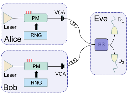
Figure 1: Schematic of phase-matching QKD without intensity modulation. Alice and Bob utilize pulse laser sources to prepare weak coherent states. They use a random number generator (RNG) to generate random numbers for random phases and random key bits. For each pulse train, Alice and Bob exploit a phase modulator (PM) to apply phase $\theta_{a}+r_{a}\pi$ and $\theta_{b}+r_{b}\pi$ on each pulse according to the random phase selection and random key bits $r_{a}$ and $r_{b}\in\{0,1\}$, respectively. A variable optical attenuator (VOA) is used to implement a weak pulse with single-photon-level modulation. An untrusted Eve receives the two pulses from Alice and Bob and then uses a beam splitter (BS) and single-photon detectors to conduct an interference measurement.

2. Measurement. Eve uses the two pulses from Alice and Bob to conduct an interference measurement and chooses a single detector ($D_{1}$ or $D_{2}$) click as a valid click.

3. Sifting. After measurement, Eve announces the clicking detector when a valid click occurs. Then, Alice and Bob announce their corresponding random phases. They will keep the data if $|\theta_{a}-\theta_{b}|$ = 0 or $\pi$. If detector $D_{2}$ clicks and $|\theta_{a}-\theta_{b}|$ = 0 (if $D_{1}$ clicks and $|\theta_{a}-\theta_{b}|$ = $\pi$), Bob will flip his bit. Steps 1 to 3 are repeated $N$ times until the data is sufficient to conduct the steps below.

4. Parameter estimation. Alice randomly samples some data with probability $p_{s}$ as the test data and announces the locations and bits information. Bob calculates the bit error number $m_{s}$ of test data and announces to Alice. The rest of the data serve as the shift key.

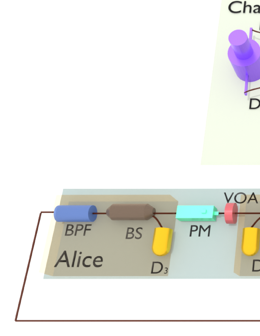
Figure 2: Schematic of the proof-of-principle experiment. Detectors $D_{1}$ and $D_{2}$ are superconductor nanowire single-photon detectors. Detectors $D_{3}$, $D_{4}$, $D_{5}$, and $D_{6}$, which monitor the intensity of pulses, are photodiodes. All the devices are synchronized by the signals from an arbitrary waveform generator. The pulses are emitted from a homemade laser and reach a circulator (Cir) whose direction is from 1 to 2 and from 2 to 3.

Then, the pulse is separated into two pulses by a 50:50 BS, and the two pulses enter a Sagnac loop. Before modulation, the pulse passes through a bandpass filter (BPF) and the BS. Alice and Bob can distinguish whether a pulse belongs to them after time calibration. The two pulses modulated by Alice and Bob passing through the Sagnac loop will interfere with each other by the BS. Polarization controllers (PCs) modify the polarization of the two pulses to maximize the detection efficiencies. Finally, the pulses after interference are then detected by two single-photon detectors $D_{1}$ and $D_{2}$. Note that the devices covered with the yellow cuboid are not introduced in the implementation.

5. Postprocessing. Finally, Alice and Bob conduct error correction and privacy amplification. After that, Alice and Bob obtain the final secret keys.

The differences between our protocol and conventional phase-matching QKD [36] can be summarized as follows. Firstly, our protocol eliminates the requirement for intensity modulation, thereby avoiding the pattern effect associated with it. Secondly, our protocol utilizes fewer phase slices compared to conventional phase-matching QKD due to the lower intensity.

III Experimental Demonstration

To demonstrate the feasibility of our protocol, we implement a proof-of-principle experiment. The experimental setup is shown in Fig. 2. We exploit a Sagnac loop to stabilize the fluctuation of the phase caused by the path [82].

The laser source is held by the third party, Charlie. The frequency of the pulse laser is set as 100 MHz, and the duty cycle is less than $3\%$. Charlie utilizes the laser to generate pulses sent to Alice and Bob. The pulses pass through a circulator (Cir) and a 50:50 BS whose port numbers are shown in Fig. 2. Then, the two identical pulses will enter the loop. Alice and Bob capture and modulate their own pulses. The rule of modulating the corresponding pulses is as following: Alice modulates the clockwise pulse, and Bob modulates the counterclockwise pulse. In the loop, we utilize four BPFs for filtering and four BSs and detectors to monitor the injected pulse intensities. We did not realize pulse filtering and intensity monitoring because of the device limitations. The impact on the results caused by the lacking devices is too slight to consider. As mentioned above, different random phases are generated with an equal probability 12.5%, and key are selected with a probability 50%. Therefore, we used Python to generate a set of random numbers for the arbitrary waveform generator (Tabor Electronics, P2588B). In our implementation, we select eight slices of the random phase, which is more complex than the six slices in experiment, and the length of the random number is 10000. Then, the radio-frequency signals are amplified by an electrical driver to drive the PM to modulate the total phase. The pulses modulated by Alice and Bob pass through the VOA and different BS ports to the detection units. After interference at the BS, the pulses are detected by $D_{1}$ and $D_{2}$. For $D_{1}$, the detection efficiency is 86.3% and the dark count rate is 13.1 Hz. For $D_{2}$, the detection efficiency is 82.9% and the dark count rate is 18.9 Hz. The losses of Charlie’s components are presented in Table LABEL:EFF_OPT at the end. The length of the time window is 1.8 ns. We ran the system for 1000 seconds under different channel losses to accumulate sufficient detection events and distilled the raw keys.

IV Security Analysis

For phase-matching QKD [36], the phase error rate is only related to the even-photon component [41, 45]. Strictly, for security proofs based on photon-number states, continuous phase randomization is required. We use a discrete phase randomization ($M=6,8$) to replace continuous phase randomization to enhance the accessibility. Initially, we calculate the phase error rate for the case of continuous phase randomization. Then, we analyze the deviation that occurs in our protocol when employing discrete modulations. Based on the analysis, the discrete random phase can be used to replace the continuous random phase even if $M$ is 6 or 8.

IV.1 Continuous-phase randomization

After the continuous-phase randomization, the joint system between Alice’s and Bob’s can be regarded as a mixture of photon-number states

$$\rho_{ab} =\frac{1}{2\pi}\int_{0}^{2\pi}|\mu e^{i\theta}\rangle_{ab}\langle\mu e^{i\theta}|d\theta$$ (1)

$$=\sum_{k=0}^{\infty}P_{k}|k\rangle_{ab}\langle k|,$$

where we have the probability of joint $k$-photon $P_{k}=e^{-\mu}\mu^{k}/k!$ and $k$ is the joint photon number between Alice and Bob. The phase error rate can be written as [41, 45]

$$E_{p}=\sum_{k=0}^{\infty}q_{2k}=\frac{1}{Q_{\mu}}\sum_{k=0}^{\infty}P_{2k}Y_{2k},$$ (2)

where $q_{k}=P_{k}Y_{k}/Q_{\mu}$ is the ratio of joint $k$-photon in the final valid detection event. $Q_{\mu}$ is the gain of Alice and Bob sends optical pulses with intensities $\mu_{a}$ and $\mu_{b}=\mu-\mu_{a}$, respectively. $Y_{k}$ is the yield of joint $k$-photon between Alice and Bob ( $0\leq Y_{k}\leq 1$).

To estimate the yield of vacuum state $Y_{0}$, one needs to randomly sample some bits to obtain the QBER. The observed value of the sampled bit error number is $m_{s}$. Then, we use the variant of the Chernoff bound [83] to estimate the expected upper bound of the sampled bit error number $\overline{m}_{s}^{*}=\phi^{U}(m_{s})$, where $\phi^{U}(x)=x+\beta+\sqrt{2\beta x+\beta^{2}}$, $\beta=\rm{log}(\epsilon^{-1})$ and $\epsilon$ is the failure probability. Therefore, the upper bound of the expected bit error number $m^{*}$ in the shift key can be given by

$$\overline{m}^{*}=\frac{(1-p_{s})}{p_{s}}\overline{m}_{s}^{*}.$$ (3)

The expected value of error data number $\overline{m}_{0}^{*}$ caused by vacuum state is not greater than the total error data number $\overline{m}^{*}$, namely, $\overline{m}_{0}^{*}\leq\overline{m}^{*}$. A useful observation is that zero photon will result in half the expected error detection data, i.e., $\overline{n}_{0}^{*}=2\overline{m}_{0}^{*}$ and $n_{0}^{*}$ is the expected value of vacuum state’s contribution. Therefore, the upper bound of $Y_{0}$ can be given by

$$\overline{Y}_{0}=\frac{\overline{n}_{0}}{N(1-p_{s})e^{-\mu}},$$ (4)

where the observed value $\overline{n}_{0}=\Phi(\overline{n}_{0}^{*})$ is calculated by the Chernoff bound [83] $\Phi^{U}(x)=x+\beta/2+\sqrt{2\beta x+\beta^{2}/4}$.

Combining the discussion above, we incorporate the upper bound of observed value of $\overline{Y}_{0}$ and probability distribution $P_{2k}$ into the formula of phase error rate

$$E_{p} =\frac{1}{Q_{\mu}}P_{0}Y_{0}+\frac{1}{Q_{\mu}}\sum_{k=1}^{\infty}P_{2k}Y_{2k}$$ (5)

$$\leq\frac{1}{Q_{\mu}}P_{0}Y_{0}+\frac{1}{Q_{\mu}}\sum_{k=1}^{\infty}P_{2k}$$

$$\leq\frac{e^{-\mu}\overline{Y}_{0}}{Q_{\mu}}+\frac{e^{-2\mu}+1-2e^{-\mu}}{2Q_{\mu}}.$$

For the purpose of estimating the upper bound of the phase error rate, we set the worst case that $Y_{2k}=1$ with $k\geq 1$ considering the negligible $P_{2k}$ at the second line of Eq. (5).

IV.2 Discrete-phase randomization

For the case of discrete random phase modulation, the system will become a group of “pseudo” Fock states according to the density matrix of the states that Alice and Bob prepare [84]

$$\frac{1}{M}\sum_{j=0}^{M-1}|\sqrt{\mu}e^{i\theta_{j}}\rangle\langle\sqrt{\mu}e^{i\theta_{j}}|=\sum_{k=0}^{M-1}P^{\mu}_{M}(k)|\lambda_{k}\rangle\langle\lambda_{k}|,$$ (6)

where

$$|\lambda_{k}\rangle=\frac{e^{-\mu/2}}{\sqrt{P^{\mu}_{M}(k)}}\sum_{l=0}^{\infty}\frac{(\sqrt{\mu})^{lM+k}}{\sqrt{(lM+k)!}}|lM+k\rangle,$$ (7)

and

$$P^{\mu}_{M}(k)=\sum_{l=0}^{\infty}\frac{(\mu)^{lM+k}e^{-\mu}}{(lM+k)!}.$$ (8)

Observing this form, the state becomes the Fock state when the $M$ is large enough. If $M$ is even, each pesudo even Fock state $\left|\lambda_{k}\right\rangle$ contains only even photon-number states. Based on the phase-matching QKD protocol analysis [41, 45], the phase error rate is contributed only by the even-photon components. Therefore, we can consider only the deviation of even-photon component when the random phase slices $M=8$. The pesudo even photon numbers are $\{0,2,4,6\}$. Furthermore, we test the $M=6$ and the pesudo even numbers are taken as $\{0,2,4\}$. The even-photon deviation is shown below [45], and more details are presented in Appendix A

$$\delta_{k}=|q_{k}-q_{k}^{M}|\leq\frac{P^{\mu}_{M}(k)}{Q_{\mu}}\sqrt{\frac{k!\mu^{M}}{(M+k)!}}.$$ (9)

From Eq. (2), the deviation will cause the extra phase error rate. We could write the total phase error rate with $M$-slice random phase

$$E_{p}^{M} =\sum_{k=0}^{M/2-1}q_{2k}^{M}$$ (10)

$$\leq\frac{e^{-\mu}\overline{Y}_{0}}{Q_{\mu}}+\frac{e^{-2\mu}+1-2e^{-\mu}}{2Q_{\mu}}+\sum_{k=0}^{M/2-1}\delta_{2k}.$$

The detailed derivation of this problem has been carried out in Appendix B. Furthermore, we use the Kato inequality [85] to defend against the coherent attacks for the dependent random variables. Further details regarding this approach are provided in Appendix C.

V Simulation Results

Let us define $\xi^{\prime}$ as the bits consumed to ensure that the failure probability of error verification reaches $2^{-\xi^{\prime}}$, and $\xi$ denotes the additional amount of privacy amplification to further enhance the privacy. According to complementarity [15, 43], an $\epsilon_{\rm sec}$ -secret and $\epsilon_{\rm cor}$-correct key of length is

$$\ell=n_{\mu}[1-H(\overline{E}_{p}^{M})-fH(E_{b})]-\xi-\xi^{\prime},$$ (11)

where $n_{\mu}=\frac{2}{M}Q_{\mu}N(1-p_{s})$ is the remaining bit number to generate the logic bits, $H(x)=-x{\rm log_{2}}x-(1-x){\rm log_{2}}(1-x)$ is the Shannon entropy function, $E_{b}=e_{d}(1-p_{d})[1-(1-p_{d})e^{-\mu\eta}]/Q_{\mu}+(1-e_{d})p_{d}(1-p_{d})e^{-\mu\eta}/Q_{\mu}$ is the QBER, and $\overline{E}_{p}^{M}$ is the total phase error rate with phase slice number $M$ after applying Kato inequality to defend against the coherent attacks. The total gain $Q_{\mu}=(1-p_{d})[1-(1-2p_{d})e^{-\mu\eta}]$.

Table I: Simulation parameters [86]. The misalignment error and dark count rate are denoted by $e_{d}$ and $p_{d}$, respectively. $f$ is the error correction efficiency, $\eta_{d}$ is the detector efficiency, $\alpha$ is the loss coefficient, and $M$ is the number of phase slices whose value will influence the even-photon deviation.

$e_{d}$	$p_{d}$	$f$	$\eta_{d}$	$\alpha$	$M$
0.01	$10^{-8}$	1.16	56%	0.168	6 or 8

Due to the application of the Chernoff bound twice, the security parameters can be expressed as $\epsilon_{\rm sec}=\sqrt{2}\sqrt{2\epsilon+2^{-\xi}}$ and $\epsilon_{\rm cor}=2^{-\xi^{\prime}}$. Furthermore, we utilize the Kato inequality to defend against the coherent attacks for the dependent random variables. The $\epsilon_{\rm{Ka}}$ is the failure probability in Kato inequality. Therefore, the final security parameter is $\epsilon_{\rm tot}=\epsilon_{\rm sec}+\epsilon_{\rm cor}+\epsilon_{\rm{Ka}}=\sqrt{2}\sqrt{2\epsilon+2^{-\xi}}+2^{-\xi^{\prime}}+\epsilon_{\rm{Ka}}$. In the simulation, we set $\epsilon_{\rm sec}=2\times 10^{-10}$, $\epsilon_{\rm cor}=10^{-15}$ and $\epsilon_{\rm{Ka}}=10^{-10}$. We can conclude that $\epsilon=10^{-20}/2$, $\xi=\rm{log}_{2}(2/10^{-20})$, $\xi^{\prime}=\rm{log}_{2}(1/10^{-15})$ and $\epsilon_{\rm tot}=3\times 10^{-10}$.

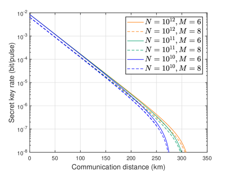
Figure 3: Finite-size simulation results of our protocol. The parameters are shown in Table LABEL:parameter. We select data sizes $N=10^{10}$, $10^{11}$, and $10^{12}$ to conduct the simulation.

Here, we numerically simulate the key rate $R=\ell/N$ of our protocol in finite-size cases. The other parameter settings are shown in Table LABEL:parameter. The finite-size simulation results are shown in Fig. 3.

Our protocol achieves a 305-km transmission distance with $N=10^{12}$. At the condition of $N=10^{11}$, the transmission distance can reach 298 km with the $10^{-8}$ key rate. Even when the data size is not a large number, such as $10^{10}$, the transmission distance reaches 270 km.

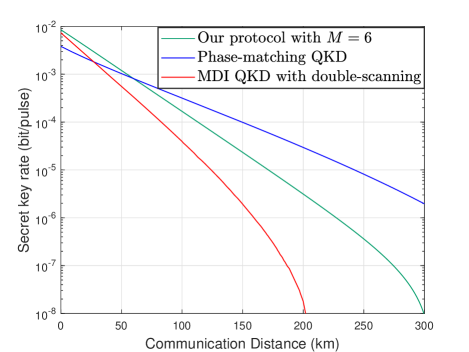
Figure 4: We compare the performance of our protocol with phase-matching QKD [36] and four-intensity MDI QKD using the double-scanning method [87]. The simulation parameters are provided in Table LABEL:parameter with a data size of $N=10^{11}$. The phase slice number of our protocol $M$ is set as 6 in comparison. The total security parameter $\epsilon_{\rm{tot}}$ of four-intensity MDI QKD using the double-scanning method is the same for that of our protocol, which is equal to $3\times 10^{-10}$.

From Fig. 4, we can observe that our protocol demonstrates superior performance within a 60-km range, and the key rate achieved by our protocol is comparable to that of phase-matching QKD at a distance of 100 km. This implies that our protocol achieves a similar key rate to phase-matching QKD in metropolitan areas without the need for intensity modulation. Compared to four-intensity MDI QKD with double-scanning method, our protocol demonstrates a key rate advantage of approximately 4 times at a distance of 100 km.

QKD focuses on applicability and security rather than the only transmission distance. In the case of intercity communication where the distance is 500 km or more, the key rate is too low to be practically applicable. However, within metropolitan areas, such as in 100-km distance communication which is the main field of application. In such a situation, our protocol achieves a key rate comparable to that of phase-matching QKD while overcoming the pattern effect and simplifying experimental requirements. It is worthwhile to note that phase-matching QKD and four-intensity MDI QKD using the double-scanning method require perfect intensity modulation, which is impractical in experiments. Additionally, the pattern effect in these methods leaks information to potential eavesdroppers. These issues [69, 66] significantly decrease the key rate of phase-matching QKD and four-intensity MDI QKD with double-scanning method, further highlighting the competitiveness of our protocol.

The change in the deviation with attenuation is shown in Fig. 5. We find that the influence of the deviation is too small to consider. From Eq. (10), the deviation has such a negligible effect on the phase error rate that it can be disregarded, and the phase error rate increases by less than $1\%$ of itself when using 6-slice random phase. The substitution of fewer slices does not invalidate the security proof that relies on photon-number states. In some extreme circumstances, such as with a high source intensity, we have to utilize more slices to achieve the replacement, but this comes at the expense of some key rate and experimental complexity. Because the intensity of the pulse we use is sufficiently low, we can use a small number of phase slices, which is set as 6 or 8 in our protocol, to replace the continuous random phase.

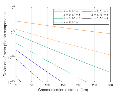
Figure 5: Deviation of the even-photon state in our protocol. We simulate the deviation with the data size $N=10^{11}$. The other parameters chosen are shown in Table LABEL:parameter. The deviation of the even-photon state can denote the gap between the continuous random phase and discrete random phase.

VI Experimental Results

Table II: Summary of experimental data. We tested the key rate under different channel losses. The table shows the data size $N$, the total intensity of pulses $\mu$, experimental QBER $E_{b}$, number of the remaining bits $n_{\mu}$, and key rate $R$. Note that losses of 35, 40, and 45 dB correspond to $p_{s}$ of $7\%$.

Loss	$N$	$\mu$	$E_{b}$	$n_{\mu}$	$R$
35 dB	$10^{11}$	3.20$\times 10^{-3}$	0.22%	934403	3.00$\times 10^{-6}$
40 dB	$10^{11}$	1.87$\times 10^{-3}$	0.33%	302187	8.50$\times 10^{-7}$
45 dB	$10^{11}$	9.78$\times 10^{-4}$	0.71%	91781	2.25$\times 10^{-7}$

We implement a proof-of-principle experiment to test our protocol under 35-, 40-, and 45-dB channel losses with the experimental setup depicted in Fig. 2. The experimental results we obtained are listed in Table II and Fig. 6.

We implement experiments and obtain the total detection counts and total QBER $E_{b}$ under the total intensity $\mu$ with $N=10^{11}$. The optimized pulse intensity is acquired by using the genetic algorithm in simulations with different channel losses. Given the 100-MHz repetition rate, our protocol can obtain a secure key rate of 22.5 bit/s when the channel loss is over 45 dB, which means that it can be implemented over 267 km with existing technologies. A secure key rate of 0.3 kbit/s is generated at 35 dB ($\sim$208 km), while at 40 dB ($\sim$238 km), the rate is 85 bit/s. The more details of experiment is shown in Appendix D.

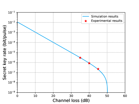
Figure 6: Considering the experimental results, we depict the secret key rate when the data size $N=10^{11}$ and phase slice $M=8$. We implement the experiment with the optimized intensity under 35 dB, 40 dB and 45 dB channel losses.

As a proof-of-principle demonstration, the aim of implementing the scheme is to verify the feasibility of our protocol instead of establishing a complete system. We used the Sagnac loop to stabilize the phase automatically, and thus, the pulses modulated by the two users were generated by a third party, which resulted in security flaws. For real optical fiber implementation, our protocol can be performed by using the phase locking and phase tracking method to replace the Sagnac loop, where two users are independent.

VII Conclusion

In this work, we propose a phase-matching QKD protocol without intensity modulation. Since the need of sending decoy states to calculate the secret key rate is removed, our protocol avoids the pulse correlation resulting from multi-intensity modulation and simplifies the experimental requirements. A alternative estimation method is introduced to obtain the phase error rate in our security analysis, which assumes that the vacuum state contributes to the whole QBER in order to obtain an upper bound on the vacuum state phase error rate.

We utilize the Kato inequality to defend against the coherent attacks for the dependent random variables. Based on these considerations, we conducted a simulation to demonstrate the key rate of our protocol. Simulation results show that our protocol can reach 305 km with a data size of $N=10^{12}$. Our protocol demonstrates a advantage of approximately 4 times the magnitude in the key rate compared to the four-intensity MDI QKD with the double-scanning method at 100 km. Furthermore, within metropolitan areas, our protocol achieves a comparable key rate to that of phase-matching QKD. Considering the imperfect intensity modulation and its pattern effect, our protocol becomes even more competitive. The feasibility of using discrete random phase with fewer phase slices (M = 6, 8) has been demonstrated by the simulation results. With low pulse intensity, we need only a six-slice or eight-slice random phases, which further reduces the experimental complexity and saves the random number resources. A proof-of-principle experiment is implemented to demonstrate the feasibility of our protocol, and the experimental results shows that our protocol can achieve a key rate of 22.5 bit/s under a 45 dB channel loss. The experimental results are consistent with the simulation results. The simplicity and efficiency of our protocol, achieved through the avoidance of intensity modulation and the use of fewer slice random phases, make it a practical solution for quantum communication.

Appendix A Deviation of even-photon components

The following derivation is based on Ref. [45]. Note that $P^{\mu}_{M}(k)\geq P_{k}$, the deviation of even-photon components can be bounded by

$$|q_{k}-q_{k}^{M}| =\frac{|Y_{k}P_{k}-Y_{k}^{M}P^{\mu}_{M}(k)|}{Q_{\mu}}$$ (A1)

$$\leq P^{\mu}_{M}(k)\frac{|Y_{k}-Y_{k}^{M}|}{Q_{\mu}},$$

where $Y_{k}^{M}$ is the yield of joint $k$-photon with $M$-slice random phase. The deviation of yield is bounded with $|Y_{k}-Y_{k}^{M}|\leq\sqrt{1-|\langle k|\lambda_{k}\rangle|^{2}}$. Further, we get

$$|\langle k|\lambda_{k}\rangle|^{2} =\frac{e^{-\mu}}{P^{\mu}_{M}(k)}\left|\sum_{l=0}^{\infty}\frac{(\sqrt{\mu})^{lM+k}}{\sqrt{(lM+k)!}}\langle k|lM+k\rangle\right|^{2}$$ (A2)

$$=\frac{e^{-\mu}\mu^{k}}{P^{\mu}_{M}(k)k!}$$

$$=\frac{1}{\left(\sum_{l=0}^{\infty}\frac{k!}{(lM+k)!}\mu^{lM}\right)}.$$

Here, we take an inequality $[(l+1)M+k]!\geq[(lM)+k]!(M+k)!/k!$ into the formula above

$$|\langle k|\lambda_{k}\rangle|^{2} \geq\frac{1}{\sum_{l=0}^{\infty}\left(\frac{k!}{(M+k)!}\mu^{M}\right)^{l}}$$ (A3)

$$=1-\frac{k!}{(M+k)!}\mu^{M}.$$

Then, we take the formula into the bound of even-photon deviation

$$|q_{k}-q_{k}^{M}| \leq\frac{P^{\mu}_{M}(k)}{Q_{\mu}}\sqrt{\frac{k!\mu^{M}}{(M+k)!}},$$ (A4)

when $M\geq 2$, the inequality is always satisfied. For k=0, we have

$$P^{\mu}_{M}(0) =\sum_{l=0}^{\infty}\frac{(\mu)^{lM}e^{-\mu}}{(lM)!}$$ (A5)

$$\leq\sum_{l=0}^{\infty}\frac{(\mu)^{2l}e^{-\mu}}{(2l)!}$$

$$=\frac{1+e^{-2\mu}}{2}.$$

For ${k=2}$, we have

$$P^{\mu}_{M}(2) \leq\sum_{l=1}^{\infty}\frac{(\mu)^{2l}e^{-\mu}}{(2l)!}$$ (A6)

$$=\frac{1}{2}(1+e^{-2\mu}-2e^{-\mu}).$$

For ${k=4}$

$$P^{\mu}_{M}(4) \leq\sum_{l=2}^{\infty}\frac{(\mu)^{2l}e^{-\mu}}{(2l)!}$$ (A7)

$$=\frac{1+e^{-2\mu}-2e^{-\mu}-\mu^{2}e^{-\mu}}{2}.$$

For ${k=6}$, we have

$$P^{\mu}_{M}(6) \leq\sum_{l=3}^{\infty}\frac{(\mu)^{2l}e^{-\mu}}{(2l)!}$$ (A8)

$$=\frac{1+e^{-2\mu}-2e^{-\mu}-\mu^{2}e^{-\mu}-2\mu^{4}e^{-\mu}/4!}{2}.$$

Taking the formula above into Eq. (9), we could get the deviation of even-photon components and total phase error rate with $M$ phase slices $E_{p}^{M}$.

Table III: Experimental data.

Channel loss	35 dB		40 dB		45 dB
$n_{\rm{det}}$	3701806		1196818		363094
Detector	$D_{1}$	$D_{2}$	$D_{1}$	$D_{2}$	$D_{1}$	$D_{2}$
Detected 00	46871	191	15320	88	4669	40
Detected $\frac{\pi}{4}\frac{\pi}{4}$	49260	93	15749	49	4835	42
Detected $\frac{\pi}{2}\frac{\pi}{2}$	48173	71	15602	42	4716	45
Detected $\frac{3\pi}{4}\frac{3\pi}{4}$	46155	156	14682	74	4573	42
Detected $\pi\pi$	46633	180	15041	82	4552	48
Detected $\frac{5\pi}{4}\frac{5\pi}{4}$	45777	123	14696	64	4448	53
Detected $\frac{3\pi}{2}\frac{3\pi}{2}$	44793	84	14432	53	4409	39
Detected $\frac{7\pi}{4}\frac{7\pi}{4}$	51171	151	16537	76	5029	57
Detected $0\pi$	160	72580	78	23467	44	6940
Detected $\frac{\pi}{4}\frac{5\pi}{4}$	75	68516	47	21991	28	6747
Detected $\frac{\pi}{2}\frac{3\pi}{2}$	65	69200	46	22609	38	6681
Detected $\frac{3\pi}{4}\frac{7\pi}{4}$	159	70182	64	22637	34	6878
Detected $\pi 0$	162	70496	60	22976	35	6805
Detected $\frac{5\pi}{4}\frac{\pi}{4}$	136	73887	67	23511	43	7292
Detected $\frac{3\pi}{2}\frac{\pi}{2}$	89	67507	45	22036	31	6539
Detected $\frac{7\pi}{4}\frac{3\pi}{4}$	131	62112	64	20205	30	6019

Appendix B Phase error rate derivation details of discrete random phase

For more clarity, we give the phase error rate derivation details of discrete random phase. As Eq. (2) shows, we give a discrete version of phase error rate

$$E_{p}^{M} =\sum_{k=0}^{M/2-1}q_{2k}^{M}$$ (B9)

$$\leq\sum_{k=0}^{M/2-1}q_{2k}+\delta_{2k}$$

$$\leq\sum_{k=0}^{\infty}q_{2k}+\sum_{k=0}^{M/2-1}\delta_{2k},$$

the first inequality is obtained from Eq. (9), and we expand the $q_{2k}$ sum range of the $k$ from $M/2-1$ to $\infty$ to get the second inequality. Combining with Eqs. (2) and (5), the phase error rate can be written as

$$E_{p}^{M}\leq\frac{e^{-\mu}\overline{Y}_{0}}{Q_{\mu}}+\frac{e^{-2\mu}+1-2e^{-\mu}}{2Q_{\mu}}+\sum_{k=0}^{M/2-1}\delta_{2k}.$$ (B10)

Appendix C Utilizing Kato inequality to defend against the coherent attacks

With the analysis of deviation between the continuous and discrete random phase [45], our protocol applies only to the collective attacks for Eq. (A1). Here, we incorporate the Kato inequality [85], which allows us to defend against coherent attacks for dependent random variables. The Kato inequality offers a tighter bound compared to the commonly used Azuma inequality [88].

Let us consider a sequence of Bernoulli random variables denoted as $\chi_{1},...,\chi_{n}$, and define $\Lambda_{j}$ as the sum of these random variables, i.e., $\Lambda_{j}=\sum_{u=1}^{j}\chi_{u}$. We also introduce $\mathcal{F}j$ as the $\sigma$-algebra generated by ${\chi_{1},...,\chi_{n}}$, representing the natural filtration of these Bernoulli random variables. Furthermore, let $\epsilon_{\rm{Ka}}$ represent the failure probabilities associated with the Kato inequality bound for sums of dependent random variables. By utilizing the findings presented in Refs. [88, 85], we could find that

$${\rm Pr}\left[\sum\limits_{u=1}^{n}{\rm Pr}(\xi_{u}=1|\mathcal{F}_{u-1})-\Lambda_{n}\geq(b+a\left(\frac{2\Lambda_{n}}{n}-1\right))\sqrt{n}\right]$$ (C11)

$$\leq{\rm exp}\left[\frac{-2(b^{2}-a^{2})}{1+\frac{4a}{3\sqrt{n}}}\right],$$

by equating the right-hand sides of Eq. (C11) to $\epsilon_{\rm{Ka}}$ and solving for $a$ and $b$, a tighter bound was derived [88]. This improved bound can be formulated as

$$\sum\limits_{u=1}^{n}{\rm Pr}(\chi_{u}=1|\chi_{1},...,\chi_{u-1})\leq\Lambda_{n}+\Delta_{\rm{Ka}}(n,\Lambda_{n},\epsilon_{\rm{Ka}}),$$ (C12)

where $\Delta_{\rm{Ka}}(n,\Lambda_{n},\epsilon_{\rm{Ka}})=\left[b+a(\frac{2\Lambda_{n}}{n}-1)\right]\sqrt{n}$, where the $b$ and $a$ is set as

$$a=\frac{3\left[72\sqrt{n}\Lambda_{n}(n-\Lambda_{n}){\rm ln}\epsilon_{\rm{Ka}}-16(n)^{3/2}{\rm ln}^{2}\epsilon_{\rm{Ka}}+9\sqrt{2}(n-2\Lambda_{n})a_{1}\right]}{4(9n-8{\rm ln}\epsilon_{\rm{Ka}})[9\Lambda_{n}(n-\Lambda_{n})-2n{\rm ln}\epsilon_{\rm{Ka}}]},$$ (C13)

$$b=\frac{\sqrt{18a^{2}n-(16a^{2}+24a\sqrt{n}+9n){\rm ln}\epsilon_{\rm{Ka}}}}{3\sqrt{2n}},$$

where $a_{1}=\sqrt{-n^{2}{\rm ln}\epsilon_{\rm{Ka}}[9\Lambda_{n}(n-\Lambda_{n})-2n{\rm ln}\epsilon_{\rm{Ka}}]}$, and $\epsilon_{\rm{Ka}}$ represents the maximum failure probability among the bounds mentioned in Eq. (C12). To estimate the upper bound of the phase error rate using the Kato inequality, we need to make a prediction of $\Lambda_{n}$, denoted as $\overline{\Lambda}_{n}$. This prediction is obtained during our security analysis process.

Considering the Kato inequality and the former phase error rate with finite-size analysis we obtain, the final phase error rate can be given by

$$\overline{E}_{p}^{M}\leq\frac{n_{\mu}E_{p}^{M}+\Delta_{\rm{Ka}}(n_{\mu},n_{\mu}E_{p}^{M},\epsilon_{\rm{Ka}})}{n_{\mu}}.$$ (C14)

Appendix D Experimental details

Table IV: Efficiencies of devices in the measurement station.

Optical devices	Attenuation
Cir 2$\rightarrow$3	0.77 dB
BS-3-1	3.61 dB
BS-3-2	3.58 dB
BS-4-1	3.80 dB
BS-4-2	3.81 dB
$PC_{1}$	0.18 dB
$PC_{2}$	0.16 dB

The experimental results are summarized in Table LABEL:EXP_DET, including the number of all detection events $n_{\rm{det}}$ and the number of detection events under different added phases. We denote the number of detection events under different added phases as “Detected AB”, where “A” (“B”) means that adding an A (B) phase to the pulse by Alice (Bob). The optical transmittance of the elements at Charlie’s site are listed in Table LABEL:EFF_OPT. The elements include the PM, PCs, Cir, and BS. The results of each channel are given accordingly. From the elements, we can obtain the proper additional loss to reach the total channel loss we need.

References

- Bennett and Brassard [2014] C. H. Bennett and G. Brassard, Quantum cryptography: Public key distribution and coin tossing, Theor. Comput. Sci. 560, 7 (2014).
- Ekert [1991] A. K. Ekert, Quantum cryptography based on bell’s theorem, Phys. Rev. Lett. 67, 661 (1991).
- Bennett et al. [1992] C. H. Bennett, G. Brassard, and N. D. Mermin, Quantum cryptography without bell’s theorem, Phys. Rev. Lett. 68, 557 (1992).
- Arute et al. [2019] F. Arute, K. Arya, R. Babbush, D. Bacon, J. C. Bardin, R. Barends, R. Biswas, S. Boixo, F. G. Brandao, D. A. Buell, et al., Quantum supremacy using a programmable superconducting processor, Nature 574, 505 (2019).
- Zhong et al. [2020] H.-S. Zhong, H. Wang, Y.-H. Deng, M.-C. Chen, L.-C. Peng, Y.-H. Luo, J. Qin, D. Wu, X. Ding, Y. Hu, et al., Quantum computational advantage using photons, Science 370, 1460 (2020).
- Yin et al. [2023] H.-L. Yin, Y. Fu, C.-L. Li, C.-X. Weng, B.-H. Li, J. Gu, Y.-S. Lu, S. Huang, and Z.-B. Chen, Experimental quantum secure network with digital signatures and encryption, Natl. Sci. Rev. 10, nwac228 (2023).
- Biamonte et al. [2017] J. Biamonte, P. Wittek, N. Pancotti, P. Rebentrost, N. Wiebe, and S. Lloyd, Quantum machine learning, Nature 549, 195 (2017).
- Xie et al. [2021] Y.-M. Xie, B.-H. Li, Y.-S. Lu, X.-Y. Cao, W.-B. Liu, H.-L. Yin, and Z.-B. Chen, Overcoming the rate–distance limit of device-independent quantum key distribution, Opt. Lett. 46, 1632 (2021).
- Zhou et al. [2022] M.-G. Zhou, X.-Y. Cao, Y.-S. Lu, Y. Wang, Y. Bao, Z.-Y. Jia, Y. Fu, H.-L. Yin, and Z.-B. Chen, Experimental quantum advantage with quantum coupon collector, Research 2022, 9798679 (2022).
- Bennett [1992] C. H. Bennett, Quantum cryptography using any two nonorthogonal states, Phys. Rev. Lett. 68, 3121 (1992).
- Bruß [1998] D. Bruß, Optimal eavesdropping in quantum cryptography with six states, Phys. Rev. Lett. 81, 3018 (1998).
- Koashi and Preskill [2003] M. Koashi and J. Preskill, Secure quantum key distribution with an uncharacterized source, Phys. Rev. Lett. 90, 057902 (2003).
- Kraus et al. [2005] B. Kraus, N. Gisin, and R. Renner, Lower and upper bounds on the secret-key rate for quantum key distribution protocols using one-way classical communication, Phys. Rev. Lett. 95, 080501 (2005).
- Renner [2008] R. Renner, Security of quantum key distribution, Int. J. Quantum. Inf. 6, 1 (2008).
- Koashi [2009] M. Koashi, Simple security proof of quantum key distribution based on complementarity, New J. Phys. 11, 045018 (2009).
- Tomamichel and Renner [2011] M. Tomamichel and R. Renner, Uncertainty relation for smooth entropies, Phys. Rev. Lett. 106, 110506 (2011).
- Weedbrook et al. [2012] C. Weedbrook, S. Pirandola, R. García-Patrón, N. J. Cerf, T. C. Ralph, J. H. Shapiro, and S. Lloyd, Gaussian quantum information, Rev. Mod. Phys. 84, 621 (2012).
- Xu et al. [2020] F. Xu, X. Ma, Q. Zhang, H.-K. Lo, and J.-W. Pan, Secure quantum key distribution with realistic devices, Rev. Mod. Phys. 92, 025002 (2020).
- Liu et al. [2021] W.-B. Liu, C.-L. Li, Y.-M. Xie, C.-X. Weng, J. Gu, X.-Y. Cao, Y.-S. Lu, B.-H. Li, H.-L. Yin, and Z.-B. Chen, Homodyne detection quadrature phase shift keying continuous-variable quantum key distribution with high excess noise tolerance, PRX Quantum 2, 040334 (2021).
- Xu et al. [2010] F. Xu, B. Qi, and H.-K. Lo, Experimental demonstration of phase-remapping attack in a practical quantum key distribution system, New J. Phys. 12, 113026 (2010).
- Lydersen et al. [2010] L. Lydersen, J. Skaar, V. Makarov, C. Wiechers, C. Wittmann, and D. Elser, Hacking commercial quantum cryptography systems by tailored bright illumination, Nat. Photonics 4, 686 (2010).
- Tang et al. [2013] Y.-L. Tang, H.-L. Yin, X. Ma, C.-H. F. Fung, Y. Liu, H.-L. Yong, T.-Y. Chen, C.-Z. Peng, Z.-B. Chen, and J.-W. Pan, Source attack of decoy-state quantum key distribution using phase information, Phys. Rev. A 88, 022308 (2013).
- Xu et al. [2015] F. Xu, K. Wei, S. Sajeed, S. Kaiser, S. Sun, Z. Tang, L. Qian, V. Makarov, and H.-K. Lo, Experimental quantum key distribution with source flaws, Phys. Rev. A 92, 032305 (2015).
- Pereira et al. [2019] M. Pereira, M. Curty, and K. Tamaki, Quantum key distribution with flawed and leaky sources, npj Quantum Inf. 5, 62 (2019).
- Huang et al. [2019] A. Huang, A. Navarrete, S.-H. Sun, P. Chaiwongkhot, M. Curty, and V. Makarov, Laser-seeding attack in quantum key distribution, Phys. Rev. Applied 12, 064043 (2019).
- Huang et al. [2023] A. Huang, A. Mizutani, H.-K. Lo, V. Makarov, and K. Tamaki, Characterization of state-preparation uncertainty in quantum key distribution, Phys. Rev. Applied 19, 014048 (2023).
- Lo et al. [2012] H.-K. Lo, M. Curty, and B. Qi, Measurement-device-independent quantum key distribution, Phys. Rev. Lett. 108, 130503 (2012).
- Comandar et al. [2016] L. C. Comandar, M. Lucamarini, B. Fröhlich, J. F. Dynes, A. W. Sharpe, S. W.-B. Tam, Z. L. Yuan, R. V. Penty, and A. J. Shields, Quantum key distribution without detector vulnerabilities using optically seeded lasers, Nat. Photonics 10, 312 (2016).
- Yin et al. [2016] H.-L. Yin, T.-Y. Chen, Z.-W. Yu, H. Liu, L.-X. You, Y.-H. Zhou, S.-J. Chen, Y. Mao, M.-Q. Huang, W.-J. Zhang, H. Chen, M. J. Li, D. Nolan, F. Zhou, X. Jiang, Z. Wang, Q. Zhang, X.-B. Wang, and J.-W. Pan, Measurement-device-independent quantum key distribution over a 404 km optical fiber, Phys. Rev. Lett. 117, 190501 (2016).
- Wang et al. [2019] W. Wang, F. Xu, and H.-K. Lo, Asymmetric protocols for scalable high-rate measurement-device-independent quantum key distribution networks, Phys. Rev. X 9, 041012 (2019).
- Cao et al. [2020] Y. Cao, Y.-H. Li, K.-X. Yang, Y.-F. Jiang, S.-L. Li, X.-L. Hu, M. Abulizi, C.-L. Li, W. Zhang, Q.-C. Sun, et al., Long-distance free-space measurement-device-independent quantum key distribution, Phys. Rev. Lett. 125, 260503 (2020).
- Fan-Yuan et al. [2021] G.-J. Fan-Yuan, F.-Y. Lu, S. Wang, Z.-Q. Yin, D.-Y. He, Z. Zhou, J. Teng, W. Chen, G.-C. Guo, and Z.-F. Han, Measurement-device-independent quantum key distribution for nonstandalone networks, Photonics Res. 9, 1881 (2021).
- Gu et al. [2022] J. Gu, X.-Y. Cao, Y. Fu, Z.-W. He, Z.-J. Yin, H.-L. Yin, and Z.-B. Chen, Experimental measurement-device-independent type quantum key distribution with flawed and correlated sources, Sci. Bull. 67, 2167 (2022).
- Fan-Yuan et al. [2022] G.-J. Fan-Yuan, F.-Y. Lu, S. Wang, Z.-Q. Yin, D.-Y. He, W. Chen, Z. Zhou, Z.-H. Wang, J. Teng, G.-C. Guo, et al., Robust and adaptable quantum key distribution network without trusted nodes, Optica 9, 812 (2022).
- Lucamarini et al. [2018] M. Lucamarini, Z. L. Yuan, J. F. Dynes, and A. J. Shields, Overcoming the rate–distance limit of quantum key distribution without quantum repeaters, Nature 557, 400 (2018).
- Ma et al. [2018] X. Ma, P. Zeng, and H. Zhou, Phase-matching quantum key distribution, Phys. Rev. X 8, 031043 (2018).
- Wang et al. [2018] X.-B. Wang, Z.-W. Yu, and X.-L. Hu, Twin-field quantum key distribution with large misalignment error, Phys. Rev. A 98, 062323 (2018).
- Yin and Fu [2019] H.-L. Yin and Y. Fu, Measurement-device-independent twin-field quantum key distribution, Sci. Rep. 9, 3045 (2019).
- Hu et al. [2019] X.-L. Hu, C. Jiang, Z.-W. Yu, and X.-B. Wang, Sending-or-not-sending twin-field protocol for quantum key distribution with asymmetric source parameters, Phys. Rev. A 100, 062337 (2019).
- Curty et al. [2019] M. Curty, K. Azuma, and H.-K. Lo, Simple security proof of twin-field type quantum key distribution protocol, npj Quntum Inf. 5, 64 (2019).
- Yin and Chen [2019] H.-L. Yin and Z.-B. Chen, Coherent-state-based twin-field quantum key distribution, Sci. Rep. 9, 14918 (2019).
- Zhong et al. [2019a] X. Zhong, J. Hu, M. Curty, L. Qian, and H.-K. Lo, Proof-of-principle experimental demonstration of twin-field type quantum key distribution, Phys. Rev. Lett. 123, 100506 (2019a).
- Maeda et al. [2019] K. Maeda, T. Sasaki, and M. Koashi, Repeaterless quantum key distribution with efficient finite-key analysis overcoming the rate-distance limit, Nat. Commun. 10, 3140 (2019).
- Wang et al. [2020] R. Wang, Z.-Q. Yin, F.-Y. Lu, S. Wang, W. Chen, C.-M. Zhang, W. Huang, B.-J. Xu, G.-C. Guo, and Z.-F. Han, Optimized protocol for twin-field quantum key distribution, Commun. Phys. 3, 149 (2020).
- Zeng et al. [2020] P. Zeng, W. Wu, and X. Ma, Symmetry-protected privacy: Beating the rate-distance linear bound over a noisy channel, Phys. Rev. Applied 13, 064013 (2020).
- Li et al. [2021] B.-H. Li, Y.-M. Xie, Z. Li, C.-X. Weng, C.-L. Li, H.-L. Yin, and Z.-B. Chen, Long-distance twin-field quantum key distribution with entangled sources, Opt. Lett. 46, 5529 (2021).
- Fang et al. [2020] X.-T. Fang, P. Zeng, H. Liu, M. Zou, W. Wu, Y.-L. Tang, Y.-J. Sheng, Y. Xiang, W. Zhang, H. Li, et al., Implementation of quantum key distribution surpassing the linear rate-transmittance bound, Nat. Photonics 14, 422 (2020).
- Pittaluga et al. [2021] M. Pittaluga, M. Minder, M. Lucamarini, M. Sanzaro, R. I. Woodward, M.-J. Li, Z. Yuan, and A. J. Shields, 600-km repeater-like quantum communications with dual-band stabilization, Nat. Photonics 15, 530 (2021).
- Chen et al. [2021] J.-P. Chen, C. Zhang, Y. Liu, C. Jiang, W.-J. Zhang, Z.-Y. Han, S.-Z. Ma, X.-L. Hu, Y.-H. Li, H. Liu, et al., Twin-field quantum key distribution over a 511 km optical fibre linking two distant metropolitan areas, Nat. Photonics 15, 570 (2021).
- Wang et al. [2022] S. Wang, Z.-Q. Yin, D.-Y. He, W. Chen, R.-Q. Wang, P. Ye, Y. Zhou, G.-J. Fan-Yuan, F.-X. Wang, W. Chen, et al., Twin-field quantum key distribution over 830-km fibre, Nat. Photonics 16, 154 (2022).
- Zhou et al. [2023a] L. Zhou, J. Lin, Y. Jing, and Z. Yuan, Twin-field quantum key distribution without optical frequency dissemination, Nat. Commun. 14, 928 (2023a).
- Xie et al. [2023a] Y.-M. Xie, C.-X. Weng, Y.-S. Lu, Y. Fu, Y. Wang, H.-L. Yin, and Z.-B. Chen, Scalable high-rate twin-field quantum key distribution networks without constraint of probability and intensity, Phys. Rev. A 107, 042603 (2023a).
- Pirandola et al. [2017] S. Pirandola, R. Laurenza, C. Ottaviani, and L. Banchi, Fundamental limits of repeaterless quantum communications, Nat. commun. 8, 15043 (2017).
- Xie et al. [2022] Y.-M. Xie, Y.-S. Lu, C.-X. Weng, X.-Y. Cao, Z.-Y. Jia, Y. Bao, Y. Wang, Y. Fu, H.-L. Yin, and Z.-B. Chen, Breaking the rate-loss bound of quantum key distribution with asynchronous two-photon interference, PRX Quantum 3, 020315 (2022).
- Zeng et al. [2022] P. Zeng, H. Zhou, W. Wu, and X. Ma, Mode-pairing quantum key distribution, Nat. Commun. 13, 3903 (2022).
- Zhou et al. [2023b] L. Zhou, J. Lin, Y.-M. Xie, Y.-S. Lu, Y. Jing, H.-L. Yin, and Z. Yuan, Experimental quantum communication overcomes the rate-loss limit without global phase tracking, Phys. Rev. Lett. 130, 250801 (2023b).
- Zhu et al. [2023] H.-T. Zhu, Y. Huang, H. Liu, P. Zeng, M. Zou, Y. Dai, S. Tang, H. Li, L. You, Z. Wang, et al., Experimental mode-pairing measurement-device-independent quantum key distribution without global phase locking, Phys. Rev. Lett. 130, 030801 (2023).
- Xie et al. [2023b] Y.-M. Xie, J.-L. Bai, Y.-S. Lu, C.-X. Weng, H.-L. Yin, and Z.-B. Chen, Advantages of asynchronous measurement-device-independent quantum key distribution in intercity networks, Phys. Rev. Appl. 19, 054070 (2023b).
- Bai et al. [2023] J.-L. Bai, Y.-M. Xie, Y. Fu, H.-L. Yin, and Z.-B. Chen, Asynchronous measurement-device-independent quantum key distribution with hybrid source, Opt. Lett. 48, 3551 (2023).
- Hwang [2003] W.-Y. Hwang, Quantum key distribution with high loss: Toward global secure communication, Phys. Rev. Lett. 91, 057901 (2003).
- Wang [2005] X.-B. Wang, Beating the photon-number-splitting attack in practical quantum cryptography, Phys. Rev. Lett. 94, 230503 (2005).
- Lo et al. [2005] H.-K. Lo, X. Ma, and K. Chen, Decoy state quantum key distribution, Phys. Rev. Lett. 94, 230504 (2005).
- Brassard et al. [2000] G. Brassard, N. Lütkenhaus, T. Mor, and B. C. Sanders, Limitations on practical quantum cryptography, Phys. Rev. Lett. 85, 1330 (2000).
- Lütkenhaus [2000] N. Lütkenhaus, Security against individual attacks for realistic quantum key distribution, Phys. Rev. A 61, 052304 (2000).
- Tamaki et al. [2016] K. Tamaki, M. Curty, and M. Lucamarini, Decoy-state quantum key distribution with a leaky source, New J. Phys. 18, 065008 (2016).
- Yoshino et al. [2018] K.-i. Yoshino, M. Fujiwara, K. Nakata, T. Sumiya, T. Sasaki, M. Takeoka, M. Sasaki, A. Tajima, M. Koashi, and A. Tomita, Quantum key distribution with an efficient countermeasure against correlated intensity fluctuations in optical pulses, npj Quantum Inf. 4, 31043 (2018).
- Nagamatsu et al. [2016] Y. Nagamatsu, A. Mizutani, R. Ikuta, T. Yamamoto, N. Imoto, and K. Tamaki, Security of quantum key distribution with light sources that are not independently and identically distributed, Phys. Rev. A 93, 042325 (2016).
- Zapatero et al. [2021] V. Zapatero, Á. Navarrete, K. Tamaki, and M. Curty, Security of quantum key distribution with intensity correlations, Quantum 5, 602 (2021).
- Sixto et al. [2022] X. Sixto, V. Zapatero, and M. Curty, Security of decoy-state quantum key distribution with correlated intensity fluctuations, Phys. Rev. Applied 18, 044069 (2022).
- Wang et al. [2023] W. Wang, R. Wang, C. Hu, V. Zapatero, L. Qian, B. Qi, M. Curty, and H.-K. Lo, Fully passive quantum key distribution, Phys. Rev. Lett. 130, 220801 (2023).
- Braunstein and Pirandola [2012] S. L. Braunstein and S. Pirandola, Side-channel-free quantum key distribution, Phys. Rev. Lett. 108, 130502 (2012).
- Wang [2013] X.-B. Wang, Three-intensity decoy-state method for device-independent quantum key distribution with basis-dependent errors, Phys. Rev. A 87, 012320 (2013).
- Yu et al. [2013] Z.-W. Yu, Y.-H. Zhou, and X.-B. Wang, Three-intensity decoy-state method for measurement-device-independent quantum key distribution, Phys. Rev. A 88, 062339 (2013).
- Rubenok et al. [2013] A. Rubenok, J. A. Slater, P. Chan, I. Lucio-Martinez, and W. Tittel, Real-world two-photon interference and proof-of-principle quantum key distribution immune to detector attacks, Phys. Rev. Lett. 111, 130501 (2013).
- Yin et al. [2014] H.-L. Yin, W.-F. Cao, Y.-L. Tang, T.-Y. Chen, and Z.-B. Chen, Long-distance measurement-device-independent quantum key distribution with coherent-state superpositions, Opt. Lett. 39, 5451 (2014).
- Curty et al. [2014] M. Curty, F. Xu, W. Cui, K. Tamaki, C. C. W. Lim, and H.-K. Lo, Finite-key analysis for measurement-device-independent quantum key distribution, Nat. Commun. 5, 3732 (2014).
- Wang et al. [2015] C. Wang, X.-T. Song, Z.-Q. Yin, S. Wang, W. Chen, C.-M. Zhang, G.-C. Guo, and Z.-F. Han, Phase-reference-free experiment of measurement-device-independent quantum key distribution, Phys. Rev. Lett. 115, 160502 (2015).
- Wang et al. [2017] C. Wang, Z.-Q. Yin, S. Wang, W. Chen, G.-C. Guo, and Z.-F. Han, Measurement-device-independent quantum key distribution robust against environmental disturbances, Optica 4, 1016 (2017).
- Pirandola et al. [2015] S. Pirandola, C. Ottaviani, G. Spedalieri, C. Weedbrook, S. L. Braunstein, S. Lloyd, T. Gehring, C. S. Jacobsen, and U. L. Andersen, High-rate measurement-device-independent quantum cryptography, Nat. Photonics 9, 397 (2015).
- Yu et al. [2015] Z.-W. Yu, Y.-H. Zhou, and X.-B. Wang, Statistical fluctuation analysis for measurement-device-independent quantum key distribution with three-intensity decoy-state method, Phys. Rev. A 91, 032318 (2015).
- Zhou et al. [2016] Y.-H. Zhou, Z.-W. Yu, and X.-B. Wang, Making the decoy-state measurement-device-independent quantum key distribution practically useful, Phys. Rev. A 93, 042324 (2016).
- Zhong et al. [2019b] X. Zhong, J. Hu, M. Curty, L. Qian, and H.-K. Lo, Proof-of-principle experimental demonstration of twin-field type quantum key distribution, Phys. Rev. Lett. 123, 100506 (2019b).
- Yin et al. [2020] H.-L. Yin, M.-G. Zhou, J. Gu, Y.-M. Xie, Y.-S. Lu, and Z.-B. Chen, Tight security bounds for decoy-state quantum key distribution, Sci. Rep. 10, 14312 (2020).
- Cao et al. [2015] Z. Cao, Z. Zhang, H.-K. Lo, and X. Ma, Discrete-phase-randomized coherent state source and its application in quantum key distribution, New J. Phys. 17, 053014 (2015).
- Kato [2020] G. Kato, Concentration inequality using unconfirmed knowledge, arXiv preprint arXiv:2002.04357 (2020).
- Chen et al. [2020] J.-P. Chen, C. Zhang, Y. Liu, C. Jiang, W. Zhang, X.-L. Hu, J.-Y. Guan, Z.-W. Yu, H. Xu, J. Lin, M.-J. Li, H. Chen, H. Li, L. You, Z. Wang, X.-B. Wang, Q. Zhang, and J.-W. Pan, Sending-or-not-sending with independent lasers: Secure twin-field quantum key distribution over 509 km, Phys. Rev. Lett. 124, 070501 (2020).
- Jiang et al. [2021] C. Jiang, Z.-W. Yu, X.-L. Hu, and X.-B. Wang, Higher key rate of measurement-device-independent quantum key distribution through joint data processing, Phys. Rev. A 103, 012402 (2021).
- Currás-Lorenzo et al. [2021] G. Currás-Lorenzo, Á. Navarrete, K. Azuma, G. Kato, M. Curty, and M. Razavi, Tight finite-key security for twin-field quantum key distribution, npj Quantum Inf. 7, 22 (2021).