Almost flat highest weights and application to Wilson loops on compact surfaces

Abstract

We develop several properties of the almost flat highest weights of ${\mathrm{U}}(N)$ and ${\mathrm{SU}}(N)$ introduced in a previous paper [Lem21], and use them to compute the limit of the expectation and variance of Wilson loops associated with contractible simple loops on compact orientable surfaces with genus 1 and higher. As such, it provides a purely representation-theoretic proof for the main result of in [DL22] in the case of unitary groups.

Keywords— Almost flat highest weights, Asymptotic representation theory, Two-dimensional Yang–Mills theory, Wilson loops

1 Introduction

1.1 Heat kernel asymptotics and representation theory

The asymptotic representation theory consists of the computation of several limits related to the representations of a sequence of groups depending on an integer parameter $N$ (mostly the symmetric group $\mathfrak{S}_{N}$ and subgroups of $\mathrm{GL}_{N}(\mathbb{C})$) when $N$ tends to infinity. It could perhaps be separated into two main approaches: one dedicated to describe infinite groups such that $\mathfrak{S}_{\infty}$ [KOV04, BO17] or ${\mathrm{U}}(\infty)$ [Ols03, BO05, Ols16, GO16], and one that describe asymptotic properties of random objects related to the rank $N$ group: matrices [Bia98, DE01, Bia03, Col03, CS06], graphs [Mél19], partitions [Mél17, Part III-IV], or various models from statistical physics [BP13, GP15]. The purpose of our paper is in line with this second approach: we want to obtain a fine asymptotic analysis of the heat kernel on the unitary group ${\mathrm{U}}(N)$, as well as several integrals involving it, in the context of two-dimensional Yang–Mills theory.

The heat kernel on ${\mathrm{U}}(N)$ is the solution $p:[0,\infty[\times{\mathrm{U}}(N)\to\mathbb{C}$ of the heat equation

$$\left\{\begin{array}[]{lll}\frac{\partial}{\partial t}p(t,x)&=&\Delta_{x}p(t,x),~{}\forall t>0,~{}\forall x\in{\mathrm{U}}(N),\\ p(0,x)&=&\delta_{I_{N}}(x).\end{array}\right.$$ (1)

In order to highlight the fact that it forms a convolution semigroup we will use the notation $p_{t}(x)=p(t,x)$. It can be decomposed using irreducible representations, which are labelled by nonincreasing $N$-tuples of integers $\lambda=(\lambda_{1}\geqslant\cdots\geqslant\lambda_{N})$ called highest weights. We can associate to them three quantities:

1. The character of the representation

   $$\chi_{\lambda}(U)=\chi_{\lambda}(x_{1},\ldots,x_{N}),\ \forall U\sim\mathrm{diag}(x_{1},\ldots,x_{N})\in{\mathrm{U}}(N),$$

2. The dimension of the representation, which is $d_{\lambda}=\chi_{\lambda}(1,\ldots,1)$,

3. The Casimir number of the representation, which is the nonnegative number $c_{2}(\lambda)$ such that

   $$\Delta\chi_{\lambda}=-c_{2}(\lambda)\chi_{\lambda}.$$

The character expansion of the heat kernel is given by

$$p_{t}(U)=\sum_{\begin{subarray}{c}\lambda_{1}\geqslant\cdots\geqslant\lambda_{N}\\ (\lambda_{1},\ldots,\lambda_{N})\in{\mathbb{Z}}^{N}\end{subarray}}e^{-c_{2}(\lambda)\frac{t}{2}}d_{\lambda}\chi_{\lambda}(U),~{}\forall T>0,~{}\forall U\in{\mathrm{U}}(N).$$ (2)

The same result holds when one replaces ${\mathrm{U}}(N)$ by ${\mathrm{SU}}(N)$, with a slightly different formula for the Casimir number. It follows from the representation theory of semisimple groups that the character, dimension and Casimir number of an irreducible representation of ${\mathrm{U}}(N)$ or ${\mathrm{SU}}(N)$ can be expressed using its highest weight. In particular, when the highest weight is constant (or flat, if one thinks of it as a Young diagram), the dimension of the associated irreducible representation is 1, and the Casimir number takes a simple form that depends on the constant and the group.

Several asymptotic estimations of the heat kernel on the unitary group have already been obtained [Bia97, Lév08, LM10]. Most of them are based on a study of the irreducible representations of ${\mathrm{U}}(N)$ and $\mathfrak{S}_{N}$, and describe the convergence of the Brownian motion on ${\mathrm{U}}(N)$ to the free unitary Brownian motion. The main arguments were often the computation of moments at all orders, and their limit when $N$ tends to infinity. The integrals we want to consider are slightly different, and cannot be easily linked to moments of unitary Brownian motions, so that we need to push the asymptotic analysis a bit further.

In [Lem21], we studied the highest weights that have the lowest Casimir elements, because they contribute the most to the exponential part of (2); we found that they could be described as Young diagrams with a large plateau, leading to the name ‘almost flat’. Such a diagram can be written as a constant tuple $(n,\ldots,n)$ perturbed by small diagrams $\alpha$ and $\beta$, and we denote by $\lambda_{N}(\alpha,\beta,n)$ the original diagram to highlight the dependence on $\alpha$, $\beta$ and $n$, see Fig. 1.

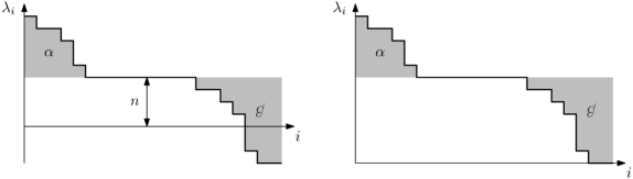
Figure 1: Almost flat highest weights of ${\mathrm{U}}(N)$ (left) and of ${\mathrm{SU}}(N)$ (right).

In this case,

$$c_{2}(\lambda(\alpha,\beta,n))\simeq|\alpha|+|\beta|+n^{2},$$

where we noted $|\alpha|=\sum_{i}\alpha_{i}$. This formula can be interpreted as a sort of decoupling of the partitions $\alpha$, $\beta$ and $(n,\ldots,n)$, and plays a crucial role in the study of the Yang–Mills partition function on compact surfaces.

1.2 Two-dimensional Yang–Mills measure and Wilson loops

The two-dimensional Euclidean Yang–Mills theory is a toy-model for the Yang–Mills theory used in many models of theoretical physics, notably the Standard Model. It was initiated by Migdal [Mig75], then developed mainly by Driver [Dri89], Witten [Wit91], Xu [Xu97], Sengupta [Sen92, Sen97] and Lévy [Lév03]. It can be described as a measure on the connections on a $G$-principal bundle modulo gauge transformations, and it can be reduced to a random matrix model thanks to the holonomy map. Let us briefly describe this construction, borrowed from the approach of Lévy [Lév10]. Consider a compact connected closed surface $\Sigma$ endowed with an area measure $\mathrm{vol}$, a compact group $G$ such that its Lie algebra $\mathfrak{g}$ is endowed with a $G$-invariant inner product, and an oriented topological map on $\Sigma$, that is, an oriented graph $\mathbb{G}=(\mathbb{V},\mathbb{E},\mathbb{E}^{+},\mathbb{F})$ such that all faces of $\mathbb{G}$ are homeomorphic to disks. The Yang–Mills holonomy field is a $G$-valued stochastic process $(H_{\ell})_{\ell\in\mathscr{P}(\mathbb{G})}$ indexed by the set of paths in $\mathbb{G}$ obtained by concatenation of edges and their inverses. The distribution of this process can be described using the configuration space

$$\mathscr{C}_{\mathbb{G}}^{G}=G^{\mathbb{E}^{+}}.$$

The holonomy function is defined for a loop $\ell=e_{1}^{\varepsilon_{1}}\cdots e_{n}^{\varepsilon_{n}}$ as

$$h_{\ell}:\left\{\begin{array}[]{lll}\mathscr{C}_{\mathbb{G}}^{G}&\to&G\\ g&\mapsto&g_{e_{n}}^{\varepsilon_{n}}\cdots g_{e_{1}}^{\varepsilon_{1}},\end{array}\right.$$

and the configuration space is endowed with the smallest sigma-algebra that makes $h_{\ell}$ measurable for any $\ell\in\mathscr{P}(\mathbb{G})$. For any loop $\ell$, the distribution of the random variables $H_{\ell}$ is given by Driver–Sengupta formula

$$\mathbb{E}[f(H_{\ell})]=\frac{1}{Z_{G}(g,T)}\int_{G^{\mathbb{E}^{+}}}f(h_{\ell})\prod_{F\in\mathbb{F}}p_{|F|}(h_{\partial F}(g))\mathrm{d}g,$$ (3)

named after the two mathematicians who derived it initially, Driver on the plane [Dri89], and Sengupta on the sphere [Sen92], then on any compact surface [Sen97]. The quantity $Z_{G}(g,T)$ is a normalisation constant, called partition function, which only depends on the structure group $G$, the genus $g$ of the surface and its total area $T$. Using a kind of Kolmogorov extension theorem, it can be proved that this process is the finite-dimensional marginal of a more general process $(H_{\ell})_{\ell\in\mathscr{P}(\Sigma)}$ indexed by some set of paths $\mathscr{P}(\Sigma)$ on the underlying surface, but we will not need to consider the whole process in this paper: we will only deal with a single simple loop, which can be easily completed into a topological map, and the corresponding holonomy field contains all the informations we want.

We choose to take the unitary group ${\mathrm{U}}(N)$ as the structure group for two main reasons: it is expected to behave nicely when $N$ tends to infinity, since the seminal work of  ’t Hooft [tH74], and it permits to describe the distribution of the Yang–Mills holonomy field in terms of Young diagrams and Schur functions, which have particularly good combinatorial properties. The case of other structure groups can be in fact also treated, and is the result a joint work with A. Dahlqvist [DL22], but does not involve the use of the almost flat highest weights. Instead, we use the fact that the partition functions are bounded and that the Wilson loop expectations on any compact surface of genus $g\geqslant 1$ are absolutely continuous with respect to the Yang–Mills measure on the plane, with density expressed in terms of partition functions.

1.3 Main results

The results of this paper can be divided into two categories: purely algebraic results, which are related to the almost flat highest weights, and probabilistic results related to the expectation and variance of Wilson loops for contractible simple loops on compact surfaces.

In a first part, we study the almost flat highest weights and the corresponding representations. We start by comparing the Casimir numbers of two highest weights whose diagrams are obtained by branching rules: it is Proposition 2.3 in the special unitary case, and Proposition 2.4 in the unitary case. In Proposition 2.5 we estimate, for a highest weight $\lambda_{N}(\alpha,\beta,n)$, the dimension of the corresponding irreducible representation in terms of $\alpha$, $\beta$ and $N$, when $N$ is large.

In a second part, we derive the Wilson loop expectations and variance on a compact connected orientable surface of genus $g\geqslant 1$ in terms of irreducible representations (Proposition 3.3), and apply the results of the first part to obtain their limits (Theorems 3.7 and 3.8. We finally provide a short alternative proof of Theorems 3.7 and 3.8 for a surface of genus $g\geqslant 2$, and this proof only involves constant (flat) highest weights.

2 Almost flat highest weights

The irreducible representations of ${\mathrm{U}}(N)$ are labelled by nonincreasing $N$-tuples of integers $\lambda=(\lambda_{1},\ldots,\lambda_{N})\in{\mathbb{Z}}^{N}$ with $\lambda_{1}\geqslant\cdots\geqslant\lambda_{N}$ (we will use the notation $\lambda=(\lambda_{1}\geqslant\cdots\geqslant\lambda_{N})$ for nonincreasing $N$-tuples) called highest weights, and we denote respectively by $d_{\lambda}$ and $c_{2}(\lambda)$ their dimension and Casimir number, given by

$$d_{\lambda}=\prod_{1\leqslant i<j\leqslant N}\frac{\lambda_{i}-\lambda_{j}+j-i}{j-i}$$ (4)

and

$$c_{2}(\lambda)=\frac{1}{N}\left(\sum_{i=1}^{N}\lambda_{i}^{2}+\sum_{1\leqslant i<j\leqslant N}(\lambda_{i}-\lambda_{j})\right).$$ (5)

The set of irreducible representations is denoted by $\widehat{{\mathrm{U}}}(N)$ and is in bijection with the set of highest weights. The character of a representation of highest weight $\lambda$ is given by the Schur function $s_{\lambda}$, which is a symmetric polynomial when $\lambda_{N}\geqslant 0$ and a symmetric Laurent polynomial otherwise. We will not need its explicit formula for our computations, but refer to [Mac15] and [Sta99] for details about it. The character decomposition (2) of the heat kernel on ${\mathrm{U}}(N)$ becomes then

$$p_{T}(U)=\sum_{\lambda\in\widehat{{\mathrm{U}}}(N)}e^{-c_{2}(\lambda)\frac{T}{2}}d_{\lambda}s_{\lambda}(U),~{}\forall T>0,~{}\forall U\in{\mathrm{U}}(N).$$ (6)

We can make a similar statement for the group ${\mathrm{SU}}(N)$: its irreducible representations are labelled by nonincreasing $N$-tuples of integers $\mu=(\mu_{1}\geqslant\cdots\geqslant\mu_{N}=0)$ also called highest weights, and their dimension and Casimir number are respectively given by

$$d_{\mu}=\prod_{1\leqslant i<j\leqslant N}\frac{\mu_{i}-\mu_{j}+j-i}{j-i}=\prod_{1\leqslant i<j\leqslant N}\left(1+\frac{\mu_{i}-\mu_{j}}{j-i}\right)$$ (7)

and

$$c^{\prime}_{2}(\mu)=\frac{1}{N}\left(\sum_{i=1}^{N}\mu_{i}^{2}-\frac{1}{N}\left(\sum_{i=1}^{N}\mu_{i}\right)^{2}+\sum_{1\leqslant i<j\leqslant N}(\mu_{i}-\mu_{j})\right).$$ (8)

The Equation (6) still holds for ${\mathrm{SU}}(N)$ when one replaces accordingly the highest weights and their related quantities $d_{\lambda}$ and $c_{2}(\lambda)$.

2.1 Partition decomposition of highest weights

From two integer partitions $\alpha=(\alpha_{1}\geqslant\cdots\geqslant\alpha_{r}>0)$ and $\beta=(\beta_{1}\geqslant\cdots\geqslant\beta_{s}>0)$ of respective lengths $\ell(\alpha)=r$ and $\ell(\beta)=s$, and an integer $n\in{\mathbb{Z}}$, we can form, for all $N\geqslant r+s+1$, the composite highest weight

$$\lambda_{N}(\alpha,\beta,n)=(\alpha_{1}+n,\ldots,\alpha_{r}+n,\underbrace{n,\ldots,n}_{N-r-s},n-\beta_{s},\ldots,n-\beta_{1})\in\widehat{\mathrm{U}}(N).$$ (9)

We extend this definition in the obvious way to the cases where one or both of the partitions $\alpha$ and $\beta$ are the empty partition.

We can also form the highest weight

$$\lambda_{N}(\alpha,\beta)=\lambda_{N}(\alpha,\beta,\beta_{1})\in\widehat{\mathrm{SU}}(N),$$

with the convention that $\lambda_{N}(\alpha,\varnothing)=\lambda_{N}(\alpha,\varnothing,0)=(\alpha_{1},\ldots,\alpha_{r},0)$.

There is a natural bijection $\Phi:\widehat{{\mathrm{SU}}}(N)\times{\mathbb{Z}}\simeq\widehat{{\mathrm{U}}}(N)$ that “shifts” the highest weights of ${\mathrm{SU}}(N)$ into highest weights of ${\mathrm{U}}(N)$, and that is given by

$$\Phi(\lambda,n)=(\lambda_{1}+n,\ldots,\lambda_{N}+n),\ \forall\lambda\in\widehat{{\mathrm{SU}}}(N),\ \forall n\in{\mathbb{Z}}.$$ (10)

We will write $\lambda+n=\Phi(\lambda,n)$ to simplify the notations; it is easy to check that, given two partitions $\alpha$ and $\beta$ and any integer $n\in{\mathbb{Z}}$:

$$\lambda_{N}(\alpha,\beta,n)=\lambda_{N}(\alpha,\beta)+n-\beta_{1}.$$

Most of the results we will present are actually easier to prove for highest weights of ${\mathrm{SU}}(N)$, and they will be extended to ${\mathrm{U}}(N)$ using the bijection $\Phi$.

We proved in [Lem21] that these constructions can be reversed, in the sense that given a highest weight $\lambda\in\widehat{{\mathrm{U}}}(N)$, then we can define unambiguously $\alpha,\beta$ and $n$ such that $\lambda=\lambda_{N}(\alpha,\beta,n)$. In this case, we will denote them by $\alpha_{\lambda},\beta_{\lambda}$ and $n_{\lambda}$ to emphasize the fact that they are determined by $\lambda$. However, it does not necessarily mean that one can express the irreducible representations with highest weight $\lambda$ using $\alpha$, $\beta$ and $n$. In fact, the weights of interest will be $\lambda_{N}(\alpha,\beta,n)$ such that $\alpha$ and $\beta$ are small perturbations of the constant weight $(n,\ldots,n)$. Such weights were already studied by Gross and Taylor in [GT93] for finite $\alpha$ and $\beta$. Our approach actually enables $\alpha$ and $\beta$ to grow with $N$ while remaining small enough, so that $\lambda_{N}(\alpha,\beta,n)$ remains close to $(n,\ldots,n)$, i.e., “almost flat”.

2.2 Casimir number

In this section, we will prove several estimations of the Casimir numbers of ${\mathrm{SU}}(N)$ and ${\mathrm{U}}(N)$. Recall that the content of the box $(i,j)$ of a diagram corresponding to the partition $\alpha=(\alpha_{1}\geqslant\cdots\geqslant\alpha_{r}>0)$ is the quantity $c(i,j)=j-i$, and that the total content $K(\alpha)$ of the diagram is the sum of contents of all its boxes. We denote also by $|\alpha|$ the sum of the parts of the partition: $|\alpha|=\alpha_{1}+\cdots+\alpha_{r}$. The Casimir numbers of composite highest weights are described by the following proposition proved in [Lem21].

Proposition 2.1.

Let $\alpha$ and $\beta$ be two partitions of respective lengths $r$ and $s$. Let $n$ be an integer. Then, provided $N\geqslant r+s$, we have

$$c_{2}(\lambda(\alpha,\beta,n))=|\alpha|+|\beta|+n^{2}+\frac{2}{N}\big{(}K(\alpha)+K(\beta)+n(|\alpha|-|\beta|)\big{)}$$ (11)

in the unitary case, and

$$c^{\prime}_{2}(\lambda(\alpha,\beta))=|\alpha|+|\beta|+\frac{2}{N}(K(\alpha)+K(\beta))-\frac{1}{N^{2}}\left(|\alpha|-|\beta|\right)^{2}$$ (12)

in the special unitary case.

A direct consequence of this proposition is given by this fundamental estimation.

Lemma 2.2.

Let $\lambda\in\widehat{{\mathrm{SU}}}(N)$. Set $k=|\alpha_{\lambda}|+|\beta_{\lambda}|$. Then the following inequalities hold:

$$k-\frac{k^{2}}{N}-\frac{k^{2}}{N^{2}}\leqslant c^{\prime}_{2}(\lambda)\leqslant k+\frac{k^{2}}{N},$$ (13)

$$\frac{k}{2}\leqslant c^{\prime}_{2}(\lambda).$$ (14)

Proof.

We start from the expression of $c^{\prime}_{2}(\lambda(\alpha,\beta))$ given by (12). The point is to bound $K(\alpha)$ and $K(\beta)$.

The list of the contents of the boxes of $\alpha$ taken row after row and from left to right in each row is a sequence $x_{1},\ldots,x_{|\alpha|}$ such that $|x_{i}|\leqslant i-1$ for each $i\in\{1,\ldots,|\alpha|\}$. It follows that

$$-|\alpha|(|\alpha|-1)\leqslant 2K(\alpha)\leqslant|\alpha|(|\alpha|-1).$$

This implies immediately

$$2|K(\alpha)+K(\beta)|\leqslant k^{2},$$

and (13), after observing that $0\leqslant(|\alpha|-|\beta|)^{2}\leqslant(|\alpha|+|\beta|)^{2}=k^{2}$.

Let us turn to the proof of (14). Using (12) and the fact that the content of a diagram $\alpha=(\alpha_{1},\ldots,\alpha_{r})$ satisfies

$$2K(\alpha)=\sum_{i}\alpha_{i}^{2}+\sum_{i<j}(\alpha_{i}-\alpha_{j})-r|\alpha|,$$

we obtain

$$Nc^{\prime}_{2}(\lambda(\alpha,\beta))= (N-r)|\alpha|+(N-s)|\beta|+\left[\sum_{i=1}^{r}\alpha_{i}^{2}-\frac{1}{N}|\alpha|^{2}\right]+\left[\sum_{i=1}^{s}\beta_{i}^{2}-\frac{1}{N}|\beta|^{2}\right]$$

$$+\left[\sum_{1\leqslant i<j\leqslant r}(\alpha_{i}-\alpha_{j})\right]+\left[\sum_{1\leqslant i<j\leqslant s}(\beta_{i}-\beta_{j})\right]+\left[\frac{2}{N}|\alpha||\beta|\right].$$

It is clear that every term in square brackets is nonnegative, which implies

$$c^{\prime}_{2}(\lambda(\alpha,\beta))\geqslant\left(|\alpha|+|\beta|\right)\left(1-\frac{\min(r,s)}{N}\right)\geqslant\frac{k}{2},$$

as expected. ∎

The first inequality of Lemma 2.2 states that, provided that $|\alpha|+|\beta|$ is small enough:

$$c^{\prime}_{2}(\lambda_{N}(\alpha,\beta))\simeq|\alpha|+|\beta|.$$

The second one provides a lower bound of the Casimir number for any highest weight. Before giving other estimations, we need to introduce two notations: if $\lambda$ and $\mu$ are two highest weights, both of ${\mathrm{U}}(N)$ or both of ${\mathrm{SU}}(N)$, we will write $\mu\nearrow\lambda$ (or $\lambda\searrow\mu$) if $\lambda$ can be obtained from $\mu$ by adding $1$ to one of its parts, and $\mu\sim\lambda$ if $\lambda$ can be obtained from $\mu$ by adding $1$ to one of its parts and $-1$ to one of its parts, i.e. if there exists a highest weight $\nu$ such that $\lambda\nearrow\nu$ and $\mu\nearrow\nu$. These branching rules are illustrated in Fig. 2.

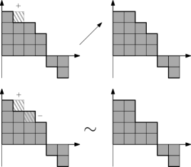
Figure 2: On the first row: we have $\lambda\nearrow\mu$, with the diagram of $\lambda$ on the left and the one of $\mu$ on the right. On the second row: we have $\lambda\sim\mu$, with the diagram of $\lambda$ on the left and the one of $\mu$ on the right.

Proposition 2.3.

Let $(\lambda,\mu)\in\widehat{{\mathrm{SU}}}(N)^{2}$ be two highest weights and set $\alpha=\alpha_{\mu}$ and $\beta=\beta_{\mu}$. If $\lambda\searrow\mu$ or if $\lambda\sim\mu$, then we have for $N$ large enough

$$-\frac{T}{2}c^{\prime}_{2}(\mu)+\frac{t}{2}(c^{\prime}_{2}(\mu)-c^{\prime}_{2}(\lambda))\leqslant-\frac{T}{8}(|\alpha|+|\beta|)+t.$$ (15)

Proof.

Let us start with The case when $\lambda\searrow\mu$. Let $i_{0}$ be the index such that $\lambda_{i_{0}}=\mu_{i_{0}}+1$. From the definitions of $c^{\prime}_{2}(\mu)$ and $c^{\prime}_{2}(\lambda)$ (see (8)) and the fact that $i_{0}\leqslant N$, we have the estimation

$$c^{\prime}_{2}(\lambda)-c^{\prime}_{2}(\mu)=1+\frac{2(\mu_{i_{0}}+1-i_{0})}{N}-\frac{2|\mu|+1}{N^{2}}\geqslant-2-\frac{2|\mu|}{N^{2}}.$$

From (14) and the fact that $|\mu|=|\alpha|-|\beta|+N\beta_{1}\leqslant|\alpha|+N|\beta|$, we then get

$$-\frac{T}{2}c^{\prime}_{2}(\mu)+\frac{t}{2}(c^{\prime}_{2}(\mu)-c^{\prime}_{2}(\lambda))\leqslant -\frac{T}{4}(|\alpha|+|\beta|)+\frac{t}{2N^{2}}(|\alpha|+N|\beta|)+t$$

$$\leqslant (|\alpha|+|\beta|)\left(\frac{t}{2N}-\frac{T}{4}\right)+t,$$

and the inequality (15) is satisfied for $N$ such that $\frac{t}{2N}<\frac{T}{8}$.

Now let us prove the case when $\lambda\sim\mu$. If $\lambda=\mu$ then the result directly follows from Lemma 2.2. Otherwise, there are $i_{0}\neq j_{0}$ such that $\lambda_{i_{0}}=\mu_{i_{0}}+1$, $\lambda_{j_{0}}=\mu_{j_{0}}-1$ and $\lambda_{i}=\mu_{i},\ \forall i\not\in\{i_{0},j_{0}\}$. Using the definition of Casimir number, we have

$$c^{\prime}_{2}(\mu)-c^{\prime}_{2}(\lambda)=\frac{2(\mu_{j_{0}}-\mu_{i_{0}}+i_{0}-j_{0}-1)}{N}.$$

As $\mu_{1}\geqslant\cdots\geqslant\mu_{N}$, we have $\mu_{1}-1>\cdots>\mu_{N}-N$ and in particular

$$0<\mu_{i}-\mu_{j}+j-i\leqslant\mu_{1}+N-1,\ \forall i<j.$$

If $i_{0}<j_{0}$ then we have $c^{\prime}_{2}(\mu)-c^{\prime}_{2}(\lambda)\leqslant 0$ and the bound given by the case $\lambda=\mu$ still holds. Otherwise, we have

$$c^{\prime}_{2}(\mu)-c^{\prime}_{2}(\lambda)\leqslant\frac{2(\mu_{1}+N-2)}{N}\leqslant 2+\frac{2\mu_{1}}{N}.$$

Since $\mu_{1}=\alpha_{1}+\beta_{1}\leqslant|\alpha|+|\beta|$ and using Lemma 2.2 we obtain

$$-\frac{T}{2}c^{\prime}_{2}(\mu)+\frac{t}{2}(c^{\prime}_{2}(\mu)-c^{\prime}_{2}(\lambda))\leqslant (|\alpha|+|\beta|)\left(\frac{t}{N}-\frac{T}{4}\right)+t.$$

The inequality follows, when $N$ satisfies $\frac{t}{N}<\frac{T}{8}$. ∎

We can also mention a similar result, that will be used to prove Theorem 3.7 in the unitary case, and which is a direct consequence of Proposition 2.1.

Proposition 2.4.

Let $\alpha=(\alpha_{1}\geqslant\cdots\geqslant\alpha_{r})$ and $\beta=(\beta_{1}\geqslant\cdots\geqslant\beta_{s})$ be integer partitions, $(n,N)\in{\mathbb{Z}}^{2}$ be two integers, such that $N\geqslant r+s+1$.

1. If $\alpha^{\prime}$ is a partition such that $\alpha^{\prime}\searrow\alpha$ and $i_{0}$ is the index such that $\alpha^{\prime}_{i_{0}}=\alpha_{i_{0}}+1$, then

   $$c_{2}(\lambda_{N}(\alpha,\beta,n))-c_{2}(\lambda_{N}(\alpha^{\prime},\beta,n))=-1-\frac{2}{N}(\alpha_{i_{0}}+n+1-i_{0}).$$ (16)

2. If $\beta^{\prime}$ is a partition such that $\beta^{\prime}\nearrow\beta$ and $i_{0}$ is the index such that $\beta_{i_{0}}=\beta^{\prime}_{i_{0}}+1$, then

   $$c_{2}(\lambda_{N}(\alpha,\beta,n))-c_{2}(\lambda_{N}(\alpha,\beta^{\prime},n))=1+\frac{2}{N}(\beta_{i_{0}}-n-i_{0}).$$ (17)

From now on, let us fix a real $\gamma\in(0,\frac{1}{3})$, that we can consider as a control parameter. We split the set of highest weights of ${\mathrm{SU}}(N)$ in four disjoint subsets:

$$\begin{split}\Lambda_{N,1}^{\gamma}&=\{\lambda\in\widehat{{\mathrm{SU}}}(N):|\alpha_{\lambda}|\leqslant N^{\gamma},|\beta_{\lambda}|\leqslant N^{\gamma}\},\\ \Lambda_{N,2}^{\gamma}&=\{\lambda\in\widehat{{\mathrm{SU}}}(N):|\alpha_{\lambda}|>N^{\gamma},|\beta_{\lambda}|\leqslant N^{\gamma}\},\\ \Lambda_{N,3}^{\gamma}&=\{\lambda\in\widehat{{\mathrm{SU}}}(N):|\alpha_{\lambda}|\leqslant N^{\gamma},|\beta_{\lambda}|>N^{\gamma}\},\\ \Lambda_{N,4}^{\gamma}&=\{\lambda\in\widehat{{\mathrm{SU}}}(N):|\alpha_{\lambda}|>N^{\gamma},|\beta_{\lambda}|>N^{\gamma}\}.\end{split}$$ (18)

We can do the same for highest weights of ${\mathrm{U}}(N)$, but the subsets will be denoted by $\Omega_{N,i}^{\gamma}$ instead of $\Lambda_{N,i}^{\gamma}$. In this framework, (13) can be refined as the following for any highest weight $\lambda\in\Lambda_{N,1}^{\gamma}$, called almost flat:

$$|\alpha_{\lambda}|+|\beta_{\lambda}|-4N^{2\gamma-1}-4N^{2\gamma-2}\leqslant c^{\prime}_{2}(\lambda)\leqslant|\alpha_{\lambda}|+|\beta_{\lambda}|+4N^{2\gamma-1}.$$ (19)

We can rewrite this as

$$\left|c^{\prime}_{2}(\lambda)-\big{(}|\alpha_{\lambda}|+|\beta_{\lambda}|\big{)}\right|\leqslant 8N^{2\gamma-1}.$$ (20)

Another crucial point is the following: for $N$ large enough, any partition of an integer not greater than $N^{\gamma}$ has less than $\frac{N}{2}$ positive parts. Thus, if $\alpha$ and $\beta$ are any two such partitions, the highest weight $\lambda_{N}(\alpha,\beta)$ is well defined, and belongs to $\Lambda_{N,1}^{\gamma}$. As a consequence, for $N$ large enough,

$$\Lambda_{N,1}^{\gamma}=\{\lambda_{N}(\alpha,\beta),\alpha\vdash r,\beta\vdash s:r\leqslant N^{\gamma},s\leqslant N^{\gamma}\}.$$ (21)

Using the bijection $\Phi$ given in (10), we get as well for almost flat highest weights of ${\mathrm{U}}(N)$ with $N$ large enough,

$$\Omega_{N,1}^{\gamma}=\{\lambda_{N}(\alpha,\beta,n),\alpha\vdash r,\beta\vdash s:r\leqslant N^{\gamma},s\leqslant N^{\gamma},n\in{\mathbb{Z}}\}.$$ (22)

2.3 Dimension

The dimension of almost flat highest weights can also be related to the dimension of irreducible representations of the symmetric group.

Proposition 2.5.

Let $\alpha=(\alpha_{1}\geqslant\cdots\geqslant\alpha_{r})$ and $\beta=(\beta_{1}\geqslant\cdots\geqslant\beta_{s})$ be two integer partitions, $N\geqslant r+s+1$ an integer and $\gamma\in(0,\tfrac{1}{3})$ a real number. Let us assume that $|\alpha|\leqslant N^{\gamma}$ and $|\beta|\leqslant N^{\gamma}$. The partitions $\alpha$ and $\beta$ induce two highest weights of ${\mathrm{SU}}(N)$, $\tilde{\alpha}=\lambda_{N}(\alpha,\varnothing)$ and $\tilde{\beta}=\lambda_{N}(\beta,\varnothing)$. We have the following facts.

1. If we set $d^{\alpha}$ as the dimension of the irreducible representation of $\mathfrak{S}_{|\alpha|}$ associated with $\alpha$, then, assuming that $N$ is large enough,

   $$\frac{d^{\alpha}N^{|\alpha|}}{|\alpha|!}(1-2N^{2\gamma-1})\leqslant d_{\tilde{\alpha}}\leqslant\frac{d^{\alpha}N^{|\alpha|}}{|\alpha|!}(1+2N^{2\gamma-1}),$$ (23)

   and the same result holds for $\beta$.

2. For any $n\in{\mathbb{Z}}$, the dimension of $\lambda_{N}(\alpha,\beta,n)$ satisfies the following estimation, assuming that $N$ is large enough:

   $$\frac{d^{\alpha}d^{\beta}N^{|\alpha|+|\beta|}}{|\alpha|!|\beta|!}(1-24N^{3\gamma-1})\leqslant d_{\lambda_{N}(\alpha,\beta,n)}\leqslant\frac{d^{\alpha}d^{\beta}N^{|\alpha|+|\beta|}}{|\alpha|!|\beta|!}(1+24N^{3\gamma-1})$$ (24)

Note that this proposition generalizes a result by Gross and Taylor: in [GT93], they derived similar asymptotic expansions but in the case where $|\alpha|$ and $|\beta|$ were finite and not depending on $N$. However, we really need the stronger assumption $|\alpha|,|\beta|\leqslant N^{\gamma}$ as we will see later.

Proof of Proposition 2.5.

$(i)$ let us first recall that (cf. [GT93, VO04])

$$d_{\tilde{\alpha}}=\frac{d^{\alpha}N^{|\alpha|}}{|\alpha|!}\prod_{\begin{subarray}{c}1\leqslant i\leqslant r\\ 1\leqslant j\leqslant\alpha_{i}\end{subarray}}\left(1+\frac{j-i}{N}\right).$$ (25)

But for any $1\leqslant i\leqslant r$ and $1\leqslant j\leqslant\alpha_{i}$, we have $1-r\leqslant j-i\leqslant\alpha_{i}-1$, and under the assumption $|\alpha|\leqslant N^{\gamma}$ it implies that $|j-i|\leqslant N^{\gamma}$. Thus,

$$(1-N^{\gamma-1})^{|\alpha|}\leqslant\prod_{\begin{subarray}{c}1\leqslant i\leqslant r\\ 1\leqslant j\leqslant\alpha_{i}\end{subarray}}\left(1+\frac{j-i}{N}\right)\leqslant(1+N^{\gamma-1})^{|\alpha|}.$$

From the convexity inequality of the exponential function, we have

$$(1+N^{\gamma-1})^{|\alpha|}\leqslant e^{|\alpha|N^{\gamma-1}}.$$

We can use the following reverse inequalities, that hold for any $x\in(0,\tfrac{1}{2})$:

$$e^{x}\leqslant 1+2x,\ \log(1-x)\geqslant-2x.$$

It implies that, for $N$ such that $N^{\gamma-1}<\tfrac{1}{2}$ (which is true for $N$ large enough),

$$1-2N^{2\gamma-1}\leqslant e^{-2|\alpha|N^{\gamma-1}}\leqslant(1-N^{\gamma-1})^{|\alpha|}\leqslant\prod_{\begin{subarray}{c}1\leqslant i\leqslant r\\ 1\leqslant j\leqslant\alpha_{i}\end{subarray}}\left(1+\frac{j-i}{N}\right)\leqslant e^{|\alpha|N^{\gamma-1}}\leqslant 1+2N^{2\gamma-1}.$$

This estimation, applied to (25), gives the expected result.

$(ii)$ Let us first remark that, from the Weyl dimension formula, we have for any $n\in{\mathbb{Z}}$

$$d_{\lambda_{N}(\alpha,\beta,n)}=d_{\tilde{\alpha}}d_{\tilde{\beta}}Q(\alpha,\beta),$$ (26)

with

$$Q(\alpha,\beta)=\prod_{\begin{subarray}{c}1\leqslant i\leqslant r\\ 1\leqslant j\leqslant s\end{subarray}}\frac{(N+1-i-j)(\alpha_{i}+\beta_{j}+N+1-i-j)}{(\alpha_{i}+N+1-i-j)(\beta_{j}+N+1-i-j)}.$$

As $r\leqslant|\alpha|$ and $s\leqslant|\beta|$, the assumption $|\alpha|,|\beta|\leqslant N^{\gamma}$ implies that we also have $r,s\leqslant N^{\gamma}$. For any $1\leqslant i\leqslant r$ and $1\leqslant j\leqslant s$, we have therefore

$$-2N^{\gamma}\leqslant 3-2N^{\gamma}\leqslant\alpha_{i}+\beta_{j}-i-j+1\leqslant 2N^{\gamma}-1\leqslant 2N^{\gamma}.$$

It implies that

$$\left|\frac{1+\alpha_{i}+\beta_{j}-i-j}{N}\right|\leqslant 2N^{\gamma-1},$$

and we have the same bound for $\left|\frac{1+\alpha_{i}-i-j}{N}\right|$, $\left|\frac{1+\beta_{j}-i-j}{N}\right|$ and $\left|\frac{1-i-j}{N}\right|$, so that

$$Q(\alpha,\beta)=\prod_{\begin{subarray}{c}1\leqslant i\leqslant r\\ 1\leqslant j\leqslant s\end{subarray}}\frac{(1+A_{N}(i,j))(1+B_{N}(i,j))}{(1+C_{N}(i,j))(1+D_{N}(i,j))},$$

with $|A_{N}(i,j)|,|B_{N}(i,j)|,|C_{N}(i,j)|,|D_{N}(i,j)|\leqslant 2N^{\gamma-1}$.

For any $(i,j)$ we have

$$\frac{1}{C_{N}(i,j)}=1-\frac{1+C_{N}(i,j)}{1+C_{N}(i,j)}=1+C^{\prime}_{N}(i,j),$$

with $|C^{\prime}_{N}(i,j)|\leqslant 2|C_{N}(i,j)|$, and the same result holds for $D_{N}(i,j)$. It implies that

$$Q(\alpha,\beta)=\prod_{\begin{subarray}{c}1\leqslant i\leqslant r\\ 1\leqslant j\leqslant s\end{subarray}}(1+A_{N}(i,j))(1+B_{N}(i,j))(1+C^{\prime}_{N}(i,j))(1+D^{\prime}_{N}(i,j)),$$

with $|A_{N}(i,j)|,|B_{N}(i,j)|,|C^{\prime}_{N}(i,j)|,|D^{\prime}_{N}(i,j)|\leqslant 4N^{\gamma-1}$. Hence, using the same inequalities as in $(i)$ we get the estimation

$$e^{-8N^{3\gamma-1}}\leqslant(1-4N^{\gamma-1})^{N^{2\gamma}}\leqslant Q(\alpha,\beta)\leqslant(1+4N^{\gamma-1})^{N^{2\gamma}}\leqslant e^{4N^{3\gamma-1}},$$

which implies

$$1-8N^{3\gamma-1}\leqslant Q(\alpha,\beta)\leqslant 1+8N^{3\gamma-1}.$$

We can apply this, as well as the point $(i)$, to get for $N^{2\gamma-1}<\tfrac{1}{4}$ (which is in particular true for $N$ large enough)

$$d_{\lambda_{N}(\alpha,\beta,n)}\leqslant\frac{d^{\alpha}d^{\beta}N^{|\alpha|+|\beta|}}{|\alpha|!|\beta|!}(1+2N^{2\gamma-1})^{2}(1+8N^{3\gamma-1}),$$

which can be simplified considering that for $(x,y,z)\in(0,\tfrac{1}{4})^{3}$ such that $x+y+z<\tfrac{1}{4}$,

$$(1+x)(1+y)(1+z)\leqslant e^{x+y+z}\leqslant 1+2(x+y+z).$$

Indeed, for $N$ such that $N^{3\gamma-1}+2N^{2\gamma-1}<\tfrac{1}{4}$ we obtain

$$d_{\lambda_{N}(\alpha,\beta,n)}\leqslant\frac{d^{\alpha}d^{\beta}N^{|\alpha|+|\beta|}}{|\alpha|!|\beta|!}(1+8N^{2\gamma-1}+16N^{3\gamma-1})\leqslant\frac{d^{\alpha}d^{\beta}N^{|\alpha|+|\beta|}}{|\alpha|!|\beta|!}(1+24N^{3\gamma-1}),$$

and

$$d_{\lambda_{N}(\alpha,\beta,n)}\geqslant\frac{d^{\alpha}d^{\beta}N^{|\alpha|+|\beta|}}{|\alpha|!|\beta|!}(1-24N^{3\gamma-1}),$$

which proves the result. ∎

There exists a more general formula, due to Koike [Koi89], that decomposes $s_{\lambda(\alpha,\beta,0)}$ in terms of Schur functions of sub-diagrams, using Littlewood–Richardson coefficients $(c_{\lambda,\mu}^{\nu})$.

Theorem 2.6.

Let $\alpha\vdash k$, $\beta\vdash\ell$, and $n\geqslant\ell(\alpha)+\ell(\beta)$, then

$$s_{\lambda(\alpha,\beta,0)}(x)=\sum_{\begin{subarray}{c}p_{1},p_{2},p_{3}\geqslant 0\\ p_{1}+p_{2}=k,p_{1}+p_{3}=\ell\end{subarray}}\sum_{\begin{subarray}{c}\mu\vdash p_{1},\alpha_{1}\vdash p_{2},\beta_{1}\vdash p_{3}\\ \alpha_{1}\subset\alpha,\beta_{1}\subset\beta\end{subarray}}c_{\mu,\alpha_{1}}^{\alpha}c_{\mu^{\prime},\beta_{1}}^{\beta}s_{\alpha_{1}}(x)s_{\beta_{1}}(x^{-1}),\ \forall x\in{\mathrm{U}}(N),$$ (27)

where $\mu^{\prime}$ is the transposed diagram of $\mu$.

It is not clear whether one could recover Equation (24) from (27), or if this decomposition fits the regime of almost flat highest weights. Though it provides an exact decomposition, the latter involves a large number of diagrams and Littlewood–Richardson coefficients, which makes asymptotic estimations truly challenging. However, Magee [Mag22] was able to get an asymptotic estimation of $d_{\lambda(\alpha,\beta,0)}$ for fixed $\alpha$ and $\beta$ using Theorem 2.6.

Corollary 2.7.

Let $\alpha\vdash k$ and $\beta\vdash\ell$. For $N\geqslant\ell(\alpha)+\ell(\beta)$, $d_{\lambda_{N}(\alpha,\beta,0)}$ is given by a polynomial function of $N$ with coefficients in $\mathbb{Q}$ and

$$d_{\lambda_{N}(\alpha,\beta,0)}\asymp N^{k+\ell}.$$

3 Wilson loop expectations for simple loops

In this section, we discuss the convergence of Wilson loops for contractible simple loops on a surface. We first recall the cases of the plane and the sphere, which have been proved earlier, then we will state the results for compact surfaces of higher genus.

3.1 The plane and the sphere

Figure 3: A simple loop enclosing a domain of area $t$, embedded in the plane (on the left) or in the sphere $\mathbb{S}^{2}$ (on the right).

The first building brick of the master field is the Wilson loop functional for a loop with no self-intersection, which we will call a simple loop. If it is embedded in the plane, it is the boundary of a domain with area $t$, and if it is embedded in the sphere it separates it into two domains of respective areas $t$ and $T-t$, as illustrated in Fig. 3. If we complete this into an admissible graph, it enables us to apply Driver–Sengupta formula (3) in order to compute the Wilson loop expectation $W_{\ell}=\mathbb{E}[\mathrm{tr}(H_{\ell})]$. Recall that we denote by $(p_{t})_{t\geqslant 0}$ the heat kernel on the structure group $G$.

Proposition 3.1.

Let $\Sigma$ be either the plane $\mathbb{R}^{2}$ or the sphere $\mathbb{S}^{2}$ with area $T$, $\ell$ be a simple loop on $\Sigma$, oriented counterclockwise. The Wilson loop expectation $W_{\ell}$ is equal to

$$W_{\ell}= \int_{G}\mathrm{tr}(x)p_{t}(x)\mathrm{d}x, \text{if }\Sigma\text{ is the plane},$$ (28)

$$W_{\ell}= \frac{1}{Z_{T}}\int_{G}\mathrm{tr}(x)p_{t}(x)p_{T-t}(x^{-1})\mathrm{d}x, \text{if }\Sigma\text{ is the sphere}.$$ (29)

In (29), the density $p_{t}(x)p_{T-t}(x^{-1})/Z_{T}$ is nothing but the density at time $t$ of a Brownian bridge $(B_{t})_{t\in[0,T]}$ on $G$ such that $B_{0}=B_{T}=e$. It follows from the convolution property of the heat semigroup that $Z_{T}=\int_{G}p_{t}(x)p_{T-t}(x^{-1})\mathrm{d}x=p_{T}(e)$.

There are various ways of computing Wilson loop expectations, which are closely related to the computation of moments of the Brownian motion (or Brownian bridge, depending wether the underlying surface is the plane or the sphere) on ${\mathrm{U}}(N)$. We will present one of them, that we will be using later: (noncommutative) harmonic analysis on ${\mathrm{U}}(N)$. Among the various tool that can be used, let us list a few ones:

• Matrix stochastic calculus, which is treated in [Gui04];

• Schur–Weyl duality, which is used in [Lév08, CDK18] to compute the limit of moments of unitary Brownian motion;

• Free stochastic calculus, which is used in [BS01] to compute the limit of matrix integrals similar to the Wilson loops expectations (but with respect to Hermitian Brownian motion instead of the unitary one);

• Determinantal point processes, which are used in [LW16] to compute the asymptotic distribution of a unitary Brownian bridge;

• Large deviations, which are depicted in [Gui04] and used in [LM15] to compute the same limit as in [LW16].

The use of noncommutative harmonic analysis in order to compute integrals such as (28) or (29) is based to the heat kernel decomposition (2). For $G={\mathrm{U}}(N)$, Eq. (28) becomes

$$W_{\ell}=\sum_{\lambda\in\widehat{{\mathrm{U}}}(N)}e^{-c_{2}(\lambda)\frac{t}{2}}d_{\lambda}\int_{{\mathrm{U}}(N)}\mathrm{tr}(x)s_{\lambda}(x)\mathrm{d}x,$$ (30)

and (29) becomes

$$W_{\ell}=\frac{1}{Z_{T}}\sum_{\lambda,\mu\in\widehat{{\mathrm{U}}}(N)}e^{-c_{2}(\lambda)\frac{t}{2}-c_{2}(\mu)\frac{T-t}{2}}d_{\lambda}d_{\mu}\int_{{\mathrm{U}}(N)}\mathrm{tr}(x)s_{\lambda}(x)s_{\mu}(s^{-1})\mathrm{d}x.$$ (31)

We can notice that in both equations the integrals do not depend anymore on $t$ or $T$. In order to compute them, we must be able to evaluate the product $\mathrm{tr}(\cdot)s_{\lambda}(\cdot)$. As it is a bounded (hence square integrable) central function, it decomposes on the Hilbert basis of irreducible characters, and the coefficients are given by the Murnaghan–Nakayama rule, which is given below. We will use the following notation: $\lambda\prec\mu$ or $\mu\succ\lambda$ when $\lambda\subset\mu$ and $\mu-\lambda$ is a border strip, i.e. it is connected and contains no $2\times 2$ block of squares. The height of a border strip is defined as

$$\mathrm{ht}(\mu-\lambda)=\#\{i:\mu_{i}-\lambda_{i}\neq 0\}-1,$$

and its length $|\mu-\lambda|$ is simply the number of boxes it contains, and is equal to

$$|\mu-\lambda|=|\mu|-|\lambda|.$$

We note $\lambda\prec_{n}\mu$ (resp. $\mu\succ_{n}\lambda$) if $\lambda\prec\mu$ (resp. $\mu\succ\lambda$) and $|\mu-\lambda|=n$, for $n\in{\mathbb{N}}$. In particular, $\lambda\prec_{1}\mu$ if and only if $\lambda\nearrow\mu$. We can now state the Murnaghan–Nakayama rule, whose proof can be found in [Mac15, I.7, example 5] .

Lemma 3.2 (Murnaghan–Nakayama rule).

Let $\lambda\in\widehat{{\mathrm{U}}}(N)$ be a highest weight, $r$ a positive integer. Then we have

$$\mathrm{Tr}(x^{r})s_{\lambda}(x)=\sum_{\begin{subarray}{c}\mu\in\widehat{{\mathrm{U}}}(N)\\ \mu\succ_{r}\lambda\end{subarray}}(-1)^{\mathrm{ht}(\mu-\lambda)}s_{\mu}(x),\ \forall x\in{\mathrm{SU}}(N).$$ (32)

In particular, for $r=1$, we have

$$\mathrm{Tr}(x)s_{\lambda}(x)=\sum_{\begin{subarray}{c}\mu\in\widehat{{\mathrm{U}}}(N)\\ \mu\searrow\lambda\end{subarray}}s_{\mu}(x),\ \forall x\in{\mathrm{U}}(N).$$ (33)

Using (33), we have in the plane

$$W_{\ell}=\frac{1}{N}\sum_{\lambda\in\widehat{{\mathrm{U}}}(N)}e^{-c_{2}(\lambda)\frac{t}{2}}d_{\lambda}\sum_{\begin{subarray}{c}\mu\in\widehat{{\mathrm{U}}}(N)\\ \mu\searrow\lambda\end{subarray}}\int_{{\mathrm{U}}(N)}s_{\mu}(x)\mathrm{d}x.$$ (34)

As the integral $\int_{{\mathrm{U}}(N)}s_{\mu}(x)\mathrm{d}x$ is equal to $1$ if $\mu=(0,\ldots,0)$ and $0$ otherwise, it appears that

$$W_{\ell}=e^{-c_{2}((0,\ldots,0,-1))\frac{t}{2}}d_{(0,\ldots,0,-1)}.$$ (35)

A direct computation of the Casimir number and the dimension of the representation yields

$$W_{\ell}=e^{-\frac{t}{2}},$$ (36)

which trivially converges to $e^{-\tfrac{t}{2}}$ when $N\to\infty$.

In the case of the sphere, with similar arguments we obtain

$$W_{\ell}=\frac{1}{NZ_{T}}\sum_{\begin{subarray}{c}\lambda,\mu\in\widehat{{\mathrm{U}}}(N)\\ \lambda\nearrow\mu\end{subarray}}e^{-c_{2}(\lambda)\frac{t}{2}-c_{2}(\mu)\frac{T-t}{2}}d_{\lambda}d_{\mu}.$$ (37)

It is much more complicated to compute the limit of such a quantity, because it is a sum over a set of indices whose size depends on $N$, and thus it cannot be treated as a simple series. Dahlqvist and Norris [DN20] found a way to pass through this obstacle, using the empirical distribution of the highest weights

$$\mu_{\lambda}=\frac{1}{N}\sum_{i=1}^{N}\delta_{\lambda_{i}},\ \forall\lambda\in\widehat{{\mathrm{U}}}(N).$$

Indeed, they applied a large deviation principle found by Guionnet and Maïda in [GM05], and they used some concentration results as well as contour integrals making rigorous the arguments already present in [Bou94], to show that

$$\lim_{N\to\infty}W_{\ell}=\frac{2}{n\pi}\int_{0}^{\infty}\cosh((2t-T)\tfrac{x}{2})\sin(\pi\rho_{T}(x))\mathrm{d}x.$$ (38)

In the equation above, $\rho_{T}$ denotes the density, with respect to Lebesgue measure, of the minimizer of the functional $\mathscr{I}_{T}$ on the set $\mathcal{M}_{1}(\mathbb{R})$ of probability measures on $\mathbb{R}$ having a density with respect to Lebesgue measure such that this density takes values in $[0,1]$, as

$$\mathscr{I}_{T}(\mu)=\left\{\begin{array}[]{cl}\int_{\mathbb{R}^{2}}(x^{2}+y^{2})\frac{T}{2}-2\log|x-y|\mathrm{d}\mu(x)\mathrm{d}\mu(y)&\text{if }\mu([a,b])\leqslant b-a,\ \forall[a,b]\subset\mathbb{R},\\ +\infty&\text{otherwise}.\end{array}\right..$$

It appears that this minimizer actually is the semicircle distribution with variance $\tfrac{1}{T}$ when $T\leqslant\pi^{2}$, and a much more complicated distribution otherwise. The fact that this distribution changes at the critical value $\pi^{2}$ is called the Douglas–Kazakov transition phase, named after the physicists who conjectured it in [DK93]. This conjecture was proved independently by Liechty and Wang [LW16] and Lévy and Maïda [LM15].

The Wilson loop expectation $W_{\ell}$ and its limit admit a generalization, in the sense that there is a closed formula for $\mathbb{E}[\mathrm{tr}(H_{\ell}^{n})]$ for any $n\in{\mathbb{N}}$ and an explicit expression of its limit, for both the plane and the sphere; they are given respectively by the moments of the unitary Brownian motion and the unitary Brownian bridge, and their limits are respectively computed in [Bia97] and [DN20], based on formula (32).

3.2 Settings and results in higher genera

Before we give the formulas of the Wilson loop expectation and variance for general compact surfaces, we start by giving a more precise idea of the loops we consider Indeed, given a simple loop $\ell$ on $\Sigma_{g,T}$, there are two possibilities: either $\Sigma_{g,T}\setminus\ell$ is connected, and $\ell$ is said to be nonseparating, or $\Sigma_{g,T}\setminus\ell$ contains at least two connected components and $\ell$ is said to be separating. It is known (cf. [Sti93, §6.3]) that any nonseparating loop is canonically homeomorphic to an edge of the fundamental domain of $\Sigma_{g,T}$ and that any separating loop splits $\Sigma_{g,T}$ into two components, which are homeomorphic to compact connected orientable surfaces with boundary, and these surfaces have respectively genus $g_{1}$ and $g_{2}$ such that $g_{1}+g_{2}=g$. Furthermore, $\ell$ is contractible if and only if $g_{1}=0$ or $g_{2}=0$.

If $\ell$ is a contractible simple loop on a surface $\Sigma_{g,T}$, then it is the boundary of a topological disk $D$ of area $t\in(0,T)$, i.e. a two-dimensional topological manifold with boundary homeomorphic to a closed disk; $t$ will be called the interior area of $\ell$. If we remark that $\Sigma_{g,T}\setminus D$ is homeomorphic to a surface $\Sigma^{\prime}$ with boundary, then we can choose a set of generators $\{a_{1},b_{1},\ldots,a_{g},b_{g}\}$ of $\pi_{1}(\Sigma^{\prime})$, and we can pull them back by homeomorphism into generators of $\pi_{1}(\Sigma_{g,T})$. By taking the base point $v_{1}$ of these generators and the base point $v_{2}$ of $\ell$, and considering a simple curve $e$ from $v_{1}$ to $v_{2}$, we have that $\{a_{1},b_{1},\ldots,a_{g},b_{g},e,\ell\}$ is the set of edges of an admissible graph $\mathbb{G}$ with two faces of respective areas $t$ and $T-t$. Such a graph is illustrated in Fig. 4 for a surface $\Sigma_{2,T}$ of genus $2$.

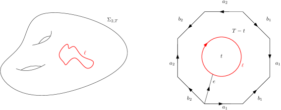
Figure 4: An contractible simple loop $\ell$ (on the left) and the oriented admissible graph associated to it (on the right).

If $\ell$ is an admissible simple loop of interior area $t$, then we can compute its Wilson loops expectation $W_{\ell}=\mathbb{E}[\mathrm{tr}(H_{\ell})]$, using Driver–Sengupta formula (3):

$$W_{\ell}=\frac{1}{Z_{N}(g,T)}\int_{G^{2g+1}}\mathrm{tr}(x)p_{t}(x^{-1})p_{T-t}(x[y_{1},z_{1}]\cdots[y_{g},z_{g}])\mathrm{d}x\prod_{i=1}^{g}\mathrm{d}y_{i}\mathrm{d}z_{i},$$ (39)

where $(p_{t})_{t\in\mathbb{R}_{+}}$ is the heat kernel on $G$.

We can also define the Wilson loop variance as the variance of Wilson loop functional – as tautological as it seems:

$$\mathrm{Var}[\mathrm{tr}(H_{\ell})]=\mathbb{E}[|\mathrm{tr}(H_{\ell})|^{2}]-|\mathbb{E}[\mathrm{tr}(H_{\ell})]|^{2}.$$

It appears that

$$\mathrm{Var}[\mathrm{tr}(H_{\ell})]=\mathbb{E}[\mathrm{tr}(H_{\ell})\overline{\mathrm{tr}(H_{\ell})}]-|\mathbb{E}[\mathrm{tr}(H_{\ell})]|^{2}=\mathbb{E}[\mathrm{tr}(H_{\ell})\mathrm{tr}(H_{\ell}^{*})]-|\mathbb{E}[\mathrm{tr}(H_{\ell})]|^{2},$$ (40)

so that the variance can be explicitly computed as long as we know the expectations $\mathbb{E}[\mathrm{tr}(H_{\ell})]$ and $\mathbb{E}[\mathrm{tr}(H_{\ell})\mathrm{tr}(H_{\ell}^{*})]$.

In order to use the theory of almost flat highest weights, we will need to express the Wilson loop expectation and variance in terms of irreducible representations. It will be based on the heat kernel decomposition (6) but also a few standard results from representation theory that we will recall afterwards. Our goal is to prove the following proposition.

Proposition 3.3 (Wilson loop expectation and variance).

Let $\Sigma_{g,T}$ be an orientable compact connected surface of genus $g\geqslant 1$ and of area $T$, $\ell$ be a contractible loop of interior area $t$, and $G={\mathrm{SU}}(N)$ or ${\mathrm{U}}(N)$ be the structure group. If we set $q=e^{-T/2}$, then we have the following formulas:

1. If $G={\mathrm{SU}}(N)$, then

   $$\mathbb{E}[\mathrm{tr}(H_{\ell})]= \frac{1}{NZ^{\prime}_{N}(g,T)}\sum_{\begin{subarray}{c}\lambda,\mu\in\widehat{{\mathrm{SU}}}(N)\\ \mu\nearrow\lambda\end{subarray}}\frac{q^{c^{\prime}_{2}(\mu)}}{(d_{\mu})^{2g-2}}\frac{d_{\lambda}}{d_{\mu}}e^{\frac{t}{2}(c^{\prime}_{2}(\mu)-c^{\prime}_{2}(\lambda))},$$ (41)

   $$\mathbb{E}[\mathrm{tr}(H_{\ell})\mathrm{tr}(H_{\ell}^{*})]= \frac{1}{N^{2}Z^{\prime}_{N}(g,T)}\sum_{\begin{subarray}{c}\lambda,\mu\in\widehat{{\mathrm{SU}}}(N)\\ \lambda\sim\mu\end{subarray}}\frac{q^{c^{\prime}_{2}(\mu)}}{(d_{\mu})^{2g-2}}\frac{d_{\lambda}}{d_{\mu}}e^{\frac{t}{2}(c^{\prime}_{2}(\mu)-c^{\prime}_{2}(\lambda))}.$$ (42)

2. If $G={\mathrm{U}}(N)$, then

   $$\mathbb{E}[\mathrm{tr}(H_{\ell})]= \frac{1}{NZ_{N}(g,T)}\sum_{\begin{subarray}{c}\lambda,\mu\in\widehat{{\mathrm{U}}}(N)\\ \mu\nearrow\lambda\end{subarray}}\frac{q^{c_{2}(\mu)}}{(d_{\mu})^{2g-2}}\frac{d_{\lambda}}{d_{\mu}}e^{\frac{t}{2}(c_{2}(\mu)-c_{2}(\lambda))},$$ (43)

   $$\mathbb{E}[\mathrm{tr}(H_{\ell})\mathrm{tr}(H_{\ell}^{*})]= \frac{1}{N^{2}Z_{N}(g,T)}\sum_{\begin{subarray}{c}\lambda,\mu\in\widehat{{\mathrm{U}}}(N)\\ \lambda\sim\mu\end{subarray}}\frac{q^{c_{2}(\mu)}}{(d_{\mu})^{2g-2}}\frac{d_{\lambda}}{d_{\mu}}e^{\frac{t}{2}(c_{2}(\mu)-c_{2}(\lambda))}.$$ (44)

Before we prove Proposition 3.3, let us introduce the following lemma, which enables to integrate Schur functions involving commutators.

Lemma 3.4.

Let $G$ be a compact group and $\mathrm{d}g$ its normalized Haar measure. If $(\rho,V)$ is an irreducible representation of $G$, we have

$$\int_{G^{2}}\chi_{\rho}(x[y,z])\mathrm{d}y\mathrm{d}z=\frac{\chi_{\rho}(x)}{d_{\rho}^{2}},\ \forall x\in G.$$ (45)

In order to prove Lemma 3.4, we need two intermediary propositions, which we will not prove because they are quite standard.

Proposition 3.5 ([Far08], Prop.5.2).

Let $G$ be a compact group, and $\mathrm{d}g$ its normalized Haar measure. For any irreducible representation $(\rho,V)$ of $G$, we have

$$\int_{G}\chi_{\rho}(xgyg^{-1})\mathrm{d}g=\frac{1}{d_{\rho}}\chi_{\rho}(x)\chi_{\rho}(y),\ \forall(x,y)\in G^{2}.$$

Proposition 3.6.

Let $G$ be a compact group and $(\rho,V)$, $(\pi,W)$ two irreducible representations of $G$. Then

$$\chi_{\rho}*\chi_{\pi}=\left\{\begin{array}[]{cc}\frac{\chi_{\rho}}{d_{\rho}}&\text{if }\rho\sim\pi,\\ 0&\text{otherwise.}\end{array}\right.$$

Proof of Lemma 3.4.

First, according to Proposition 3.5, we have for any $(x,y)\in G^{2}$ :

$$\int_{G}\chi_{\rho}(xyzy^{-1}z^{-1})\mathrm{d}z=\frac{1}{d_{\rho}}\chi_{\rho}(xy)\chi_{\rho}(y^{-1}).$$

If we integrate out $y\in G$ it appears that

$$\int_{G^{2}}\chi_{\rho}(x[y,z])\mathrm{d}y\mathrm{d}z=\frac{(\chi_{\rho}*\chi_{\rho})(x)}{d_{\rho}},$$

which yields (45) using Proposition 3.6. ∎

We now have all the tools to prove Proposition 3.3.

Proof of Proposition 3.3.

We will prove it in the case $G={\mathrm{U}}(N)$, the case $G={\mathrm{SU}}(N)$ being the same. Let us start from Eq. (39). We can decompose the heat kernels following (6):

$$W_{\ell}= \frac{1}{Z_{N}(g,T)}\sum_{\lambda,\mu\in\widehat{{\mathrm{U}}}(N)}d_{\lambda}d_{\mu}e^{-\frac{c_{2}(\lambda)t}{2}-\frac{c_{2}(\mu)(T-t)}{2}}$$

$$\int_{{\mathrm{U}}(N)^{2g+1}}\mathrm{tr}(x)s_{\lambda}(x^{-1})s_{\mu}(x[y_{1},z_{1}]\cdots[y_{g},z_{g}])\mathrm{d}x\prod_{i=1}^{g}\mathrm{d}y_{i}\mathrm{d}z_{i}.$$

We can then apply Lemma 3.4 $g$ times, which transforms the commutators into dimensions:

$$W_{\ell}= \frac{1}{Z_{N}(g,T)}\sum_{\lambda,\mu\in\widehat{{\mathrm{U}}}(N)}d_{\lambda}(d_{\mu})^{1-2g}e^{-\frac{c_{2}(\lambda)t}{2}-\frac{c_{2}(\mu)(T-t)}{2}}\int_{{\mathrm{U}}(N)}\mathrm{tr}(x)s_{\lambda}(x^{-1})s_{\mu}(x)\mathrm{d}x.$$

Then, using Pieri’s rule and the fact that $\mathrm{tr}=\frac{1}{N}\mathrm{Tr}$ gives

$$W_{\ell}= \frac{1}{Z_{N}(g,T)}\sum_{\lambda,\mu\in\widehat{{\mathrm{U}}}(N)}\frac{d_{\lambda}(d_{\mu})^{1-2g}}{N}e^{-\frac{c_{2}(\lambda)t}{2}-\frac{c_{2}(\mu)(T-t)}{2}}\sum_{\begin{subarray}{c}\nu\in\widehat{{\mathrm{U}}}(N)\\ \nu\searrow\mu\end{subarray}}\int_{{\mathrm{U}}(N)}s_{\lambda}(x^{-1})s_{\nu}(x)\mathrm{d}x.$$

If we set $q=e^{-T/2}$ and use the orthogonality relations of characters, it yields Eq. (43).

In the same manner as in Eq. (39), we can compute $\mathbb{E}[\mathrm{tr}(H_{\ell})\mathrm{tr}(H_{\ell}^{*})]$ as

$$\mathbb{E}[\mathrm{tr}(H_{\ell}) \mathrm{tr}(H_{\ell}^{*})]=$$

$$\frac{1}{Z_{N}(g,T)}\int_{{\mathrm{U}}(N)^{2g+1}}\mathrm{tr}(x)\mathrm{tr}(x^{-1})p_{t}(x^{-1})p_{T-t}(x[y_{1},z_{1}]\cdots[y_{g},z_{g}])\mathrm{d}x\prod_{i=1}^{g}\mathrm{d}y_{i}\mathrm{d}z_{i},$$

which can be rewritten, using the heat kernel decomposition, Lemma 3.4 and Lemma 3.2:

$$\mathbb{E}[\mathrm{tr}(H_{\ell})\mathrm{tr}(H_{\ell}^{*})]= \frac{1}{N^{2}Z_{N}(g,T)}\sum_{\lambda,\mu\in\widehat{{\mathrm{U}}}(N)}d_{\lambda}(d_{\mu})^{1-2g}e^{-\frac{c_{2}(\lambda)t}{2}-\frac{c_{2}(\mu)(T-t)}{2}}$$

$$\times\sum_{\begin{subarray}{c}\nu,\tau\in\widehat{{\mathrm{U}}}(N)\\ \nu\searrow\mu,\tau\searrow\lambda\end{subarray}}\int_{{\mathrm{U}}(N)}s_{\tau}(x^{-1})s_{\nu}(x)\mathrm{d}x.$$

Setting $q=e^{-T/2}$ as before and using the orthogonality of Schur functions, we obtain Eq. (44) as expected. ∎

It is now time to state the main results of this section, which give the limits of the Wilson loop expectation and variance for a simple loop in a closed topological disk.

Theorem 3.7.

Let $\Sigma_{g,T}$ be an orientable compact connected surface of genus $g\geqslant 1$ and of area $T$, $\ell$ be a contractible simple loop of interior area $t$, and $G={\mathrm{SU}}(N)$ or ${\mathrm{U}}(N)$ be the structure group. The associated Wilson loop expectation converges, as $N\to\infty$, and its limit is

$$\lim_{N\to\infty}\mathbb{E}[\mathrm{tr}(H_{\ell})]=e^{-\frac{t}{2}}.$$ (46)

Note that the limit does actually not depend on the genus of the surface, as long as it is greater or equal to $1$. The value of the limit is the same as in the plane. The result about the variance is the following.

Theorem 3.8.

Let $\Sigma_{g,T}$ be an orientable compact connected surface of genus $g\geqslant 1$ and of area $T$, $\ell$ be a contractible simple loop of interior area $t$, and $G={\mathrm{SU}}(N)$ or ${\mathrm{U}}(N)$ be the structure group. The associated Wilson loop variance satisfies the following limit:

$$\lim_{N\to\infty}\mathrm{Var}[\mathrm{tr}(H_{\ell})]=0.$$ (47)

Theorems 3.7 and 3.8 imply that the Wilson loops $W_{\ell}$ converge in probability to the limit given by (46); this result was obtained in [DL22] using probabilistic arguments, but we find interesting to provide a purely representation-theoretic proof. The proof will still be partly based on a previous fundamental result: the convergence of partition functions.

Theorem 3.9 ([Lem21]).

Let $\Sigma_{g,T}$ be an orientable surface of genus $g\geqslant 1$ and area $T\geqslant 0$. For $t\in(0,+\infty)$, set $\theta(t)=\sum_{n\in{\mathbb{Z}}}e^{-tn^{2}}$ and $q_{t}=e^{-\tfrac{t}{2}}$, and for $s\in(0,1)$, set $\phi(s)=\prod_{m=1}^{\infty}(1-s^{m})$.

1. If $g\geqslant 2$ and $T>0$:

   $$\lim_{N\to\infty}Z_{N}(g,T)=\theta(\tfrac{T}{2})\ \text{ and }\ \lim_{N\to\infty}Z^{\prime}_{N}(g,T)=1.$$ (48)

2. If $g\geqslant 2$ and $T=0$:

   $$\lim_{N\to\infty}Z^{\prime}_{N}(g,0)=1.$$ (49)

3. If $g=1$ and $T>0$:

   $$\lim_{N\to\infty}Z_{N}(1,T)=\frac{\theta(\tfrac{T}{2})}{\phi(q)^{2}}\ \text{ and }\ \lim_{N\to\infty}Z^{\prime}_{N}(1,T)=\frac{1}{\phi(q)^{2}}.$$ (50)

3.3 Proofs using the almost flat highest weights

3.3.1 Branching rules

Before proving Theorem 3.7, we still have to discuss a bit about branching rules. Indeed, in (41) (resp. (43)), a sum over $\lambda\searrow\mu$ appears, with $\lambda$ and $\mu$ being highest weights of ${\mathrm{SU}}(N)$ (resp. ${\mathrm{U}}(N)$). We will show how this branching is transformed in the decomposition $\lambda=\lambda_{N}(\alpha,\beta,n)$.

Proposition 3.10.

Let $\alpha=(\alpha_{1}\geqslant\cdots\geqslant\alpha_{r})$, $\beta=(\beta_{1}\geqslant\cdots\geqslant\beta_{s})$, $\alpha^{\prime}=(\alpha^{\prime}_{1}\geqslant\cdots\geqslant\alpha^{\prime}_{r^{\prime}})$ and $\beta^{\prime}=(\beta^{\prime}_{1}\geqslant\cdots\geqslant\beta^{\prime}_{s^{\prime}})$ be integer partitions, and $(n,n^{\prime},N)\in{\mathbb{Z}}^{3}$ three integers such that $N\geqslant\max(r+s,r^{\prime}+s^{\prime})$. Then the following assertions are equivalent:

1. $\lambda_{N}(\alpha^{\prime},\beta^{\prime},n^{\prime})\searrow\lambda_{N}(\alpha,\beta,n)$,

2. ($\alpha^{\prime}\searrow\alpha$, $\beta^{\prime}=\beta$ and $n^{\prime}=n$)  or  ($\beta^{\prime}\nearrow\beta$, $\alpha^{\prime}=\alpha$ and $n^{\prime}=n$).

Proof.

In order to see the equivalence, recall the construction of $\lambda_{N}(\alpha,\beta,n)$ given in (9):

$$\lambda_{N}(\alpha,\beta,n)=(\alpha_{1}+n,\ldots,\alpha_{r}+n,\underbrace{n,\ldots,n}_{N-r-s},n-\beta_{s},\ldots,n-\beta_{1})=(\lambda_{1},\ldots,\lambda_{N}).$$

The only way of having $\lambda_{N}(\alpha^{\prime},\beta^{\prime},n^{\prime})\searrow\lambda_{N}(\alpha,\beta,n)$ is to increment a coefficient $\lambda_{i}$ such that $\lambda_{i}>\lambda_{i+1}$. It clearly excludes the coefficients $\lambda_{r+1},\ldots,\lambda_{r+s}$. Two only ways remain: either we increment one of the coefficients $\lambda_{1},\ldots,\lambda_{r}$, or we increment one of the coefficients $\lambda_{r+s+1},\ldots,\lambda_{N}$. The first case corresponds to $\alpha^{\prime}\searrow\alpha$ and the second one to $\beta^{\prime}\nearrow\beta$ (while leaving the other parameters unchanged), according to the description of the coefficients in terms of $\alpha,\beta$ and $n$. The equivalence follows immediately. ∎

The main consequence of this proposition, combined with (21) and (22), is that for $N$ large enough,

$$\{(\lambda,\mu)\in\widehat{{\mathrm{SU}}}(N)\times\Lambda_{N,1}^{\gamma}:\ \lambda\searrow\mu\}$$

splits into two disjoint sets

$$\{(\lambda_{N}(\alpha^{\prime},\beta),\lambda_{N}(\alpha,\beta)):\ |\alpha|\leqslant N^{\gamma},|\beta|\leqslant N^{\gamma},\alpha^{\prime}\searrow\alpha\}$$

and

$$\{(\lambda_{N}(\alpha,\beta^{\prime}),\lambda_{N}(\alpha,\beta)):\ |\alpha|\leqslant N^{\gamma},|\beta|\leqslant N^{\gamma},\beta^{\prime}\nearrow\beta\}.$$

From (22) we also have that, for $N$ large enough,

$$\{(\lambda,\mu)\in\widehat{{\mathrm{U}}}(N)\times\Omega_{N,1}^{\gamma}:\ \lambda\searrow\mu\}$$

splits into

$$\{(\lambda_{N}(\alpha^{\prime},\beta,n),\lambda_{N}(\alpha,\beta,n)):\ |\alpha|\leqslant N^{\gamma},|\beta|\leqslant N^{\gamma},\alpha^{\prime}\searrow\alpha,n\in{\mathbb{Z}}\}$$

and

$$\{(\lambda_{N}(\alpha,\beta^{\prime},n),\lambda_{N}(\alpha,\beta,n)):\ |\alpha|\leqslant N^{\gamma},|\beta|\leqslant N^{\gamma},\beta^{\prime}\nearrow\beta,n\in{\mathbb{Z}}\}.$$

The main advantage of these decompositions is that we make fully use of Proposition 2.4 that uses branching over partitions rather than highest weights. However, using Proposition 2.5 will somehow convert dimensions of representations of ${\mathrm{U}}(N)$ or ${\mathrm{SU}}(N)$ into dimensions of representations of $\mathfrak{S}_{n}$ with some integer $n$. We will therefore need the following branching rules.

Proposition 3.11.

Let $\lambda\vdash n$ for any positive integer $n$. We have

$$\sum_{\begin{subarray}{c}\mu\vdash(n+1)\\ \mu\searrow\lambda\end{subarray}}\frac{d^{\mu}}{(n+1)d^{\lambda}}=1,$$ (51)

and

$$\sum_{\begin{subarray}{c}\mu\vdash(n-1)\\ \mu\nearrow\lambda\end{subarray}}\frac{d^{\mu}}{d^{\lambda}}=1.$$ (52)

Proof.

Let us recall the so-called branching rules on $\mathfrak{S}_{n}$, cf. [Sag01] for example:

$$\chi^{\lambda}\uparrow^{\mathfrak{S}_{n+1}}=\sum_{\begin{subarray}{c}\mu\vdash(n+1)\\ \mu\searrow\lambda\end{subarray}}\chi^{\mu},$$

and

$$\chi^{\lambda}\downarrow_{\mathfrak{S}_{n-1}}=\sum_{\begin{subarray}{c}\mu\vdash(n-1)\\ \mu\nearrow\lambda\end{subarray}}\chi^{\mu}.$$

As the character of a restricted representation is equal to the restriction of the character, the second branching rule directly implies (52). For the character of an induced representation we have the following result [FH91, Eq.(3.18)]: if $G$ is a finite group and $H$ a subgroup of $G$, then for any character $\chi$ of a representation of $H$ we have

$$\chi\uparrow^{G}(g)=\frac{1}{|H|}\sum_{\begin{subarray}{c}x\in G\\ xgx^{-1}\in H\end{subarray}}\chi(xgx^{-1}),\ \forall g\in G.$$

If we apply this formula to $G=\mathfrak{S}_{n+1}$, $H=\mathfrak{S}_{n}$, $\chi=\chi^{\lambda}$ and $g=1$ we get (51) as expected. ∎

3.3.2 Asymptotics of the expectation

We can now turn to the proof of Theorem 3.7. We will split it into one dedicated to ${\mathrm{SU}}(N)$ and one dedicated to ${\mathrm{U}}(N)$, as the proofs are slightly different.

Proof of Theorem 3.7 in the special unitary case.

Let $\gamma\in(0,\frac{1}{3})$ be a fixed real number. For any $i\in\{1,2,3,4\}$ we define $\mathbb{E}_{i}^{\gamma}[\mathrm{tr}(H_{\ell})]$ as follows:

$$\mathbb{E}_{i}^{\gamma}[\mathrm{tr}(H_{\ell})]=\frac{1}{NZ^{\prime}_{N}(g,T)}\sum_{\mu\in\Lambda_{N,i}^{\gamma}}\frac{q^{c^{\prime}_{2}(\mu)}}{(d_{\mu})^{2g-2}}\sum_{\begin{subarray}{c}\lambda\in\widehat{{\mathrm{SU}}}(N)\\ \lambda\searrow\mu\end{subarray}}\frac{d_{\lambda}}{d_{\mu}}e^{\frac{t}{2}(c^{\prime}_{2}(\mu)-c^{\prime}_{2}(\lambda))},$$

with the sets $\Lambda_{N,i}^{\gamma}$ being as in (18).

From Equation (41) and the definition of each $\Lambda_{N,i}^{\gamma}$ we have $\mathbb{E}[\mathrm{tr}(H_{\ell})]=\sum_{i=1}^{4}\mathbb{E}_{i}^{\gamma}[\mathrm{tr}(H_{\ell})]$. We will show first that

$$\lim_{N\to\infty}\mathbb{E}_{1}^{\gamma}[\mathrm{tr}(H_{\ell})]=e^{-t/2},$$

and then that for $2\leqslant i\leqslant 4$,

$$\lim_{N\to\infty}\mathbb{E}_{i}^{\gamma}[\mathrm{tr}(H_{\ell})]=0,$$

which will imply Equation (46).

From Equation (21) we have, for $N$ large enough,

$$\mathbb{E}_{1}^{\gamma}[\mathrm{tr}(H_{\ell})]=\frac{1}{NZ^{\prime}_{N}(g,T)}\sum_{|\alpha|,|\beta|\leqslant N^{\gamma}}\frac{q^{c^{\prime}_{2}(\lambda_{N}(\alpha,\beta))}}{(d_{\lambda_{N}(\alpha,\beta)})^{2g-2}}\sum_{\begin{subarray}{c}\lambda\in\widehat{{\mathrm{SU}}}(N)\\ \lambda\searrow\lambda_{N}(\alpha,\beta)\end{subarray}}\frac{d_{\lambda}}{d_{\lambda_{N}(\alpha,\beta)}}e^{\frac{t}{2}(c^{\prime}_{2}(\lambda_{N}(\alpha,\beta))-c^{\prime}_{2}(\lambda))}.$$

Furthermore, we can notice that adding a box to $\lambda_{N}(\alpha,\beta)$ is equivalent to adding a box to the partition $\alpha$ to get $\alpha^{\prime}\searrow\alpha$ or removing one from the partition $\beta$ to get $\beta^{\prime}\nearrow\beta$ such that $\alpha^{\prime}$ or $\beta^{\prime}$ is another partition. It means that

$$\begin{split}\mathbb{E}_{1}^{\gamma}[\mathrm{tr}(H_{\ell})]=&\frac{1}{NZ^{\prime}_{N}(g,T)}\sum_{|\alpha|,|\beta|\leqslant N^{\gamma}}\frac{q^{c^{\prime}_{2}(\lambda_{N}(\alpha,\beta))}}{(d_{\lambda_{N}(\alpha,\beta)})^{2g-2}}\\ &\times\left(\sum_{\alpha^{\prime}\searrow\alpha}\frac{d_{\lambda_{N}(\alpha^{\prime},\beta)}}{d_{\lambda_{N}(\alpha,\beta)}}e^{\frac{t}{2}(c^{\prime}_{2}(\lambda_{N}(\alpha,\beta))-c^{\prime}_{2}({\lambda_{N}(\alpha^{\prime},\beta)}))}\right.\\ &\hskip 56.9055pt+\left.\sum_{\beta^{\prime}\nearrow\beta}\frac{d_{\lambda_{N}(\alpha,\beta^{\prime})}}{d_{\lambda_{N}(\alpha,\beta)}}e^{\frac{t}{2}(c^{\prime}_{2}(\lambda_{N}(\alpha,\beta))-c^{\prime}_{2}({\lambda_{N}(\alpha,\beta^{\prime})}))}\right).\end{split}$$ (53)

We will first control the differences of Casimir numbers, then the ratios of dimensions, and show that only the sum over $\alpha^{\prime}\searrow\alpha$ contributes to the large $N$ limit. From (20) we obtain that for any $\alpha$ and $\beta$ such that $|\alpha|,|\beta|\leqslant N^{\gamma}$,

$$-1-16N^{2\gamma-1}\leqslant c^{\prime}_{2}(\lambda_{N}(\alpha,\beta))-c^{\prime}_{2}(\lambda_{N}(\alpha^{\prime},\beta))\leqslant-1+16N^{2\gamma-1},\ \forall\alpha^{\prime}\searrow\alpha$$

and

$$1-16N^{2\gamma-1}\leqslant c^{\prime}_{2}(\lambda_{N}(\alpha,\beta))-c^{\prime}_{2}(\lambda_{N}(\alpha,\beta^{\prime}))\leqslant 1+16N^{2\gamma-1},\ \forall\beta^{\prime}\nearrow\beta.$$

We obtain the following estimation for $\mathbb{E}_{1}^{\gamma}[\mathrm{tr}(H_{\ell})]$:

$$\begin{split}\mathbb{E}_{1}^{\gamma}[\mathrm{tr}(H_{\ell})]=&\frac{e^{\varepsilon(N,\gamma)}}{Z^{\prime}_{N}(g,T)}\sum_{|\alpha|,|\beta|\leqslant N^{\gamma}}\frac{q^{|\alpha|+|\beta|}}{(d_{\lambda_{N}(\alpha,\beta)})^{2g-2}}\left(\frac{e^{-\frac{t}{2}}}{N}\sum_{\alpha^{\prime}\searrow\alpha}\frac{d_{\lambda_{N}(\alpha^{\prime},\beta)}}{d_{\lambda_{N}(\alpha,\beta)}}+\frac{e^{\frac{t}{2}}}{N}\sum_{\beta^{\prime}\nearrow\beta}\frac{d_{\lambda_{N}(\alpha,\beta^{\prime})}}{d_{\lambda_{N}(\alpha,\beta)}}\right),\end{split}$$ (54)

with

$$|\varepsilon(N,\gamma)|\leqslant(4T+8t)N^{2\gamma-1}.$$

Using Proposition 2.5 and the fact that for any $x\in(0,\tfrac{1}{4})$

$$\frac{1}{1-2x}\leqslant 1+4x\hskip 14.22636pt\text{ and }\hskip 14.22636pt\frac{1}{1+2x}\geqslant 1-4x,$$

we have for any $\alpha^{\prime}\searrow\alpha$ and $N$ large enough

$$\frac{d_{\lambda_{N}(\alpha^{\prime},\beta)}}{d_{\lambda_{N}(\alpha,\beta)}}\leqslant\frac{Nd^{\alpha^{\prime}}}{(|\alpha|+1)d^{\alpha}}(1+24N^{3\gamma-1})(1+48N^{3\gamma-1})\leqslant\frac{Nd^{\alpha^{\prime}}}{(|\alpha|+1)d^{\alpha}}(1+144N^{3\gamma-1})$$

and

$$\frac{d_{\lambda_{N}(\alpha^{\prime},\beta)}}{d_{\lambda_{N}(\alpha,\beta)}}\geqslant\frac{Nd^{\alpha^{\prime}}}{(|\alpha|+1)d^{\alpha}}(1-144N^{3\gamma-1}).$$

Combined with Proposition 3.11 these equations yield

$$1-144N^{3\gamma-1}\leqslant\frac{1}{N}\sum_{\alpha^{\prime}\searrow\alpha}\frac{d_{\lambda_{N}(\alpha^{\prime},\beta)}}{d_{\lambda_{N}(\alpha,\beta)}}\leqslant 1+144N^{3\gamma-1}.$$ (55)

With similar arguments we also have, because $|\beta|\leqslant N^{\gamma}$:

$$0\leqslant\frac{1}{N}\sum_{\beta^{\prime}\nearrow\beta}\frac{d_{\lambda_{N}(\alpha,\beta^{\prime})}}{d_{\lambda_{N}(\alpha,\beta)}}\leqslant\frac{|\beta|}{N^{2}}(1+144N^{3\gamma-1})\leqslant 37N^{\gamma-2}.$$ (56)

Combining this with (54) we find

$$\mathbb{E}_{1}^{\gamma}[\mathrm{tr}(H_{\ell})]=e^{-\frac{t}{2}}\eta(N,\gamma)\frac{e^{\varepsilon(N,\gamma)}}{Z^{\prime}_{N}(g,T)}\sum_{|\alpha|,|\beta|\leqslant N^{\gamma}}\frac{q^{|\alpha|+|\beta|}}{(d_{\lambda_{N}(\alpha,\beta)})^{2g-2}},$$ (57)

with

$$1-144N^{2\gamma-1}\leqslant\eta(N,\gamma)\leqslant 1+144N^{3\gamma-1}+37e^{t}N^{\gamma-2}.$$

If we let $N\to\infty$, the remaining sum has the same limit as $Z^{\prime}_{N}(g,T)$, using similar arguments as in the proof of Theorem 3.9. Moreover, $\varepsilon(N,\gamma)$ tends to $0$ and $\eta(N,\gamma)$ to $1$. From all of this we can deduce that $\lim_{N\to\infty}\mathbb{E}_{1}^{\gamma}[\mathrm{tr}(H_{\ell})]=e^{-\frac{t}{2}}$.

Now we have to show that the other $\mathbb{E}_{i}^{\gamma}$ all tend to $0$ when $N\to\infty$. We have

$$\mathbb{E}_{i}^{\gamma}[\mathrm{tr}(H_{\ell})]=\frac{1}{NZ^{\prime}_{N}(g,T)}\sum_{\mu\in\Lambda_{N,i}^{\gamma}}\frac{q^{c^{\prime}_{2}(\mu)}}{(d_{\mu})^{2g-2}}\sum_{\begin{subarray}{c}\lambda\in\widehat{{\mathrm{SU}}}(N)\\ \lambda\searrow\mu\end{subarray}}\frac{d_{\lambda}}{d_{\mu}}e^{\frac{t}{2}(c^{\prime}_{2}(\mu)-c^{\prime}_{2}(\lambda))}.$$

Using Proposition 2.3, if we set $\alpha=\alpha_{\mu}$ and $\beta=\beta_{\mu}$, we have the following inequality for $N$ large enough:

$$\mathbb{E}_{i}^{\gamma}[\mathrm{tr}(H_{\ell})]\leqslant\frac{1}{NZ^{\prime}_{N}(g,T)}\sum_{\mu\in\Lambda_{N,i}^{\gamma}}\frac{e^{-\frac{T}{8}(|\alpha|+|\beta|)+t}}{(d_{\mu})^{2g-2}}\sum_{\begin{subarray}{c}\lambda\in\widehat{{\mathrm{SU}}}(N)\\ \lambda\searrow\mu\end{subarray}}\frac{d_{\lambda}}{d_{\mu}}.$$

Furthermore, using (33) we have

$$\sum_{\begin{subarray}{c}\lambda\in\widehat{{\mathrm{SU}}}(N)\\ \lambda\searrow\mu\end{subarray}}\frac{d_{\lambda}}{d_{\mu}}=\mathrm{Tr}(I_{N})=N,$$

therefore

$$\mathbb{E}_{i}^{\gamma}[\mathrm{tr}(H_{\ell})]\leqslant\frac{1}{Z^{\prime}_{N}(g,T)}\sum_{\mu\in\Lambda_{N,i}^{\gamma}}\frac{e^{-\frac{T}{8}(|\alpha|+|\beta|)+t}}{(d_{\mu})^{2g-2}}\leqslant\frac{1}{Z^{\prime}_{N}(g,T)}\sum_{\mu\in\Lambda_{N,i}^{\gamma}}e^{-\frac{T}{8}(|\alpha|+|\beta|)+t},$$

where in the second inequality we used the fact that for any $\mu\in\Lambda_{N,i}^{\gamma}$, $d_{\mu}\geqslant 1$.

From now on, we will set $i=2$, but the arguments will be similar for $i=3$ and $i=4$. For $N$ large enough, we have

$$\mathbb{E}_{2}^{\gamma}[\mathrm{tr}(H_{\ell})]\leqslant \frac{e^{t}}{Z^{\prime}_{N}(g,T)}\sum_{|\alpha|>N^{\gamma},|\beta|\leqslant N^{\gamma}}e^{-\frac{T}{8}(|\alpha|+|\beta|)+t}$$

$$= \frac{e^{t}}{Z^{\prime}_{N}(g,T)}\sum_{|\alpha|>N^{\gamma}}e^{-\frac{T}{8}|\alpha|}\sum_{|\beta|\leqslant N^{\gamma}}e^{-\frac{T}{8}|\beta|}.$$

The fraction $\frac{e^{t}}{Z^{\prime}_{N}(g,T)}$ is bounded because $(Z^{\prime}_{N}(g,T))_{N\geqslant 1}$ is a convergent sequence, see [Lem21]; the first sum converges to $0$ as the remainder of the convergent series defining the generating function of partitions. The second sum is bounded as the partial sum of a similar generating function. We obtain that $\mathbb{E}_{2}^{\gamma}[\mathrm{tr}(H_{\ell})]\to 0$ as $N\to\infty$. We have the same convergence for $i=3$ and $i=4$ and the result follows. ∎

Proof of Theorem 3.7 in the unitary case.

Let $\gamma\in(0,\tfrac{1}{3})$ be a fixed real number. As in the special unitary case, we define for $1\leqslant i\leqslant 4$ the quantity $\mathbb{E}_{i}^{\gamma}[\mathrm{tr}(H_{\ell})]$ as

$$\mathbb{E}_{i}^{\gamma}[\mathrm{tr}(H_{\ell})]=\frac{1}{NZ_{N}(g,T)}\sum_{\mu\in\Omega_{N,i}^{\gamma}}\frac{q^{c_{2}(\mu)}}{(d_{\mu})^{2g-2}}\sum_{\begin{subarray}{c}\lambda\in\widehat{{\mathrm{U}}}(N)\\ \lambda\searrow\mu\end{subarray}}\frac{d_{\lambda}}{d_{\mu}}e^{\frac{t}{2}(c_{2}(\mu)-c_{2}(\lambda))}.$$ (58)

As we have seen right after Proposition 3.10, we have for $N$ large enough

$$\mathbb{E}_{1}^{\gamma}[\mathrm{tr}(H_{\ell})]= \frac{1}{Z_{N}(g,T)}\sum_{|\alpha|,|\beta|\leqslant N^{\gamma}}\sum_{n\in{\mathbb{Z}}}\frac{q^{c_{2}(\lambda_{N}(\alpha,\beta,n))}}{(d_{\lambda_{N}(\alpha,\beta,n)})^{2g-2}}$$

$$\times\left(\frac{1}{N}\sum_{\alpha^{\prime}\searrow\alpha}\frac{d_{\lambda_{N}(\alpha^{\prime},\beta,n)}}{d_{\lambda_{N}(\alpha,\beta,n)}}e^{\frac{t}{2}(c_{2}(\lambda_{N}(\alpha,\beta,n))-c_{2}(\lambda_{N}(\alpha^{\prime},\beta,n)))}\right.$$

$$\hskip 56.9055pt+\left.\frac{1}{N}\sum_{\beta^{\prime}\nearrow\beta}\frac{d_{\lambda_{N}(\alpha,\beta^{\prime},n)}}{d_{\lambda_{N}(\alpha,\beta,n)}}e^{\frac{t}{2}(c_{2}(\lambda_{N}(\alpha,\beta,n))-c_{2}(\lambda_{N}(\alpha,\beta^{\prime},n)))}\right).$$

Let us introduce two intermediary quantities, depending on $\alpha$, $\beta$ and $n$:

$$A_{N}(\alpha,\beta,n)=\frac{1}{N}\sum_{\alpha^{\prime}\searrow\alpha}\frac{d_{\lambda_{N}(\alpha^{\prime},\beta,n)}}{d_{\lambda_{N}(\alpha,\beta,n)}}\sum_{n\in{\mathbb{Z}}}e^{\frac{t}{2}(c_{2}(\lambda_{N}(\alpha,\beta,n))-c_{2}({\lambda_{N}(\alpha^{\prime},\beta,n)}))},$$

$$B_{N}(\alpha,\beta,n)=\frac{1}{N}\sum_{\begin{subarray}{c}\beta^{\prime}\nearrow\beta\end{subarray}}\frac{d_{\lambda_{N}(\alpha,\beta^{\prime},n)}}{d_{\lambda_{N}(\alpha,\beta,n)}}\sum_{n\in{\mathbb{Z}}}e^{\frac{t}{2}(c_{2}(\lambda_{N}(\alpha,\beta,n))-c_{2}({\lambda_{N}(\alpha,\beta^{\prime},n)}))}.$$

We will show that $A_{N}(\alpha,\beta,n)$ produces the limit we are trying to get, and that $B_{N}(\alpha,\beta,n)$ do not contribute to this limit. Let us first consider $A_{N}(\alpha,\beta,n)$ and use Proposition 2.4: from (16) and the fact that for any $1\leqslant i\leqslant N$

$$-N^{\gamma-1}\leqslant\frac{\alpha_{i}+\beta_{1}+1-i}{N}\leqslant N^{\gamma-1}+\frac{1}{N}\leqslant 2N^{\gamma-1},$$

we deduce

$$c_{2}(\lambda_{N}(\alpha,\beta,n))-c_{2}(\lambda_{N}(\alpha^{\prime},\beta,n))=-1-\frac{2n}{N}+\varepsilon_{1}(N,\gamma)$$

with $|\varepsilon_{1}(N,\gamma)|\leqslant 2N^{\gamma-1}$. Combining this estimation with Equation (55) yields

$$A_{N}(\alpha,\beta,n)=e^{-\frac{t}{2}+\varepsilon_{1}(N,\gamma)}(1+\eta_{1}(N,\gamma))e^{-\frac{tn}{N}},$$

with $|\eta_{1}(N,\gamma)|\leqslant 144N^{2\gamma-1}$. Analogously, we have from (17) and (56)

$$B_{N}(\alpha,\beta,n)=e^{\frac{t}{2}+\varepsilon_{2}(N,\gamma)}\eta_{2}(N,\gamma)e^{-\frac{tn}{N}},$$

with $|\varepsilon_{2}(N,\gamma)|\leqslant 0$ and $|\eta_{2}(N,\gamma)|\leqslant 36N^{\gamma-2}$. In particular, we have

$$\mathbb{E}_{1}^{\gamma}[\mathrm{tr}(H_{\ell})]=\frac{C_{N}}{Z_{N}(g,T)}\left(e^{-\frac{t}{2}+\varepsilon_{1}(N,\gamma)}(1+\eta_{1}(N,\gamma))+e^{\frac{t}{2}+\varepsilon_{2}(N,\gamma)}\eta_{2}(N,\gamma)\right),$$ (59)

with

$$C_{N}=\sum_{n\in{\mathbb{Z}}}e^{-\frac{tn}{N}}\sum_{|\alpha|,|\beta|\leqslant N^{\gamma}}\frac{q^{c_{2}(\lambda_{N}(\alpha,\beta,n))}}{(d_{\lambda_{N}(\alpha,\beta,n)})^{2g-2}}.$$

We would like to show that $\lim_{N\to\infty}C_{N}=\lim_{N\to\infty}Z_{N}(g,T)$. From the definitions of Casimir numbers, we have

$$c_{2}(\lambda+n)=c_{2}^{\prime}(\lambda)+\bigg{(}n+\frac{|\lambda|}{N}\bigg{)}^{2},$$

and it follows that

$$C_{N}=\sum_{|\alpha|,|\beta|\leqslant N^{\gamma}}\left(\sum_{n\in{\mathbb{Z}}}q^{\left(n+\frac{|\alpha|-|\beta|}{N}\right)^{2}+\frac{2tn}{TN}}\right)\frac{q^{c^{\prime}_{2}(\lambda_{N}(\alpha,\beta))}}{(d_{\lambda_{N}(\alpha,\beta)})^{2g-2}}.$$

For any $\alpha$ and $\beta$ such that $|\alpha|,|\beta|\leqslant N^{\gamma}$, we have $\big{|}|\alpha_{\lambda}|-|\beta_{\lambda}|\big{|}\leqslant|\alpha_{\lambda}|+|\beta_{\lambda}|\leqslant 2N^{\gamma}$, so that

$$n^{2}-4nN^{\gamma-1}\leqslant\left(n+\frac{|\alpha_{\lambda}|-|\beta_{\lambda}|}{N}\right)^{2}\leqslant n^{2}+4nN^{\gamma-1}+4N^{2\gamma-2}.$$ (60)

It follows that

$$n^{2}-n\left(4N^{\gamma-1}-\frac{2t}{TN}\right)\leqslant\left(n+\frac{|\alpha|-|\beta|}{N}\right)^{2}+\frac{2tn}{TN}\leqslant n^{2}+n\left(4N^{\gamma-1}+\frac{2t}{TN}\right)+4N^{2\gamma-2}.$$

We can plug these estimates in the sums to bound $C_{N}$:

$$\left(\sum_{n\in{\mathbb{Z}}}q^{n^{2}+n\left(4N^{\gamma-1}+\frac{2t}{TN}\right)+4N^{2\gamma-2}}\right)\sum_{|\alpha|,|\beta|\leqslant N^{\gamma}}\frac{q^{c^{\prime}_{2}(\lambda_{N}(\alpha,\beta))}}{(d_{\lambda_{N}(\alpha,\beta)})^{2g-2}}\leqslant C_{N},$$

and

$$C_{N}\leqslant\left(\sum_{n\in{\mathbb{Z}}}q^{n^{2}-n\left(4N^{\gamma-1}-\frac{2t}{TN}\right)}\right)\sum_{|\alpha|,|\beta|\leqslant N^{\gamma}}\frac{q^{c^{\prime}_{2}(\lambda_{N}(\alpha,\beta))}}{(d_{\lambda_{N}(\alpha,\beta)})^{2g-2}}.$$

The quantity $\sum_{|\alpha|,|\beta|\leqslant N^{\gamma}}\frac{q^{c^{\prime}_{2}(\lambda_{N}(\alpha,\beta))}}{(d_{\lambda_{N}(\alpha,\beta)})^{2g-2}}$ has the same limit as $Z^{\prime}_{N}(g,T)$ as in the proof of Theorem 3.9. Moreover we have, by dominated convergence,

$$\lim_{N\to\infty}\sum_{n\in{\mathbb{Z}}}q^{n^{2}-n\left(4N^{\gamma-1}-\frac{2t}{TN}\right)}=\lim_{N\to\infty}\sum_{n\in{\mathbb{Z}}}q^{n^{2}+n\left(4N^{\gamma-1}+\frac{2t}{TN}\right)+4N^{2\gamma-2}}=\sum_{n\in{\mathbb{Z}}}q^{n^{2}},$$

therefore

$$\lim_{N\to\infty}C_{N}=\sum_{n\in{\mathbb{Z}}}q^{n^{2}}\lim_{N\to\infty}Z^{\prime}_{N}(g,T)=Z_{N}(g,T).$$

Plugging this limit into (59) and using the estimates of $\varepsilon_{1}(N,\gamma)$, $\varepsilon_{2}(N,\gamma)$, $\eta_{1}(N,\gamma)$ and $\eta_{2}(N,\gamma)$, we finally get

$$\lim_{N\to\infty}\mathbb{E}_{1}^{\gamma}[\mathrm{tr}(H_{\ell})]=e^{-\frac{t}{2}}.$$

Now we have to show that the other $\mathbb{E}_{i}^{\gamma}$ all tend to $0$ when $N\to\infty$. We will need the following estimations, which are direct consequences of (16): if $\alpha,\beta,\alpha^{\prime},\beta^{\prime}$ are partitions such that $\alpha^{\prime}\searrow\alpha$ and $\beta^{\prime}\nearrow\beta$, then for any $n\in{\mathbb{Z}}$ we have

$$c_{2}(\lambda_{N}(\alpha,\beta,n))-c_{2}(\lambda_{N}(\alpha^{\prime},\beta,n))\leqslant 1-\frac{2n}{N}$$

and

$$c_{2}(\lambda_{N}(\alpha,\beta,n))-c_{2}(\lambda_{N}(\alpha,\beta^{\prime},n))\leqslant 1-\frac{2n}{N}.$$

In particular, combined with Proposition 3.10, these estimations imply that for any $(\lambda,\mu)\in\widehat{{\mathrm{U}}}(N)^{2}$ such that $\lambda\searrow\mu$,

$$c_{2}(\mu)-c_{2}(\lambda)\leqslant 1-\frac{2n}{N},$$ (61)

with $n=n_{\mu}$. Recall that from (33) we have

$$\sum_{\begin{subarray}{c}\lambda\in\widehat{{\mathrm{U}}}(N)\\ \lambda\searrow\mu\end{subarray}}\frac{d_{\lambda}}{d_{\mu}}=N.$$

If we combine these results with (58), we get the following estimation:

$$0\leqslant\mathbb{E}_{i}^{\gamma}[\mathrm{tr}(H_{\ell})]\leqslant\frac{e^{\frac{t}{2}}}{Z_{N}(g,T)}\sum_{\mu\in\Omega_{N,i}^{\gamma}}\frac{q^{c_{2}(\mu)+\frac{2tn_{\mu}}{TN}}}{(d_{\mu})^{2g-2}}.$$ (62)

Now let us specialize our computation to a given $i$. We will do it for $i=2$, the other cases being similar. We have

$$0\leqslant\mathbb{E}_{2}^{\gamma}[\mathrm{tr}(H_{\ell})]\leqslant\frac{C_{N,2}}{Z_{N}(g,T)},$$

with

$$C_{N,2}=e^{\frac{t}{2}}\sum_{|\alpha|>N^{\gamma},|\beta|\leqslant N^{\gamma}}\sum_{n\in{\mathbb{Z}}}\frac{q^{c^{\prime}_{2}(\lambda_{N}(\alpha,\beta))+\left(n+\frac{|\alpha|-|\beta|}{N}\right)^{2}+\frac{2tn}{TN}}}{(d_{\lambda_{N}(\alpha,\beta)})^{2g-2}}.$$

Recall that for any $\alpha$ and $\beta$ we have $d_{\lambda_{N}(\alpha,\beta)}\geqslant 1$. Besides, from (14) we have $c^{\prime}_{2}(\lambda_{N}(\alpha,\beta))\geqslant\tfrac{1}{2}|\alpha|+|\beta|$, and we also have the following estimation:

$$-\frac{T}{2}\left(\left(n+\frac{|\alpha|-|\beta|}{N}\right)^{2}+\frac{2tn}{TN}\right)= -\frac{T}{2}\left(n+\frac{|\alpha|-|\beta|+\tfrac{t}{T}}{N}\right)^{2}-\frac{(|\alpha|-|\beta|)t}{2TN^{2}}+\frac{t^{2}}{2TN^{2}}$$

$$\leqslant -\frac{T}{2}\left(n+\frac{|\alpha|-|\beta|+\tfrac{t}{T}}{N}\right)^{2}+\frac{t^{2}}{2TN^{2}}+\frac{(|\alpha|+|\beta|)t}{2TN^{2}}.$$

It means that

$$C_{N,2}\leqslant e^{\frac{t}{2}}\sum_{|\alpha|>N^{\gamma},|\beta|\leqslant N^{\gamma}}\left(\sum_{n\in{\mathbb{Z}}}q^{\left(n+\frac{|\alpha|-|\beta|}{N}+\frac{t}{NT}\right)^{2}}\right)q^{(|\alpha|+|\beta|)\left(\frac{1}{2}-\frac{t}{T^{2}N^{2}}\right)-\frac{t^{2}}{T^{2}N^{2}}}.$$

The sum between parentheses is bounded independently from $N,$ $|\alpha|$ and $|\beta|$ by $C=1+\theta(\tfrac{T}{2})$, and we have for $N$ large enough the inequality $\tfrac{1}{2}-\tfrac{t}{T^{2}N^{2}}>\tfrac{1}{4}$, therefore

$$C_{N,2}\leqslant Ce^{\frac{t}{2}+\frac{2t}{TN^{2}}}\sum_{|\alpha|>N^{\gamma}}q^{\frac{|\alpha|}{4}}\sum_{|\beta|\leqslant N^{\gamma}}q^{\frac{|\beta|}{4}},$$

and it is clear that this quantity converges to zero when $N\to\infty$, because $\sum_{|\alpha|>N^{\gamma}}q^{\frac{|\alpha|}{4}}$ converges to zero and the other terms are uniformly bounded in $N$. We obtain that $\lim_{N\to\infty}\mathbb{E}_{2}^{\gamma}[\mathrm{tr}(H_{\ell})]=0$, and we have the same limit for $i=3$ and $i=4$. This concludes the proof. ∎

3.3.3 Asymptotics of the variance

We would like to prove Theorem 3.8 in this section. Before that, let us remark that Equation (40) implies that Equation (47) is equivalent to

$$\lim_{N\to\infty}\mathbb{E}[\mathrm{tr}(H_{\ell})\mathrm{tr}(H_{\ell}^{*})]=\lim_{N\to\infty}|\mathbb{E}[\mathrm{tr}(H_{\ell})]|^{2},$$

which can be rewritten, thanks to Theorem 3.7:

$$\lim_{N\to\infty}\mathbb{E}[\mathrm{tr}(H_{\ell})\mathrm{tr}(H_{\ell}^{*})]=e^{-t}.$$ (63)

We will prove Theorem 3.8 by proving this limit, using similar arguments as in the proof of Theorem 3.7.

Proof of Theorem 3.8 in the special unitary case.

First, using Equation (42), we have

$$\mathbb{E}[\mathrm{tr}(H_{\ell})\mathrm{tr}(H_{\ell}^{*})]= \frac{1}{N^{2}Z^{\prime}_{N}(g,T)}\sum_{\begin{subarray}{c}\lambda,\mu\in\widehat{{\mathrm{SU}}}(N)\\ \lambda\sim\mu\\ \lambda\neq\mu\end{subarray}}\frac{q^{c^{\prime}_{2}(\mu)}}{(d_{\mu})^{2g-2}}\frac{d_{\lambda}}{d_{\mu}}e^{\frac{t}{2}(c^{\prime}_{2}(\mu)-c^{\prime}_{2}(\lambda))}+\frac{1}{N^{2}}.$$

We deduce from this the fact that

$$\lim_{N\to\infty}\mathbb{E}[\mathrm{tr}(H_{\ell})\mathrm{tr}(H_{\ell}^{*})]=\lim_{N\to\infty}\frac{1}{N^{2}Z^{\prime}_{N}(g,T)}\sum_{\begin{subarray}{c}\lambda,\mu\in\widehat{{\mathrm{SU}}}(N)\\ \lambda\sim\mu\\ \lambda\neq\mu\end{subarray}}\frac{q^{c^{\prime}_{2}(\mu)}}{(d_{\mu})^{2g-2}}\frac{d_{\lambda}}{d_{\mu}}e^{\frac{t}{2}(c^{\prime}_{2}(\mu)-c^{\prime}_{2}(\lambda))}.$$

Let us define, for $\gamma\in(0,\frac{1}{3})$ and $i\in\{1,2,3,4\}$:

$$\mathbb{E}_{i}^{\gamma}[\mathrm{tr}(H_{\ell})\mathrm{tr}(H_{\ell}^{*})]=\frac{1}{N^{2}Z^{\prime}_{N}(g,T)}\sum_{\begin{subarray}{c}\lambda,\mu\in\Lambda_{N,i}^{\gamma}\\ \lambda\sim\mu\\ \lambda\neq\mu\end{subarray}}\frac{q^{c^{\prime}_{2}(\mu)}}{(d_{\mu})^{2g-2}}\frac{d_{\lambda}}{d_{\mu}}e^{\frac{t}{2}(c^{\prime}_{2}(\mu)-c^{\prime}_{2}(\lambda))}.$$

Using similar arguments as in the proof of Theorem 3.7, we have for $N$ large enough

$$\mathbb{E}_{1}^{\gamma}[\mathrm{tr}(H_{\ell})\mathrm{tr}(H_{\ell}^{*})]=\frac{1}{N^{2}Z^{\prime}_{N}(g,T)}\sum_{|\alpha|,|\beta|\leqslant N^{\gamma}}\frac{q^{c^{\prime}_{2}(\lambda_{N}(\alpha,\beta))}}{(d_{\lambda_{N}(\alpha,\beta)})^{2g-2}}\sum_{\begin{subarray}{c}\lambda\in\widehat{{\mathrm{SU}}}(N)\\ \lambda\sim\lambda_{N}(\alpha,\beta)\\ \lambda\neq\lambda_{N}(\alpha,\beta)\end{subarray}}\frac{d_{\lambda}e^{\frac{t}{2}(c^{\prime}_{2}(\lambda_{N}(\alpha,\beta))-c^{\prime}_{2}(\lambda))}}{d_{\lambda_{N}(\alpha,\beta)}}.$$

We can notice that adding a box and removing another box to $\lambda_{N}(\alpha,\beta)$ is equivalent to one of these 4 cases:

• Adding a box to $\alpha$ and $\beta$;

• Adding a box and removing another one to $\alpha$;

• removing a box and adding another one to $\beta$;

• Removing a box to $\alpha$ and $\beta$.

Remark that the third case is equivalent to “adding a box and removing another one to $\beta$” because the operations “adding a box” and “removing a box” commute. Remark also that all these operations are under the implicit condition that they are mappings from the set of integer partitions to itself. Hence, if we define

$$S_{N,1}= \frac{1}{N^{2}}\sum_{\begin{subarray}{c}\alpha^{\prime}\searrow\alpha\\ \beta^{\prime}\searrow\beta\end{subarray}}\frac{d_{\lambda_{N}(\alpha^{\prime},\beta^{\prime})}}{d_{\lambda_{N}(\alpha,\beta)}}e^{\frac{t}{2}(|\alpha|+|\beta|-|\alpha^{\prime}|-|\beta^{\prime}|+\varepsilon_{1}(N,\gamma))},$$

$$S_{N,2}= \frac{1}{N^{2}}\sum_{\begin{subarray}{c}\alpha^{\prime}\nearrow\alpha\\ \beta^{\prime}\nearrow\beta\end{subarray}}\frac{d_{\lambda_{N}(\alpha^{\prime},\beta^{\prime})}}{d_{\lambda_{N}(\alpha,\beta)}}e^{\frac{t}{2}(|\alpha|+|\beta|-|\alpha^{\prime}|-|\beta^{\prime}|+\varepsilon_{2}(N,\gamma))},$$

$$S_{N,3}= \frac{1}{N^{2}}\sum_{\begin{subarray}{c}\alpha^{\prime}\sim\alpha\\ \alpha^{\prime}\neq\alpha\end{subarray}}\frac{d_{\lambda_{N}(\alpha^{\prime},\beta)}}{d_{\lambda_{N}(\alpha,\beta)}}e^{\frac{t}{2}(|\alpha|-|\alpha^{\prime}|+\varepsilon_{3}(N,\gamma))},$$

$$S_{N,4}= \frac{1}{N^{2}}\sum_{\begin{subarray}{c}\beta^{\prime}\sim\beta\\ \beta^{\prime}\neq\beta\end{subarray}}\frac{d_{\lambda_{N}(\alpha,\beta^{\prime})}}{d_{\lambda_{N}(\alpha,\beta)}}e^{\frac{t}{2}(|\beta|-|\beta^{\prime}|+\varepsilon_{4}(N,\gamma))},$$

with $|\varepsilon_{i}(N,\gamma)|\leqslant 16N^{2\gamma-1}$ for $i\in\{1,2,3,4\}$, we have

$$\mathbb{E}_{1}^{\gamma}[\mathrm{tr}(H_{\ell})\mathrm{tr}(H_{\ell}^{*})]=\frac{1}{Z^{\prime}_{N}(g,T)}\sum_{|\alpha|,|\beta|\leqslant N^{\gamma}}\frac{q^{c^{\prime}_{2}(\lambda_{N}(\alpha,\beta))}}{(d_{\lambda_{N}(\alpha,\beta)})^{2g-2}}\left(S_{N,1}+S_{N,2}+S_{N,3}+S_{N,4}\right).$$

We will prove that only $S_{N,1}$ contributes to the limit. Using Proposition 2.5, we have for $N$ large enough

$$S_{N,1}=\sum_{\begin{subarray}{c}\alpha^{\prime}\searrow\alpha\\ \beta^{\prime}\searrow\beta\end{subarray}}\frac{d^{\alpha^{\prime}}d^{\beta^{\prime}}}{|\alpha^{\prime}||\beta^{\prime}|d^{\alpha}d^{\beta}}e^{\frac{t}{2}(2+\varepsilon_{1}(N,\gamma))}\eta_{1}(N,\gamma),$$

with $|\eta_{1}(N,\gamma)-1|\leqslant 144N^{3\gamma-1}$ (following the same arguments as in the proof of Theorem 3.7). We can apply Proposition 3.11 and get

$$S_{N,1}=e^{t+\frac{t}{2}\varepsilon_{1}(N,\gamma)}\eta_{1}(N,\gamma).$$

Similarly, we have

$$S_{N,2}=\frac{|\alpha||\beta|}{N^{4}}e^{t+\frac{t}{2}\varepsilon_{2}(N,\gamma)}\eta_{2}(N,\gamma),$$

with $|\eta_{2}(N,\gamma)-1|\leqslant 144N^{3\gamma-1}$. Now, in order to compute $S_{N,3}$ and $S_{N,4}$, let us notice that

$$\sum_{\begin{subarray}{c}\alpha^{\prime}\sim\alpha\\ \alpha^{\prime}\neq\alpha\end{subarray}}\frac{d^{\alpha^{\prime}}}{d^{\alpha}}=-1+\sum_{\alpha^{\prime\prime}\searrow\alpha}\frac{d^{\alpha^{\prime\prime}}}{d^{\alpha}}\sum_{\alpha^{\prime}\nearrow\alpha^{\prime\prime}}\frac{d^{\alpha^{\prime}}}{d^{\alpha^{\prime\prime}}}=-1+\sum_{\alpha^{\prime\prime}\searrow\alpha}\frac{d^{\alpha^{\prime\prime}}}{d^{\alpha}}=|\alpha|.$$

We can apply this equality and use the same arguments as above to get

$$S_{N,3}= \frac{|\alpha|}{N^{2}}e^{\varepsilon_{3}(N,\gamma)}\eta_{3}(N,\gamma),$$

$$S_{N,4}= \frac{|\beta|}{N^{2}}e^{\varepsilon_{4}(N,\gamma)}\eta_{4}(N,\gamma),$$

with $|\eta_{3}(N,\gamma)-1|\leqslant 144N^{3\gamma-1}$ and $|\eta_{4}(N,\gamma)-1|\leqslant 144N^{3\gamma-1}$. As we have $|\alpha|,|\beta|\leqslant N^{\gamma}$, it appears that

$$S_{N,2}\leqslant 145e^{t+\frac{t}{2}\epsilon_{2}(N,\gamma)}N^{2\gamma-1},$$

and $S_{N,2}$ tends to $0$ when $N$ tends to infinity. We come to the same conclusion for $S_{N,3}$ and $S_{N,4}$, and we also find that $S_{N,1}$ tends to $e^{t}$ when $N$ tends to infinity. It follows that

$$\mathbb{E}_{1}^{\gamma}[\mathrm{tr}(H_{\ell})\mathrm{tr}(H_{\ell}^{*})]=\frac{e^{-t}+o(1)}{Z^{\prime}_{N}(g,T)}\sum_{|\alpha|,|\beta|\leqslant N^{\gamma}}\frac{q^{c^{\prime}_{2}(\lambda_{N}(\alpha,\beta))}}{(d_{\lambda_{N}(\alpha,\beta)})^{2g-2}},$$

and the right-hand side converges to $e^{-t}$ as $N\to\infty$.

Now let us prove that $\mathbb{E}_{i}^{\gamma}[\mathrm{tr}(H_{\ell})\mathrm{tr}(H_{\ell}^{*})]$ tends to $0$ for $i\in\{2,3,4\}$. Recall that

$$\mathbb{E}_{i}^{\gamma}[\mathrm{tr}(H_{\ell})\mathrm{tr}(H_{\ell}^{*})]=\frac{1}{N^{2}Z^{\prime}_{N}(g,T)}\sum_{\begin{subarray}{c}\lambda,\mu\in\Lambda_{N,i}^{\gamma}\\ \lambda\sim\mu\\ \lambda\neq\mu\end{subarray}}\frac{q^{c^{\prime}_{2}(\mu)}}{(d_{\mu})^{2g-2}}\frac{d_{\lambda}}{d_{\mu}}e^{\frac{t}{2}(c^{\prime}_{2}(\mu)-c^{\prime}_{2}(\lambda))}.$$

Using Lemma 2.3 and setting $\alpha=\alpha_{\mu}$ and $\beta=\beta_{\mu}$, we have

$$\mathbb{E}_{i}^{\gamma}[\mathrm{tr}(H_{\ell})\mathrm{tr}(H_{\ell}^{*})]\leqslant \frac{e^{t}}{N^{2}Z^{\prime}_{N}(g,T)}\sum_{\begin{subarray}{c}\lambda,\mu\in\Lambda_{N,i}^{\gamma}\\ \lambda\sim\mu\\ \lambda\neq\mu\end{subarray}}\frac{1}{(d_{\mu})^{2g-2}}\frac{d_{\lambda}}{d_{\mu}}e^{-\frac{T}{8}(|\alpha|+|\beta|)}$$

$$= \frac{e^{t}}{N^{2}Z^{\prime}_{N}(g,T)}\sum_{\mu\in\Lambda_{N,i}^{\gamma}}\frac{e^{-\frac{T}{8}(|\alpha|+|\beta|)}}{(d_{\mu})^{2g-2}}\sum_{\begin{subarray}{c}\lambda\in\Lambda_{N,i}^{\gamma}\\ \lambda\sim\mu\\ \lambda\neq\mu\end{subarray}}\frac{d_{\lambda}}{d_{\mu}}.$$

Let us turn to the sum of $\frac{d_{\lambda}}{d_{\mu}}$: we can write

$$\sum_{\begin{subarray}{c}\lambda\in\Lambda_{N,i}^{\gamma}\\ \lambda\sim\mu\end{subarray}}\frac{d_{\lambda}}{d_{\mu}}=\frac{1}{d_{\mu}}\sum_{\nu\searrow\mu}d_{\nu}\sum_{\lambda:\nu\searrow\lambda}\frac{d_{\lambda}}{d_{\nu}},$$

and it is not hard to find out that for any $\nu\in\widehat{{\mathrm{SU}}}(N)$

$$\sum_{\lambda:\nu\searrow\lambda}\frac{d_{\lambda}}{d_{\nu}}\leqslant\sum_{\lambda:\nu\searrow\lambda}1\leqslant N,$$

so that

$$\sum_{\begin{subarray}{c}\lambda\in\Lambda_{N,i}^{\gamma}\\ \lambda\sim\mu\end{subarray}}\frac{d_{\lambda}}{d_{\mu}}=\frac{N}{d_{\mu}}\sum_{\nu\searrow\mu}d_{\nu}.$$

Lemma 3.2 then gives us

$$\sum_{\begin{subarray}{c}\lambda\in\Lambda_{N,i}^{\gamma}\\ \lambda\sim\mu\end{subarray}}\frac{d_{\lambda}}{d_{\mu}}\leqslant\frac{N}{d_{\mu}}Nd_{\mu}=N^{2}.$$ (64)

Finally, we have

$$\mathbb{E}_{i}^{\gamma}[\mathrm{tr}(H_{\ell})\mathrm{tr}(H_{\ell}^{*})]\leqslant \frac{e^{t}}{Z^{\prime}_{N}(g,T)}\sum_{\mu\in\Lambda_{N,i}^{\gamma}}\frac{e^{-\frac{T}{8}(|\alpha|+|\beta|)}}{(d_{\mu})^{2g-2}}(1-\frac{1}{N^{2}})$$

$$\leqslant \frac{e^{t}(1-\frac{1}{N^{2}})}{Z^{\prime}_{N}(g,T)}\sum_{\mu\in\Lambda_{N,i}^{\gamma}}e^{-\frac{T}{8}(|\alpha|+|\beta|)}.$$

Now it is clear that, following the same arguments as in the proof of Theorem 3.7, that the quantity $\mathbb{E}_{i}^{\gamma}[\mathrm{tr}(H_{\ell})\mathrm{tr}(H_{\ell}^{*})]$ tends to $0$ as $N$ tends to infinity, for $i\in\{2,3,4\}$. This proves Equation (63), and therefore Theorem 3.8. ∎

Proof of Theorem 3.8 in the unitary case.

According to Equation (44), we have

$$\mathbb{E}[\mathrm{tr}(H_{\ell})\mathrm{tr}(H_{\ell}^{*})]=\frac{1}{N^{2}Z_{N}(g,T)}\sum_{\begin{subarray}{c}\lambda,\mu\in\widehat{{\mathrm{U}}}(N)\\ \lambda\sim\mu\\ \lambda\neq\mu\end{subarray}}\frac{q^{c_{2}(\mu)}}{(d_{\mu})^{2g-2}}\frac{d_{\lambda}}{d_{\mu}}e^{\frac{t}{2}(c_{2}(\mu)-c_{2}(\lambda))}+\frac{1}{N^{2}},$$

and as in the special unitary case, we see that

$$\lim_{N\to\infty}\mathbb{E}[\mathrm{tr}(H_{\ell})\mathrm{tr}(H_{\ell}^{*})]=\lim_{N\to\infty}\frac{1}{N^{2}Z_{N}(g,T)}\sum_{\begin{subarray}{c}\lambda,\mu\in\widehat{{\mathrm{U}}}(N)\\ \lambda\sim\mu\\ \lambda\neq\mu\end{subarray}}\frac{q^{c_{2}(\mu)}}{(d_{\mu})^{2g-2}}\frac{d_{\lambda}}{d_{\mu}}e^{\frac{t}{2}(c_{2}(\mu)-c_{2}(\lambda))}.$$

We set, for $\gamma\in(0,\tfrac{1}{3})$ and $i\in\{1,2,3,4\}$:

$$\mathbb{E}_{i}^{\gamma}[\mathrm{tr}(H_{\ell})\mathrm{tr}(H_{\ell}^{*})]=\frac{1}{N^{2}Z_{N}(g,T)}\sum_{\begin{subarray}{c}\lambda,\mu\in\Omega_{N,i}^{\gamma}\\ \lambda\sim\mu\\ \lambda\neq\mu\end{subarray}}\frac{q^{c_{2}(\mu)}}{(d_{\mu})^{2g-2}}\frac{d_{\lambda}}{d_{\mu}}e^{\frac{t}{2}(c_{2}(\mu)-c_{2}(\lambda))}.$$

Let us define, for $\alpha$ and $\beta$ two partitions and $n\in{\mathbb{Z}}$ an integer,

$$S_{N,1}= \frac{1}{N^{2}}\sum_{\begin{subarray}{c}\alpha^{\prime}\searrow\alpha\\ \beta^{\prime}\searrow\beta\end{subarray}}\frac{d_{\lambda_{N}(\alpha^{\prime},\beta^{\prime})}}{d_{\lambda_{N}(\alpha,\beta)}}e^{\frac{t}{2}(c_{2}(\lambda_{N}(\alpha,\beta,n))-c_{2}(\lambda_{N}(\alpha^{\prime},\beta^{\prime},n)))},$$

$$S_{N,2}= \frac{1}{N^{2}}\sum_{\begin{subarray}{c}\alpha^{\prime}\nearrow\alpha\\ \beta^{\prime}\nearrow\beta\end{subarray}}\frac{d_{\lambda_{N}(\alpha^{\prime},\beta^{\prime})}}{d_{\lambda_{N}(\alpha,\beta)}}e^{\frac{t}{2}(c_{2}(\lambda_{N}(\alpha,\beta,n))-c_{2}(\lambda_{N}(\alpha^{\prime},\beta^{\prime},n)))},$$

$$S_{N,3}= \frac{1}{N^{2}}\sum_{\begin{subarray}{c}\alpha^{\prime}\sim\alpha\\ \alpha^{\prime}\neq\alpha\end{subarray}}\frac{d_{\lambda_{N}(\alpha^{\prime},\beta)}}{d_{\lambda_{N}(\alpha,\beta)}}e^{\frac{t}{2}(c_{2}(\lambda_{N}(\alpha,\beta,n))-c_{2}(\lambda_{N}(\alpha^{\prime},\beta,n)))},$$

$$S_{N,4}= \frac{1}{N^{2}}\sum_{\begin{subarray}{c}\beta^{\prime}\sim\beta\\ \beta^{\prime}\neq\beta\end{subarray}}\frac{d_{\lambda_{N}(\alpha,\beta^{\prime})}}{d_{\lambda_{N}(\alpha,\beta)}}e^{\frac{t}{2}(c_{2}(\lambda_{N}(\alpha,\beta,n))-c_{2}(\lambda_{N}(\alpha,\beta^{\prime},n)))}.$$

We have, for $N$ large enough,

$$\mathbb{E}_{1}^{\gamma}[\mathrm{tr}(H_{\ell})\mathrm{tr}(H_{\ell}^{*})]= \frac{1}{N^{2}Z_{N}(g,T)}\sum_{|\alpha|,|\beta|\leqslant N^{\gamma}}\sum_{n\in{\mathbb{Z}}}\frac{q^{c_{2}(\lambda_{N}(\alpha,\beta,n))}}{(d_{\lambda_{N}(\alpha,\beta,n)})^{2g-2}}\left(S_{N,1}+S_{N,2}+S_{N,3}+S_{N,4}\right).$$

We can compute the differences of Casimir numbers in each $S_{N,i}$ using Proposition 2.1, in the same way as we did in Proposition 2.4. For instance, if $\alpha^{\prime}\searrow\alpha$ and $\beta^{\prime}\searrow\beta$ and $i_{0}$ and $j_{0}$ are such that $\alpha^{\prime}_{i_{0}}=\alpha_{i_{0}}+1$ and $\beta^{\prime}_{i_{0}}=\beta_{i_{0}}+1$, then

$$c_{2}(\lambda_{N}(\alpha,\beta,n))-c_{2}(\lambda_{N}(\alpha^{\prime},\beta^{\prime},n))=-2-\frac{2}{N}(\alpha_{i_{0}}+\beta_{i_{0}}-i_{0}-j_{0}).$$

In particular, if $|\alpha|,|\beta|\leqslant N^{\gamma}$, we have

$$-2-4N^{\gamma-1}\leqslant c_{2}(\lambda_{N}(\alpha,\beta,n))-c_{2}(\lambda_{N}(\alpha^{\prime},\beta^{\prime},n))\leqslant-2+4N^{\gamma-1}.$$

Following the same argument, if $\alpha^{\prime}\nearrow\alpha$ and $\beta^{\prime}\nearrow\beta$ then

$$2-4N^{\gamma-1}\leqslant c_{2}(\lambda_{N}(\alpha,\beta,n))-c_{2}(\lambda_{N}(\alpha^{\prime},\beta^{\prime},n))\leqslant 2+4N^{\gamma-1}.$$

If $\alpha^{\prime}\sim\alpha$ then

$$|c_{2}(\lambda_{N}(\alpha,\beta,n))-c_{2}(\lambda_{N}(\alpha^{\prime},\beta,n))|\leqslant 4N^{\gamma-1},$$

and it is the same if we consider $\beta^{\prime}\sim\beta$. Now $S_{N,i}$ can be estimated the same way as in the special unitary case: we have

$$S_{N,1}= e^{-t+\varepsilon_{1}(N,\gamma)}\eta_{1}(N,\gamma),$$

$$S_{N,2}= e^{t+\varepsilon_{2}(N,\gamma)}\frac{|\alpha||\beta|}{N^{4}}\eta_{2}(N,\gamma),$$

$$S_{N,3}= e^{\varepsilon_{3}(N,\gamma)}\frac{|\alpha|}{N^{2}}\eta_{3}(N,\gamma),$$

$$S_{N,4}= e^{\varepsilon_{4}(N,\gamma)}\frac{|\beta|}{N^{2}}\eta_{4}(N,\gamma),$$

with $|\varepsilon_{i}(N,\gamma)|\leqslant 8tN^{\gamma-1}$ and $|\eta_{i}(N,\gamma)-1|\leqslant 144N^{3\gamma-1}$ for $1\leqslant i\leqslant 4$. Then, still using similar arguments, we find that

$$\mathbb{E}_{1}^{\gamma}[\mathrm{tr}(H_{\ell})\mathrm{tr}(H_{\ell}^{*})]=\frac{e^{-t}+o(1)}{Z_{N}(g,T)}\sum_{|\alpha|,|\beta|\leqslant N^{\gamma}}\sum_{n\in{\mathbb{Z}}}\frac{q^{c^{\prime}_{2}(\lambda_{N}(\alpha,\beta,n))}}{(d_{\lambda_{N}(\alpha,\beta,n)})^{2g-2}},$$

which tends to $e^{-t}$ as $N\to\infty$.

It remains to prove that $\mathbb{E}_{i}^{\gamma}[\mathrm{tr}(H_{\ell})\mathrm{tr}(H_{\ell}^{*})]$ converges to $0$ for $i\in\{2,3,4\}$. Recall that we have

$$\mathbb{E}_{i}^{\gamma}[\mathrm{tr}(H_{\ell})\mathrm{tr}(H_{\ell}^{*})]=\frac{1}{N^{2}Z_{N}(g,T)}\sum_{\begin{subarray}{c}\lambda,\mu\in\Omega_{N,i}^{\gamma}\\ \lambda\sim\mu\\ \lambda\neq\mu\end{subarray}}\frac{q^{c_{2}(\mu)}}{(d_{\mu})^{2g-2}}\frac{d_{\lambda}}{d_{\mu}}e^{\frac{t}{2}(c_{2}(\mu)-c_{2}(\lambda))}.$$

For any $\lambda\sim\mu$, if we set $\alpha=\alpha_{\mu}$, $\alpha^{\prime}=\alpha_{\lambda}$, $\beta=\beta_{\mu}$, $\beta^{\prime}=\beta_{\lambda}$, $n=n_{\mu}$ and $n^{\prime}=n_{\lambda}$, we get in particular that $n=n^{\prime}$ and $|\alpha|-|\beta|=|\alpha^{\prime}|-|\beta^{\prime}|$. In particular, if we use the fact that

$$c_{2}(\mu)=c^{\prime}_{2}(\lambda_{N}(\alpha,\beta))+\left(n+\frac{|\alpha|-|\beta|}{N}\right)^{2}\ \text{ and }\ c_{2}(\lambda)=c^{\prime}_{2}(\lambda_{N}(\alpha^{\prime},\beta^{\prime}))+\left(n^{\prime}+\frac{|\alpha^{\prime}|-|\beta^{\prime}|}{N}\right)^{2},$$

then it follows that

$$c_{2}(\mu)-c_{2}(\lambda)=c^{\prime}_{2}(\lambda_{N}(\alpha,\beta))-c^{\prime}_{2}(\lambda_{N}(\alpha^{\prime},\beta^{\prime})).$$

If we define

$$S_{N,1}= \frac{1}{N^{2}}\sum_{\begin{subarray}{c}\alpha^{\prime}\searrow\alpha\\ \beta^{\prime}\searrow\beta\end{subarray}}\frac{d_{\lambda_{N}(\alpha^{\prime},\beta^{\prime})}}{d_{\lambda_{N}(\alpha,\beta)}}e^{-\frac{T}{2}c^{\prime}_{2}(\lambda_{N}(\alpha,\beta))+\frac{t}{2}(c^{\prime}_{2}(\lambda_{N}(\alpha,\beta))-c^{\prime}_{2}(\lambda_{N}(\alpha^{\prime},\beta^{\prime})))},$$

$$S_{N,2}= \frac{1}{N^{2}}\sum_{\begin{subarray}{c}\alpha^{\prime}\nearrow\alpha\\ \beta^{\prime}\nearrow\beta\end{subarray}}\frac{d_{\lambda_{N}(\alpha^{\prime},\beta^{\prime})}}{d_{\lambda_{N}(\alpha,\beta)}}e^{-\frac{T}{2}c^{\prime}_{2}(\lambda_{N}(\alpha,\beta))+\frac{t}{2}(c^{\prime}_{2}(\lambda_{N}(\alpha,\beta))-c^{\prime}_{2}(\lambda_{N}(\alpha^{\prime},\beta^{\prime})))},$$

$$S_{N,3}= \frac{1}{N^{2}}\sum_{\begin{subarray}{c}\alpha^{\prime}\sim\alpha\\ \alpha^{\prime}\neq\alpha\end{subarray}}\frac{d_{\lambda_{N}(\alpha^{\prime},\beta)}}{d_{\lambda_{N}(\alpha,\beta)}}e^{-\frac{T}{2}c^{\prime}_{2}(\lambda_{N}(\alpha,\beta))+\frac{t}{2}(c^{\prime}_{2}(\lambda_{N}(\alpha,\beta))-c^{\prime}_{2}(\lambda_{N}(\alpha^{\prime},\beta)))},$$

$$S_{N,4}= \frac{1}{N^{2}}\sum_{\begin{subarray}{c}\beta^{\prime}\sim\beta\\ \beta^{\prime}\neq\beta\end{subarray}}\frac{d_{\lambda_{N}(\alpha,\beta^{\prime})}}{d_{\lambda_{N}(\alpha,\beta)}}e^{-\frac{T}{2}c^{\prime}_{2}(\lambda_{N}(\alpha,\beta))+\frac{t}{2}(c^{\prime}_{2}(\lambda_{N}(\alpha,\beta))-c^{\prime}_{2}(\lambda_{N}(\alpha,\beta^{\prime})))},$$

then we get

$$\mathbb{E}_{2}^{\gamma}[\mathrm{tr}(H_{\ell})\mathrm{tr}(H_{\ell}^{*})]\leqslant\frac{1}{Z_{N}(g,T)}\sum_{|\alpha|>N^{\gamma},|\beta|\leqslant N^{\gamma}}\sum_{n\in{\mathbb{Z}}}\frac{e^{-\frac{T}{2}\left(n+\frac{|\alpha|-|\beta|}{N}\right)^{2}}}{(d_{\lambda_{N}(\alpha,\beta,n)})^{2g-2}}\left(S_{N,1}+S_{N,2}+S_{N,3}+S_{N,4}\right).$$

From Proposition 2.3 we have then

$$S_{N,1}\leqslant\frac{e^{-\frac{T}{8}(|\alpha|+|\beta|)}}{N^{2}}\sum_{\begin{subarray}{c}\alpha^{\prime}\searrow\alpha\\ \beta^{\prime}\searrow\beta\end{subarray}}\frac{d_{\lambda_{N}(\alpha^{\prime},\beta^{\prime})}}{d_{\lambda_{N}(\alpha,\beta)}},$$

and from Propositions 2.5 and 3.11 we have for $N$ large enough

$$S_{N,1}\leqslant e^{-\frac{T}{8}(|\alpha|+|\beta|)}(1+144N^{3\gamma-1}).$$

Similarly, we have

$$S_{N,2}\leqslant e^{-\frac{T}{8}(|\alpha|+|\beta|)}(1+144N^{3\gamma-1}),$$

$$S_{N,3}\leqslant e^{-\frac{T}{8}(|\alpha|+|\beta|)}\frac{|\alpha|}{N^{2}}(1+144N^{3\gamma-1}),$$

$$S_{N,3}\leqslant e^{-\frac{T}{8}(|\alpha|+|\beta|)}\frac{|\beta|}{N^{2}}(1+144N^{3\gamma-1}).$$

As $\sum_{n\in{\mathbb{Z}}}e^{-\frac{T}{2}\left(n+\frac{|\alpha|-|\beta|}{N}\right)^{2}}$ is uniformly bounded for every $\alpha,\beta$ and $N$ by $C=1+\theta(\tfrac{T}{2})$, we get

$$\mathbb{E}_{2}^{\gamma}[\mathrm{tr}(H_{\ell})\mathrm{tr}(H_{\ell}^{*})]\leqslant\frac{C(1+144N^{3\gamma-1})}{Z_{N}(g,T)}\sum_{|\alpha|>N^{\gamma},|\beta|\leqslant N^{\gamma}}\frac{4(|\alpha|+|\beta|)e^{-\frac{T}{8}(|\alpha|+|\beta|)}}{N^{2}(d_{\lambda_{N}(\alpha,\beta)})^{2g-2}}.$$

Let us also recall that for any $\alpha$ and $\beta$ we have $d_{\lambda_{N}(\alpha,\beta)}\geqslant 1$, therefore the sum of the right-hand side is bounded by

$$\sum_{|\alpha|>N^{\gamma},|\beta|\leqslant N^{\gamma}}4(|\alpha|+|\beta|)e^{-\frac{T}{8}(|\alpha|+|\beta|)}.$$

This sum converges to $0$ when $N\to\infty$, thus so does $\mathbb{E}_{2}^{\gamma}[\mathrm{tr}(H_{\ell})\mathrm{tr}(H_{\ell}^{*})]$. We can apply the same trick for $i\in\{3,4\}$, the Theorem 3.8 follows. ∎

3.4 Direct proofs for $g\geqslant 2$

In this section, we shall provide a quicker proof of Theorems 3.7 and 3.8 when the underlying surface has genus $g\geqslant 2$. We discovered this proof after the one using almost flat highest weights, and thought it could strengthen the fact that the case of genus 1 surfaces is indeed special. As we will see, the only weights that contribute to the limit are in fact the constant ones, as in the case of the plane.

Proof of Theorem 3.7 in the unitay case with $g\geqslant 2$.

Let us start with (41). The sum over $\mu\in\widehat{{\mathrm{U}}}(N)$ can be split into two terms, the one associated with $\mu=(n,\ldots,n)$ for $n\in{\mathbb{Z}}$ (we will call $\mu$ a flat highest weight and denote by $\Lambda_{N}$ the set of such weights) and the sum of the remaining terms. The main point is that for any $\mu=(n,\ldots,n)\in\Lambda_{N}$, the only $\lambda\in\widehat{{\mathrm{U}}}(N)$ such that $\lambda\searrow\mu$ is $\lambda=(n+1,n,\ldots,n)$, which has dimension $N$ and Casimir number

$$c_{2}((n+1,n,\ldots,n))=n^{2}+1+\frac{2n}{N}.$$

Furthermore, it is straightforward that $(n,\ldots,n)$ has dimension $1$ and Casimir number $n^{2}$. It yields

$$\mathbb{E}[\mathrm{tr}(H_{\ell})]= \frac{1}{Z_{N}(g,T)}\sum_{n\in{\mathbb{Z}}}e^{-\frac{T}{2}n^{2}-\frac{t}{2}\left(1+\frac{2n}{N}\right)}$$

$$+\frac{1}{NZ_{N}(g,T)}\sum_{\begin{subarray}{c}\mu\in\widehat{{\mathrm{SU}}}(N)\setminus\Lambda_{N}\end{subarray}}\frac{q^{c^{\prime}_{2}(\mu)}}{d_{\mu}^{2g-2}}\sum_{\begin{subarray}{c}\lambda\in\widehat{{\mathrm{U}}}(N)\\ \lambda\searrow\mu\end{subarray}}\frac{d_{\lambda}}{d_{\mu}}e^{\frac{t}{2}(c^{\prime}_{2}(\mu)-c^{\prime}_{2}(\lambda))}.$$

The first sum is equal to

$$e^{-\frac{t}{2}}\sum_{n\in{\mathbb{Z}}}e^{-\frac{T}{2}n^{2}-\frac{t}{N}n}=e^{-\frac{t}{2}+\frac{t^{2}}{2TN^{2}}}\sum_{n\in{\mathbb{Z}}}e^{-\frac{T}{2}\left(n+\frac{t}{TN}\right)^{2}},$$

and the right-hand side converges to $e^{-\frac{t}{2}}\theta(\tfrac{T}{2})$ as $N\to\infty$ by dominated convergence. Recall that we also have $Z_{N}(g,T)\to\theta(\tfrac{T}{2})$, therefore we get

$$\lim_{N\to\infty}\frac{1}{Z_{N}(g,T)}\sum_{n\in{\mathbb{Z}}}e^{-\frac{T}{2}n^{2}-\frac{t}{2}\left(1+\frac{2n}{N}\right)}=e^{-\frac{t}{2}}.$$

The rest of the proof will be dedicated to bound the remainder by a term that tends to $0$ when $N\to\infty$:

$$\Delta(N)=\frac{1}{NZ_{N}(g,T)}\sum_{\begin{subarray}{c}\mu\in\widehat{{\mathrm{SU}}}(N)\setminus\Lambda_{N}\end{subarray}}\frac{q^{c^{\prime}_{2}(\mu)}}{d_{\mu}^{2g-2}}\sum_{\begin{subarray}{c}\lambda\in\widehat{{\mathrm{U}}}(N)\\ \lambda\searrow\mu\end{subarray}}\frac{d_{\lambda}}{d_{\mu}}e^{\frac{t}{2}(c^{\prime}_{2}(\mu)-c^{\prime}_{2}(\lambda))}.$$

From Lemma 2.5 in [Lem21] and the fact that adding $1$ to all parts of a highest weight does not change the dimension, we get that

$$d_{\mu}\geqslant N,\ \forall\mu\in\widehat{U}(N)\setminus\Lambda_{N}.$$

Furthermore, it is clear that $c^{\prime}_{2}(\mu)\geqslant 0$ for any $\mu$, from the definition of Casimir element. Thus,

$$0\leqslant\Delta(N)\leqslant \frac{1}{NZ_{N}(g,T)}\sum_{\mu\in\widehat{U}(N)\setminus\Lambda_{N}}\frac{1}{N^{2g-2}}\sum_{\begin{subarray}{c}\lambda\in\widehat{{\mathrm{U}}}(N)\\ \lambda\searrow\mu\end{subarray}}\frac{d_{\lambda}}{d_{\mu}}e^{-\frac{T}{2}c^{\prime}_{2}(\mu)+\frac{t}{2}(c^{\prime}_{2}(\mu)-c^{\prime}_{2}(\lambda))}.$$

Eq. (61) implies that, for $N$ large enough,

$$e^{-\frac{T}{2}c_{2}(\mu)+\frac{t}{2}(c_{2}(\mu)-c_{2}(\lambda))}\leqslant e^{-\frac{T}{2}c_{2}(\mu)+\frac{t}{2}-\frac{tn}{N}},$$

with $n=n_{\mu}$ in the sense that there exist unique partitions $\alpha$ and $\beta$ with less than $\tfrac{N}{2}$ parts such that $\mu=\lambda_{N}(\alpha,\beta,n)$. From (33) we have for any $\mu\in\widehat{{\mathrm{U}}}(N)$

$$\sum_{\lambda\searrow\mu}\frac{d_{\lambda}}{d_{\mu}}=N.$$

These equations yield

$$0\leqslant\Delta(N)\leqslant\frac{e^{\frac{t}{2}}}{Z_{N}(g,T)}\frac{1}{N^{2g-2}}\sum_{\mu\in\widehat{U}(N)\setminus\Lambda_{N}}e^{-\frac{T}{2}c_{2}(\mu)-\frac{tn}{N}},$$

and the right-hand side tends to $0$ as $N$ tends to infinity because $2g-2>0$ and the sum on the right is bounded independently from $N$. Finally, as $Z_{N}(g,T)\to\theta(\tfrac{T}{2})$, we get that

$$\lim_{N\to\infty}\mathbb{E}[\mathrm{tr}(H_{\ell})]=e^{-\frac{t}{2}},$$

as expected. ∎

Proof of Theorem 3.8 in the unitary case with $g\geqslant 2$.

We will prove (63) as previously, and this will imply that the Wilson loop variance tends to $0$. Let us set

$$\Lambda_{N}=\{(n,\ldots,n)\in\widehat{{\mathrm{U}}}(N),n\in{\mathbb{Z}}\}$$

as in the previous proof. We have from Equation (44)

$$\mathbb{E}[\mathrm{tr}(H_{\ell})\mathrm{tr}(H_{\ell}^{*})]= \frac{1}{N^{2}Z_{N}(g,T)}\sum_{\mu\in\Lambda_{N}}\sum_{\begin{subarray}{c}\lambda\in\widehat{{\mathrm{U}}}(N)\\ \lambda\sim\mu\end{subarray}}\frac{q^{c_{2}(\mu)}}{(d_{\mu})^{2g-2}}\frac{d_{\lambda}}{d_{\mu}}e^{\frac{t}{2}(c_{2}(\mu)-c_{2}(\lambda))}$$

$$+\frac{1}{N^{2}Z_{N}(g,T)}\sum_{\mu\in\widehat{{\mathrm{U}}}(N)\setminus\Lambda_{N}}\sum_{\begin{subarray}{c}\lambda\in\widehat{{\mathrm{U}}}(N)\\ \lambda\sim\mu\end{subarray}}\frac{q^{c_{2}(\mu)}}{(d_{\mu})^{2g-2}}\frac{d_{\lambda}}{d_{\mu}}e^{\frac{t}{2}(c_{2}(\mu)-c_{2}(\lambda))}.$$

If $\mu=(n,\ldots,n)\in\Lambda_{N}$ is a flat highest weight, then there are only two highest weigths equivalent to $\mu$: $\lambda=(n+1,n,\ldots,n,n-1)$ and $\mu$ itself. We have $c_{2}(\lambda)=n^{2}+2$ and $d_{\lambda}=N^{2}-1$, therefore

$$\frac{1}{N^{2}Z_{N}(g,T)}\sum_{\mu\in\Lambda_{N}}\sum_{\begin{subarray}{c}\lambda\in\widehat{{\mathrm{U}}}(N)\\ \lambda\sim\mu\end{subarray}}\frac{q^{c_{2}(\mu)}}{(d_{\mu})^{2g-2}}\frac{d_{\lambda}}{d_{\mu}}e^{\frac{t}{2}(c_{2}(\mu)-c_{2}(\lambda))}=\frac{e^{-t}}{Z_{N}(g,T)}\sum_{n\in{\mathbb{Z}}}\left(\frac{1}{N^{2}}+q^{n^{2}}\frac{N^{2}-1}{N^{2}}\right).$$

It is clear that the right-hand side converges to $e^{-t}$ when $N\to\infty$.

Now, let us prove that the following remainder converges to $0$:

$$\Delta(N)=\frac{1}{N^{2}Z_{N}(g,T)}\sum_{\mu\in\widehat{{\mathrm{U}}}(N)\setminus\Lambda_{N}}\sum_{\begin{subarray}{c}\lambda\in\widehat{{\mathrm{U}}}(N)\\ \lambda\sim\mu\end{subarray}}\frac{q^{c_{2}(\mu)}}{(d_{\mu})^{2g-2}}\frac{d_{\lambda}}{d_{\mu}}e^{\frac{t}{2}(c_{2}(\mu)-c_{2}(\lambda))}.$$

Recall that for any $\mu\in\widehat{{\mathrm{U}}}(N)\setminus\Lambda_{N}$, we have $d_{\mu}\geqslant N$; using similar arguments as in Proposition 2.3, we can prove that for any $\lambda\sim\mu$

$$c_{2}(\mu)-c_{2}(\lambda)\leqslant 2+\frac{2\mu_{1}}{N}.$$

We can also reproduce the proof of (64) to get

$$\sum_{\begin{subarray}{c}\lambda\in\widehat{{\mathrm{U}}}(N)\\ \lambda\searrow\mu\end{subarray}}\frac{d_{\lambda}}{d_{\mu}}\leqslant N^{2}.$$

It yields

$$0\leqslant\Delta(N)\leqslant\frac{e^{t}}{N^{2{g-1}}Z_{N}(g,T)}\sum_{\mu\in\widehat{{\mathrm{U}}}(N)\setminus\Lambda_{N}}e^{-\frac{T}{2}c_{2}(\mu)+\frac{t\mu_{1}}{N}}.$$

From the definition of $c_{2}(\mu)$ it is straightforward to check that

$$c_{2}(\mu)\geqslant\frac{\mu_{1}^{2}}{N}\geqslant\frac{\mu_{1}}{N},$$

hence

$$-\frac{T}{2}c_{2}(\mu)+\frac{t\mu_{1}}{N}\leqslant\left(\frac{t}{N}-\frac{T}{2}\right)c_{2}(\mu),$$

and for $N>4t/T$ we have

$$\Delta(N)\leqslant\frac{e^{t}}{N^{2g-2}Z_{N}(g,T)}\sum_{\mu\in\widehat{{\mathrm{U}}}(N)\setminus\Lambda_{N}}e^{-\frac{T}{4}c_{2}(\mu)}\leqslant\frac{1}{N^{2g-2}}\frac{Z_{N}(1,\tfrac{T}{2})}{Z_{N}(g,T)}.$$

The right-hand side converges to $0$ when $N\to\infty$, therefore it is also the case for $\Delta(N)$. This concludes the proof. ∎

Acknowledgements

I would like to thank Thierry Lévy for many remarks and corrections in the preliminary version of this article, and Justine Louis for several comments on the Casimir number estimates. I acknowledge support from ANR AI chair BACCARAT (ANR-20-CHIA-0002).

References

- [Bia97] Philippe Biane. Free Brownian motion, free stochastic calculus and random matrices. In Free probability theory (Waterloo, ON, 1995), volume 12 of Fields Inst. Commun., pages 1–19. Amer. Math. Soc., Providence, RI, 1997.
- [Bia98] Philippe Biane. Representations of symmetric groups and free probability. Adv. Math., 138(1):126–181, 1998.
- [Bia03] Philippe Biane. Characters of symmetric groups and free cumulants. In Asymptotic combinatorics with applications to mathematical physics (St. Petersburg, 2001), volume 1815 of Lecture Notes in Math., pages 185–200. Springer, Berlin, 2003.
- [BO05] Alexei Borodin and Grigori Olshanski. Harmonic analysis on the infinite-dimensional unitary group and determinantal point processes. Ann. of Math. (2), 161(3):1319–1422, 2005.
- [BO17] Alexei Borodin and Grigori Olshanski. Representations of the infinite symmetric group, volume 160 of Cambridge Studies in Advanced Mathematics. Cambridge University Press, Cambridge, 2017.
- [Bou94] D. V. Boulatov. Wilson loop on a sphere. Modern Phys. Lett. A, 9(4):365–374, 1994.
- [BP13] Alexei Borodin and Leonid Petrov. Integrable probability: from representation theory to macdonald processes. arXiv preprint: https://arxiv.org/abs/1310.8007v3, 2013.
- [BS01] Philippe Biane and Roland Speicher. Free diffusions, free entropy and free Fisher information. Ann. Inst. H. Poincaré Probab. Statist., 37(5):581–606, 2001.
- [CDK18] Benoît Collins, Antoine Dahlqvist, and Todd Kemp. The spectral edge of unitary Brownian motion. Probab. Theory Related Fields, 170(1-2):49–93, 2018.
- [Col03] Benoît Collins. Moments and cumulants of polynomial random variables on unitary groups, the Itzykson-Zuber integral, and free probability. Int. Math. Res. Not., (17):953–982, 2003.
- [CS06] Benoît Collins and Piotr Śniady. Integration with respect to the Haar measure on unitary, orthogonal and symplectic group. Comm. Math. Phys., 264(3):773–795, 2006.
- [DE01] Persi Diaconis and Steven N. Evans. Linear functionals of eigenvalues of random matrices. Trans. Amer. Math. Soc., 353(7):2615–2633, 2001.
- [DK93] M. R. Douglas and V. A. Kazakov. Large Phase Transition in continuum QCD2. Physics Letters B, 319, 1993.
- [DL22] Antoine Dahlqvist and Thibaut Lemoine. Large N limit of Yang-Mills partition function and Wilson loops on compact surfaces. 2022. arXiv preprint: https://arxiv.org/abs/2201.05882.
- [DN20] Antoine Dahlqvist and James R. Norris. Yang–mills measure and the master field on the sphere. Communications in Mathematical Physics, 377(2):1163–1226, 2020.
- [Dri89] Bruce K. Driver. YM2: continuum expectations, lattice convergence, and lassos. Comm. Math. Phys., 123(4):575–616, 1989.
- [Far08] Jacques Faraut. Analysis on Lie groups, volume 110 of Cambridge Studies in Advanced Mathematics. Cambridge University Press, Cambridge, 2008.
- [FH91] William Fulton and Joe Harris. Representation theory, volume 129 of Graduate Texts in Mathematics. Springer-Verlag, New York, 1991.
- [GM05] Alice Guionnet and Mylène Maïda. Character expansion method for the first order asymptotics of a matrix integral. Probab. Theory Related Fields, 132(4):539–578, 2005.
- [GO16] Vadim Gorin and Grigori Olshanski. A quantization of the harmonic analysis on the infinite-dimensional unitary group. J. Funct. Anal., 270(1):375–418, 2016.
- [GP15] Vadim Gorin and Greta Panova. Asymptotics of symmetric polynomials with applications to statistical mechanics and representation theory. Ann. Probab., 43(6):3052–3132, 2015.
- [GT93] David J. Gross and Washington Taylor, IV. Two-dimensional QCD is a string theory. Nuclear Phys. B, 400(1-3):181–208, 1993.
- [Gui04] Alice Guionnet. Large deviations and stochastic calculus for large random matrices. Probab. Surv., 1:72–172, 2004.
- [Hal15] Brian C. Hall. Lie groups, Lie algebras, and representations, volume 222 of Graduate Texts in Mathematics. Springer, Cham, second edition, 2015.
- [Koi89] Kazuhiko Koike. On the decomposition of tensor products of the representations of the classical groups: by means of the universal characters. Adv. Math., 74(1):57–86, 1989.
- [KOV04] Sergei Kerov, Grigori Olshanski, and Anatoly Vershik. Harmonic analysis on the infinite symmetric group. Invent. Math., 158(3):551–642, 2004.
- [Lem21] Thibaut Lemoine. Large behaviour of the two-dimensional yang–mills partition function. Combinatorics, Probability and Computing, page 1–22, 2021.
- [Lév03] Thierry Lévy. Yang-Mills measure on compact surfaces. Mem. Amer. Math. Soc., 166(790):xiv+122, 2003.
- [Lév08] Thierry Lévy. Schur-Weyl duality and the heat kernel measure on the unitary group. Adv. Math., 218(2):537–575, 2008.
- [Lév10] Thierry Lévy. Two-dimensional Markovian holonomy fields. Astérisque, (329):172, 2010.
- [Lia04] Ming Liao. Lévy processes in Lie groups, volume 162 of Cambridge Tracts in Mathematics. Cambridge University Press, Cambridge, 2004.
- [LM10] Thierry Lévy and Mylène Maïda. Central limit theorem for the heat kernel measure on the unitary group. J. Funct. Anal., 259(12):3163–3204, 2010.
- [LM15] Thierry Lévy and Mylène Maïda. On the Douglas-Kazakov phase transition. Weighted potential theory under constraint for probabilists. In Modélisation Aléatoire et Statistique—Journées MAS 2014, volume 51 of ESAIM Proc. Surveys, pages 89–121. EDP Sci., Les Ulis, 2015.
- [LW16] Karl Liechty and Dong Wang. Nonintersecting Brownian motions on the unit circle. Ann. Probab., 44(2):1134–1211, 2016.
- [Mac15] I. G. Macdonald. Symmetric functions and Hall polynomials. Oxford Classic Texts in the Physical Sciences. The Clarendon Press, Oxford University Press, New York, second edition, 2015.
- [Mag22] Michael Magee. Random unitary representations of surface groups I: asymptotic expansions. Comm. Math. Phys., 391(1):119–171, 2022.
- [Mél17] Pierre-Loïc Méliot. Representation theory of symmetric groups. Discrete Mathematics and its Applications (Boca Raton). CRC Press, Boca Raton, FL, 2017.
- [Mél19] Pierre-Loïc Méliot. Asymptotic representation theory and the spectrum of a random geometric graph on a compact Lie group. Electron. J. Probab., 24:Paper No. 43, 85, 2019.
- [Mig75] Alexander A. Migdal. Recursion equations in gauge field theories. Sov. Phys. JETP, pages 413–418, 1975.
- [Ols03] Grigori Olshanski. The problem of harmonic analysis on the infinite-dimensional unitary group. J. Funct. Anal., 205(2):464–524, 2003.
- [Ols16] Grigori Olshanski. Markov dynamics on the dual object to the infinite-dimensional unitary group. In Probability and statistical physics in St. Petersburg, volume 91 of Proc. Sympos. Pure Math., pages 373–394. Amer. Math. Soc., Providence, RI, 2016.
- [Sag01] Bruce E. Sagan. The symmetric group, volume 203 of Graduate Texts in Mathematics. Springer-Verlag, New York, second edition, 2001.
- [Sen92] Ambar Sengupta. The Yang-Mills measure for . J. Funct. Anal., 108(2):231–273, 1992.
- [Sen97] Ambar Sengupta. Yang-Mills on surfaces with boundary: quantum theory and symplectic limit. Comm. Math. Phys., 183(3):661–705, 1997.
- [Sta99] Richard P. Stanley. Enumerative combinatorics. Vol. 2, volume 62 of Cambridge Studies in Advanced Mathematics. Cambridge University Press, Cambridge, 1999.
- [Sti93] John Stillwell. Classical topology and combinatorial group theory, volume 72 of Graduate Texts in Mathematics. Springer-Verlag, New York, second edition, 1993.
- [tH74] Gerard ’t Hooft. A planar diagram theory for strong interactions. Nuclear Physics B, 72(3):461 – 473, 1974.
- [VO04] Anatoli M. Vershik and Andrei Yu. Okounkov. A new approach to representation theory of symmetric groups. II. Zap. Nauchn. Sem. S.-Peterburg. Otdel. Mat. Inst. Steklov. (POMI), 307(Teor. Predst. Din. Sist. Komb. i Algoritm. Metody. 10):57–98, 281, 2004.
- [Wit91] Edward Witten. On quantum gauge theories in two dimensions. Comm. Math. Phys., 141(1):153–209, 1991.
- [Xu97] Feng Xu. A random matrix model from two-dimensional Yang–Mills theory. Comm. Math. Phys., 190(2):287–307, 1997.