Bayesian inference for form-factor fits regulated by unitarity and analyticity

Abstract

We propose a model-independent framework for fitting hadronic form-factor data, which is often only available at discrete kinematical points, using parameterisations based on to unitarity and analyticity. In this novel approach the latter two properties of quantum-field theory regulate the ill-posed fitting problem and allow model-independent predictions over the entire physical range. Kinematical constraints, for example for the vector and scalar form factors in semileptonic meson decays, can be imposed exactly. The core formulae are straight-forward to implement with standard math libraries. We take account of a generalisation of the original Boyd Grinstein Lebed (BGL) unitarity constraint for form factors and demonstrate our method for the exclusive semileptonic decay $B_{s}\to K\ell\nu$, for which we make a number of phenomenologically relevant predictions, including the CKM matrix element $|V_{ub}|$.

1 Introduction

Hadronic form factors are a crucial ingredient in precision tests of the Standard Model (SM) Workman:2022ynf . They allow us to better understand the structure of hadrons at different length scales, and to study their constituents. In the case of flavour-changing hadron decays, they enable the determination of CKM matrix elements from experiment. This motivates ongoing experimental effort to improve decay-rate measurements. On the theory side, lattice QCD is one of the main tools for computing form factors from first principles FlavourLatticeAveragingGroupFLAG:2021npn , allowing us to predict their overall normalisation and momentum dependence. QCD sum rules play a similar role and are often complementary to lattice QCD in their kinematical range of applicability Colangelo:2000dp ; Khodjamirian:2020btr . In order to match experimental efforts it is crucial to reduce errors in the theory computations.

One often finds, however, that neither experimental nor theoretical approaches are able to cover the entire physical kinematical range of the decay process. For instance, differential decay rates for flavour-changing exclusive semileptonic decays as measured in experiment for, e.g., heavy-light mesons, are kinematically suppressed when the momentum transfer between the initial and final meson, $q$, approaches the zero-recoil point $q^{2}_{\rm max}$. Lattice simulations of the same process on the other hand, which compute the corresponding hadronic form factors as a function of momentum transfer, have difficulties in controlling systematic effects for small $q^{2}$. Thus, very often one finds oneself in a situation where results for a small number $N_{\rm data}$ of $q^{2}$ values (or bins) are available in one particular kinematical regime, and one would like to make predictions about the entire physically allowed range. Or, one has data points or bins in two distinct kinematical regimes and would like to combine the data for a global analysis.

To this end, model independent form-factor parameterisations based on the quantum-field theory principles of unitarity and analyticity Boyd:1994tt ; Caprini:1997mu ; Bourrely:2008za have been devised in order to relate and combine results for different kinematical regimes. In this paper we propose a method to determine the parameters of one such parameterisation, the one by Boyd-Grinstein-Lebed (BGL) Boyd:1994tt , with controlled truncation errors. In order to make BGL and therefore our approach applicable to a wider range of decay channels, we also adopt a generalisation Gubernari:2020eft ; Gubernari:2022hxn ; Blake:2022vfl of the BGL unitarity constraint. Furthermore we study a modified BGL expansion for which the asymptotic behaviour of the form factors for large values of the momentum transfer $|q^{2}|$, as found in perturbative QCD, provides further relations between the expansion coefficients Buck:1998kp ; Becher:2005bg .

To illustrate the problem further, let us consider a frequentist fit, where the number of parameters $K$ that can be determined is primarily limited by the number $N_{\rm data}$ of input-data points. A further common limitation is poor statistical quality of the data, which can further reduce the effective usable number $N_{\rm data}$ of data points, indicated by a badly conditioned correlation matrix of the input data. In any case, the constraint on the number of degrees of freedom $N_{\rm dof}=N_{\rm data}-K\geq 1$ for a meaningful frequentist fit imposes a strict upper bound on the truncation $K$. This may not be too much of a limitation in situations where abundant independent data is available, allowing one to observe how final results depend on the choice of the order $K$. All too often, however, data is scarce, leaving little room for estimating truncation errors reliably.

The problem of finding a model- and truncation-independent parameterisation of a finite set of data is hence ill-defined and some form of regulator is required to keep the parameters not well constrained by the data under control. We propose to address the problem starting from Bayes’ theorem. As we will argue and demonstrate, a form-factor parameterisation with controlled truncation errors can be determined, relying merely on analyticity and unitarity as regulators. The resulting form-factor parameterisation is free from systematic effects besides those potentially afflicting the underlying experimental, lattice or sum-rule data.

The proposal made here is similar in spirit to the determination of model-independent parameterisations based on the recently revived dispersive-matrix (DM) method Bourrely:1980gp ; Lellouch:1995yv ; DiCarlo:2021dzg . Both approaches use the same physical information and should produce consistent results, but the proposal presented here is considerably simpler to implement and multiple, potentially correlated, data sets from both experiment and theory can be included straightforwardly in the fitting problem. We make our own implementation available in the form of a Python code fittingPaperCode .

We note that a number of novel ideas applying Bayesian inference in the context of quantum-field theory have recently been put forward in a variety of contexts: fitting of parton-distribution functions DelDebbio:2021whr , analysis of fits to lattice data Neil:2022joj ; Jay:2020jkz ; Frison:2023lwb , or the estimation of missing higher-order terms in perturbation theory Duhr:2021mfd .

Starting from a set of reference data points for the form factor that we assume to follow Gaussian statistics, we show how the parameterisation, for which we assume uniform (flat) parameter priors, is defined in terms of a multivariate normal distribution. We explain how representative samples for observables based on the parameterisation can then be computed by drawing Gaussian random numbers in a way that takes the unitarity constraint into account. Moreover, kinematical constraints like the equality of vector and scalar form factor in pseudoscalar-to-pseudoscalar-transition form-factors at zero momentum transfer can be imposed exactly. We therefore hope that the approach presented here will be attractive to, and adopted by, a wide user community in theory, phenomenology and experiment.

The main results of this paper are:

• using a generalisation of the BGL unitarity constraint

• a simple method for form-factor fits subject to unitarity and kinematical constraints

• an algorithm and its implementation in a Python code fittingPaperCode

• a demonstration of the method for individual and combined fits of lattice Bouchard:2014ypa ; Bazavov:2019aom ; Flynn:2023nhi , sum-rule Khodjamirian:2017fxg and experimental LHCb:2020ist ; LHCb:2020cyw data for semileptonic $B_{s}\to K\ell\nu$ decay, making predictions for a number of phenomenologically relevant observables

• a comparison to fits based on the dispersive-matrix method Bourrely:1980gp ; Lellouch:1995yv ; DiCarlo:2021dzg

The paper is structured as follows. In Sec. 2 we first introduce some basic notation for semileptonic decays in the Standard Model and then discuss the BGL parameterisation and the generalised unitarity constraint. In Sec. 3 we first revisit the theory of frequentist form-factor fits to introduce basic notation, followed by the discussion of Bayesian inference and an algorithm to solve it in practice. In Sec. 4 we apply the new method for $B_{s}\to K\ell\nu$ exclusive semileptonic decay using lattice data from HPQCD 14 Bouchard:2014ypa , FNAL/MILC 19 Bazavov:2019aom and RBC/UKQCD 23 Flynn:2023nhi and compare to frequentist fits and the dispersive-matrix method. Finally we make predictions that can be used for phenomenology in Sec. 5.

2 Form factors, unitarity and analyticity

While the ideas presented here are universally applicable to parameterisations of hadronic form factors, we find it instructive to base the presentation on a particular example, the semileptonic meson decay $B_{s}\to K\ell\nu$. The application to other decay channels is straightforward. In this section we introduce basic definitions and recall the details of the unitarity- and analyticity-based model-independent form-factor parameterisation by Boyd-Grinstein-Lebed (BGL) Boyd:1994tt . The case of $B_{s}\to K\ell\nu$ is particularly interesting since its kinematics and the analytical properties of the corresponding form factors motivated us to use a modified BGL unitarity constraint.

2.1 Decay rate and form factors

The differential decay rate for $B_{s}\to K\ell\nu$ in the $B_{s}$ rest frame is given by

$$\begin{split}\frac{d\Gamma(B_{s}{\to}K\ell\nu)}{dq^{2}}&=\eta_{\text{EW}}\frac{G_{F}^{2}|V_{ub}|^{2}}{24\pi^{3}}\,\frac{(q^{2}{-}m_{\ell}^{2})^{2}|{\bf p}_{K}|}{(q^{2})^{2}}\bigg{[}\Big{(}1{+}\frac{m_{\ell}^{2}}{2q^{2}}\Big{)}|{\bf p}|^{2}|f_{+}(q^{2})|^{2}\\ &\mathrel{\phantom{=}}{}+\frac{3m_{\ell}^{2}}{8q^{2}}\frac{(M_{B_{s}}^{2}-M_{K}^{2})^{2}}{M_{B_{s}}^{2}}|f_{0}(q^{2})|^{2}\bigg{]}\,.\end{split}$$ (1)

The kaon three momentum is $|{\bf p}_{K}|=(E_{K}^{2}-M_{K}^{2})^{1/2}$, where $E_{K}$ is the kaon energy. The momentum transfer between the $B_{s}$ meson and the kaon is $q=p_{B_{s}}-p_{K}$, $m_{\ell}$ is the lepton mass and $\eta_{\text{EW}}$ is an electroweak correction factor. The form factors $f_{+}$ and $f_{0}$ arise in the decomposition of the QCD matrix element

$$\langle K(p_{K})|\mathcal{V}^{\mu}|B_{s}(p_{B_{s}})\rangle =f_{+}(q^{2})\big{(}p_{B_{s}}^{\mu}+p_{K}^{\mu}\big{)}+f_{-}(q^{2})\big{(}p_{B_{s}}^{\mu}-p_{K}^{\mu}\big{)}$$

$$=2f_{+}(q^{2})\bigg{(}p_{B_{s}}^{\mu}-\frac{p_{B_{s}}\cdot q}{q^{2}}q^{\mu}\bigg{)}+f_{0}(q^{2})\frac{M_{B_{s}}^{2}-M_{K}^{2}}{q^{2}}q^{\mu}\,,$$ (2)

where the kinematical constraint

$$f_{+}(0)=f_{0}(0)$$ (3)

can be deduced from $f_{0}(q^{2})=f_{+}(q^{2})+q^{2}/(M_{B_{s}}^{2}-M_{K}^{2})f_{-}(q^{2})$. We will use this constraint in the later discussion. In the SM, $\mathcal{V}^{\mu}=\bar{u}\gamma^{\mu}b$ is the continuum charged current operator. Lattice computations of the matrix element are by now standard and can be computed with per-cent-level precision FlavourLatticeAveragingGroupFLAG:2021npn ; Bouchard:2014ypa ; Flynn:2015mha ; Bazavov:2019aom ; Flynn:2023nhi .

2.2 BGL parameterisation with generalised unitarity constraint

Unitarity- and analyticity-based form-factor parameterisations have in common that they map the complex $q^{2}$ plane with a cut for $q^{2}\geq t_{\ast}$ onto the unit-disc of a new complex kinematical variable $z$ Bourrely:1980gp ; Boyd:1994tt ; Boyd:1995sq ; Lellouch:1995yv ; Boyd:1997qw ; Caprini:1997mu ; Arnesen:2005ez ; Bourrely:2008za using the map

$$z(q^{2};t_{*},t_{0})=\frac{\sqrt{t_{*}-q^{2}}-\sqrt{t_{*}-t_{0}}}{\sqrt{t_{*}-q^{2}}+\sqrt{t_{*}-t_{0}}}\,.$$ (4)

For use below we set $t_{\pm}=(M_{B_{s}}\pm M_{K})^{2}$, with $t_{-}=q^{2}_{\text{max}}$ the upper end of the kinematical range for physical semileptonic decay. The opening of the cut at $t_{*}$ is fixed by the lowest appropriate two-particle production threshold $t_{*}=(M_{B}+M_{\pi})^{2}$, which is determined by the flavour content of the electroweak current $\mathcal{V}$. The value of $t_{0}$ can be chosen to fix the range in $z$ corresponding to a given range in $q^{2}$. We choose $t_{0}$ to symmetrise the range of $z$ about zero for $q^{2}$ in the range $0\leq q^{2}\leq q^{2}_{\text{max}}=t_{-}$:

$$t_{0}=t_{\mathrm{opt}}=t_{*}-\sqrt{t_{*}(t_{*}-t_{-})}.$$ (5)

Boyd, Grinstein and Lebed (BGL) Boyd:1994tt write the form factor as

$$f_{X}(q^{2})=\frac{1}{B_{X}(q^{2})\phi_{X}(q^{2},t_{0})}\sum_{n\geq 0}a_{X,n}(t_{0})z^{n},$$ (6)

where $X=+,0$, $\phi_{X}(q^{2},t_{0})$ is a known “outer function” and the Blaschke factor $B_{X}(q^{2})$ is chosen to vanish at the positions of sub-threshold poles $M^{X}_{i}$,

$$B_{X}(q^{2})=\prod\limits_{i\in X\,{\rm poles}}z\left(q^{2};t_{\ast},\left(M^{X}_{i}\right)^{2}\right)\,.$$ (7)

From now on we drop the explicit dependence of the BGL coefficients $a(t_{0})$ on the parameter $t_{0}$. For the vector form factor $f_{+}$ of the $B_{s}\to K\ell\nu$ decay the theoretically predicted $1^{-}$ vector-meson with $M^{+}_{B^{\ast}(1^{-})}=5.32471\,\mathrm{Ge\kern-1.00006ptV}$ Workman:2022ynf sits above the physical semileptonic region $0\leq q^{2}\leq q^{2}_{\rm max}$, but also below the $B\pi$ threshold at $(M_{B}+M_{\pi})^{2}$ (specifically, $q^{2}_{\rm max}\leq(M^{+}_{B^{\ast}(1^{-})})^{2}\leq t_{\ast}\to 23.73\,\mathrm{Ge\kern-1.00006ptV}^{2}\leq 28.35\,\mathrm{Ge\kern-1.00006ptV}^{2}\leq 29.35\,\mathrm{Ge\kern-1.00006ptV}^{2}$). The pole is cancelled by the Blaschke factor $B_{+}(q^{2})$. For $f_{0}$ the theoretically predicted pole mass $M^{+}_{B^{\ast}(0^{+})}=5.63\,\mathrm{Ge\kern-1.00006ptV}$ Bardeen:2003kt sits above the $B\pi$ threshold and no pole needs to be cancelled. The outer functions $\phi_{X}(q^{2},t_{0})$ in Eq. (6) are given in Appendix A. What differentiates the $B_{s}\to K\ell\nu$ semileptonic decay from $B\to\pi\ell\nu$ is the observation that in the former the two-particle $B\pi$ production threshold lies below the one of $B_{s}K$, i.e. $t_{\ast}<t_{+}$. This has recently been discussed in Refs. Berns:2018vpl ; Gubernari:2020eft ; Gubernari:2022hxn ; Blake:2022vfl , where it was pointed out that when inserting the BGL expansion (6) into the unitarity constraint

$$\frac{1}{2\pi i}\oint_{C}\frac{dz}{z}|B_{X}(q^{2})\phi_{X}(q^{2},t_{0})f_{X}(q^{2})|^{2}\leq 1\,,$$ (8)

the integration around the unit-circle includes contributions from below $t_{+}=(M_{B_{s}}+M_{K})^{2}$, i.e. from below the $B_{s}K$ production threshold. The unitarity bound for $B_{s}\to K\ell\nu$ can in this way become too strong. The authors of Ref. Gubernari:2020eft ; Gubernari:2022hxn propose to modify the BGL expansion, replacing the monomials $z^{i}$, which are orthogonal on the unit circle,

$$\langle z^{i}|z^{j}\rangle=\frac{1}{2\pi}\int\limits_{-\pi}^{+\pi}d\alpha(z^{i})^{\ast}z^{j}|_{z=e^{i\alpha}}=\delta_{ij}\,,$$ (9)

by polynomials $p_{i}(z)$ which are orthogonal with respect to an inner product with the integral restricted to the relevant part of the unit circle, i.e.,

$$\langle p_{j}(z)|p_{j}(z)\rangle_{\alpha_{B_{s}K}}=\frac{1}{2\pi}\int\limits_{-\alpha_{B_{s}K}}^{+\alpha_{B_{s}K}}d\alpha(p_{i}(z))^{\ast}p_{j}(z)|_{z=e^{i\alpha}}=\delta_{ij}\,,$$ (10)

with $\alpha_{B_{s}K}={\rm arg}\left[z(t_{+};t_{\ast},t_{0})\right]$. An algorithm for constructing the $p_{i}(z)$ is provided in Refs. Szego:1939 ; Simon:2004 ; Gubernari:2022hxn ; Blake:2022vfl . Here we propose to modify just the unitarity constraint Eq. (8) and leave the BGL expansion Eq. (6) untouched. This has the benefit that existing analysis codes barely have to be modified. In particular, we write the unitarity constraint as

$$\frac{1}{2\pi i}\oint_{C}\frac{dz}{z}\theta_{z}|B_{X}(q^{2})\phi_{X}(q^{2},t_{0})f_{X}(q^{2})|^{2}\leq 1\,,$$ (11)

where the step function $\theta_{z}=\theta(\alpha_{B_{s}K}-|{\rm arg}[z]|)$ restricts the integration over the unit circle to the relevant segment, i.e. the one corresponding to the branch cut above the $B_{s}K$ threshold $t_{+}$. Inserting the BGL expansion Eq. (6), the unitarity constraint takes the compact form

$$\sum\limits_{i,j\geq 0}a_{X,i}^{\ast}\langle z^{i}|z^{j}\rangle_{\alpha_{B_{s}K}}a_{X,j}\equiv|{\bf a}_{X}|^{2}_{\alpha_{B_{s}K}}\leq 1\,,$$ (12)

where the inner product is known analytically,

$$\langle z^{i}|z^{j}\rangle_{\alpha}=\frac{1}{2\pi}\int\limits_{-\alpha}^{\alpha}d\phi(z^{i})^{\ast}z^{j}|_{z=e^{i\phi}}=\begin{cases}\displaystyle\frac{\sin(\alpha(i-j))}{\pi(i-j)}&i\neq j\,,\\ \displaystyle\frac{\alpha}{\pi}&i=j\,.\end{cases}$$ (13)

The proposal made here is equivalent to the one in Refs. Gubernari:2020eft ; Gubernari:2022hxn ; Blake:2022vfl , but technically much simpler to implement. We provide more details on the relation to Refs. Gubernari:2020eft ; Gubernari:2022hxn ; Blake:2022vfl and the underlying work of Refs. Szego:1939 ; Simon:2004 in App. B. Note, that for decays where $t_{\ast}=t_{+}$, e.g. $B\to\pi\ell\nu$, the original BGL unitarity constraint is recovered, since in this case $\alpha_{B\pi}=\pi$.

We close this section with a comment regarding the large-$q^{2}$ (or $t$) behaviour of the vector form factor. In perturbation theory the large-$t$ behaviour is expected to be $f_{+}(t)\sim 1/t$ Lepage:1980fj ; Akhoury:1994tnu . The expression in Eq. (6) in principle allows for terms that decay slower or even diverge in this limit. These terms are not controlled by the unitarity constraint. In particular, in the vicinity of $z=1$ the leading contributions to Eq. (6) are $t^{1/4},\,t^{-1/4}$ and $t^{-3/4}$. A set of sum-rules that constrain these unphysical terms was first proposed in Ref. Buck:1998kp ; Becher:2005bg . In appendix C we work out a modified BGL expansion based on these constraints. It can be used to check whether the large-$t$ behaviour of the BGL ansatz affects the fit results in any way. Given that the constraints are only relevant far above threshold they are not expected to be of much relevance for the form factor in the semileptonic region (cf. discussion in Ref. Becher:2005bg ). All our numerical results indeed confirm this picture.

3 The fitting problem

In this section we discuss our proposed method for determining the coefficients of the BGL expansion Eq. (6) from a finite set of input data. In particular, we assume to have results for the form factors $f_{+}(q_{i}^{2})$ for $N_{+}$ $q^{2}$ values ($i=0,1,2,\dots,N_{+}-1$) and $f_{0}(q_{j}^{2})$ for $N_{0}$ $q^{2}$ values ($j=0,1,2,\dots,N_{0}-1$), respectively. We find it convenient to combine all data into a data vector

$${\bf f}^{\,T}=({\bf f}_{+}^{T},{\bf f}_{0}^{T})=(f_{+}(q^{2}_{0}),f_{+}(q^{2}_{1}),\dots,f_{+}(q^{2}_{N_{+}-1}),f_{0}(q^{2}_{0}),f_{0}(q^{2}_{1}),\dots,f_{0}(q^{2}_{N_{0}-1}))\,.$$ (14)

The data is assumed to be correlated with known covariance matrix $C_{\bf f}$.

While the fitting problem within the Bayesian framework is formally well defined with infinitely many fit parameters, truncating the expansion will be necessary in practice, and is, for a finite number of input data a requirement for a meaningful frequentist fit. As we will discuss below, the model and truncation independence can then still be demonstrated by showing the independence of the results of the chosen truncation as the truncation is gradually removed. For the following discussion we therefore truncate the BGL expansion after $K_{X}$ terms,

$$f_{X}(q^{2})=\frac{1}{B_{X}(q^{2})\phi_{X}(q^{2},t_{0})}\sum\limits_{n=0}^{K_{X}-1}a_{X,n}z^{n}\,.$$ (15)

3.1 Frequentist fit

Frequentist fits to form-factor data are common practice. We will discuss the method here, on the one hand to introduce our notation, on the other hand so we can later compare to it. Due to the discrete nature of ${\bf f}$, we can express the BGL parameterisation in terms of a matrix-vector notation. The combined frequentist fitting problem for $f_{+}$ and $f_{0}$ is defined by the sum of squares

$$\chi^{2}({\bf a},{\bf f})=\left[{\bf f}-Z{\bf a}\right]^{T}C_{\bf f}^{-1}\left[{\bf f}-Z{\bf a}\right]\,,$$ (16)

where

$${\bf a}^{T}=({\bf a}_{+}^{T},{\bf a}_{0}^{T})=(a_{+,0},a_{+,1},a_{+,2},...,a_{+,K_{+}-1},a_{0,1},...,a_{0,K_{0}-1})\,,$$ (17)

and where we defined the matrix

$$Z=\left(\begin{array}[]{rr}Z_{++}&Z_{+0}\\ Z_{0+}&Z_{00}\end{array}\right)\,,$$ (18)

with diagonal blocks

$$(Z_{++})_{ij}= \frac{1}{B_{+}(q_{i}^{2})\phi_{+}(q_{i}^{2},t_{0})}z^{j}(q^{2}_{i})\,,$$

$$(Z_{00})_{ij}= \frac{1}{B_{0}(q_{i}^{2})\phi_{0}(q_{i}^{2},t_{0})}z^{j}(q^{2}_{i})\,.$$ (19)

For reasons to be explained shortly we deliberately omitted the component $a_{0,0}$ in the definition of the vector ${\bf a}$ in Eq. (17). The off-diagonal blocks $Z_{+0}$ and $Z_{0+}$ are determined as follows: We use the kinematical constraint $f_{+}(0)=f_{0}(0)$ to eliminate one parameter in the BGL expansion. For instance, the constraint can be solved for

$$a_{0,0}=B_{0}(0)\phi_{0}(0,t_{0})f_{+}(0)-\sum\limits_{k=1}^{K_{0}-1}a_{0,k}z^{k}(0)\,.$$ (20)

In terms of the above matrix notation the constraint then corresponds to

$$(Z_{+0})_{ij}= 0\,,$$

$$(Z_{0+})_{ij}= \frac{1}{B_{+}(0)\phi_{+}(0,t_{0})}\frac{\phi_{0}(0,t_{0})}{\phi_{0}(q_{i}^{2},t_{0})}z^{j}(0)\,.$$

The solution of the fitting problem is given by the minimisation of the $\chi^{2}$ in Eq. (16). Given the linear parameter dependence the solution is

$${\bf a}=\left(Z^{T}C_{\bf f}^{-1}Z\right)^{-1}ZC_{\bf f}^{-1}{\bf f}\,,$$ (22)

with covariance matrix for the parameters ${\bf a}$,

$$C_{\bf a}=\left(Z^{T}C_{\bf f}^{-1}Z\right)^{-1}\,.$$ (23)

A few comments are in order:

• For the frequentist fit with the kinematical constraint to be meaningful requires $N_{\rm dof}=N_{+}+N_{0}-K_{+}-K_{0}\geq 0$ for the number of degrees of freedom $N_{\rm dof}$. This constraint very often makes studying the dependence of results on the truncation difficult due to limited number of input data.

• A frequentist fit allows for a measure of ‘quality of fit’ in terms of the $p$-value, which is well-defined assuming Gaussian statistics of the input data. The quality of fit can be helpful in assessing how well a particular fit ansatz is compatible with the data. Given that the finite number of data points always requires us to truncate the fit ansatz, having such a measure is crucial in assessing the validity of the fit.

• The fit carried out in the way described in this section does not impose the unitarity constraint in Eq. (12). While an a-posteriori check of the unitarity of the central fit result is possible, it can be difficult to make consistent statements on whether the fit is more generally compatible with unitarity given the Gaussian nature of the error estimate. In the following we will provide a solution to this problem by consistently embedding the unitarity constraint in the fitting strategy.

3.2 Bayesian inference

In Bayesian inference the fitting problem is formulated in terms of probability distributions encoding prior knowledge not only about the fit function and data, but, for instance, also about fundamental properties of quantum-field theory like unitarity and analyticity. Here we consider the unitarity constraint in (12) as prior knowledge. Other knowledge, like previous results for parameters of the BGL expansion could also qualify as prior knowledge. However, in order to maintain model-independence and to avoid any bias, care has to be taken when choosing priors.

3.2.1 Theoretical setup

Bayes’ theorem states that

$$\pi(A|B)=\frac{\pi(B|A)\pi(A)}{\pi(B)}\,,$$ (24)

where

• $\pi(A|B)$ is the conditional probability density of $A$ happening given $B$,

• $\pi(B|A)$ is the conditional probability density of $B$ happening given $A$,

• $\pi(A)$ and $\pi(B)$ are the probability densities for $A$ and $B$ happening without any conditions.

Assuming one knows the probabilities on the r.h.s. of Eq. (24), expectation values for functions $g(A)$ of parameters $A$ can be computed as

$$\langle g(A)\rangle=\frac{1}{\mathcal{Z}}\int dA\,g(A)\,\pi(A|B)\,,$$ (25)

where $\mathcal{Z}=\int dA\,\pi(A|B)$ is a normalisation.

We consider the following prior probability distributions:

• The unitarity constraint Eq. (12) and any prior knowledge (subscript $p$) about the fit parameters ${\bf a}_{p}$ assumed to be following Gaussian statistics with metric $M$ are encoded in the conditional probability distribution

  $$\pi_{\bf a}({\bf a}|{\bf a}_{p},M)\propto\theta({\bf a})\,{\rm exp}\left(-\frac{1}{2}({\bf a}-{\bf a}_{p})^{T}M({\bf a}-{\bf a}_{p})\right)\,,$$ (26)

  where $\theta({\bf a})=\theta(1-|{\bf a}_{+}|_{\alpha}^{2})\theta(1-|{\bf a}_{0}|_{\alpha}^{2})$. The step functions $\theta$ impose the unitarity constraint for both the vector and scalar form factors. The Gaussian term with metric $M$ allows the inclusion of prior knowledge, if available, about the fit parameters. In order to avoid introducing bias we will not add any such prior knowledge to the fits below, i.e., the coefficients $a_{i}$ are drawn from a uniform distribution. We will only make use of the Gaussian term in an intermediate step when formulating an efficient algorithm for integrating Eq. (25). The final results in this paper will however be independent of it.

• The input data ${\bf f}_{p}$ with covariance $C_{{\bf f}_{p}}$ to which the BGL ansatz is fitted is assumed to follow Gaussian statistics and is represented by the probability distribution

  $$\pi_{\bf f}({\bf f}|{\bf f}_{p},C_{{\bf f}_{p}})\propto{\rm exp}\left(-\frac{1}{2}({\bf f}-{\bf f}_{p})^{T}C^{-1}_{{\bf f}_{p}}({\bf f}-{\bf f}_{p})\right)\,.$$ (27)

• We consider the BGL ansatz prior knowledge, represented by the distribution

  $$\Theta({\bf f},{\bf a}|Z)\propto\delta\left(|{\bf f}-Z{\bf a}|\right)\,.$$ (28)

Marginalising Eqs. (27) and (28) over ${\bf f}$, leads to

$$\pi_{\bf a}({\bf a}|{\bf f}_{p},C_{{\bf f}_{p}})\propto{\rm exp}\left(-\frac{1}{2}\chi^{2}({\bf a},{\bf f}_{p})\right)\,,$$ (29)

where $\chi^{2}({\bf a},{\bf f}_{p})$ is as defined in Eq. (16).

Combining the above into a single probability distribution we get

$$\pi_{\bf a}({\bf a}|{\bf f}_{p},C_{{\bf f}_{p}})\pi_{\bf a}({\bf a}|{\bf a}_{p},M)$$

$$\propto\theta({\bf a}){\rm exp}\left(-\frac{1}{2}({\bf f}_{p}-Z{\bf a})^{T}C_{{\bf f}_{p}}^{-1}({\bf f}_{p}-Z{\bf a})-\frac{1}{2}({\bf a}-{\bf a}_{p})^{T}M({\bf a}-{\bf a}_{p})\right)$$

$$=\,\theta({\bf a}){\rm exp}\left(-\frac{1}{2}({\bf a}-{\bf\tilde{a}})^{T}C_{{\bf\tilde{a}}}^{-1}({\bf a}-{\bf\tilde{a}})\right)\,,$$ (30)

where in the last line

$$C_{{\bf\tilde{a}}}^{-1}=Z^{T}C_{{\bf f}_{p}}^{-1}Z+M\,,$$ (31)

and

$${\bf\tilde{a}}=C_{\tilde{\bf a}}\left(Z^{T}C_{{\bf f}_{p}}^{-1}{\bf f}_{p}+M{\bf a}_{p}\right)\,.$$ (32)

In analogy to the expectation value $\langle g(A)\rangle$ in Eq. (25), expectation values $\langle g({\bf a})\rangle$ can now be computed in terms of Monte-Carlo integration by drawing from a multivariate normal distribution $\sim\mathcal{N}({\bf\tilde{a}},C_{{\bf\tilde{a}}})$, restricting to those samples that are compatible with the unitarity constraint (12), which in the probability distribution Eq. (30) is imposed in terms of the step functions $\theta({\bf a})$. Note that in the absence of priors the maximum of $\pi_{\bf a}({\bf a}|{\bf f}_{p},C_{{\bf f}_{p}})\pi_{\bf a}({\bf a}|{\bf a}_{p},M)$ is reached for ${\bf a}$ as in Eq. (22). In cases where unitarity imposes only mild constraints on the fit result, for a given choice of truncation $(K_{+},K_{0})$ we therefore expect central values and covariances of ${\bf a}$ from both approaches to agree.

3.2.2 Proposed algorithm

The unitarity constraint $\theta({\bf a})$ restricts the vectors ${\bf a}_{+}$ and ${\bf a}_{0}$, respectively, to lie within $K_{+,0}$-dimensional ellipsoids. Drawing random numbers $\sim\mathcal{N}({\bf\tilde{a}},C_{{\bf\tilde{a}}})$ may therefore become inefficient for higher truncations due to the large number of samples that have to be dropped where they are incompatible with unitarity. To mitigate this problem we propose, as an intermediate step, to start with a choice of priors ${\bf a}_{p}={\bf 0}$ and with metric $M/\sigma^{2}$, where $\sigma$ is a parameter that can be used to tune the width of the prior. In order to ensure that final results are independent of this intermediate prior we propose to correct the sampling by means of an accept-reject step:

• Draw a vector of multivariate random numbers ${\bf a}$ following $\mathcal{N}(\tilde{\bf a},C_{\tilde{\bf a}})$, with ${\bf a}_{p}={\bf 0}$ and metric $M/\sigma^{2}$.

• Continue with 3) if $|{\bf a}_{+}|_{\alpha_{BsK}}^{2}\leq 1$ and $|{\bf a}_{0}|_{\alpha_{BsK}}^{2}\leq 1$, otherwise restart at 1) – this ensures that the parameters satisfy the unitarity condition in Eq. (12).

• Draw a single uniform random number $p\in[0,1]$ and accept the proposal for $\bf a$ from step 1) only if

  $$p\leq\frac{c}{{\rm exp}(-{\bf a}^{T}M{\bf a}/2\sigma^{2})}\,\,,$$ (33)

  where $c={\rm exp}(-1/\sigma^{2})$ is a normalisation factor ensuring $p\in[0,1]$, which assumes that $|{\bf a}_{+}|_{\alpha_{BsK}}^{2}\leq 1$ and $|{\bf a}_{0}|_{\alpha_{BsK}}^{2}\leq 1$ hold. In practice, in order to ensure that Eq. (33) constitutes a normalised acceptance probability, the metric has to be chosen such that that ${\bf a}^{T}M{\bf a}\leq 2$. How this can be achieved is detailed in App. D.

• Restart at 1) until the desired number of samples has been generated.

3.3 A combined frequentist and Bayesian perspective

The frequentist and Bayesian approach, respectively, provide complementary information. A frequentist fit can make probabilistic statements about the compatibility of the fit-function and data in terms of the $p$-value as derived from the $\chi^{2}$ distribution. Within the Bayesian framework only relative statements, i.e. a preference of one fit over another, can be made. For instance, the ratio of marginalised probabilities of one model over another gives the Bayes factor, which in terms of the Jeffrey scale Jeffreys:1939xee can be used for model selection Cossu:2020yeg ; Jay:2020jkz ; Neil:2022joj . While we propose Bayesian inference as the preferred ansatz for fitting parameterisations to form-factor data, frequentist fits, as we will demonstrate below, can still be a useful tool for testing compatibility of fit function and data.

3.4 Truncation dependence

Any practical implementation in a computer program requires one to restrict the BGL ansatz to a finite number of terms. The fit is truncation independent once the results for fit coefficients and errors have converged to stable values as $K$ is further increased, and it can be shown that contributions from above the truncation are sufficiently suppressed to any order. We now discuss the two cases $\alpha=\pi$ and $\alpha<\pi$ separately:

For $\alpha=\pi$ the unitarity constraint Eq. (12) is defined in terms of the metric $\langle z^{i}|z^{j}\rangle=\delta_{ij}$. It therefore corresponds to a sum of positive semi-definite terms. Contributions from higher orders are suppressed by powers of $z^{i}$ with coefficients $|a_{i}|\leq 1$ that can strengthen but not weaken the unitarity constraint.

For $0<\alpha<\pi$ the metric $\langle z^{i}|z^{j}\rangle$ in the unitarity constraint Eq. (12) mixes the BGL coefficients of all orders and the weak unitarity constraint in the form $|a_{i}|<~{}1$ no longer holds. The unknown coefficients with $i\geq K$ above the truncation could in principle modify the contribution to the unitarity sum for a given coefficient $a_{i}$ with $i<K$, thereby accidentally weakening or strengthening the unitarity constraint. While a weakening of the unitarity constraint would lead to larger errors within the Bayesian-inference approach, a constraint accidentally strengthened through the truncation could lead to underestimated errors. We can protect ourselves against underestimated errors as follows: The contributions to the dispersion integrals Eqs. (58) and (59) over the range $t\in[0,(M_{B_{s}}+M_{K})^{2})$ are positive semi-definite and neglecting them on the r.h.s., respectively, turns both equations into inequalities. The integrals restricted to the range $t\in[(M_{B_{s}}+M_{K})^{2},\infty)$ can then be mapped to the unit disk with the prescription in Eq. (4) setting $t_{\ast}=t_{+}=(M_{B_{s}}+M_{K})^{2}$, which corresopnds to $\alpha=\pi$. This then allows for truncated BGL fits with well-defined truncation as discussed in the previous paragraph. Repeating each fit in this paper following this prescription and comparing results, we confirm that the truncated BGL fit with unitarity constraint Eq. (12) is not accidentally over-constraining.

Note however, that global and combined fits over data from, e.g., $B\to\pi\ell\nu$ and $B_{s}\to K\ell\nu$ with simultaneous unitarity constraint $|{\bf a}_{X,B\to\pi}|^{2}+|{\bf a}_{X,B_{s}\to K}|^{2}\leq 1$ may require the BGL ansatz for both channels to be based on the same $z$-expansion (in particular the same choice of $t_{\ast}$).

4 An example: Semileptonic $B_{s}\to K\ell\nu$ decay

In this section we demonstrate how Bayesian inference works in practice. We study as an example the case of semileptonic $B_{s}\to K\ell\nu$ decay. The data sets we consider are HPQCD 14 Bouchard:2014ypa , FNAL/MILC 19 Bazavov:2019aom and RBC/UKQCD 23 Flynn:2023nhi from lattice QCD, and Khodjamirian 17 Khodjamirian:2017fxg from sum rules. In the following sections we will first briefly discuss the individual data sets, then analyse them individually with Bayesian inference and, following that, present combined fits over the data sets. Besides presenting results for a number of phenomenologically relevant observables, this study will emphasise the benefit of combining insights from both Bayesian and frequentist analyses.

4.1 Data preparation

• HPQCD 14 Bouchard:2014ypa provide results in terms of central values, errors and correlation matrix for the coefficients of a BCL parameterisation Bourrely:2008za with truncation at order $K_{+}=3$ and $K_{0}=4$. The correlation matrix in Tab. III of Ref. Bouchard:2014ypa is however only $6\times 6$, since the kinematical constraint $f_{+}(0)=f_{0}(0)$ was imposed by eliminating one parameter in the expansion. We generate central values and the covariance matrix for $f_{+}$($f_{0}$) at 3(3) reference-$q^{2}$ values in the region $17\,{\rm GeV}^{2}\leq q^{2}\leq q^{2}_{\rm max}$ by sampling BCL parameters from a multivariate normal distribution. The region of $q^{2}$ values corresponds to the kinematical region that is covered by lattice data in HPQCD 14.

• FNAL/MILC 19 Bazavov:2019aom provide results in terms of central values, errors and correlation matrix for the coefficients of a BCL parameterisation Bourrely:2008za with truncation at order $K_{+}=K_{0}=4$. The kinematical constraint $f_{+}(0)=f_{0}(0)$ is imposed via a Gaussian prior with a very narrow width $\epsilon=10^{-10}$. This constraint effectively eliminates one parameter (cf. Eq. (20)). Formally the full $8\times 8$ correlation matrix is therefore singular (see discussion in App. B of Ref. Bazavov:2019aom ). We generated synthetic data points by resampling 3(4) reference-$q^{2}$ values for $f_{+}(f_{0})$ in the range $17\,{\rm GeV}^{2}\leq q^{2}\leq q^{2}_{\rm max}$. We found the resulting correlation matrix to be poorly conditioned and therefore decided to produce synthetic data for only 3(3) reference-$q^{2}$ values.

• RBC/UKQCD 23 Flynn:2023nhi provide results and a full error budget for the form factors after their chiral and continuum extrapolation, i.e. before further analysing the data with a $z$ expansion and unitarity constraint. From Tabs. VII and VIII of their paper we obtain values, errors and statistical and systematic covariances for form factors $f_{+}$ at $q^{2}=\{17.6,23.4\}{\rm GeV}^{2}$ and for $f_{0}$ for $q^{2}=\{17.6,20.8,23.4\}{\rm GeV}^{2}$.

• Khodjamirian 17 Khodjamirian:2017fxg computed the result $f_{+}(0)=0.336(23)$ with QCD sum rules. For completeness we note the earlier sum-rule results Duplancic:2008tk ; Faustov:2013ima ; Wang:2012ab for the form factor at $f_{+}(0)$.

We provide a summary of all lattice data in Tabs. 1-3 and in Fig. 1. While all lattice data for $f_{+}$ are nicely compatible, there is a tension between RBC/UKQCD 23 and HPQCD 14 on the one side, and FNAL/MILC 19 on the other side. A possible explanation for this tension was given in Ref. Flynn:2023nhi , but further studies will be required to understand and eventually resolve this tension.

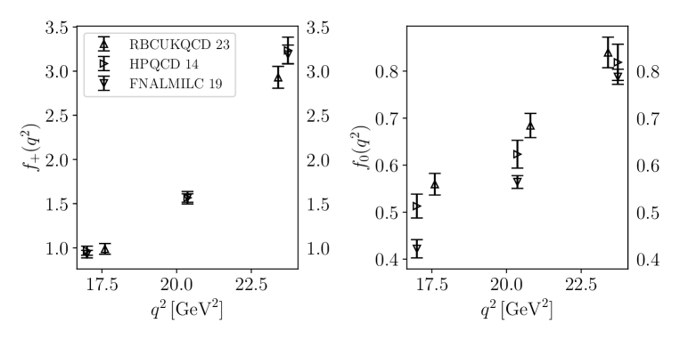
Figure 1: Summary of lattice data used in this study. The data was generated from BCL parameterisations provided in by HPQCD 14 Bouchard:2014ypa and FNAL/MILC 19 Bazavov:2019aom . The values for RBC/UKQCD 23 Flynn:2023nhi are from Tabs. VII and VIII in their paper.

			$f_{+}$			$f_{0}$
	$q^{2}\,[{\rm GeV}^{2}]$		$17.00$	$20.36$	$23.73$	$17.00$	$20.36$	$23.73$
		$f_{+/0}$	0.968(51)	1.567(71)	3.24(15)	0.513(25)	0.623(30)	0.819(38)
$f_{+}$	$17.00$	0.968(51)	1.0000	0.9276	0.5854	0.4293	0.3864	0.3486
	$20.36$	1.567(71)	0.9276	1.0000	0.8047	0.4346	0.4136	0.3645
	$23.73$	3.24(15)	0.5854	0.8047	1.0000	0.4033	0.3707	0.3129
$f_{0}$	$17.00$	0.513(25)	0.4293	0.4346	0.4033	1.0000	0.9646	0.8713
	$20.36$	0.623(30)	0.3864	0.4136	0.3707	0.9646	1.0000	0.9552
	$23.73$	0.819(38)	0.3486	0.3645	0.3129	0.8713	0.9552	1.0000

Table 1: Form factor data from HPQCD 14 Bouchard:2014ypa . The table shows form-factor reference values and errors for given $q^{2}$, and the corresponding the correlation matrix.

			$f_{+}$			$f_{0}$
	$q^{2}\,[{\rm GeV}^{2}]$		$17.00$	$20.36$	$23.73$	$17.00$	$20.36$	$23.73$
		$f_{+/0}$	0.928(43)	1.564(48)	3.19(11)	0.422(19)	0.564(14)	0.788(16)
$f_{+}$	$17.00$	0.928(43)	1.0000	0.8447	0.2180	0.6910	0.5889	0.3707
	$20.36$	1.564(48)	0.8447	1.0000	0.6654	0.4604	0.5864	0.5070
	$23.73$	3.19(11)	0.2180	0.6654	1.0000	0.1310	0.3447	0.3901
$f_{0}$	$17.00$	0.422(19)	0.6910	0.4604	0.1310	1.0000	0.8025	0.3754
	$20.36$	0.564(14)	0.5889	0.5864	0.3447	0.8025	1.0000	0.7727
	$23.73$	0.788(16)	0.3707	0.5070	0.3901	0.3754	0.7727	1.0000

Table 2: Form factor data from FNAL/MILC 19 Bazavov:2019aom . The table shows form-factor reference values and errors for given reference-$q^{2}$ values, and the correlation matrix.

			$f_{+}$		$f_{0}$
	$q^{2}\,[{\rm GeV}^{2}]$		$17.60$	$23.40$	$17.60$	$20.80$	$23.40$
		$f_{+/0}$	0.988(60)	2.93(12)	0.559(23)	0.684(26)	0.840(33)
$f_{+}$	$17.60$	0.988(60)	1.0000	0.8473	0.7322	0.7654	0.7439
	$23.40$	2.93(12)	0.8473	1.0000	0.6544	0.8146	0.8356
$f_{0}$	$17.60$	0.559(23)	0.7322	0.6544	1.0000	0.8816	0.8206
	$20.80$	0.684(26)	0.7654	0.8146	0.8816	1.0000	0.9828
	$23.40$	0.840(33)	0.7439	0.8356	0.8206	0.9828	1.0000

Table 3: Form factor data from RBC/UKQCD 23 Flynn:2023nhi . The table shows form-factor reference values and errors for given $q^{2}$, and the corresponding the correlation matrix.

4.2 Fits to individual data sets

In this section we will apply both the frequentist and our new Bayesian-inference fit strategies individually to the three lattice-data sets. We will first discuss the BGL-fit results and then in Sec. 5 discuss a number of phenomenological predictions.

HPQCD 14 – ${\bf a}_{+}$

$K_{+}$	$K_{0}$	$a_{+,0}$	$a_{+,1}$	$a_{+,2}$	$p$	$\chi^{2}/N_{\rm dof}$	$N_{\rm dof}$
2	2	0.0270(13)	-0.0792(50)	-	0.03	2.93	3
2	3	0.0273(13)	-0.0760(63)	-	0.02	4.06	2
3	2	0.0257(14)	-0.0805(50)	0.068(31)	0.15	1.89	2
3	3	0.0262(14)	-0.0727(64)	0.096(34)	0.97	0.00	1

FNAL/MILC 19 – ${\bf a}_{+}$

$K_{+}$	$K_{0}$	$a_{+,0}$	$a_{+,1}$	$a_{+,2}$	$p$	$\chi^{2}/N_{\rm dof}$	$N_{\rm dof}$
2	2	0.02489(94)	-0.0915(47)	-	0.00	6.52	3
2	3	0.0263(10)	-0.0827(52)	-	0.12	2.12	2
3	2	0.0239(10)	-0.0953(50)	0.044(19)	0.00	7.23	2
3	3	0.0255(11)	-0.0858(57)	0.027(20)	0.12	2.38	1

RBC/UKQCD 23 – ${\bf a}_{+}$

$K_{+}$	$K_{0}$	$a_{+,0}$	$a_{+,1}$	$a_{+,2}$	$p$	$\chi^{2}/N_{\rm dof}$	$N_{\rm dof}$
2	2	0.0293(11)	-0.0871(47)	-	0.00	9.52	2
2	3	0.0249(16)	-0.0999(57)	-	0.04	4.33	1
3	2	0.0245(16)	-0.0798(50)	0.093(21)	0.84	0.04	1

HPQCD 14 – ${\bf a}_{0}$

$K_{+}$	$K_{0}$	$a_{0,0}$	$a_{0,1}$	$a_{0,2}$	$p$	$\chi^{2}/N_{\rm dof}$	$N_{\rm dof}$
2	2	0.0883(44)	-0.250(17)	-	0.03	2.93	3
2	3	0.0880(44)	-0.242(19)	0.053(65)	0.02	4.06	2
3	2	0.0906(45)	-0.240(17)	-	0.15	1.89	2
3	3	0.0908(46)	-0.215(22)	0.138(71)	0.97	0.00	1

FNAL/MILC 19 – ${\bf a}_{0}$

$K_{+}$	$K_{0}$	$a_{0,0}$	$a_{0,1}$	$a_{0,2}$	$p$	$\chi^{2}/N_{\rm dof}$	$N_{\rm dof}$
2	2	0.0775(28)	-0.275(13)	-	0.00	6.52	3
2	3	0.0775(28)	-0.252(15)	0.153(39)	0.12	2.12	2
3	2	0.0774(28)	-0.274(13)	-	0.00	7.23	2
3	3	0.0774(28)	-0.254(15)	0.140(40)	0.12	2.38	1

RBC/UKQCD 23 – ${\bf a}_{0}$

$K_{+}$	$K_{0}$	$a_{0,0}$	$a_{0,1}$	$a_{0,2}$	$p$	$\chi^{2}/N_{\rm dof}$	$N_{\rm dof}$
2	2	0.0981(36)	-0.287(15)	-	0.00	9.52	2
2	3	0.0917(40)	-0.331(19)	-0.210(55)	0.04	4.33	1
3	2	0.0950(37)	-0.262(16)	-	0.84	0.04	1

Table 4: Results for the frequentist BGL fit to HPQCD 14, FNAL/MILC 19 and RBC/UKQCD 23. The tables show the results for BGL coefficients for different orders of the fit.

4.2.1 Results for frequentist fits

Tab. 4 summarises the results of a frequentist analysis for all three data sets, where in each case we performed a simultaneous correlated fit to $f_{+}$ and $f_{0}$, subject to the constraints $f_{+}(0)=f_{0}(0)$ and $N_{\rm dof}\geq 1$. We make the following observations:

• Judging by the $p$-value fits with $(K_{+},K_{0})=(2,2),\,(2,3)$ are excluded by HPQCD 14 and RBC/UKQCD 23, while fits with $K_{+}\geq 3$ and $K_{0}\geq 2$ lead to acceptable fits for all data sets. Note that this is a data-dependent observation since one expects higher-order terms to be important for acceptable fits once results for form factors with higher precision become available.

• For HPQCD 14 we find some variation of the ${\bf a}_{+,1}$ coefficients at the 1$\sigma$ level between $(K_{+},K_{0})=(3,2)$ and (3,3). For ${\bf a}_{0}$ we see a similar variation in $a_{0,1}$, and we obtain only one fit with acceptable $p$-value that is able to determine $a_{0,2}$.

• For FNAL/MILC 19 we obtain acceptable fits only for $(K_{+},K_{0})=(2,3$) and (3,3). We find the coefficients that are common to both truncations to agree within one standard deviation.

• For RBC/UKQCD 23 only fits with $(K_{+},K_{0})=(2,2),\,(2,3)$ and $(3,2)$ are possible. There is essentially only one acceptable fit, the one with $(3,2)$. Consequently no statements about convergence of the fit parameters are possible.

• HPQCD 14 and RBC/UKQCD 23 obtain compatible results, which are however in tension with FNAL/MILC 19 – this is in line with the observation in Fig. 1, that the respective data sets appear to be under tension.

For frequentist fits the constraint $N_{\rm dof}\geq 1$ severely limits the ability to probe the truncation dependence of the fit, and an irreducible systematic error remains. After the above considerations one could choose the results with truncations $(3,3)$ for HPQCD 14 and FNAL/MILC 19, respectively, and $(3,2)$ for RBC/UKQCD 23. Whether higher-order coefficients could still significantly modify these results has to be delegated to a systematic error budget, for which in our opinion no satisfactory procedure exists.

4.2.2 Results for Bayesian inference

HPQCD 14 – ${\bf a}_{+}$

$K_{+}$	$K_{0}$	$a_{+,0}$	$a_{+,1}$	$a_{+,2}$	$a_{+,3}$	$a_{+,4}$	$a_{+,5}$	$a_{+,6}$	$a_{+,7}$	$a_{+,8}$	$a_{+,9}$
2	2	0.0270(12)	-0.0792(49)	-	-	-	-	-	-	-	-
2	3	0.0273(13)	-0.0761(63)	-	-	-	-	-	-	-	-
3	2	0.0257(14)	-0.0805(49)	0.069(30)	-	-	-	-	-	-	-
3	3	0.0261(14)	-0.0728(64)	0.096(34)	-	-	-	-	-	-	-
3	4	0.0261(14)	-0.0728(76)	0.096(39)	-	-	-	-	-	-	-
4	3	0.0261(14)	-0.0729(68)	0.096(35)	0.008(90)	-	-	-	-	-	-
4	4	0.0261(14)	-0.0730(77)	0.091(62)	-0.02(20)	-	-	-	-	-	-
5	5	0.0262(15)	-0.0735(79)	0.084(67)	-0.03(19)	0.03(68)	-	-	-	-	-
6	6	0.0261(14)	-0.0735(79)	0.086(69)	-0.03(19)	-0.00(64)	0.01(65)	-	-	-	-
7	7	0.0262(14)	-0.0732(84)	0.088(69)	-0.02(18)	0.01(65)	0.02(73)	-0.03(70)	-	-	-
8	8	0.0261(14)	-0.0732(80)	0.089(72)	-0.02(18)	-0.00(66)	0.03(86)	-0.04(90)	0.03(73)	-	-
9	9	0.0261(14)	-0.0729(84)	0.095(75)	-0.02(19)	-0.04(68)	0.1(1.0)	-0.1(1.2)	0.1(1.1)	-0.06(79)	-
10	10	0.0261(14)	-0.0726(89)	0.101(79)	-0.01(20)	-0.09(73)	0.2(1.3)	-0.3(1.7)	0.2(1.8)	-0.2(1.4)	0.08(87)

FNAL/MILC 19 – ${\bf a}_{+}$

$K_{+}$	$K_{0}$	$a_{+,0}$	$a_{+,1}$	$a_{+,2}$	$a_{+,3}$	$a_{+,4}$	$a_{+,5}$	$a_{+,6}$	$a_{+,7}$	$a_{+,8}$	$a_{+,9}$
2	2	0.02489(92)	-0.0916(46)	-	-	-	-	-	-	-	-
2	3	0.02626(99)	-0.0827(51)	-	-	-	-	-	-	-	-
3	2	0.0239(10)	-0.0955(49)	0.044(19)	-	-	-	-	-	-	-
3	3	0.0255(11)	-0.0856(56)	0.027(20)	-	-	-	-	-	-	-
3	4	0.0248(12)	-0.0949(80)	0.003(25)	-	-	-	-	-	-	-
4	3	0.0248(12)	-0.0972(92)	-0.026(40)	-0.094(60)	-	-	-	-	-	-
4	4	0.0248(12)	-0.0967(96)	-0.026(64)	-0.09(18)	-	-	-	-	-	-
5	5	0.0248(12)	-0.0968(98)	-0.026(67)	-0.08(18)	0.05(67)	-	-	-	-	-
6	6	0.0249(12)	-0.0964(98)	-0.021(68)	-0.07(17)	0.02(64)	-0.01(67)	-	-	-	-
7	7	0.0248(12)	-0.0961(96)	-0.017(69)	-0.06(17)	0.03(63)	-0.03(73)	0.00(68)	-	-	-
8	8	0.0248(12)	-0.096(10)	-0.012(73)	-0.05(17)	0.02(66)	-0.01(87)	-0.02(89)	0.01(72)	-	-
9	9	0.0249(13)	-0.095(10)	-0.004(73)	-0.03(18)	-0.02(69)	0.0(1.1)	-0.0(1.2)	0.0(1.1)	-0.01(78)	-
10	10	0.0249(12)	-0.094(10)	0.003(78)	-0.01(19)	-0.04(73)	0.1(1.3)	-0.1(1.7)	0.1(1.7)	-0.1(1.4)	0.03(85)

RBC/UKQCD 23 – ${\bf a}_{+}$

$K_{+}$	$K_{0}$	$a_{+,0}$	$a_{+,1}$	$a_{+,2}$	$a_{+,3}$	$a_{+,4}$	$a_{+,5}$	$a_{+,6}$	$a_{+,7}$	$a_{+,8}$	$a_{+,9}$
2	2	0.0293(11)	-0.0871(46)	-	-	-	-	-	-	-	-
2	3	0.0249(16)	-0.0999(57)	-	-	-	-	-	-	-	-
3	2	0.0245(16)	-0.0799(50)	0.093(21)	-	-	-	-	-	-	-
3	3	0.0245(15)	-0.078(12)	0.101(49)	-	-	-	-	-	-	-
3	4	0.0246(16)	-0.078(16)	0.100(70)	-	-	-	-	-	-	-
4	3	0.0246(17)	-0.075(31)	0.102(49)	-0.07(72)	-	-	-	-	-	-
4	4	0.0246(17)	-0.077(32)	0.100(68)	-0.03(70)	-	-	-	-	-	-
5	5	0.0246(17)	-0.074(31)	0.099(70)	-0.08(67)	0.05(70)	-	-	-	-	-
6	6	0.0247(16)	-0.073(32)	0.101(69)	-0.10(69)	0.09(74)	-0.05(71)	-	-	-	-
7	7	0.0247(17)	-0.071(33)	0.107(70)	-0.11(72)	0.08(89)	-0.04(89)	0.03(73)	-	-	-
8	8	0.0248(17)	-0.068(35)	0.102(74)	-0.18(77)	0.2(1.1)	-0.2(1.3)	0.1(1.2)	-0.06(82)	-	-
9	9	0.0248(18)	-0.068(38)	0.107(85)	-0.16(82)	0.2(1.4)	-0.2(1.9)	0.1(1.9)	-0.1(1.5)	0.03(89)	-
10	10	0.0247(18)	-0.067(43)	0.112(95)	-0.15(90)	0.2(1.8)	-0.2(2.6)	0.1(2.9)	-0.1(2.7)	-0.0(1.9)	0.02(98)

Table 5: Results for the individual Bayesian-inference BGL fits to HPQCD 14, FNAL/MILC 19 and RBC/UKQCD 23, respectively. The tables show the results for BGL coefficients ${\bf a_{+}}$ for different orders of the fit.

HPQCD 14 – ${\bf a}_{0}$

$K_{+}$	$K_{0}$	$a_{0,0}$	$a_{0,1}$	$a_{0,2}$	$a_{0,3}$	$a_{0,4}$	$a_{0,5}$	$a_{0,6}$	$a_{0,7}$	$a_{0,8}$	$a_{0,9}$
2	2	0.0883(44)	-0.250(17)	-	-	-	-	-	-	-	-
2	3	0.0880(44)	-0.243(19)	0.052(65)	-	-	-	-	-	-	-
3	2	0.0907(46)	-0.240(17)	-	-	-	-	-	-	-	-
3	3	0.0906(44)	-0.215(22)	0.137(73)	-	-	-	-	-	-	-
3	4	0.0907(47)	-0.215(22)	0.14(11)	-0.01(31)	-	-	-	-	-	-
4	3	0.0907(45)	-0.214(22)	0.139(72)	-	-	-	-	-	-	-
4	4	0.0907(46)	-0.215(25)	0.12(19)	-0.08(60)	-	-	-	-	-	-
5	5	0.0909(46)	-0.218(25)	0.10(19)	-0.12(55)	0.04(63)	-	-	-	-	-
6	6	0.0907(45)	-0.217(25)	0.10(19)	-0.11(53)	0.06(66)	-0.02(66)	-	-	-	-
7	7	0.0907(46)	-0.217(26)	0.11(20)	-0.08(51)	0.03(73)	0.03(81)	-0.04(70)	-	-	-
8	8	0.0908(46)	-0.217(25)	0.11(20)	-0.08(50)	-0.01(84)	0.1(1.0)	-0.09(96)	0.08(74)	-	-
9	9	0.0907(46)	-0.215(25)	0.13(22)	-0.05(50)	-0.06(95)	0.2(1.4)	-0.2(1.5)	0.1(1.2)	-0.05(82)	-
10	10	0.0907(46)	-0.214(27)	0.15(24)	-0.03(49)	-0.2(1.1)	0.4(1.8)	-0.5(2.2)	0.4(2.1)	-0.3(1.6)	0.13(90)

FNAL/MILC 19 – ${\bf a}_{0}$

$K_{+}$	$K_{0}$	$a_{0,0}$	$a_{0,1}$	$a_{0,2}$	$a_{0,3}$	$a_{0,4}$	$a_{0,5}$	$a_{0,6}$	$a_{0,7}$	$a_{0,8}$	$a_{0,9}$
2	2	0.0775(27)	-0.275(13)	-	-	-	-	-	-	-	-
2	3	0.0775(27)	-0.253(15)	0.153(39)	-	-	-	-	-	-	-
3	2	0.0773(28)	-0.274(13)	-	-	-	-	-	-	-	-
3	3	0.0775(28)	-0.253(15)	0.141(40)	-	-	-	-	-	-	-
3	4	0.0735(36)	-0.297(31)	0.088(51)	0.32(20)	-	-	-	-	-	-
4	3	0.0734(38)	-0.305(36)	-0.01(10)	-	-	-	-	-	-	-
4	4	0.0736(38)	-0.304(37)	-0.01(20)	-0.00(61)	-	-	-	-	-	-
5	5	0.0735(38)	-0.303(36)	-0.00(20)	0.01(55)	-0.05(62)	-	-	-	-	-
6	6	0.0736(37)	-0.301(36)	0.01(20)	0.04(52)	-0.07(64)	0.07(63)	-	-	-	-
7	7	0.0735(38)	-0.300(36)	0.03(20)	0.07(51)	-0.18(73)	0.19(78)	-0.14(69)	-	-	-
8	8	0.0737(38)	-0.298(36)	0.05(21)	0.09(51)	-0.25(85)	0.3(1.1)	-0.28(99)	0.15(74)	-	-
9	9	0.0736(40)	-0.296(36)	0.08(22)	0.15(50)	-0.41(97)	0.6(1.4)	-0.6(1.5)	0.4(1.2)	-0.19(80)	-
10	10	0.0738(36)	-0.292(35)	0.11(24)	0.17(49)	-0.6(1.1)	0.9(1.8)	-1.0(2.2)	0.8(2.1)	-0.5(1.6)	0.18(90)

RBC/UKQCD 23 – ${\bf a}_{0}$

$K_{+}$	$K_{0}$	$a_{0,0}$	$a_{0,1}$	$a_{0,2}$	$a_{0,3}$	$a_{0,4}$	$a_{0,5}$	$a_{0,6}$	$a_{0,7}$	$a_{0,8}$	$a_{0,9}$
2	2	0.0981(36)	-0.286(14)	-	-	-	-	-	-	-	-
2	3	0.0917(39)	-0.331(19)	-0.211(53)	-	-	-	-	-	-	-
3	2	0.0950(37)	-0.263(15)	-	-	-	-	-	-	-	-
3	3	0.0953(43)	-0.254(41)	0.02(13)	-	-	-	-	-	-	-
3	4	0.0955(44)	-0.254(42)	0.02(22)	-0.02(60)	-	-	-	-	-	-
4	3	0.0954(43)	-0.254(40)	0.03(12)	-	-	-	-	-	-	-
4	4	0.0953(42)	-0.254(42)	0.02(21)	-0.02(60)	-	-	-	-	-	-
5	5	0.0954(44)	-0.254(41)	0.02(21)	-0.01(55)	-0.00(62)	-	-	-	-	-
6	6	0.0957(42)	-0.251(41)	0.04(21)	-0.01(52)	-0.06(65)	0.07(65)	-	-	-	-
7	7	0.0955(44)	-0.250(40)	0.06(20)	0.05(50)	-0.13(72)	0.17(79)	-0.12(69)	-	-	-
8	8	0.0954(43)	-0.250(41)	0.06(22)	0.06(50)	-0.18(84)	0.2(1.0)	-0.21(99)	0.10(74)	-	-
9	9	0.0956(44)	-0.247(41)	0.08(23)	0.06(50)	-0.27(96)	0.4(1.4)	-0.4(1.5)	0.3(1.2)	-0.15(80)	-
10	10	0.0956(42)	-0.245(42)	0.11(24)	0.11(49)	-0.4(1.1)	0.7(1.8)	-0.8(2.2)	0.7(2.1)	-0.4(1.5)	0.16(87)

Table 6: Results for the individual Bayesian-inference BGL fits to HPQCD 14, FNAL/MILC 19 and RBC/UKQCD 23, respectively. The tables show the results for BGL coefficients ${\bf a_{0}}$ for different orders of the fit.

Here we repeat the same fits as in the previous section but now using the new Bayesian-inference approach, which allows us to analyse the data with higher truncation $(K_{+},K_{0})$ than possible in the frequentist case. Tabs. 5 and 6 show the results for Bayesian inference, and in Fig. 2 we exemplarily show the result of the Bayesian-inference fit to the HPQCD 14 data. We make the following observations:

• Frequentist fits and Bayesian inference, where possible at the same $(K_{+},K_{0}$) agree. This is the expected behaviour: The fit results for the $B_{s}\to K\ell\nu$ decay considered here do not saturate the unitarity constraint Eq. (12). In this situation the maximum and width of the probability distribution Eq. (30) in Bayesian inference are described by the results obtained for central values ${\bf a}$ and covariance $C_{\bf a}$ in the frequentist fit, as given in Eq. (22) and (23).

• The power of Bayesian inference lies in the fact that the order of the $z$ expansion can be extended beyond the frequentist constraint $N_{\rm dof}\geq 1$: The data in Tabs. 5 and 6 shows that the central values for the BGL coefficients converge to stable central values. The unitarity constraint in Eq. (12) efficiently regulates the fluctuations of higher-order coefficients. By making use of unitarity and analyticity the hard-to-estimate truncation errors in the frequentist fit have been replaced by well-motivated and model-independent statistical noise originating from the undetermined higher-order coefficients.

• Note that in particular the samples of higher-order coefficients may not necessarily follow a normal distribution, in particular if they are determined mainly through the unitarity constraint. The errors given in the data tables have to be interpreted with this in mind. It may in this context also at first be surprising, that some higher-order coefficients in the tables have central values, which apparently saturate the unitarity constraint. Similarly, some coefficients have at first sight rather large ‘1$\sigma$’ errors, which don’t appear consistent with the unitarity constraint. However, such fluctuations are allowed and compatible with the modified unitarity constraint in Eq. (12). We check in our algorithm that this unitarity constraint is fulfilled at each step of the analysis.

• The maximum truncation shown, $(K_{+},K_{0})=(10,10)$ is only for demonstration purposes – we see no significant changes in the fit coefficients and errors for $(K_{+},K_{0})\geq(5,5)$ and therefore choose this truncation for the main results of our study.

Bayesian inference regulated by unitarity and analyticity proves to be a powerful tool for truncation-independent fits to form-factor data.

4.2.3 Combined Bayesian and frequentist analysis

The Bayesian-inference framework makes no statements about the quality of the BGL fit for a given truncation. Its power lies in its ability to fit the BGL ansatz without truncation error. The frequentist fit on the other hand only provides meaningful results for $N_{\rm dof}\geq 1$, i.e. for a finite truncation. For this finite truncation, however, quality measures like the $p$-value do make statements about how well data and fit function are compatible. It is therefore always advisable to consider both for a comprehensive data analysis. Consider the case where a wrong assumption was made in the fit function, or where the input data is erroneous – apart from a visual inspection of a Bayesian-inference fit clearly indicating that something is wrong, only the frequentist fit provides a quantitative measure for the quality of the fit that could indicate a problem.

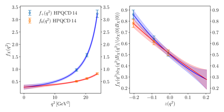
Figure 2: Illustration of the Bayesian-inference fit to the HPQCD-14 data Bouchard:2014ypa with $(K_{+},K_{0})=(5,5)$. Left: plot of the form factor vs. the squared momentum transfer; right: plot of the form factor after removing Blaschke and outer function, normalised such that the kinematical constraint $f_{0}(0)=f_{+}(0)$ becomes apparent.

4.3 Combined fits

It is straight forward to combine results from different sources into one global Bayesian-inference analysis. Essentially, this amounts to extending the data vector ${\bf f}$ and covariance $C_{\bf f}$ by the additional data sets. Correlations between data set can be included by adding the corresponding entries to the off-diagonal blocks of the enlarged covariance matrix.

4.3.1 Combined fits to lattice data

We combine the results for HPQCD 14, FNAL/MILC 19 and RBC/UKQCD 23 in Tab. 1-3, assuming the results and errors from these three data sources to be independent. We find that the FNAL/MILC 19 data on the one hand and the HPQCD 14 and RBC/UKQCD 23 on the other are incompatible, as indicated by visual inspection of Fig. 1, and by unacceptably small $p$-values of such a fit as summarised in Tab. 5.4 in App. F.2. We note that a Bayesian-inference analysis would nevertheless be possible. This just underlines the importance of making best use of the complementary information one gains from frequentist and Bayesian fitting, respectively.

We proceed considering only the combined fit over the data sets by HPQCD 14 and RBC/UKQCD 23. The results for the frequentist and Bayesian BGL fits are presented in Tabs. 7 and 8, respectively.

$K_{+}$	$K_{0}$	$a_{+,0}$	$a_{+,1}$	$a_{+,2}$	$a_{+,3}$	$a_{+,4}$	$p$	$\chi^{2}/N_{\rm dof}$	$N_{\rm dof}$
2	2	0.02805(81)	-0.0822(33)	-	-	-	0.00	4.02	8
2	3	0.0266(10)	-0.0881(40)	-	-	-	0.00	3.69	7
3	2	0.0250(10)	-0.0794(34)	0.083(16)	-	-	0.47	0.95	7
3	3	0.0253(10)	-0.0731(52)	0.110(24)	-	-	0.67	0.67	6
3	4	0.0253(11)	-0.0742(68)	0.105(32)	-	-	0.56	0.79	5
4	3	0.0253(11)	-0.0738(58)	0.111(24)	0.024(89)	-	0.56	0.79	5
4	4	0.0257(13)	-0.038(54)	0.61(74)	1.7(2.5)	-	0.48	0.87	4
5	5	0.0261(14)	-0.002(77)	1.2(1.1)	5.3(6.3)	6.7(18.1)	0.23	1.46	2

$K_{+}$	$K_{0}$	$a_{0,0}$	$a_{0,1}$	$a_{0,2}$	$a_{0,3}$	$a_{0,4}$	$p$	$\chi^{2}/N_{\rm dof}$	$N_{\rm dof}$
2	2	0.0938(27)	-0.270(11)	-	-	-	0.00	4.02	8
2	3	0.0926(28)	-0.289(13)	-0.098(39)	-	-	0.00	3.69	7
3	2	0.0942(27)	-0.256(11)	-	-	-	0.47	0.95	7
3	3	0.0955(29)	-0.234(17)	0.091(56)	-	-	0.67	0.67	6
3	4	0.0955(29)	-0.235(18)	0.07(10)	-0.08(30)	-	0.56	0.79	5
4	3	0.0956(29)	-0.234(18)	0.093(57)	-	-	0.56	0.79	5
4	4	0.0968(34)	-0.11(19)	1.8(2.6)	5.6(8.5)	-	0.48	0.87	4
5	5	0.0967(35)	-0.07(22)	3.2(3.5)	19.7(21.6)	40.7(54.6)	0.23	1.46	2

Table 7: Results for the frequentist BGL fit to HPQCD 14 and RBC/UKQCD 23. The tables show the results for BGL coefficients for different orders of the fit.

$K_{+}$	$K_{0}$	$a_{+,0}$	$a_{+,1}$	$a_{+,2}$	$a_{+,3}$	$a_{+,4}$	$a_{+,5}$	$a_{+,6}$	$a_{+,7}$	$a_{+,8}$	$a_{+,9}$
2	2	0.02805(80)	-0.0821(33)	-	-	-	-	-	-	-	-
2	3	0.02659(99)	-0.0881(39)	-	-	-	-	-	-	-	-
3	2	0.0250(10)	-0.0793(33)	0.083(16)	-	-	-	-	-	-	-
3	3	0.0253(10)	-0.0733(50)	0.110(24)	-	-	-	-	-	-	-
3	4	0.0252(11)	-0.0743(68)	0.105(32)	-	-	-	-	-	-	-
4	3	0.0253(10)	-0.0740(58)	0.112(24)	0.028(89)	-	-	-	-	-	-
4	4	0.0253(11)	-0.0738(66)	0.110(58)	0.02(20)	-	-	-	-	-	-
5	5	0.0253(11)	-0.0738(74)	0.111(64)	0.02(19)	-0.04(68)	-	-	-	-	-
6	6	0.0253(11)	-0.0739(74)	0.107(61)	0.01(19)	-0.01(63)	0.01(66)	-	-	-	-
7	7	0.0253(10)	-0.0734(74)	0.113(64)	0.01(18)	-0.06(64)	0.05(72)	-0.07(69)	-	-	-
8	8	0.0252(11)	-0.0732(78)	0.116(66)	0.01(19)	-0.09(65)	0.12(84)	-0.12(86)	0.10(72)	-	-
9	9	0.0253(10)	-0.0727(75)	0.121(69)	0.01(19)	-0.12(69)	0.2(1.1)	-0.3(1.2)	0.2(1.1)	-0.10(78)	-
10	10	0.0253(11)	-0.0720(85)	0.127(74)	0.00(20)	-0.20(75)	0.4(1.3)	-0.5(1.7)	0.5(1.8)	-0.3(1.4)	0.14(86)

$K_{+}$	$K_{0}$	$a_{0,0}$	$a_{0,1}$	$a_{0,2}$	$a_{0,3}$	$a_{0,4}$	$a_{0,5}$	$a_{0,6}$	$a_{0,7}$	$a_{0,8}$	$a_{0,9}$
2	2	0.0938(27)	-0.269(10)	-	-	-	-	-	-	-	-
2	3	0.0927(28)	-0.289(13)	-0.097(38)	-	-	-	-	-	-	-
3	2	0.0942(27)	-0.256(11)	-	-	-	-	-	-	-	-
3	3	0.0955(28)	-0.235(17)	0.090(55)	-	-	-	-	-	-	-
3	4	0.0954(29)	-0.235(18)	0.07(10)	-0.07(31)	-	-	-	-	-	-
4	3	0.0956(29)	-0.234(18)	0.093(57)	-	-	-	-	-	-	-
4	4	0.0955(29)	-0.234(21)	0.09(19)	-0.02(62)	-	-	-	-	-	-
5	5	0.0956(28)	-0.234(22)	0.09(19)	-0.03(55)	-0.01(64)	-	-	-	-	-
6	6	0.0955(28)	-0.234(22)	0.08(19)	-0.05(51)	0.00(66)	0.03(64)	-	-	-	-
7	7	0.0956(28)	-0.233(22)	0.09(19)	-0.02(50)	-0.06(72)	0.09(79)	-0.07(69)	-	-	-
8	8	0.0955(29)	-0.233(23)	0.10(21)	0.00(50)	-0.09(82)	0.2(1.0)	-0.16(98)	0.11(71)	-	-
9	9	0.0956(29)	-0.231(23)	0.12(22)	0.02(49)	-0.18(98)	0.3(1.4)	-0.3(1.5)	0.2(1.2)	-0.12(79)	-
10	10	0.0956(29)	-0.230(25)	0.13(23)	0.02(48)	-0.3(1.1)	0.5(1.8)	-0.5(2.2)	0.5(2.1)	-0.3(1.6)	0.14(88)

Table 8: Results for the Bayesian-inference BGL fit to HPQCD 14 and RBC/UKQCD 23. The tables show the results for BGL coefficients for different orders of the fit.

Fig. 3 shows the result of the combined Bayesian-inference fit to the RBC/UKQCD 23 and the HPQCD 14 data.

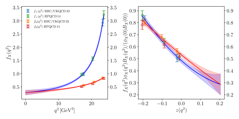
Figure 3: Illustration of the joint Bayesian-inference fit to the HPQCD 14 Bouchard:2014ypa and RBC/UKQCD 23 Flynn:2023nhi data sets with $(K_{+},K_{0})=(5,5)$. Left: plot of the form factor vs. the squared momentum transfer; right: plot of the form factor after removing Blaschke and outer function, normalised such that the kinematical constraint $f_{0}(0)=f_{+}(0)$ becomes apparent.

A look at both tables clarifies that the fit-function is capable of describing the joint data set for $(K_{+},K_{0})\geq(3,2)$ with an acceptable $p$-value but central values and errors for the higher-order coefficients still vary as the values $(K_{+},K_{0})$ are further increased. While the higher-order coefficients fluctuate wildly due to the lack of unitarity constraint in the frequentist ansatz, the results of the Bayesian-inference remain stable when increasing $(K_{+},K_{0})$. The higher-order coefficients remain well controlled.

4.3.2 Combined fits to lattice and sum-rule data

Repeating the fits of the previous section after including the sum-rule result Khodjamirian 17 Khodjamirian:2017fxg leads to the results in Fig. 4 (numerical results can be found in App. F.3 in Tabs. 5.4 and 5.4). While the frequentist fit achieves good $p$-values starting with $(K_{+},K_{0})=(3,3)$, the results of Bayesian inference converge towards stable central values and errors starting with $(K_{+},K_{0})=(4,4)$. Comparing Figs. 3 and 4, highlights the importance that SM predictions at lower $q^{2}$ values can have in stabilising the overall parameterisation of the form factor. This is then also reflected in the smaller error of the respective BGL expansion coefficients listed in Tabs. 8 and 5.4.

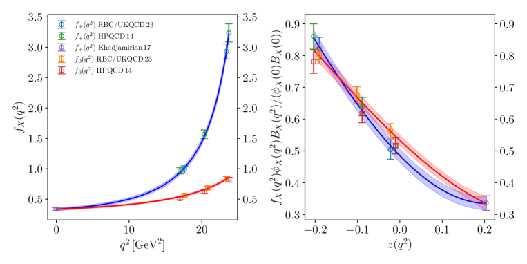
Figure 4: Illustration of the joint Bayesian-inference fit to the HPQCD-14 Bouchard:2014ypa , RBC/UKQCD 23 Flynn:2023nhi and Khodjamirian 17 data sets with $(K_{+},K_{0})=(5,5)$. Left: plot of the form factor vs. the squared momentum transfer; right: plot of the form factor after removing Blaschke and outer function, normalised such that the kinematical constraint $f_{0}(0)=f_{+}(0)$ becomes apparent.

4.4 Comparison with dispersive-matrix method

In this section we compare our results to the dispersive-matrix method Lellouch:1995yv , which has recently received renewed attention in Ref. DiCarlo:2021dzg , and which has been applied to exclusive semileptonic $B_{s}\to K\ell\nu$ decay in Ref. Martinelli:2022tte . Fig. 5 shows the comparison of both methods for the fit to the data set RBC/UKQCD 23. The results for the dispersive-matrix method were obtained with our own implementation of the algorithm proposed in Ref. DiCarlo:2021dzg . We find central values and error bands in excellent agreement.

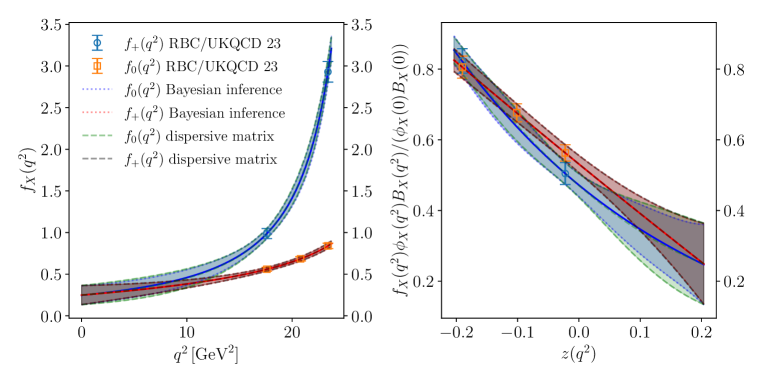
Figure 5: Comparison of Bayesian inference with the dispersive-matrix method for the form factors of exclusive semileptonic $B_{s}\to K\ell\nu$ decay.

While the dispersive-matrix computes a distribution of results for every value of the momentum transfer $q^{2}$, Bayesian inference predicts the parameters of the BGL expansion and their correlations. Besides the conceptual simplicity of the Bayesian-inference fitting strategy, the results for Bayesian inference are hence more convenient for use in further processing, e.g. for making predictions for phenomenology as discussed in the next section.

5 Phenomenological analysis

Having parameterised the form factors $f_{+}(q^{2})$ and $f_{0}(q^{2})$ over the full kinematically allowed phase space $0\leq q^{2}\leq q^{2}_{\rm max}$, various phenomenologically relevant quantities can be computed. In the following we provide determinations of the CKM matrix element $|V_{ub}|$, two versions of the $R$-ratio (the traditional one and an improved version which has been advocated in Ref. Flynn:2023nhi ) and the differential decay rate. Additionally, results and discussion of the forward-backward and polarisation asymmetries can be found in App. E. Here we concentrate mainly on results for combined fits over data sets. The results we would obtain from fits to individual data sets are summarised in tables in App. F.1.

5.1 Determination of $|V_{ub}|$

By combining experimental measurements of $d\Gamma(B_{s}\to K\ell\nu)/dq^{2}$ with theoretical predictions for the form factors $f_{0}$ and $f_{+}$ the CKM matrix element $|V_{ub}|$ can be determined using Eq. (1). Currently, the only available measurements have been performed by LHCb who provide the ratio of branching fractions $R_{BF}$ LHCb:2020ist ,

$$R_{\rm BF}=\frac{\mathcal{B}(B_{s}^{0}\to K^{-}\mu^{+}\nu_{\mu})}{\mathcal{B}(B_{s}^{0}\to D_{s}^{-}\mu^{+}\nu_{\mu})}\,.$$ (34)

These values are given for two integrated $q^{2}$ bins, which we will refer to as ‘low’ and ‘high’,

$$q^{2}\leq 7\,\mathrm{Ge\kern-1.00006ptV}^{2} R^{\rm low}_{BF}=1.66(80)(86)\times 10^{-3}\,,$$:

$$q^{2}\geq 7\,\mathrm{Ge\kern-1.00006ptV}^{2} R^{\rm high}_{BF}=3.25(21)(^{+18}_{-19})\times 10^{-3}\,.$$: (35)

Using the life time of the $B_{s}^{0}$ meson $\tau_{B_{s}^{0}}=1.520(5)\,\mathrm{ps}$ HFLAV:2022pwe ; ParticleDataGroup:2022pth and the branching ratio LHCb:2020cyw

$$\mathcal{B}(B_{s}^{0}\to D_{s}^{-}\mu^{+}\nu_{\mu})=2.49(12)(21)\times 10^{-2}\,,$$ (36)

this can be used to determine $|V_{ub}|$ from

$$|V_{ub}|=\sqrt{\frac{R^{\rm bin}_{BF}\,\mathcal{B}(B_{s}^{0}\to D_{s}^{-}\mu^{+}\nu_{\mu})}{\tau_{B_{s}^{0}}\,\Gamma^{\rm bin}_{0}(B_{s}\to K\ell\nu)}}\,,$$ (37)

where we defined the reduced decay rate $\Gamma^{\rm bin}_{0}=\Gamma^{\rm bin}/|V_{ub}|^{2}$. Since we have obtained the BGL parameterisation of the form factors, $\Gamma^{\rm bin}_{0}$ can be computed by numerically integrating the right-hand side of Eq. (1) over the appropriate $q^{2}$ bin. After symmetrising the errors on the input data, we generate multivariate distributions for the aforementioned experimental inputs, assuming the systematic uncertainties of the branching fractions $R_{BF}$ and the branching ratio $\mathcal{B}$ to be 100% correlated and all other uncertainties to be uncorrelated (cf. Ref. Martinelli:2022tte ). The form factors $f_{0}$ and $f_{+}$ are constructed from the samples for the BGL coefficients that we have found from our algorithm. Combining these distributions provides a fully correlated analysis framework to determine $|V_{ub}|$ from either bin as well as from a weighted average. Numerical values of our results are presented in Tab. 9.

$K_{+}$	$K_{0}$	$f(q^{2}=0)$	$R_{B_{s}\to K}^{\rm impr}$	$R_{B_{s}\to K}$	$\frac{\Gamma^{\tau}}{|V_{ub}|^{2}}\,[\frac{1}{\rm ps}]$	$\frac{\Gamma^{\mu}}{|V_{ub}|^{2}}\,[\frac{1}{\rm ps}]$	$V^{\rm low}_{\rm CKM}$	$V^{\rm high}_{\rm CKM}$	$V^{\rm full}_{\rm CKM}$
2	2	0.217(16)	1.544(15)	0.735(15)	4.94(31)	6.72(51)	0.00365(35)	0.00338(30)	0.00349(31)
2	3	0.166(25)	1.587(26)	0.809(37)	4.36(36)	5.41(65)	0.00449(64)	0.00365(36)	0.00386(41)
3	2	0.234(16)	1.684(38)	0.758(19)	4.41(31)	5.83(51)	0.00367(35)	0.00374(34)	0.00370(33)
3	3	0.286(36)	1.682(36)	0.700(37)	4.80(40)	6.89(87)	0.00319(41)	0.00359(34)	0.00343(35)
3	4	0.277(53)	1.688(42)	0.715(64)	4.73(46)	6.7(1.2)	0.00333(60)	0.00364(36)	0.00356(40)
4	3	0.288(37)	1.689(42)	0.701(39)	4.79(41)	6.87(90)	0.00319(42)	0.00362(35)	0.00344(35)
4	4	0.286(93)	1.687(41)	0.709(98)	4.80(54)	7.0(1.6)	0.00335(88)	0.00362(37)	0.00358(41)
5	5	0.286(87)	1.686(44)	0.709(94)	4.81(54)	7.0(1.6)	0.00332(86)	0.00360(36)	0.00356(41)
6	6	0.282(85)	1.686(45)	0.713(93)	4.78(53)	6.9(1.6)	0.00336(85)	0.00361(37)	0.00357(41)
7	7	0.288(85)	1.686(44)	0.706(90)	4.81(54)	7.0(1.6)	0.00330(80)	0.00361(36)	0.00355(40)
8	8	0.290(90)	1.686(44)	0.704(96)	4.82(57)	7.1(1.7)	0.00330(89)	0.00361(38)	0.00356(42)
9	9	0.297(90)	1.685(43)	0.697(95)	4.87(56)	7.2(1.7)	0.00324(87)	0.00359(37)	0.00353(42)
10	10	0.300(93)	1.685(44)	0.694(98)	4.89(59)	7.3(1.8)	0.00322(86)	0.00357(37)	0.00352(42)

$K_{+}$	$K_{0}$	$I[\mathcal{A}_{\rm FB}^{\tau}]\,[\frac{1}{\rm ps}]$	$I[\mathcal{A}_{\rm FB}^{\mu}]\,[\frac{1}{\rm ps}]$	$\mathcal{\bar{A}}_{\rm FB}^{\tau}$	$\mathcal{\bar{A}}_{\rm FB}^{\mu}$	$I[\mathcal{A}_{\rm pol}^{\tau}]\,[\frac{1}{\rm ps}]$	$I[\mathcal{A}_{\rm pol}^{\mu}]\,[\frac{1}{\rm ps}]$	$\mathcal{\bar{A}}_{\rm pol}^{\tau}$	$\mathcal{\bar{A}}_{\rm pol}^{\mu}$
2	2	1.345(87)	0.0302(34)	0.2724(18)	0.00448(21)	0.732(72)	6.64(50)	0.148(12)	0.98749(57)
2	3	1.18(10)	0.0212(42)	0.2715(18)	0.00388(33)	0.53(10)	5.35(64)	0.121(17)	0.98887(80)
3	2	1.243(88)	0.0322(36)	0.2817(22)	0.00551(31)	0.23(11)	5.74(51)	0.052(24)	0.98422(93)
3	3	1.37(12)	0.0439(88)	0.2855(32)	0.00632(59)	0.24(12)	6.76(85)	0.050(23)	0.9821(16)
3	4	1.35(14)	0.042(12)	0.2851(37)	0.00618(82)	0.23(13)	6.6(1.1)	0.047(25)	0.9825(21)
4	3	1.37(12)	0.0443(91)	0.2858(33)	0.00640(63)	0.22(13)	6.75(88)	0.046(26)	0.9819(17)
4	4	1.37(17)	0.046(21)	0.2856(58)	0.0063(16)	0.23(13)	6.8(1.6)	0.047(26)	0.9821(41)
5	5	1.38(17)	0.046(20)	0.2855(56)	0.0063(15)	0.23(14)	6.9(1.5)	0.048(27)	0.9822(39)
6	6	1.37(17)	0.045(19)	0.2852(56)	0.0062(15)	0.23(14)	6.8(1.5)	0.048(28)	0.9823(38)
7	7	1.38(17)	0.046(20)	0.2856(55)	0.0063(14)	0.23(14)	6.9(1.6)	0.048(27)	0.9821(37)
8	8	1.38(19)	0.047(21)	0.2858(59)	0.0064(15)	0.23(14)	6.9(1.6)	0.048(27)	0.9820(39)
9	9	1.40(18)	0.049(21)	0.2862(59)	0.0065(15)	0.23(13)	7.1(1.6)	0.047(27)	0.9818(39)
10	10	1.40(19)	0.050(23)	0.2864(61)	0.0065(15)	0.23(14)	7.2(1.8)	0.048(27)	0.9817(40)

Table 9: Summary of results based on combined fit to HPQCD 14 Bouchard:2014ypa and RBC/UKQCD 23 Flynn:2023nhi . Definitions for the asymmetries $\mathcal{A}$ can be found in App. E.

For the combined fit to HPQCD 14 and RBC/UKQCD 23 we find the results to be stable for $(K_{+},K_{0})\geq(5,5)$ and we choose this truncation for our main result

$$|V_{ub}|= 3.56(41)\times 10^{-3}\,\,\textrm{\cite[cite]{\@@bibref{Authors Phrase1YearPhrase2}{Bouchard:2014ypa,Flynn:2023nhi}{\@@citephrase{(}}{\@@citephrase{)}}}}.$$ (38)

As we will see shortly, also other observables that we computed have stable central values and errors when further increasing the truncation. We make the same choice $(K_{+},K_{0})=(5,5)$ for the combined fit to lattice and sum-rule data HPQCD 14 and RBC/UKQCD 23 and Khodjamirian 17,

$$|V_{ub}|= 3.13(28)\times 10^{-3}\,\,\textrm{\cite[cite]{\@@bibref{Authors Phrase1YearPhrase2}{Bouchard:2014ypa,Flynn:2023nhi,Khodjamirian:2017fxg}{\@@citephrase{(}}{\@@citephrase{)}}}}.$$ (39)

In both cases, the error on $|V_{ub}|$ is currently dominated by the experimental uncertainty (we ran the fit again assuming vanishing experimental uncertainties and obtained $|V_{ub}|=3.67(17)\times 10^{-3}$ and $|V_{ub}|=3.23(14)\times 10^{-3}$, respectively). We note that while the results for $|V_{ub}|$ obtained for the ‘low’ and ‘high’ bins agree for the analysis with HPQCD 14 and RBC/UKQCD 23 (cf. Tab. 9), they are at tension in the analysis that also includes the sum-rule result Khodjamirian 17 (cf. Tab. 17), where $|V_{ub}^{\rm low}|=2.84(27)$ and $|V_{ub}^{\rm high}|=3.54(33)$. For comparison we quote the world averages for exclusive and inclusive determinations of $|V_{ub}|$

$$|V_{ub}|_{\rm exclusive}^{\rm FLAG\,21}\times 10^{-3}= \,3.74(17)\,\textrm{ \cite[cite]{\@@bibref{Authors Phrase1YearPhrase2}{Lattice:2015tia,Flynn:2015mha,delAmoSanchez:2010af,Lees:2012vv,Ha:2010rf,Sibidanov:2013rkk,FlavourLatticeAveragingGroupFLAG:2021npn}{\@@citephrase{(}}{\@@citephrase{)}}}}\,,$$ (40)

$$|V_{ub}|_{\rm inclusive}\times 10^{-3}= \,4.13(26)\,\textrm{\cite[cite]{\@@bibref{Authors Phrase1YearPhrase2}{ParticleDataGroup:2022pth, HFLAV:2022pwe, Gambino:2007rp, Lange:2005yw, Andersen:2005mj}{\@@citephrase{(}}{\@@citephrase{)}}}}\,\,.$$ (41)

5.2 Differential decay width

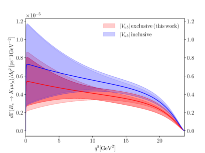
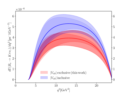
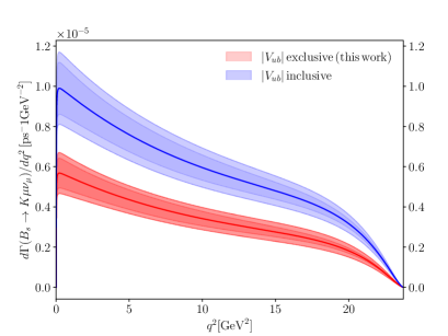
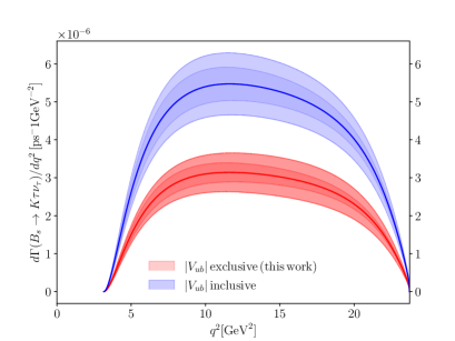
Figure 6: The differential decay width $d\Gamma/dq^{2}$ for $B_{s}\to K\mu\nu_{\mu}$ (left) and $B_{s}\to K\tau\nu_{\tau}$ (right). The top row shows results from the fit to HPQCD 14 and RBQ/UKQCD 23, while the lower panel shows the result where the fit also includes the sum-rule result Khodjamirian 17. The values for $|V_{ub}|$ are taken from Eq. (41), (38) (top) and (39) (bottom). The darker (lighter) shading indicates the error without (with) the contribution from the error on $|V_{ub}|$.

From the analysis of lattice and sum-rule data we can make SM predictions for the shape of the differential decay width $d\Gamma/dq^{2}$. In Fig. 6 we illustrate this, assuming our result for $|V_{ub}|$ from the lattice and lattice+sum rules analyses in Eq. (38) and (39), and the results from the inclusive decay analysis in Eqs. (41). The predicted shapes of the inclusive and exclusive differential decay rates are visibly different. In particular, after including the sum-rule result, the shapes can be clearly and statistically significantly distinguished. Such detailed studies of decay-rate shapes can shed light on the tension between inclusive and exclusive CKM determinations.

5.3 $R$ ratios

Lepton flavour universality (LFU), i.e. the identical coupling of leptons to gauge bosons, is an accidental symmetry of the SM. Testing LFU therefore provides crucial tests of the SM. One way to perform such tests is by comparing semileptonic decays with different leptons in the final state. Due to their different masses, the shapes of the differential decay rates and (partial) integrals thereof will differ. Of particular interest are ratios which are independent of the relevant CKM matrix elements (in our case $|V_{ub}|$) since this eliminates sources of uncertainty. One such observable is the traditional $R$-ratio, defined by

$$R_{B_{s}\to K}=\frac{\int_{m_{\tau}^{2}}^{q^{2}_{\text{max}}}dq^{2}\,\frac{d\Gamma(B_{s}\to K\tau\nu_{\tau})}{dq^{2}}}{\int_{m_{\ell}^{2}}^{q^{2}_{\text{max}}}dq^{2}\,\frac{d\Gamma(B_{s}\to K\ell\nu_{\ell})}{dq^{2}}}\,.$$ (42)

Here $\ell$ denotes the $e$ or $\mu$, whereas the numerator only contains the tau lepton. Since $m_{e}/M_{B_{s}}\ll m_{\mu}/M_{B_{s}}\ll 1$ the contribution stemming from $f_{0}$ is negligible in the denominator (cf. Eq. (1)). One immediate consequence of this is, that the decay into $e$ or $\mu$ does not provide experimental information on $f_{0}$, so that this is only accessible via non-perturbative methods ElKhadra:1989iu .

Ref. Flynn:2023nhi (motivated by Ref. Isidori:2020eyd ) advocates an improved definition of a ratio $R^{\mathrm{imp}}_{B_{s}\to K}$ as a more precise test of LFU. This ratio improves over the traditional $R$-ratio by adjusting the integration range to be the same in numerator and denominator Isidori:2020eyd ; Freytsis:2015qca ; Bernlochner:2016bci and by constructing it in a way, that form factors in the numerator and denominator appear with the same weights Isidori:2020eyd . To do this, they rewrite the differential decay rate in equation (1) with lepton $\ell$ in the final state in the form

$$\frac{d\Gamma(B_{s}\to K\ell\nu)}{dq^{2}}=\Phi\,\omega_{\ell}(q^{2})\big{[}F_{V}^{2}+(F_{S}^{\ell})^{2}\big{]},$$ (43)

where

$$\Phi =\eta_{\text{EW}}\frac{G_{F}^{2}|V_{ub}|^{2}}{24\pi^{3}}\,,$$ (44)

$$\omega_{\ell}(q^{2}) =\bigg{(}1-\frac{m_{\ell}^{2}}{q^{2}}\bigg{)}^{2}\bigg{(}1+\frac{m_{\ell}^{2}}{2q^{2}}\bigg{)}\,,$$ (45)

$$F_{V}^{2} =|{\bf p}_{K}|^{3}|f_{+}(q^{2})|^{2}\,,$$ (46)

$$(F_{S}^{\ell})^{2} =\frac{3}{4}\frac{m_{\ell}^{2}|{\bf p}_{K}|}{m_{\ell}^{2}+2q^{2}}\frac{(M^{2}-m^{2})^{2}}{M^{2}}\,|f_{0}(q^{2})|^{2}\,.$$ (47)

The notation $\omega_{\ell}$ and $(F_{S}^{\ell})^{2}$ is chosen to explicitly indicate where the lepton mass $m_{\ell}$ enters. With this, the improved $R$-ratio can now be defined as

$$R^{\text{imp}}_{B_{s}\to K}=\frac{\int_{q^{2}_{\rm min}}^{q^{2}_{\rm max}}dq^{2}\,\frac{d\Gamma(B_{s}\to K\tau\bar{\nu}_{\tau})}{dq^{2}}}{\int_{q^{2}_{\rm min}}^{q^{2}_{\rm max}}dq^{2}\,\left[\frac{\omega_{\tau}(q^{2})}{\omega_{\ell}(q^{2})}\right]\,\frac{d\Gamma(B_{s}\to K\ell\bar{\nu}_{\ell})}{dq^{2}}},$$ (48)

where again $\ell=e,\mu$. This matches the analogous definition for a vector final state in Ref. Isidori:2020eyd and can be computed for experimentally measured decay rates. Ref. Flynn:2023nhi proposes this ratio as an improved way to monitor LFU. In the SM (dropping the scalar form factor for $\ell=e,\mu$) this can be approximated as

$$R^{\text{imp,SM}}_{B_{s}\to K}\approx 1+\frac{\int_{q^{2}_{\rm min}}^{q^{2}_{\rm max}}dq^{2}\,\omega_{\tau}(q^{2})(F_{S}^{\tau})^{2}}{\int_{q^{2}_{\rm min}}^{q^{2}_{\rm max}}dq^{2}\,\omega_{\tau}(q^{2})F_{V}^{2}}\,.$$ (49)

Table 9 lists the values for $R_{B_{s}\to K}$ and $R_{B_{s}\to K}^{\rm impr.}$ and several other quantities of phenomenological interest. As above, only results where the coefficients of the $z$ expansion have stabilised should be considered in order to be free of truncation errors in the $z$ expansion. We note, that the relative uncertainty of the improved $R$-ratio is substantially smaller than for the traditional one. For convenience, we provide numerical values of our preferred order for the Bayesian inference with $(K_{+},K_{0})=(5,5)$ based on HPQCD 14 and RBC/UKQCD 23:

$$R_{B_{s}\to K}= \,0.709(94)\,,$$ (50)

$$R_{B_{s}\to K}^{\rm impr,SM}= \,1.686(44)\,.$$ (51)

5.4 Further phenomenological results

We can also compute forward-backward and polarisation asymmetries. Details are discussed in App. E and Tab. 5.4 summarises all central fit results.

observable	lattice	lattice+sum rules
$|V_{ub}|$	0.00356(41)	0.00313(28)
$f_{+}(0)$	0.286(87)	0.335(22)
$R_{B_{s}\to K}$	0.709(94)	0.653(26)
$R_{B_{s}\to K}^{\rm impr}$	1.686(44)	1.688(44)
$\mathcal{\bar{A}}_{\rm FB}^{\mu}$	0.0063(15)	0.00718(49)
$\mathcal{\bar{A}}_{\rm FB}^{\tau}$	0.2855(56)	0.2885(23)
$I[\mathcal{A}_{\rm FB}^{\mu}]/{\rm ps}$	0.046(20)	0.0552(59)
$I[\mathcal{A}_{\rm FB}^{\tau}]/{\rm ps}$	1.38(17)	1.446(97)
$\mathcal{\bar{A}}_{\rm pol}^{\mu}$	0.9822(39)	0.9799(14)
$\mathcal{\bar{A}}_{\rm pol}^{\tau}$	0.048(27)	0.043(27)
$I[\mathcal{A}_{\rm pol}^{\mu}]/{\rm ps}$	6.9(1.5)	7.54(66)
$I[\mathcal{A}_{\rm pol}^{\tau}]/{\rm ps}$	0.23(14)	0.22(14)
$\Gamma^{\mu}/|V_{ub}|^{2}/{\rm ps}$	7.0(1.6)	7.69(67)
$\Gamma^{\tau}/|V_{ub}|^{2}/{\rm ps}$	4.81(54)	5.01(34)

Table 10: Summary of main results, where ‘lattice‘ refers to the combined fit over HPQCD 14 and RBC/UKQCD 23, and where ‘lattice+sum rules‘ refers to the fit with the same lattice results plus the sum-rule result Khodjamirian 17 for $f_{+}(0)$.

6 Conclusions and outlook

The main results of this paper are:

• We have generalised the BGL Boyd:1994tt unitarity constraint towards exclusive semileptonic processes for which the flavour-structure of the weak current allows for a particle-production threshold that lies below the pair-production threshold of the asymptotic-state pair of the process. For instance, for the semileptonic process $B_{s}\to K\ell\nu$ the $t$-channel $B\pi$ threshold lies below the $B_{s}K$ threshold. The modified unitarity constraint is restricted to contributions from above the $B_{s}K$ threshold. This problem has recently also been addressed in Berns:2018vpl ; Gubernari:2020eft ; Gubernari:2022hxn ; Blake:2022vfl . While fundamentally equivalent, we find the solution proposed here more elegant and also simpler to implement. A simple modification of existing fit-codes allows the modified unitarity constraint presented in Eq. (12) to be imposed. The thus-modified unitarity constraint could in the presence of truncation be strengthened accidentally (this also applies to the work of Berns:2018vpl ; Gubernari:2020eft ; Gubernari:2022hxn ; Blake:2022vfl ). We propose an alternative BGL expansion, which can be used to check whether this is the case. We also discuss a way to correct the asymptotic behaviour of the BGL expansion of the vector form factor Buck:1998kp ; Becher:2005bg and show in each case that the correction, as anticipated in Becher:2005bg , does at the current level of statistics not impact the form factor in the semileptonic region in a measurable way.

• The second central result of this paper is a novel method that allows, using Bayesian inference, for model-independent parameterisations of hadronic form factors with controlled truncation errors. This is achieved by using quantum-field-theoretical unitarity and analyticity as regulators, to keep the less or unconstrained higher-order coefficients in an untruncated BGL expansion under control. We show how kinematical constraints like $f_{+}(0)=f_{0}(0)$ for the vector and scalar form factors at zero momentum transfer in pseudo-scalar to pseudo-scalar meson decay, can be taken into account exactly. The new unitarity constraint of Eq. (12), which within Bayesian inference corresponds to a flat prior, is taken into account in a fully consistent way, leading to meaningful central values and errors in the computation of observables based on the form-factor parameterisations. The approach presented here is similar in spirit to the recently revived idea of the dispersive-matrix method DiCarlo:2021dzg ; Martinelli:2021frl . In fact, our results agree very well with the ones determined in Martinelli:2022tte . The method proposed here is however conceptually simpler, and besides the exact implementation of constraints like $f_{+}(0)=f_{0}(0)$, allows for straight-forwardly combining different, potentially correlated data sets into a global fit. We demonstrate how this works in practice by presenting fits to lattice, sum-rule and experimental data, and make a range of predictions with relevance for phenomenology.

  We recommend to use the complementary information gained from Bayesian-inference based fits and frequentist fits to asses how well model and data are compatible, and to obtain parameterisations of form factors that are free of any bias originating from truncations.

Looking ahead, we plan to extend our work to other decay channels, for which lattice and potentially also experimental data is available (e.g. $B\to\pi\ell\nu$, $B_{(s)}\to D_{(s)}\ell\nu$, $B_{(s)}\to D^{\ast}_{(s)}\ell\nu$, $\Lambda_{b}\to(p,\Lambda_{c}^{(\ast)})\ell\nu,\dots$, in order to make truncation-independent predictions for a wider set of SM parameters and observables.

Appendix A The BGL parameterisation and unitarity

The discussion in this section reviews work by Boyd, Grinstein and Lebed Boyd:1994tt ; Boyd:1995sq ; Boyd:1997kz , used also by Arnesen et al. Arnesen:2005ez . For convenience we first recall the $z$ transformation from Eq. (4), but written using $t=q^{2}$,

$$z(t;t_{*},t_{0})=\frac{\sqrt{t_{*}-t}-\sqrt{t_{*}-t_{0}}}{\sqrt{t_{*}-t}+\sqrt{t_{*}-t_{0}}}\,.$$ (52)

As noted in Sec. 2.2, $t_{*}$ denotes the start of the cut in the $t$-channel, which for the decay $B_{s}\to K\ell\nu$ is $t_{*}=(M_{B}+M_{\pi})^{2}$. As before we set $t_{\pm}=(M_{B_{s}}\pm M_{K})^{2}$, with $t_{-}=q^{2}_{\text{max}}$ the upper end of the kinematical range for physical semileptonic decay. We choose $t_{0}$ to symmetrise the range of $z$ corresponding to $0\leq t\leq q^{2}_{\text{max}}$.

Continuing the discussion started in Sec. 2.2, the idea is that the product $B_{X}\phi_{X}f_{X}$ is analytic inside the unit circle in $z$ and hence has a power series expansion in $z$. When there is a single sub-threshold pole, the Blaschke factor is given by:

$$B_{X}(q^{2})=\frac{z(q^{2};t_{*},t_{0})-z(m_{\mathrm{pole}}^{2};t_{*},t_{0})}{1-z(q^{2};t_{*},t_{0})z(m_{\mathrm{pole}}^{2};t_{*},t_{0})}=z(q^{2};t_{*},m_{\mathrm{pole}}^{2}).$$ (53)

Here $m_{\mathrm{pole}}$ is the mass of a pole sitting between $t_{-}=q^{2}_{\mathrm{max}}$ and $t_{*}$. If there is no such pole, then we set $B_{X}(q^{2})=1$. If there are $n$ sub-threshold poles at positions $z_{i}$ with masses $m_{i}$, then the Blaschke factor is the product

$$B(q^{2})=\prod_{i=0}^{n-1}\frac{z-z_{i}}{1-z_{i}z}=\prod_{i=0}^{n-1}z(q^{2};t_{*},m_{i}^{2}).$$ (54)

It has the property that $|B(z)|=1$ for $z$ on the unit circle, a fact used in deriving the analyticity/unitarity bounds.

For $f_{+}$, the $1^{-}$ $B^{*}$ vector-meson mass lies above $q^{2}_{\rm max}$ and below the $B\pi$ threshold at $t_{*}$ and we include this single pole in the expression (54) for the Blaschke factor. In the $0^{+}$ channel, the theoretically predicted mass $M_{B^{\ast}(0^{+})}=5.63\,\mathrm{Ge\kern-1.00006ptV}$ Bardeen:2003kt sits above the $B\pi$ threshold. For $f_{0}$ we therefore do not need to include a pole mass, and set $B=1$ in this case.

The outer functions are given by

$$\phi_{+}(q^{2},t_{0}) =\sqrt{\frac{\eta_{I}}{48\pi\chi_{1^{-}}(0)}}\,\frac{r_{q}^{1/2}}{r_{0}^{1/2}}\,(r_{q}+r_{0})\big{(}r_{q}+\sqrt{t_{*}}\,\big{)}^{-5}(t_{+}-q^{2})^{3/4}(r_{q}+r_{-})^{3/2}\,,$$ (55)

$$\phi_{0}(q^{2},t_{0}) =\sqrt{\frac{\eta_{I}t_{+}t_{-}}{16\pi\chi_{0^{+}}(0)}}\,\frac{r_{q}^{1/2}}{r_{0}^{1/2}}\,(r_{q}+r_{0})\big{(}r_{q}+\sqrt{t_{*}}\,\big{)}^{-4}(t_{+}-q^{2})^{1/4}(r_{q}+r_{-})^{1/2}\,,$$ (56)

where we have set $r_{q}=\sqrt{t_{*}-q^{2}}$, $r_{-}=\sqrt{t_{*}-t_{-}}$ and $r_{0}=\sqrt{t_{*}-t_{0}}$.

Let us now discuss our choice for $\chi_{1^{-}}(0)$ and $\chi_{0^{+}}(0)$. We first recall some steps in the derivation of the unitarity bounds Boyd:1994tt ; Boyd:1995sq ; Boyd:1997kz :

1. Compute the vacuum polarisation function of two currents $J_{\mu}=\bar{u}\gamma_{\mu}b$,

   $$\Pi_{\mu\nu}(q)=i\int d^{4}x\,e^{iq\cdot x}\langle 0|\mathrm{T}J_{\mu}(x)J^{\dagger}_{\nu}(0)|0\rangle=(q_{\mu}q_{\nu}-q^{2}g_{\mu\nu})\Pi_{\mathrm{T}}(q^{2})+q_{\mu}q_{\nu}\Pi_{\mathrm{L}}(q^{2})\,.$$ (57)

2. The $\Pi_{\mathrm{T,L}}$ defined in Eq. (57) satisfy once- or twice-subtracted dispersion relations

   $$\chi_{\mathrm{T}}(Q^{2}) =\frac{1}{2}\left.\frac{\partial^{2}\big{(}q^{2}\Pi_{\mathrm{T}}(q^{2})\big{)}}{\partial(q^{2})^{2}}\right|_{q^{2}=-Q^{2}}=\frac{1}{\pi}\int_{0}^{\infty}dt\,\frac{t\,\mathrm{Im}\,\Pi_{\mathrm{T}}(t)}{(t+Q^{2})^{3}},$$ (58)

   $$\chi_{\mathrm{L}}(Q^{2}) =\left.\frac{\partial\big{(}q^{2}\Pi_{\mathrm{L}}(q^{2})\big{)}}{\partial q^{2}}\right|_{q^{2}=-Q^{2}}=\frac{1}{\pi}\int_{0}^{\infty}dt\,\frac{t\,\mathrm{Im}\,\Pi_{\mathrm{L}}(t)}{(t+Q^{2})^{2}}\,,$$ (59)

   where we follow the notation of Refs. Lellouch:1995yv ; DiCarlo:2021dzg .

3. The absorptive parts $\mathrm{Im}\,\Pi_{\mathrm{T,L}}(t)$ are found by inserting real intermediate states between the two currents in Eq. (57). For a judicious choice of $\mu$ and $\nu$ this is a sum of positive definite terms. One can then obtain inequalities (bounds) by concentrating on intermediate $\bar{B}_{s}K$ pairs. By analyticity and crossing symmetry, this constrains the shape in $t=q^{2}$ of the form factors in the physical region $0\leq t\leq t_{-}$.

4. The $\chi$’s come from evaluating the current-current correlator and depend on the ratio $u=m_{u}/m_{b}$. $\chi(0)$ corresponds to the lowest moment of $\Pi(t)$ computed with an OPE up to some number of loops and with condensate contributions. Detailed expressions with the perturbative parts to two loops are given in Ref. Boyd:1997kz ; three-loop perturbative contributions were calculated by Grigo et al. (GHMS) in Ref. Grigo:2012ji .

   For the decay of interest in this paper, $B_{s}\to K\ell\nu$, we can approximate the ratio $u$ by zero. Using two-loop perturbative expressions from BGL Boyd:1997kz , with $m_{b}=m_{b}^{\text{pole}}$, $\chi_{\text{T,L}}$ are given by

   $$\chi_{\text{T}}(0)_{u=0}=\chi_{1^{-}}(0) =\frac{3[1+1.140\alpha_{s}(m_{b})]}{32\pi^{2}m_{b}^{2}}-\frac{\bar{m}_{b}\langle\bar{u}u\rangle}{m_{b}^{6}}-\frac{\langle\alpha_{s}G^{2}\rangle}{12\pi m_{b}^{6}},$$ (60)

   $$\chi_{\text{L}}(0)_{u=0}=\chi_{0^{+}}(0) =\frac{[1+0.751\alpha_{s}(m_{b})]}{8\pi^{2}}+\frac{\bar{m}_{b}\langle\bar{u}u\rangle}{m_{b}^{4}}+\frac{\langle\alpha_{s}G^{2}\rangle}{12\pi m_{b}^{4}}\,.$$ (61)

   The expressions in Grigo et al. Grigo:2012ji use the $\overline{\text{MS}}$ $b$ mass evaluated at its own scale, $\bar{m}_{b}(\bar{m}_{b})$, instead of $m_{b}^{\text{pole}}$. Applying the relation

   $$m_{b}^{\text{pole}}=\bar{m}_{b}\left(1+\frac{4}{3}\frac{\alpha_{s}(\bar{m}_{b})}{\pi}\right)+O(\alpha_{s}^{2})$$ (62)

   shows agreement of the perturbative terms above with the terms up to two loops in Grigo:2012ji . We use the 3-loop results for our numerical values for $\chi_{1^{-},0^{+}}$ with $m_{b}=\bar{m}_{b}(\bar{m}_{b})$, taking $\bar{m}_{b}(\bar{m}_{b})=4.163\,\mathrm{Ge\kern-1.00006ptV}$ and $\alpha_{s}^{(5)}(\bar{m}_{b})=0.2268$ from Ref. Chetyrkin:2009fv . In the quark-condensate term, $\bar{m}_{b}$ and $\langle\bar{u}u\rangle$ should both be evaluated in the same scheme with the same scale, for example $\overline{\text{MS}}$ at scale $\mu=1\,\mathrm{Ge\kern-1.00006ptV}$ or $2\,\mathrm{Ge\kern-1.00006ptV}$. We ran the mass to $\bar{m}_{b}(2\,\mathrm{Ge\kern-1.00006ptV})=4.95\,\mathrm{Ge\kern-1.00006ptV}$ using the RunDec package Chetyrkin:2000yt ; Schmidt:2012az ; Herren:2017osy and combined it with $\langle\bar{u}u\rangle=-(274\,\mathrm{Me\kern-1.00006ptV})^{3}$, using a weighted mean of $2+1+1$ and $2+1$ flavour estimates for $\Sigma^{1/3}$ in SU(2) in the 2021 FLAG review FlavourLatticeAveragingGroupFLAG:2021npn ; Bazavov:2010yq ; Cichy:2013gja ; Alexandrou:2017bzk ; Borsanyi:2012zv ; Durr:2013goa ; Boyle:2015exm ; Cossu:2016eqs ; Aoki:2017paw ). We took $\langle\alpha_{s}G^{2}\rangle=0.0635(35)\,\mathrm{Ge\kern-1.00006ptV}^{4}$ from a sum rules average Narison:2018dcr . The condensate terms are small compared to the perturbative parts. We obtain:

   $$\chi_{1^{-}}(0) =6.03\times 10^{-4}\,{\rm GeV}^{-2}\,,$$ (63)

   $$\chi_{0^{+}}(0) =1.48\times 10^{-2}\,.$$

With the above considerations and the proposed modification in Sec. 2.2 we obtain the unitarity bound in Eq. (12).

In Martinelli:2022tte the two susceptibilities were computed nonperturbatively,

$$\chi_{1^{-}}(0) =4.45(1.16)\times 10^{-4}\,{\rm GeV}^{-2}\,,$$ (64)

$$\chi_{0^{+}}(0) =2.04(0.20)\times 10^{-2}\,.$$

We checked that our results for observables do not change significantly when using these values instead of the ones in Eq. (63).

Appendix B Comment on the generalised BGL unitarity constraint and relation to Refs. Gubernari:2020eft ; Gubernari:2022hxn ; Blake:2022vfl

The authors of Refs. Gubernari:2020eft ; Gubernari:2022hxn ; Blake:2022vfl introduce a modified BGL expansion

$$f(z)=\frac{1}{B(q^{2})\phi(q^{2},t_{0})}\sum_{i=0}^{K-1}b_{i}\,p_{i}(z)\,,$$ (65)

in terms of a complete set of orthogonal polynomials $p_{i}(z)$ with

$$\langle p_{i}|p_{j}\rangle_{\alpha}=\delta_{ij}\,,$$ (66)

where the inner product is as defined in Eq. (10), restricted to the arc $[-\alpha,\alpha]$ of the unit circle. The unitarity constraint in Eq. (8) then takes the simple form

$$\sum\limits_{i=0}^{K-1}|b_{i}|^{2}\leq 1.$$ (67)

We now show that the approach of Refs. Gubernari:2020eft ; Gubernari:2022hxn ; Blake:2022vfl is equivalent to the original BGL expansion in terms of a polynomial in $\{1,z,z^{2},\dots\}$ up to the modified unitarity constraint in Eq. (12). By the construction of Refs. Gubernari:2020eft ; Gubernari:2022hxn ; Blake:2022vfl , $K-1$ is the maximum order of $z$ in both the original BGL expansion in Eq. (6) and the one in Eq. (65). Therefore, the coefficients $a_{i}$ and $b_{i}$ are related by a linear transformation, or, in other words,

$$\sum\limits_{i=0}^{K-1}b_{i}p_{i}(z)=\sum\limits_{i=0}^{K-1}a_{i}z^{i}.$$ (68)

Using the inner product defined in Eq. (10) we now project on the orthonormal polynomials $p_{j}(z)$,

$$\sum\limits_{i=0}^{K-1}b_{i}\langle p_{i}|p_{j}\rangle_{\alpha}=\sum\limits_{i=0}^{K-1}a_{i}\langle z^{i}|p_{j}\rangle_{\alpha}\,.$$ (69)

Using the orthonormality of the $p_{i}(z)$ we get

$$b_{j}=\sum\limits_{i=0}^{K-1}a_{i}\langle z^{i}|p_{j}\rangle_{\alpha}\,,$$ (70)

which defines the linear transformation between the $a_{i}$ and $b_{i}$. Using this result we can rewrite the unitarity constraint of Refs. Gubernari:2020eft ; Gubernari:2022hxn ; Blake:2022vfl as

$$\sum\limits_{i=0}^{K-1}|b_{i}|^{2}=\sum_{j,k,l=0}^{K-1}a_{k}^{*}\langle z^{k}|p_{j}\rangle_{\alpha}\langle p_{j}|z^{l}\rangle_{\alpha}a_{l}=\sum_{k,l=0}^{K-1}a_{k}^{*}\langle z^{k}|z^{l}\rangle_{\alpha}\,a_{l}\leq 1\,,$$ (71)

which follows from the completeness $\sum_{i}|p_{i}\rangle\langle p_{j}|=1$ of the $p_{i}(z)$. This modified BGL unitarity constraint can be computed immediately to any desired order $K-1$, recalling that $\langle z^{i}|z^{j}\rangle_{\alpha}$ is known from Eq. (13). Thus, the modified BGL expansion in Refs. Gubernari:2020eft ; Gubernari:2022hxn ; Blake:2022vfl and the original BGL expansion Boyd:1994tt with the modified unitarity constraint Eq. (71) agree exactly. While the implementation in Refs. Gubernari:2020eft ; Gubernari:2022hxn ; Blake:2022vfl requires the computation of the polynomials $p_{i}(z)$ via recursion relations, the proposal made here allows the continued use of BGL-fit implementations. Only the unitarity constraint needs to be modified according to Eq. (71).

We make another observation in this context. By construction,

$$\langle p_{i}|p_{j}\rangle=\gamma_{ik}\langle z^{k}|z^{l}\rangle_{\alpha}\gamma_{jl}=\delta_{jl}\,,$$ (72)

where $\gamma_{ik}$ is the polynomial coefficient multiplying $z^{k}$ in the expansion of $p_{i}(z)$ in the basis $\{1,z,z^{2},\dots\}$. In Refs. Gubernari:2020eft ; Gubernari:2022hxn ; Blake:2022vfl these coefficients are computed using recursion relations based on the work in Refs. Szego:1939 ; Simon:2004 . An alternative way to compute the coefficients is as follows. Define the matrix $M_{kl}=\langle z^{k}|z^{l}\rangle_{\alpha}$ and rewrite the previous equation as

$$\gamma\,M\,\gamma^{T}=1\kern-2.5pt\text{l}\;\;\leftrightarrow\;\;M=\gamma^{-1}(\gamma^{T})^{-1}\,.$$ (73)

Since $\gamma$ is lower triangular, Eq. (73) provides a Cholesky decomposition of $M$. $M$ is symmetric positive definite for $0<\alpha\leq\pi$, making the decomposition unique. We know $M$ analytically and hence we can compute $\gamma$, and the polynomials $p_{i}(z)$, by Cholesky decomposition.

Appendix C Constraining the asymptotic behaviour of the BGL expansion

The asymptotic behaviour of the BGL ansatz for $f_{+}(t=q^{2})$ for large $t$ with the choice of outer function as detailed in App. A is

$$f_{+}(t)=\frac{1}{B_{+}(t)\phi_{+}(t)}\sum\limits_{k}a_{+,k}z(t)^{k}\stackrel{{\scriptstyle z\approx 1}}{{=}}{\rm polynomial\,in\,}\{t^{1/4},t^{-1/4},t^{-3/4},t^{-5/4},\dots\}\,.$$ (74)

This expression could potentially allow for a diverging form factor, incompatible with the expectation from perturbation theory.

In principle, the dispersion relation Eq. (8), written in terms of the $t$ integral,

$$\frac{1}{\pi}\int_{t_{+}}^{\infty}dt\left|\frac{dz(t)}{dt}\right||B_{+}(t)\phi_{+}(t)f_{+}(t)|^{2}\leq 1\,,$$ (75)

has constraining power. Let us analyse the integral kernel as follows: The Jacobian has the asymptotic behaviour

$$\left|\frac{dz(t)}{dt}\right|=\frac{\sqrt{{t_{\ast}}-{t_{0}}}}{\sqrt{{t_{\ast}}-t}(\sqrt{t_{\ast}-t}+\sqrt{t_{\ast}-t_{0}})^{2}}\stackrel{{\scriptstyle z\approx 1}}{{\sim}}t^{-3/2}\,.$$ (76)

Together with the asymptotic behaviour

$$|B_{+}(t)\phi_{+}(t)|^{2}\stackrel{{\scriptstyle z\approx 1}}{{\sim}}{\rm polynomial\,in\,}\{t^{-1/2},t^{-1},t^{-3/2},\dots\}\,,$$ (77)

we see that the asymptotic behaviour of the vector form factor is not sufficiently constrained. In particular, by Eq. (75) the form factor is only constrained to $f_{+}(t)\lesssim t^{1/2}$.

In the following we propose a modified BGL expansion, which is constrained such that the leading three powers in the asymptotic behaviour of Eq. (74) are suppressed in the large-$t$ limit: Let us first observe that

$$\sum_{k=0}^{\infty}a_{+,k}z^{k}\stackrel{{\scriptstyle z\approx 1}}{{=}}\sum_{k=0}^{\infty}a_{+,k}\left(1+k\,\alpha\,t^{-1/2}+k^{2}\,\beta\,t^{-1}+\dots\right)\,,$$ (78)

where $\alpha$ and $\beta$ depend on $t_{0}$, $t_{+}$ and $t_{\ast}$. We find that the first three derivatives ($n=0,1,2$) of the same sum with respect to $z$ provide the same polynomial structure in $k^{n}$, and setting the derivatives to zero will therefore remove the contribution of the leading three powers in Eq. (74) in the limit $z\to 1$:

$$\sum_{k=0}^{\infty}a_{+,k}z^{k} \stackrel{{\scriptstyle z=1}}{{=}}0\,,$$ (79)

$$\frac{d}{dz}\sum_{k=0}^{\infty}a_{+,k}z^{k} \stackrel{{\scriptstyle z=1}}{{=}}\sum_{k=1}^{\infty}k\,a_{+,k}=0\,,$$ (80)

$$\frac{d^{2}}{dz^{2}}\sum_{k=0}^{\infty}a_{+,k}z^{k} \stackrel{{\scriptstyle z=1}}{{=}}\sum_{k=2}^{\infty}k(k-1)\,a_{+,k}=0\,.$$ (81)

These sum rules have first been proposed in Ref. Buck:1998kp ; Becher:2005bg . We can solve the above system for the three coefficients $a_{+,j}$, $a_{+,j+1}$, $a_{+,j+2}$:

$$a_{+,j\hphantom{+0}} =-\frac{1}{2}\sum\limits_{\begin{subarray}{c}k=0\\ k\neq j+\{0,1,2\}\end{subarray}}^{\infty}\left[(j-k)^{2}+3(j-k)+2\right]a_{+,k} \equiv \sum\limits_{\begin{subarray}{c}k=0\\ k\neq j+\{0,1,2\}\end{subarray}}^{\infty}\rho_{k,j}a_{+,k}\,,$$ (82)

$$a_{+,j+1} =\;\;\;\;\;\;\sum\limits\limits_{\begin{subarray}{c}k=0\\ k\neq j+\{0,1,2\}\end{subarray}}^{\infty}\left[(j-k)^{2}+2(j-k)\right]a_{+,k} \equiv \sum\limits_{\begin{subarray}{c}k=0\\ k\neq j+\{0,1,2\}\end{subarray}}^{\infty}\sigma_{k,j}a_{+,k}\,,$$ (83)

$$a_{+,j+2} =-\frac{1}{2}\sum\limits\limits_{\begin{subarray}{c}k=0\\ k\neq j+\{0,1,2\}\end{subarray}}^{\infty}\left[(j-k)^{2}+(j-k)\right]a_{+,k} \equiv \sum\limits_{\begin{subarray}{c}k=0\\ k\neq j+\{0,1,2\}\end{subarray}}^{\infty}\tau_{k,j}a_{+,k}.$$ (84)

The correspondingly modified BGL expansion for the vector form factor then reads

$$f_{+}(t) =\frac{1}{B_{+}(t)\phi_{+}(t)}\sum\limits_{\begin{subarray}{c}k=0\\ k\neq j+\{0,1,2\}\end{subarray}}a_{+,k}\left(z(t)^{k}+\rho_{k,j}z(t)^{j}+\sigma_{k,j}z(t)^{j+1}+\tau_{k,j}z(t)^{j+2}\right)\,,$$ (85)

with the associated unitarity constraint (here for the case $\alpha=\pi$ and noting that $\alpha\neq\pi$ can be implemented straight-forwardly)

$$\sum_{k=0}^{\infty}|a_{+,k}|^{2} =\left|a_{j}\right|^{2}+\left|a_{j+1}\right|^{2}+\left|a_{j+2}\right|^{2}+\!\!\!\!\!\!\sum\limits_{\begin{subarray}{c}k=0\\ k\neq j+\{0,1,2\}\end{subarray}}\!\!\!\!\!\!\left|a_{+,k}\right|^{2}$$ (86)

$$=\Big{|}\!\!\!\!\!\!\!\!\sum\limits_{\begin{subarray}{c}k=0\\ k\neq j+\{0,1,2\}\end{subarray}}\!\!\!\!\!\!\rho_{k,j}a_{+,k}\Big{|}^{2}+\Big{|}\!\!\!\!\!\!\!\!\sum\limits_{\begin{subarray}{c}k=0\\ k\neq j+\{0,1,2\}\end{subarray}}\!\!\!\!\!\!\sigma_{k,j}a_{+,k}\Big{|}^{2}+\Big{|}\!\!\!\!\!\!\!\!\sum\limits_{\begin{subarray}{c}k=0\\ k\neq j+\{0,1,2\}\end{subarray}}\!\!\!\!\!\!\tau_{k,j}a_{+,k}\Big{|}^{2}+\!\!\!\!\!\!\sum\limits_{\begin{subarray}{c}k=0\\ k\neq j+\{0,1,2\}\end{subarray}}\!\!\!\!\!\!\left|a_{+,k}\right|^{2}\leq 1\,.$$

Appendix D Implementation details for the algorithm

The choice of prior metric $M$ in Eq. (26) has to ensure that ${\bf a}^{T}M{\bf a}\leq 2$, in order for the accept-reject step to be well defined. Since we have used the kinematical constraint $f_{0}(0)=f_{+}(0)$ to eliminate the BGL parameter $a_{0,0}$, $M$ is a $(K_{+}+K_{0}-1)\times(K_{+}+K_{0}-1)$ matrix. A naive choice could then be

$$M=\left(\begin{array}[]{cc}\mathcal{M}^{++}&0\\ 0&\mathcal{M}^{00}\end{array}\right)\,,$$ (87)

where $\mathcal{M}^{XX}_{ij}=\langle z^{i}|z^{j}\rangle$. Clearly, ${\bf a}_{+}^{T}\mathcal{M}^{++}{\bf a}_{+}\leq 1$. However, since the parameter $a_{0,0}$ has been eliminated, the reduced norm $\bar{\bf a}_{0}^{T}\mathcal{M}^{00}\bar{\bf a}_{0}\equiv\sum_{i,j=1}^{K_{0}-1}a_{0,i}\mathcal{M}^{00}_{ij}a_{0,j}$ can be larger than 1. This metric is therefore not suitable in view of the accept-reject step.

Let us instead start with the parameter vectors before eliminating the $a_{0,0}$ component, for which ${\bf a}_{+}^{T}\mathcal{M}^{++}{\bf a}_{+}\leq 1$ and ${\bf a}_{0}^{T}\mathcal{M}^{00}{\bf a}_{0}\leq 1$. Then,

$${\bf a}_{+}^{T}\mathcal{M}^{++}{\bf a}_{+}+{\bf a}_{0}^{T}\mathcal{M}^{00}{\bf a}_{0} ={a}_{+,\mu}\mathcal{M}^{++}_{\mu,\nu}{a}_{+,\nu}+a_{0,i}\mathcal{M}^{00}_{i,j}a_{0,j}$$ (88)

$$\phantom{=}{}+a_{0,0}\left(\mathcal{M}^{00}_{0,0}a_{0,0}+2\mathcal{M}^{0,0}_{0,i}a_{0,i}\right)$$

$$\leq 2\,,$$

where Greek indices are summed starting from $0$ and Latin indices starting from $1$. Using the kinematical constraint $f_{+}(0)=f_{0}(0)$ we can now eliminate $a_{0,0}$ using (cf. Eq. (20))

$$a_{0,0}=\frac{B_{0}(0)\phi_{0}(0,t_{0})}{B_{+}(0)\phi_{+}(0,t_{0})}\sum\limits_{k=0}^{K_{+}-1}a_{+,k}z^{k}(0)-\sum\limits_{k=1}^{K_{0}-1}a_{0,k}z^{k}(0)\,.$$ (89)

Eq. (88) can then be rewritten in the compact form

$${\bf a}^{T}M{\bf a}={\bf a}^{T}\left(\begin{array}[]{cc}M^{++}&M^{+0}\\ M^{0+}&M^{00}\end{array}\right){\bf a}\leq 2\,,$$ (92)

where, defining $z_{\rm max}=z(0)$,

$$M^{++}_{\mu,\nu} =\,\mathcal{M}^{++}_{\mu,\nu}+\left(\frac{B_{0}(0)\phi_{0}(0,t_{0})}{B_{+}(0)\phi_{+}(0,t_{0})}\right)^{2}\mathcal{M}_{0,0}^{00}z^{\mu}_{\rm max}z^{\nu}_{\rm max}\,,$$ (93)

$$M^{0+}_{\mu,i} =\,-\left(\frac{B_{0}(0)\phi_{0}(0,t_{0})}{B_{+}(0)\phi_{+}(0,t_{0})}\right)z^{\mu}_{\rm max}\left(\mathcal{M}_{0,0}^{00}z^{i}_{\rm max}-\mathcal{M}_{0,i}^{00}\right)\,,$$

$$M^{+0}_{i,\mu} =\,M^{0+}_{\mu,i}\,,$$

$$M^{00}_{i,j} =\mathcal{M}^{00}_{i,j}+\mathcal{M}^{00}_{0,0}z^{i}_{\rm max}z^{j}_{\rm max}-\mathcal{M}^{00}_{0,i}z^{j}_{\rm max}-\mathcal{M}^{00}_{0,j}z^{i}_{\rm max}\,.$$

We choose $M$ as the metric for the prior term in Eq. (30). The modifications of $M$ required to represent the modified BGL expansion defined in App. C are straight forward.

Appendix E Results for forward-backward and polarisation asymmetries

Here we will present the underlying formulae for two more phenomenologically relevant quantities that can be computed from the form-factor parameterisation: the forward-backward and polarisation asymmetries.

The forward-backward asymmetry is defined as

$$\mathcal{A}^{\ell}_{\rm FB}(q^{2})\equiv\left[\int\limits_{0}^{1}-\int\limits_{-1}^{0}\right]d\cos\theta_{\ell}\frac{d^{2}\Gamma(B_{s}\to K\ell\nu)}{dq^{2}d\cos\theta_{\ell}}\,,$$ (94)

where $\theta_{\ell}$ is the angle between the $B_{s}$ momentum and the lepton $\ell$ in the rest frame of the $\ell$–$\nu$ system. In the SM this can be expressed as Meissner:2013pba

$$\mathcal{A}^{\ell}_{\rm FB}(q^{2})=\frac{\eta_{EW}G_{F}^{2}|V_{ub}|^{2}}{32\pi^{3}M_{B_{s}}}\left(1-\frac{m_{\ell}^{2}}{q^{2}}\right)^{2}|{\bf p}_{K}|^{2}\frac{m_{\ell}^{2}}{q^{2}}\left(M_{B_{s}}^{2}-M_{K}^{2}\right)f_{+}(q^{2})f_{0}(q^{2})\,.$$ (95)

Our results for the combined Bayesian inference of the HPQCD 14 and the RBC/UKQCD 23 datasets are shown in Fig. 7 for the cases $\ell=\mu$ on the left and $\tau$ on the right.

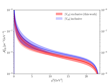
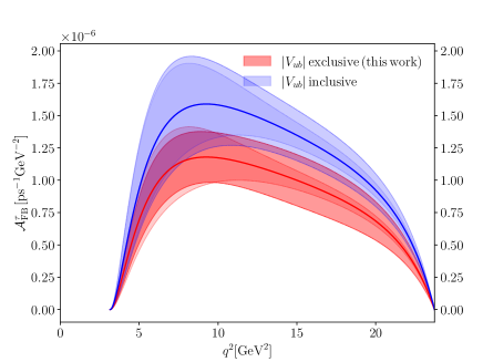
Figure 7: Forward-backward asymmetries $\mathcal{A}_{\rm FB}^{\mu}$ (left) and $\mathcal{A}_{\rm FB}^{\tau}$ (right). For $|V_{ub}|$ exclusive we take our determination (cf. Eq. (38)). The value for $|V_{ub}|$ inclusive is taken from Eq. (41). The inner shading does not include the uncertainty contributions from $|V_{ub}|$.

Furthermore, we define the integrated forward-backward asymmetry $I[\mathcal{A}_{\rm FB}]$ and the average forward-backward asymmetry $\bar{\mathcal{A}}_{\rm FB}$ as

$$I[\mathcal{A}^{\ell}_{\rm FB}]=\int\limits_{m_{\ell}^{2}}^{q^{2}_{\rm max}}dq^{2}\mathcal{A}^{\ell}_{\rm FB}(q^{2})/|V_{ub}|^{2}\,,$$ (96)

and

$$\mathcal{\bar{A}}^{\ell}_{\rm FB}=\frac{\int_{m_{\ell}^{2}}^{q_{\rm max}^{2}}dq^{2}\mathcal{A}^{\ell}_{\rm FB}(q^{2})}{\int_{m_{\ell}^{2}}^{q_{\rm max}^{2}}dq^{2}d\Gamma(B_{s}\to K\ell\nu)/dq^{2}}\,.$$ (97)

Numerical results for these values are provided in Tab. 9.

Another observable which can be computed from the form factor parameterisation is the polarisation asymmetry $\mathcal{A}^{\ell}_{\rm pol}$. This is defined to be the difference between the left-handed and the right-handed contributions to the decay rate Meissner:2013pba ,

$$\mathcal{A}^{\ell}_{\rm pol}(q^{2})=\frac{d\Gamma(\ell,{\rm LH})}{dq^{2}}-\frac{d\Gamma(\ell,{\rm RH})}{dq^{2}}\,,$$ (98)

and can be used to probe for helicity-violating interactions. In the SM this takes the form

$$\frac{d\Gamma(\ell,{\rm LH})}{dq^{2}}= \frac{\eta_{EW}G_{F}^{2}|V_{ub}|^{2}|{\bf p}_{K}|^{3}}{24\pi^{3}}\left(1-\frac{m_{\ell}^{2}}{q^{2}}\right)^{2}f_{+}^{2}(q^{2})\,,$$

$$\frac{d\Gamma(\ell,{\rm RH})}{dq^{2}}= \frac{\eta_{EW}G_{F}^{2}|V_{ub}|^{2}|{\bf p}_{K}|}{24\pi^{3}}\frac{m_{\ell}^{2}}{q^{2}}\left(1-\frac{m_{\ell}^{2}}{q^{2}}\right)^{2}\left(\frac{3}{8}\frac{(M_{B_{s}}^{2}-M_{K}^{2})^{2}}{M_{B_{s}}^{2}}f_{0}^{2}(q^{2})+\frac{|{\bf p}_{K}|^{2}}{2}f_{+}^{2}(q^{2})\right)\,.\quad$$

The polarisation distribution is shown in Fig. 8. Finally, using analogous definitions to Eqs. (96) and (97) we define $I[\mathcal{A}^{\ell}_{\rm pol}]$ and $\mathcal{\bar{A}}^{\ell}_{\rm pol}$ and provide numerical values in Tab. 9.

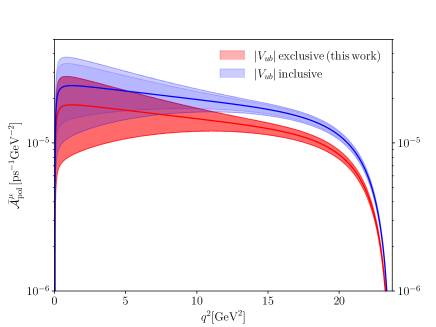
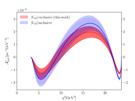
Figure 8: Polarisation asymmetries $\mathcal{A}_{\rm pol}^{\mu}$ (left) and $\mathcal{A}_{\rm pol}^{\tau}$ (right). We again take the value for $|V_{ub}|$ exclusive from Eq. (38) and the value for $|V_{ub}|$ inclusive from Eq. (41). The inner shading does not include the uncertainties of the CKM matrix element.

Appendix F Further numerical results

F.1 Results for observables from Bayesian fits to individual lattice data sets

The results for observables computed from the Bayesian-inference fit to RBC/UKQCD 23 can be found in Tab. 5.4, the ones for FNAL/MILC 19 in Tab. 5.4, and the ones for HPQCD 14 in Tab. 5.4. The corresponding BGL coefficients are listed in Tabs. 5 and 6.

$K_{+}$	$K_{0}$	$I[\mathcal{A}_{\rm FB}^{\tau}]\,[\frac{1}{\rm ps}]$	$I[\mathcal{A}_{\rm FB}^{\mu}]\,[\frac{1}{\rm ps}]$	$\mathcal{\bar{A}}_{\rm FB}^{\tau}$	$\mathcal{\bar{A}}_{\rm FB}^{\mu}$	$I[\mathcal{A}_{\rm pol}^{\tau}]\,[\frac{1}{\rm ps}]$	$I[\mathcal{A}_{\rm pol}^{\mu}]\,[\frac{1}{\rm ps}]$	$\mathcal{\bar{A}}_{\rm pol}^{\tau}$	$\mathcal{\bar{A}}_{\rm pol}^{\mu}$
2	2	1.46(12)	0.0320(46)	0.2720(21)	0.00440(27)	0.794(92)	7.16(68)	0.148(13)	0.98768(73)
2	3	0.99(14)	0.0115(41)	0.2679(27)	0.00284(46)	0.31(13)	3.90(80)	0.082(27)	0.9912(11)
3	2	1.23(13)	0.0315(46)	0.2825(28)	0.00560(44)	0.14(15)	5.53(71)	0.031(34)	0.9838(13)
3	3	1.27(23)	0.038(19)	0.2836(77)	0.0058(15)	0.13(16)	6.0(1.7)	0.030(35)	0.9833(39)
3	4	1.28(27)	0.040(26)	0.2833(91)	0.0057(19)	0.14(17)	6.1(2.2)	0.030(38)	0.9834(49)
4	3	1.29(26)	0.038(19)	0.2820(80)	0.0058(16)	0.18(31)	6.2(2.0)	0.034(65)	0.9832(45)
4	4	1.28(28)	0.039(25)	0.2817(93)	0.0058(20)	0.16(31)	6.2(2.4)	0.031(64)	0.9833(52)
5	5	1.30(28)	0.040(24)	0.2821(89)	0.0057(18)	0.18(29)	6.3(2.3)	0.035(60)	0.9834(49)
6	6	1.31(28)	0.041(24)	0.2826(88)	0.0058(18)	0.19(29)	6.4(2.3)	0.036(58)	0.9832(48)
7	7	1.33(28)	0.043(24)	0.2831(85)	0.0060(18)	0.20(31)	6.6(2.4)	0.037(62)	0.9829(47)
8	8	1.34(29)	0.043(25)	0.2827(86)	0.0059(18)	0.23(32)	6.7(2.5)	0.042(64)	0.9831(47)
9	9	1.35(31)	0.045(27)	0.2830(90)	0.0060(18)	0.23(34)	6.8(2.6)	0.041(67)	0.9827(49)
10	10	1.37(31)	0.047(27)	0.2832(93)	0.0062(18)	0.23(36)	7.0(2.7)	0.040(69)	0.9823(49)

Table 11: Results for observables from Bayesian-inference fit to RBC/UKQCD 23 Flynn:2023nhi .

$K_{+}$	$K_{0}$	$I[\mathcal{A}_{\rm FB}^{\tau}]\,[\frac{1}{\rm ps}]$	$I[\mathcal{A}_{\rm FB}^{\mu}]\,[\frac{1}{\rm ps}]$	$\mathcal{\bar{A}}_{\rm FB}^{\tau}$	$\mathcal{\bar{A}}_{\rm FB}^{\mu}$	$I[\mathcal{A}_{\rm pol}^{\tau}]\,[\frac{1}{\rm ps}]$	$I[\mathcal{A}_{\rm pol}^{\mu}]\,[\frac{1}{\rm ps}]$	$\mathcal{\bar{A}}_{\rm pol}^{\tau}$	$\mathcal{\bar{A}}_{\rm pol}^{\mu}$
2	2	0.884(89)	0.0132(34)	0.2589(36)	0.00305(41)	0.715(83)	4.24(54)	0.210(17)	0.9914(11)
2	3	1.02(10)	0.0217(52)	0.2592(36)	0.00387(44)	0.94(11)	5.48(73)	0.239(17)	0.9895(12)
3	2	0.844(89)	0.0128(34)	0.2619(38)	0.00322(45)	0.578(97)	3.88(54)	0.179(22)	0.9908(12)
3	3	0.98(11)	0.0209(53)	0.2615(40)	0.00396(48)	0.82(13)	5.15(76)	0.218(23)	0.9891(13)
3	4	0.82(13)	0.0122(60)	0.2510(80)	0.00278(82)	0.81(13)	4.13(85)	0.250(31)	0.9923(22)
4	3	0.78(15)	0.0098(64)	0.2476(99)	0.00236(92)	0.80(13)	3.81(93)	0.257(35)	0.9934(25)
4	4	0.79(16)	0.0121(97)	0.248(11)	0.0027(13)	0.80(13)	4.0(1.1)	0.255(34)	0.9924(34)
5	5	0.79(16)	0.0117(90)	0.248(10)	0.0027(12)	0.80(13)	3.9(1.1)	0.255(34)	0.9925(33)
6	6	0.80(16)	0.0121(92)	0.249(10)	0.0027(13)	0.80(14)	4.0(1.1)	0.253(34)	0.9924(33)
7	7	0.80(16)	0.0125(98)	0.249(10)	0.0028(13)	0.80(14)	4.0(1.1)	0.252(35)	0.9923(34)
8	8	0.81(16)	0.013(10)	0.250(10)	0.0029(13)	0.80(13)	4.1(1.2)	0.250(35)	0.9920(35)
9	9	0.83(17)	0.014(11)	0.251(10)	0.0029(13)	0.81(14)	4.2(1.2)	0.250(34)	0.9918(36)
10	10	0.84(17)	0.015(12)	0.252(10)	0.0031(14)	0.81(14)	4.3(1.3)	0.246(34)	0.9914(38)

Table 12: Results for observables from Bayesian-inference fit to FNAL/MILC 19 Bazavov:2019aom .

$K_{+}$	$K_{0}$	$I[\mathcal{A}_{\rm FB}^{\tau}]\,[\frac{1}{\rm ps}]$	$I[\mathcal{A}_{\rm FB}^{\mu}]\,[\frac{1}{\rm ps}]$	$\mathcal{\bar{A}}_{\rm FB}^{\tau}$	$\mathcal{\bar{A}}_{\rm FB}^{\mu}$	$I[\mathcal{A}_{\rm pol}^{\tau}]\,[\frac{1}{\rm ps}]$	$I[\mathcal{A}_{\rm pol}^{\mu}]\,[\frac{1}{\rm ps}]$	$\mathcal{\bar{A}}_{\rm pol}^{\tau}$	$\mathcal{\bar{A}}_{\rm pol}^{\mu}$
2	2	1.22(13)	0.0278(51)	0.2708(37)	0.00443(34)	0.74(15)	6.15(75)	0.164(29)	0.98767(96)
2	3	1.26(14)	0.0314(70)	0.2709(38)	0.00465(44)	0.81(18)	6.59(96)	0.173(31)	0.9872(12)
3	2	1.23(13)	0.0319(59)	0.2780(43)	0.00524(51)	0.46(19)	5.99(76)	0.103(40)	0.9852(15)
3	3	1.36(15)	0.045(10)	0.2814(48)	0.00612(66)	0.53(20)	7.2(1.1)	0.110(40)	0.9830(18)
3	4	1.37(17)	0.046(14)	0.2814(50)	0.00611(83)	0.53(22)	7.3(1.3)	0.109(41)	0.9830(22)
4	3	1.37(15)	0.046(10)	0.2815(50)	0.00616(71)	0.53(22)	7.2(1.1)	0.109(42)	0.9829(20)
4	4	1.36(19)	0.046(21)	0.2810(69)	0.0060(15)	0.53(21)	7.2(1.7)	0.109(42)	0.9834(41)
5	5	1.35(19)	0.044(20)	0.2806(67)	0.0058(15)	0.53(22)	7.1(1.6)	0.109(44)	0.9837(39)
6	6	1.35(20)	0.044(20)	0.2803(69)	0.0058(15)	0.53(22)	7.1(1.7)	0.111(44)	0.9838(39)
7	7	1.35(20)	0.045(20)	0.2806(69)	0.0059(15)	0.53(21)	7.2(1.7)	0.111(43)	0.9835(39)
8	8	1.36(20)	0.045(20)	0.2808(69)	0.0059(15)	0.53(22)	7.2(1.7)	0.109(44)	0.9835(39)
9	9	1.36(20)	0.047(21)	0.2812(71)	0.0060(15)	0.53(22)	7.3(1.7)	0.109(44)	0.9832(40)
10	10	1.37(21)	0.048(23)	0.2815(72)	0.0061(15)	0.53(22)	7.4(1.8)	0.109(43)	0.9831(41)

Table 13: Results for observables from Bayesian-inference fit to HPQCD 14 Bouchard:2014ypa .

F.2 Combined frequentist fit to HPQCD 14, FNAL/MILC 19 and RBC/UKQCD 23

The results for the BGL coefficients from the combined frequentist fit to HPQCD 14, FNAL/MILC 19 and RBC/UKQCD 23 can be found in Tab. 5.4. Judging from the $p$-value no acceptable combined fit over the three data sets is possible.

$K_{+}$	$K_{0}$	$a_{+,0}$	$a_{+,1}$	$a_{+,2}$	$a_{+,3}$	$a_{+,4}$	$a_{+,5}$	$a_{+,6}$	$a_{+,7}$	$p$	$\chi^{2}/N_{\rm dof}$	$N_{\rm dof}$
2	2	0.02641(58)	-0.0824(26)	-	-	-	-	-	-	0.00	5.15	14
2	3	0.02668(68)	-0.0811(31)	-	-	-	-	-	-	0.00	5.50	13
3	2	0.02477(68)	-0.0829(26)	0.054(12)	-	-	-	-	-	0.00	3.95	13
3	3	0.02534(73)	-0.0792(31)	0.062(12)	-	-	-	-	-	0.00	3.89	12
3	4	0.02534(73)	-0.0781(34)	0.067(14)	-	-	-	-	-	0.00	4.19	11
4	3	0.02535(73)	-0.0776(38)	0.074(20)	0.023(30)	-	-	-	-	0.00	4.19	11
4	4	0.02592(97)	-0.033(50)	0.69(69)	2.1(2.3)	-	-	-	-	0.00	4.53	10
5	5	0.0266(10)	0.052(65)	2.21(97)	11.1(5.6)	17.2(15.1)	-	-	-	0.00	5.04	8

$K_{+}$	$K_{0}$	$a_{0,0}$	$a_{0,1}$	$a_{0,2}$	$a_{0,3}$	$a_{0,4}$	$a_{0,5}$	$a_{0,6}$	$a_{0,7}$	$p$	$\chi^{2}/N_{\rm dof}$	$N_{\rm dof}$
2	2	0.0854(17)	-0.2565(75)	-	-	-	-	-	-	0.00	5.15	14
2	3	0.0856(18)	-0.2527(91)	0.021(27)	-	-	-	-	-	0.00	5.50	13
3	2	0.0858(18)	-0.2501(77)	-	-	-	-	-	-	0.00	3.95	13
3	3	0.0864(18)	-0.2379(95)	0.061(28)	-	-	-	-	-	0.00	3.89	12
3	4	0.0869(19)	-0.231(13)	0.067(29)	-0.08(10)	-	-	-	-	0.00	4.19	11
4	3	0.0869(19)	-0.229(15)	0.091(48)	-	-	-	-	-	0.00	4.19	11
4	4	0.0887(27)	-0.08(17)	2.2(2.4)	7.0(7.9)	-	-	-	-	0.00	4.53	10
5	5	0.0887(28)	0.07(20)	6.1(3.3)	41.5(19.0)	93.3(44.0)	-	-	-	0.00	5.04	8

Table 14: Results for the frequentist BGL fit to HPQCD 14 Bouchard:2014ypa , FNAL/MILC 19 Bazavov:2019aom and RBC/UKQCD 23 Flynn:2023nhi . The tables show the results for BGL coefficients for different orders of the fit. Results for higher truncations are possible in principle (i.e. up to ($K_{+},K_{0})=(8,8)$), but higher-order fluctuate wildly – we removed these results from the tables.

F.3 Combined Bayesian fit to RBC/UKQCD 23, HPQCD 14 and Khodjamirian 17

Results for the BGL coefficients of the combined frequentist fit over lattice results by RBC/UKQCD 23, HPQCD 14 and sum-rule results by Khodjamirian 17 can be found in Tab. 5.4, the corresponding results for the Bayesian-inference fit in Tab. 5.4, and results for phenomenology from the Bayesian fit in Tab. 17.

$K_{+}$	$K_{0}$	$a_{0,0}$	$a_{0,1}$	$a_{0,2}$	$a_{0,3}$	$a_{0,4}$	$a_{0,5}$	$p$	$\chi^{2}/N_{\rm dof}$	$N_{\rm dof}$
2	2	0.0985(25)	-0.259(10)	-	-	-	-	0.00	5.60	9
2	3	0.0984(25)	-0.256(11)	0.015(31)	-	-	-	0.00	6.27	8
3	2	0.0982(25)	-0.246(10)	-	-	-	-	0.01	2.47	8
3	3	0.0970(25)	-0.220(12)	0.139(37)	-	-	-	0.63	0.76	7
3	4	0.0966(27)	-0.223(13)	0.159(51)	0.13(23)	-	-	0.55	0.83	6
4	3	0.0970(25)	-0.220(12)	0.140(37)	-	-	-	0.53	0.85	6
4	4	0.0956(28)	-0.226(14)	0.194(61)	0.34(30)	-	-	0.56	0.78	5
5	5	0.0956(33)	-0.22(13)	0.2(1.2)	0.2(3.0)	-1.0(29.7)	-	0.29	1.25	3
6	6	0.0951(35)	-0.12(19)	1.7(2.2)	3.3(4.7)	-36.7(55.0)	-132.6(164.5)	0.31	1.04	1

Table 15: Results for the frequentist BGL fit to HPQCD 14 Bouchard:2014ypa , RBC/UKQCD 23 Flynn:2023nhi and Khodjamirian 17 Khodjamirian:2017fxg . The tables show the results for BGL coefficients for different orders of the fit.

$K_{+}$	$K_{0}$	$a_{0,0}$	$a_{0,1}$	$a_{0,2}$	$a_{0,3}$	$a_{0,4}$	$a_{0,5}$	$a_{0,6}$	$a_{0,7}$	$a_{0,8}$	$a_{0,9}$
2	2	0.0985(25)	-0.258(10)	-	-	-	-	-	-	-	-
2	3	0.0983(25)	-0.256(11)	0.014(31)	-	-	-	-	-	-	-
3	2	0.0982(25)	-0.245(10)	-	-	-	-	-	-	-	-
3	3	0.0970(25)	-0.220(12)	0.140(36)	-	-	-	-	-	-	-
3	4	0.0965(27)	-0.224(13)	0.157(50)	0.13(23)	-	-	-	-	-	-
4	3	0.0970(25)	-0.220(12)	0.140(36)	-	-	-	-	-	-	-
4	4	0.0955(28)	-0.226(14)	0.191(60)	0.33(29)	-	-	-	-	-	-
5	5	0.0958(28)	-0.225(13)	0.193(66)	0.28(28)	-0.15(63)	-	-	-	-	-
6	6	0.0958(28)	-0.225(13)	0.191(68)	0.26(27)	-0.19(61)	0.19(64)	-	-	-	-
7	7	0.0958(28)	-0.225(14)	0.197(70)	0.24(26)	-0.29(65)	0.32(71)	-0.23(66)	-	-	-
8	8	0.0958(28)	-0.224(13)	0.200(72)	0.23(26)	-0.38(68)	0.48(88)	-0.42(90)	0.25(72)	-	-
9	9	0.0959(28)	-0.224(13)	0.205(75)	0.21(25)	-0.46(72)	0.7(1.1)	-0.7(1.2)	0.5(1.1)	-0.24(77)	-
10	10	0.0959(27)	-0.223(14)	0.210(79)	0.19(25)	-0.56(80)	0.9(1.3)	-1.1(1.7)	0.9(1.8)	-0.6(1.4)	0.25(84)

Table 16: Results for the Bayesian-inference BGL fit to HPQCD 14 Bouchard:2014ypa , RBC/UKQCD 23 Flynn:2023nhi and Khodjamirian 17 Khodjamirian:2017fxg . The tables show the results for BGL coefficients for different orders of the fit.

$K_{+}$	$K_{0}$	$f(q^{2}=0)$	$R_{B_{s}\to K}^{\rm impr}$	$R_{B_{s}\to K}$	$\frac{\Gamma^{\tau}}{|V_{ub}|^{2}}\,[\frac{1}{\rm ps}]$	$\frac{\Gamma^{\mu}}{|V_{ub}|^{2}}\,[\frac{1}{\rm ps}]$	$V^{\rm low}_{\rm CKM}$	$V^{\rm high}_{\rm CKM}$	$V^{\rm full}_{\rm CKM}$
2	2	0.255(13)	1.547(15)	0.705(11)	5.58(29)	7.92(48)	0.00321(27)	0.00318(27)	0.00319(26)
2	3	0.261(17)	1.542(19)	0.699(18)	5.64(32)	8.08(59)	0.00315(29)	0.00315(27)	0.00315(27)
3	2	0.268(13)	1.693(37)	0.728(14)	4.88(29)	6.70(49)	0.00328(28)	0.00356(31)	0.00341(28)
3	3	0.322(19)	1.683(35)	0.665(20)	5.12(31)	7.71(59)	0.00287(26)	0.00348(31)	0.00313(27)
3	4	0.326(21)	1.677(39)	0.659(24)	5.09(32)	7.75(62)	0.00285(27)	0.00349(33)	0.00312(28)
4	3	0.323(20)	1.692(41)	0.668(21)	5.08(32)	7.62(62)	0.00289(26)	0.00351(31)	0.00315(27)
4	4	0.335(23)	1.687(40)	0.652(25)	4.98(33)	7.65(61)	0.00284(27)	0.00354(33)	0.00312(27)
5	5	0.335(22)	1.688(44)	0.653(26)	5.01(34)	7.69(67)	0.00284(27)	0.00354(33)	0.00313(28)
6	6	0.333(22)	1.688(42)	0.654(26)	5.01(33)	7.67(64)	0.00284(27)	0.00353(33)	0.00311(28)
7	7	0.333(22)	1.685(43)	0.653(26)	5.02(33)	7.70(65)	0.00284(27)	0.00353(33)	0.00312(28)
8	8	0.333(22)	1.687(43)	0.653(26)	5.02(33)	7.70(65)	0.00283(27)	0.00352(31)	0.00312(27)
9	9	0.334(22)	1.685(43)	0.653(26)	5.04(33)	7.74(66)	0.00283(27)	0.00351(33)	0.00311(28)
10	10	0.334(22)	1.686(43)	0.652(26)	5.05(32)	7.76(64)	0.00282(27)	0.00352(32)	0.00310(27)

$K_{+}$	$K_{0}$	$I[\mathcal{A}_{\rm FB}^{\tau}]\,[\frac{1}{\rm ps}]$	$I[\mathcal{A}_{\rm FB}^{\mu}]\,[\frac{1}{\rm ps}]$	$\mathcal{\bar{A}}_{\rm FB}^{\tau}$	$\mathcal{\bar{A}}_{\rm FB}^{\mu}$	$I[\mathcal{A}_{\rm pol}^{\tau}]\,[\frac{1}{\rm ps}]$	$I[\mathcal{A}_{\rm pol}^{\mu}]\,[\frac{1}{\rm ps}]$	$\mathcal{\bar{A}}_{\rm pol}^{\tau}$	$\mathcal{\bar{A}}_{\rm pol}^{\mu}$
2	2	1.537(82)	0.0390(32)	0.2753(15)	0.00492(16)	0.800(75)	7.81(47)	0.143(11)	0.98633(45)
2	3	1.552(88)	0.0402(41)	0.2752(15)	0.00497(19)	0.83(10)	7.97(58)	0.147(14)	0.98623(49)
3	2	1.388(83)	0.0400(33)	0.2846(19)	0.00597(28)	0.22(12)	6.59(48)	0.044(23)	0.98300(84)
3	3	1.474(87)	0.0528(52)	0.2882(22)	0.00685(35)	0.24(12)	7.56(58)	0.047(22)	0.98077(99)
3	4	1.467(90)	0.0535(56)	0.2880(23)	0.00690(37)	0.26(13)	7.60(61)	0.050(24)	0.9807(10)
4	3	1.465(91)	0.0527(53)	0.2883(22)	0.00691(39)	0.22(13)	7.47(61)	0.042(25)	0.9806(11)
4	4	1.436(92)	0.0550(59)	0.2884(23)	0.00720(49)	0.22(13)	7.49(60)	0.044(25)	0.9798(14)
5	5	1.446(97)	0.0552(59)	0.2885(23)	0.00718(49)	0.22(14)	7.54(66)	0.043(27)	0.9799(14)
6	6	1.444(93)	0.0548(58)	0.2885(23)	0.00715(49)	0.22(14)	7.51(63)	0.043(26)	0.9799(14)
7	7	1.449(93)	0.0549(59)	0.2884(23)	0.00713(48)	0.23(14)	7.55(64)	0.045(26)	0.9800(14)
8	8	1.449(92)	0.0550(58)	0.2885(23)	0.00714(48)	0.23(14)	7.55(63)	0.044(26)	0.9800(14)
9	9	1.455(94)	0.0552(59)	0.2885(23)	0.00713(48)	0.23(14)	7.59(65)	0.045(26)	0.9800(14)
10	10	1.456(90)	0.0553(59)	0.2887(24)	0.00713(48)	0.23(14)	7.60(63)	0.045(27)	0.9800(14)

Table 17: Summary of results based on combined fit to HPQCD 14 Bouchard:2014ypa , RBC/UKQCD 23 Flynn:2023nhi and Khodjamirian 17 Khodjamirian:2017fxg . Definitions for the asymmetries $\mathcal{A}$ can be found in App. E.

References

- (1) N. Gubernari, D. van Dyk, and J. Virto, Non-local matrix elements in , JHEP 02 (2021) 088, [arXiv:2011.09813].
- (2) N. Gubernari, M. Reboud, D. van Dyk, and J. Virto, Improved theory predictions and global analysis of exclusive processes, JHEP 09 (2022) 133, [arXiv:2206.03797].
- (3) T. Blake, S. Meinel, M. Rahimi, and D. van Dyk, Dispersive bounds for local form factors in transitions, Phys. Rev. D 108 (2023), no. 9 094509, [arXiv:2205.06041].
- (4) Particle Data Group Collaboration, R. L. Workman and Others, Review of Particle Physics, PTEP 2022 (2022) 083C01.
- (5) Flavour Lattice Averaging Group (FLAG) Collaboration, Y. Aoki et al., FLAG Review 2021, Eur. Phys. J. C 82 (2022), no. 10 869, [arXiv:2111.09849].
- (6) P. Colangelo and A. Khodjamirian, QCD sum rules, a modern perspective, hep-ph/0010175.
- (7) A. Khodjamirian, Hadron Form Factors: From Basic Phenomenology to QCD Sum Rules. CRC Press, Taylor & Francis Group, Boca Raton, FL, USA, 2020.
- (8) C. G. Boyd, B. Grinstein, and R. F. Lebed, Constraints on form-factors for exclusive semileptonic heavy to light meson decays, Phys. Rev. Lett. 74 (1995) 4603–4606, [hep-ph/9412324].
- (9) I. Caprini, L. Lellouch, and M. Neubert, Dispersive bounds on the shape of form-factors, Nucl. Phys. B530 (1998) 153–181, [hep-ph/9712417].
- (10) C. Bourrely, I. Caprini, and L. Lellouch, Model-independent description of decays and a determination of , Phys. Rev. D79 (2009) 013008, [arXiv:0807.2722]. erratum: Phys. Rev. D82 (2010) 099902.
- (11) W. W. Buck and R. F. Lebed, New constraints on dispersive form-factor parameterizations from the timelike region, Phys. Rev. D 58 (1998) 056001, [hep-ph/9802369].
- (12) T. Becher and R. J. Hill, Comment on form-factor shape and extraction of from , Phys. Lett. B633 (2006) 61–69, [hep-ph/0509090].
- (13) C. Bourrely, B. Machet, and E. de Rafael, Semileptonic decays of pseudoscalar particles () and short distance behaviour of quantum chromodynamics, Nucl. Phys. B189 (1981) 157–181.
- (14) L. Lellouch, Lattice constrained unitarity bounds for decays, Nucl. Phys. B479 (1996) 353–391, [hep-ph/9509358].
- (15) M. Di Carlo, G. Martinelli, M. Naviglio, F. Sanfilippo, S. Simula, and L. Vittorio, Unitarity bounds for semileptonic decays in lattice QCD, Phys. Rev. D 104 (2021), no. 5 054502, [arXiv:2105.02497].
- (16) A. Jüttner, BFF – Bayesian Form factor Fit code https://github.com/andreasjuettner/BFF, https://doi.org/10.5281/zenodo.7799543, .
- (17) L. Del Debbio, T. Giani, and M. Wilson, Bayesian approach to inverse problems: an application to NNPDF closure testing, Eur. Phys. J. C 82 (2022), no. 4 330, [arXiv:2111.05787].
- (18) E. T. Neil and J. W. Sitison, Improved information criteria for Bayesian model averaging in lattice field theory, Phys. Rev. D 109 (2024), no. 1 014510, [arXiv:2208.14983].
- (19) W. I. Jay and E. T. Neil, Bayesian model averaging for analysis of lattice field theory results, Phys. Rev. D 103 (2021) 114502, [arXiv:2008.01069].
- (20) J. Frison, Towards fully bayesian analyses in Lattice QCD, arXiv:2302.06550.
- (21) C. Duhr, A. Huss, A. Mazeliauskas, and R. Szafron, An analysis of Bayesian estimates for missing higher orders in perturbative calculations, JHEP 09 (2021) 122, [arXiv:2106.04585].
- (22) C. Bouchard, G. P. Lepage, C. Monahan, H. Na, and J. Shigemitsu, form factors from lattice QCD, Phys.Rev. D90 (2014), no. 5 054506, [arXiv:1406.2279].
- (23) Fermilab Lattice/MILC Collaboration, A. Bazavov et al., decay from lattice QCD, Phys. Rev. D100 (2019), no. 3 034501, [arXiv:1901.02561].
- (24) RBC/UKQCD Collaboration, J. M. Flynn, R. C. Hill, A. Jüttner, A. Soni, J. T. Tsang, and O. Witzel, Exclusive semileptonic decays on the lattice, Phys. Rev. D 107 (2023), no. 11 114512, [arXiv:2303.11280].
- (25) A. Khodjamirian and A. V. Rusov, and decays at large recoil and CKM matrix elements, JHEP 08 (2017) 112, [arXiv:1703.04765].
- (26) LHCb Collaboration, R. Aaij et al., First observation of the decay and Measurement of , Phys. Rev. Lett. 126 (2021), no. 8 081804, [arXiv:2012.05143].
- (27) LHCb Collaboration, R. Aaij et al., Measurement of with decays, Phys. Rev. D 101 (2020), no. 7 072004, [arXiv:2001.03225].
- (28) HPQCD Collaboration, H. Na, C. M. Bouchard, G. P. Lepage, C. Monahan, and J. Shigemitsu, form factors at nonzero recoil and extraction of , Phys. Rev. D92 (2015), no. 5 054510, [arXiv:1505.03925]. erratum: Phys. Rev. D93 (2016) 119906.
- (29) A. Sirlin, Large , behavior of the corrections to semileptonic processes mediated by , Nucl. Phys. B196 (1982) 83–92.
- (30) J. M. Flynn, T. Izubuchi, T. Kawanai, C. Lehner, A. Soni, R. S. Van de Water, and O. Witzel, and form factors and from -flavor lattice QCD with domain-wall light quarks and relativistic heavy quarks, Phys. Rev. D91 (2015), no. 7 074510, [arXiv:1501.05373].
- (31) C. G. Boyd, B. Grinstein, and R. F. Lebed, Model independent determinations of (lepton), (lepton) anti-neutrino form-factors, Nucl. Phys. B461 (1996) 493–511, [hep-ph/9508211].
- (32) C. G. Boyd and M. J. Savage, Analyticity, shapes of semileptonic form-factors, and , Phys. Rev. D 56 (1997) 303–311, [hep-ph/9702300].
- (33) M. C. Arnesen, B. Grinstein, I. Z. Rothstein, and I. W. Stewart, A precision model independent determination of from , Phys. Rev. Lett. 95 (2005) 071802, [hep-ph/0504209].
- (34) W. A. Bardeen, E. J. Eichten, and C. T. Hill, Chiral multiplets of heavy-light mesons, Phys. Rev. D68 (2003) 054024, [hep-ph/0305049].
- (35) A. Berns and H. Lamm, Model-independent prediction of , JHEP 12 (2018) 114, [arXiv:1808.07360].
- (36) G. Szegö, Orthogonal Polynomials, vol. 23. American Mathematical Society, 1939.
- (37) B. Simon, Orthogonal polynomials on the unit circle: New results, math/0405111.
- (38) G. P. Lepage and S. J. Brodsky, Exclusive processes in perturbative quantum chromodynamics, Phys. Rev. D 22 (1980) 2157.
- (39) R. Akhoury, G. F. Sterman, and Y. P. Yao, Exclusive semileptonic decays of mesons into light mesons, Phys. Rev. D 50 (1994) 358–372.
- (40) H. Jeffreys, The Theory of Probability. Oxford Classic Texts in the Physical Sciences. 1939.
- (41) G. Cossu, L. Del Debbio, A. Jüttner, B. Kitching-Morley, J. K. L. Lee, A. Portelli, H. B. Rocha, and K. Skenderis, Nonperturbative Infrared Finiteness in a Superrenormalizable Scalar Quantum Field Theory, Phys. Rev. Lett. 126 (2021), no. 22 221601, [arXiv:2009.14768].
- (42) G. Duplancic and B. Melic, form factors: An Update of light-cone sum rule results, Phys.Rev. D78 (2008) 054015, [arXiv:0805.4170].
- (43) R. Faustov and V. Galkin, Charmless weak decays in the relativistic quark model, Phys.Rev. D87 (2013), no. 9 094028, [arXiv:1304.3255].
- (44) W.-F. Wang and Z.-J. Xiao, The semileptonic decays in the perturbative QCD approach beyond the leading-order, Phys.Rev. D86 (2012) 114025, [arXiv:1207.0265].
- (45) G. Martinelli, S. Simula, and L. Vittorio, Exclusive semileptonic and decays through unitarity and lattice QCD, JHEP 08 (2022) 022, [arXiv:2202.10285].
- (46) HFLAV Collaboration, Y. S. Amhis et al., Averages of -hadron, -hadron, and -lepton properties as of 2021, arXiv:2206.07501.
- (47) Particle Data Group Collaboration, R. L. Workman et al., Review of Particle Physics, PTEP 2022 (2022) 083C01.
- (48) Fermilab/MILC Collaboration, J. A. Bailey et al., from decays and (2+1)-flavor lattice QCD, Phys. Rev. D92 (2015), no. 1 014024, [arXiv:1503.07839].
- (49) BaBar Collaboration, P. del Amo Sanchez et al., Study of and Decays and Determination of , Phys.Rev. D83 (2011) 032007, [arXiv:1005.3288].
- (50) BaBar Collaboration, J. Lees et al., Branching fraction and form-factor shape measurements of exclusive charmless semileptonic B decays, and determination of , Phys.Rev. D86 (2012) 092004, [arXiv:1208.1253].
- (51) Belle Collaboration, H. Ha et al., Measurement of the decay and determination of , Phys.Rev. D83 (2011) 071101, [arXiv:1012.0090].
- (52) Belle Collaboration, A. Sibidanov et al., Study of Exclusive Decays and Extraction of using Full Reconstruction Tagging at the Belle Experiment, Phys.Rev. D88 (2013), no. 3 032005, [arXiv:1306.2781].
- (53) P. Gambino, P. Giordano, G. Ossola, and N. Uraltsev, Inclusive semileptonic B decays and the determination of , JHEP 10 (2007) 058, [arXiv:0707.2493].
- (54) B. O. Lange, M. Neubert, and G. Paz, Theory of charmless inclusive B decays and the extraction of , Phys. Rev. D 72 (2005) 073006, [hep-ph/0504071].
- (55) J. R. Andersen and E. Gardi, Inclusive spectra in charmless semileptonic B decays by dressed gluon exponentiation, JHEP 01 (2006) 097, [hep-ph/0509360].
- (56) A. X. El-Khadra, Lattice calculation of meson form-factors for semileptonic decays. PhD thesis, UCLA, 1989.
- (57) G. Isidori and O. Sumensari, Optimized lepton universality tests in decays, Eur. Phys. J. C 80 (2020), no. 11 1078, [arXiv:2007.08481].
- (58) M. Freytsis, Z. Ligeti, and J. T. Ruderman, Flavor models for , Phys. Rev. D 92 (2015), no. 5 054018, [arXiv:1506.08896].
- (59) F. U. Bernlochner and Z. Ligeti, Semileptonic decays to excited charmed mesons with and searching for new physics with , Phys. Rev. D 95 (2017), no. 1 014022, [arXiv:1606.09300].
- (60) G. Martinelli, S. Simula, and L. Vittorio, Constraints for the semileptonic form factors from lattice QCD simulations of two-point correlation functions, Phys. Rev. D 104 (2021), no. 9 094512, [arXiv:2105.07851].
- (61) C. G. Boyd, B. Grinstein, and R. F. Lebed, Precision corrections to dispersive bounds on form-factors, Phys. Rev. D56 (1997) 6895–6911, [hep-ph/9705252].
- (62) J. Grigo, J. Hoff, P. Marquard, and M. Steinhauser, Moments of heavy quark correlators with two masses: exact mass dependence to three loops, Nucl. Phys. B864 (2012) 580–596, [arXiv:1206.3418].
- (63) K. G. Chetyrkin, J. H. Kuhn, A. Maier, P. Maierhofer, P. Marquard, M. Steinhauser, and C. Sturm, Charm and bottom quark masses: An update, Phys. Rev. D80 (2009) 074010, [arXiv:0907.2110].
- (64) K. G. Chetyrkin, J. H. Kuhn, and M. Steinhauser, RunDec: A Mathematica package for running and decoupling of the strong coupling and quark masses, Comput. Phys. Commun. 133 (2000) 43–65, [hep-ph/0004189].
- (65) B. Schmidt and M. Steinhauser, CRunDec: a C++ package for running and decoupling of the strong coupling and quark masses, Comput. Phys. Commun. 183 (2012) 1845–1848, [arXiv:1201.6149].
- (66) F. Herren and M. Steinhauser, Version 3 of RunDec and CRunDec, Comput. Phys. Commun. 224 (2018) 333–345, [arXiv:1703.03751].
- (67) A. Bazavov et al., Staggered chiral perturbation theory in the two-flavor case and SU(2) analysis of the MILC data, PoS LATTICE2010 (2010) 083, [arXiv:1011.1792].
- (68) K. Cichy, E. Garcia-Ramos, and K. Jansen, Chiral condensate from the twisted mass Dirac operator spectrum, JHEP 10 (2013) 175, [arXiv:1303.1954].
- (69) C. Alexandrou, A. Athenodorou, K. Cichy, M. Constantinou, D. P. Horkel, K. Jansen, G. Koutsou, and C. Larkin, Topological susceptibility from twisted mass fermions using spectral projectors and the gradient flow, Phys. Rev. D97 (2018), no. 7 074503, [arXiv:1709.06596].
- (70) S. Borsanyi, S. Durr, Z. Fodor, S. Krieg, A. Schafer, E. E. Scholz, and K. K. Szabo, SU(2) chiral perturbation theory low-energy constants from flavor staggered lattice simulations, Phys. Rev. D88 (2013) 014513, [arXiv:1205.0788].
- (71) Budapest-Marseille-Wuppertal Collaboration, S. Dürr et al., Lattice QCD at the physical point meets SU(2) chiral perturbation theory, Phys. Rev. D90 (2014), no. 11 114504, [arXiv:1310.3626].
- (72) P. A. Boyle et al., Low energy constants of SU(2) partially quenched chiral perturbation theory from domain wall QCD, Phys. Rev. D93 (2016), no. 5 054502, [arXiv:1511.01950].
- (73) G. Cossu, H. Fukaya, S. Hashimoto, T. Kaneko, and J.-I. Noaki, Stochastic calculation of the dirac spectrum on the lattice and a determination of chiral condensate in -flavor QCD, PTEP 2016 (2016), no. 9 093B06, [arXiv:1607.01099].
- (74) JLQCD Collaboration, S. Aoki, G. Cossu, H. Fukaya, S. Hashimoto, and T. Kaneko, Topological susceptibility of QCD with dynamical Möbius domain-wall fermions, PTEP 2018 (2018), no. 4 043B07, [arXiv:1705.10906].
- (75) S. Narison, QCD parameter correlations from heavy quarkonia, Int. J. Mod. Phys. A33 (2018), no. 10 1850045, [arXiv:1801.00592]. addendum: Int. J. Mod. Phys.A33,no.10,1850045(2018).
- (76) U.-G. Meißner and W. Wang, , Angular Analysis, S-wave Contributions and , JHEP 01 (2014) 107, [arXiv:1311.5420].