Unsupervised Gait Recognition with
Selective Fusion

Abstract

Previous gait recognition methods primarily trained on labeled datasets, which require painful labeling effort. However, using a pre-trained model on a new dataset without fine-tuning can lead to significant performance degradation. So to make the pre-trained gait recognition model able to be fine-tuned on unlabeled datasets, we propose a new task: Unsupervised Gait Recognition (UGR). We introduce a new cluster-based baseline to solve UGR with cluster-level contrastive learning. But we further find more challenges this task meets. First, sequences of the same person in different clothes tend to cluster separately due to the significant appearance changes. Second, sequences taken from $0^{\circ}$ and $180^{\circ}$ views lack walking postures and do not cluster with sequences taken from other views. To address these challenges, we propose a Selective Fusion method, which includes Selective Cluster Fusion (SCF) and Selective Sample Fusion (SSF). With SCF, we merge matched clusters of the same person wearing different clothes by updating the cluster-level memory bank with a multi-cluster update strategy. And in SSF, we merge sequences taken from front/back views gradually with curriculum learning. Extensive experiments show the effectiveness of our method in improving the rank-1 accuracy in walking with different coats condition and front/back views conditions.

1 Introduction

With the growing intelligent security and safety camera systems, gait recognition has gradually gained more attention and exploration due to its non-contact, long-term, and long-distance recognition properties. Several works [1, 2, 3] attempt to solve gait recognition tasks and have reached significant progress in a laboratory environment. However, gait recognition in a realistic situation will be affected by many factors such as occlusion, dirty label, or labeling, and more. Among them, the problem of labeling is one of the biggest challenge because it demands intensive manual effort to label pairwise data. Moreover, deploying pre-trained models in new test environments without any adaptation often suffers from severe performance deterioration due to the domain gap across different datasets. So it is necessary to train gait recognition models on unlabeled datasets, which saves a lot of human and financial resources.

To realize gait recognition trained with an unlabeled dataset, we introduce a new task called Unsupervised Gait Recognition (abbreviated as UGR) to facilitate the research on training gait recognition models with new unlabeled datasets. And here we focus on using silhouettes as input to conduct gait recognition. When only using silhouettes of human walking sequences as input, due to lacking enough information, we observe two main challenges in UGR, as shown in Figure 1. First, due to the large change in appearance, sequences in different clothes of a subject are hard to gather into one cluster without any label supervision. Second, sequences captured from front/back views, such as views in $0^{\circ}/018^{\circ}/162^{\circ}/180^{\circ}$ in CASIA-B [4], are challenging to gather with sequences taken from other views of the same person because they lack vital information, such as walking postures. Furthermore, these sequences tend to cluster into small groups based on their views or get mixed with sequences of the same perspective from other subjects. So in this paper, we provide methods to overcome them accordingly.

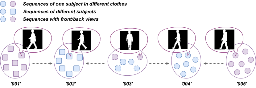
Figure 1: Two main challenges in UGR. A kind of style in different color denotes a subject in different clothes, which are usually erroneously assigned with different pseudo labels (e.g., ‘001’, ‘002’). Also, sequences taken from front/back views of different subjects tend to mix together (e.g., ‘003’).

Currently, some Person Re-identification (Re-ID) works [5, 6, 7, 8, 9, 10] have already touched the field of identifying person in an unsupervised manner. We follow the state-of-the-art pattern in [9], a cluster-based framework with contrastive learning, as a baseline to realize UGR. However, when directly adopting this framework, we find the performance still needs to be improved, especially in the walking with different clothes (CL) condition. To address the two challenges, we propose a new method called Selective Fusion, which comprises two techniques: Selective Cluster Fusion (SCF), which selects candidate clusters of the same subject wearing different clothes and pulls them closer; and Selective Sample Fusion (SSF), which handles front/back view samples of each subject.

To be specific, first, in SCF, we use a support set selection module to generate a support set for each cluster and design a multi-cluster update strategy to help update the cluster centroid of each pseudo cluster in the memory bank. By utilizing this approach, we not only improve the tightness of the clusters themselves but also encourage clusters of the same individual in different clothing to be influenced by the current clustered groups and pulled closer towards them. Second, we design the SSF to deal with samples taken from front/back views. In SSF, we utilize a view classifier to identify sequences captured from front/back views. We then employ curriculum learning to gradually incorporate these sequences with those captured from other views. Namely, the sequences are absorbed at a dynamic rate, relaxing the aggregate requirement for each cluster. This approach enables us to re-assign pseudo labels for sequences captured from front/back views, thereby encouraging them to cluster with sequences captured from other views. With our method, we gain a large recognition accuracy improvement comparing to the baseline (with GaitSet [1] backbone: NM + 3.1%, BG + 8.6%, CL + 9.7%; with GaitGL [3] backbone: BG + 1.1%, GL + 17.2% on CASIA-BN dataset [4]) To sum up, our contributions mainly lie in three folds:

• We introduce a new task Unsupervised Gait Recognition (UGR) for performing gait recognition using unsupervised learning, which is a practical approach but requires careful consideration. To address this task, we establish a baseline that employs cluster-level contrastive learning.

• We deeply explore the characteristic of UGR, finding the two most critical challenges we need to overcome: gathering sequences with different clothes and with front/back views. We propose a Selective Fusion method to tackle the two main problems by select potential matched cluster/sample pairs to help them fuse gradually.

• Extensive experiments on two popular gait recognition benchmarks have shown that our method can bring consistent improvement over baseline, especially in the walking in different coats condition.

2 Related Work

Most existing gait recognition works are trained in a supervised manner, in which cross-cloth and cross-view labeled sequence pairs have been provided. They mainly focus on learning more discriminative features [11, 12, 1, 2, 3, 13, 14, 15, 16] or developing gait recognition applications in natural scenes [17, 18, 19, 20]. Despite the abundance of research in gait recognition, there is still a need for further exploration of its practical applications. Here we consider one practical setting and work as one of the first attempts to realize gait recognition without labeling training datasets.

2.1 Supervised Gait Recognition

Model-based method: This kind of method encodes poses or skeletons into discriminative features to classify identities. For example, PoseGait [11] extracts handcrafted features from 3D poses based on human prior knowledge. JointsGait [12] extracts spatio-temporal features from 2D joints by GCN [21], then map them into discriminative space according to the human body structure and walking pattern. GaitGraph [22] use human pose estimation to extract robust pose from RGB images, and encode the keypoint as node and joints as skeleons in the Graph Convolutional Network to extract gait information.

Appearance-based method: This series of methods mostly input silhouettes, extracting identity information from the shape and walking postures. GaitSet [1] first extracts frame-level and set-level features from an unordered silhouette set, promoting the set-based method’s development. GaitPart [2] further includes part-level pieces of information, mining details from silhouettes. In contrast, the video-based method GaitGL [3] employs 3D CNN for feature extraction based on temporal knowledge. Our method can be used in appearance-based unsupervised gait recognition. Since our method mainly focuses on realistic gait recognition with a large amount of data, we choose silhouettes as input for its computation saving and robustness. In our framework, we adopt both the set-based method and the video-based method as the backbones to illustrate the generalization of our framework.

2.2 Unsupervised Person Re-identification

Short-term Unsupervised Re-ID: Most fully-unsupervised Re-ID methods estimate pseudo labels for sequences, which can be roughly categorized into the clustering-based and non-clustering-based methods. Clustering-based methods [23, 24, 25, 26] first estimate a pseudo label for each sequence and train the network with sequence similarity. In contrast, non-clustering-based methods [7, 8] regard each image as a a class and use a non-parametric classifier to push each similar image closer and pull all other images further. In total, the accuracy of most non-cluster-based methods do not exceed the latest cluster-based methods, so we use the latter to solve UGR.

At present, there are some typical algorithms in clustering-based methods. BUC [5] utilizes a bottom-up clustering method, gradually clustering samples into a fixed number of clusters. Though there is a need for more flexibility, it is a good starting point. HCT [23] adopts triplet loss to BUC to help learn hard samples. SpCL [6] introduces a self-paced learning strategy and memory bank, gradually making generated sample features closer to reliable cluster centroids. To alleviate the high intra-class variance inside a cluster caused by camera styles, CAP [24] proposes cross-camera proxy contrastive loss to pull instances near their own camera centroids in a cluster. ICE [25] further explores inter-instance relationships instead of using camera labels to compact the clusters with hard contrastive loss and soft instance consistency loss. IICS [26] also considers the difference caused by cameras, decomposing the training pipeline into two phases. First, considering each camera as a domain, IICS categorizes features within every single camera and generates intra-camera labels. Second, according to sample similarity across cameras, inter-camera pseudo labels will be generated based on all instances. These two stages train CNN alternately to optimize features. Cluster-contrast [9] improves SpCL by establishing cluster-level memory dictionary, optimizing and updating both CNN and memory bank at the cluster level.

Inspired by the simple but elegant structure, we start from the Cluster-contrast framework to solve UGR. However, owing to the cloth-changing complexity and lack of posture in the front/back view, directly applying Cluster-contrast will lead to sequences in different clothes or with front/back views separate into different clusters. As a solution, we design specific modules to gradually merge samples from different clothes and views.

On the contrary, the non-clustering-based methods mainly realize fully-unsupervised Re-ID with similarity-based methods. SSL [7] predicts a soft label for each sample and trains the classification model with softened label distribution. MMCL [8] formulates FUL Re-ID as a multi-label classification task and classifies each sample into multiple classes by considering their self-similarity and neighbor similarity.

Long-term Unsupervised Re-ID: Most FUL Re-ID methods are based on short-term Re-ID datasets, however, gait recognition is a long-term task with cloth-changing, so long-term FUL Re-ID is more similar to UGR. CPC [27] use curriculum learning [28] strategy to incorporate easy and hard samples and gradually relax the clustering criterion. We do not use the same method in SCF, since each cluster mainly contains sequences with one cloth type, and it is better to pull clusters as a whole. In contrast, we use curriculum learning in SSF to distinguishingly deal with sequences in front/back views and re-assign pseudo labels for sequences in these views progressively.

3 Our Method

In this work, we propose a new task called Unsupervised Gait Recognition (UGR), which is practical when dealing with realistic unlabeled gait datasets. In this section, we first formally define our technique. Next, we will show our baseline based on Cluster-contrast [9], trying to solve UGR with an unlabeled trainset. Then, we deeply research the problems faced by UGR and find two challenges to improve the accuracy: sequences in different clothes of the same person tend to form different clusters, and the sequences captured from front/back views are difficult to gather with other views. Based on the two problems, we propose Selective Fusion to gradually merge cross-cloth clusters and sequences taken from front/back views to make samples of each subject gathered tighter. To clarify the narrate, we summarize the symbols we use in Table I.

TABLE I: The definition of important symbols

Symbol	Definition
$\mathcal{X}_{u}/\mathcal{X}_{t}$	Unlabeled training dataset/ Labeled testing dataset
$\mathcal{Y}_{u}/\mathcal{Y}^{\prime}_{u}$	The true/ pseudo label for training dataset
$\mathcal{Y}_{t}$	The true label for testing dataset
$f_{\theta}$	Gait Recognition backbone
$f_{n}/f_{CA}$	Feature of original/cloth augmented sequence
$\mathcal{C}_{k}$	$k$-th cluster center
$M$	neighbors of each sequence search
$s_{up}$	clustering threshold
$\tau$	The temperature hyper-parameter
$m$	The momentum hyper-parameter
$\mathcal{L}_{CNCE}$	ClusterNCE Loss
$\mathcal{C}_{+}/\mathcal{C}_{q}$	The positive/ $q$-th cluster
$\mathcal{C}_{low}$	The lower bound to judge FVC
$\mathcal{S}_{c}/\mathcal{S}_{i}$	The current/initial similarity bound when re-assign pseudo labels for sequences in FVC
$\lambda/\lambda_{base}$	The ratio/base ratio to merge extreme view sequences in each epoch
$\mathcal{C}_{n}/\mathcal{C}_{o}$	The number of new or old clusters in each epoch
$q[:]$	The support set for $q$-th cluster
$k$	The number of candidate clusters

3.1 Problem Formulation

We first define an unlabeled training dataset with cloth-changing as $\mathcal{X}_{u}=\{x_{1},x_{2},...,x_{N}\}$, where $N$ is the total sequence number. Then, we assume its ground truth label is set as $\mathcal{Y}_{u}$, but we cannot obtain it during training. We want to train a gait recognition backbone $f_{\theta}$ to classify these sequences according to their similarity. During evaluation, $f_{\theta}$ will extract features from a labeled test dataset $\{\mathcal{X}_{t},\mathcal{Y}_{t}\}$ and the gallery will rank according to their similarity with the probe, then we gain the rank-1 accuracy for each condition and each view. We aim to train $f_{\theta}$ and gain the best performance on $\mathcal{X}_{t}$.

3.2 Proposed Baseline

Without any supervision, it is not easy to train $f_{\theta}$. Since there is no pre-trained model in the Gait Recognition field like in Re-ID, we choose OUMVLP [29] to train a pre-trained model and gain cross-view prior knowledge, Since OUMVLP has a large number of subjects and various views, which is an ideal dataset to obtain identity classification ability. Then we modify Cluster-contrast [9] to build our baseline framework to transfer the knowledge learned from OUMVLP to other datasets. The training pipeline can be summarized as followings:

1) At the beginning of each epoch, we first use $f_{\theta}$ to extract features from each sequence in parts, which has been sliced by Horizontal Pyramid Matching (HPM) [1] horizontally and equally. Then we concatenate all the parts to an embedding and regard it as a sequence feature to participate in the following process, denoted as $f_{n},\ n\in\{1,2,...,N\}$. In this way, we can consider features in parts and details.

2) We adopt KNN [30] to search $M$ neighbors for each sequence in feature space and calculate the similarity distances between each other. Then InfoMap [31] is used to cluster $f_{n}$ with a similarity threshold $s_{up}$, and predict a pseudo label $\mathcal{Y}^{\prime}_{u}=\{y^{\prime}_{1},y^{\prime}_{2},...,y^{\prime}_{N}\}$ for each sequence. When mapping features with a pre-trained model, each sequence tends to be mapped closer and not well separated. So we tighten $s_{up}$, aiming to separate each subject into single cluster.

3) With the pseudo labels, we compute the centroids of each cluster and then initialize a memory bank at the cluster-level to store these centers.

4) During each iteration, a mini-batch will be randomly selected from pseudo clusters, and during gradient propagation, we update the backbone with a ClusterNCE loss [9].

$$\mathcal{L}_{CNCE}=-\log\frac{\exp\left(f_{n}\cdot\mathcal{C}_{+}/\tau\right)}{\sum_{q=0}^{Q}{\exp}\left(f_{n}\cdot\mathcal{C}_{q}/\tau\right)}$$ (1)

where $Q$ is the cluster number gained in the current epoch, $\mathcal{C}_{+}$ is the positive cluster the feature belonging to, $\mathcal{C}_{q}$ is the $q$-th clusters, $\tau$ is the temperature hyper-parameter. Here we use all the positive features in the mini-batch to calculate $\mathcal{L}_{CNCE}$.

5) Also, we update the memory bank at the cluster-level.

$$\mathcal{C}_{q}\leftarrow m\mathcal{C}_{q}+(1-m)f_{n}$$ (2)

$m$ is the momentum hyper-parameter used to update the centroids impacted by the batch.

With this pipeline, we can initially realize UGR. However, some defects still prevent further improvement in both cross-cloth and cross-view situations. First, each cloth condition of a subject has been separated away from each other, making it hard to group them together into a single class. This is because of the large intra-class diversity within each subject when the identity changes cloth and subtle inter-class variance between different persons when cloth types of different subjects are similar. For example, NM and CL of one person are less similar in appearance to NM of other persons, leading to the intra-similarity being smaller than the inter-similarity. Second, some sequences in front/back views (such as $0^{\circ}/018^{\circ}/162^{\circ}/180^{\circ}$) cannot correctly gather with sequences in other views, but tend to be confused with front/back views sequences of other subjects. This is because sequences in these views lack enough walking patterns, so the model can only use the shape information to classify these sequences. With more similarity in appearance, sequences of different subjects in these views tend to be classified together. Necessary solutions need to be considered to help the framework solve the two problems.

3.3 Proposed Method

To tackle the problems we pointed out for UGR, we develop Selective Fusion, containing Selective Cluster Fusion (SCF) and Selective Sample Fusion (SSF) to solve the two drawbacks separately. The framework of our method is in Figure 2, and the pseudo-code is shown in Algorithm 1.

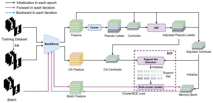
Figure 2: Overview of the framework with Selective Fusion. The upper two branches generate pseudo labels and initialize a memory bank at the start of each epoch. The lower branch accepts mini-batch extracted from pseudo clusters and calculates ClusterNCE Loss with Memory Bank to update it and the backbone in each iteration. CA is the Cloth Augmentation method. InfoMap is employed in the Cluster module. SCF means Selective Cluster Fusion. SSF represents Selective Sample Fusion. In the Support set, the darker the color, the higher the similarity with the target cluster (Best viewed in color).

Algorithm 1 The training procedure of Selective Fusion

Input: $\mathcal{X}_{u}$; $f_{\theta}$

0:  Epoch number; iteration number; batch size; hyper-parameters: $M/s_{up}/\tau/m/\mathcal{C}_{low}/\lambda_{base}/k/\mathcal{S}_{i}$

1:  for epoch in range(0, epoch number+1)  do

2:     Apply CA to $\mathcal{X}_{u}$, get the augmented $\mathcal{X}_{u}$;

3:     Extract $f_{n}$ from $\mathcal{X}_{u}$ by $f_{\theta}$;

4:     Extract $f_{CA}$ from augmented $\mathcal{X}_{u}$ by $f_{\theta}$;

5:     Generate $\mathcal{Y}^{\prime}_{u}$ for $f_{n}$

6:     Calculate the pseudo centroids with $\mathcal{Y}^{\prime}_{u}$ and $f_{n}$;

7:     Generate adjusted $\mathcal{Y}^{\prime}_{u}$ in SSF;

8:     Generate adjusted centroids with adjusted $\mathcal{Y}^{\prime}_{u}$ and $f_{n}$;

9:     Initialize Memory Bank with adjusted centroids;

10:     Generate support set in Support Set Selection Module with the centroids of $f_{CA}$ and $f_{n}$;

11:     for iter in range(0, iteration number+1)  do

12:        Extract mini-batch from pseudo clusters;

13:        Extract sequences feature from batch;

14:        Calculate ClusterNCE loss with Memory Bank according to Eq. 1;

15:        Update the backbone;

16:        Update the Memory Bank according to Eq. 3;

17:     end for

18:  end forOutput: $f_{\theta}$

In our method, at the beginning of each epoch, we use a Cloth Augmentation (CA) method to randomly generate an augmented variant for each sequence in the training dataset, then put them into the same backbone to extract features, named $f_{n}$ and $f_{CA}$. Second, after getting the original pseudo labels generated by InfoMap, we use SSF to adjust the pseudo labels and then apply them to $f_{n}$ and $f_{CA}$ to get their adjusted centroids. The centroids of $f_{n}$ are used to initialize the memory bank. Third, we use a support set selection module to generate a support set for each cluster, which will be used in the multi-cluster update strategy during backpropagation to help update the memory bank. The support set selection module and multi-cluster update strategy are the two components of our SCF.

Next, we will introduce how we implement our Cloth Augmentation, SCF, and SSF method.

3.3.1 Cloth Augmentation

The cloth augmentation is conducted for each sequence in training set to explicitly get a fuse direction for each cluster, which simulates the potential clusters in other conditions belonging to the same person. Currently the cloth augmentation methods we use are target for silhouettes datasets, which are the majority algorithms work on. We randomly dilate or erode the upper/bottom/whole body in the whole sequence with a probability of 0.5, forming six cloth augmentation types. Also, the upper/middle/bottom has a dynamic edited boundary, adding more variance to the augmentation results. Here we visualize some cloth augmented results in Figure 3. When dilating NM, the sequence can simulate its corresponding CL condition, and when eroding CL, the appearance of subjects can be regarded as in NM condition.

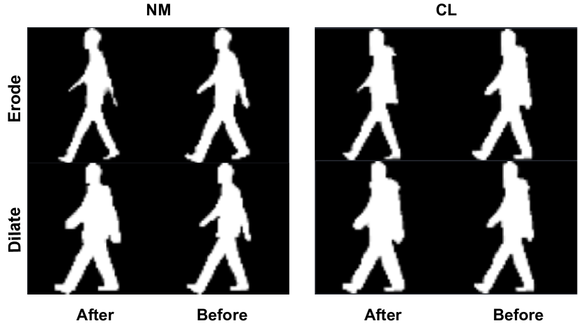
Figure 3: The visualization of data augmentation on NM and CL conditions. Cloth Augmentation can simulate the potential appearance in different conditions of the same person.

It is indeed that in the real-world cloth-changing situations, the clothes have more diversity, only dilating or erode cannot fully simulate all the situations. Currently we first consider the simple cloth-changing situation that walking with or without coats, which is also the cloth-changine method in CASIA-B [4] and Outdoor-Gait [32] dataset, to prove our method is valid. When the situations become complex, other cloth augmentation method can be employed, such as sheer the bottom part of the silhouettes to simulate wearing a dress, adding oval above the head to simulate wearing a hat. But since such real conditions don’t appear in these common datasets, adding more cloth augmentation method will hinder we verify the effectiveness of our method.

3.3.2 Selective Cluster Fusion

SCF aims to pull clusters in different clothes belonging to the same subject closer. It comprises two parts, a support set selection, which is used to generate a support set for each cluster, aiming to find potential candidate clusters in different clothes, and a multi-cluster update strategy, aiming to decrease the distance between candidate clusters in the support set.

Support Set: The input of the support set selection module is the adjusted centroids of $f_{n}$ and $f_{CA}$. By calculating the similarity between the CA centroids of each cluster with the original centroids of $f_{n}$, we can get a rank list with these pseudo labels, ranging from highest to lowest according to their similarity distances. We select the top $k$ ids in each rank list, and the first id we set is the cluster itself, formulating the support set. With the support set, we can concretize the optimization direction when pulling NM and CL together because $f_{CA}$ can be seen as the cross-cloth sequences in reality to some extent. With the explicit regulation, we will not blindly pull a cluster close to any near neighbor.

Multi-cluster update strategy: When updating the memory bank during backpropagating, we use the support set in the multi-cluster update strategy. Knowing which clusters are the potential conditions of one person, the new strategy can be formulated as follows:

$$\mathcal{C}_{q[:k]}\leftarrow m\mathcal{C}_{q[:k]}+(1-m)f_{n}$$ (3)

All the candidate clusters in $q[:k]$ need to participate in updating the memory bank. By forcing the potential conditions to fuse, we can make the mini-batch influence clusters and clusters in the support set, compressing the distance between cross-cloth pairs.

3.3.3 Selective Sample Fusion

Seeing that walking postures are absent in front/back views, sequences taken from these views have less feature similarity with features extracted from other views. So they cannot be appropriately gathered into their clusters like other views, and tend to mix up with sequences of other identities captured from front/back views. If we pull all the clusters towards their candidate clusters in the support set, those clusters mainly composed of sequences taken from front/back views will further gather with clusters with the same view condition, making the situation worse. To deal with clusters in this condition, we design SSF, in which we use curriculum learning to gradually re-assign pseudo labels to sequences in front/back views, forcing them to fuse with samples taken from other views progressively before conducting the SCF method.

View classifer: Specifically, we first train a view classifier on OUMVLP, classifying whether the sequence is in the front/back view. The view classifier structure we set is as same as the GaitSet structure we used, and we add the BNNeck behind. We assign the label 1 for sequences in $0^{\circ}/180^{\circ}$ and assign the label 0 for sequences in other views to train the view classifier. We train the view classifer on OUMVLP to gain view knowledge, and when we have prior knowledge on sequences’ view, we can quickly identify which clusters generated by our framework are composed of sequences taken from front/back views.

Indeed, it is true that when adapting the view classifier to other datasets, there may be appearance domain gaps and view classification gaps between different datasets, as other datasets may not label views in the same way as OUVMLP, and some datasets may not provide view labels at all. But from our observations, we found the view classification task is not a hard task, the view classifier can already identify most sequences with less walking postures. And to further solve the problem that some sequences haven’t appropriately assigned the right view label, we set a threshold to relax the requirement when clustering. The criterion is that only when the number of sequences in front/back view in one cluster is larger than the threshold $\mathcal{C}_{low}$, we consider the cluster as Front/Back View Clusters (FVC). By dissolving FVC, we calculate the similarity between each sequence in it with other centroids of non-FVC, and if the similarity is larger than $\mathcal{S}_{c}$, we re-assign the nearest non-FVC pseudo label for the sequence. So it does not matter whether we identify all the sequences with front/back views. We only need to push most of these sequences closer to other views. And with the training process of curriculum learning, the clusters are tighter. The sequences identified with front/back views will also push the sequences that were misidentified closer to their cluster center automatically since they have appearance similarity. We will further propose more intelligent methods to reduce the dependence of the model on the prior information.

Curriculum Learning: However, we do not incorporate all the sequences in FVC at the same time, instead, we utilize Curriculum Learning [28] to fuse them progressively by enlarging the $\mathcal{S}_{c}$ during each epoch:

$$\mathcal{S}_{c}=\mathcal{S}_{i}-\lambda\times epoch\_number$$ (4)

In the first epoch, $\mathcal{S}_{i}$ is higher, and only the similarity between sequences in FVC and centroids of other non-FVC higher than $\mathcal{S}_{i}$, can these sequences be assigned new pseudo labels. Otherwise, they will be seen as outliers and cannot participate in training. During training, the criterion gradually increases with a speed of $\lambda$, which allows for the gradual incorporation of new knowledge. In response to this, we propose to set $\lambda$ adaptively [33]:

$$\lambda=\lambda_{base}\left|\frac{\mathcal{C}_{n}}{\mathcal{C}_{o}}\right|$$ (5)

where $\mathcal{C}_{n}$ and $\mathcal{C}_{o}$ is the number of new and old clusters in each epoch, $\lambda_{base}$ is a fixed constant for each dataset. Since more clusters fused in each phase, $\lambda$ increases as the ratio of the number of new clusters to that of old clusters increases.

3.4 Training Strategy

Overall, Selective Fusion can make separated conditions and scattered sequences taken from front/back views fuse tighter. Here we show our training strategy and represent the feature distribution of each training phase in Figure 4. Our training strategy encompasses three stages. At first, the features extracted by the pre-trained model have a tendency to cluster together, making it hard to distinguish between them. We adopt our baseline to separate these sequences with a strict criterion, making each cluster gathered according to their similarity. Second, we apply Selective Fusion to fuse different conditions of the same person and gradually merge sequences in front/back views with sequences in other views. Finally, we get the clusters with all the cloth conditions and views.

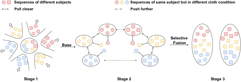
Figure 4: The three stages in our training strategy. First, with narrowed features extracted by pre-trained model, we first adopt our baseline to separate them further. Then Selective Fusion is used to fuse matched clusters and samples together. Finally, we gain clusters with different clothes and views. Base is the Baseline. Each type in different color indicates each subject in different cloth condition.

4 Experiments

Our methods can be employed in appearance-based methods. For simplicity, we take silhouettes sequences as input since they are more robust when datasets are collected in the wild. To demonstrate the effectiveness of our framework, we apply our methods to two existed backbones: GaitSet [1] and GaitGL [3] to help them train with unlabeled datasets. We also compare our method with upper bound which is trained with ground truth label, and with the baseline, which is also trained without supervision. All methods are implemented with PyTorch [34] and trained on TITAN-XP GPUs.

4.1 Datasets

Here we first pre-train backbones on a large gait recognition dataset OUMVLP [29]. Most of the previous unsupervised ReID methods use ResNet-50 [35] pre-trained on ImageNet [36] as the pre-train model, while in gait recognition, there does not exist any pre-train model with strong generalization. Fortunately, OUMVLP contains a large number of subjects with 14 views, which is an ideal dataset to pre-train models. We can train backbones on it to gain preliminary information to classify subjects, and with the large dataset volume, the model can be more generalized when adapted to other datasets. However, without cross-cloth pairs in OUMVLP, the model could only gain cross-view ability. So, we need to develop methods to help the model recognize cross-cloth pairs. We load the pre-trained model and evaluate the performance of our method on two popular datasets, CASIA-BN [4] and Outdoor-Gait [32].

4.1.1 OUMVLP

OUMVLP [29] contains 10,307 subjects. The sequences of each subject distributed in 14 views between $[0^{\circ},90^{\circ}]$ and $[180^{\circ},270^{\circ}]$ but only have normal walking conditions (00, 01). We used 5153 subjects to pre-train backbones. Especially, 00 is used as the gallery, and 01 is taken as the probe. Without walking with different clothes sequences, the model trained on OUMVLP does not have much cross-cloth ability, so we need to develop specific methods to fuse cloth-changing pairs.

4.1.2 CASIA-BN

The original CASIA-B is a useful dataset with both cross-view and cross-cloth sequence pairs. It consists of 124 subjects, having three walking conditions: normal walking (NM#01-NM#06), carrying bags (BG#01-BG#02), and walking with different coats (CL#01-CL#02). Each walking condition contains 11 views distributed in $[0^{\circ},180^{\circ}]$. We employ the protocol in the previous research [1, 2], taking 74 subjects as the training dataset and 50 subjects as the testing dataset. During the evaluation, NM#01-NM#04 are taken as the gallery set, NM#05-NM#06, BG#01-BG#02, CL#01-CL#02 used as the probe. However, since the segmentation of CASIA-B is relatively rough, we collect some pedestrian images and trained a new segmentation model to re-segment CASIA-B, and gain CASIA-BN.

4.1.3 Outdoor-Gait

This dataset only has cross-cloth sequence pairs. With 138 subjects, Outdoor-Gait contains three walking conditions: normal walking (NM#01-NM#04), carrying bags (BG#01-BG#04), and walking with different coats (CL#01-CL#04). There are three capture scenes (Scene#01-Scene#03), however, each person only has one view ($90^{\circ}$). 69 subjects are used for training and the last 69 subjects for tests. During the test, we use NM#01-NM#04 in Scene#03 as gallery and all the sequences in Scene#01-Scene#02 as probe in different conditions.

Noted that during training, we do not use the true label in the training set of both CASIA-BN and Outdoor-Gait.

4.2 Implementation Details

4.2.1 Structure and Optimization Details

Here we show the structure and optimization setting we used in pre-training in Table II and used in unsupervised learning in Table III.

TABLE II: The Parameters used to train a pre-train model on OUMVLP dataset.

Param	Backbone	OUMVLP
Batch Size	GaitSet	(32, 16)
	GaitGL	(32, 8)
Start LR	Both	1e-1
MileStones	GaitSet	[50k, 100k, 125k]
	GaitGL	[150k, 200k, 210k]

TABLE III: The parameters used in unsupervised learning on CASIA-BN and Outdoor-Gait dataset.

Param	Backbone	CASIA-BN	Outdoor-Gait
Model Channel	GaitSet	(32, 64, 128)(128, 256)	(32, 64, 256)(128, 256)
	GaitGL	(32, 64, 128)(128, 128)	-
Batch Size	Both	(8, 16)	(8, 8)
Weight Decay	Both	5e-4	5e-4
Start LR	Both	1e-4	1e-4
MileStones	Both	[3.5k, 8.5k]	[3.5k, 8.5k]
Epoch	Both	Baseline: 50, SF: 50	Baseline: 50, SF: 50
Iteration	Both	Baseline: 50, SF: 100	Baseline: 50, SF: 100
Upper bound Milestones	GaitSet	[20k, 40k, 60k, 80k]	[10k, 20k, 30k, 35k]
	GaitGL	[70k, 80k]	-

The pretrained backbone we use is same for both CASIA-BN and Outdoor-Gait. For the GaitSet backbone, we adopt the GaitSet baseline in OpenGait [37], and for the GaitGL backbone, we also use the GaitGL implementation in OpenGait. When training the view classifier, we adopt the same GaitSet baseline in OpenGait. The input and output channel dimension of each module in GaitSet and GaitGL backbone can be in the first row of Table III.

4.2.2 Hyper-Parameters Setting

During training, we select 30 frames, and use all the frames for evaluation. For the hyper-parameters, we set $s_{up}=0.7$ for baseline, and $s_{up}=0.3$ for Selective Fusion to enlarge the boundary, others are set as $M=40$, $\tau=0.05$, $m=0.2$, $k=2$, $\lambda_{base}=0.005$, $\mathcal{C}_{low}=0.8$, $\mathcal{S}_{i}=0.7$. The experiments conducted for choosing these hyper-parameters can be seen in Section  4.4.1. Since the sequences in Outdoor-Gait is fewer, we change $M$ to 20 to avoid overfitting. Each frame has been normalized to $64\times 44$.

4.2.3 Benchmark settings

To show the effectiveness, we define several benchmarks:

(1) Upper. Upper bound reports the performance of each backbone trained with ground-truth labels.

(2) Pre-train. The effect when directly applying the pre-trained model to the target dataset without fine-tuning.

(3) Base (CC). Fine-tuning the pre-trained model with our baseline framework implemented by Cluster-contrast.

(4) Ours (SF). The results with our proposed method.

4.3 Performance Comparison

Before training and testing on CASIA-BN or Outdoor-Gait, we first pre-train backbones on OUMVLP and then load it when training on the unlabeled dataset, CASIA-BN and Outdoor-Gait. The effect of the pre-trained model on the OUMVLP test dataset with GaitSet [1] backbone is 77.9, and with GaitGL [3] backbone is 79.1 on rank-1 accuracy of the NM condition. Training on OUMVLP can make the model gain cross-view knowledge but cannot achieve cross-cloth information. So the comparison results can show that our method boosts the cross-view performance further and produces decent cross-cloth results.

4.3.1 CASIA-BN

The performance comparison on CASIA-BN is shown in Table IV. We evaluate the probe in three walking conditions separately. Since our method aims to improve the rank-1 accuracy of CL and sequences in front/back views, we take the accuracy for CL as the main criteria. From the results, we can see that our method outperforms the baseline in CL condition by a remarkable margin (GaitSet: CL + 9.7%; GaitGL: CL + 17.2%). It indicates that our Selective Cluster Fusion method can properly identify the potential clusters of the same person with different cloth conditions and pull them together. Moreover, sequences in $0^{\circ}/018^{\circ}/162^{\circ}/180^{\circ}$ also gained large improvement in both cloth conditions. Selective Sample Fusion can gradually gather individual front/back samples that were excluded initially, by assigning them the same pseudo labels as the sequences in other views. Although lacking walking postures, the sequences with front/back views can still provide useful information for identifying a particular person. It should be noted that the hyper-parameters used for GaitGL are as same as GaitSet and without specific adjustment, which shows the generalization of our method when applying to different backbones. Both cues indicate that our method is effective when dealing with cloth-changing and front/back views.

TABLE IV: The rank-1 accuracy (%) on CASIA-BN for different probe views excluding the identical-view cases. For evaluation, the sequences of NM#01-NM#04 for each subject are taken as the gallery. The probe sequences are divided into three subsets according to the walking conditions (i.e. NM, BG, CL). SF is our Selective Fusion Method. CC is the Cluster-contrast framework we followed. Red indicates the upper bound with supervised learning. Blue indicates the improvements on sequences in front/back views. Bold indicates the total improvements on different conditions.

Backbone	Condition	Method	Probe View											Average
			$0^{\circ}$	$18^{\circ}$	$36^{\circ}$	$54^{\circ}$	$72^{\circ}$	$90^{\circ}$	$108^{\circ}$	$126^{\circ}$	$134^{\circ}$	$162^{\circ}$	$180^{\circ}$
GaitSet	NM	Upper	90.5	98.1	99.0	96.9	93.5	91.0	94.9	97.8	98.9	97.2	83.4	94.7
		Pretrain	59.6	72.9	80.1	77.4	67.4	58.8	63.9	72.4	79.2	62.2	42.7	67.0
		Base (CC)	77.7	92.0	94.7	92.8	88.4	83.8	86.2	91.2	93.0	90.5	69.4	87.2
		Ours (SF)	85.2	93.6	96.4	93.8	90.0	84.6	89.6	92.3	96.9	93.2	77.4	90.3
	BG	Upper	86.1	94.1	95.9	90.7	84.2	79.9	83.7	87.1	94.0	93.8	78.0	88.0
		Pretrain	48.0	51.9	58.1	54.2	52.2	45.8	47.6	49.9	53.5	45.5	36.4	49.2
		Base (CC)	70.4	81.5	84.0	78.0	74.3	67.0	71.9	73.7	77.3	76.5	62.5	74.3
		Ours (SF)	78.5	88.3	89.8	88.0	83.5	76.4	80.5	83.5	85.8	84.8	72.6	82.9
	CL	Upper	65.2	79.3	84.4	81.0	77.9	74.1	75.7	79.2	81.5	73.2	47.5	74.5
		Pretrain	9.8	10.7	14.4	17.3	16.1	13.6	15.2	14.8	13.1	7.8	6.8	12.7
		Base (CC)	27.7	32.4	37.2	37.6	33.0	29.2	32.0	32.2	32.3	27.8	20.7	31.1
		Ours (SF)	33.1	41.6	46.4	47.6	46.7	41.2	44.7	43.3	45.6	35.8	22.5	40.8
GaitGL	NM	Upper	94.2	97.5	98.7	96.7	95.1	92.9	95.9	97.9	99.0	98.0	87.1	95.7
		Pretrain	66.2	79.9	85.3	84.9	73.5	65.8	71.8	81.7	85.8	79.1	51.0	75.0
		Base (CC)	83.7	94.7	96.4	93.2	88.2	85.1	87.6	91.7	95.5	94.3	70.8	89.2
		Ours (SF)	84.2	95.7	96.2	94.7	89.9	87.0	89.0	91.8	96.7	93.2	63.6	89.3
	BG	Upper	88.6	96.2	96.6	94.2	91.0	85.8	91.0	94.4	97.0	95.3	76.6	91.5
		Pretrain	53.4	66.4	67.2	67.7	62.0	56.2	59.9	62.4	66.1	64.6	43.4	60.8
		Base (CC)	74.6	88.7	87.6	85.0	83.2	79.3	80.1	83.0	87.4	86.9	63.0	81.7
		Ours (SF)	75.8	90.1	91.6	87.5	83.9	80.2	83.0	85.0	89.7	87.9	56.0	82.8
	CL	Upper	71.7	87.6	91.0	88.3	85.3	81.4	82.9	85.9	87.5	85.4	53.0	81.8
		Pretrain	18.5	25.4	28.7	29.9	28.4	23.6	25.7	24.9	24.3	21.7	11.8	23.9
		Base (CC)	33.7	49.6	55.0	55.1	58.2	53.4	57.3	52.6	52.2	41.7	24.1	48.4
		Ours (SF)	53.6	71.1	76.9	75.5	72.9	69.1	69.8	69.0	71.7	60.7	31.2	65.6

4.3.2 Outdoor-Gait

Although Outdoor-Gait does not consider cross-view data pairs, we can still verify the SCF method on this dataset and show the result with the GaitSet backbone in Table V.

TABLE V: The Rank-1 accuracy (%) on Outdoor-Gait. When evaluation, we take NM#1-NM#4 in Scene#3 as gallery and others as probe.

Backbone	Method	NM	BG	CL
GaitSet	Upper	97.6	90.9	90.4
	Pretrain	45.8	46.4	43.3
	Base (CC)	84.8	66.5	62.9
	Ours (SCF)	89.1	73.6	71.9

We can see that SCF surpasses the baseline on both conditions (NM + 4.3%; BG + 7.1%; CL + 9.0%). With SCF method, not only the accuracy of CL condition improved, but also the NM, BG’s accuracy, which means features from CL sequences can also provide useful information when recognizing person, and they can not be neglected. If the features before and after changing clothes are not correctly associated, the gait recognition model will miss important information, leading to insufficient learning and difficulty in distinguishing between different individuals. However, due to the small dataset volume and lack of views in Outdoor-Gait, the upper bound with GaitGL backbone overfit, so we do not show the results with it.

4.4 Ablation Study

4.4.1 Effects of different parameters in baseline

In our first training stage, we load the pre-train model with the baseline framework. Here we research how hyper-parameters $s_{up}$, $M$, $\tau$, $m$ affect the results of baselines. We adjust one parameter at the one time and keep other hyper-parameters unchanged. $s_{up}$ regulates the boundary of how far the features can be gathered into one cluster. The smaller $s_{up}$ it is, the tighter the boundary. $M$ is the number of neighbors KNN searched for each sequence. $\tau$ is the temperature parameter in ClusterNCE loss, indicating the entropy of the distribution. $m$, the momentum value, controls the update speed of centroids stored in the Memory Bank. From results, we can see that when $s_{up}=0.7$, $M=40$, $\tau=0.05$, $m=2$ we have the overall best results for NM, BG and CL. When these parameters deviate too much from the current setting, the performance represents sub-optimal. Here we show the accuracy of NM, BG and CL when adopting different parameters in baseline framework in Figure 5.

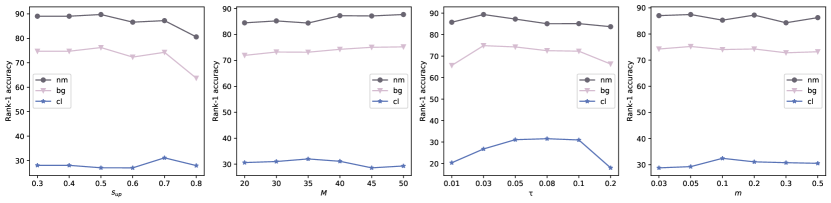
Figure 5: The effect of hyper-parameters $s_{up}/M/\tau/m$ on baselines. In there we choose a set of hyper-paramters that have the best result in our experiments. Other hyper-parameters don’t change the result a lot, just lead to sub-optimal.

4.4.2 Impact of each component in our Selective Fusion

This section, we demonstrate that both SCF and SSF are indispensable in our Selective Fusion method. In Table VI we show the results only using SCF or SSF. Only with SSF, the rank-1 accuracy for each condition in front/back view slightly improved, but still had a poor performance on the cross-cloth problem. When directly applying SCF, clusters mainly composed of sequences in front/back views will also pull closer to other clusters in the same condition, which should be forbidden. Pulling more FVCs closer will further make these sequences harder to merge into their actual clusters with other views, degrading the performance in recognizing sequences with front/back views. Therefore, the best effect can be achieved only when these two methods are effectively combined. Next we will show the effect of parameters used in each method.

TABLE VI: The effectiveness of each components in our framework. Combining both methods can maximum their effect.

Settings	NM	BG	CL
Base	87.2	74.3	31.1
Base + SSF	87.5	75.8	32.8
Base + SCF	83.3	75.9	39.9
Ours	90.3	82.9	40.8

4.4.3 Impact of candidate number in support set

Here we discuss the effect of a parameter in SCF, the candidate number $k$, in support set. In Table VII, we can see that when $k=2$, we have the best performance, which is in line with the fact that the features of NM and BG are easily projected together in the feature space since they have larger similarity and we should drag the features of NM with CL specifically in CASIA-BN.

TABLE VII: The effect of cluster candidates number $k$ in support set.

Settings	NM	BG	CL
Ours ($k=4$)	89.2	81.2	35.1
Ours ($k=3$)	89.7	81.1	37.9
Ours ($k=2$)	90.3	82.9	40.8

4.4.4 Impact of rate of curriculum learning in SSF

We test the effect of SSF with a dynamic or constant rate when conducting curriculum learning. Without curriculum learning, linearly clustering the front/back view sequences with sequences in other views will degrade the performance. With a dynamic pulling rate, we can relax the requirement when training model, which can make the model learn from easy to hard better.

TABLE VIII: The performance of different kinds of rates when conducting curriculum learning.

Settings	NM	BG	CL
Ours ($\lambda_{base}$)	90.3	82.7	40.7
Ours ($\lambda$)	90.3	82.9	40.8

4.4.5 Visulization of Selective Fusion

The visualization effect of Selective Fusion shows in Figure 6.

We select a subject in CASIA-BN, finding that in baseline, BG and CL have a different pseudo label with NM. At the same time, some sequences in front/back views of NM/BG/CL are also assigned with different pseudo labels with sequences in other views. With Selective Fusion, most sequences in various views and different conditions are assigned the same ID.

4.5 Discussion and future work

Our method can be employed with off-the-shelf backbones to train a new unlabeled dataset without a label. However, there are still some limitations.

First, we utilize prior knowledge about the views to identify the challenging samples with front/back views. This is because without such knowledge, it is difficult to specifically group these sequences with other views. More automatic methods can be further developed to reduce the dependence on prior knowledge.

Second, our method uses data augmentation to simulate cross-cloth samples for gait recognition, which makes the model’s recognition performance dependend on the effect of data augmentation to some extent. Therefore, more data augmentation methods can be developed to simulate the real-world cloth changing situations. Also, the intrinsic principles of cross-cloth recognition need further study.

Third, the accuracy of unsupervised learning relies much on the pre-trained model’s accuracy, so a higher precision model is necessary when conducting unsupervised learning on larger datasets, especially on real-world dataset.

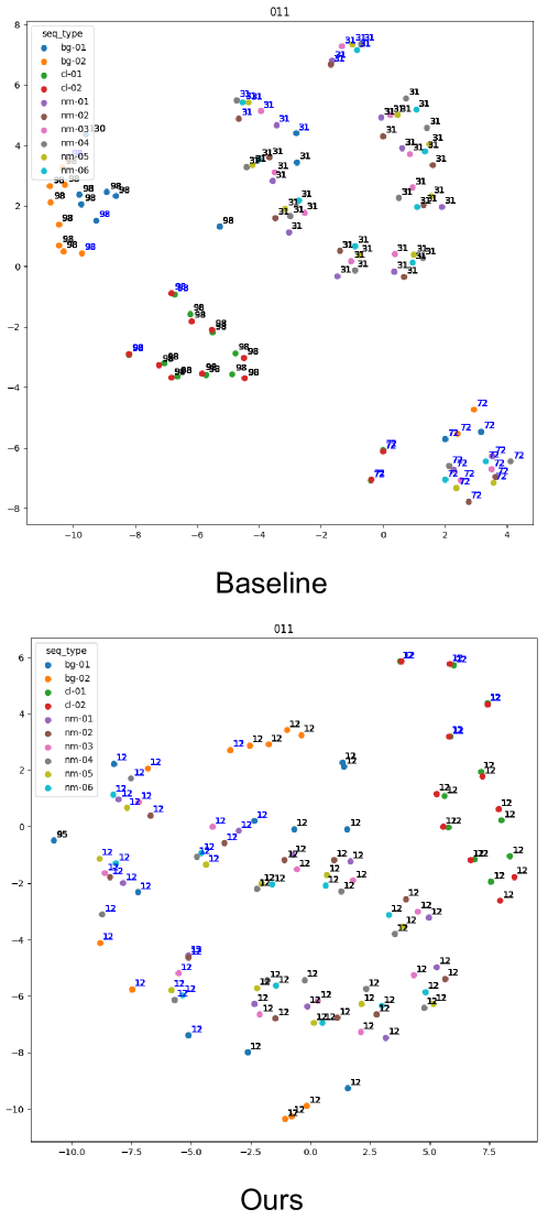
Figure 6: The TSNE images of baseline/Ours. The text above each feature point shows the pseudo label. Blue color in text represents the sequence is in front/back view. A type of color in feature point indicates a type of condition. SF is the Selective Fusion method we proposed. Please scroll in to see the details.

Since OUMVLP is a dataset that captured in the lab environment, it provides limited knowledge when realizing cross-view and cross-cloth on real world data. So further efforts need to be spent on training more robust and high percision pre-train model to make the unsupervised learning method better adapted to real world.

Our work conducts gait recognition with unsupervised learning, which alleviate the human labor requirement in the data collection process, making training gait recognition models with large dataset become possible and economical. This is crucial because currently previous datasets are collected with manual label, which can be a time-consuming and costly process, especially when large datasets are involved. By reducing the amount of human labor required, unsupervised gait recognition make training gait recognition models with large datasets more feasible and cost-effective. Training with larger dataset can ultimately lead to more accurate and robust gait recognition models, which can have a wide range of applications in fields such as security, healthcare, and sports analysis.

In a nutshell, for future work, more intelligent methods can be developed to identify sequences taken from front/back views and and incorporate them with other views correctly. And more robust architecture can be developed to make the gait recognition method stable when adapting to real-world datasets.

5 Conclusion

In this work, we propose a new task, Unsupervised Gait Recognition. We first design a new baseline with cluster-level contrastive learning. Then, we find two problems Unsupervised Gait Recognition faced: sequences in different clothes cannot be gathered into a single cluster, and sequences captured from front/back views are hard to be collected with sequences in other views. To solve the two problems, we propose a Selective Fusion method with Selective Cluster Fusion and Selective Sample Fusion to gradually fuse clusters and sample pairs. Selective Cluster Fusion helps clusters in different clothes of the same person gather as close as possible, and Selective Sample Fusion gradually merges sequences taken from front/back views with sequences in other views. Experiments show the effectiveness and excellent performance in improving the accuracy of CL and front/back view conditions.

6 Biography Section

Xuqian Ren received the B.E. degree from University of Science and Technology Beijing in 2019, received the M.S. degree from Beijing Institute of Technology in 2022. She is currently a Ph.D. candidate with Computer Science Unit, Faculty of Information Technology and Communication Sciences, Tampere Universities, Finland. Her current research interests include contrastive learning, image generation and 3d reconstruction.

Saihui Hou received the B.E. and Ph.D. degrees from University of Science and Technology of China in 2014 and 2019, respectively. He is currently an Assistant Professor with School of Artificial Intelligence, Beijing Normal University, and works in cooperation with Watrix Technology Limited Co. Ltd. His research interests include computer vision and machine learning. He recently focuses on gait recognition which aims to identify different people according to the walking patterns.

Chunshui Cao received the B.E. and Ph.D. degrees from University of Science and Technology of China in 2013 and 2018, respectively. During his Ph.D. study, he joined Center for Research on Intelligent Perception and Computing, National Laboratory of Pattern Recognition, Institute of Automation, Chinese Academy of Sciences. From 2018 to 2020, he worked as a Postdoctoral Fellow with PBC School of Finance, Tsinghua University. He is currently a Research Scientist with Watrix Technology Limited Co. Ltd. His research interests include pattern recognition, computer vision and machine learning.

Xu Liu received the B.E. and Ph.D. degrees from University of Science and Technology of China in 2013 and 2018, respectively. He is currently a Research Scientist with Watrix Technology Limited Co. Ltd. His research interests include gait recognition, object detection and image segmentation.

Yongzhen Huang received the B.E. degree from Huazhong University of Science and Technology in 2006, and the Ph.D. degree from Institute of Automation, Chinese Academy of Sciences in 2011. He is currently an Associate Professor with School of Artificial Intelligence, Beijing Normal University, and works in cooperation with Watrix Technology Limited Co. Ltd. He has published one book and more than 80 papers at international journals and conferences such as TPAMI, IJCV, TIP, TSMCB, TMM, TCSVT, CVPR, ICCV, ECCV, NIPS, AAAI. His research interests include pattern recognition, computer vision and machine learning.

References

- [1] H. Chao, Y. He, J. Zhang, and J. Feng, “Gaitset: Regarding gait as a set for cross-view gait recognition,” in Proceedings of the AAAI conference on artificial intelligence, vol. 33, no. 01, 2019, pp. 8126–8133.
- [2] C. Fan, Y. Peng, C. Cao, X. Liu, S. Hou, J. Chi, Y. Huang, Q. Li, and Z. He, “Gaitpart: Temporal part-based model for gait recognition,” in Proceedings of the IEEE/CVF conference on computer vision and pattern recognition, 2020, pp. 14 225–14 233.
- [3] B. Lin, S. Zhang, and X. Yu, “Gait recognition via effective global-local feature representation and local temporal aggregation,” in Proceedings of the IEEE/CVF International Conference on Computer Vision, 2021, pp. 14 648–14 656.
- [4] S. Yu, D. Tan, and T. Tan, “A framework for evaluating the effect of view angle, clothing and carrying condition on gait recognition,” in 18th international conference on pattern recognition (ICPR’06), vol. 4. IEEE, 2006, pp. 441–444.
- [5] Y. Lin, X. Dong, L. Zheng, Y. Yan, and Y. Yang, “A bottom-up clustering approach to unsupervised person re-identification,” in Proceedings of the AAAI conference on artificial intelligence, vol. 33, no. 01, 2019, pp. 8738–8745.
- [6] Y. Ge, F. Zhu, D. Chen, R. Zhao et al., “Self-paced contrastive learning with hybrid memory for domain adaptive object re-id,” Advances in Neural Information Processing Systems, vol. 33, pp. 11 309–11 321, 2020.
- [7] Y. Lin, L. Xie, Y. Wu, C. Yan, and Q. Tian, “Unsupervised person re-identification via softened similarity learning,” in Proceedings of the IEEE/CVF conference on computer vision and pattern recognition, 2020, pp. 3390–3399.
- [8] D. Wang and S. Zhang, “Unsupervised person re-identification via multi-label classification,” in Proceedings of the IEEE/CVF conference on computer vision and pattern recognition, 2020, pp. 10 981–10 990.
- [9] Z. Dai, G. Wang, W. Yuan, X. Liu, S. Zhu, and P. Tan, “Cluster contrast for unsupervised person re-identification,” arXiv preprint arXiv:2103.11568, 2021.
- [10] K. Nikhal and B. S. Riggan, “Multi-context grouped attention for unsupervised person re-identification,” IEEE Transactions on Biometrics, Behavior, and Identity Science, pp. 1–1, 2022.
- [11] R. Liao, S. Yu, W. An, and Y. Huang, “A model-based gait recognition method with body pose and human prior knowledge,” Pattern recognition, vol. 98, p. 107069, 2020.
- [12] N. Li, X. Zhao, and C. Ma, “Jointsgait: A model-based gait recognition method based on gait graph convolutional networks and joints relationship pyramid mapping,” arXiv preprint arXiv:2005.08625, 2020.
- [13] J. Chen, Z. Wang, P. Yi, K. Zeng, Z. He, and Q. Zou, “Gait pyramid attention network: Toward silhouette semantic relation learning for gait recognition,” IEEE Transactions on Biometrics, Behavior, and Identity Science, vol. 4, no. 4, pp. 582–595, 2022.
- [14] A. Sepas-Moghaddam and A. Etemad, “View-invariant gait recognition with attentive recurrent learning of partial representations,” IEEE Transactions on Biometrics, Behavior, and Identity Science, vol. 3, no. 1, pp. 124–137, 2021.
- [15] X. Huang, X. Wang, B. He, S. He, W. Liu, and B. Feng, “Star: Spatio-temporal augmented relation network for gait recognition,” IEEE Transactions on Biometrics, Behavior, and Identity Science, vol. 5, no. 1, pp. 115–125, 2023.
- [16] R. Wang, Y. Shi, H. Ling, Z. Li, P. Li, B. Liu, H. Zheng, and Q. Wang, “Gait recognition via gait period set,” IEEE Transactions on Biometrics, Behavior, and Identity Science, pp. 1–1, 2023.
- [17] S. Hou, X. Liu, C. Cao, and Y. Huang, “Gait quality aware network: Toward the interpretability of silhouette-based gait recognition,” IEEE Transactions on Neural Networks and Learning Systems, 2022.
- [18] D. Das, A. Agarwal, and P. Chattopadhyay, “Gait recognition from occluded sequences in surveillance sites,” in Computer Vision–ECCV 2022 Workshops: Tel Aviv, Israel, October 23–27, 2022, Proceedings, Part V. Springer, 2023, pp. 703–719.
- [19] S. Zhang, Y. Wang, and A. Li, “Gait energy image-based human attribute recognition using two-branch deep convolutional neural network,” IEEE Transactions on Biometrics, Behavior, and Identity Science, vol. 5, no. 1, pp. 53–63, 2023.
- [20] S. Hou, C. Fan, C. Cao, X. Liu, and Y. Huang, “A comprehensive study on the evaluation of silhouette-based gait recognition,” IEEE Transactions on Biometrics, Behavior, and Identity Science, pp. 1–1, 2022.
- [21] S. Yan, Y. Xiong, and D. Lin, “Spatial temporal graph convolutional networks for skeleton-based action recognition,” in Proceedings of the AAAI conference on artificial intelligence, 2018.
- [22] T. Torben, K. Ali, G. Johannes, H. Fabian, and H. Stefan, “Gaitgraph: Graph convolutional network for skeleton-based gait recognition,” in IEEE International Conference on Image Processing (ICIP). IEEE, 2021, p. 2314–2318.
- [23] K. Zeng, M. Ning, Y. Wang, and Y. Guo, “Hierarchical clustering with hard-batch triplet loss for person re-identification,” in Proceedings of the IEEE/CVF conference on computer vision and pattern recognition, 2020, pp. 13 657–13 665.
- [24] M. Wang, B. Lai, J. Huang, X. Gong, and X.-S. Hua, “Camera-aware proxies for unsupervised person re-identification,” in Proceedings of the AAAI conference on artificial intelligence, vol. 35, no. 4, 2021, pp. 2764–2772.
- [25] H. Chen, B. Lagadec, and F. Bremond, “Ice: Inter-instance contrastive encoding for unsupervised person re-identification,” in Proceedings of the IEEE/CVF International Conference on Computer Vision, 2021, pp. 14 960–14 969.
- [26] S. Xuan and S. Zhang, “Intra-inter camera similarity for unsupervised person re-identification,” in Proceedings of the IEEE/CVF conference on computer vision and pattern recognition, 2021, pp. 11 926–11 935.
- [27] M. Li, P. Xu, X. Zhu, and J. Guo, “Unsupervised long-term person re-identification with clothes change,” arXiv preprint arXiv:2202.03087, 2022.
- [28] Y. Bengio, J. Louradour, R. Collobert, and J. Weston, “Curriculum learning,” in Proceedings of the 26th annual international conference on machine learning, 2009, pp. 41–48.
- [29] N. Takemura, Y. Makihara, D. Muramatsu, T. Echigo, and Y. Yagi, “Multi-view large population gait dataset and its performance evaluation for cross-view gait recognition,” IPSJ Transactions on Computer Vision and Applications, vol. 10, no. 1, pp. 1–14, 2018.
- [30] E. Fix and J. L. Hodges, “Discriminatory analysis. nonparametric discrimination: Consistency properties,” International Statistical Review/Revue Internationale de Statistique, vol. 57, no. 3, pp. 238–247, 1989.
- [31] M. Rosvall and C. T. Bergstrom, “Maps of random walks on complex networks reveal community structure,” Proceedings of the national academy of sciences, vol. 105, no. 4, pp. 1118–1123, 2008.
- [32] C. Song, Y. Huang, Y. Huang, N. Jia, and L. Wang, “Gaitnet: An end-to-end network for gait based human identification,” Pattern recognition, vol. 96, p. 106988, 2019.
- [33] S. Hou, X. Pan, C. C. Loy, Z. Wang, and D. Lin, “Learning a unified classifier incrementally via rebalancing,” in Proceedings of the IEEE/CVF conference on computer vision and pattern recognition, 2019, pp. 831–839.
- [34] A. Paszke, S. Gross, F. Massa, A. Lerer, J. Bradbury, G. Chanan, T. Killeen, Z. Lin, N. Gimelshein, L. Antiga et al., “Pytorch: An imperative style, high-performance deep learning library,” Advances in Neural Information Processing Systems, vol. 32, pp. 8026–8037, 2019.
- [35] K. He, X. Zhang, S. Ren, and J. Sun, “Deep residual learning for image recognition,” in Proceedings of the IEEE/CVF conference on computer vision and pattern recognition, 2016, pp. 770–778.
- [36] J. Deng, W. Dong, R. Socher, L.-J. Li, K. Li, and L. Fei-Fei, “Imagenet: A large-scale hierarchical image database,” in Proceedings of the IEEE/CVF conference on computer vision and pattern recognition. Ieee, 2009, pp. 248–255.
- [37] C. Fan, J. Liang, C. Shen, S. Hou, Y. Huang, and S. Yu, “Opengait: Revisiting gait recognition toward better practicality,” arXiv preprint arXiv:2211.06597, 2022.