Dictionary-based model reduction for state estimation

Abstract

We consider the problem of state estimation from $m$ linear measurements, where the state $u$ to recover is an element of the manifold $\mathcal{M}$ of solutions of a parameter-dependent equation. The state is estimated using a prior knowledge on $\mathcal{M}$ coming from model order reduction. Variational approaches based on linear approximation of $\mathcal{M}$, such as PBDW, yields a recovery error limited by the Kolmogorov $m$-width of $\mathcal{M}$. To overcome this issue, piecewise-affine approximations of $\mathcal{M}$ have also be considered, that consist in using a library of linear spaces among which one is selected by minimizing some distance to $\mathcal{M}$. In this paper, we propose a state estimation method relying on dictionary-based model reduction, where a space is selected from a library generated by a dictionary of snapshots, using a distance to the manifold. The selection is performed among a set of candidate spaces obtained from the path of a $\ell_{1}$-regularized least-squares problem. Then, in the framework of parameter-dependent operator equations (or PDEs) with affine parameterizations, we provide an efficient offline-online decomposition based on randomized linear algebra, that ensures efficient and stable computations while preserving theoretical guarantees.

Keywords.

inverse problem, model order reduction, sparse approximation, randomized linear algebra.

MSC Classification.

65M32, 62J07, 60B20,

1 Introduction

This paper is concerned with state estimation (or inverse) problems that consist in the approximation (or recovery) of an element $u$ of a Hilbert space $U$ using linear measurements and the additional knowledge that $u$ is the solution of a parameter-dependent equation

$$\mathcal{F}\big{(}u(\xi),\xi\big{)}=0,$$ (1)

for some unknown parameter $\xi$ in a parameter set $\mathcal{P}$. In other words, the sought state $u$ is an element of the so called solution manifold

$$\mathcal{M}:=\{u(\xi):\xi\in\mathcal{P}\}\subset U,$$ (2)

and we aim to approximate $u$ by using $m$ measurements $\ell_{1}(u)$, …, $\ell_{m}(u)$, where the $\ell_{i}$ are continuous linear forms on $U$, along with some prior knowledge on $\mathcal{M}$ coming from model order reduction (MOR).

A variational approach called parameterized-background data-weak (PBDW) was proposed in [21]. It relies on the assumption that $\mathcal{M}$ can be well approximated by a low-dimensional linear space $V$, which can be obtained by, e.g., principal component analysis or greedy algorithms. The PBDW state estimate is then obtained as the sum of an element from the background space $V$ and a correction in the observation space $W$ generated by the Riesz representers of the linear forms $\ell_{i}$. However, the background space and the measurements should be compatible for ensuring stability of the estimation, especially in the case of noisy observations [22]. More precisely, stability is related to the alignment of spaces $V$ and $W$. There are two main approaches to overcome this issue. The first is to select carefully an observation space that is adapted to the given space $V$, e.g., by selecting the linear forms from a dictionary using a greedy algorithm [6]. In practice, this approach may not perform well if the number and type of measurements (e.g., location of sensors) are restricted. The second approach is to consider a different prior knowledge for $\mathcal{M}$, by constructing a space $V$ adapted to the measurements, e.g., using the optimization procedure from [10], or by taking advantage of a wider knowledge coming from the construction of $V$ by a greedy algorithm, as proposed in [5, 17]. In the case of noisy observations, the authors in [26] propose a regularized version of PBDW, that consists in considering elements from a bounded subset of the background space $V$.

The above approaches are all based on linear approximation, which may poorly perform in cases where the manifold $\mathcal{M}$ can not be well approximated by a single linear space of small dimension, that is characterized by a slow decay of its Kolmogorov $n$-width

$$d_{n}(\mathcal{M})_{U}:=\inf_{\text{dim}V=n}\sup_{u\in\mathcal{M}}\min_{v\in V}\|u-v\|_{U},$$ (3)

which is the best worst-case error we can expect when approximating $\mathcal{M}$ by a $n$-dimensional subspace $V$ in $U$.

Hence, there are incentives to consider non-linear approximations of $\mathcal{M}$, like the piecewise-affine approximation proposed in [11], which relies on a library of subspaces among which one space is selected by minimizing some distance to the manifold, or the approach based on manifold approximation [12].

1.1 Contributions and outline

Our first contribution is a state estimation strategy using dictionary-based reduced order models [4, 18]. It consists in using a library of background low-dimensional spaces generated by a large dictionary $\mathcal{D}_{K}$ of $K$ snapshots in $\mathcal{M}$. Our approach is an adaptation of the approach from [11] to a setting where we have access to a combinatorial number $\binom{K}{n}$ of candidate background spaces of low dimension $n$. A benchmark error for this model order reduction method is the nonlinear Kolmogorov width from [27] defined by

$$d_{n}(\mathcal{M},N)_{U}:=\inf_{\#\mathcal{L}_{n}^{N}=N}\sup_{u\in\mathcal{M}}\min_{V\in\mathcal{L}_{n}^{N}}\min_{v\in V}\|u-v\|_{U},$$ (4)

where the infimum is taken over all libraries $\mathcal{L}_{n}^{N}$ of $N$ subspaces of dimension $n$, with $N=\binom{K}{n}$, that is $N\sim K^{n}$ in the regime $K\gg n.$ With this dictionary-based approach, it is expected to select a low-dimensional background space among a huge candidate set, yielding a good approximation of $\mathcal{M}$ and a good stability of the estimation problem in the case where only a few measurements are available.

Our second contribution is to provide an efficient offline-online decomposition for our dictionary-based approach, in the framework of parameter-dependent operator equations (or PDEs) with affine parametrization. Indeed, classical offline precomputations for residual-based quantities often lead to prohibitive offline costs when it comes to dictionary-based approaches, as pointed out in [18, 4]. They also tend to be sensible to round-off errors. For solving these issues, and following [2], we rely on randomized linear algebra (RLA), that allows for efficient and stable computations, with theoretical guarantees.

The outline is as follows. First in Section 2 we recall the original PBDW approach from [21], which was called the one-space problem in [5]. We also recall the error bounds for this approach, as well as its limitations.

Then in Section 3 we describe a general multi-space problem, in which the background space $V$ is selected adaptively among a library $\mathcal{L}_{n}^{N}$ containing $N$ subspaces of dimension at most $n$. The space is selected using a surrogate distance $\mathcal{S}$ to the manifold $\mathcal{M}$ and the associated recovery error is controlled, under certain assumptions, by the best recovery error among $\mathcal{L}_{n}^{N}$. This approach was introduced in [11] for a specific choice of library. Here, it is presented in a general setting.

In Section 4, we present a randomized version of the selection method for the general multi-space problem, based on RLA techniques for the estimation of $\mathcal{S}$. We prove that our randomized approach provides a priori error bounds similar to the non-randomized approach with high (user-defined) probability. This approach makes feasible an offline-online decomposition, with reasonable offline costs, low online costs and robustness to round-off errors. These computational aspects are developed in the next section.

In Section 5, we consider a dictionary-based multi-space problem, in which the library contains all the subspaces generated by $n$ elements of some dictionary $\mathcal{D}_{K}$ of size $K$. More precisely, for computational reasons, we use adaptive libraries obtained from the path of solutions of $\ell_{1}$-regularized optimization problems. In the framework of parametric operator equations (or PDEs), the randomized selection from the previous section allow us to select efficiently a good subspace among those generated, with an associated error controlled by the best error among the adaptive library.

Finally in Section 6 we test our approach on two different numerical examples. First a classical thermal-block diffusion problem, then an advection-diffusion problem.

1.2 Setting and notations

Instead of referring to the measurements $\ell_{1}(u)$, …, $\ell_{m}(u)$, we will equivalently consider the orthogonal projection $w=P_{W}u$ of the state $u$ onto the observation space

$$W:=\text{span}\{R_{U}^{-1}\ell_{i}:1\leq i\leq m\}\subset U,$$ (5)

where $R_{U}:U\rightarrow U^{\prime}$ is the Riesz map. We assume (w.l.o.g.) that the linear forms are linearly independent, which implies that the space $W$ is of dimension $m$. The problem of state estimation is equivalent to finding a recovery map $A:W\to U$ which associates to an observation $w\in W$ an element $A(w)\in U$.

Our methodology is valid for real or complex Hilbert spaces, but for the sake of simplicity, we restrict the presentation to the real case. In practice, although most of our results are valid for a general Hilbert setting, the space $U$ is of finite dimension $\mathcal{N}$. In the context of PDEs, the space arises from some discretization (e.g., based on finite elements, finite volumes…) and its dimension $\mathcal{N}$ is usually very large to ensure high fidelity towards the true solution. The space $U$ and its dual $U^{\prime}$ are then identified with $\mathbb{R}^{\mathcal{N}}$, respectively endowed with inner products $\langle\cdot,\cdot\rangle_{U}=\langle\cdot,\mathbf{R}_{\mathrm{U}}\cdot\rangle_{\ell_{2}}$ and $\langle\cdot,\cdot\rangle_{U^{\prime}}=\langle\cdot,\mathbf{R}_{\mathrm{U}}^{-1}\cdot\rangle_{\ell_{2}}$, where $\langle\cdot,\cdot\rangle$ denotes the canonical $\ell_{2}$-inner product in $\mathbb{R}^{\mathcal{N}}$, and where $\mathbf{R}_{\mathrm{U}}\in\mathbb{R}^{\mathcal{N}\times\mathcal{N}}$ is the positive definite symmetric matrix associated with the Riesz map $R_{U}$. Discrete representations of operators and vectors will be systematically written with bold notations.

2 The one-space problem, or PBDW

The one-space problem was initially called Parameterized-Background Data Weak (PBDW) and formulated in [21]. We denote by $A_{V}:W\rightarrow W+V$ the corresponding recovery map for some background space $V$. In this section, we consider that the only knowledge we have on $\mathcal{M}$ is that it is well approximated by a $n$-dimensional space $V_{n}$, with

$$\text{dist}(V_{n},\mathcal{M})=\sup_{u\in\mathcal{M}}\min_{v\in V_{n}}\|u-v\|\leq\varepsilon_{n}.$$

Note that for the one-space problem, the precision $\varepsilon_{n}$ is not required to be known to compute the state estimate, while it is the case in the nested multi-space problem in Section 3.1.

2.1 Variational formulation

The PBDW problem was first formulated as a variational problem. For an observation $w=P_{W}u$, the recovery $A_{V_{n}}(w)$ is obtained by selecting the background term $v^{*}\in V_{n}$ which requires the smallest update $\eta^{*}\in W$. In other words,

$$A_{V_{n}}(w):=v^{*}+\eta^{*}\quad\text{with}\quad\left\{\begin{aligned} &v^{*}:=\arg\min_{v\in V_{n}}\|P_{W}(u-v)\|_{U}\\ &\eta^{*}:=P_{W}(u-v^{*})\end{aligned}\right..$$ (6)

In a finite dimensional setting, with $U=\mathbb{R}^{\mathcal{N}}$, the problem (6) has the following algebraic form:

$$A_{V_{n}}(w):=v^{*}+\eta^{*}\quad\text{with}\quad\left\{\begin{aligned} &v^{*}=\mathbf{V}\mathbf{v}^{*},\quad\mathbf{v}^{*}:=\arg\min_{\mathbf{v}\in\mathbb{R}^{n}}\|\mathbf{C}\mathbf{v}-\mathbf{w}\|_{2},&\\ &\eta^{*}=\mathbf{W}\boldsymbol{\eta}^{*},\quad\boldsymbol{\eta}^{*}:=\mathbf{w}-\mathbf{C}\mathbf{v}^{*},&\end{aligned}\right.$$ (7)

where $\mathbf{V}\in\mathbb{R}^{\mathcal{N}\times n}$ and $\mathbf{W}\in\mathbb{R}^{\mathcal{N}\times m}$ are the matrices whose columns form an orthonormal basis of $V_{n}$ and $W$ respectively, $\mathbf{C=W^{\mathsf{T}}\mathbf{R}_{\mathrm{U}}V}\in\mathbb{R}^{m\times n}$ is the cross gramian-matrix, and $\mathbf{w}\in\mathbb{R}^{m}$ is such that $w=\mathbf{Ww}$. Problem (6) is well-posed if and only if $V_{n}~{}\cap~{}W^{\perp}=\{0\}$. This is equivalent to $\sigma_{\text{min}}(\mathbf{C})>0$ with $n\leq m$. For the PBDW estimation, we assume that this condition is satisfied. The analysis from [5] then ensures the error bound

$$\|u-A_{V_{n}}(w)\|_{U}\leq\mu(V_{n},W)\varepsilon_{n},$$ (8)

where $\mu(V_{n},W)$ is the inverse of the smallest singular value $\beta(V_{n},W)$ of the projection operator $P_{W}$ restricted to $V_{n}$. These constants are defined by

$$\begin{aligned} \mu(V_{n},W)&:=\sup_{\eta\in W^{\perp}}\frac{\|\eta\|_{U}}{\|\eta-P_{V_{n}}\eta\|_{U}}=\sigma_{\text{min}}(\mathbf{C})^{-1},\\ \beta(V_{n},W)&:=\inf_{v\in V_{n}}\frac{\|P_{W}v\|_{U}}{\|v\|_{U}}=\inf_{v\in V_{n}}\sup_{w\in W}\frac{\langle v,w\rangle_{U}}{\|v\|_{U}\|w\|_{U}}=\sigma_{\text{min}}(\mathbf{C}).\end{aligned}$$ (9)

2.2 Geometric formulation and optimality

The geometric interpretation of the problem described in Section 2.1 was provided and analysed in [5]. In the one-space problem, the manifold can be considered as the cylinder $\mathcal{K}^{n}$ defined by

$$\mathcal{K}^{n}:=\{v\in U:\text{dist}(v,V_{n})\leq\varepsilon_{n}\}.$$ (10)

Given an observation $w=P_{W}u$, all the knowledge we have about $u$ is that $u\in\mathcal{K}^{n}_{w}$, where

$$\mathcal{K}^{n}_{w}:=\mathcal{K}^{n}\cap U_{w},\quad U_{w}:=w+W^{\perp}.$$ (11)

The optimal recovery map, in the sense of the worst case error in $\mathcal{K}^{n}$, is the one mapping $w$ to the Chebyshev center of $\mathcal{K}^{n}_{w}$, where the Chebyshev center is defined for any bounded set $\mathcal{X}\subset U$ by

$$\text{cen}(\mathcal{X}):=\mathop{\mathrm{argmin}}_{v\in U}\inf\{r:\mathcal{X}\subset\overline{\mathcal{B}(v,r)}\},$$ (12)

which is well defined and unique. It has been shown that $A_{V_{n}}$ is the optimal map when the manifold is the cylinder $\mathcal{K}^{n}$. In other words $A_{V_{n}}(w)=\text{cen}(\mathcal{K}^{n}_{w})$ and

$$A_{V_{n}}=\min_{A:W\rightarrow U}\sup_{u\in\mathcal{K}^{n}}\|u-A(P_{W}u)\|_{U},$$ (13)

where the minimum is taken over all linear maps from $W$ to $U$. In Figure 1 we illustrate this geometric formulation.

(a)

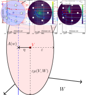
(b)

Figure 1: Geometric interpretation of the PBDW recovery for one observation $w=P_{W}u$, with dim$(W)=2$ and dim$(V)=1$.

The one-space problem may have bad performances when the background space $V_{n}$ is not well aligned with the observation space $W$, which leads to a bad $\mu(V_{n},W)$, or when the manifold cannot be well approximated by a single linear space, which leads to a bad $\varepsilon_{n}$. The approximation by a single subspace is inherently limited by the Kolmogorov $m$-width via the bound $\varepsilon_{n}\geq d_{m}(\mathcal{M})_{U}$ because $n\leq m$.

3 The multi-space problem

Several approaches have been proposed for addressing the issues of the one-space approach [10, 17, 11]. These are multi-space approaches that consist in exploiting a library of $N$ spaces $V_{1}$, …, $V_{N}$.

First in Section 3.1 we present the multi-space approach as first described in [5]. Then in Section 3.2 we present the multi-space approach proposed in [11], with a selection method based on some surrogate distance to the manifold, and recall the associated oracle error bound which holds not only in the piecewise-affine framework considered in [11]. This piecewise affine framework is considered in Section 3.3. Finally in Section 3.4, we focus on the case where problem (1) is a parameter-dependent PDE, which provides (under suitable conditions) a natural residual-based surrogate distance.

3.1 Nested multi-space

The library corresponding to the multi-space approach from [5] is constituted of a nested sequence of subspaces with increasing approximation powers. In this subsection, we consider a library composed of $N=n\leq m$ nested subspaces such that

$$V_{1}\subset\cdots\subset V_{n},\quad\text{dim}(V_{j})=j,\quad\text{dist}(\mathcal{M},V_{j})\leq\varepsilon_{j},\quad 1\leq j\leq n.$$

For an observation $w\in W$ we consider the compact set

$$\mathcal{K}^{\text{mult}}_{w}:=U_{w}\cap\mathcal{K}^{\text{mult}},\quad\mathcal{K}^{\text{mult}}:=\bigcap_{j=1}^{n}\mathcal{K}^{j},\quad U_{w}:=w+W^{\perp}.$$ (14)

where the cylinders $\mathcal{K}^{j}$ for $1\leq j\leq n$ are defined by (10), as for the one-space problem. The optimal recovery map for the worst case error would be the map $w\mapsto\text{cen}(\mathcal{K}^{\text{mult}}_{w})$. However, contrary to the one-space problem, this optimal map is not computable in general. In [5], the authors propose to select any map $A^{\text{mult}}$ such that

$$A^{\text{mult}}(w)\in\mathcal{K}^{\text{mult}}_{w}.$$ (15)

They showed that any map satisfying (15) satisfies the oracle error bound

$$\sup_{u\in\mathcal{K}^{\text{mult}}}\|u-A^{\text{mult}}(P_{W}u)\|\leq\sqrt{2}\min_{1\leq j\leq n}\mu(V_{j},W)\varepsilon_{j}.$$ (16)

They also propose numerical algorithms to compute such a map. It is important to note that the proposed algorithms require to know the widths $(\varepsilon_{j})_{1\leq j\leq n}$ to be performed, whereas it is not the case for the one-space problem. This approach allows to take advantage of the best compromise possible between $\varepsilon_{j}$ and $\mu(V_{j},W)$ among all the available spaces. However it is not well adapted to problems with slow decay of Kolmogorov $n$-width, similarly as the one-space problem.

We end this subsection by citing the works from [17] which also consider the nested multi-space framework. The authors propose a recovery map $A$ such that $A(w)\in V_{n}\cap\mathcal{K}^{\text{mult}}$ minimizes the norm of the update term $w-P_{W}A(w)$ . Note that [17] also extends the multi-space problem to the case $m<n$ and provides error bounds, ensuring stability when increasing the knowledge with $n-m$ new spaces with better approximation power, although the error bounds provided are not sharp. We also cite the works from [10] in which the background space is obtained via a convex optimization problem.

3.2 General approach

The general multi-space approach consists in using not a single space $V_{n}$ as background, as for the initial PBDW approach, but rather a library

$$\mathcal{L}_{n}^{N}:=\{V_{1},\cdots,V_{N}\}$$

of $N$ subspaces of dimension at most $n$. We suppose that

$$n_{k}:=\text{dim}(V_{k})\leq n\leq m,\hskip 14.22636pt1\leq k\leq N.$$

The benchmark error for this non-linear model order reduction method is the library-based non linear Kolmogorov $n$-width from [27] defined by (4). For some $N=N(n)$, the library width $d_{n}(\mathcal{M},N(n))_{U}$ may have a (much) faster decay with $n$ than $d_{n}(\mathcal{M})_{U}$, so that a small error may be obtained with spaces of low dimension $n$, which can be crucial for our state estimation problem. To each subspace is associated the one-space recovery map

$$A_{k}:=A_{V_{k}}.$$ (17)

For a given observation $w$, it was proposed in [11] to select one of those maps by minimizing some surrogate distance to the manifold $\mathcal{S}(\cdot,\mathcal{M})$. The idea is to select $k^{*}=k^{*}_{\mathcal{S}}(w)$ whose associated one-space recovery is the closest to the manifold, in the sense that it minimizes $\mathcal{S}(\cdot,\mathcal{M})$. This recovery is then denoted as $A^{\text{mult}}_{\mathcal{S}}(w)$. In other words,

$$A^{\text{mult}}_{\mathcal{S}}(w):=A_{k^{*}}(w)\quad\text{with}\quad k^{*}\in\mathop{\mathrm{argmin}}_{1\leq k\leq N}~{}\mathcal{S}(A_{k}(w),\mathcal{M}).$$ (18)

The best choice for $\mathcal{S}$ would be the distance based on the $\|\cdot\|_{U}$ norm. However, this approach may not be computationally feasible in most practical cases where $\mathcal{N}$ is large and elements in $\mathcal{M}$ are expensive to compute or store. Still, assuming that $\mathcal{S}(\cdot,\mathcal{M})$ controls the true distance to $\mathcal{M}$, interesting bounds can be shown. Let us assume that there exist constants $0<c\leq C<+\infty$ such that

$$c~{}\text{dist}(v,\mathcal{M})\leq\mathcal{S}(v,\mathcal{M})\leq C~{}\text{dist}(v,\mathcal{M}).$$ (19)

Then in [11, Theorem 3.4], the authors manage to control the error of the selected estimate by the best recovery error among the library. Although they work with a library built by a piecewise affine model reduction approach, their result still holds for a general library. They introduce and analyse the constant $\mu(\mathcal{M},W)$ defined by

$$\mu(\mathcal{M},W):=\frac{1}{2}\sup_{\sigma>0}\frac{\delta_{\sigma}-\delta_{0}}{\sigma}$$ (20a)

with

$$\delta_{\sigma}:=\max_{w\in W}\text{diam}(\mathcal{M}_{\sigma}\cap U_{w})\quad\text{and}\quad\mathcal{M}_{\sigma}:=\big{\{}v\in U:\text{dist}(v,\mathcal{M})\leq\sigma\big{\}},$$ (20b)

where $\mathcal{M}_{\sigma}$ is the $\sigma$-fattening of $\mathcal{M}$. The constant $\mu(\mathcal{M},W)$ reflects the stability of the recovery problem, independently on the method used for the approximation of $\mathcal{M}$. In other words, it reflects how well $\mathcal{M}$ and $W$ are aligned. The preferable case is when $\delta_{0}=0$. It is equivalent to $P_{W}$ being injective on $\mathcal{M}$. In this case, the error on $A_{\mathcal{S}}^{\text{mult}}$ is truly controlled by the best possible error within the library, as shown in Proposition 1.

Proposition 1.

Assume that $\mu(\mathcal{M},W)<\infty$, then for all $u\in\mathcal{M}$,

$$\|u-A^{\text{mult}}_{\mathcal{S}}(P_{W}u)\|_{U}\leq\delta_{0}+2\kappa\mu(\mathcal{M},W)\min_{1\leq k\leq N}\|u-A_{k}(P_{W}u)\|_{U},$$ (21)

where $\kappa:=\frac{C}{c}$.

Proof.

Let us pick the $k_{\text{best}}$-th subspace from $\mathcal{L}_{n}^{N}$ as the space associated to the best one-space recovery,

$$k_{\text{best}}=\mathop{\mathrm{argmin}}_{1\leq k\leq N}\|u-A_{k}(w)\|_{U}.$$

Using (19) and the definition of $k^{*}$ from (18), it follows that

$$\text{dist}(A_{k^{*}}(w),\mathcal{M})\leq\frac{1}{c}\mathcal{S}(A_{k^{*}}(w),\mathcal{M})\leq\frac{1}{c}\mathcal{S}(A_{k_{\text{best}}}(w),\mathcal{M})\leq\frac{C}{c}\text{dist}(A_{k_{\text{best}}}(w),\mathcal{M}),$$

that is

$$\text{dist}(A_{k^{*}}(w),\mathcal{M})\leq\kappa\lambda,\quad\text{with}\quad\lambda:=\text{dist}(A_{k_{\text{best}}}(w),\mathcal{M}).$$

Hence, since $A_{k^{*}}(w)\in U_{w}$ by definition (6), $A_{k^{*}}(w)\in\mathcal{M}_{\kappa\lambda}\cap U_{w}$. Since $u$ also lies in this set, the recovery error using $A^{\textup{mult}}_{\mathcal{S}}=A_{k^{*}}$ is bounded via

$$\|u-A^{\textup{mult}}_{\mathcal{S}}(w)\|_{U}\leq\text{diam}(\mathcal{M}_{\kappa\lambda}\cap U_{w})\leq\delta_{\kappa\lambda}.$$

We now distinguish the cases $\lambda=0$ and $\lambda>0$. If $\lambda=0$, we have $\|u-A^{\textup{mult}}_{\mathcal{S}}(w)\|_{U}\leq\delta_{0}$, which implies (21). If $\lambda>0$, using

$$\delta_{\kappa\lambda}\leq\delta_{0}+2\kappa\lambda\mu(\mathcal{M},W),$$

and $\lambda\leq\|u-A_{k_{\text{best}}}(w)\|_{U}$ (since $u\in\mathcal{M}$), we also obtain (21). ∎

This general library-based approach allows to perform one-space recovery in background spaces of low dimension, hence potentially good $\mu(V_{k^{*}},W)$, while ensuring good approximation power of the selected background space. However, as stated in [4], some problems require a very large number $N$ of spaces to ensure good precisions $(\varepsilon_{k})_{1\leq k\leq N}$. Hence testing each of the recovery maps $A_{k}$ for every new observation $w\in W$ can be a computational burden online. Our dictionary-based approach described in Section 5, as well as our random sketching approach in Section 4.2, aim to circumvent this issue.

3.3 Piecewise multi-space

This subsection is consecrated to the case where the spaces in the library are obtained via partitioning of the parameter space $\mathcal{P}$ and the manifold $\mathcal{M}$, such that

$$\mathcal{P}=\bigcup_{k=1}^{N}\mathcal{P}^{(k)},\hskip 14.22636pt\mathcal{M}=\bigcup_{k=1}^{N}\mathcal{M}^{(k)},\hskip 14.22636pt\mathcal{M}^{(k)}=\{u(\xi):\xi\in\mathcal{P}^{(k)}\}.$$ (22)

The piecewise multi-space approach then consists in building $N$ spaces with moderate dimension, where the space $V_{k}$ approximates the piece $\mathcal{M}^{(k)}$. The so called hp-refinement methods, as in [15, 14], are examples of such nonlinear methods for model order reduction. Recovery algorithms using such reduced spaces were considered in [11], and it was the initial framework for the general approach described in Section 3.2. They also covered the case of a library of affine spaces, but we do not extend on it in the present paper. In this subsection, we consider a library

$$\mathcal{L}_{n}^{N}=\{V_{k}:1\leq k\leq N\}\quad\text{with}\quad\text{dim}(V_{k})=n_{k}\leq n\leq m,$$

with the one-space constants associated to each sub-manifold,

$$\begin{gathered}\varepsilon_{k}:=\text{dist}(\mathcal{M}^{(k)},V_{k}),\quad\mu_{k}:=\mu(V_{k},W),\quad 1\leq k\leq N.\end{gathered}$$

In this framework, using the general approach described in Section 3.2, it is possible to ensure error bounds depending on the quantity $\mathcal{S}$ used for model selection. If $\mathcal{S}$ satisfies equation (19), then for $\sigma:=\max_{1\leq k\leq N}\varepsilon_{k}\mu_{k}$ we have the error bound [11, Theorem 3.2]

$$\|u-A^{\text{mult}}_{\mathcal{S}}(P_{W}u)\|_{U}\leq\delta_{\kappa\sigma},$$ (23)

with $\delta_{\kappa\sigma}$ defined in (20). This piecewise multi-space approach may suffer from computational problems when the required number $N$ of subspaces becomes too large to satisfy a desired precision. Moreover, it is sensitive to the parametrization of the initial problem (1), hence it may require some preliminary reformulation of the problem before the generation of background spaces. Both of those issues may be circumvented by the dictionary-based approach proposed in Section 5.

3.4 Parameter-dependent operator equations

In this subsection we assume that the parametric problem (1) is actually a parameter-dependent operator equation (or PDE)

$$B(\xi)u(\xi)=f(\xi)$$ (24)

where $B(\xi):U\to U^{\prime}$ is the operator and $f(\xi)\in U^{\prime}$ the right-hand side. In this framework, it is common to consider a residual-based error as a surrogate to the error in the norm $\|\cdot\|_{U}$. We define for all $v\in U$,

$$\mathcal{S}(v,\mathcal{M})=\min_{\xi\in\mathcal{P}}\mathcal{R}(v,\xi),\quad$$ (25a)

with

$$\mathcal{R}(v,\xi):=\|r(v,\xi)\|_{U^{\prime}},\quad r(v,\xi):=B(\xi)v-f(\xi)\in U^{\prime},\quad\forall\xi\in\mathcal{P}.$$ (25b)

For the quantity $\mathcal{S}$ to be equivalent to the error $\|u-v\|_{U}$, and in order to derive error bounds, some assumptions are required on the operator $B(\xi)$. In the case where $B(\xi)$ is linear, we assume that its singular values are uniformly bounded in $\xi$, that is

$$0<c\leq\min_{v\in U}\frac{\|B(\xi)v\|_{U^{\prime}}}{\|v\|_{U}}\leq\max_{v\in U}\frac{\|B(\xi)v\|_{U^{\prime}}}{\|v\|_{U}}\leq C<\infty,$$ (26)

for all $\xi\in\mathcal{P}$, for some constants $c$ and $C$. This implies that for all $v\in U$,

$$c\|v-u(\xi)\|_{U}\leq\mathcal{R}(v,\xi)\leq C\|v-u(\xi)\|_{U},\quad\forall\xi\in\mathcal{P},$$ (27a)

and

$$c~{}\text{dist}(v,\mathcal{M})\leq\mathcal{S}(v,\mathcal{M})\leq C~{}\text{dist}(v,\mathcal{M}).$$ (27b)

Moreover, under additional assumptions on $B$ and $f$, it is possible to compute $\mathcal{R}(v,\cdot)$ in an online efficient way, i.e. with costs independent on $\mathcal{N}$, by taking advantage of the fact that $v$ lies in a low-dimensional subspace. Furthermore, computing $\mathcal{S}$ does not require to know any element in $\mathcal{M}$, whereas the true distance does. We provide a more detailed discussion on the computational aspects in Section 5.4.

Remark 1.

In [11] the authors proposed another residual-based nonlinear recovery map, which is

$$A(w)=\mathop{\mathrm{argmin}}_{v\in w+W^{\perp}}\min_{\xi\in\mathcal{P}}\mathcal{R}(v,\xi),$$

which yields an error $\|A(w)-u\|_{U}\leq\delta_{0}$ in our noiseless setting. In some cases, as when $B(\xi)$ is linear and $\xi\mapsto B(\xi)$ and $\xi\mapsto f(\xi)$ are affine functions of $\xi$, the function $(v,\xi)\mapsto\mathcal{R}(v,\xi)^{2}$ is convex and quadratic in each component, hence the previous problem can be tackled with an alternating minimization procedure. Numerical experiments showed very good results for large enough number of measurements $m$. However, it requires solving online about $m$ high dimensional problems, which is prohibitive for large $\mathcal{N}$.

Remark 2.

The properties (27) also hold in the case of a Lipschitz continuous and strongly monotone nonlinear operator $B(\xi)$, where $c$ is a uniform lower bound of the strong monotonicity constant and $C$ is a uniform bound of the Lipschitz constant. However, in a nonlinear setting, additional efforts are required for obtaining efficient online and offline computations.

Remark 3.

A preconditioned residual could be used to obtain a better condition number $\kappa$. Using preconditioners to better estimate the $U$-norm in a model order reduction setting was proposed in [31, 3].

4 Randomized multi-space approach

First in Section 4.1 we recall some required preliminaries on randomized linear algebra. Then in Section 4.2, we propose to use a sketched (or randomized) version of the selected criterion from Section 3.4 in the framework of parameter-dependent operator equations. We show that, with a rather small sketch and high probability, an oracle bound similar to the non-sketched approach holds.

4.1 Randomized linear algebra

A basic task of RLA is to approximate norms and inner products of high dimensional vectors, by operating on lower dimensional vectors obtained through a random embedding or random sketching. Such embedding does not only reduce the computational time for evaluating norms and inner products, but also reduce the memory consumption since only the embedded vectors need to be stored.

We first recall the notion of $U\rightarrow\ell_{2}$ embedding for a subspace $Y\subset U$, which is a generalisation from [2] of the notion of $\ell_{2}$ embedding for a subspace introduced in [30]. Let $\mathbf{\Theta}\in\mathbb{R}^{k\times\mathcal{\mathcal{N}}}$ be a random matrix, where $k$ is the embedding dimension, that represents a linear map $\Theta$ from $(U,\langle\cdot,\cdot\rangle_{U})$ to $(\mathbb{R}^{k},\langle\cdot,\cdot\rangle)$ $U$ to $\ell_{2}$. This map allows to define (sketched) semi-inner products

$$\langle\cdot,\cdot\rangle_{U}^{\Theta}=\langle\mathbf{\Theta}\cdot,\mathbf{\Theta}\cdot\rangle\hskip 14.22636pt\text{and}\hskip 14.22636pt\langle\cdot,\cdot\rangle_{U^{\prime}}^{\Theta}=\langle\mathbf{\Theta}\mathbf{R}_{\mathrm{U}}^{-1}\cdot,\mathbf{\Theta}\mathbf{R}_{\mathrm{U}}^{-1}\cdot\rangle,$$ (28)

and associated semi-norms $\|\cdot\|_{U}^{\Theta}$ and $\|\cdot\|_{U^{\prime}}^{\Theta}$ respectively. We now define formally the notion of subspace embedding.

Definition 1.

$\mathbf{\Theta}$ is called a $U\rightarrow\ell_{2}$ $\epsilon$-subspace embedding for $Y$, with $\epsilon\in[0,1)$, if

$$\Big{|}\|v\|_{U}^{2}-\|v\|_{U}^{\Theta~{}2}\Big{|}\leq\epsilon\|v\|_{U}^{2},\quad\forall v\in Y.$$ (29)

It can be shown that if $\mathbf{\Theta}$ is a $U\rightarrow\ell_{2}$ $\epsilon$-subspace embedding for $Y$ then $\mathbf{\Theta}\mathbf{R}_{\mathrm{U}}^{-1}$ is a $U^{\prime}\rightarrow\ell_{2}$ $\epsilon$-subspace embedding for $Y^{\prime}$. Hence, both $\|\cdot\|_{U}$ and $\|\cdot\|_{U^{\prime}}$ are well approximated by their sketched versions.

This definition is a property of $\mathbf{\mathbf{\Theta}}$ for a specific subspace $Y$. We are interested in the probability of failure for the random embedding $\mathbf{\Theta}$ to be a $U\rightarrow\ell_{2}$ $\epsilon$-subspace embedding for any $d$-dimensional subspace $Y$ of $U$. With this in mind, the notion of oblivious embedding is defined.

Definition 2.

$\mathbf{\Theta}$ is called a $(\epsilon,\delta,d)$ oblivious $U\rightarrow\ell_{2}$ subspace embedding if for any $d$-dimensional subspace $Y$ of $U$,

$$\mathbb{P}(\mathbf{\Theta}\text{ is a }U\rightarrow\ell_{2}~{}\epsilon\text{-subspace embedding for }Y)\geq 1-\delta.$$ (30)

Depending on the type of embedding considered, a priori conditions on $k$ can be obtained to ensure $\mathbf{\Theta}$ to be a $(\epsilon,\delta,d)$ oblivious $U\rightarrow\ell_{2}$ subspace embedding. For example, for a Gaussian embedding $\mathbf{\Omega}$ (with i.i.d. Gaussian entries with zero mean and variance $k^{-1}$), it has been shown in [2] that if $0<\epsilon<0.572$ and

$$k\geq 7.87\epsilon^{-2}(6.9d+\log(\delta^{-1}))$$ (31)

then $\mathbf{\Omega}$ is a $(\epsilon,\delta,d)$ oblivious $\ell_{2}\rightarrow\ell_{2}$ subspace embedding. Then, by considering $\mathbf{\Theta}=\mathbf{\Omega}\mathbf{Q}$ with $\mathbf{Q}\in\mathbb{R}^{s\times\mathcal{N}}$ such that $\mathbf{Q}^{\mathsf{T}}\mathbf{Q}=\mathbf{R}_{\mathrm{U}}$, it follows that $\mathbf{\Theta}$ is a $(\epsilon,\delta,d)$ $U\rightarrow\ell_{2}$ subspace embedding. Note that (31) is a sufficient condition, which may be very conservative. Indeed, numerical experiments from [2, 4] showed that random sketching may perform well for much smaller dimension $k$. It takes $\mathcal{O}(k\mathcal{N})$ operations to sketch a vector with a Gaussian embedding, which can be prohibitive. A solution is to consider structured embeddings allowing to sketch vectors with only $\mathcal{O}(\mathcal{N}\log(\mathcal{N}))$ operations. It is for example the case for the partial subsampled randomized Hadamard transform (P-SRHT) described in [29]. Sufficient conditions on $k$ are also available but they are very conservative. However, numerical experiments from [2, 4] showed performances similar to the Gaussian embedding for a given dimension $k$. A good practice is to use composed embeddings, for example $\mathbf{\Theta}=\mathbf{\Theta}_{2}\mathbf{\Theta}_{1}$ with $\mathbf{\Theta}_{1}$ a moderate sized P-SRHT embedding and $\mathbf{\Theta}_{2}$ a small sized Gaussian embedding.

Remark 4.

In practice, the matrix $\mathbf{Q}$ can be obtained via (sparse) Cholesky factorization of $\mathbf{R}_{\mathrm{U}}$, but it can also be any rectangular matrix such that $\mathbf{Q}^{\mathsf{T}}\mathbf{Q}=\mathbf{R}_{\mathrm{U}}$, as pointed out in [2, Remark 2.7]. Such matrix may be obtained by Cholesky factorizations of small matrices, which are easy to compute. This is especially important for large scale problems.

4.2 Randomized selection criterion for parameter-dependent operator equations

Within the framework of Section 3.4, we propose to replace the function $\mathcal{S}$ by a surrogate quantity $\mathcal{S}^{\Theta}$, which is a sketched version of $\mathcal{S}$ defined for all $v\in U$ by

$$\mathcal{S}^{\Theta}(v,\mathcal{P}):=\min_{\xi\in\mathcal{P}}\mathcal{R}^{\Theta}(v,\xi),$$ (32a)

with

$$\mathcal{R}^{\Theta}(v,\xi):=\big{\|}r(v,\xi)\big{\|}_{U^{\prime}}^{\Theta}=\big{\|}B(\xi)v-f(\xi)\big{\|}_{U^{\prime}}^{\Theta},\quad\forall\xi\in\mathcal{P}.$$ (32b)

Let us now discuss how bounds similar to (27) can be obtained. In a general setting where no particular structure is assumed for $B$ or $f$, $\mathcal{S}^{\Theta}$ can be approximated on a finite (possible very large) set $\mathcal{\widetilde{P}}\subset\mathcal{P}$.

Proposition 2.

Assume that $\#\mathcal{\widetilde{P}}<\infty$. If $\mathbf{\Theta}$ is a $(\epsilon,\#\mathcal{\widetilde{P}}^{-1}\delta,1)$ oblivious $U\rightarrow\ell_{2}$ subspace embedding, then for any $v\in U$, with probability at least $1-\delta$ we have

$$\sqrt{1-\epsilon}~{}\mathcal{S}(v,\mathcal{\widetilde{P}})\leq\mathcal{S}^{\Theta}(v,\mathcal{\widetilde{P}})\leq\sqrt{1+\epsilon}~{}\mathcal{S}(v,\mathcal{\widetilde{P}}).$$ (33)

Proof.

For any $v\in U$ and $\xi\in\mathcal{\widetilde{P}}$, span$\{r(v,\xi)\}$ is a $1$-dimensional space, thus $\Theta$ is a subspace embedding for this space with probability greater than $1-\#\mathcal{\widetilde{P}}^{-1}\delta$. Considering a union bound for the probability of failure for each element in $\mathcal{\widetilde{P}}$ gives the expected result. ∎

Computational efficiency can be obtained if we assume that $B(\xi)$ is linear and that $B(\xi)$ and $f(\xi)$ admit affine representations

$$B(\xi)=B^{(0)}+\sum_{q=1}^{m_{B}}\theta_{q}^{B}(\xi)B^{(q)},\quad f(\xi)=f^{(0)}+\sum_{q=1}^{m_{f}}\theta_{q}^{f}(\xi)f^{(q)}.$$ (34)

where $\theta^{B}_{q}:\mathcal{P}\rightarrow\mathbb{R}$ and $\theta^{f}_{q}:\mathcal{P}\rightarrow\mathbb{R}$ are called the affine coefficients, and where $B^{(q)}:U\rightarrow U^{\prime}$ and $f^{(q)}\in U^{\prime}$ are parameter-independent and called the affine terms. Such representations allow to do precomputations (offline) independently of $\xi$ using the affine terms, and then to rapidly evaluate (online) the expansion of a parameter dependent quantity. This leads to online-efficient computation of the residual norm. Those affine representations may be naturally obtained from the initial problem, such as in the numerical examples in Section 6, or may be obtained by using for example the empirical interpolation method (EIM) presented in [20].

Proposition 3.

Assume the affine representations of $B$ and $f$ from (34). If $\mathbf{\Theta}$ is a $(\epsilon,\delta,m_{B}+m_{f}+1)$ oblivious $U\rightarrow\ell_{2}$ subspace embedding, then for any $v\in U$, with probability at least $1-\delta$ we have

$$\sqrt{1-\epsilon}~{}\mathcal{S}(v,\mathcal{P})\leq\mathcal{S}^{\Theta}(v,\mathcal{P})\leq\sqrt{1+\epsilon}~{}\mathcal{S}(v,\mathcal{P}).$$ (35)

Proof.

For any $v\in U$ and $\xi\in\mathcal{P}$, the residual can be written in a form with separated variables,

$$r(v,\xi)=G(v)\theta(\xi)-g(v),$$

with

$$\begin{gathered}G(v):=\Big{(}B^{(1)}v\mid\cdots\mid B^{(m_{B})}v\mid-b^{(1)}\mid\cdots\mid-b^{(m_{f})}\Big{)},\\ \theta(\xi)=\Big{(}\theta^{B}_{1}(\xi)\mid\cdots\mid\theta^{B}_{m_{B}}(\xi)\mid\theta^{f}_{1}(\xi)\mid\cdots\mid\theta^{f}_{m_{f}}(\xi)\Big{)}^{T},\\ g(v):=f^{(0)}-B^{(0)}v.\end{gathered}$$ (36)

In other words, for a given $v\in U$, $r(v,\xi)$ lies in a low dimensional subspace, spanned by $g(v)$ and the columns of $G(v)$, independently from $\xi$. This subspace is of dimension at most $m_{B}+m_{f}+1$. Hence, if $\mathbf{\Theta}$ is a $(\epsilon,\delta,m_{B}+m_{f}+1)$ oblivious $U\rightarrow\ell_{2}$ subspace embedding, then for a fixed $v\in U$, with probability at least $1-\delta$,

$$\sqrt{1-\epsilon}~{}\mathcal{R}(v,\xi)\leq\mathcal{R}^{\Theta}(v,\xi)\leq\sqrt{1+\epsilon}~{}\mathcal{R}(v,\xi),\hskip 14.22636pt\forall\xi\in\mathcal{P}.$$

Taking the infimum over $\mathcal{P}$ yields the desired result. ∎

Now that we can ensure a control of $\mathcal{S}^{\Theta}$ by $\mathcal{S}$ with high probability, we can ensure the following error bounds by using the same reasoning as for obtaining Proposition 1.

Corollary 4.

Assume that $\mu(\mathcal{M},W)<\infty$. If the assumptions of either Proposition 2 or Proposition 3 are satisfied, then for any $u\in\mathcal{M}$, with probability at least $1-N\delta,$ we have

$$\|u-A^{\textup{mult}}_{\mathcal{S}^{\Theta}}(w)\|_{U}\leq\delta_{0}+2\kappa^{\Theta}\mu(\mathcal{M},W)\min_{1\leq k\leq N}\|u-A_{k}(w)\|_{U},$$ (37)

with $\kappa^{\Theta}:=\kappa\sqrt{1+\epsilon}/\sqrt{1-\epsilon}$.

The key point of this random sketching approach is that we can use a sketch of rather low size while ensuring a desired precision with high probability. Indeed, in view of (31), we can satisfy the assumptions of respectively Proposition 2 or Proposition 3 with a sketch of size

$$k=\mathcal{O}\Big{(}\epsilon^{-2}\log(\#\mathcal{\widetilde{P}}^{-1}\delta^{-1})\Big{)}\hskip 14.22636pt\text{or}\hskip 14.22636ptk=\mathcal{O}\Big{(}\epsilon^{-2}\big{(}(m_{B}+m_{f})+\log(\delta^{-1})\big{)}\Big{)}.$$

This will allow us to manipulate only some low dimensional quantities during the online stage, while requiring reasonable offline costs and ensuring robustness to round-off errors. This is discussed in more details in Section 5.4

5 Dictionary approach for inverse problem

It has been stated in [4] that the size of the library required for piecewise linear (or affine) reduced modeling may become too large, resulting in prohibitive computational costs. The authors then proposed a new dictionary-based approach for forward problems, where low dimensional approximation spaces are obtained from a sparse selection of vectors in a dictionary. We propose to use a similar approach for inverse problems, more especially for the background term.

Note that a dictionary-based approach for inverse problems has already been considered in [6], but for observation space selection. The authors considered a fixed background space $V$ and proposed a greedy algorithm to select a good observation space $W$ spanned by vectors from a dictionary. On the other hand, our work focuses on building a good background $V$ for a fixed $W$.

In Section 5.1 we summarize the works and motivations from [4] concerning the dictionary-based approximation for highly nonlinear manifolds. Then in Section 5.2 we present a dictionary-based multi-space recovery problem and introduce a $\ell_{1}$-regularized optimization problem to build adaptively a library of spaces, and we provide the associated oracle bounds. The solution method generates a whole path of candidate spaces, and in Section 5.3 we propose to select one of these spaces using the approach from Section 3.2 or Section 4.2, in the framework of parameter-dependent operator equations (or PDEs). Finally, in Section 5.4, in the same framework, we show that our randomized approach allows to select efficiently a good state estimate, with low online cost and reasonable offline cost.

5.1 Dictionary-based approximation

Let $\mathcal{D}_{K}=\{v^{(1)},\cdots,v^{(K)}\}$ be a dictionary of $K$ vectors in $U$ and let $\mathcal{L}_{n}(\mathcal{D}_{K})$ be the library defined by

$$\mathcal{L}_{n}(\mathcal{D}_{K}):=\Big{\{}\sum_{k=1}^{K}x_{k}v^{(k)}:~{}(x_{k})_{k=1}^{K}\in\mathbb{R}^{K},~{}\|x\|_{0}\leq n\Big{\}},$$ (38)

which contains all subspaces spanned by at most $n$ vectors of $\mathcal{D}_{K}$. The benchmark error for the approximation of $\mathcal{M}$ is the dictionary-based $n$-width proposed in [4] defined as

$$\sigma_{n}(\mathcal{M},K):=\inf_{\#\mathcal{D}_{K}=K}\sup_{u\in\mathcal{M}}\min_{V\in\mathcal{L}_{n}(\mathcal{D}_{K})}\min_{v\in V}\|u-v\|_{U}.$$ (39)

The use of the dictionary-based approximation presents three main advantages over methods based on a partition of the parameter space, such as the piece-wise affine approach from Section 3.3. Firstly, a library $\mathcal{L}_{n}(\mathcal{D}_{K})$ using a dictionary of $K\geq nM$ vectors has at least the same approximation power as a library $\mathcal{L}_{n}^{M}$ containing $M$ subspaces of dimension $n$. The reversed statement is not true since such a library $\mathcal{L}_{n}(\mathcal{D}_{K})$ can generate up to $\mathcal{O}(\binom{K}{n})$ different subspaces.

Secondly, assuming that $\mathcal{M}=\{\sum_{i=1}^{l}u^{(i)}(\xi):\xi\in\mathcal{P}\}$ is obtained by summing elements from several manifolds $\mathcal{M}^{(i)}=\{u^{(i)}(\xi):\xi\in\mathcal{P}\}$, then [4, Corollary 4.2] ensures the preservation of the decay of the dictionary-based $n$-width, that is:

$$\text{if }\sigma_{n}(\mathcal{M}^{(i)},cn^{\nu})\leq Cn^{-\alpha}\text{ then }\sigma_{n}(\mathcal{M},cl^{1-\nu}n^{\nu})\leq Cl^{1+\alpha}n^{-\alpha},$$ (40a)

or

$$\text{if }\sigma_{n}(\mathcal{M}^{(i)},cn^{\nu})\leq Ce^{-\gamma n^{\beta}}\text{ then }\sigma_{n}(\mathcal{M},cl^{1-\nu}n^{\nu})\leq Cle^{-\gamma(n/l)^{\beta}},$$ (40b)

with $\nu\geq 1$ and some constants $c,C,\alpha,\beta,\gamma>0$. To obtain similar results with the nonlinear $(N,n)$-width from equation (4), the number $N$ of subspaces needs to be $N\sim n^{l\nu}$, while the dictionary $n$-width requires $K\sim n^{\nu}$ vectors. Note that a dictionary of size $K\sim n^{\nu}$ may generate a number of $n$-dimensional spaces of the order of $\binom{K}{n}\sim n^{\nu n}$, that corresponds to the particular regime studied in [27] for the nonlinear Kolmogorov width (4).

Thirdly, it does not require any particular parameterization of the initial parametric problem, whereas it can be a central issue for methods based on a partition of the parameter space.

5.2 Dictionary-based multi-space approach

In this section, following the idea from [4], we consider a dictionary $\mathcal{D}_{K}$ containing $K$ normalized vectors from a finite dimensional space $U$,

$$\mathcal{D}_{K}:=\{v^{(k)}:1\leq k\leq K\}\hskip 14.22636pt\text{with}\hskip 14.22636pt\|v^{(k)}\|_{U}=1,\hskip 14.22636pt1\leq k\leq K,$$ (41)

whose elements are represented by the columns of the matrix $\mathbf{V}\in\mathbb{R}^{\mathcal{N}\times K}$, which is not necessarily orthogonal. The library of spaces with dimension less than $m$ produced by the dictionary is

$$\mathcal{L}_{m}^{N}=\mathcal{L}_{m}(\mathcal{D}_{K})\quad\text{with}\quad N=\mathcal{O}(\binom{K}{m}).$$

In practical situations, the dictionary is typically composed of a large number of (re-scaled) snapshots from $\mathcal{M}$. We will assume that $K\gg m$. Since the library $\mathcal{L}_{m}(\mathcal{D}_{K})$ is too large to be fully explored, we propose to find the background space $V$ by minimizing a $\ell_{1}$-regularized (sparsity-inducing) version of the problem (7):

$$\mathbf{x^{*}}\in\mathop{\mathrm{argmin}}_{\mathbf{x}\in\mathbb{R}^{K}}\frac{1}{2}\|\mathbf{Cx-w}\|_{2}^{2}+\alpha\|\mathbf{x}\|_{1},$$ (42)

with $\mathbf{C=W^{\mathsf{T}}\mathbf{R}_{\mathrm{U}}V}\in\mathbb{R}^{m\times K}$ and a regularization parameter $\alpha>0$. This minimization problem is known as the LASSO problem, whose properties have been studied in, e.g., [28, 25, 32]. However, the condition required for problem (42) to admit a unique solution, with error bounds, are not available in our general setting.

Still, we can define a recovery map based on this problem. To do so, we use the well-known Least-Angle Regression (LAR) algorithm [13] adapted for LASSO, also called the LARS/homotopy algorithm. It computes a deterministic solution to the LASSO problem, via an adapted forward selection of the elements from the dictionary. We use the support $\Lambda_{\alpha}(w)$ of a solution $\mathbf{x}^{*}\in$ to generate a space $V=V_{\alpha}(w)$, with

$$\begin{aligned} &V_{\alpha}(w):=\text{span}\{v^{(i)}:i\in\Lambda_{\alpha}(w)\},\quad\Lambda_{\alpha}(w):=\big{\{}i\in\{1,\ldots,K\}:\mathbf{x}_{i}^{*}\neq 0\big{\}},\\ &\mathbf{x^{*}}=\text{LARS}_{\alpha}(w),\end{aligned}$$ (43)

where LARS${}_{\alpha}(w)$ is the output of the LARS algorithm with regularization parameter $\alpha$. An important feature of the LARS algorithm is that the final output $\mathbf{x}^{*}$ contains at most $m$ active components, i.e. $\#\Lambda_{\alpha}(w)\leq m$. Thus we introduce a new well-defined recovery map $A^{\text{dic}}_{\alpha}$ defined by

$$A^{\text{dic}}_{\alpha}(w):=A_{V_{\alpha}(w)}(w).$$ (44)

Note that the relation between the space $V_{\alpha}(w)$ and an observation $w$ is non linear, hence the map $A^{\text{dic}}_{\alpha}$ is also non linear. Another interesting feature of the LARS_α algorithm is that it actually provides a whole (finite) family of spaces $(V_{\alpha}(w))_{\alpha\geq\alpha_{0}}$, which is a subset of the large library $\mathcal{L}_{m}(\mathcal{D}_{K})$. Let us denote by $N_{\alpha_{0}}$ the size of this family. Thus we obtain all the associated state estimates $(A^{\text{dic}}_{\alpha}(w))_{\alpha\geq\alpha_{0}}$ with only one call of the algorithm, hence with no (significant) supplementary online costs. We exploit this aspect in Section 5.3.

Remark 5.

In practice, for numerical stability reasons, the algorithm is stopped either when $\alpha=\alpha_{0}$ or when $N_{\alpha}\geq CK$ for some fixed $C$. In the latter case, this corresponds to a $\alpha>\alpha_{0}$. In numerical experiments, we will take $\alpha_{0}$ equal to machine precision.

Remark 6.

One may use a modified version of the LARS algorithm by adding a stopping criterion on the number of active components, i.e. $\|\mathbf{x}^{*}\|_{0}\leq n\leq m$. By doing so, one can consider a smaller library $\mathcal{L}_{n}(\mathcal{D}_{K})$ with potentially a better compromise between approximation of $\mathcal{M}$ and stability.

Remark 7.

In the case of noisy observations, it may be relevant to use the solution of the LARS algorithm directly as the background term, setting $v^{*}=\mathbf{V}\mathbf{x}^{*}$. The noisy setting will be investigated in a subsequent work.

5.3 Model selection

The dictionary-based multi-space approach relies on some regularization parameter $\alpha$. A first way to select its value is to use an offline statistical validation approach. There are two drawbacks to this approach. The first is that it requires to know a sufficiently large set of snapshots in $\mathcal{M}$. This could be circumvented by considering an approximate manifold obtained from some MOR method, which would be similar to a noisy framework. The second drawback is that there is no guarantee that a single $\alpha$ will perform well for every observation. This requires further analysis.

Then we propose a second way to select $\alpha$, based on the selection criterion described in Section 3.2. We define

$$\alpha_{\mathcal{S}}(w):=\mathop{\mathrm{argmin}}_{\alpha\geq\alpha_{0}}\mathcal{S}(A^{\text{dic}}_{\alpha}(w),\mathcal{M}).$$ (45)

Although this approach does not test every subspaces in $\mathcal{L}_{m}(\mathcal{D}_{K})$, the results from Proposition 1 and Corollary 4 still hold, but with the smaller, adaptive library $(V_{\alpha}(w))_{\alpha>\alpha_{0}}$ generated by the LARS${}_{\alpha_{0}}$ algorithm. This leads us to the following error bound.

Corollary 5.

Assume that $\mu(\mathcal{M},W)<\infty$. Then for all $u\in\mathcal{M}$,

$$\|u-A^{\textup{dic}}_{\alpha_{\mathcal{S}}}(P_{W}u)\|_{U}\leq\delta_{0}+2\kappa\mu(\mathcal{M},W)\min_{\alpha>\alpha_{0}}\|u-A^{\textup{dic}}_{\alpha}(P_{W}u)\|_{U}.$$ (46)

Although there are several advantages to the dictionary-based approach, it is important to note that we can not control the constant $\mu(V,W)$ for every space $V\in\mathcal{L}_{m}(\mathcal{D}_{K})$, hence we can not bound the best recovery error contrary to the piecewise multi-space setting described in Section 3.3, with a smaller number of spaces involved.

5.4 Parameter-dependent operator equations: offline-online decomposition

In this subsection, we consider the same framework as in Section 3.4, in other words problem (1) is actually a parameter-dependent operator equation with inf-sup stable linear operator. We first state the randomized version of Corollary 5 in the following corollary.

Corollary 6.

Assume that $\mu(\mathcal{M},W)<\infty$. If assumptions of either Proposition 2 or Proposition 3 are verified, then for any $u\in\mathcal{M}$, with probability at least $1-N_{\alpha_{0}}\delta$, we have

$$\|u-A^{\textup{dic}}_{\alpha_{\mathcal{S}^{\Theta}}}(P_{W}u)\|_{U}\leq\delta_{0}+2\kappa^{\Theta}\mu(\mathcal{M},W)\min_{\alpha>\alpha_{0}}\|u-A^{\textup{dic}}_{\alpha}(P_{W}u)\|_{U}$$ (47)

Let us now discuss on how to efficiently compute $\mathcal{S}^{\Theta}$ when the affine decomposition (34) is assumed. In a nutshell, it is done by performing precomputation during an offline stage, independently on the unknown state $u\in\mathcal{M}$ to recover. We denote by $\mathbf{U}$ the matrix whose columns span the observation space and the dictionary vectors,

$$\mathbf{U:=\big{(}~{}W\mid V~{}\big{)}}\in\mathbb{R}^{\mathcal{N}\times(m+K)}.$$ (48)

Any dictionary-based recovery can then be expressed as $\mathbf{v}=\mathbf{Ua}$ with $\mathbf{a}\in\mathbb{R}^{m+K}$. In the proof of Proposition 3, we observed that the computation of $\mathcal{S}$ can be written as a constrained, possibly non linear, least-squares problem. It is also the case for $\mathcal{S}^{\Theta}$, since

$$\mathcal{S}^{\Theta}(v,\mathcal{M})=\min_{\xi\in\mathcal{P}}\|G(v)\theta(\xi)-g(v)\|_{U^{\prime}}^{\Theta}=\min_{\xi\in\mathcal{P}}\|\mathbf{G}_{K}^{\Theta}(\mathbf{a})\theta(\xi)-\mathbf{g}_{K}^{\Theta}(\mathbf{a})\|$$ (49)

with

$$\mathbf{G}_{K}^{\Theta}(\mathbf{a}):=\mathbf{\Theta}\mathbf{R}_{\mathrm{U}}^{-1}\mathbf{G}_{K}(\mathbf{a}),\quad\mathbf{g}_{K}^{\Theta}(\mathbf{a}):=\mathbf{\Theta}\mathbf{R}_{\mathrm{U}}^{-1}\mathbf{g}_{K}(\mathbf{a}),$$ (50)

which are the sketched versions of

$$\begin{gathered}\mathbf{G}_{K}(\mathbf{a}):=\Big{(}\mathbf{B}^{(1)}\mathbf{Ua}\mid\cdots\mid\mathbf{B}^{(m_{B})}\mathbf{Ua}\mid-\mathbf{f}^{(1)}\mid\cdots\mid-\mathbf{f}^{(m_{f})}\Big{)},\\ \mathbf{g}_{K}(\mathbf{a}):=\mathbf{f}^{(0)}-\mathbf{B}^{(0)}\mathbf{Ua},\end{gathered}$$ (51)

associated to ${G}$ and ${g}$ defined in (36). The important point is that we can precompute $\mathbf{G}^{\Theta}_{K}(\cdot)$ and $\mathbf{g}_{K}^{\Theta}(\cdot)$ independently on $\mathbf{a}$. More precisely, we compute offline $\mathbf{\Theta}\mathbf{R}_{\mathrm{U}}^{-1}\mathbf{B}^{(i)}\mathbf{U}$ for $0\leq i\leq m_{B}$ and $\mathbf{\Theta}\mathbf{R}_{\mathrm{U}}^{-1}\mathbf{f}^{(j)}$ for $0\leq j\leq m_{f}$. Using some structured embedding, the global offline cost is then typically

$$\mathcal{O}\big{(}~{}(m_{B}K+m_{f})~{}\mathcal{N}\log(\mathcal{N})~{}\big{)}.$$

Then, for a given observation, we perform the LARS algorithm to obtain a family of $N_{\alpha_{0}}$ state estimates, where we assume that $N_{\alpha_{0}}=\mathcal{O}(K)$ in view of Remark 5, with online cost $\mathcal{O}(m^{2}K)$ [13]. Now, for each of the vectors $\mathbf{a}$ produced, we can efficiently evaluate $\mathbf{G}^{\Theta}_{K}(\mathbf{a})$ and $\mathbf{g}_{K}^{\Theta}(\mathbf{a})$ by performing small matrix-vector products, with matrices of size $k\times(m+K)$. More precisely, since the dictionary-based approach produces a sparse background term, the matrices used are only of size $k\times 2m$. Therefore, the online preparation of (49) for every recoveries produced costs $\mathcal{O}(km(m_{B}+m_{f})K)$. In summary, if we denote by $C_{ls}$ the cost for solving a single (nonlinear) least-squares problem (49), the total online cost to obtain $A_{\mathcal{S}^{\Theta}}(w)$ is

$$\mathcal{O}\big{(}\underbrace{\vphantom{C_{ls}}m^{2}K}_{\textup{LARS}}+\underbrace{\vphantom{C_{ls}}km(m_{B}+m_{f})K}_{\textup{prepare K l.s.}}+\underbrace{C_{ls}K}_{\textup{solve K l.s.}}\big{)}.$$

Note that if $\theta(\xi)=\xi\in\mathbb{R}^{d}$, or more generally if $\theta$ is an affine function of $\xi$, then problem (49) is a simple linear least-squares, which can be solved at cost $C_{ls}=\mathcal{O}(kd^{2})$. Otherwise, the cost depends on the global optimization procedure performed. We recall that, in view of (31), we have typically

$$k=\mathcal{O}\Big{(}\epsilon^{-2}\big{(}(m_{B}+m_{f})+\log(K\delta^{-1})\big{)}\Big{)},$$

with $\epsilon$ the precision of the sketch and $\delta$ the probability of failure from Definition 2. We recall that both are user-defined.

The advantage of considering $\mathcal{S}^{\Theta}$ instead of $\mathcal{S}$ is that it yields a small least-squares system, which is efficiently prepared online, whereas doing a similar procedure with $\mathcal{S}$ leads to a large least-squares system of size $\mathcal{N}\times(m_{B}+m_{f})$. A common approach to compute the residual norm efficiently is to expand offline $\|r(\mathbf{Ua},\cdot)\|^{2}_{U^{\prime}}$ as

$$\|r(\mathbf{Ua};\xi)\|_{U^{\prime}}^{2}=\mathbf{a}^{\mathsf{T}}\mathbf{M}_{1}(\xi)\mathbf{a}-2\mathbf{a}^{\mathsf{T}}\mathbf{M}_{2}(\xi)+\mathbf{M}_{3}(\xi),\quad\forall\xi\in\mathcal{P},$$

where $\mathbf{M}_{1}:\mathcal{P}\rightarrow\mathbb{R}^{(K+m)\times(K+m)}$, $\mathbf{M}_{2}:\mathcal{P}\rightarrow\mathbb{R}^{(K+m)}$ and $\mathbf{M}_{3}:\mathcal{P}\rightarrow\mathbb{R}$ all admit affine representations, with respectively $m_{B}^{2}$, $m_{B}m_{f}$ and $m_{f}^{2}$ affine terms. Although this expression is theoretically exact, in practice the high number of affine terms makes this approach more sensitive to round-off errors, as pointed out in [8, 2, 7], and the associated offline cost scales as

$$\mathcal{O}\big{(}~{}(m_{B}K+m_{f})^{2}~{}\mathcal{N}~{}\big{)}$$

which is prohibitive since we aim for large $K$. Another approach proposed [7] is to compute an orthonormal basis of the space in which the residual lies. This approach is more stable than the previous one, but comes with a similar prohibitive offline cost. Note that another approach is proposed in [8, 16], where different empirical interpolation methods (EIM) are proposed to approximate the residual norm.

6 Numerical examples

To illustrate the performances of our dictionary-based multi-space approach, we provide two numerical examples where problem (1) is a parametric PDE defined on some open, regular, bounded domain $\Omega\subset\mathbb{R}^{2}$. The solution space is the Hilbert space $\mathcal{H}_{\Gamma_{D}}^{1}(\Omega)=\{u\in\mathcal{H}^{1}(\Omega):u=0\;\text{on}\;\Gamma_{D}\}$, where $\Gamma_{D}$ is the boundary where an homogeneous Dirichlet condition is applied. The problem is discretized using Lagrange $\mathbb{P}_{1}$ finite elements with a regular triangular mesh, leading to a finite dimensional space $U$ that we equip with the natural norm $\|\cdot\|_{U}=\|\nabla\cdot\|_{\mathcal{L}^{2}(\Omega)}$ in $\mathcal{H}_{\Gamma_{D}}^{1}(\Omega)$.

We consider local radial integral sensors, approximated in the finite element space, such that

$$\ell_{i}(u)\simeq\int_{\Omega}u(x)\exp\Big{(}-\frac{\|x-x^{(i)}_{\text{loc}}\|^{2}}{\sigma^{2}}\Big{)}dx,\quad 1\leq i\leq m,$$ (52)

where $x^{(i)}_{\text{loc}}\in\Omega$ is the location of the $i$-th sensor and $\sigma$ represent the filter width of the sensor.

To approximate the residual-based distance $\mathcal{S}$ with $\mathcal{S}^{\Theta}$, we consider random embeddings of the form $\mathbf{\Theta}=\mathbf{\Omega}\mathbf{Q}$ with $\mathbf{\Omega}\in\mathbb{R}^{k\times\mathcal{N}}$ a random embedding and $\mathbf{Q}\in\mathbb{R}^{\mathcal{N}\times\mathcal{N}}$ a matrix such as $\mathbf{Q^{\mathsf{T}}Q}=\mathbf{R}_{\mathrm{U}}$, obtained by Cholesky factorisation. Note that in both examples, the quantity $\mathcal{S}^{\Theta}(\cdot,\mathcal{P})$ can be exactly computed by solving a constrained linear least-squares system.

We will compare the performances of three types of recovery maps on a test set of $N_{\text{test}}=500$ snapshots for various dictionary sizes $K$. More precisely, we compare the recovery relative error, $\|u-A(P_{W}u)\|_{U}/\|u\|_{U}$. The first one is the best multi-space recovery map from Section 3.1 with a library containing $m$ nested subspaces obtained by performing a POD on the $K$ first vectors of $\mathcal{M}_{\text{prior}}$, which is a discrete set of snapshots. The second one is the dictionary-based recovery map $A^{\text{dic}}_{\alpha}$ with randomized selection criterion, where $\alpha=\alpha_{\mathcal{S}^{\Theta}}$. The third one is the best dictionary-based recovery map $A^{\text{dic}}_{\alpha}$, with optimal space selected among the spaces obtained by the LARS algorithm. For both dictionary-based recoveries, the dictionary $\mathcal{D}_{K}$ used is composed of the $K$ first (normalized) snapshots from $\mathcal{M}_{\text{prior}}$.

In Section 6.1 we consider a diffusion problem, built with the pymor library [24], which provides many standard tools for model order reduction. Then in Section 6.2 we consider an advection-diffusion problem, built using the DOLFINx package [19]. Finally in Section 6.3 we summarize our main observations.

The implementation has been made via an open-source python development. The implementation of the sparse Cholesky factorization is from the scikit-sparse package, which includes a wrapper for the CHOLMOD package [9]. The implementation of the Hadamard transform is from the FALCONN library [1]. The implementation of the LARS algorithm is from the SPAMS toolbox library [23].

6.1 Thermal block

In this subsection we consider a classical thermal block problem with Dirichlet boundary conditions. It models a heat diffusion in a 2D domain $\Omega=(0,1)^{2}$ composed of $9$ blocks $\Omega_{1},\ldots,\Omega_{9}$ of equal sizes and various thermal conductivities $\xi_{1},\cdots,\xi_{9}$. The heat comes from a constant volumic source term equal to $1$ and homogeneous Dirichlet boundary conditions are imposed on $\Gamma_{D}=\partial\Omega$. The problem we consider can be written as

$$\left\{\begin{aligned} -\nabla\cdot\big{(}\kappa\nabla u\big{)}=~{}&1&\text{in }&\Omega,\\ u=~{}&0&\text{on }&\Gamma_{D},\\ \kappa=~{}&\xi_{i}&\text{in }&\Omega_{i},~{}1\leq i\leq 9,\end{aligned}\right.$$ (53)

where the diffusion coefficients $\xi_{i}$ are drawn independently in $[\frac{1}{10},1]$ with a log-uniform distribution, leading to a parameter set $\mathcal{P}=[\frac{1}{10},1]^{9}$. The maximal finite element mesh element diameter is $2^{-6}$, leading to $\mathcal{N}=8~{}321$ degrees of freedom. This leads to the simple affine representations

$$\mathbf{B}(\xi)=\mathbf{B}^{(0)}+\sum_{i=1}^{9}\xi_{i}\mathbf{B}^{(i)},\hskip 14.22636pt\mathbf{f}(\xi)=\mathbf{f}.$$ (54)

We consider $64$ sensors uniformly placed at positions $(\frac{i}{9},\frac{j}{9})_{1\leq i,j\leq 8}$, with a sensor width $\sigma=2^{-6}$. The problem can be visualized in Figure 2.

Figure 2: The thermal block problem. On the left, the geometry of the problem, with sensors locations (crosses). On the middle, the (normalized) Riesz representer of a sensor. On the right, an example of snapshot.

We consider $3$ different values for $m$: $64$, $36$ and $9$. For $m=64$, all the sensors are used, for $m=36$ only sensors at positions $(\frac{i}{9},\frac{j}{9})_{i,j\in\{1,2,4,5,7,8\}}$ are used, and for $m=9$ only sensors at positions $(\frac{i}{9},\frac{j}{9})_{i,j\in\{1,4,7\}}$ are used. We computed a set of snapshots $\mathcal{M}_{\text{prior}}$ of size $5000$ to form our prior knowledge on the manifold $\mathcal{M}$. We test the performances of our dictionary-based approach with dictionaries of size $K\in\{100,200,500,1000,2000,5000\}$. We choose $\mathbf{\Omega}$ as a Gaussian embedding with $k=100$ rows. The numerical results are summarized in Fig. 3.

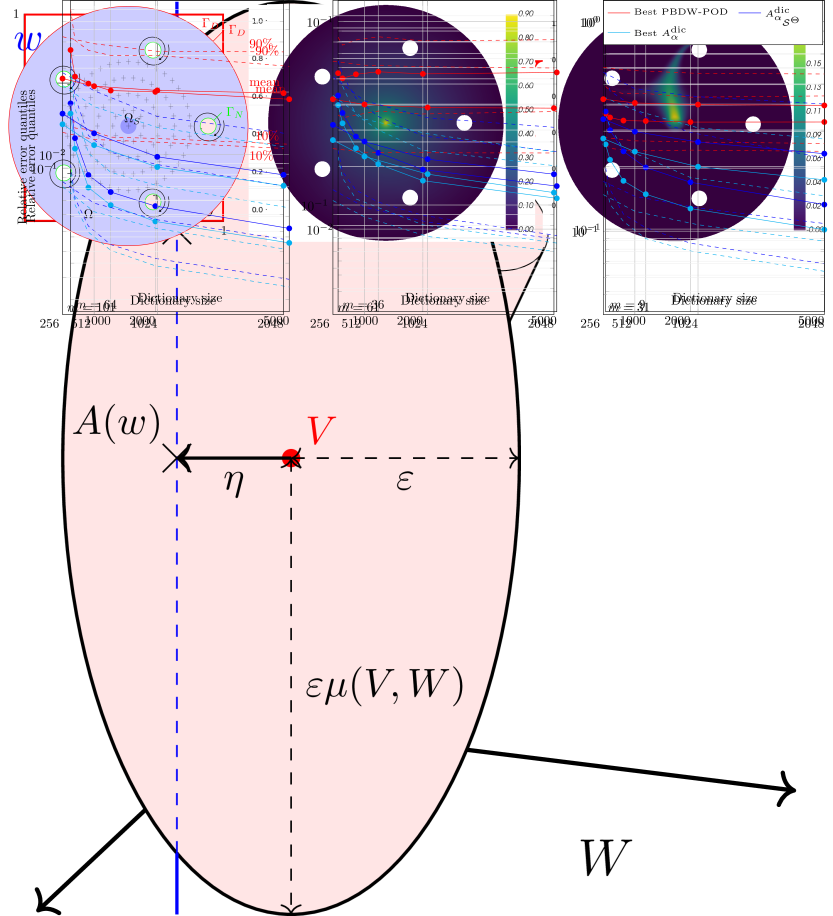
Figure 3: Evolution of the recovery errors in $U$-norm, on $500$ test snapshots, with growing dictionary sizes. We compare the PBDW recovery based on the best adaptive POD truncation (red), the dictionary-based recovery with randomized selection criterion (blue), as well as the best one produced by the LARS algorithm (cyan). The dotted lines are the $10\%$ and $90\%$ error quantiles, and the full line is the mean error.

6.2 Advection-diffusion

In this subsection we consider an advection diffusion problem with multiple transport phenomena, inspired from [4]. It models a heat diffusion and advection in a 2D domain $\Omega=\mathcal{B}(0,1.5)\setminus\bigcup_{i=1}^{5}\Omega_{i}$, with $\Omega_{i}=\mathcal{B}(x^{(i)},0.1)$ a ball of radius $0.1$ centered at $x^{(i)}=(\cos(2i\pi/5),\sin(2i\pi/5))$, for $1\leq i\leq 5$. A constant source term is considered on the circular subdomain $\Omega_{S}=\mathcal{B}(0,0.1)$. The (parametric) advection field $\mathcal{V}$ is a sum of $5$ potential fields around the domains $\Omega_{i}$. The unknown temperature field $u$ satisfies the equations

$$\left\{\begin{aligned} -\kappa\Delta u+\mathcal{V}(\xi)\cdot\nabla u=~{}&\frac{100}{\pi}\mathbbm{1}_{\Omega_{S}}&\text{in }&\Omega,\\ u=~{}&0&\text{on }&\Gamma_{D},\\ n\cdot\nabla u=~{}&0&\text{on }&\Gamma_{N},\end{aligned}\right.$$ (55)

with a diffusion coefficient $\kappa=0.01$ and the advection field

$$\mathcal{V}(\xi)=\sum_{i=1}^{5}\frac{1}{\|x-x^{(i)}\|}\Big{(}\xi_{i}e_{r}(x^{(i)})+\xi_{i+5}e_{\theta}(x^{(i)})\Big{)},$$

where $e_{r}(x^{(i)})$ and $e_{\theta}(x^{(i)})$ are the basis vectors of the polar coordinate system centered at $x^{(i)}$. Dirichlet boundary conditions are imposed on $\Gamma_{D}=\partial\mathcal{B}(0,1.5)$ and homogeneous Neumann conditions are imposed on $\Gamma_{N}=\Omega\setminus\Gamma_{D}$. The parameter $\xi$ is chosen uniformly in $\mathcal{P}=[-1,-\frac{1}{2}]^{5}\times[-2,-1]^{5}$. The problem is discretized using Lagrange $\mathbb{P}_{1}$ finite elements on a triangular mesh refined around the pores, leading to $\mathcal{N}=152~{}297$ degrees of freedom. The operator and right-hand admit the affine representations

$$\mathbf{B}(\xi)=\mathbf{B}^{(0)}+\sum_{i=1}^{10}\xi_{i}\mathbf{B}^{(i)},\hskip 14.22636pt\mathbf{f}(\xi)=\mathbf{f}.$$ (56)

We consider $101$ sensors. A first sensor is placed at point $(0,0)$, and for $1\leq j\leq 4$, $10\times j$ sensors are placed uniformly on a circle of radius $0.2\times j$ centered at $(0,0)$. The sensor width is chosen as $\sigma=2.10^{-2}$. The problem can be visualized in Figure 4.

Figure 4: The advection diffusion problem. On the left, the geometry of the problem, with sensors locations (crosses) and advection fields (circular arrows). On the middle, the (normalized) Riesz representer of the central sensor. On the right, an example of snapshot.

We consider 3 different values for $m$: $101$, $61$ and $31$. For $m=101$ every sensors are used, for $m=61$ we dropped the sensors of the outer circle, and for $m=31$ we dropped the sensors of the two outer circles. We computed a set $\mathcal{M}_{\text{prior}}$ of $2048$ snapshots to form our prior knowledge on the manifold $\mathcal{M}$. We test the performances of our dictionary-based approach with dictionaries of size $K\in\{256,512,1024,2048\}$. We choose $\mathbf{\Omega}=\mathbf{\Omega}_{2}\mathbf{\Omega}_{1}$ with $\mathbf{\Omega}_{1}$ a P-SRHT embedding with $k^{\prime}=16~{}263$ rows and $\mathbf{\Omega}_{2}$ a Gaussian embedding with $k=850$ rows. The numerical results are summarized in Fig. 5.

Figure 5: Evolution of the recovery errors in $U$-norm, on $500$ test snapshots, with growing dictionary sizes. We compare the PBDW recovery based on the best adaptive POD truncation (red), the dictionary-based recovery with randomized selection criterion (blue), as well as the best one produced by the LARS algorithm (cyan). The dotted lines are the $10\%$ and $90\%$ error quantiles, and the full line is the mean error.

6.3 Observations

From the numerical results of the previous subsections, we draw three main observations. Firstly, our dictionary-based approach with randomized selection criterion outperformed the best possible POD-based PBDW recovery, even with reasonable sizes of dictionary. Secondly, increasing the latter improves global performances. Secondly, increasing the number of measurements $m$ improves the relative performance gain of both the best recovery map $A^{\text{dic}}_{\alpha}$ and the recovery map $A^{\text{dic}}_{\alpha_{\mathcal{S}^{\Theta}}}$, compared to the best POD-based multispace recovery. Thirdly, the relative difference of performances between the two dictionary-based recoveries decreases when $m$ grows. This may be explained by an increase of $\mu(\mathcal{M},W)$ in Corollary 5.

Finally, it is important to note that, in Section 6.2, with the rather large $\mathcal{N}$ and $K$ involved, the randomized approach from Section 4 was crucial to efficiently evaluate online $\mathcal{S}^{\Theta}$ while requiring a moderate offline cost, which is not possible with $\mathcal{S}$. On the other hand, in Section 6.1, $\mathcal{N}$ was rather small and we could compute $\mathcal{S}$ online by solving the least-squares system of size $\mathcal{N}\times d$ with rather low computational cost.

7 Conclusions

In this work, we proposed a dictionary-based model reduction approach for inverse problems, similar to what already exists for direct problems, with a near-optimal subspace selection based on some surrogate distance to the solution manifold, among the solutions of a path of $\ell_{1}$-regularized problems. We focused on the framework of parameter-dependent operator equations with affine parameterization, for which we provided an efficient procedure based on randomized linear algebra, ensuring stable computation while preserving theoretical guarentees.

Future work shall study the performances of our approach in a noisy observations framework. One may also consider a bi-dictionary approach, in which both the observation space and the background space would be selected adaptively with a dictionary-based approach.

References

• [1] Alexandr Andoni, Piotr Indyk, Thijs Laarhoven, Ilya Razenshteyn, and Ludwig Schmidt. Practical and Optimal LSH for Angular Distance. In Advances in Neural Information Processing Systems, volumeย 28. Curran Associates, Inc., September 2015.
• [2] Oleg Balabanov and Anthony Nouy. Randomized linear algebra for model reduction. Part I: Galerkin methods and error estimation. Adv Comput Math, 45(5-6):2969โ€“3019, December 2019.
• [3] Oleg Balabanov and Anthony Nouy. Preconditioners for model order reduction by interpolation and random sketching of operators. arXiv:2104.12177 [cs, math], April 2021.
• [4] Oleg Balabanov and Anthony Nouy. Randomized linear algebra for model reductionโ€”part II: Minimal residual methods and dictionary-based approximation. Adv Comput Math, 47(2):26, April 2021.
• [5] Peter Binev, Albert Cohen, Wolfgang Dahmen, Ronald DeVore, Guergana Petrova, and Przemyslaw Wojtaszczyk. Data Assimilation in Reduced Modeling. SIAM/ASA J. Uncertainty Quantification, 5(1):1โ€“29, January 2017.
• [6] Peter Binev, Albert Cohen, Olga Mula, and James Nichols. Greedy Algorithms for Optimal Measurements Selection in State Estimation Using Reduced Models. SIAM/ASA J. Uncertainty Quantification, 6(3):1101โ€“1126, January 2018.
• [7] Andreas Buhr, Christian Engwer, Mario Ohlberger, and Stephan Rave. A numerically stable a posteriori error estimator for reduced basis approximations of elliptic equations. preprint, 2014.
• [8] Fabien Casenave, Alexandre Ern, and Tony Leliรจvre. Accurate and online-efficient evaluation of the a posteriori error bound in the reduced basis method. ESAIM: M2AN, 48(1):207โ€“229, January 2014.
• [9] Yanqing Chen, Timothyย A Davis, Williamย W Hager, and Sivasankaran Rajamanickam. Algorithm 887: CHOLMOD, Supernodal Sparse Cholesky Factorization and Update/Downdate. ACM Transactions on Mathematical Software, 35(3):14, October 2018.
• [10] Albert Cohen, Wolfgang Dahmen, Ronald DeVore, Jalal Fadili, Olga Mula, and James Nichols. Optimal Reduced Model Algorithms for Data-Based State Estimation. SIAM J. Numer. Anal., 58(6):3355โ€“3381, January 2020.
• [11] Albert Cohen, Wolfgang Dahmen, Olga Mula, and James Nichols. Nonlinear Reduced Models for State and Parameter Estimation. SIAM/ASA J. Uncertainty Quantification, 10(1):227โ€“267, March 2022.
• [12] Albert Cohen, Matthieu Dolbeault, Olga Mula, and Agustin Somacal. Nonlinear approximation spaces for inverse problems, October 2022.
• [13] Bradley Efron, Trevor Hastie, Iain Johnstone, and Robert Tibshirani. Least angle regression. Ann. Statist., 32(2), April 2004.
• [14] Jensย L. Eftang, Davidย J. Knezevic, and Anthonyย T. Patera. An hp certified reduced basis method for parametrized parabolic partial differential equations. Mathematical and Computer Modelling of Dynamical Systems, 17(4):395โ€“422, August 2011.
• [15] Jensย L. Eftang, Anthonyย T. Patera, and Einarย M. Rรธnquist. An โ€$hp$โ€ Certified Reduced Basis Method for Parametrized Elliptic Partial Differential Equations. SIAM J. Sci. Comput., 32(6):3170โ€“3200, January 2010.
• [16] Loic Giraldi and Anthony Nouy. Weakly Intrusive Low-Rank Approximation Method for Nonlinear Parameter-Dependent Equations. SIAM J. Sci. Comput., 41(3):A1777โ€“A1792, January 2019.
• [17] C.ย Herzet and M.ย Diallo. Performance guarantees for a variational โ€œmulti-spaceโ€ decoder. Adv Comput Math, 46(1):10, February 2020.
• [18] Sven Kaulmann and Bernard Haasdonk. Online greedy reduced basis construction using dictionaries. In VI International Conference on Adaptive Modeling and Simulation ADMOS 2013, pageย 12, March 2013.
• [19] Anders Logg and Garthย N. Wells. DOLFIN: Automated finite element computing. ACM Trans. Math. Softw., 37(2):1โ€“28, April 2010.
• [20] Yvon Maday, Ngoc Cuongย Nguyen, Anthony T.ย Patera, and S.ย H.ย Pau. A general multipurpose interpolation procedure: The magic points. Communications on Pure & Applied Analysis, 8(1):383โ€“404, 2009.
• [21] Yvon Maday, Anthonyย T. Patera, Jamesย D. Penn, and Masayuki Yano. A parameterized-background data-weak approach to variational data assimilation: Formulation, analysis, and application to acoustics. Int. J. Numer. Meth. Engng, 102(5):933โ€“965, May 2015.
• [22] Yvon Maday, Anthony T, Jamesย D Penn, and Masayuki Yano. PBDW State Estimation: Noisy Observations; Configuration-Adaptive Background Spaces; Physical Interpretations. ESAIM: Proc., 50:144โ€“168, March 2015.
• [23] Julien Mairal, Francis Bach, Jean Ponce, and Guillermo Sapiro. Online dictionary learning for sparse coding. In Proceedings of the 26th Annual International Conference on Machine Learning, pages 689โ€“696, Montreal Quebec Canada, June 2009. ACM.
• [24] Renรฉ Milk, Stephan Rave, and Felix Schindler. pyMOR โ€“ Generic Algorithms and Interfaces for Model Order Reduction. SIAM J. Sci. Comput., 38(5):S194โ€“S216, January 2016.
• [25] Holger Rauhut and Rachel Ward. Interpolation via weighted $l_1$ minimization, March 2015.
• [26] Tommaso Taddei. An Adaptive Parametrized-Background Data-Weak approach to variational data assimilation. ESAIM: M2AN, 51(5):1827โ€“1858, September 2017.
• [27] V.ย N. Temlyakov. Nonlinear Kolmogorov widths. Math Notes, 63(6):785โ€“795, June 1998.
• [28] Ryanย J. Tibshirani. The lasso problem and uniqueness. Electron. J. Statist., 7(none), January 2013.
• [29] Joelย A. Tropp. Improved analysis of the subsampled randomized Hadamard transform. Adv. Adapt. Data Anal., 03(01n02):115โ€“126, April 2011.
• [30] Davidย P. Woodruff. Computational Advertising: Techniques for Targeting Relevant Ads. FNT in Theoretical Computer Science, 10(1-2):1โ€“157, 2014.
• [31] Olivier Zahm and Anthony Nouy. Interpolation of Inverse Operators for Preconditioning Parameter-Dependent Equations. SIAM J. Sci. Comput., 38(2):A1044โ€“A1074, January 2016.
• [32] Hui Zhang, Wotao Yin, and Lizhi Cheng. Necessary and Sufficient Conditions of Solution Uniqueness in 1-Norm Minimization. J Optim Theory Appl, 164(1):109โ€“122, January 2015.