AutoEn: An AutoML method based on ensembles of predefined Machine Learning pipelines for supervised Traffic Forecasting

Abstract

Intelligent Transportation Systems are producing tons of hardly manageable traffic data, which motivates the use of Machine Learning (ML) for data-driven applications, such as Traffic Forecasting (TF). TF is gaining relevance due to its ability to mitigate traffic congestion by forecasting future traffic states. However, TF poses one big challenge to the ML paradigm, known as the Model Selection Problem (MSP): deciding the most suitable combination of data preprocessing techniques and ML method for traffic data collected under different transportation circumstances. In this context, Automated Machine Learning (AutoML), the automation of the ML workflow from data preprocessing to model validation, arises as a promising strategy to deal with the MSP in problem domains wherein expert ML knowledge is not always an available or affordable asset, such as TF. Various AutoML frameworks have been used to approach the MSP in TF. Most are based on online optimisation processes to search for the best-performing pipeline on a given dataset. This online optimisation could be complemented with meta-learning to warm-start the search phase and/or the construction of ensembles using pipelines derived from the optimisation process. However, given the complexity of the search space and the high computational cost of tuning-evaluating pipelines generated, online optimisation is only beneficial when there is a long time to obtain the final model. Thus, we introduce AutoEn, which is a simple and efficient method for automatically generating multi-classifier ensembles from a predefined set of ML pipelines. We compare AutoEn against Auto-WEKA and Auto-sklearn, two AutoML methods commonly used in TF. Experimental results demonstrate that AutoEn can lead to better or more competitive results in the general-purpose domain and in TF.

1 Introduction

Sensing and telecommunications technologies generate vast volumes of data that motivate the use of data-driven approaches, particularly in Machine Learning (ML), to analyse this data. Like other research areas, Intelligent Transportation Systems (ITSs) announce the production of tons of hardly manageable traffic data that can be used by different applications such as traveller information systems or Traffic Forecasting (TF) schemes. Recently, TF has been gaining relevance due to its ability to deal with traffic congestion by forecasting future states of traffic measures (e.g., travel time) [1]. From a ML perspective, TF is approached through learning and approximating a mapping function from historical data to make traffic predictions when facing unseen data.

TF poses two main challenges to the ML paradigm. First, traffic data can be collected in multiple formats (e.g., traffic-counting measures, GPS tracks) and under different transportation circumstances (e.g., urban, freeway). These characteristics influence the performance of ML methods, and choosing the most competitive method from a set of candidates brings human effort and time costs. Second, raw traffic data usually needs to be preprocessed before being analysed. Therefore, deciding the most suitable combination of data preprocessing techniques and ML method (also known as the Model Selection Problem, MSP) is a time-consuming task that demands specialised ML knowledge, which is an asset not always available. In this context, Automated Machine Learning (AutoML) is a promising path to address the MSP in TF. AutoML is an emerging area in ML that seeks to automate the ML workflow from data preprocessing to model validation [2]. Such automation provides robust AutoML methods that enable people, with either little or no specialised ML knowledge, to integrate ML solutions into data-driven processes. The latter is known as the democratisation of ML [2], and it is aligned with the actual purpose of Artificial Intelligence: to learn and act automatically without human intervention [3].

Recent literature reports a wide variety of AutoML methods, where only a few automatise the construction of complete ML pipelines [4, 5, 6]. In the transportation area, to the best authors’ knowledge, only a few papers have used general-purpose AutoML methods (agnostic methods w.r.t. to the problem domain where the input data comes from) for TF [7, 8, 9, 10]. Those studies have used AutoML techniques that usually generate ML pipelines using an online search strategy, that is, a search strategy that takes place after the input dataset has been provided. In some cases [7, 8, 10], this online search can be purely based on optimisation approaches that test different promising combinations of pipelines structures from a predefined base of preprocessing and ML algorithms. Here the aim is to minimise or maximise a predefined performance measure (e.g., Auto-WEKA [11]). Alternatively, the study of [9] used Auto-sklearn, whose online search is complemented with meta-learning and ensemble learning [12]. This AutoML method first extracts meta-features of the input dataset at hand, providing information such as the number of instances, classes or entropy, among others. From these meta-features, meta-learning identifies suitable candidates for pipeline structures from a predefined knowledge base that stores meta-features for different datasets and pipelines that are likely to perform well on them. Then, the candidate pipelines are used for a warm-start of the optimisation approach. Lastly, the best-performing pipelines found during the optimisation search are used to build an ensemble of models.

As it can be observed from those studies in TF, the online search of AutoML generally uses optimisation as the core engine for generating and tuning pipelines. However, optimising ML pipelines is a difficult task for two reasons: (1) the complexity of the search space and (2) the evaluation cost. Regarding the search space, its complexity is given by the heterogeneity of the domains of decision variables (e.g. categorical, binary, integer). As for the evaluation cost, it is due to the need to train and validate the model on the dataset to obtain its performance. For these reasons, optimising ML pipelines usually requires a long time to provide good results, especially for big datasets. However, a lengthy optimisation process may be prone to overfitting [8, 13, 10]. Although meta-learning has arisen as a promising strategy to solve some previous problems, especially the computational cost of pipeline optimisation, this approach also presents a drawback. Finding a representative set of meta-features to characterise very diverse datasets is challenging. The latter can lead to the risk that in very different ML tasks to those stored in the knowledge base, such as TF, the meta-learning component and its meta-features may suggest pipelines that do not work correctly on the dataset at hand [9].

Considering the limitations mentioned above, the automated process of generating and testing ML pipelines in TF shows a wide margin of improvement. The latter offers the opportunity to develop new and novel AutoML approaches toward more robust and efficient strategies for the automated construction of ML pipelines, which can be better adapted to specific problem domains, such as TF. Therefore, this paper introduces a simple strategy for AutoML that does not require a pipeline optimisation process (making it more scalable and less prone to overfitting) and does not rely on extracted meta-features. The proposed approach, named AutoEn, is a simple yet effective ensemble-based AutoML method for the automatic generation of ensembles [14], from a predefined set of pipelines composed of a sequence of preprocessing techniques plus one ML classifier. The main contributions of this paper are listed below.

• To demonstrate the suitability and competitiveness of AutoEn and its simple online search strategy based on the construction of ensembles of multiple classifiers rather than in the search, construction and tuning of individual pipelines usually done by current AutoML methods in TF.

• To demonstrate the contributions that AutoEn brings to TF. To this end, we test AutoEn against Auto-sklearn in various multi-class TF problems previously used in the transportation literature.

• To test the performance and determine the competitiveness of AutoEn in the general-purpose domain (using data not related to the TF domain). This comparison is made using the first version of the so-called AutoML benchmark [13], which is composed of diverse binary and multi-class supervised classification problems.

The rest of this paper is structured as follows. Section 2 presents background and related work about AutoML, emphasising methods that automatise complete ML pipelines for TF. Section 2 introduces the AutoML method proposed in this paper. Later on, Section 4 exposes the experimental framework and Section 5 analyses the results obtained. Finally, conclusions are discussed in Section 6.

2 Background and Related Work

2.1 Approaches for the automatic construction of complete ML workflows

ML is the field focused on algorithms able to carry out prediction/classification tasks employing an automatic learning process without the need of being explicitly programmed by human intervention [15, 3]. Applications like e-mail spam and malware filtering, automatic speech recognition, and predictive maintenance in industry, among others, are built upon ML. As a common denominator, all these applications required well-designed and efficient ML pipelines that include data preprocessing as a critical factor [16, 17].

Following the definition of [6], a ML pipeline can be defined as a combination of data preprocessing methods and classifiers, with configuration of hyperparameters, that maps input data $X$ into target values $Y$ (this is known as the MSP). In this context, time, human effort, and computational capabilities are required to generate, train, and test a ML workflow because no ML pipeline can be competitive on every supervised learning task it faces. The MSP is usually approached by ML experts or by practitioners who follow a trial and error strategy, causing the success of ML to happen at a elevated costs due to the resources consumed in this task [5]

Thus, AutoML is by far a suitable strategy to deal with the MSP, while allowing to decrease human effort and bias, and computational costs by bulding ML workflows more efficiently. AutoML is an area of ML that aims at automatically finding the best combination of preprocessing techniques, ML algorithm and its hyperparameters, without being specialised in the problem domain wherein this data comes from (this is known as general-purpose AutoML) [2].

AutoML literature [5, 2, 6] presents a variety of AutoML methods. They differ depending on which stages of a ML pipeline is automated, for example, data preprocessing [18, 19, 20], algorithm selection and hyper-parameters [21, 22, 11, 23], or the entire pipeline. This paper focuses on automating ML pipelines composed of data preprocessing techniques and a classifier algorithm with their respective hyperparameter configuration.

In the literature of the automatic construction of ML pipelines, we can usually find three main categories of AutoML methods to automatise the construction of ML pipelines. The first is purely based on optimisation approaches that test different promising combinations of algorithms from a predefined base of ML classifiers to minimise or maximise a performance measure [24, 11]. Alternatively, there are AutoML methods whose online search is complemented with learning strategies like meta-learning [25]. These techniques first extract meta-features of the input dataset (e.g., number of instances, features, classes). Then, from these meta-features, meta-learning identifies suitable candidates for pipeline structures from a predefined knowledge base that stores meta-features for different datasets and ML models that are likely to perform well on them. Then, the candidate models are typically used to warm-start an optimisation process. In addition, other AutoML methods use ensemble learning to build diverse sets of classifiers from predefined portfolios of ML algorithms [12]. These ensemble approaches have proven to be more robust than other AutoML methods, such as the case of Auto-Gluon, which incorporates an ensemble learning strategy based on multi-layer stacking [26].

2.2 AutoML in Traffic Forecasting

In the transportation area, to the best authors’ knowledge, only a few studies have used AutoML concepts in TF [7, 8, 10, 9]. The first attempt was introduced by Vlahogianni et al.[7]. They proposed a meta-modelling technique that automatically recommends a classifier for traffic prediction. This method was based on surrogate modelling and a genetic algorithm with an island model. The authors automatised the algorithm selection and the hyper-parameter setting, without including the preprocessing stage, as this paper does. The study of Vlahogianni et al.[7] can be considered the first incursion of AutoML principles in the TF domain.

After that, Angarita et al. in [8, 10, 9] brought AutoML state-fo-the-art concepts to the TF area. In these three studies, the authors determined the extent to which general-purpose AutoML can be competitive against ad hoc methods in domain-related problems. Specifically, they researched whether it is valuable to use general-purpose AutoML already available in the literature (they used Auto-WEKA and Auto-sklearn) or develop domain-related AutoML for ITSs, using TF as a case study.

In the case of [10] and [8], the authors used Auto-WEKA, an AutoML method that applies sequential model-based Bayesian optimisation to find optimal ML pipelines for TF. Both papers tested the performance of Auto-WEKA against the classic model selection approach, which consists of selecting the best of a set of algorithms to predict traffic by trial and error. Lastly, Angarita et al. [9] used Auto-sklearn version one, a state-of-the-art AutoML method whose search strategy of pipelines uses Bayesian optimisation, meta-learning and ensemble learning. The authors tested this method in multi-class imbalanced classification problems for different time horizons and for freeway and urban environments.

As a common factor, the core of pipeline search strategies used by the AutoML methods tested in [7, 8, 10, 9] is focused on generating and fine-tuning individual pipelines. Nonetheless, this online optimisation of pipelines is a demanding process because 1) it involves complex search spaces; 2) the evaluation of the objective function usually is computationally expensive; and 3) to establish a priori the best time budget for the optimisation process is a difficult task since in complex or big datasets collecting good pipelines can require a long time, while in small or simpler datasets an excessive time budget is prone to overfitting [8, 10]. Although Auto-sklearn combines meta-learning with optimisation to reduce the impact of some of these issues, it has a drawback. Defining a set of meta-features that characterises very diverse datasets is difficult without solid evidence to guide this design process. In this way, there is a risk that in very different supervised learning tasks to those included in the meta-knowledge base, such as the case of TF, the meta-learning component may suggest pipelines that are not competitive to warm-start the optimisation process [9].

Those in-depth analyses of general-purpose AutoML in TF allowed identifying a set of strengths and weaknesses of AutoML when dealing with supervised traffic prediction. Therefore, in this paper, we introduce AutoEn, a new and novel AutoML method that overcomes the drawbacks (related to optimisation and meta-learning) identified by[8, 10, 9]. AutoEn enhances the AutoML state-of-the-art in TF by automatically generating ensembles during the online search phase of AutoML. Thus, rather than focusing on single pipelines, we approach the finding of solid ensembles of multiple pipelines, which is a more straightforward and efficient strategy to deal with the issues mentioned above. The latter enables us to improve the performance of AutoML in TF, which can also benefit the performance of AutoML in the general-purpose domain.

3 AutoEn: An AutoML method based on Ensemble learning

3.1 Motivation

As we stated before, the core of the existing AutoML methods used in TF is the optimisation of individual ML pipelines, which could be enhanced with a preliminary stage based on meta-learning. However, the current solutions suffer from several issues that motivate the design of AutoEn.

• Optimisation - Overfitting issues: Optimising pipelines is supposed to require long time budgets to find competitive solutions. However, previous research has corroborated that longer execution times may cause overfitting issues due to hyperparameters tuning [8, 13, 10]. Therefore, higher execution times do not always lead to better results as we could expect. In addition, for medium- and small-size datasets, competitive pipelines can be quickly found without the need to allocate long time budgets for the optimisation search. Thus, optimising pipelines can be expensive when the goal is to make good enough predictions.

• Optimisation - Reduced scalability: Although long time budgets of optimisation may be prone to return pipelines with overfitting issues, other times the results can be promising. Particularly, when optimisation deals with small- or medium-size datasets, many diverse pipeline structures can be generated, tuned and tested because the complexity of the learning task at hand is influenced by its data size. On the other hand, the latter may stop happening as the data size grows. In this scenario, it is harder to tune and test multiple pipelines, as the optimisation becomes expensive, and the set of candidate pipelines could decrease, which ends up affecting the performance of the final solutions.

• Meta-learning - Representativeness of Meta-features: Meta-learning can potentially reduce the cost of the optimisation process. Nevertheless, there is a risk that the meta-features can only describe the learning tasks in the meta-knowledge base. The latter is understandable because it is difficult to find a set of meta-features good enough to characterise very diverse datasets. Therefore, there is a risk that for supervised learning tasks not similar to the ones stored in the meta-knowledge base, the meta-learning component recommends pipelines that do not perform as well as expected in specific supervised learning tasks [9]. Thus, the optimisation process could be warm-started with pipelines that are not competitive on the input data.

Keeping in mind the motivations presented above, we want to conceive a competitive and straightforward AutoML method that adjusts to the complexity of the data without the need to define a time budget for its execution. This means that for small- and medium-size datasets, the method can find quick solutions; conversely, for large datasets, the method may take longer time to find competitive pipelines. The aforementioned condition could be satisfied by not only suggesting single pipelines whose performance could vary drastically from one learning task to another. In this sense, we propose an AutoML method based on the search and construction of ensembles of multi-classifiers that do not commit to a single ML workflow. Accomplishing such a goal requires the ensemble contains models that individually are different in nature and strong in making individual predictions. Therefore, we introduce AutoEn, an AutoML method based on ensemble learning for combining high-performance instantiations of different pipelines.

3.2 AutoEn design and workflow

Figure 1 introduces the architecture of AutoEn. This AutoML replaces the online search and optimisation of individual pipelines with the automated generation of ensembles. Similarly to Auto-sklearn, it has in its inner structure a base of diverse pipelines that were trained on different learning tasks during the construction of AutoEn (the off-line phase of AutoML). The pipelines within this base consist of a sequence of data preprocessing techniques and a classifier algorithm. The underlying idea of using a set of predefined pipelines is offering ML workflows different in nature for every learning task, which are less prone to overfitting issues. Unlike Auto-sklearn, we will not use meta-features to decide what pipelines are part or not of the ensemble construction.

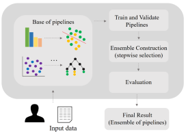
Figure 1: General workflow of AutoEn that is composed of two main blocks: 1) a set of predefined pipelines trained on different learning tasks and 2) an ensemble component that generates a multi-classifier system, from the set of pipelines, when a new dataset comes in.

A meta-learning approach should be able to assist us in finding the most promising pipelines to be part of the ensemble. However, we observed in [9] that this idea can only correctly work under a good enough set of meta-features able to characterise very different datasets, which unfortunately is not always the case. To avoid relying on meta-features, when new input data comes in AutoEn, it assesses the performance of the base of pipelines on a validation set. The pipelines can or cannot be part of the ensemble construction depending on their validation errors. Thus, we avoid the drawbacks of meta-learning when facing very diverse learning tasks.

Details about the automatic selection and construction of the ensemble based on these pipelines is presented in Figure 2. In step (1), it receives a new and unseen dataset that later in step (2) is split into train, validation and test sets. Then, in step (3), we retrieve the set of available ML pipelines.

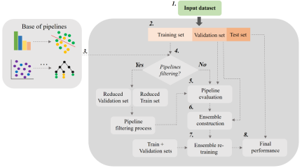
Figure 2: Automated selection and construction of the ensemble based on the set of pipelines .

Having the list of optimised pipelines at hand, in step (4), it is possible to filter them to improve the computational efficiency or not. The latter decision implies either directly training the complete list of pipelines on the training set (”No” path) or reducing the list to have a smaller set (”Yes” path) to enhance the computational efficiency. The former option is the default mode of our AutoML method, whilst the latter implies selecting a sample of the training set (dashed line in Figure 2), which is divided into training and validation set (reduced train and validation set in Figure 2). The aim is to filter the pipelines and choose the fastest ones.

After selecting the complete list of pipelines or a reduced version, the next step is training the available pipelines in the complete train set and ranking them according to their errors in the validation set (step 5). After that, we build an ensemble from this set of trained pipelines (step 6). Finally, we implemented the ensemble selection approach introduced by [27]. The latter is a greedy procedure that starts from an empty ensemble and then iteratively adds the model that maximises ensemble performance in the same validation set in which the pipelines were previously assessed.

For our AutoEn, we initialise the ensemble with one element, the pipeline with the highest validation set performance. Then, from the one-element ensemble, we start to append new pipelines, with uniform weights, to the one-element ensemble until reaching a predefined ensemble size. It is essential to note that the inclusion of new pipelines in the ensemble allows repetitions; this means one high-performance pipeline can appear multiple times in the final ensemble. Finally, in step (7), the pipelines that composed the ensemble are re-trained on training+validation partitions to make classification on the unseen test set finally. For this final step, the pipelines that appear multiple times in the ensemble are only re-trained once; thus, we can decrease the computational cost of this final step.

4 Experimental Framework

This paper seeks to answer the question of whether it is possible to conceive an AutoML framework based on multi-classifier ensembles and able to make good enough predictions in supervised classification problems, specifically for the case of supervised TF. We test AutoEn in the general-purpose domain and the TF problems to accomplish such a purpose.

Regarding the general-purpose area, we compare AutoEn against Auto-sklearn and Auto-WEKA, two well-established AutoML methods based on pure optimisation and meta-learning with optimisation, which have been used in TF literature previously. We evaluate the performance of AutoEn versus the results of Auto-sklearn and Auto-WEKA reported in the AutoML benchmark published by [13]. This benchmark is an open-source AutoML framework that uses public datasets to compare AutoML methods thoroughly.

Regarding the TF domain, we demonstrate that AutoEn enhances the performance of AutoML in TF. To this end, we test AutoEn against Auto-sklearn in various multi-class TF problems that were previously used in [9]. The reason to only consider Auto-sklearn is that this AutoML method overcomes the limitations of AutoML techniques based only on optimisation, such as in the case of Auto-WEKA.

The rest of this section presents the elements related to the two experiments designed to test and assess the competitiveness of AutoEn. First, we provide details of the datasets chosen for the experimentation. Then, we introduce the measures employed to evaluate the performance of the methods. Finally, we present the methods used for comparison.

4.1 Supervised learning problems

4.1.1 General-purpose datasets

We use 16 datasets of binary classification problems and 12 multi-class problems from the AutoML benchmark developed by [13]. The total of 28 datasets are not related to TF and were used in previous AutoML papers [11], AutoML competitions [28] and ML benchmarks [29]. The datasets vary in the number of samples and features by orders of magnitude and the occurrence of numeric features, categorical features and missing values. The current list of datasets is available on OpenML [30]

Tables 1 and 2 present a summary of binary and multi-class datasets used for this experimentation. They show the number of features and instances (Feat. - Instan.), the number of numeric and nominal features (Num. Feat. and Nom. Feat), and the number of missing values (Missing Val.) on each dataset.

Table 1: Binary datasets

dataset	Feat. - Instan.	Num. Feat.	Num. Feat.	Missing Val.
adult	15 - 48842	6	9	6465
amazon_employ	10 - 32769	0	10	0
albert	79 - 425240	26	53	2734000
apsfailure	171 - 76000	170	1	1078695
bank-mark	17 - 45211	7	10	0
blood-transf	5 - 748	4	1	0
christine	1637 - 5418	1599	38	0
credit-g	21 - 1000	7	14	0
higgs	29 - 98050	28	1	9
jasmine	145 - 2984	8	137	0
kc1	22 - 2109	21	1	0
kr-vs-kp	37 - 3196	0	37	0
nomao	119 - 34465	89	30	0
numerai28.6	22 - 92320	21	1	0
phoneme	6 - 5404	5	1	0
sylvine	21 - 5124	20	1	0

Table 2: Multi-class datasets

dataset	Feat. - Instan	Num. Feat.	Nom. Feat.	Classes
car	7 - 1728	0	7	4
cnae-9	857 - 1080	856	0	9
connect-4	43 - 67557	0	43	3
dilbert	2001 - 10000	2000	1	5
fashion-mnist	785 - 70000	784	1	10
jannis	55 - 83733	54	1	4
jungle	7 - 44819	6	1	3
mfeat-factors	217 - 2000	216	1	10
segment	20 - 2310	19	1	7
shuttle	10 - 58000	9	1	7
vehicle	19 - 846	18	1	4
volkert	181 - 58310	180	1	10

4.1.2 Traffic Forecasting datasets

We considered freeway and urban scenarios for these datasets. In the freeway case, the data was taken from Caltrans Performance Measurement System ; meanwhile, for the urban enviroment the data was retrieved from Madrid Open Data Portal . In freeway and urban cases, the traffic measure was three months of speed in aggregation times of 5 and 15 minutes, respectively.

All datasets were enriched with Calendar Data (Day of the week and Minute of the day). In addition to Calendar dDta (CD), freeway and urban datasets can be composed of only temporal traffic data (Temporal traffic data, T) from the target location or traffic data from the target location and four downstream locations (Temporal and Spatial traffic data, TS). More details of these datasets can be consulted in [9, 10].

The target output of all datasets is modelled as multi-class classification problem where the aim is to predict the Level of Service (LoS). LoS is a traffic measure topically used to describe the quality of traffic flows. That categorization of traffic is done using categorical levels, which range from A to E in a gradual way [31]. In the freeway case, the time horizons of predictions are 5, 15, 30, 45, and 60 minutes using a data granularity of 5 minutes. For the urban datasets, the forecasting time steps are 15, 30, 45, and 60 minutes with a data granularity of 15 minutes.

Table 3 presents a summary of the datasets described above. The description includes the number of instances, features, and the number of classes of each dataset.

Table 3: Traffic Forecasting datasets

Environment	datasets	Num. Instan.	Featurs	Classes
Freeway	T+CD in time horizons of 5, 15, 30, 45, 60 minutes	[10927 - 9906]	13	4
	TS+CD in time horizons of 5, 15, 30, 45, 60 minutes	[10927 - 9906]	28	3
Urban	T+CD in time horizons of 15, 30, 45, 60 minutes	[2684-2634]	13	3
	TS+CD in time horizons of 15, 30, 45, 60 minutes	[2684-2634]	28	3

4.2 Performance metrics and Hardware choice

4.2.1 General-purpose domain

• Metrics: For the results of this paper, we follow the same experimental set-up proposed in the AutoML benchmark to make fair comparisons, and therefore, we use the same performance measures. The area under the receiver operator curve (roc_auc_score) is used for binary classification problems and log loss_score for multi-class problems. Besides, both measures are averages of ten-fold cross-validation.

• Hardware choice and resource specifications: We opted to use a cluster based on Centos 7.6 with kernel 3.10.0, and usig QuadCore Intel Xeon processors, with 16 cores and 16 GB of RAM each. Here, we highlight that despite the multi-core character of the CPU, the implementation of AutoEn is single-core.

• Computational time: To measure how much time AutEn takes since new input data comes in until it makes final predictions, we measure the execution time in seconds extracted from the system clock. Concretely, we start to measure this time when AutoEn receives the input data from making the data partitions until it outputs the final classification of the ensemble built during the online search of the method.

• Statistical tests: We used non-parametric statistical tests to assess the differences in performance of the methods. Two statistical tests are considred following the guidelines proposed in [32]. First, Friedman’s test for multiple comparisons is applied to check whether there are differences among the methods. Then, Holm’s test is used to check whether the differences in the Friedman ranking are statistically significant or not.

4.2.2 Traffic Forecasting

• Metrics: We use for this case study the same experimental framework for multi-class problems proposed in Section 4.2.1. This means that we assess the performance of results using loss_score averaged over ten-fold cross-validation per dataset.

• Hardware choice and resource specifications: We used the same cluster considered for the experimentation carried out in the general-purpose domain.

• Computational time: For the case of TF, we did not measure the computational time because of the small size of the datasets used, so all the methods will have very similar computational times it was measured.

• Statistical tests: We also made use of the same two non-parametric statistical tests to assess the differences in the performance of the methods: Friedman’s and Holm’s tests.

4.3 Competitors and baseline

For the experimentation carried out in this paper, AutoEn has used the pipelines list stored in the first version of Auto-sklearn [12]. These pipelines were generated and tuned using sequential mode-based optimisation [22] using a search space of 15 classifiers and 18 preprocessing techniques, all implemented in scikit-learn ML library. The classifier can be categorised in linear models, support vector machines, discriminant analysis, nearest neighbors, naive Bayes, decision trees, and ensembles. Data preprocessing techniques include rescaling, imputation of missing values, one-hot encoding, feature selection, kernel approximation, feature clustering, and polynomial feature expansion. The interested reader can consult [33] in order to know more details about these classifiers and preprocessing techniques.

4.3.1 General-purpose domain

As mentioned above, the referenced AutoML benchmark makes comparisons of four AutoML state-of-the-art methods: H2O, Auto-WEKA, Auto-sklearn, and TPOT. In this paper, we make comparisons against the same AutoML methods (Auto-WEKA and Auto-sklearn), which have been used previously to approach supervised TF problems [8, 9, 10]. Additionally, we include the same baselines methods of the referenced AutoML benchmark. They are a constant predictor, which always predicts the class prior (CnstPrd), an untuned Random Forest (RF), and a tuned Random Forest (tuned_RF). We also include the winner approach (BestV_ML) of the experimentation carried out with Auto-sklearn version one by [9].

Auto-sklearn [12] and Auto-WEKA [11] were deployed with their default hyperparameter values and search spaces, since most users will use them in this way, and their time budget per fold was 1 and 4 hours. RF uses scikit-learn 0.20 default hyperparameters, and tuned_RF is built with 2000 estimators. For AutoEn and AutoEn_economy (AutoEn_ec), their main parameters are shown in Table 4.

Table 4: Initial hyperparameters of AutoEn for its two operative modes

Hyperparameters	AutoEn	AutoEn_ec
Ensemble size	50	50
Data partition per fold	train: 60%, validation: 20%, test: 20%	train: 60%, validation: 20%, test: 20%
Data partition to filter pipelines	-	10% of the original train set
Time left for a pipeline to be trained in the pipelines filtering phase	-	36 seconds

4.3.2 Traffic Forecasting

AutoEn used again the pipelines list stored in Auto-sklearn’s knowledge base (version one) for the experimentation carried out in the case study. Besides, we did not consider AutoEn_ec due to the size of the datasets considered. Freeway datasets are around 10.000 instances, and urban datasets have approximately 2.500 instances.

In the case of AutoML competitors, we have made comparisons against Auto-sklearn with its default hyperparameter values using three execution times (ET): 15, 60, and 150 minutes. Each ET is considered an individual AutoML competitor with an allocated time to find competitive ML pipelines. Additionally, as baseline methods, we use a tuned RF built with 2000 estimators and BestV_ML, which was the winner technique in the experimentation carried out with Auto-sklearn version one in [9].

5 Analysis of Results

5.1 Results in the general-purpose domain

This section analyses the results obtained from different angles without being focused on TF problems. The latter will allows us to show how our AutoML proposal can contribute not only to the TF, but also to the general-purpose area where various learning problems can be found. Specifically, our aims are:

• To compare the competitiveness and the significance of AutoEn performance with respect to AutoML competitors and baselines in binary and multi-class learning tasks.

• To investigate the main benefits of an AutoML method without allocating any time budget when dealing with classification datasets of different sizes.

• To contrast the differences in performance and runtime between AutoEn and its economy mode.

Table 5 shows the mean $roc\_auc\_score$ and $log\_loss\_score$ values of our AutoML method in its default (AutoEn) and economy modes (AutoEn_ec), the AutoML competitors (AutoSkl_1h, AutoSkl_4h, AutoW_1h, AutoW_4h), and the baseline methods on the test phase. The best result for each dataset is highlighted in bold-face. Note that for binary datasets, the higher the performance value (roc_auc), the better; for multi-class datasets, the lower the loss, the better.

Table 5: Mean $roc\_auc$ (binary problems) and $log\_loss$ (multi-class problems) values obtained by AutoEn, AutoEn_ec, the AutoML competitors and the baseline methods. Values highlighted in bold are the highest performance obtained by any of the methods on every dataset.

Type	Dataset	AutoSkl_1h	AutoSkl_4h	AutoW_1h	AutoW_4h	ConstPrd	RF	tuned_RF	BestV_ML	AutoEn	AutoEn_ec
Binary	adult	0.930	0.930	0.908	0.909	0.500	0.909	0.909	0.917	0.920	0.920
	amazon_employee	0.856	0.849	0.809	0.820	0.500	0.864	0.863	0.859	0.864	0.863
	albert	0.748	0.748	0.724	0.724	0.500	0.738	0.738	0.739	0.702	0.704
	apsfailure	0.991	0.992	0.965	0.984	0.500	0.991	0.991	0.990	0.991	0.989
	bank-marketing	0.937	0.937	0.827	0.909	0.500	0.931	0.931	0.931	0.934	0.935
	blood-transfusion	0.757	0.763	0.741	0.742	0.500	0.686	0.689	0.730	0.741	0.735
	christine	0.830	0.831	0.802	0.809	0.500	0.806	0.810	0.816	0.825	0.811
	credit-g	0.783	0.782	0.753	0.744	0.500	0.795	0.796	0.781	0.786	0.795
	higgs	0.793	0.809	0.677	0.757	0.500	0.803	0.803	0.798	0.807	0.807
	jasmine	0.884	0.883	0.861	0.865	0.500	0.888	0.889	0.878	0.881	0.883
	kc1	0.843	0.839	0.814	0.818	0.500	0.836	0.842	0.840	0.852	0.844
	kr-vs-kp	1.000	1.000	0.976	0.979	0.500	0.999	1.000	1.000	0.998	0.998
	nomao	0.996	0.996	0.984	0.982	0.500	0.995	0.995	0.995	0.996	0.969
	numerai28.6	0.529	0.530	0.520	0.528	0.500	0.520	0.521	0.529	0.532	0.530
	phoneme	0.963	0.962	0.957	0.965	0.500	0.965	0.966	0.970	0.972	0.970
	sylvine	0.990	0.991	0.975	0.977	0.500	0.983	0.984	0.989	0.989	0.990
Multi-class	car	0.010	0.010	0.243	0.122	0.836	0.144	0.047	0.105	0.065	0.070
	cnae-9	0.171	0.168	0.873	1.173	2.197	0.301	0.297	0.205	0.178	0.182
	connect-4	0.426	0.387	0.741	1.427	0.845	0.495	0.478	0.483	0.460	0.461
	dilbert	0.097	0.063	1.787	1.009	1.609	0.328	0.329	0.033	0.033	0.034
	fashion-mnist	0.354	0.358	0.581	0.902	2.303	0.361	0.362	0.345	0.314	0.315
	jannis	0.705	0.685	6.271	1.885	1.109	0.728	0.729	0.710	0.702	0.701
	jungle	0.234	0.223	1.559	2.695	0.935	0.438	0.402	0.216	0.215	0.215
	mfeat-factors	0.099	0.093	0.627	0.656	2.303	0.234	0.201	0.160	0.093	0.088
	segment	0.060	0.063	0.501	0.427	1.946	0.084	0.069	0.074	0.061	0.069
	shuttle	0.001	0.000	0.015	0.015	0.666	0.001	0.001	0.000	0.000	0.001
	vehicle	0.395	0.379	2.105	5.560	1.386	0.497	0.486	0.352	0.341	0.332
	volkert	0.945	0.925	1.110	8.329	2.053	0.980	0.979	0.925	0.858	0.858

Observing Table 5, we can point out the following:

• As general overview, in binary datasets there are ties of at least 2 methods in 5 datasets: adult, albert, bank_marketing, kr-vs-kp, and nomao. With respect to multi-class datasets, there are 5 ties of at least 2 methods in car, dilbert, dilbert, jungle and volkert datasets. Summarising , there is no AutoML method that consistently outperforms all AutoML competitors on binary and multi-class; and AutoML scores are relatively close to the performance of tuned_RF. Additionally, any of the AutoML methods outperforms the tuned_RF on the complete list of datasets.

• Another interesting aspect of results in Table 5 is Auto-sklearn and Auto-WEKA results are quite similar under the time budgets of 1 and 4 hours per fold. The latter means that the optimisation process carries out by those 2 methods only brings slight score improvements. Particularly for binary-datasets, Auto-sklearn only achieves improvements with a longer execution time in apsfailure, blood-transfusion, christine, numerai28.6 and sylvine. Those improvements range from 0.001 to 0.007. In amazon_employee , credit-g, jasmine, kc-1 and phoneme, Auto-sklearn obtains worse performance with 4 hours execution time than the performance it obtains with only 1 hour. For the case of multi-class datasets, although the improvements are greater, they do not reach at least 10% of enhancement; datasets cnae-9, connect-4, dilbert, jannis, vehicle and volkert exemplified the aforementioned situation. As well as binary datasets, sometimes Auto-sklearn performance decreases with longer execution times in fashion-mnist and segment datasets. Such worsening under longer time budgets allocated for the its optimisation could be due to overfitting issues such as it has been corroborated by previous research [9, 13].

• For the case of Auto-WEKA, the behaviour of improvements from 1 to 4 hours are quite similar with respect to Auto-sklearn. In binary and multi-class datasets there are supervised problems wherein overfitting also seems to affect the performance of Auto-WEKA (adult, albert, blood-transfusion, jasmine, kc1, kr-vs-kp,mefeat-factors, suttle datasets). In only some datasets there are significant improvements with regard to the shortest execution time (amazon-employee, apsfailure, bank-marketing, and higgs dataset). Moreover, there is a considerable worsening in performance when Auto-WEKA receives a longer execution time in some multi-class problems: cnae-9, connect-4, jungle, vehicle and volkert.

To assess whether the differences in performance observed in Table 5 are significant or not, we used non-parametric statistical tests (Friedman’s test and Holm post-hoc test). Table 6 exposes the test outcomes for binary datasets and again $p$-values lower than 0.05 are shown in bold. In this case, AutoSkl_4h is the method in the first position of the ranking. However, it is interesting to note AutoSkl_4h is only statistical better than AutoW_1h and Auto_4h, which is the AutoML with a search strategy only based on optimisation. The rest of the methods, including RF, tuned_TF and BestV_ML, have better performance than the latter AutoML approach.

Table 6: Binary datasets: Friedman’s average ranking and $p$-values obtained through Holm post-hoc test using AutoSkl_4h as control method

Methods	Av. Ranking	$p$-values
AutoSkl_4h	3	-
AutoSkl_1h	3.4062	1
AutoEn	3.5938	1
AutoEn_ec	4.4062	0.4391
tuned_RF	4.5938	0.3990
BestV_ML	5	0.1943
RF	5.4062	0.0776
AutoW_4h	7.25	0.0008
AutoW_1h	8.3438	0

Table 7 summarises test results for multi-class datasets and significant differences with $p$-values lower than 0.05 are highlighted in bold. AutoEn is the method in the first position of Friedman’s average ranking and such as binary problems, there are no significant statistical differences among AutoEn, Auto-sklearn and BestV_ML methods. Moreover, in multi-class datasets, AutoEn is better than Auto-WEKA and the two variants of RF.

Table 7: Multi-class datasets: Friedman’s average ranking and $p$-values obtained through Holm post-hoc test using AutoEn as control method

Methods	Av. Ranking	$p$-values
AutoEn	2.25	-
AutoSkl_4h	2.7083	0.6818
AutoEn_ec	2.9167	0.5509
AutoSkl_1h	3.6667	0.2051
BestV_ML	4.0833	0.1010
tuned_RF	5.75	0.0017
RF	6.7083	0.000067
AutoW_1h	8.375	0
AutoW_4h	8.5417	0

From Tables 6 and 7, it is possible to observe that despite the Friedman test provides a ranking of the methods evaluated, there were no statistical differences among some of them, particularly between the AutoML methods. Therefore, to better assess the performance of AutoEn and AutoEn_ec, we introduce the following analyses.

In Figures 4a and 4b, each point compares AutoEn and AutoEn_ec to a second method on binary problems, respectively. In both Figures, the x-axis position of the points is the roc_auc_score of our method on binary datasets. The y-axis position represents the performance metric of the comparison algorithms. Points below the y=x line correspond to datasets for which our method performs better than a second method.

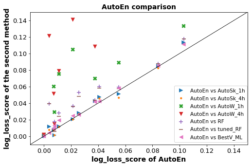
(a) AutoEn

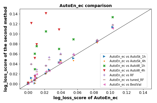
(b) AutoEn_ec

Figure 3: log_loss_score over 12 multi-class datasets. Points above the $y=x$ line correspond to datasets for which our method performs better than a comparison algorithm

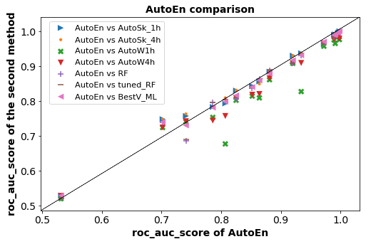
(a) AutoEn

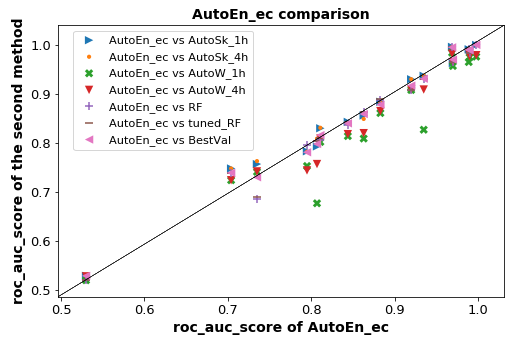
(b) AutoEn_ec

Figure 4: roc_auc_score over 16 binary datasets. Points below the $y=x$ line correspond to datasets for which our method performs better than a comparison algorithm

Similarly, Figures 3a and 3b compare AutoEn and AutoEn_ec to a second method in multi-class datasets. Note that log_loss_score is a minimisation metric; therefore, points above y=x are datasets wherein AutoEn and AutoEn_ec have a higher performance than a second method. For this latter case, the values are normalised between 0 and 1, and outliers were discarded. The reason to normalise the values is that, as was shown in Table 5, there are multi-class problems wherein some methods obtained values greater than 1.

In a general way, it can be observed for binary datasets, AutoEn and AutoEn_ec have in the majority of the cases similar results to the comparison methods. On the other hand, in multi-class problems, our two approaches have a performance generally better than the other methods.

Finally, as the computational cost is also a relevant factor in AutoML, Figure 5 shows the execution time per fold that AutoEn took to make classifications on binary datasets. The Figure also plots the execution time of its economy mode. Figure 5 also has straight lines that represent the time thresholds of the two optimisation execution times associated with Auto-sklearn and Auto-WEKA. Thus, the purpose is to check whether the execution times of AutoEn can be in-between, below or beyond these two thresholds.

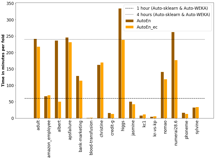
Figure 5: AutoEn execution times in binary datasets under its default and economy modes

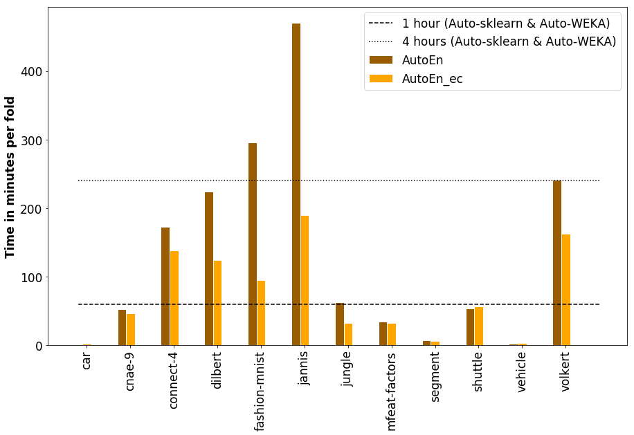
Figure 6: AutoEn execution times in multi-class datasets under its default and economy modes

In Figure 5, the execution time of AutoEn in its default mode has three different behaviours. First, in blood-transfusion, credit-g, jasmine, kc1, kr-vs-kp, phoneme and sylvine datasets, AutoEn spends less than 60 minutes per fold that is the shortest execution time allocated for Auto-sklearn and Auto-WEKA. Secondly, for adult, amazon_employee, albert, bank-marketing, christine and nomao datasets, its execution time is in-between the the two thresholds. Finally, for the remaining datasets (apsfailure, higgs, numerai28.6), AutoEn takes more than 4 hours of time. With resgard to AutoEn_ec, its execution time is below 4 hours in all binary datasets, and as it was observed in Figure 4b, its performance remains quite similar to AutoEn.

Figure 6 summarises AutoEn and AutoEn_ec execution times per fold of in multi-class datasets. Besides, it also shows the 2 time thresholds of the two optimisation execution times carried out by Auto-sklearn and Auto-WEKA. Significant reductions of time can be seen in dilbert, fashion-mnist, jannis and volkert datasets, without affecting the performance as was observed in Figure 3b.

5.2 Results in Traffic Forecasting

This section presents and analyses the results obtained by AutoEn in TF. Specifically, we aim to compare the competitiveness and the significance of AutoEn with regard to a general-purpose AutoML method (Auto-sklearn) that is state-of-the-art in TF problems.

Table 8 shows the mean $log\_loss\_score$ values of our AutoML method, the AutoML competitors (AutoSk_15m, AutoSk_60m, AutoSk_150m), and the baseline methods on the test phase. The best result for each dataset is highlighted in bold-face, and note that the lower the loss value (log_loss), the better. Observing Table 8, we can point out the following:

Table 8: Mean $log\_loss$ (values obtained by AutoEn, the three ET of Auto-sklearn and the two baseline methods. Values highlighted in bold are the highest performance obtained by any of the methods on every dataset

Type	dataset	AutoEn	AutoSk_15m	AutoSk_60m	AutoSk_150m	BestV_ML	RF
Freeway	T_CD_5m	0.220	0.229	0.225	0.223	0.244	0.233
	T_CD_15m	0.340	0.360	0.346	0.348	0.371	0.366
	T_CD_30m	0.381	0.398	0.389	0.391	0.417	0.442
	T_CD_45m	0.393	0.438	0.429	0.420	0.439	0.472
	T_CD_60m	0.401	0.499	0.454	0.453	0.424	0.489
	TS_CD_5m	0.128	0.117	0.114	0.116	0.142	0.133
	TS_CD_15m	0.166	0.163	0.164	0.169	0.187	0.185
	TS_CD_30m	0.186	0.193	0.192	0.197	0.212	0.218
	TS_CD_45m	0.180	0.195	0.182	0.182	0.199	0.217
	TS_CD_60m	0.182	0.218	0.197	0.204	0.185	0.229
Urban	T_CD_15m	0.530	0.502	0.500	0.503	0.537	0.539
	T_CD_30m	0.538	0.516	0.510	0.505	0.536	0.568
	T_CD_45m	0.530	0.513	0.512	0.495	0.537	0.571
	T_CD_60m	0.534	0.508	0.500	0.508	0.553	0.569
	TS_CD_15m	0.406	0.390	0.387	0.389	0.412	0.420
	TS_CD_30m	0.429	0.435	0.434	0.437	0.468	0.461
	TS_CD_45m	0.439	0.447	0.453	0.452	0.494	0.482
	TS_CD_60m	0.435	0.437	0.438	0.437	0.457	0.485
Wins		11	1	4	2	0	0

• As a general overview of results, AutoEn is the most competitive learning approach. This can be seen in the wins distribution as follows: (11) AutoEn, (4) AutoSk_60m, (2) AutoSk_150m, and (1) AutoSk_15m. Moreover, AutoEn and the three ETs of AutoSk are better than RF over all datasets; while they are better than BestV_ML in almost all datasets.

• In freeway datasets, AutoEn is the better approach, especially in time horizons of predictions that range from 30 to 60 minutes in datasets with temporal-spatial (TS) traffic data. On the other hand, AutoEn is the better approach in all datasets that have only temporal (T) traffic data. Besides, AutoSk_15s and AutoSk_60m are more competitive in shorter time horizons (5 and 15 minutes) of freeway datasets with TS traffic data. In this sense, AutoEn achieves to offer competitive results over long-term time horizons that were identified as a drawback of other AutoML approaches in previous resarch [8, 9, 10].

• In urban datasets, AutoEn is more competitive in datasets that contain temporal-spatial (TS) data. Contrary, its performance is just behind Auto-sklearn in datasets with only temporal (T) traffic data.

• As it was previously discussed in results of the general-purpose domain showed in Section 5, longer ETs allocated for the optimisation do not guarantee better performance. This assumption work properly in some datasets (freeway: T_CD_5m, T_CD_45m, T_CD_60m; urban: T_CD_30m, T_CD_45m). However, in some other cases, longer ETs end up with similar results to the ones obtained with shorter ETs (freeway: TS_CD_5m, TS_CD_30m; urban: T_CD_15m, TS_CD_60m); or in the worst of the cases, they tend to decrease the performance of Auto-sklearn (freeway: TS_CD_15m, TS_CD_30m; urban: TS_CD_15m, TS_CD_30m).

To assess whether the differences in performance observed in Table 8 are significant or not, we used the same non-parametric statistical tests mentioned before. Table 9 exposes the test outcomes and the $p$-values lower than 0.05 are shown in bold. In this case, AutoEn is the method in the first position of the ranking. However, it is only statistical better than RF and BestV_ML.

Table 9: Friedman’s average ranking and $p$-values obtained through Holm post-hoc test using AutoEn as control method

Methods	Av. Ranking	$p$-values
AutoEn	2.1667	-
AutoSk_60m	2.3333	0.9520
AutoSk_150m	3.6111	0.9520
AutoSk_15m	3.3333	0.1841
BestV_ML	4.9444	0
RF	5.6111	0

From Tables 9, it is possible to observe that despite the Friedman’s test provides a ranking of the methods evaluated, there were no statistical differences among some of them, particularly between the AutoML methods. Therefore, to better assess the performance, we introduce the following analyses of Figure 7. Each point compares AutoEn to a second method on the multi-class datasets. The x-axis position of the points is the log_loss_score of our method on, while the y-axis position represents the performance metric of the comparison algorithms. Points above the y=x line correspond to datasets for which AutoEn performs better than a second method. From Figure 7 it can be observed that AutoEn has in most of the cases better results than the comparison methods.

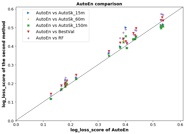
Figure 7: Log loss score over 18 traffic forecasting datasets. Points above the $y=x$ line correspond to datasets for which our method performs better than a comparison algorithm

In summary, AutoEn can overcome the optimisation and meta-learning issues of AutoML in TF. A simple strategy based on the construction of multi-classifiers systems achieves better results in TF problems without pre-defined time budgets for the optimisation process and without being limited by the representativeness of meta-learning. Although AutoSk_60m and AutoSk_150m achieved better results than AutoEn in some particular cases, non-expert ML user must test Auto-sklearn multiple times using different ETs to find these competitive results.

6 Conclusions

In this paper, we introduced AutoEn, a new AutoML method for supervised problems that has a search strategy supported by the construction of ensembles of multiple classifiers. AutoEn was tested against Auto-sklearn and Auto-WEKA, two state-of-the-art AutoML methods, in multiple binary and multi-class supervised problems of a well-established AutoML benchmark, which have been used in TF previously. Besides, we test AutoEn against Auto-sklearn in TF, considering various multi-class TF problems. The main conclusions drawn from the results are:

• AutoEn can be better and more competitive than state-of-the-art AutoML approaches in supervised TF problems. Notably, it is less prone to overfitting than Auto-sklearn because its ensemble strategy makes more robust predictions as multiple classifiers are considered at the same time. Besides, AutoEn can better adapt to different time horizons, specifically, in long-term time horizons that are a crucial element for transportation users when are managing traffic flows.

• Finally, it is relevant to note that in the TF domain, transportation users non-experts in ML could use other AutoML methods focused on optimisation of individual pipelines and achieve satisfactory results. However, as the core of other AutoML strategies is based on optimisation, the user should test multiple times different time budgets to deliver competitive results. This is a task that involves human effort and time costs, which does not have clear guidelines to decide the best ET depending on the size of the dataset at hand. Therefore, AutoEn arises a promising approach that overcomes these limitations while it can supply the demands of non-expert ML users in TF problems.

• Ensembles of multi-classifiers can be more adaptable to datasets of different sizes, which leads to optimising the computational efficiency of AutoML in TF and other problem domains. On the one hand, high-performance solutions can be achieved for small- and medium-size datasets faster than traditional optimisation approaches (e.g., Bayesian optimisation, evolutionary programming). On the contrary, although the time consumption could increase for big datasets, the computation effort of the online phase is focused on finding competitive combinations of multi-classifiers. Moreover, AutoEn’s approach is highly parallelisable compared to generating and fine-tuning individual pipelines that are even more costly to be evaluated in big datasets.

• The online phase of AutoML should be focused on building ensembles rather than individual ML pipelines. Thus, computational effort should be directed to generate high-performance pipelines in the offline period of AutoML, which later contribute to producing competitive and fast ensembles during the online stage of AutoML. These ensembles are less prone to overfitting and are not exposed to the drawbacks of meta-learning and meta-features, as is supported by other general-purpose AutoML methods like Auto-Gluon [26]. Although AutoEn’s ensemble approach can also be optimised, its hyperparameters are a reduced set of values. Such a characteristic of AutoEn constitutes a much less complicated search space compared to the online optimisation of pipelines with a higher degree of hyperparameters.

References

- [1] J. S. Angarita-Zapata, A. D. Masegosa, I. Triguero, A taxonomy of traffic forecasting regression problems from a supervised learning perspective, IEEE Access.
- [2] F. Hutter, L. Kotthoff, J. Vanschoren (Eds.), Automated Machine Learning: Methods, Systems, Challenges, Springer, 2018.
- [3] H. Song, I. Triguero, E. Özcan, A review on the self and dual interactions between machine learning and optimisation, Progress in Artificial Intelligence (2019) 1–23.
- [4] G. Luo, A review of automatic selection methods for machine learning algorithms and hyper-parameter values, Network Modeling Analysis in Health Informatics and Bioinformatics 5 (1) (2016) 18.
- [5] Q. Yao, M. Wang, Y. Chen, W. Dai, H. Yi-Qi, L. Yu-Feng, T. Wei-Wei, Y. Qiang, Y. Yang, Taking Human out of Learning Applications: A Survey on Automated Machine Learning, CoRR.
- [6] M.-A. Zöller, M. F. Huber, Survey on Automated Machine Learning, arXiv preprint arXiv:1904.12054arXiv:1904.12054.
-
[7]
E. I. Vlahogianni,
Optimization
of traffic forecasting: Intelligent surrogate modeling, Transportation
Research Part C: Emerging Technologies 55 (2015) 14 – 23, engineering and
Applied Sciences Optimization (OPT-i) - Professor Matthew G. Karlaftis
Memorial Issue.
URL http://www.sciencedirect.com/science/article/pii/S0968090X15000959 - [8] J. S. Angarita-Zapata, I. Triguero, A. D. Masegosa, A preliminary study on automatic algorithm selection for short-term traffic forecasting, in: J. Del Ser, E. Osaba, M. N. Bilbao, J. J. Sanchez-Medina, M. Vecchio, X.-S. Yang (Eds.), Intelligent Distributed Computing XII, Springer International Publishing, Cham, 2018, pp. 204–214.
- [9] J. S. Angarita-Zapata, A. D. Masegosa, I. Triguero, General-purpose automated machine learning for transportation: A case study of auto-sklearn for traffic forecasting, in: Proceeding of the 18th International Conference on Information Processing and Management of Uncertainty in Knowledge-Based Systems, Springer International Publishing, Cham, 2020.
- [10] J. S. Angarita-Zapata, A. D. Masegosa, I. Triguero, Evaluating Automated Machine Learning on Supervised Regression Traffic Forecasting Problems, Springer International Publishing, Cham, 2020, pp. 187–204.
- [11] C. Thornton, F. Hutter, H. H. Hoos, K. Leyton-Brown, Auto-weka: Combined selection and hyperparameter optimization of classification algorithms, in: Proceedings of the 19th International Conference on Knowledge Discovery and Data Mining, Association for Computing Machinery, 2013, p. 847–855.
- [12] M. Feurer, A. Klein, K. Eggensperger, J. Springenberg, M. Blum, F. Hutter, Efficient and Robust Automated Machine Learning, in: C. Cortes, N. D. Lawrence, D. D. Lee, M. Sugiyama, R. Garnett (Eds.), Advances in Neural Information Processing Systems, Curran Associates, Inc., 2015, pp. 2962–2970.
- [13] P. Gijsbers, E. LeDell, S. Poirier, J. Thomas, B. Bischl, J. Vanschoren, An open source automl benchmark, CoRRWork presented at AutoML Workshop at International Conference on Machine Learning 2019.
- [14] M. Galar, A. Fernandez, E. Barrenechea, H. Bustince, F. Herrera, An overview of ensemble methods for binary classifiers in multi-class problems: Experimental study on one-vs-one and one-vs-all schemes, Pattern Recognition 44 (8) (2011) 1761 – 1776.
- [15] C. M. Bishop, Pattern Recognition and Machine Learning (Information Science and Statistics), Springer-Verlag, Berlin, Heidelberg, 2006.
- [16] S. Garcia, J. Luengo, F. Herrera, Data preprocessing in data mining, Springer. Cham, Switzerland, 2015.
- [17] I. Triguero, D. García-Gil, J. Maillo, J. Luengo, S. García, F. Herrera, Transforming big data into smart data: An insight on the use of the k-nearest neighbors algorithm to obtain quality data, Wiley Interdisciplinary Reviews: Data Mining and Knowledge Discovery 9 (2) (2019) e1289.
- [18] J. M. Kanter, K. Veeramachaneni, Deep feature synthesis: Towards automating data science endeavors, in: 2015 IEEE International Conference on Data Science and Advanced Analytics, 2015, pp. 1–10.
- [19] G. Katz, E. C. R. Shin, D. Song, Explorekit: Automatic feature generation and selection, in: 2016 IEEE 16th International Conference on Data Mining, 2016, pp. 979–984.
- [20] F. Nargesian, H. Samulowitz, U. Khurana, E. B. Khalil, D. Turaga, Learning feature engineering for classification, in: Proceedings of the 26th International Joint Conference on Artificial Intelligence, AAAI Press, 2017, pp. 2529–2535.
- [21] J. Bergstra, R. Bardenet, Y. Bengio, B. Kégl, Algorithms for hyper-parameter optimization, in: Proceedings of the 24th International Conference on Neural Information Processing Systems, Curran Associates Inc., USA, 2011, pp. 2546–2554.
- [22] F. Hutter, H. H. Hoos, K. Leyton-Brown, Sequential Model-Based Optimization for General Algorithm Configuration, in: C. A. C. Coello (Ed.), Learning and Intelligent Optimization, Springer Berlin Heidelberg, Berlin, Heidelberg, 2011, pp. 507–523.
- [23] M. Claesen, J. Simm, D. Popovic, Y. Moreau, B. D. Moor, Easy hyperparameter search using optunity, CoRR.
- [24] R. S. Olson, N. Bartley, R. J. Urbanowicz, J. H. Moore, Evaluation of a Tree-based Pipeline Optimization Tool for Automating Data Science, in: Proceedings of the Genetic and Evolutionary Computation Conference 2016, 2016, pp. 485–492.
- [25] J. Vanschoren, Meta-learning, in: Hutter et al. [2], pp. 39–68.
- [26] N. Erickson, J. Mueller, A. Shirkov, H. Zhang, P. Larroy, M. Li, A. Smola, Autogluon-tabular: Robust and accurate automl for structured data, arXiv preprint arXiv:2003.06505.
- [27] R. Caruana, A. Niculescu-Mizil, G. Crew, A. Ksikes, Ensemble selection from libraries of models, in: Proceedings of the Twenty-First International Conference on Machine Learning, Association for Computing Machinery, New York, NY, USA, 2004, p. 18.
- [28] I. Guyon, I. Chaabane, H. J. Escalante, S. Escalera, D. Jajetic, J. R. Lloyd, N. Macià, B. Ray, L. Romaszko, M. Sebag, A. R. Statnikov, S. Treguer, E. Viegas, A brief review of the chalearn automl challenge: Any-time any-dataset learning without human intervention, in: Proceedings of the Workshop on Automatic Machine Learning, PMLR, New York, USA, 2016, pp. 21–30.
- [29] B. Bischl, G. Casalicchio, M. Feurer, F. Hutter, M. Lang, R. G. Mantovani, J. N. van Rijn, J. Vanschoren, Openml benchmarking suites (2017). arXiv:1708.03731.
- [30] J. Vanschoren, J. N. van Rijn, B. Bischl, L. Torgo, Openml: Networked science in machine learning, SIGKDD Explor. Newsl. 15 (2) (2014) 49–60.
- [31] I. B. M. Skycomp, Major High- way Performance Ratings and Bottleneck Inventory, Maryland State Highway Administration, the Baltimore Metropolitan Council and Maryland Transportation Authority, State of Maryland, 2009.
- [32] S. Garcia, A. Fernandez, J. Luengo, F. Herrera, Advanced nonparametric tests for multiple comparisons in the design of experiments in computational intelligence and data mining: Experimental analysis of power, Information Sciences 180 (10) (2010) 2044 – 2064.
- [33] S. Falkner, A. Klein, F. Hutter, Bohb: Robust and efficient hyperparameter optimization at scale, CoRR.