Anderson Impurities In Edge States with Nonlinear Dispersion

Abstract

A non-linear dispersion can significantly impact the Kondo problem, resulting in anomalous effects on electronic transport. By analyzing a special bath with a $\theta=\frac{\pi}{3}$ symmetry rotation in the Brillouin zone or 3-fold symmetry in momentum, we derive an effective spin-spin interacting model. Combining the anisotropic Dzyaloshinskii-Moriya (DM) interaction with non-linear dispersion can lead to exceptional points $(E_{p})$ in a Hermitian model. Our RG analysis reveals that the spin relaxation time has the signature of coalescence in momentum-resolved couplings and an ideal logarithmic divergence in resistivity over a range of nonlinearity ($\beta$). The effective model at the impurity subspace has a Lie group structure of Dirac matrices. We show nontrivial renormalization within a Poorman approximation with the inclusion of potential scattering, and the invariant obtained will not be altered by potential scattering. We expand the model to a two-impurity Kondo model and investigate the Kondo destruction and anomalous spin transport signature by calculating the spin-relaxation time ($\tau$).Analysis of RG equations zeros and poles show a ”Sign Reversion”(SR) regime exists for a Hermitian problem with a critical value of nonlinear coupling $J_{k^{3}}$. Our results show the existence of an out-of-phase RKKY oscillation above and below the critical value of the chemical potential.

I Introduction

The occurrence of the Kondo peak and bound states in Topological Insulators[1, 2] (TIs) highly depends on various parameters such as topology and chemical potential. The behavior of the resonance level is distinct from that of simple metals and ordinary insulators. In the case of band inversion[3], the mixed-valence regime is wider, and the coexistence of both the Kondo peak and in-gap bound states is possible, unlike in ordinary insulators where only one exists. If the impurity energy is far from the chemical potential, the in-gap bound states merge into the bulk. Furthermore, a self-screening Kondo effect may occur due to the interaction between the impurity and the bound-state spin. The study[4] predicts the occurrence of quantized conductance in the presence of strong disorder, even in parameters where the system is a metal in the absence of disorder. Unlike previously studied topological insulators, the Fermi energy is located within a mobility gap, and the existence of ballistic edge states does not rely on band inversion. Further investigation is necessary to determine the correlation between the presence of strong disorder and the location of the topological Anderson insulator in the phase diagram.

The analysis presented in the study[5] investigates the impact of an Anderson impurity on a 2D topological insulator. It demonstrates that the exchange interaction between the impurity and an in-gap bound state can undergo dynamic changes. The temperature dependence of the system exhibits crossover behavior, which could provide experimental evidence for the theoretical analysis. In the weak-coupling regime, both screened and underscreened Kondo effects display a modification in their effective coupling constant as a function of temperature. The interplay between topology and interactions[6] was analyzed; analysis shows an interesting relationship between topology and interactions. The critical strength for the interaction is smaller in situations where the total charge of the system does not change during a transition. The critical strength also does not change with a change in the system’s topology. The rearrangement of the charge structure in the ordered phases can be studied through spectroscopy or optical response measurements. Further studies of the relationship between interactions and topology can provide new insights.

The effect of thermal bias on the two-impurity Kondo system was studied[7]. Findings show that Kondo correlations are destroyed for large thermal bias for the dot connected to the hot reservoir. This leads to suppressed electrical and heat flows as the dots get decoupled. Kondo correlations also influence the interdot coupling. For non-negligible antiferromagnetic spin exchange coupling, thermal bias affects the Kondo-to-AFM crossover. The critical value for the crossover increases as thermal bias increases. These observations can be experimentally tested due to advancements in thermoelectrical transport through nanostructures. This work is also important for some engineered nanostructures for thermoelectric systems.

The study of Two Impurity Models (TIK)[8, 9, 10, 11, 12, 13, 14, 15, 16, 17, 18, 19, 20] has previously focused on a variety of regimes, including over-screened and unscreened phases, as well as impurity triplet and decoupled single dot states. Unlike the single impurity case, TIK presents a complex problem with numerous possible configurations and interactions between impurities. These models have been studied extensively to understand the interplay between magnetic interactions, Kondo physics, and electronic transport properties in complex systems.

The article[21] examines the effects of Kondo screening and its interplay with scalar disorder on transport properties in Weyl semimetals, leading to Weyl-Kondo physics. At zero temperature, magnetic impurities generate a Kondo resistivity that scales with the number of impurities. At finite temperatures, the strength of the scalar disorder impacts the Kondo resistivity. In the case of weak scalar disorder, the Kondo resistivity has a minimum, but it may not be observed in strong disorder, even if part of the sample is Kondo screened.
We start with a generic model for the bath, which is well-considered for the Topological Insulators(TI)[22, 6, 23].By projecting onto the singly-occupied subspace of the dot, we obtain an effective Hamiltonian, which is an s-d exchange model. We show its lie algebra and connection to conformal field theory (CFT), and it’s topological properties. Later we also extend the projected model to a two impurities case which will be a two-impurity kondo model in a topological system. We performed two-loop RG calculations for one impurity and one-loop for the TIK model within the Poorman scaling approximations. We analytically and numerically solved the RG equations, found invariants, and explored rich phase diagram of the problem. We highlight transport signatures relevant for momentum-resolved measurements of the impurity-bath systems.

II Formalism

We start with the proposed and studied model[22] in the context of topological insulators. This was used to explicitly extract the bulk and surface contributions from the model perspective. The model reads as the following,

$$\begin{split}\hat{H}&=\alpha k^{2}_{\parallel}.\mathbb{I}+\beta k^{3}_{\parallel}\cos(3\theta)\sigma_{z}+\hat{z}.(\vec{k}\times\vec{\sigma})\end{split}$$ (1)

Where in the above we have $\vec{k}=k_{x}\hat{i}+k_{y}\hat{j}+k_{z}\hat{k}$ and $\vec{\sigma}=\sigma_{x}\hat{i}+\sigma_{y}\hat{j}+\sigma_{z}\hat{k}$ This model in the eqn 1 is well studied in the context of topology with such a nonlinear dispersion; the term spin coupling to momentum is studied in the many body context by introducing spin-orbit coupling. We write the above in the second quantized form for spinful fermions as the following,

$$\begin{split}H&=\psi^{\dagger}\hat{H}\psi\end{split}$$ (2)

In the above model, the basis vector $\psi^{\dagger}=\begin{pmatrix}c^{\dagger}_{k\uparrow}&c^{\dagger}_{k\downarrow}\end{pmatrix}$.Now we put an impurity with onsite interaction and hybridization with the edge states Hamiltonian as the following,

$$H_{siam}=\psi^{\dagger}\hat{H}\psi+H_{d}+\sum_{k\sigma}V_{k}(c^{\dagger}_{k\sigma}d_{\sigma}+hc)$$ (3)

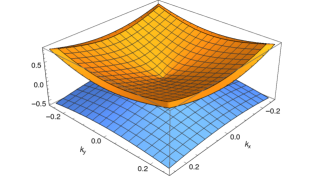
Figure 1: The band dispersion around the low k points from diagonalization of the bath represents the emergent chiral bands.In this case we set $\beta=0.3$ and $\theta=\frac{\pi}{3}$ we observed more $\beta$ was flattening the bands.

Where in above single impurity model equation 3 $H_{d}=\sum_{\sigma}\epsilon_{d}d^{\dagger}_{\sigma}d_{\sigma}+Un_{d\uparrow}n_{d\downarrow}$ in the bath Hamiltonian we can replace the $k_{\parallel}$ with $k$ with a parametrization $k_{x}\pm ik_{y}=k_{\parallel}e^{\pm i\theta}$.We do a unitary operation which is k-dependent in bath operators preserving canonical relations, which yields a nonlinear k dependent coefficients as the following,

$$\begin{split}\mathcal{U}=\frac{1}{\sqrt{\mathcal{N}}}\begin{pmatrix}e^{i\frac{\theta}{2}}\alpha_{k1}&e^{-i\frac{\theta}{2}}\alpha_{k2}\\ -ie^{i\frac{\theta}{2}}\alpha_{k2}&ie^{-i\frac{\theta}{2}}\alpha_{k1}\end{pmatrix}\end{split}$$ (4)

In the above equation 4, we have $\alpha_{1}=\sqrt{\frac{\Delta}{2}+\beta k^{3}\cos 3\theta}$ and $\alpha_{2}=\sqrt{\beta k^{3}\cos 3\theta-\frac{\Delta}{2}}$, where $\Delta=\sqrt{4\beta^{2}k^{6}\cos^{2}3\theta+4k^{2}}$, and the normalization constant is given by $\mathcal{N}=\sqrt{|\alpha_{1}|^{2}+|\alpha_{2}|^{2}}$.

This unitary transformation will rotate the original bath operators as $\tilde{\psi}_{k}=\mathcal{U}_{k}\psi_{k}$, and such a k-dependent operation is possible as shown in the case of weyl multiplicity[24], which is also a different form of nonlinear dispersion. An interesting work also discusses weyl-like signatures in quasiparticle interference[25] in the different forms of cubic dispersive $(k_{x}\pm ik_{y})^{3}$ baths. Also note that the expression $\sqrt{\beta k^{3}\cos 3\theta-\frac{\Delta}{2}}=-i\sqrt{\frac{\Delta}{2}-\beta k^{3}\cos 3\theta}$ is also a unitary operator. The reason for choosing this particular form is that it leads to a simpler normalization constant for the unitary, which makes subsequent analysis easier.

$$\begin{split}\tilde{\psi}&=\begin{pmatrix}c_{k+}\\ c_{k-}\end{pmatrix}=\mathcal{U}\psi\\ c_{k+}&=\frac{1}{\sqrt{\beta k^{3}\cos 3\theta}}\bigg{(}e^{i\frac{\theta}{2}}\sqrt{\frac{\Delta}{2}+\beta k^{3}\cos 3\theta}c_{k\uparrow}\\ &+e^{-i\frac{\theta}{2}}\sqrt{\beta k^{3}\cos 3\theta-\frac{\Delta}{2}}c_{k\downarrow}\bigg{)}\\ c_{k-}&=\frac{1}{\sqrt{\beta k^{3}\cos 3\theta}}\bigg{(}-ie^{i\frac{\theta}{2}}\sqrt{\beta k^{3}\cos 3\theta-\frac{\Delta}{2}}c_{k\uparrow}\\ &+ie^{-i\frac{\theta}{2}}\sqrt{\frac{\Delta}{2}+\beta k^{3}\cos 3\theta}c_{k\downarrow}\bigg{)}\end{split}$$ (5)

Inverting the above unitary operator to express the original spin basis to these new chiral operators,

$$\begin{split}c_{k\uparrow}&=\frac{1}{\sqrt{\beta k^{3}\cos 3\theta}}\bigg{(}e^{-i\frac{\theta}{2}}\sqrt{\frac{\Delta}{2}+\beta k^{3}\cos 3\theta}c_{k+}\\ &+ie^{-i\frac{\theta}{2}}\sqrt{\beta k^{3}\cos 3\theta-\frac{\Delta}{2}}c_{k-}\bigg{)}\\ c_{k\downarrow}&=\frac{1}{\sqrt{\beta k^{3}\cos 3\theta}}\bigg{(}e^{i\frac{\theta}{2}}\sqrt{\beta k^{3}\cos 3\theta-\frac{\Delta}{2}}c_{k+}\\ &-ie^{-i\frac{\theta}{2}}\sqrt{\frac{\Delta}{2}+\beta k^{3}\cos 3\theta}c_{k-}\bigg{)}\end{split}$$ (6)

This will effectively generate a chiral model with the eigenergies as $\epsilon_{\pm}=\alpha k^{2}\pm\frac{1}{2}\Delta$ and the hybridization as the following,

$$\begin{split}\tilde{H}^{+}_{hyb}&=\sum_{k}\tilde{V}_{k}\bigg{(}e^{i\frac{\theta}{2}}\sqrt{\frac{\Delta}{2}+\beta k^{3}\cos 3\theta}c^{\dagger}_{k+}d_{\uparrow}+hc)\\ &+\sum_{k}\tilde{V}_{k}\bigg{(}e^{i\frac{\theta}{2}}\sqrt{\beta k^{3}\cos 3\theta-\frac{\Delta}{2}}c^{\dagger}_{k+}d_{\downarrow}+hc\bigg{)}\\ \tilde{H}^{-}_{hyb}&=\sum_{k}\tilde{V}_{k}\bigg{(}-ie^{i\frac{\theta}{2}}\sqrt{\beta k^{3}\cos 3\theta-\frac{\Delta}{2}}c^{\dagger}_{k-}d_{\uparrow}+hc\bigg{)}\\ &+\sum_{k}\tilde{V}_{k}\bigg{(}ie^{i\frac{\theta}{2}}\sqrt{\frac{\Delta}{2}+\beta k^{3}\cos 3\theta}c^{\dagger}_{k-}d_{\downarrow}+hc\bigg{)}\end{split}$$ (7)

This will create the $\frac{3}{2}$ singularity of momentum in the hybridization as $\tilde{V}_{k}=\frac{V_{k}}{\sqrt{\beta k^{3}\cos 3\theta}}$ distinguishing it from the square root singularity by the Rashba coupling studies[26, 27, 28, 29].In order to simplify the symbolic cumbersome, let’s introduce two k-dependent constants as $\alpha_{k1}=\sqrt{\frac{\Delta}{2}+\beta k^{3}\cos 3\theta}$ and $\alpha_{k2}=\sqrt{\beta k^{3}\cos 3\theta-\frac{\Delta}{2}}$. If we look at the $\theta=\frac{\pi}{3}$ 3-fold rotations might seem that the hybridization has become complex, but it will introduce a phase factor, but overall hybridization remains Hermitian. Hybridization in the new notation appears as follows,

$$\begin{split}\tilde{H}^{+}_{hyb}&=\sum_{k}\tilde{V}_{k}\alpha_{k1}\bigg{(}e^{i\frac{\theta}{2}}c^{\dagger}_{k+}d_{\uparrow}+hc\bigg{)}\\ &+\sum_{k}\tilde{V}_{k}\alpha_{k2}\bigg{(}e^{i\frac{\theta}{2}}c^{\dagger}_{k+}d_{\downarrow}+hc\bigg{)}\\ \tilde{H}^{-}_{hyb}&=\sum_{k}\tilde{V}_{k}\alpha_{k2}\bigg{(}-ie^{i\frac{\theta}{2}}c^{\dagger}_{k-}d_{\uparrow}+hc\bigg{)}\\ &+\sum_{k}\tilde{V}_{k}\alpha_{k1}\bigg{(}ie^{i\frac{\theta}{2}}c^{\dagger}_{k-}d_{\downarrow}+hc\bigg{)}\end{split}$$ (8)

We project this model to impurity subspace using the standard Hewson’s projection operator method. The projection operators are $P_{0}=(1-n_{\uparrow})(1-n_{\downarrow})$, $P_{1}=n_{\uparrow}(1-n_{\downarrow})+n_{\downarrow}(1-n_{\uparrow})$ and $P_{2}=n_{\uparrow}n_{\downarrow}$, respectively, for unoccupied, singly occupied and doubly occupied states. We employ the projections and write the following components of the effective model,

$$\begin{split}\tilde{H}^{+}_{10}&=\sum_{k}\tilde{V}_{k}\alpha_{k1}e^{-i\frac{\theta}{2}}d^{\dagger}_{\uparrow}(1-n_{\downarrow})c_{k+}\\ &+\sum_{k}e^{-i\frac{\theta}{2}}\tilde{V}_{k}\alpha_{k2}d^{\dagger}_{\downarrow}(1-n_{\uparrow})c_{k+}\\ \tilde{H}^{-}_{10}&=\sum_{k}i\tilde{V}_{k}\alpha_{k2}e^{-i\frac{\theta}{2}}d^{\dagger}_{\uparrow}(1-n_{\downarrow})c_{k-}\\ &+\sum_{k}-ie^{-i\frac{\theta}{2}}\tilde{V}_{k}\alpha_{k1}d^{\dagger}_{\downarrow}(1-n_{\uparrow})c_{k-}\end{split}$$ (9)

Similarly, we have the projections connecting doubly and singly occupied space. The $H_{02}$ and $H_{20}$ will vanish. $H_{12}$ can be written for this form of hybridization,

$$\begin{split}\tilde{H}^{+}_{12}&=\sum_{k}\tilde{V}_{k}\alpha_{k1}e^{i\frac{\theta}{2}}c^{\dagger}_{k+}d_{\uparrow}n_{\downarrow}+\sum_{k}e^{i\frac{\theta}{2}}\tilde{V}_{k}\alpha_{k2}c^{\dagger}_{k+}d_{\downarrow}n_{\uparrow}\\ \tilde{H}^{-}_{12}&=-\sum_{k}i\tilde{V}_{k}\alpha_{k2}e^{i\frac{\theta}{2}}c^{\dagger}_{k-}d_{\uparrow}n_{\downarrow}+\sum_{k}ie^{i\frac{\theta}{2}}\tilde{V}_{k}\alpha_{k1}c^{\dagger}_{k-}d_{\downarrow}n_{\uparrow}\end{split}$$ (10)

Remaining components are $H_{00}=\sum_{k\alpha}\epsilon_{k\alpha}c^{\dagger}_{k\alpha}c_{k\alpha}P_{0}+\sum_{\sigma}\epsilon_{d}n_{\sigma}P_{0}$ and $H_{22}=\sum_{k\alpha}\epsilon_{k\alpha}c^{\dagger}_{k\alpha}c_{k\alpha}P_{2}+\sum_{\sigma}\epsilon_{d}n_{\sigma}P_{2}+Un_{\uparrow}n_{\downarrow}P_{2}$. Now we have all the components to calculate the effective models in various sub-spaces.

$$\begin{split}H^{0}_{eff}&=H_{00}+\bigg{(}\sum_{\alpha}H^{\alpha}_{01}\bigg{)}\frac{1}{E-H_{11}}\bigg{(}\sum_{\alpha}H^{\alpha}_{10}\bigg{)}\\ H^{1}_{eff}&=H_{11}+\bigg{(}\sum_{\alpha}H^{\alpha}_{10}\bigg{)}\frac{1}{E-H_{00}}\bigg{(}\sum_{\alpha}H^{\alpha}_{01}\bigg{)}\\ &+\bigg{(}\sum_{\alpha}H^{\alpha}_{12}\bigg{)}\frac{1}{E-H_{22}}\bigg{(}\sum_{\alpha}H^{\alpha}_{21}\bigg{)}\\ H^{2}_{eff}&=H_{22}+\bigg{(}\sum_{\alpha}H^{\alpha}_{21}\bigg{)}\frac{1}{E-H_{11}}\bigg{(}\sum_{\alpha}H^{\alpha}_{12}\bigg{)}\end{split}$$ (11)

The singly occupied subspace is the low-energy effective model for the Kondo regime. We want to explore the non-Kondo regime Hamiltonian to explore the operator structures in the later sections. We detail the calculations in the appendix for an effective sd exchange model.

$$\begin{split}H^{1}_{eff}=H_{0}-i\alpha^{2}_{1}M_{kk^{\prime}}S_{-}s^{+}_{kk^{\prime}}+i\alpha^{2}_{2}M_{kk^{\prime}}s^{-}_{kk^{\prime}}S_{+}\\ \alpha^{2}_{1}M_{kk^{\prime}}S_{z}s^{z}_{kk^{\prime}}+\alpha^{2}_{2}M_{kk^{\prime}}s^{z}_{kk^{\prime}}S_{z}\\ \alpha_{1}\alpha_{2}M_{kk^{\prime}}S_{-}s^{z}_{kk^{\prime}}+\alpha_{1}\alpha_{2}M_{kk^{\prime}}s^{z}_{kk^{\prime}}S_{+}\\ i\alpha_{1}\alpha_{2}M_{kk^{\prime}}S_{z}s^{-}_{kk^{\prime}}-i\alpha_{1}\alpha_{2}M_{kk^{\prime}}s^{+}_{kk^{\prime}}S_{z}\end{split}$$ (12)

In above equation 12 $M_{kk^{\prime}}=\tilde{V}_{k}\tilde{V}_{k^{\prime}}\bigg{(}\frac{1}{\epsilon_{k^{\prime}}-\epsilon_{d}}+\frac{1}{\epsilon_{d}+U-\epsilon_{k}}\bigg{)}$ The above spin-spin interaction model has an algebraic structure similar to the CFT paper[30]. We can notice some cross-product terms pop out in such a nonlinear dispersion similar to the $\mathcal{DM}$ interaction term[26] for the chiral channel but in the spin basis of the bath operators;

$$\begin{split}H^{1}_{eff}&=H_{0}+\sum_{kk^{\prime}}J_{0}S.s_{kk^{\prime}}+i\sum_{kk^{\prime}}\vec{J}_{k^{3}}.(S\times s_{kk^{\prime}})\\ &+i\sum_{kk^{\prime}}\vec{J}_{k}.(S\times s_{kk^{\prime}})+H_{pot}\end{split}$$ (13)

where in the above $\vec{J}_{k^{3}}=\frac{M^{\theta}_{k}}{\beta k^{3}\cos 3\theta}\Delta\hat{z}$ and $\vec{J}_{k}=\frac{kM}{\beta k^{3}\cos 3\theta}\hat{x}+\frac{k\Delta}{\beta k^{3}\cos 3\theta}M^{\theta}\hat{y}$ Also, $H^{\dagger}=H$ since $\alpha_{1,2}$ are real constants and in the limit $\Delta\to 0$, we have a standard hermitian problem with Anderson impurity in a bath. Note that in this limit model no longer has anisotropic$\mathcal{DM}$interaction. The band electrons’ left and right mover can be defined and shown in the figure 2 for the above model. After Poorman scaling is done for the magnitude of the vectors as defined in the equ 13, we collect the contributions for RG equations in terms of these magnitudes.

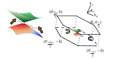
Figure 2: A schematic representing two Anderson impurities in edge states. We separate the left and right scatterers with green and blue arrows.$k_{\parallel}\to k$ and $\theta\to\tan^{-1}\frac{k_{y}}{k_{x}}$ see derivation. Scatterings for the $(k,\theta)$ to $(-k,\theta^{\prime})$ in Poorman scaling are represented schematically in a 3D shell.

$$\begin{split}\frac{dJ_{0}}{dl}&=J^{2}_{0}+J_{k^{3}}J_{k}+J^{2}_{k^{3}}+J^{2}_{k}\\ \frac{dJ_{k^{3}}}{dl}&=J^{2}_{k}+J_{0}J_{k^{3}}\\ \frac{dJ_{k}}{dl}&=J_{0}J_{k}\end{split}$$ (14)

One solution of the above RG equations $J^{2}_{k}-J_{k}=mJ_{k^{3}}$ where m is an invariant and remaining solution, we detail the analytic solution in the appendix.

III Emergence Of Complex Solution

Notably, the emergence of complex solutions to RG equations due to nonlinear dispersion has nontrivial renormalization. This is also seen in the one-loop Poorman equations, which yield the emergent exceptional point scenario [30, 31] as RG reversion. Moreover, adding second-order self-energy to the original Hamiltonian leads to non-Hermitian physics [32]. In open systems, adding finite-order self-energies can also give rise to effective non-Hermitian models [33, 34, 35]. In a theoretical study, it has been shown that complex solutions emerge from various types of potentials and their symmetries [36].

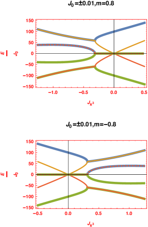
Figure 3: The above plots show the emergence of coalescing point inside the fermi-level. These points are solely due to the renormalization of the linear and nonlinear couplings in the spin sector(1,1). Where m is RG invariant which arises from the one loop poorman scaling.

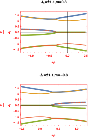
Figure 4: The above plots show the spin sector(1,1) eigenvalues for large $J_{0}>1.0$. The eigenvalues become flatter as the bare coupling increases, but coalescence remains, but it only disappears for $J_{0}\to\infty$

Based on the plots in Figures 3 and 4, one might conclude that the Dirac cone has disappeared, but in reality, it still exists in the bath. We are only visualizing the eigenvalues of the sd model, which is more relevant to impurity and dirac cone exist3 for resonant level case, which depend on the flown couplings. The spectrum becomes gapped in impurity in large $J_{0}$ limit. By substituting the RG invariant $J_{k}=\frac{1}{2}\pm\frac{1}{2}\sqrt{1+4mJ_{k^{3}}}$ into the sd model eigenvalues, we see that this is the source of the coalescing points. Interestingly, these points disappear in the limit of $J_{0}\to\infty$. To examine the relevance of potential scattering and its effect on particle-hole symmetry, we diagonalize the flown $H^{1}_{eff}$ at the single occupancy sector for only the sd part. In real materials, analogous exceptional points have been observed, and in calculations, they have been tuned [37, 38]. Thus, finite nonlinear dispersion can generate a complex solution and significantly modify the RG flow of the Kondo problem, as shown by the Poorman solution.

IV Renormalization With Potential Scattering

To study the various momentum channel scattering shown in figure 2, which interestingly yields rich physics. Largely we can write the effective model derived13 with scattering terms as follows,

$$\begin{split}(H^{\prime})^{1}_{eff}&=H^{1}_{eff}+\\ &\begin{pmatrix}[k,\theta_{+2\frac{\pi}{3}}]\Leftrightarrow[k,\theta_{+\frac{\pi}{3}}]&[k,\theta_{+2\frac{\pi}{3}}]\Leftrightarrow[-k,\theta_{-\frac{\pi}{3}}]\\ [-k,\theta_{-2\frac{\pi}{3}}]\Leftrightarrow[k,\theta_{+\frac{\pi}{3}}]&[-k,\theta_{-2\frac{\pi}{3}}]\Leftrightarrow[-k,\theta_{-\frac{\pi}{3}}]\end{pmatrix}\end{split}$$ (15)

As discussed above, we can rewrite the effective Hamiltonian considering such a potential scattering. We consider the basis of bath in the new scattering as $\psi^{\dagger}=\begin{pmatrix}c^{\dagger}_{k_{\theta_{\frac{2\pi}{3}}}+},&c^{\dagger}_{k_{\theta_{\frac{\pi}{3}}}-},&c^{\dagger}_{-k_{\theta_{-\frac{2\pi}{3}}}+},&c^{\dagger}_{-k_{\theta_{-\frac{\pi}{3}}}-}\end{pmatrix}$ which makes the block structure of the kondo problem and represents the couplings $\vec{J}^{\theta,\theta^{\prime}}_{k^{3}}=M^{\theta,\theta^{\prime}}_{kk^{\prime}}(\Delta+\beta k^{3}\cos(3\theta))\hat{z}$ and $\vec{J}^{\theta,\theta^{\prime}}_{k}=\frac{k}{\beta k^{3}\cos 3\theta}M^{\theta,\theta^{\prime}}\hat{x}+\frac{k\Delta}{\beta k^{3}\cos 3\theta}M^{\theta,\theta^{\prime}}\hat{y}$

$$\begin{split}H^{1}_{eff}&=H_{0}+\sum_{kk^{\prime}}J_{0}S.\psi^{\dagger}(\Sigma)\psi\\ &+i\sum_{kk^{\prime}}\vec{J}^{(0,0)}_{k^{3}}.(S\times\psi^{\dagger}(\Sigma)\psi)\\ &-\sum_{kk^{\prime}}\vec{J}^{\theta_{\pm\frac{2\pi}{3}},\theta_{\pm\frac{\pi}{3}}}_{k^{3}}.(S\times\psi^{\dagger}(\Omega)\psi)\\ &+\sum_{kk^{\prime}}\vec{J}^{\theta_{\frac{2\pi}{3}},\theta_{-\frac{\pi}{3}}}_{k^{3}}.(S\times\psi^{\dagger}(\Gamma)\psi)\\ &+i\sum_{kk^{\prime}}\vec{J}^{(0,0)}_{k}.(S\times\psi^{\dagger}(\Sigma)\psi)\\ &-\sum_{kk^{\prime}}\vec{J}^{\theta_{\pm\frac{2\pi}{3}},\theta_{\pm\frac{\pi}{3}}}_{k}.(S\times\psi^{\dagger}(\Omega)\psi)\\ &+i\sum_{kk^{\prime}}\vec{J}^{\theta_{\frac{2\pi}{3}},\theta_{-\frac{\pi}{3}}}_{k}.(S\times\psi^{\dagger}(\Gamma)\psi)\end{split}$$ (16)

IV.1 Comparison With CFT scaling laws at two loops

We can see the algebraic consistency in the earlier works [30, 8, 39] using the lie algebra of matrices, which is similar to the Poorman scaling for the operator structures but CFT will be exact since it incorporates the bath states more accurately. This idea can also be extended to the two impurity problems. After introducing the potential scattering, we have a more general model16 in the lie matrices, which are defined as follows,

$$\begin{split}\Sigma=\begin{pmatrix}\sigma&\sigma\\ \sigma&\sigma\end{pmatrix},\Omega=\begin{pmatrix}\sigma&0\\ 0&-\sigma\end{pmatrix},\Gamma=\begin{pmatrix}\sigma&0\\ 0&\sigma\end{pmatrix}\end{split}$$ (17)

where in the above equation17 $\sigma$ are the Pauli matrices

$$\begin{split}[\Sigma^{a}\Sigma^{b},\Sigma^{c}]&=[\Gamma^{a}\Gamma^{b},\Gamma^{c}]=[\Omega^{a}\Omega^{b},\Omega^{c}]\\ &=0\\ [\Sigma^{\alpha}\Sigma^{\alpha^{\prime}},\Sigma^{\alpha}]&=-4i\delta_{\alpha,\alpha^{\prime}}\Sigma^{\alpha}\\ [\Sigma^{b}\Sigma^{b},\Sigma^{c}]&=\Sigma^{b}[\Sigma^{b},\Sigma^{c}]+[\Sigma^{b},\Sigma^{c}]\Sigma^{b}\\ &=+8i\epsilon^{abc}\Sigma^{c}\\ [\Omega^{b}\Omega^{b},\Omega^{c}]&=\Omega^{b}[\Omega^{b},\Omega^{c}]+[\Omega^{b},\Omega^{c}]\Omega^{b}\\ &=+4i\epsilon^{abc}\Omega^{c}\\ [\Omega^{b}\Omega^{b},\Sigma^{c}]&=\Omega^{b}[\Omega^{b},\Sigma^{c}]+[\Omega^{b},\Sigma^{c}]\Omega^{b}\\ &=+4i\epsilon^{abc}\Omega^{c}+4i\epsilon^{abc}\mathit{I}_{4X4}\\ [\Sigma^{a}\Sigma^{b},\Upsilon]&=\Sigma^{a}[\Sigma^{b},\Upsilon]+[\Sigma^{a},\Upsilon]\Sigma^{b}\\ &=0\end{split}$$ (18)

$$\begin{split}\frac{dJ_{0}}{dl}&=J^{2}_{0}+J^{2}_{k^{3}}+J^{2}_{k}+J_{k^{3}}J_{k}+J^{2}_{k}J_{0}+J^{2}_{k^{3}}J_{0}+J^{3}_{0}\\ &+f(J_{k^{3}},g_{2k},g_{2k^{3}},J_{k})\\ \frac{dJ_{k^{3}}}{dl}&=J^{2}_{k}+J_{0}J_{k^{3}}+J^{2}_{k}J_{k^{3}}+J^{2}_{0}J_{k^{3}}+J^{3}_{k^{3}}\\ \frac{dJ_{k}}{dl}&=J_{0}J_{k}+J^{2}_{0}J_{k}+J_{k}J^{2}_{k^{3}}+J^{3}_{k}\\ \frac{dg_{1k^{3}}}{dl}&=g^{3}_{1k^{3}}-g^{2}_{1k}g_{1k^{3}}\\ \frac{dg_{1k}}{dl}&=g^{3}_{1k}-g^{2}_{1k^{2}}g_{1k}\\ \frac{dg_{2k^{3}}}{dl}&=-g^{3}_{2k^{3}}+g^{2}_{1k^{3}}g_{2k^{3}}\\ \frac{dg_{2k}}{dl}&=-g^{3}_{2k}+g^{2}_{1k}g_{2k}\end{split}$$ (19)

We have given some details on calculations of the above rg equations in Appendix B.

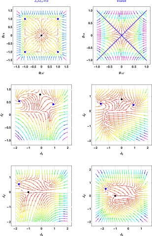
Figure 5: We set $g_{1k}=g_{1k^{3}}=1$ which is invariant derived in appendix for all calculations $J_{1k}=\frac{1}{2}\pm\frac{1}{2}\sqrt{1+4mJ_{1k^{3}}}$ is used and $m=-4$ we set for all above plots.We plot the grid as $\begin{pmatrix}pot&pot1\\ R^{+}R^{+}&R^{+}I^{+}\\ I^{-}R^{-}&I^{-}I^{-}\end{pmatrix}$ first row is potential scattering, and the second row is in both beta functions chosen real and imaginary part of the positive root. We see at least two fixed points(FP), two spirals in (RR, RI) row, and one spiral, and one is marginal. The dotted lines in the second plot of the first row are a family of FP’s.

The spiral FP in non-hermitian systems are demonstrated earlier[40, 41]; also, in three and higher dimensions, spiral invariants obtained[42]. We explored the FP originating from the invariant by adding the potential scattering terms. This made the problem richer and interestingly captured the one-loop critical points discussed in analytic solutions to RG eq’s in the appendix and didn’t alter the invariant of poorman. This indicates the additional terms are very relevant for the problem, unlike in a homogeneous bath at particle-hole symmetry, these potential scattering terms are irrelevant (note that potential scattering terms are conventional $k\neq k^{\prime}$, not special like what is considered here). In general, $\vec{S}\times\vec{s}$ terms are anti-hermitian without the factor $\iota$; hence any finite order perturbation will bring nonhermitian physics into play; in general, it does come into play as a decohering interaction[43]. Various experiments relating to anisotropic $\mathcal{DM}$ and topology of the spin texture[44] are discussed. We detail the numerical solutions in Appendix G for confirming the ’sign reversion’. If so, these points correspond to complex FP, independent of what potential scattering terms we add.

V Generalization to Two Impurities

We generalize this model to two impurity kondo models with coupling between the impurities. One can also start with the projection for two impurities Anderson models to derive the two impurity kondo model from getting exact matrix elements for coupling between the dots. Two dots with spin-orbit coupling[45] is studied earlier, which shows that $\mathcal{DM}$ term exists for only Y-component and linear dispersion in the bath. In this case, it generates a more general form of $S_{1}\times S_{2}$ term in all components.

$$\begin{split}H^{1}_{eff}&=H_{0}+\sum_{kk^{\prime}}J_{0}S_{\alpha}.s_{kk^{\prime}}+i\sum_{kk^{\prime}\alpha}\vec{J}_{k^{3}}.(S_{\alpha}\times s_{kk^{\prime}})\\ &+i\sum_{kk^{\prime}\alpha}\vec{J}_{k}.(S_{\alpha}\times s_{kk^{\prime}})+H_{pot}\\ &+J_{Y}S_{1}.S_{2}+iK.(S_{1}\times S_{2})\end{split}$$ (20)

With the new coupling, we see how it renormalizes the problem; immediately, we can notice that the RKKY coupling $J_{Y}$ modifies the single impurity invariant. Since the generalized problem has many coupling, we restrict our-self to analyzing the one-loop RG equations.,

$$\begin{split}\frac{dJ_{0}}{dl}&=J^{2}_{0}+J_{k^{3}}J_{k}+J^{2}_{k^{3}}+J^{2}_{k}+J_{Y}J_{0}+KJ_{0}\\ \frac{dJ_{k^{3}}}{dl}&=J^{2}_{k}+J_{0}J_{k^{3}}+J_{Y}J_{k^{3}}+J_{Y}J_{k}+KJ_{k^{3}}\\ \frac{dJ_{k}}{dl}&=J_{0}J_{k}+J_{Y}J_{k^{3}}+J_{Y}J_{k}+KJ_{k}\\ \frac{dJ_{Y}}{dl}&=J^{2}_{Y}+K^{2}+J^{2}_{0}+J_{k^{3}}J_{k}+J^{2}_{k}+J^{2}_{k^{3}}\\ \frac{dK}{dl}&=K^{2}+KJ_{Y}+J_{k^{3}}J_{k}\end{split}$$ (21)

Solutions to the above equations are detailed in an appendix in various limits. The beta function zeros for kondo destruction can be seen in the odd-even couplings given in articles[46, 47]. Since we focus on the nonlinear couplings $J_{k},J_{k^{3}}$, We look at the solutions around the anomalous contributions to Spin-relaxation time and the FP’s in these couplings.

V.1 Kondo Scale in two Impurity

We integrate the RG equations to get the scales for the problem in various limits so that how the nonlinear coupling affects this problem. First in limit $J_{k^{3}}=J_{k}=K=0$ we have the solution $J_{0}=\frac{e^{-g}}{(1-g)^{2}}$ by integrating the $J_{0},J_{Y}$ equations, where $g=\frac{J_{Y}}{J_{0}}$. We solve when impurity $\mathcal{DM}$ interaction $K\neq 0$ in the appendix in two limits which does not have a straightforward analytic solution by reducing to bergurs equation . Figure 6 show the variation of $T_{K}$ with various coupling limits. The two invariants $R_{1}$ modify the TIK problem significantly, ”R” cause the destruction of the TIK bound state, and $R_{1}$ try to stabilize the bound state, which can be seen in the middle plot in figure 6. A special bath can significantly affect the kondo problem, as shown in NRG studies in single impurity[48]. Recent NRG studies[49, 50] on two impurities anderson model yield a rich phase like kondo, local moment valence fluctuation, RKKY, and spin liquid. Since we employed perturbative renormalization, the flow will cuttoff and we need to go beyond; hence we don’t have access to all phases, however we do have Kondo-RKKY phases in small K limit inset fig 6 and qualitative physical picture of phases in homogeneous bath cases.Now we solve the set of coupled equations21 numerically for various IC’s found in flow diagrams and analytic solutions.

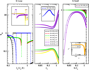
Figure 6: We plot the scales, as shown above, to show competition between RKKY and impurity$\mathcal{DM}$ interactions.An Inset graph in K small label is an analytic expression derived when impurity $\mathcal{DM}$ interaction is absent and $g=\frac{J_{Y}}{J_{0}}$ in the x-axis. Discontinuity in the scale for K Large limit is shown with the dotted line where it is ill-defined.

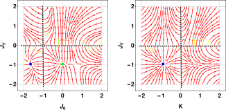
Figure 7: RG flows for the two impurity problems when anisotropic $\mathcal{DM}$ interaction due to bath is absent. See the RG solutions in the appendix. There are three FP’s from these solutions one is TIK point(blue), decoupled dots(Green), and dot triplet state(blue in the right plot). The quadrant of these points depends on the integral constants(either in third or first), and we refer here to the $-ve$ sign for ferromagnetic couplings.

VI RG Equations Zeros And Poles Analysis

We realize that the solutions to couplings are divergent; therefore, it becomes trickier to separate the two impurity kondo regime, single impurity kondo regime, and the SR regime of couplings due to nonlinear coupling $J_{k^{3}}$. We solve the RG ODE’s by allowing complex solutions and analyzing solutions around the FP’s found in flow diagrams. If there is a phase transition, then couplings will flow to a stable FP, and hence we should see poles in functions and at unstable points only zero crossings. This serves as the numerical diagnosis for the identification of various phases.

VII Impurity Transport Calculation

We have derived the anomalous contributions for the relaxation time in the appendix due to the presence of the nonlinear dispersive bath following the $\mathcal{T}_{kk^{\prime}}$ formalism[51] which is detailed in appendix F,

$$\begin{split}\frac{1}{\tau(k)}\propto(1-2J\tilde{g}_{\alpha}(\epsilon_{k})-2J\tilde{g}_{\alpha}^{*}(\epsilon_{k})-2J_{k^{3}}\tilde{g}_{\alpha k^{3}}(\epsilon_{k})\\ -2J_{k^{3}}\tilde{g}_{\alpha k^{3}}^{*}(\epsilon_{k})-2J_{k}\tilde{g}_{\alpha k}(\epsilon_{k})-2J_{k}\tilde{g}_{\alpha k}^{*}(\epsilon_{k}))\end{split}$$ (22)

We are addressing coalescing points from a hermitian model with any transport signature. The appendix evaluates these functions as contour integrals for polar components and definite integrals for radial fermi vector($k_{f}$). Spin relaxation time will reflect the RG invariant as $\frac{1}{\tau}\propto\tilde{g}_{\epsilon}=(1\pm\sqrt{1+4\epsilon})f(\epsilon,\epsilon^{\prime})$ implying the momentum resolved couplings have the signature of coalescing points which can be seen in spin relaxation time.

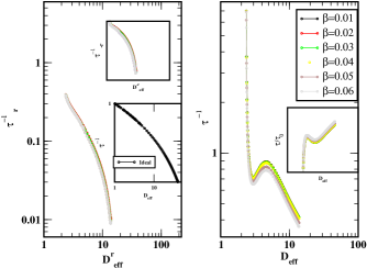
Figure 8: We calculated the spin-relaxation time to see the coalescing point signature with the nonlinear coupling $\beta$. as the $\beta$ decreases, ideal log divergence reaches but dips persist in $\frac{1}{\tau}$. Left plot to confirm if the anomalous contribution is from the coalescence, we divided each curve by lowest $\beta=0.01$ curve and scaled for $\pm$ roots as $\tau^{-1}_{\pm r}=\tau^{-1}*(1\pm\sqrt{4(\epsilon-0.25)+1})$ for the y-axis and $D_{eff}*(1\pm\sqrt{4(\epsilon-0.25)+1})$ for the x-axis. Increasing $\beta$, we see polynomial contributions dominate; hence the scaling will be absent.

The matrix elements scale as $M_{kk^{\prime}}\approx\frac{1}{\sqrt{k^{3}\cos(3\theta)}\sqrt{(k^{\prime})^{3}\cos{3\theta^{\prime}}}}$ and when $k=-k^{\prime}$ there is an imaginary coupling which creates a non-Hermitian Kondo problem with a bath that has non-linear dispersion. Various studies of non-Hermitian Kondo systems exist, considering different perspectives, symmetry considerations, and complex spin exchange interactions[31, 30, 52, 53]. In the presence of inversion symmetry, non-Hermiticity can result from $\theta^{\prime}\to\frac{\pi}{3}-\theta$, where a Dirac point exists in the Brillouin zone. In the appendix, it is discussed that $\alpha_{1k}\alpha_{2k^{\prime}}$ beyond the poor man’s limit (i.e., $k\neq k^{\prime}$) results in a general non-Hermitian model at impurity due to nonlinear parametric dispersion in the bath.

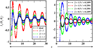
Figure 9: We perform The integrals for $J_{Y}$ given in the appendix and plot by varying the bandwidth.RKKY is enhanced for $\beta<1.0$ and approaches to ideal flatt band limit for $\beta>1.0$. As we saw in the relaxation time here, we can see above and below a critical value of chemical potential ($\epsilon^{\prime}=\pm 0.25$), $J^{odd}_{Y}$ reverses sign and goes out of phase in $J^{odd}_{Y}$.The other channel $J^{even}_{Y}$ has standard RKKY oscillations and decay amplify around the EP.

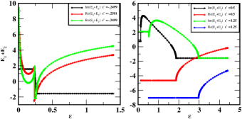
Figure 10: We plot the elliptic functions which arose in calculating the RKKY integrals. For negative chemical potential $\epsilon^{\prime}$, there is SR everywhere else we see the exceptional point behaviors. The EP’s start shifting for increasing +ve $\epsilon^{\prime}$, but there is no SR in the real part of these special functions. This odd channel shows EP or SR behavior which is relevant in RG when dominant odd channel scattering will emerge complex FP’s in such models.

VIII Discussion

This work investigates the possibility of coalescing points in a bulk system having magnetic impurities through spin relaxation time calculations in different momentum directions. Our results show that two distinct calculations share a common invariant as renormalization group (RG) solutions, with or without potential scattering. Increasing nonlinearity strength causes bands to flatten in the bath spectrum while the impurity resistivity reaches the ideal log divergence for a $\beta$ strength range. Furthermore, we analyze RG calculations on single and two impurity problems in a homogeneous bath. The competition between RKKY and Kondo interactions is only observed when the impurity $\mathcal{DM}$-interaction is absent. We also show that to obtain coalescing points in hermitian Kondo models, anisotropic $\mathcal{DM}$ interactions are necessary due to the $k^{3}$ and $k$ terms in the dispersion, which naturally yields the roots as the RG invariants. These results are significant as they provide a signature in transport, which we demonstrate through numerical diagnosis for critical values of $J_{k^{3}}$ and $J_{k}$ in the couplings, confirmed by flow diagrams. The SR regime in the couplings corresponds to the spiral FP’s of the problem. Out-Of-Phase oscillations in the RKKY in the odd channels are due to the presence of the special bath, as we ruled out the other possibilities by analyzing the elliptic functions EP. Future work could extend these findings to charge and thermal transport calculations and investigate impurity effects in systems with anisotropic $\mathcal{DM}$ interaction and in Weyl and topological systems with nonlinear dispersion. One may expect a loss of unitarity in subsystem as we have seen here in a single occupied subspace if we analyze the system in other subspaces $H^{0}_{eff},H^{2}_{eff}$ maybe there will be global unitarity which is not done in current work.

The results of our work demonstrate the potential for more advanced numerical techniques, such as the Numerical Renormalization Group (NRG), to extract valuable information about spin transport in complex systems. This opens up new avenues for future research to investigate the behavior of impurities in systems with anisotropic $\mathcal{DM}$ interactions and in Weyl and topological systems with nonlinear dispersion.It is important to note that we did not explore charge or thermal transport in our study. These are interesting directions for future research, as they could provide a more complete understanding of the transport properties of impurities in topological systems. Nonhermitian problems can also originate from certain defects[54, 55], and different boundary conditions can be used to tune[56] the EP’s and realize them in quantum circuits, maybe if we map effective spin models to Wilson chains, then we might look at these phases. Localization in the Hatano-nelson type of models can have dramatic consequences of impurities[57]. Our work contributes to a growing body of research to better understand impurities’ behavior in topological systems. This can inform the design of new materials and devices with enhanced transport properties and deepen our fundamental understanding of phenomena associated with open and closed condensed matter systems.

Appendix A Projection details for deriving effective sd model

$$\begin{split}\tilde{H}^{+}_{12}&=\sum_{k}\tilde{V}_{k}\alpha_{k1}e^{i\frac{\theta}{2}}c^{\dagger}_{k+}d_{\uparrow}n_{\downarrow}+\sum_{k}e^{i\frac{\theta}{2}}\tilde{V}_{k}\alpha_{k2}c^{\dagger}_{k+}d_{\downarrow}n_{\uparrow}\\ \tilde{H}^{-}_{12}&=-\sum_{k}i\tilde{V}_{k}\alpha_{k2}e^{i\frac{\theta}{2}}c^{\dagger}_{k-}d_{\uparrow}n_{\downarrow}+\sum_{k}ie^{i\frac{\theta}{2}}\tilde{V}_{k}\alpha_{k1}c^{\dagger}_{k-}d_{\downarrow}n_{\uparrow}\end{split}$$ (23)

We will derive the components of hamiltonian as done in the text[51] as follows,

$$\begin{split}H^{+}_{12}\frac{1}{E-H_{22}}H^{+}_{21}+H^{+}_{12}\frac{1}{E-H_{22}}H^{-}_{21}+H^{-}_{12}\frac{1}{E-H_{22}}H^{+}_{21}+H^{-}_{12}\frac{1}{E-H_{22}}H^{-}_{21}\\ \bigg{(}\sum_{k}\tilde{V}_{k}\alpha_{k1}e^{i\frac{\theta}{2}}c^{\dagger}_{k+}d_{\uparrow}n_{\downarrow}+\sum_{k}e^{i\frac{\theta}{2}}\tilde{V}_{k}\alpha_{k2}c^{\dagger}_{k+}d_{\downarrow}n_{\uparrow}\bigg{)}^{\dagger}\frac{1}{E-H_{22}}\bigg{(}\sum_{k^{\prime}}\tilde{V}_{k^{\prime}}\alpha_{k^{\prime}1}e^{i\frac{\theta^{\prime}}{2}}c^{\dagger}_{k^{\prime}+}d_{\uparrow}n_{\downarrow}+\sum_{k^{\prime}}e^{i\frac{\theta^{\prime}}{2}}\tilde{V}_{k^{\prime}}\alpha_{k^{\prime}2}c^{\dagger}_{k^{\prime}+}d_{\downarrow}n_{\uparrow}\bigg{)}\\ \bigg{(}\sum_{k}\tilde{V}_{k}\alpha_{k1}e^{i\frac{\theta}{2}}c^{\dagger}_{k+}d_{\uparrow}n_{\downarrow}+\sum_{k}e^{i\frac{\theta}{2}}\tilde{V}_{k}\alpha_{k2}c^{\dagger}_{k+}d_{\downarrow}n_{\uparrow}\bigg{)}^{\dagger}\frac{1}{E-H_{22}}\bigg{(}-\sum_{k^{\prime}}i\tilde{V}_{k^{\prime}}\alpha_{k^{\prime}2}e^{i\frac{\theta^{\prime}}{2}}c^{\dagger}_{k^{\prime}-}d_{\uparrow}n_{\downarrow}+\sum_{k^{\prime}}ie^{i\frac{\theta}{2}}\tilde{V}_{k^{\prime}}\alpha_{k^{\prime}1}c^{\dagger}_{k^{\prime}-}d_{\downarrow}n_{\uparrow}\bigg{)}\\ \bigg{(}-\sum_{k}i\tilde{V}_{k}\alpha_{k2}e^{i\frac{\theta}{2}}c^{\dagger}_{k-}d_{\uparrow}n_{\downarrow}+\sum_{k}ie^{i\frac{\theta}{2}}\tilde{V}_{k}\alpha_{k1}c^{\dagger}_{k-}d_{\downarrow}n_{\uparrow}\bigg{)}^{\dagger}\frac{1}{E-H_{22}}\bigg{(}\sum_{k^{\prime}}\tilde{V}_{k^{\prime}}\alpha_{k^{\prime}1}e^{i\frac{\theta^{\prime}}{2}}c^{\dagger}_{k^{\prime}+}d_{\uparrow}n_{\downarrow}+\sum_{k^{\prime}}e^{i\frac{\theta^{\prime}}{2}}\tilde{V}_{k^{\prime}}\alpha_{k^{\prime}2}c^{\dagger}_{k^{\prime}+}d_{\downarrow}n_{\uparrow}\bigg{)}\\ \bigg{(}-\sum_{k}i\tilde{V}_{k}\alpha_{k2}e^{i\frac{\theta}{2}}c^{\dagger}_{k-}d_{\uparrow}n_{\downarrow}+\sum_{k}ie^{i\frac{\theta}{2}}\tilde{V}_{k}\alpha_{k1}c^{\dagger}_{k-}d_{\downarrow}n_{\uparrow}\bigg{)}^{\dagger}\frac{1}{E-H_{22}}\bigg{(}-\sum_{k^{\prime}}i\tilde{V}_{k^{\prime}}\alpha_{k^{\prime}2}e^{i\frac{\theta^{\prime}}{2}}c^{\dagger}_{k^{\prime}-}d_{\uparrow}n_{\downarrow}+\sum_{k^{\prime}}ie^{i\frac{\theta^{\prime}}{2}}\tilde{V}_{k^{\prime}}\alpha_{k^{\prime}1}c^{\dagger}_{k^{\prime}-}d_{\downarrow}n_{\uparrow}\bigg{)}\end{split}$$ (24)

We calculate for the $\theta=\theta^{\prime}$ cases, and the remaining can be included in potential scattering later.

$$\begin{split}&\sum_{k}M^{22}_{k+}\alpha^{2}_{k1}n_{\downarrow}d^{\dagger}_{\uparrow}c_{k+}c^{\dagger}_{k+}d_{\uparrow}n_{\downarrow}+\sum_{k}M^{22}_{k+}\alpha_{k2}\alpha_{k1}n_{\uparrow}d^{\dagger}_{\downarrow}c_{k+}c^{\dagger}_{k+}d_{\uparrow}n_{\downarrow}\\ &+\sum_{k}M^{22}_{k+}\alpha_{k1}\alpha_{k2}n_{\downarrow}d^{\dagger}_{\uparrow}c_{k+}c^{\dagger}_{k+}d_{\uparrow}n_{\uparrow}+\sum_{k}M^{22}_{k+}\alpha^{2}_{k2}n_{\uparrow}d^{\dagger}_{\downarrow}c_{k+}c^{\dagger}_{k+}d_{\downarrow}n_{\uparrow}\\ &i\sum_{k}M^{22}_{k-}\alpha^{2}_{k1}n_{\downarrow}d^{\dagger}_{\uparrow}c_{k+}c^{\dagger}_{k-}d_{\downarrow}n_{\uparrow}-i\sum_{k}M^{22}_{k-}\alpha_{k2}\alpha_{k1}n_{\downarrow}d^{\dagger}_{\uparrow}c_{k+}c^{\dagger}_{k-}d_{\uparrow}n_{\downarrow}\\ &+i\sum_{k}M^{22}_{k-}\alpha_{k1}\alpha_{k2}n_{\downarrow}d^{\dagger}_{\uparrow}c_{k+}c^{\dagger}_{k-}d_{\downarrow}n_{\uparrow}-i\sum_{k}M^{22}_{k-}\alpha^{2}_{k2}n_{\uparrow}d^{\dagger}_{\downarrow}c_{k+}c^{\dagger}_{k-}d_{\uparrow}n_{\downarrow}\\ &-i\sum_{k}M^{22}_{k+}\alpha^{2}_{k1}n_{\uparrow}d^{\dagger}_{\downarrow}c_{k-}c^{\dagger}_{k+}d_{\uparrow}n_{\downarrow}+i\sum_{k}M^{22}_{k+}\alpha_{k2}\alpha_{k1}n_{\downarrow}d^{\dagger}_{\uparrow}c_{k-}c^{\dagger}_{k+}d_{\uparrow}n_{\downarrow}\\ &-i\sum_{k}M^{22}_{k+}\alpha_{k1}\alpha_{k2}n_{\uparrow}d^{\dagger}_{\downarrow}c_{k-}c^{\dagger}_{k+}d_{\downarrow}n_{\uparrow}+i\sum_{k}M^{22}_{k+}\alpha^{2}_{k2}n_{\downarrow}d^{\dagger}_{\uparrow}c_{k-}c^{\dagger}_{k+}d_{\downarrow}n_{\uparrow}\\ &\sum_{k}M^{22}_{k-}\alpha^{2}_{k1}n_{\uparrow}d^{\dagger}_{\downarrow}c_{k-}c^{\dagger}_{k-}d_{\downarrow}n_{\uparrow}-\sum_{k}M^{22}_{k-}\alpha_{k2}\alpha_{k1}n_{\uparrow}d^{\dagger}_{\downarrow}c_{k-}c^{\dagger}_{k-}d_{\uparrow}n_{\downarrow}\\ &-\sum_{k}M^{22}_{k-}\alpha_{k1}\alpha_{k2}n_{\downarrow}d^{\dagger}_{\uparrow}c_{k-}c^{\dagger}_{k-}d_{\downarrow}n_{\uparrow}+\sum_{k}M^{22}_{k-}\alpha^{2}_{k2}n_{\downarrow}d^{\dagger}_{\uparrow}c_{k-}c^{\dagger}_{k-}d_{\uparrow}n_{\downarrow}+(k\neq k^{\prime}\text{terms})\end{split}$$ (25)

Where in above $M^{22}_{k\alpha}=\frac{\tilde{V}^{2}_{k}}{\epsilon_{d}+U-\epsilon_{k^{\prime}\alpha}}\approx M^{22}_{k}(1-\alpha\Delta)$ with this substitution we can seperate the original kondo model and kondo model from the edge states impurity interaction.Collecting terms with $\alpha^{2}_{k1},\alpha^{2}_{2},\alpha_{k1}\alpha_{k2}$ terms and with simplifications using the commutation and some substitution at half filling $n^{2}_{\sigma}=n_{\sigma}$, $n_{\uparrow}\to(\frac{1}{2}-n_{\downarrow})$, $n_{\downarrow}\to(\frac{1}{2}-n_{\uparrow})$ and the dot operators $n_{\sigma}d_{\sigma}=d_{\sigma}(1-n_{\sigma})$ can be written as follows,

$$\begin{split}(\alpha^{2}_{k1})\longrightarrow\sum_{k}M^{22}_{k-}\alpha^{2}_{k1}d^{\dagger}_{\downarrow}c_{k-}c^{\dagger}_{k-}d_{\downarrow}n_{\uparrow}-i\sum_{k}M^{22}_{k+}\alpha^{2}_{k1}n_{\uparrow}d^{\dagger}_{\downarrow}c_{k-}c^{\dagger}_{k+}d_{\uparrow}n_{\downarrow}\\ i\sum_{k}M^{22}_{k-}\alpha^{2}_{k1}n_{\downarrow}d^{\dagger}_{\uparrow}c_{k+}c^{\dagger}_{k-}d_{\downarrow}n_{\uparrow}+\sum_{k}M^{22}_{k+}\alpha^{2}_{k1}d^{\dagger}_{\uparrow}c_{k+}c^{\dagger}_{k+}d_{\uparrow}n_{\downarrow}\\ =\sum_{k}M^{22}_{k}\alpha^{2}_{k1}S^{z}_{d}s^{z}_{kk^{\prime}}-i\sum_{k}M^{22}_{k}\alpha^{2}_{k1}S^{-}s^{+}_{kk^{\prime}}+i\sum_{k}M^{22}_{k}\alpha^{2}_{k1}s^{-}_{kk^{\prime}}S^{+}+(c^{\dagger}_{k\alpha}c_{k\bar{\alpha}}n_{\uparrow}n_{\downarrow}\text{terms})\\ i\sum_{k}M^{22}_{k}\Delta\alpha^{2}_{k1}S^{-}s^{+}_{kk^{\prime}}-i\sum_{k}M^{22}_{k}\Delta\alpha^{2}_{k1}s^{-}_{kk^{\prime}}S^{+}\end{split}$$ (26)

Note that The edge contribution is only appearing in the cross terms does not contribute to $S^{z}_{d}s^{z}_{kk^{\prime}}$.Similarly for $\alpha^{2}_{k2}$ terms

$$\begin{split}(\alpha^{2}_{k2})\longrightarrow\sum_{k}M^{22}_{k+}\alpha^{2}_{k2}n_{\uparrow}d^{\dagger}_{\downarrow}c_{k+}c^{\dagger}_{k+}d_{\downarrow}n_{\uparrow}-i\sum_{k}M^{22}_{k-}\alpha^{2}_{k2}n_{\uparrow}d^{\dagger}_{\downarrow}c_{k+}c^{\dagger}_{k-}d_{\uparrow}n_{\downarrow}\\ +i\sum_{k}M^{22}_{k+}\alpha^{2}_{k2}n_{\downarrow}d^{\dagger}_{\uparrow}c_{k-}c^{\dagger}_{k+}d_{\downarrow}n_{\uparrow}+\sum_{k}M^{22}_{k-}\alpha^{2}_{k2}n_{\downarrow}d^{\dagger}_{\uparrow}c_{k-}c^{\dagger}_{k-}d_{\uparrow}n_{\downarrow}\\ =\sum_{k}M^{22}_{k}\alpha^{2}_{k2}S^{z}_{d}s^{z}_{kk^{\prime}}-i\sum_{k}M^{22}_{k}\alpha^{2}_{k2}S^{-}s^{+}_{kk^{\prime}}+i\sum_{k}M^{22}_{k}\alpha^{2}_{k2}s^{-}_{kk^{\prime}}S^{+}+(c^{\dagger}_{k\alpha}c_{k\bar{\alpha}}n_{\uparrow}n_{\downarrow}\text{terms})\\ i\sum_{k}M^{22}_{k}\Delta\alpha^{2}_{k2}S^{-}s^{+}_{kk^{\prime}}-i\sum_{k}M^{22}_{k}\Delta\alpha^{2}_{k2}s^{-}_{kk^{\prime}}S^{+}\end{split}$$ (27)

Finally we can collect all terms with $\alpha_{1}\alpha_{2}$

$$\begin{split}(\alpha_{k1}\alpha_{k2})\longrightarrow\sum_{k}M^{22}_{k+}\alpha_{k2}\alpha_{k1}n_{\uparrow}d^{\dagger}_{\downarrow}c_{k+}c^{\dagger}_{k+}d_{\uparrow}n_{\downarrow}+\sum_{k}M^{22}_{k+}\alpha_{k1}\alpha_{k2}n_{\downarrow}d^{\dagger}_{\uparrow}c_{k+}c^{\dagger}_{k+}d_{\downarrow}n_{\uparrow}\\ -i\sum_{k}M^{22}_{k-}\alpha_{k2}\alpha_{k1}n_{\downarrow}d^{\dagger}_{\uparrow}c_{k+}c^{\dagger}_{k-}d_{\uparrow}n_{\downarrow}+i\sum_{k}M^{22}_{k-}\alpha_{k1}\alpha_{k2}n_{\uparrow}d^{\dagger}_{\downarrow}c_{k+}c^{\dagger}_{k-}d_{\downarrow}n_{\uparrow}\\ +i\sum_{k}M^{22}_{k+}\alpha_{k2}\alpha_{k1}n_{\downarrow}d^{\dagger}_{\uparrow}c_{k-}c^{\dagger}_{k+}d_{\uparrow}n_{\downarrow}-i\sum_{k}M^{22}_{k+}\alpha_{k2}\alpha_{k1}n_{\uparrow}d^{\dagger}_{\downarrow}c_{k-}c^{\dagger}_{k+}d_{\downarrow}n_{\uparrow}\\ -\sum_{k}M^{22}_{k-}\alpha_{k1}\alpha_{k2}n_{\downarrow}d^{\dagger}_{\uparrow}c_{k-}c^{\dagger}_{k-}d_{\downarrow}n_{\uparrow}-\sum_{k}M^{22}_{k-}\alpha_{k1}\alpha_{k2}n_{\uparrow}d^{\dagger}_{\downarrow}c_{k-}c^{\dagger}_{k-}d_{\uparrow}n_{\downarrow}\end{split}$$ (28)

We simplify the above and use the Abrikosov representation[58] for spin for impurity as $S=\psi^{\dagger}_{d}\sigma\psi_{d}$ and $s_{kk^{\prime}}=\psi^{\dagger}_{k}\sigma\psi_{k^{\prime}}$ for bath operators. Where in the representation $\sigma$ is pauli matrix and $\psi^{\dagger}_{d}=\begin{pmatrix}d^{\dagger}_{\uparrow}&d^{\dagger}_{\downarrow}\end{pmatrix}$ $\psi^{\dagger}_{k}=\begin{pmatrix}c^{\dagger}_{k\uparrow}&c^{\dagger}_{k^{\prime}\downarrow}\end{pmatrix}$

$$\begin{split}i\sum_{k}M^{22}_{k}\alpha_{k2}\alpha_{k1}(-s^{-}_{kk^{\prime}}S^{z}+S^{z}s^{+}_{kk^{\prime}})+\sum_{k}M^{22}_{k}\alpha_{k2}\alpha_{k1}(s^{z}_{kk^{\prime}}S^{+}-S^{-}s^{z}_{kk^{\prime}})\\ +i\sum_{k}M^{22}_{k}\Delta\alpha_{k2}\alpha_{k1}(s^{-}_{kk^{\prime}}S^{z}-S^{z}s^{+}_{kk^{\prime}})-\sum_{k}M^{22}_{k}\Delta\alpha_{k2}\alpha_{k1}(s^{z}_{kk^{\prime}}S^{+}-S^{-}s^{z}_{kk^{\prime}})\end{split}$$ (29)

Similarly we can calculate $H^{+}_{10}\frac{1}{E-H_{00}}H^{+}_{01}+H^{+}_{10}\frac{1}{E-H_{00}}H^{-}_{01}+H^{-}_{10}\frac{1}{E-H_{00}}H^{+}_{01}+H^{-}_{10}\frac{1}{E-H_{00}}H^{-}_{01}$ which yield same operator structure except we have $M^{00}_{k}$ Now substituting back $\alpha_{1}=\sqrt{\frac{\Delta}{2}+\beta k^{3}\cos 3\theta}$ and $\alpha_{2}=\sqrt{\beta k^{3}\cos 3\theta-\frac{\Delta}{2}}$, where $\Delta=\sqrt{4\beta^{2}k^{6}\cos^{2}3\theta+4k^{2}}$ and $\tilde{V}_{k}=\frac{V_{k}}{\sqrt{k^{3}\cos{3\theta}}}$, collecting terms we get various simplifications for example $\alpha^{2}_{k1}+\alpha^{2}_{k2}=\beta k^{3}\cos(3\theta)$ and $\alpha_{k1}\alpha_{k2}=k$

$$\begin{split}H^{1}_{eff}=H_{11}+\beta k^{3}\cos{3\theta}\bigg{(}\sum_{k}M_{k}S^{z}_{d}s^{z}_{kk^{\prime}}-i\sum_{k}M_{k}S^{-}s^{+}_{kk^{\prime}}+i\sum_{k}M_{k}s^{-}_{kk^{\prime}}S^{+}\\ i\sum_{k}M_{k}\Delta S^{-}s^{+}_{kk^{\prime}}-i\sum_{k}M_{k}\Delta s^{-}_{kk^{\prime}}S^{+}\bigg{)}\\ k\bigg{(}i\sum_{k}M_{k}(-s^{-}_{kk^{\prime}}S^{z}+S^{z}s^{+}_{kk^{\prime}})+\sum_{k}M_{k}(s^{z}_{kk^{\prime}}S^{+}-S^{-}s^{z}_{kk^{\prime}})\\ +i\sum_{k}M_{k}\Delta(s^{-}_{kk^{\prime}}S^{z}-S^{z}s^{+}_{kk^{\prime}})-\sum_{k}M_{k}\Delta(s^{z}_{kk^{\prime}}S^{+}-S^{-}s^{z}_{kk^{\prime}})\bigg{)}\end{split}$$ (30)

Collecting All terms from equations 26,27and 29 we can simplify and rewrite the derived effective model as,

$$\begin{split}H^{1}_{eff}&=H_{11}+\sum_{kk^{\prime}}J_{0}S.s_{kk^{\prime}}+i\sum_{kk^{\prime}}\Delta(S\times s_{kk^{\prime}})_{z}+\sum_{kk^{\prime}}i\frac{k}{\beta k^{3}\cos 3\theta}M_{kk^{\prime}}.(S\times s_{kk^{\prime}})_{y}+\sum_{kk^{\prime}}i\frac{k}{\beta k^{3}\cos 3\theta}\Delta M_{kk^{\prime}}.(S\times s_{kk^{\prime}})_{x}\\ \therefore H^{1}_{eff}&=H_{11}+\sum_{kk^{\prime}}J_{0}S.s_{kk^{\prime}}+i\sum_{kk^{\prime}}\vec{J}_{k^{3}}.(S\times s_{kk^{\prime}})+i\sum_{kk^{\prime}}\vec{J}_{k}.(S\times s_{kk^{\prime}})\end{split}$$ (31)

Appendix B Including the potential scattering

The effective model indicates that the matrix elements are scaled as $M^{\theta,\theta^{\prime}}_{kk^{\prime}}\propto\frac{V{k}}{\sqrt{k^{3}\cos 3\theta}}\frac{V_{k^{\prime}}}{\sqrt{k^{\prime 3}\cos 3\theta^{\prime}}}$.If we go beyond poorman’s limit $k=k^{\prime}=k_{f}$ then this leads to four possible potential scattering scenarios: $\vec{J}^{\theta_{\pm\frac{2\pi}{3}},\theta_{\pm\frac{\pi}{3}}}_{k^{3},k}$, $\vec{J}^{\theta{\frac{2\pi}{3}},\theta_{-\frac{\pi}{3}}}_{k^{3},k}$, and the original couplings denoted as $\vec{J}^{0,0}_{k^{3},k}$, $\vec{J}^{0,0}_{k^{3},k}$. It’s worth noting that the vector corresponding to non-linear dispersion is only 1-dimensional and contains a z-component. In contrast, the vector corresponding to linear dispersion is 2-dimensional and contains x and y components. This introduces an anisotropic $\mathcal{DM}$-interaction.

$$\begin{split}H^{1}_{eff}&=H_{0}+\sum_{kk^{\prime}}J_{0}S.\psi^{\dagger}(\Sigma)\psi+i\sum_{kk^{\prime}}\vec{J}^{(0,0)}_{k^{3}}.(S\times\psi^{\dagger}(\Sigma)\psi)-\sum_{kk^{\prime}}\vec{J}^{\theta_{\pm\frac{2\pi}{3}},\theta_{\pm\frac{\pi}{3}}}_{k^{3}}.(S\times\psi^{\dagger}(\Omega)\psi)\\ &+\sum_{kk^{\prime}}\vec{J}^{\theta_{\frac{2\pi}{3}},\theta_{-\frac{\pi}{3}}}_{k^{3}}.(S\times\psi^{\dagger}(\Gamma)\psi)+i\sum_{kk^{\prime}}\vec{J}^{(0,0)}_{k}.(S\times\psi^{\dagger}(\Sigma)\psi)-\sum_{kk^{\prime}}\vec{J}^{\theta_{\pm\frac{2\pi}{3}},\theta_{\pm\frac{\pi}{3}}}_{k}.(S\times\psi^{\dagger}(\Omega)\psi)\\ &+i\sum_{kk^{\prime}}\vec{J}^{\theta_{\frac{2\pi}{3}},\theta_{-\frac{\pi}{3}}}_{k}.(S\times\psi^{\dagger}(\Gamma)\psi)\end{split}$$ (32)

For notational simplicity we will rewite the coupling as following,

$$\begin{split}H^{1}_{eff}&=H_{0}+\sum_{kk^{\prime}}J_{0}S.\psi^{\dagger}(\Sigma)\psi+i\sum_{kk^{\prime}}\vec{J}_{k^{3}}.(S\times\psi^{\dagger}(\Sigma)\psi)-\sum_{kk^{\prime}}\vec{g}_{1k^{3}}.(S\times\psi^{\dagger}(\Omega)\psi)\\ &+\sum_{kk^{\prime}}\vec{g}_{2k^{3}}.(S\times\psi^{\dagger}(\Gamma)\psi)+i\sum_{kk^{\prime}}\vec{J}_{k}.(S\times\psi^{\dagger}(\Sigma)\psi)-\sum_{kk^{\prime}}\vec{g}_{1k}.(S\times\psi^{\dagger}(\Omega)\psi)\\ &+i\sum_{kk^{\prime}}\vec{g}_{2k}.(S\times\psi^{\dagger}(\Gamma)\psi)\\ &=H_{0}+\sum_{kk^{\prime}}J_{0}\bigg{(}S_{x}\Sigma_{x}+S_{y}\Sigma_{y}+S_{z}\Sigma_{z}\bigg{)}+i\sum_{kk^{\prime}}|\vec{J}_{k^{3}}|(S_{x}\Sigma_{y}-\Sigma_{x}S_{y})-\sum_{kk^{\prime}}|\vec{g}_{1k^{3}}|(S_{x}\Omega_{y}-\Omega_{x}S_{y})\\ &+\sum_{kk^{\prime}}|\vec{g}_{2k^{3}}|(S_{x}\Gamma_{y}-\Gamma_{x}S_{y})+i\sum_{kk^{\prime}}|\vec{J}_{k}|\bigg{(}(S_{y}\Sigma_{z}-\Sigma_{y}S_{z})+(S_{x}\Sigma_{z}-\Sigma_{x}S_{z})\bigg{)}\\ &-\sum_{kk^{\prime}}|\vec{g}_{1k}|\bigg{(}(S_{y}\Omega_{z}-\Omega_{y}S_{z})+(S_{x}\Omega_{z}-\Omega_{x}S_{z})\bigg{)}\\ &+i\sum_{kk^{\prime}}|\vec{g}_{2k}|\bigg{(}(S_{y}\Gamma_{z}-\Gamma_{y}S_{z})+(S_{x}\Gamma_{z}-\Gamma_{x}S_{z})\bigg{)}\end{split}$$ (33)

We use the diagrams[59, 39, 60, 61, 62] with all permutations of vertices using the following algebra,

$$\begin{split}[\Sigma_{a}\Sigma_{b},\Sigma_{c}]=\Sigma_{a}[\Sigma_{b},\Sigma_{c}]+[\Sigma_{a},\Sigma_{c}]\Sigma_{b}=0\\ [\Sigma_{a}\Sigma_{b},\Sigma_{a}]=\Sigma_{a}[\Sigma_{b},\Sigma_{c}]+[\Sigma_{a},\Sigma_{a}]\Sigma_{b}=8i\Sigma_{b}\\ [\Gamma_{a}\Gamma_{b},\Gamma_{a}]=\Gamma_{a}[\Gamma_{b},\Gamma_{c}]+[\Gamma_{a},\Gamma_{a}]\Gamma_{b}=8i\Gamma_{b}\\ [\Omega_{a}\Omega_{b},\Omega_{a}]=\Omega_{a}[\Omega_{b},\Omega_{c}]+[\Omega_{a},\Omega_{a}]\Omega_{b}=8i\Omega_{b}\\ [\Omega_{a}\Sigma_{b},\Sigma_{a}]=\Omega_{a}[\Sigma_{b},\Sigma_{c}]+[\Omega_{a},\Sigma_{a}]\Sigma_{b}=8i\Sigma_{b}\\ [\Sigma_{a}\Omega_{b},\Gamma_{a}]=\Sigma_{a}[\Omega_{b},\Gamma_{c}]+[\Sigma_{a},\Gamma_{a}]\Omega_{b}=8i\Upsilon\end{split}$$ (34)

With the above algebra, we find the added potential scattering renormalizes only at the second loop, and we derive these equations as follows,

$$\begin{split}\frac{dJ_{0}}{dl}&=J^{2}_{0}+J^{2}_{k^{3}}+J^{2}_{k}+J_{k^{3}}J_{k}+J^{2}_{k}J_{0}+J^{2}_{k^{3}}J_{0}+J^{3}_{0}-J_{k^{3}}g_{2k}-J_{k^{3}}g_{2k^{3}}-J_{k}g_{2k}+g^{2}_{2k}J_{k^{3}}+g^{2}_{2k^{3}}J_{k}-J^{2}_{k}g_{2k^{3}}\\ \frac{dJ_{k^{3}}}{dl}&=J^{2}_{k}+J_{0}J_{k^{3}}+J^{2}_{k}J_{k^{3}}+J^{2}_{0}J_{k^{3}}+J^{3}_{k^{3}}\\ \frac{dJ_{k}}{dl}&=J_{0}J_{k}+J^{2}_{0}J_{k}+J_{k}J^{2}_{k^{3}}+J^{3}_{k}\\ \frac{dg_{1k^{3}}}{dl}&=g^{3}_{1k^{3}}-g^{2}_{1k}g_{1k^{3}}\\ \frac{dg_{1k}}{dl}&=g^{3}_{1k}-g^{2}_{1k^{2}}g_{1k}\\ \frac{dg_{2k^{3}}}{dl}&=-g^{3}_{2k^{3}}+g^{2}_{1k^{3}}g_{2k^{3}}\\ \frac{dg_{2k}}{dl}&=-g^{3}_{2k}+g^{2}_{1k}g_{2k}\end{split}$$ (35)

From above, we identify various RG invariants as $\frac{g_{1k^{3}}}{g_{1k}}=m_{1}$, and we can notice that after adding the potential scattering terms, we still have the invariant $J^{2}_{k}+J_{k}=mJ_{k^{3}}$ and $\frac{g^{2}_{2k}(g_{2k}+\sqrt{m_{2}})}{(g_{2k}-\sqrt{m_{2}})}=\frac{g^{2}_{2k^{3}}(g_{2k^{3}}+\sqrt{m_{2}/m_{1}})}{(g_{2k^{3}}-\sqrt{m_{2}/m_{1}})}$

Appendix C Rg equations For Two impurity

To study the renormalization of RKKY and Kondo couplings, we show here to introduce a 4-operator vertex in a dot, specifically $J_{Y}:d^{\dagger}_{\alpha\sigma}d^{\dagger}_{\alpha^{\prime}\sigma^{\prime}}d_{\alpha\sigma}d_{\alpha^{\prime}\sigma^{\prime}}:$, among all the possible vertices in two dots. By using spin algebra, we can write $[S^{+}{\alpha},S^{-}{\alpha^{\prime}}]=\delta_{\alpha,\alpha^{\prime}}S^{z}_{\alpha}-d^{\dagger}_{\alpha\uparrow}d^{\dagger}_{\alpha\downarrow}d_{\alpha\downarrow}d_{\alpha^{\prime}\uparrow}+d^{\dagger}_{\alpha\uparrow}d^{\dagger}_{\alpha\downarrow}d_{\alpha\downarrow}d_{\alpha^{\prime}\uparrow}$ in normal ordering, where fermionic algebra is used except for $S^{z}$, and all terms except for $S^{z}$ vanish. Summing all one flip vertices, we get $[S^{z}_{\alpha},S^{\pm}{\alpha^{\prime}}]=2S^{\pm}\delta{\alpha\alpha^{\prime}}-d^{\dagger}_{\alpha\uparrow}d^{\dagger}_{\alpha\sigma}d_{\alpha\downarrow}d_{\alpha^{\prime}\sigma}+d^{\dagger}_{\alpha\uparrow}d^{\dagger}_{\alpha\sigma}d_{\alpha\downarrow}d_{\alpha^{\prime}\sigma}$. We have written the full operator terms to demonstrate that they obey spin algebra, and the commutator yields one spin vertex with no scattering terms in the dot. However, this is not the case in the bath.

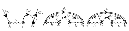
Figure 11: To study the renormalization of RKKY and usual Kondo couplings, we can extend the Poorman diagrams to include RKKY vertices represented by crossed circles and the usual J vertices with black circles. Three spin-flip processes are absent in the single impurity case at the second-order process. To distinguish between different types of interactions, we can use a wavy line to denote RKKY interactions and a dotted line to denote impurity-$mathcal{DM}$ interactions.

The above discussion highlights the difficulty in computing all diagrams at third order in the presence of both RKKY and $\mathcal{DM}$ interactions. With ${}^{7}C_{2}$ diagrams possible at second order and ${}^{7}C_{2}+{}^{7}C_{3}$ diagrams possible at third order, the calculations become extremely tedious. However, one can use algebraic techniques to simplify the computation in scenarios with potential scattering. Lie matrices can be used to compute the contributions in such cases.

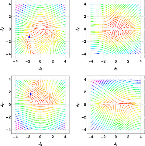
Figure 12: The above panels in the first row correspond to the positive root and $m=-4$ and in the real, imaginary plane, similarly below for the negative root and $m=-4$, showing the spiral FP in RG flow.

Appendix D RKKY Interaction

We can write the RKKY interaction in edge states by expanding in the Fourier series for the spins,

$$\begin{split}J_{Y}(r_{i}-r_{j})&\propto\sum_{kk^{\prime}hh^{\prime}}\frac{V_{ij}}{\epsilon_{kh}-\epsilon_{k^{\prime}h^{\prime}}}e^{ik(r_{i}-r_{j})}V^{*}_{ij}e^{-ik^{\prime}(r_{i}-r_{j})}\\ &=\int^{2\pi}_{0}\int^{\pi}_{0}\int^{k_{f}}_{0}\frac{k^{2}sin\theta e^{ikR}dkd\theta d\phi}{\sqrt{k^{6}\beta^{2}\cos^{2}3\theta+k^{2}}}+(k\neq k^{\prime},h=h^{\prime})\hskip 5.69054pt\text{terms}\end{split}$$ (36)

We solve the above integral the same way as we evaluate in impurity transport sections and show that the leading contribution for $J_{Y}$ is the sum of special functions as $E_{1}(\epsilon)+E_{2}(\epsilon)$ with substitution $\cos\theta=t$ we get following also we don’t set $\epsilon_{k}=\epsilon_{k^{\prime}}$ as in the Poorman limit instead we consider a chemical potential such that integral does not diverge in this limit,

$$\begin{split}J_{Y}&\propto\pi\int_{k}\frac{e^{ikR}}{k\beta}\oint\frac{qdt}{q^{2}-(4t^{3}-3t)^{2}}+\sum_{kk^{\prime}}\frac{|V_{ij}|}{k^{2}-(k^{\prime})^{2}}e^{ikr}e^{-ik^{\prime}r}\\ &\text{where}\hskip 5.69054ptq=\frac{\sqrt{(k^{2}-\epsilon)^{2}-k^{2}}}{\beta k^{3}}\\ \therefore J_{Y}&\propto\int e^{i\sqrt{\epsilon}r}\frac{\sqrt{(\epsilon-\epsilon^{\prime})^{2}-\epsilon}}{\beta\epsilon^{\frac{3}{2}}}\sqrt{\epsilon}d\epsilon+\frac{\sin(\sqrt{\epsilon}r)}{\epsilon^{\frac{3}{2}}}+\frac{\sin(\sqrt{\epsilon}r)}{\sqrt{\epsilon}}..\end{split}$$ (37)

We can immediately see the sum of the roots will vanish for such cubic equations since there is no $t^{2}$ coefficient, but the quantity in the root is not the same for all residues; hence it does contribute. Here we show the first part of the integral has a root structure and can be scaled with the root and can be identified why there is critical $\epsilon^{\prime}=-0.25$ for rkky although there are even and odd terms in series. The second term is standard considered in various studies shown explicitly in pointlike contact potential, it can be expressed as bessel function[63] or elliptic function[64](can be expressed in both special functions).

$$\begin{split}J_{Y}&\propto\sum^{\infty}_{n=0}i^{n}\frac{2\sqrt{\epsilon^{\prime 2}-2\epsilon^{\prime}\epsilon+(\epsilon-1)\epsilon}r^{n}\epsilon^{n/2}F_{1}\left(\frac{n}{2};-\frac{1}{2},-\frac{1}{2};\frac{n}{2}+1;-\frac{2\epsilon}{-2\epsilon^{\prime}+\sqrt{4\epsilon^{\prime}+1}-1},\frac{2\epsilon}{2\epsilon^{\prime}+\sqrt{4\epsilon^{\prime}+1}+1}\right)}{nn!\sqrt{\frac{2\epsilon^{\prime}+\sqrt{4\epsilon^{\prime}+1}-2\epsilon+1}{2\epsilon^{\prime}+\sqrt{4\epsilon^{\prime}+1}+1}}\sqrt{\frac{-2\epsilon^{\prime}+\sqrt{4\epsilon^{\prime}+1}+2\epsilon-1}{-2\epsilon^{\prime}+\sqrt{4\epsilon^{\prime}+1}-1}}}+\frac{\sin(\sqrt{\epsilon}r)}{\epsilon^{\frac{3}{2}}}+\frac{\sin(\sqrt{\epsilon}r)}{\sqrt{\epsilon}}..\end{split}$$ (38)

The first term is a sum and can be shown as an odd and even $J_{Y}=\sum^{\infty}_{n=0}=J^{odd}_{Y}+J^{even}_{Y}$ so therefore, all the odd terms can be expressed as the elliptic functions graphically shown in the main article in figure 10 which host exceptional points. Even terms consist of transcendental functions

Appendix E Analytic Solution of RG equations

A natural simplification of $J_{k^{3}}$ and $J_{k}$ RG equation by eliminating $J_{0}$ gives the following,

$$\begin{split}\frac{dJ_{k^{3}}}{dl}-J^{2}_{k}=\frac{J_{k^{3}}}{J_{k}}\frac{dJ_{k}}{dl}\\ \frac{1}{J_{k^{3}}}\frac{dJ_{k^{3}}}{dl}-\frac{J^{2}_{k}}{J_{k^{3}}}=\frac{1}{J_{k}}\frac{dJ_{k}}{dl}\end{split}$$ (39)

Now with a substitution of $\frac{J^{2}_{k}}{J_{k^{3}}}=x$ which gives upon differentiation $\frac{dx}{dl}=2\frac{J_{k}}{J_{k^{3}}}\frac{dJ_{k}}{dl}-\frac{J^{2}_{k}}{J^{2}_{k^{3}}}\frac{dJ_{k^{3}}}{dl}$ using this and rearranging we get solution as $J_{k}=-\frac{1}{2}\pm\frac{1}{2}\sqrt{1+4mJ_{k^{3}}}$ this is related to second solution by phase factors Now we can derive the full solution as the following,

$$\begin{split}J_{0}\frac{dJ_{0}}{dl}-J^{3}_{0}=n,\hskip 5.69054pt\bigg{(}\frac{J^{2}_{k}+J_{k}}{m}+J_{k}\frac{(J_{k}+1)^{2}}{m^{2}}+J_{k}\bigg{)}\frac{dJ_{k}}{dl}=n\end{split}$$ (40)

This yield solution is as follows; One can show the m has complex roots when the effective bandwidth vanishes. $J^{*}_{k}\to\frac{\sqrt{3}e^{i\frac{\pi}{3}}}{2}$,$J^{*}_{k^{3}}\to\frac{9e^{i\frac{\pi}{3}}}{16}$ and $m=e^{i\frac{\pi}{3}}$ where the $J^{*}_{0}$ will have $\tan^{-1}(..)$ quantity vanishing for $J^{*}_{0}=\pm 1$ in ferromagnetic and antiferromagnetic cases for $n\to 1$ see equations in 41, also log contribution to scale vanish when $J^{*}_{0}=-2$.We get these FP’s when we add the potential scattering terms.

$$\begin{split}\log\bigg{(}\frac{[m^{2}+m(J_{k}-1)+(J_{k}-1)^{2}]^{3\gamma}}{J^{2\gamma}_{k}}\bigg{)}+\frac{(m-2)}{\sqrt{3}(m^{2}-m+1)}\tan^{-1}\left(\frac{m+2J_{k}-2}{\sqrt{3}m}\right)=n\log D_{eff}\\ \frac{\log\left(n^{2/3}+\sqrt[3]{n}(-J_{0})+J_{0}^{2}\right)-2\log\left(\sqrt[3]{n}+J_{0}\right)-2\sqrt{3}\tan^{-1}\left(\frac{1-\frac{2J_{0}}{\sqrt[3]{n}}}{\sqrt{3}}\right)}{6\sqrt[3]{n}}=\log D_{eff}\\ \text{where}\hskip 5.69054pt\gamma=\frac{-m}{6*(m^{2}-m+1)}\implies\gamma\to-\infty*\hskip 5.69054pt\text{for}\hskip 5.69054ptm=e^{\pm i\frac{\pi}{3}}\end{split}$$ (41)

Due to the bath’s exceptional dispersion, there may be an unusual impurity screening. The kondo destruction will be at the critical points found above, leading to some complex FPs. The similarity between the RG of a single impurity in edge states and two impurities in conventional Fermi gas. For this reason, we solve two-impurity problem RG equations by limiting all couplings to zero except $J_{0}\neq J_{Y}\neq K\neq 0$.We need to solve the equations $\frac{dJ_{0}}{dl}=J^{2}_{0}+J_{Y}J_{0}+KJ_{0},\frac{dJ_{Y}}{dl}=J^{2}_{Y}+J^{2}_{0}+K^{2},\frac{dK}{dl}=K^{2}+KJ_{Y}$. If we solve $J_{0}$ and K equations, we get $J_{0}=\frac{RK}{K-1}$ as a solution where R is a constant or invariant under renormalization. Using this solution, we solve $J_{Y}$ and K equations as follows,

$$\begin{split}J_{Y}\frac{dJ_{Y}}{dl}-J^{3}_{Y}=R_{1},\frac{dK}{dl}-K^{2}=\frac{R_{1}}{\frac{R^{2}K}{(1-K)^{2}}+K}\\ \frac{-2\log\left(J_{Y}+\sqrt[3]{R_{1}}\right)+\log\left(\sqrt[3]{R_{1}}\left(-J_{Y}\right)+J_{Y}^{2}+R_{1}^{2/3}\right)+2\sqrt{3}\tan^{-1}\left(\frac{\frac{2J_{Y}}{\sqrt[3]{R_{1}}}-1}{\sqrt{3}}\right)}{6\sqrt[3]{R_{1}}}=\log D_{eff}\\ \frac{-2\log\left(K+\sqrt[3]{R_{1}}\right)+\log\left(\sqrt[3]{R_{1}}\left(-K\right)+K^{2}+R_{1}^{2/3}\right)+2\sqrt{3}\tan^{-1}\left(\frac{\frac{2K}{\sqrt[3]{R_{1}}}-1}{\sqrt{3}}\right)}{6\sqrt[3]{R_{1}}}=\log D_{eff},\hskip 5.69054pt\text{for}\hskip 5.69054ptK\to\infty\\ \frac{-\frac{R^{2}}{K-1}+R^{2}\log(K-1)+\frac{1}{2}(K-1)^{2}+K}{R_{1}}=\log D_{eff},\hskip 5.69054pt\text{for}\hskip 5.69054ptK\to 0\\ (K-1)^{\frac{R}{R_{1}}}\exp{\frac{1}{R_{1}}\bigg{(}-\frac{R^{2}}{K-1}+\frac{1}{2}(K-1)^{2}+K\bigg{)}}=D_{eff}\\ \implies(KR/J_{0})^{\frac{R}{R_{1}}}e^{\frac{1}{R_{1}}\bigg{(}-\frac{R^{2}}{KR/J_{0}}+\frac{1}{2}(KR/J_{0})^{2}+K\bigg{)}}=D_{eff}\\ \frac{\sqrt[3]{R_{1}}\left(-J_{Y}\right)+J_{Y}^{2}+R_{1}^{2/3}}{(J_{Y}+\sqrt[3]{R_{1}})^{2}}e^{2\sqrt{3}\tan^{-1}\left(\frac{\frac{2J_{Y}}{\sqrt[3]{R_{1}}}-1}{\sqrt{3}}\right)}=D^{6R^{\frac{1}{3}}_{1}}_{eff}\end{split}$$ (42)

Solving for $D_{eff}$ we can see how the two impurity kondo scale renormalized in this problem. Similarly, We will solve the $J_{0}$ equation with $J_{Y}$ to separate the solutions and for $R=R_{1}=1.0$, we show the flow and critical points. We expect FP’s in different quadrants depending on the sign we choose for these constants.

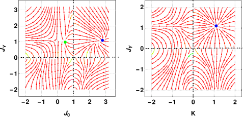
Figure 13: Plots above show the FP can be in different quadrants with $R_{1}=-1$ and $R=1.0$. We get around the spiral FP’s we get sign reversion in couplings.

Appendix F Impurity Transport Calculation

We follow the $\mathcal{T}_{kk^{\prime}}$ formalism (without expanding in terms of $\Delta$ as we did for separating RG flow and also not including the potential scatterings) for the derived kondo model after the k-dependent unitary to compute the relaxation time as follows,

$$\begin{split}\frac{1}{\tau(k)}\propto(1-2J\tilde{g}_{\alpha}(\epsilon_{k})-2J\tilde{g}_{\alpha}^{*}(\epsilon_{k})-2J_{k^{3}}\tilde{g}_{\alpha k^{3}}(\epsilon_{k})-2J_{k^{3}}\tilde{g}_{\alpha k^{3}}^{*}(\epsilon_{k})-2J_{k}\tilde{g}_{\alpha k}(\epsilon_{k})-2J_{k}\tilde{g}_{\alpha k}^{*}(\epsilon_{k}))\end{split}$$ (43)

$$\begin{split}\tilde{g}_{\alpha}(\epsilon)=\int^{2\pi}_{0}\int^{\pi}_{0}\int^{k_{f}}_{0}\frac{k^{2}sin\theta dkd\theta d\phi}{k^{2}+\alpha\sqrt{k^{6}\beta^{2}\cos^{2}3\theta+k^{2}}-\epsilon}\end{split}$$ (44)

Solving the $\theta$ integral first, we get two pieces as follows,

$$\begin{split}\tilde{g}_{\alpha}(\epsilon)=2\pi\int_{k}k^{2}\oint\frac{dt}{k^{2}+\alpha\sqrt{k^{6}\beta^{2}(4t^{3}-3t)^{2}+k^{2}}-\epsilon}\end{split}$$ (45)

we rationalize the above integral and write as the following by introducing $q=\frac{\sqrt{(k^{2}-\epsilon)^{2}-k^{2}}}{\beta k^{3}}$,

$$\begin{split}\tilde{g}_{\alpha}(\epsilon)&=2\pi\int_{k}\frac{1}{k}\oint\frac{q+\bar{\alpha}\sqrt{(4t^{3}-3t)^{2}+\frac{1}{\beta^{2}k^{4}}}dt}{q^{2}-(4t^{3}-3t)^{2}}\\ &=\pi\int_{k}\frac{1}{kq}\oint\frac{q+\bar{\alpha}\sqrt{(4t^{3}-3t)^{2}+\frac{1}{\beta^{2}k^{4}}}dt}{q-(4t^{3}-3t)}+\pi\int_{k}\frac{1}{kq}\oint\frac{q+\bar{\alpha}\sqrt{(4t^{3}-3t)^{2}+\frac{1}{\beta^{2}k^{4}}}dt}{q+(4t^{3}-3t)}\\ &=\int_{k}\frac{\pi}{kq}\bigg{(}\sum_{res}f(t,q)+\sum_{res}f(t,-q)\bigg{)}\end{split}$$ (46)

For finding these residues, we will use the roots of the cubic equations $\beta(4t^{3}-3t)\pm q=0$. We collect positive q roots and negative as follows for doing contour integrals,

$$\begin{split}t^{+}=\begin{cases}\frac{1}{2}\left(\sqrt[3]{\sqrt{q^{2}-1}+q}+\frac{1}{\sqrt[3]{\sqrt{q^{2}-1}+q}}\right),\\ -\frac{1}{4}\left(1-i\sqrt{3}\right)\sqrt[3]{\sqrt{q^{2}-1}+q}-\frac{1+i\sqrt{3}}{4\sqrt[3]{\sqrt{q^{2}-1}+q}}\\ -\frac{1}{4}\left(1+i\sqrt{3}\right)\sqrt[3]{\sqrt{q^{2}-1}+q}-\frac{1-i\sqrt{3}}{4\sqrt[3]{\sqrt{q^{2}-1}+q}}\end{cases}t^{-}=\begin{cases}\frac{1}{2}\left(\sqrt[3]{\sqrt{q^{2}-1}-q}+\frac{1}{\sqrt[3]{\sqrt{q^{2}-1}-q}}\right),\\ -\frac{1}{4}\left(1-i\sqrt{3}\right)\sqrt[3]{\sqrt{q^{2}-1}-q}-\frac{1+i\sqrt{3}}{4\sqrt[3]{\sqrt{q^{2}-1}-q}}\\ -\frac{1}{4}\left(1+i\sqrt{3}\right)\sqrt[3]{\sqrt{q^{2}-1}-q}-\frac{1-i\sqrt{3}}{4\sqrt[3]{\sqrt{q^{2}-1}-q}}\end{cases}\end{split}$$ (47)

Similarly, the other contributions are as follows,

$$\begin{split}\tilde{g}_{\alpha k^{3}}(\epsilon)&=2\pi\beta\int_{k}k^{2}\oint\frac{((4t^{3}-3t)^{2})(q+\bar{\alpha}\sqrt{(4t^{3}-3t)^{2}+\frac{1}{\beta^{2}k^{4}}})}{q^{2}-(4t^{3}-3t)^{2}}dt\\ \tilde{g}_{\alpha k}(\epsilon)&=\int_{k}\oint\frac{(q+\bar{\alpha}\sqrt{(4t^{3}-3t)^{2}+\frac{1}{\beta^{2}k^{4}}})}{q^{2}-(4t^{3}-3t)^{2}}dt\end{split}$$ (48)

after summing over the $\alpha=\pm$ bands we get following simplifications,

$$\begin{split}\tilde{g}_{\alpha}(\epsilon)&=2\pi\int_{k}\frac{1}{k}\oint\frac{qdt}{q^{2}-(4t^{3}-3t)^{2}},\tilde{g}_{\alpha k^{3}}(\epsilon)=2\pi\beta\int_{k}k^{2}\oint\frac{(4t^{3}-3t)^{2}qdt}{q^{2}-(4t^{3}-3t)^{2}},\tilde{g}_{\alpha k}(\epsilon)=\int_{k}\oint\frac{qdt}{q^{2}-(4t^{3}-3t)^{2}}\end{split}$$ (49)

After contour integrals we can show each integral contributes as $\oint\frac{dt}{q^{2}-(4t^{3}-3t)^{2}}=q$ hence sum of all $(g_{\alpha})$ contribution as following,

$$\begin{split}\tilde{g}_{\epsilon}=\int(\beta qk^{2}-\beta q^{4}k+\frac{q}{k}-q)dk\end{split}$$ (50)

We know from derivation $\epsilon\approx k^{2}$ and the density of states in 3D as $\rho(\epsilon)\approx\sqrt{\epsilon}$ then above integral yields,

$$\begin{split}\tilde{g}_{\epsilon^{\prime}}=\int\bigg{(}\frac{\sqrt{(\epsilon-\epsilon^{\prime})^{2}-\epsilon}}{\sqrt{\epsilon}}-\frac{((\epsilon-\epsilon^{\prime})^{2}-\epsilon)^{2}}{\beta^{3}\epsilon^{6-\frac{1}{2}}}+\frac{\sqrt{(\epsilon-\epsilon^{\prime})^{2}-\epsilon}}{\beta\epsilon^{2}}-\frac{\sqrt{(\epsilon-\epsilon^{\prime})^{2}-\epsilon}}{\beta\epsilon^{\frac{3}{2}}}\bigg{)}d\epsilon\end{split}$$ (51)

Where in above $\epsilon^{\prime}$ is the chemical potential can take any values around fermi energy. We perform this above integral exactly in terms of special functions to extract contribution to $\frac{1}{\tau}$, which indeed scales with RG invariant in the elliptic functions.

$$\begin{split}&\tilde{g}_{\epsilon}\propto\frac{P_{1}(\epsilon)+P_{\frac{3}{2}}(\epsilon)+T_{1}(\epsilon)+E_{1}(\epsilon)+E_{2}(\epsilon)+\log(\epsilon)}{\beta^{3}}\\ &P_{1}(\epsilon)=-\frac{3\epsilon^{\prime 4}-16\epsilon^{\prime 3}\epsilon+4\epsilon^{\prime 2}\epsilon(9\epsilon-2)+2\epsilon^{2}\left(2\epsilon\left(\beta^{2}\sqrt{(\epsilon^{\prime}-\epsilon)^{2}-\epsilon}\left(2\sqrt{\epsilon}(\beta-\beta\epsilon+3)+3\right)-6\right)+3\right)}{12\epsilon^{4}}\\ &P_{\frac{3}{2}}(\epsilon)=\frac{8\epsilon^{\prime}\epsilon^{2}\left(2\beta^{3}\epsilon^{3/2}\sqrt{(\epsilon^{\prime}-\epsilon)^{2}-\epsilon}-6\epsilon+3\right)}{12\epsilon^{4}}\\ &T_{1}(\epsilon)=\beta^{2}\tanh^{-1}\left(\frac{-2\epsilon^{\prime}+2\epsilon-1}{2\sqrt{(\epsilon^{\prime}-\epsilon)^{2}-\epsilon}}\right)+\frac{(2\epsilon^{\prime}+1)\beta^{2}\coth^{-1}\left(\frac{2\epsilon^{\prime}\sqrt{(\epsilon^{\prime}-\epsilon)^{2}-\epsilon}}{2\epsilon^{\prime}(\epsilon^{\prime}-\epsilon)-\epsilon}\right)}{2\epsilon^{\prime}}\\ &E_{1}(\epsilon)=\frac{i\beta^{2}\epsilon\sqrt{\frac{-2\epsilon^{\prime}+\sqrt{4\epsilon^{\prime}+1}+2\epsilon-1}{\epsilon}}\sqrt{-\frac{2\epsilon^{\prime}+\sqrt{4\epsilon^{\prime}+1}-2\epsilon+1}{\epsilon}}\left(AE\left(i\sinh^{-1}\left(\frac{\sqrt{-2\epsilon^{\prime}-\sqrt{4\epsilon^{\prime}+1}-1}}{\sqrt{2}\sqrt{\epsilon}}\right)|\frac{2\epsilon^{\prime}-\sqrt{4\epsilon^{\prime}+1}+1}{2\epsilon^{\prime}+\sqrt{4\epsilon^{\prime}+1}+1}\right)\right)}{3\sqrt{2}\sqrt{-2\epsilon^{\prime}-\sqrt{4\epsilon^{\prime}+1}-1}\sqrt{(\epsilon^{\prime}-\epsilon)^{2}-\epsilon}}\\ &A=\left(2\epsilon^{\prime}+\sqrt{4\epsilon^{\prime}+1}+1\right)(2\epsilon^{\prime}\beta+\beta+6)\\ &E_{2}(\epsilon)=-\frac{B\left(\left(\sqrt{4\epsilon^{\prime}+1}+2\epsilon^{\prime}\left(\sqrt{4\epsilon^{\prime}+1}+2\right)+1\right)\beta+6\sqrt{4\epsilon^{\prime}+1}\right)F\left(i\sinh^{-1}\left(\frac{\sqrt{-2\epsilon^{\prime}-\sqrt{4\epsilon^{\prime}+1}-1}}{\sqrt{2}\sqrt{\epsilon}}\right)|\frac{2\epsilon^{\prime}-\sqrt{4\epsilon^{\prime}+1}+1}{2\epsilon^{\prime}+\sqrt{4\epsilon^{\prime}+1}+1}\right)}{3\sqrt{2}\sqrt{-2\epsilon^{\prime}-\sqrt{4\epsilon^{\prime}+1}-1}\sqrt{(\epsilon^{\prime}-\epsilon)^{2}-\epsilon}}\\ &B=i\beta^{2}\epsilon\sqrt{\frac{-2\epsilon^{\prime}+\sqrt{4\epsilon^{\prime}+1}+2\epsilon-1}{\epsilon}}\sqrt{-\frac{2\epsilon^{\prime}+\sqrt{4\epsilon^{\prime}+1}-2\epsilon+1}{\epsilon}}\end{split}$$ (52)

In the above solution, F is an incomplete elliptic function of the first kind, and E is an elliptic function of the second kind. P and T are polynomial and transcendental functions, respectively.Similar elliptic functions are found to solve nonhermitian problem [34] to connect the nonequilibrium self-energy of an open system.

Appendix G Numerical Solutions

G.1 Solutions for RG ODE’s

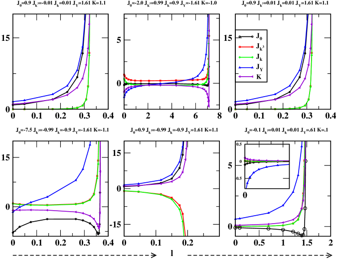
Figure 14: We plot the solutions of the RG equations around the critical points from the flow diagram. The x-axis is the bandwidth diverging points corresponding to the Kondo scale, and cusp-like behaviors indicate the two impurity model FP’s. The inset graph shows the non-interacting FP we got when we set either $J_{Y}$ or $K$ to negative otherwise, we have two impurities Kondo effect, where all couplings diverge. SR in both can be seen for the couplings $J_{0},K$ when for both $J_{k^{3}},J_{k}$ given -ve initial conditions(IC) are given. Otherwise, only the $K$ reverses sign with cusp $-\infty\to\infty$.With various IC’s, we verified it is necessary to have $J_{k^{3}}\neq 0$ to get cusp-like sign reversion in the couplings. IC’s are mentioned above each plot above.

G.2 Single Impurity Case

The solutions are examined for the spiral FP’s whether we have SR in the imaginary part of the RG beta functions $\beta_{n}$. Indeed we verify FP’s corresponding to two spiral points and one marginal point, all of them a reverse sign, whereas we had negative $\beta_{n}$ when all the couplings are very small except $J_{0}$ shown in figure 15. From the invariant derived analytically $J_{k}=\frac{1}{2}\pm\frac{1}{2}\sqrt{1+4mJ_{k^{3}}}$ for $J_{k^{3}}=0.5$(that is where we got FP see fig 5 of main paper) and $m=4$ we get two roots as $J_{k}=\frac{1}{2}\pm\frac{3}{2}=2,-1$ exactly these were chosen as initial conditions and shown $\beta_{n}\to\beta^{*}_{n}$.We also have various 3-pole and 2-pole regimes where we don’t have FP’s.

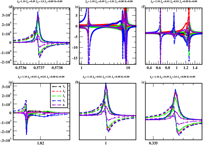
Figure 15: We plot the solutions of the RG equations around the critical points from the flow diagram for the single impurity case($K=J_{Y}=0$). plots (c) and (d) correspond to spiral FP’s and plot (b) is marginal point case when $J_{k^{3}}=0,J_{k}=\frac{1}{2}\pm\frac{1}{2}\sqrt{1+4mJ_{k^{3}}}=0,1$. plot (a) is usual Kondo when homogeneous bath case so that all set zero except $J_{0}\neq 0$.Plots (e) and (f) are the solutions where flow is divergent with no FP.

G.3 Two Impurity Case

Unlike single impurity cases, we do not have the flow FP’s in the TIK problem; hence we need to generate many data files to identify where the SR regime exists. We can set $J_{k^{3}}=J_{k}=0$ and start analyzing, and we find the SR regime for the spiral points. But in general, this is a rich problem and requires more analysis, but here we show a critical $J_{k^{3}}$ required to get SR in figure 14. Having the SR scenarios in RG indicate there is the emergence of complex solutions as found by analytically and numerically in a single impurity.

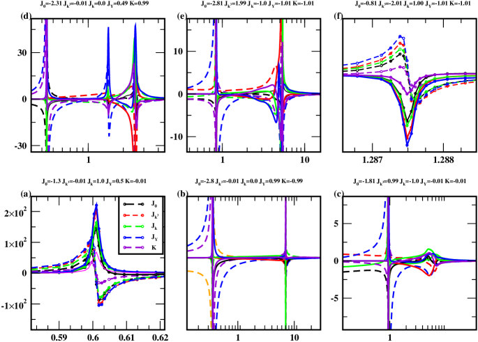
Figure 16: We plot the RG solutions by allowing the complex solutions of RG nonlinear equations. The dotted and thick lines correspond to real and imaginary coupling values. Sign reversion in all couplings is captured when we have a critical value of the nonlinear coupling $J_{k^{3}}>2.0$. Between the two sign-reversing phases in plots $a\to f$, there are various 2-pole(b,c,e) and 3-pole(d) regimes. This confirms the spiral FP’s we got are due to the sign reversion in couplings. This happens only at two initial conditions. Scales above the $10^{3}$ are not labeled in y - the axis and all plots’ x-axis is a flow parameter which is either in log/linear scale.The sign-reversing phase happens in imaginary values of couplings equivalently RG beta functions $\beta_{n}\to\beta_{n}^{*}$ also mean a renormalized self-energy $\tilde{\Sigma}(l)\to\tilde{\Sigma}(l)^{*}$ which is equivalent of getting EP in odd coupling in this problem. The central idea of this analysis is that there is an exceptional point in $J^{odd}_{Y}$ and in bath integrals $E_{1}+E_{2}$ to verify if at all there exist $J_{k^{3}}$ values for which this transition occurs. There are $10^{5}$ data files for 10 IC’s hence it requires further analysis to find other values at which this happens.

References

- Lü et al. [2013] H.-F. Lü, H.-Z. Lu, S.-Q. Shen, and T.-K. Ng, Quantum impurity in the bulk of a topological insulator, Phys. Rev. B 87, 195122 (2013).
- Mitchell et al. [2013] A. K. Mitchell, D. Schuricht, M. Vojta, and L. Fritz, Kondo effect on the surface of three-dimensional topological insulators: Signatures in scanning tunneling spectroscopy, Phys. Rev. B 87, 075430 (2013).
- Dey et al. [2018] U. Dey, M. Chakraborty, A. Taraphder, and S. Tewari, Bulk band inversion and surface dirac cones in lasb and labi: Prediction of a new topological heterostructure, Scientific Reports 8, 14867 (2018).
- Li et al. [2009] J. Li, R.-L. Chu, J. K. Jain, and S.-Q. Shen, Topological anderson insulator, Phys. Rev. Lett. 102, 136806 (2009).
- Kuzmenko et al. [2014] I. Kuzmenko, Y. Avishai, and T. K. Ng, Anderson impurity in the bulk of topological insulators, Phys. Rev. B 89, 035125 (2014).
- Boettcher [2020] I. Boettcher, Interplay of topology and electron-electron interactions in rarita-schwinger-weyl semimetals, Phys. Rev. Lett. 124, 127602 (2020).
- Sierra et al. [2018] M. A. Sierra, R. López, and J. S. Lim, Thermally driven out-of-equilibrium two-impurity kondo system, Phys. Rev. Lett. 121, 096801 (2018).
- Affleck and Ludwig [1992] I. Affleck and A. W. Ludwig, Exact critical theory of the two-impurity kondo model, Physical review letters 68, 1046 (1992).
- Mitchell et al. [2012] A. K. Mitchell, E. Sela, and D. E. Logan, Two-channel kondo physics in two-impurity kondo models, Physical review letters 108, 086405 (2012).
- Silva et al. [1996] J. Silva, W. Lima, W. Oliveira, J. Mello, L. N. d. Oliveira, and J. Wilkins, Particle-hole asymmetry in the two-impurity kondo model, Physical review letters 76, 275 (1996).
- O’Bannon et al. [2016] A. O’Bannon, I. Papadimitriou, and J. Probst, A holographic two-impurity kondo model, Journal of High Energy Physics 2016, 1 (2016).
- Sela et al. [2011] E. Sela, A. K. Mitchell, and L. Fritz, Exact crossover green function in the two-channel and two-impurity kondo models, Physical review letters 106, 147202 (2011).
- Gan [1995a] J. Gan, Solution of the two-impurity kondo model: Critical point, fermi-liquid phase, and crossover, Physical Review B 51, 8287 (1995a).
- Gan [1995b] J. Gan, Mapping the critical point of the two-impurity kondo model to a two-channel problem, Physical review letters 74, 2583 (1995b).
- Bayat et al. [2012] A. Bayat, S. Bose, P. Sodano, and H. Johannesson, Entanglement probe of two-impurity kondo physics in a spin chain, Physical Review Letters 109, 066403 (2012).
- Mross and Johannesson [2009a] D. F. Mross and H. Johannesson, Two-impurity kondo model with spin-orbit interactions, Physical Review B 80, 155302 (2009a).
- Cho and McKenzie [2006] S. Y. Cho and R. H. McKenzie, Quantum entanglement in the two-impurity kondo model, Physical Review A 73, 012109 (2006).
- Sire et al. [1993] C. Sire, C. M. Varma, and H. Krishnamurthy, Theory of the non-fermi-liquid transition point in the two-impurity kondo model, Physical Review B 48, 13833 (1993).
- Campo Jr and Oliveira [2004] V. L. Campo Jr and L. N. Oliveira, Thermodynamics for the two-impurity kondo model, Physical Review B 70, 153401 (2004).
- Hallberg and Egger [1997] K. Hallberg and R. Egger, Two-impurity kondo problem for correlated electrons, Physical Review B 55, R8646 (1997).
- Principi et al. [2015] A. Principi, G. Vignale, and E. Rossi, Kondo effect and non-fermi-liquid behavior in dirac and weyl semimetals, Phys. Rev. B 92, 041107 (2015).
- Liu et al. [2010] C.-X. Liu, X.-L. Qi, H. Zhang, X. Dai, Z. Fang, and S.-C. Zhang, Model hamiltonian for topological insulators, Phys. Rev. B 82, 045122 (2010).
- Zhang et al. [2009] H. Zhang, C.-X. Liu, X.-L. Qi, X. Dai, Z. Fang, and S.-C. Zhang, Topological insulators in bi2se3, bi2te3 and sb2te3 with a single dirac cone on the surface, Nature physics 5, 438 (2009).
- Lü et al. [2019] H.-F. Lü, Y.-H. Deng, S.-S. Ke, Y. Guo, and H.-W. Zhang, Quantum impurity in topological multi-weyl semimetals, Phys. Rev. B 99, 115109 (2019).
- Mitchell and Fritz [2016] A. K. Mitchell and L. Fritz, Signatures of weyl semimetals in quasiparticle interference, Phys. Rev. B 93, 035137 (2016).
- Zarea et al. [2012] M. Zarea, S. E. Ulloa, and N. Sandler, Enhancement of the kondo effect through rashba spin-orbit interactions, Phys. Rev. Lett. 108, 046601 (2012).
- Mastrogiuseppe et al. [2014] D. Mastrogiuseppe, A. Wong, K. Ingersent, S. E. Ulloa, and N. Sandler, Kondo effect in graphene with rashba spin-orbit coupling, Phys. Rev. B 90, 035426 (2014).
- Zarea and Sandler [2009] M. Zarea and N. Sandler, Rashba spin-orbit interaction in graphene and zigzag nanoribbons, Phys. Rev. B 79, 165442 (2009).
- Žitko [2010] R. Žitko, Quantum impurity on the surface of a topological insulator, Phys. Rev. B 81, 241414 (2010).
- Lourenço et al. [2018] J. A. S. Lourenço, R. L. Eneias, and R. G. Pereira, Kondo effect in a -symmetric non-hermitian hamiltonian, Phys. Rev. B 98, 085126 (2018).
- Nakagawa et al. [2018] M. Nakagawa, N. Kawakami, and M. Ueda, Non-hermitian kondo effect in ultracold alkaline-earth atoms, Phys. Rev. Lett. 121, 203001 (2018).
- Michishita and Peters [2020] Y. Michishita and R. Peters, Equivalence of effective non-hermitian hamiltonians in the context of open quantum systems and strongly correlated electron systems, Phys. Rev. Lett. 124, 196401 (2020).
- Oguri and Sakano [2013] A. Oguri and R. Sakano, Exact interacting green’s function for the anderson impurity at high bias voltages, Phys. Rev. B 88, 155424 (2013).
- Kulkarni [2022] V. M. Kulkarni, Derivation of -symmetric sine-gordon model and its relevance to non-equilibrium, arXiv preprint arXiv:2211.00333 (2022).
- Nagai et al. [2020] Y. Nagai, Y. Qi, H. Isobe, V. Kozii, and L. Fu, Dmft reveals the non-hermitian topology and fermi arcs in heavy-fermion systems, Phys. Rev. Lett. 125, 227204 (2020).
- Fring and Taira [2020] A. Fring and T. Taira, Complex bps solitons with real energies from duality, Journal of Physics A: Mathematical and Theoretical 53, 455701 (2020).
- Zhen et al. [2015] B. Zhen, C. W. Hsu, Y. Igarashi, L. Lu, I. Kaminer, A. Pick, S.-L. Chua, J. D. Joannopoulos, and M. Soljačić, Spawning rings of exceptional points out of dirac cones, Nature 525, 354 (2015).
- Betancourt et al. [2016] J. Betancourt, S. Li, X. Dang, J. Burton, E. Tsymbal, and J. Velev, Complex band structure of topological insulator bi2se3, Journal of Physics: Condensed Matter 28, 395501 (2016).
- Affleck and Ludwig [1993] I. Affleck and A. W. Ludwig, Exact conformal-field-theory results on the multichannel kondo effect: single-fermion green’s function, self-energy, and resistivity, Physical Review B 48, 7297 (1993).
- Kulkarni [2021] V. M. Kulkarni, Functional renormalization analysis of bose-einstien condensation through complex interaction in harmonic oscillator; can bendixson criteria be extended to complex time?, arXiv preprint arXiv:2112.03035 (2021).
- Han et al. [2023] S. Han, D. J. Schultz, and Y. B. Kim, Complex fixed points of the non-hermitian kondo model in a luttinger liquid, arXiv preprint arXiv:2302.07883 (2023).
- Nándori et al. [2004] I. Nándori, U. D. Jentschura, K. Sailer, and G. Soff, Renormalization-group analysis of the generalized sine-gordon model and of the coulomb gas for dimensions, Phys. Rev. D 69, 025004 (2004).
- Cheng and Liu [2009] W. W. Cheng and J.-M. Liu, Decoherence from spin environment: Role of the dzyaloshinsky-moriya interaction, Phys. Rev. A 79, 052320 (2009).
- Nagaosa and Tokura [2013] N. Nagaosa and Y. Tokura, Topological properties and dynamics of magnetic skyrmions, Nature nanotechnology 8, 899 (2013).
- Mross and Johannesson [2009b] D. F. Mross and H. Johannesson, Two-impurity kondo model with spin-orbit interactions, Phys. Rev. B 80, 155302 (2009b).
- Jones and Varma [1987] B. A. Jones and C. M. Varma, Study of two magnetic impurities in a fermi gas, Phys. Rev. Lett. 58, 843 (1987).
- Jones et al. [1988] B. A. Jones, C. M. Varma, and J. W. Wilkins, Low-temperature properties of the two-impurity kondo hamiltonian, Phys. Rev. Lett. 61, 125 (1988).
- Mitchell and Fritz [2015] A. K. Mitchell and L. Fritz, Kondo effect in three-dimensional dirac and weyl systems, Phys. Rev. B 92, 121109 (2015).
- Wójcik and Kroha [2023a] K. P. Wójcik and J. Kroha, Quantum spin liquid in an rkky-coupled two-impurity kondo system, Phys. Rev. B 107, L121111 (2023a).
- Wójcik and Kroha [2023b] K. P. Wójcik and J. Kroha, Asymmetry effects on the phases of rkky-coupled two-impurity kondo systems, Phys. Rev. B 107, 125146 (2023b).
- Hewson [1997] A. C. Hewson, The Kondo problem to heavy fermions, Vol. 2 (Cambridge university press, 1997).
- Yoshimura et al. [2020] T. Yoshimura, K. Bidzhiev, and H. Saleur, Non-hermitian quantum impurity systems in and out of equilibrium: Noninteracting case, Physical Review B 102, 125124 (2020).
- Kulkarni et al. [2022] V. M. Kulkarni, A. Gupta, and N. S. Vidhyadhiraja, Kondo effect in a non-hermitian -symmetric anderson model with rashba spin-orbit coupling, Phys. Rev. B 106, 075113 (2022).
- Zhang et al. [2021] W. Zhang, X. Ouyang, X. Huang, X. Wang, H. Zhang, Y. Yu, X. Chang, Y. Liu, D.-L. Deng, and L.-M. Duan, Observation of non-hermitian topology with nonunitary dynamics of solid-state spins, Phys. Rev. Lett. 127, 090501 (2021).
- Harari et al. [2018] G. Harari, M. A. Bandres, Y. Lumer, M. C. Rechtsman, Y. D. Chong, M. Khajavikhan, D. N. Christodoulides, and M. Segev, Topological insulator laser: theory, Science 359, eaar4003 (2018).
- Qin et al. [2023] F. Qin, R. Shen, and C. H. Lee, Non-hermitian squeezed polarons, Phys. Rev. A 107, L010202 (2023).
- Li et al. [2021] L. Li, C. H. Lee, and J. Gong, Impurity induced scale-free localization, Communications Physics 4, 42 (2021).
- Abrikosov [1965] A. A. Abrikosov, Electron scattering on magnetic impurities in metals and anomalous resistivity effects, Physics Physique Fizika 2, 5 (1965).
- Han et al. [2022] S. Han, D. J. Schultz, and Y. B. Kim, Non-fermi liquid behavior and quantum criticality in cubic heavy fermion systems with non-kramers multipolar local moments, Phys. Rev. B 106, 155155 (2022).
- Anderson [1970] P. Anderson, A poor man’s derivation of scaling laws for the kondo problem, Journal of Physics C: Solid State Physics 3, 2436 (1970).
- Sólyom [1974] J. Sólyom, Renormalization and scaling in the x-ray absorption and kondo problems, Journal of Physics F: Metal Physics 4, 2269 (1974).
- Sólyom and Zawadoswki [1974] J. Sólyom and A. Zawadoswki, Are the scaling laws for the kondo problem exact?, Journal of Physics F: Metal Physics 4, 80 (1974).
- Szałowski and Balcerzak [2008] K. Szałowski and T. Balcerzak, Rkky interaction with diffused contact potential, Phys. Rev. B 78, 024419 (2008).
- Okui [1974] S. Okui, Complete elliptic integrals resulting from integrals of bessel functions, Journal of Research of the National Bureau of Standards: Mathematical sciences. B , 113 (1974).