Dissipatons as generalized Brownian particles for open quantum systems: Dissipaton–embedded quantum master equation

Abstract

Dissipaton theory had been proposed as an exact and nonperturbative approach to deal with open quantum system dynamics, where the influence of Gaussian environment is characterized by statistical quasi-particles named as dissipatons. In this work, we revisit the dissipaton equation of motion theory and establish an equivalent dissipatons–embedded quantum master equation (DQME), which gives rise to dissipatons as generalized Brownian particles. As explained in this work, the DQME supplies a direct approach to investigate the statistical characteristics of dissipatons and thus the physically supporting hybrid bath modes. Numerical demonstrations are carried out on the electron transfer model, exhibiting the transient statistical properties of the solvation coordinate.

I Introduction

Open quantum systems are ubiquitous in various realms of physics.Wei21 ; Bre02 ; Yan05187 ; Lou73 ; Sli90 ; Van051037 ; Kli97 ; Ram98 ; Aka15056002 ; Muk81509 ; Yan885160 ; Yan91179 ; Che964565 ; Tan939496 ; Tan943049 ; Dor132746 ; Kun22015101 The system–environment interactions may lead to exchange of energy, particle and information between the open system and its surrounding environment. In literature, the environment is frequently known as baths or reservoirs. When the influence of surrounding environments (baths/reservoirs) cannot be neglected, quantum dissipation theories can be employed to describe the reduced system dynamics. Many quantum dissipation theories, such as the hierarchical equations of motion (HEOM) Tan89101 ; Tan906676 ; Tan06082001 ; Yan04216 ; Xu05041103 ; Xu07031107 ; Tan20020901 and the stochastic equation of motion (SEOM) Sha045053 ; Yan04216 ; Hsi18014104 ; Hsi18014104 theories, have been proposed, with focus mainly on the reduced system density operator, $\rho_{\mbox{\tiny S}}(t)\equiv{\rm tr}_{\mbox{\tiny B}}\rho_{\mbox{\tiny T}}(t)$.

However, it is well known that the reduced system dynamics alone, with relevant information encoded in $\rho_{\mbox{\tiny S}}(t)$, is insufficient to deal with all experimental measurements. The entangled system–and–environment dynamics are also crucially important in the study of strongly correlated quantum impurity systems. Imr02 ; Hau08 For example, the entangled system–environment correlation functions are closely related to such as spectroscopy, Zha15024112 ; Du20034102 ; Che21244105 transport Mei922512 ; Gru1624514 ; Wan20041102 ; Du212155 ; Wan22044102 and thermodynamics Kir35300 ; Gon20154111 ; Gon20214115 in quantum impurity systems. These properties are usually considered to be beyond the scope of traditional treatments by quantum dissipation theories. To address this issue, Yan proposed the dissipaton equation of motion (DEOM) in 2014, which provides a statistical quasi-particle picture for the influence of environment that can be either bosonic or fermionic. Yan14054105 ; Yan16110306 ; Wan22170901 The DEOM recovers fully the HEOM for the dynamics of the primarily reduced system density operator. Meanwhile, the underlying dissipaton algebra Yan14054105 ; Wan20041102 also makes the DEOM straightforward to study the hybrid bath dynamics, polarization and nonlinear coupling effects.Zha15024112 ; Xu151816 ; Wan22170901 ; Zha16204109 ; Yan16110306 ; Xu17395 ; Xu18114103 ; Su224554

The DEOM Yan14054105 is not only an “exact” (cf. comments at the end of Sec. II.1) and nonperturbative approach to the real–time evolution of open quantum system plus hybrid bath mode, but also serves as a prototype for the development of other equations of motion within the same framework of dissipaton theory but in different scenarios. For example, to study the Helmholtz free energy change due to the isotherm mixing of the system and environment, we proposed two independent approaches, the equilibrium $\lambda$-DEOM and imaginary–time DEOM.Gon20154111 Nonequilibrium $\lambda(t)$-DEOM is also recently developed to compute the nonequilibrium work distributions in system–environment mixing processes. Gon22054109 To exactly treat the nonlinear environment couplings, we propose to incorporate the stochastic fields, which resolve just the nonlinear environment coupling terms, into the DEOM construction. The resultant stochastic-fields-dressed (SFD) total Hamiltonian contains only linear environment coupling terms. On the basis of that, the SFD-DEOM was constructed. Che21174111 Besides, we also propose the dissipaton thermofield theory and obtain the system–bath entanglement theorem for nonequilibrium correlation functions.Wan22044102 All these theoretical ingredients comprise the family of dissipaton theories.

Remarkably, in above mentioned dissipaton theories, quasi-particle descriptions for baths can provide a unified treatment for the reduced system and hybridized environment dynamics. This is right the point of constructing an exact dissipaton theory, which is inspired by HEOM formalism and adopts dissipatons, etymologically derived from ther verb “dissipate” and the suffix “-on”, as quasi-particles associated with the Gaussian bath.Yan14054105 ; Yan16110306 ; Zha18780 ; Wan20041102 In this work, we revisit the dissipaton equation of motion theory and establish an equivalent dissipatons–embedded quantum master equation (DQME). In DQME, instead of a hierarchical structure, all the system–plus–dissipatons degrees of freedom are incorporated into a single dynamic equation. Specifically, we will demonstrate that dissipatons as generalized Brownian quasi-particles, whose distribution obeys a Smoluchowski dynamics. The DQME provides a direct approach to investigate the statistical characteristics of dissipatons and makes it convenient to obtain the hybrid bath modes dynamics. Therefore, the DQME itself thus serves as an important member of the family of dissipaton theories.

The remainder of this paper is organized as follows. In Sec. II, we briefly review the basic onsets of dissipaton theories. DQME is constructed in Sec. III. In Sec. IV, we detailedly discuss the statistical characteristics of dissipatons. The numerical demonstration is given in Sec. V, with the electron transfer model. We summarize this paper in Sec. VI. Throughout the paper we set $\hbar=1$ and $\beta=1/(k_{B}T)$, with $k_{B}$ the Boltzmann constant and $T$ the temperature.

II Onsets of dissipaton theory and DEOM

II.1 Prelude

Let us start from the basic system–plus–bath settings in the bosonic environment scenarios. For brevity, we only consider the single dissipative–mode cases, where the system–bath coupling assumes a linear form of $H_{\mbox{\tiny SB}}=\hat{Q}\hat{F}$. The total composite Hamiltonian tractable within the dissipaton theory has the generic form of

$$H_{\mbox{\tiny T}}=H_{\mbox{\tiny S}}+H_{\mbox{\tiny S}\mbox{\tiny B}}+h_{\mbox{\tiny B}}.$$ (1)

Both the system Hamiltonian $H_{\mbox{\tiny S}}$ and the dissipative system mode $\hat{Q}$ is arbitrary, whereas the hybrid reservoir bath mode $\hat{F}$ assumes to be linear. This together with noninteracting reservoir model of $h_{\mbox{\tiny B}}$ constitutes the Gauss–Wick’s environment ansatz, where the environmental influence is fully characterized by the hybridization bath reservoir correlation functions, $\langle\hat{F}_{\mbox{\tiny B}}(t)\hat{F}_{\mbox{\tiny B}}(0)\rangle_{\mbox{\tiny B}}$. Here, both $\hat{F}_{\mbox{\tiny B}}(t)\equiv e^{ih_{\mbox{\tiny B}}t}\hat{F}e^{-ih_{\mbox{\tiny B}}t}$ and the equilibrium canonical ensemble average, $\langle(\,\cdot\,)\rangle_{\mbox{\tiny B}}\equiv{\rm tr}_{\mbox{\tiny B}}[(\,\cdot\,)e^{-\beta h_{\mbox{\tiny B}}}]/{\rm tr}_{\mbox{\tiny B}}(e^{-\beta h_{\mbox{\tiny B}}})$ are defined in the bare–bath subspace. It can be related to the hybridize spectral density $J_{\mbox{\tiny B}}(\omega)$ via the fluctuation–dissipation theorem Wei21

$$\langle\hat{F}_{\mbox{\tiny B}}(t)\hat{F}_{\mbox{\tiny B}}(0)\rangle_{\mbox{\tiny B}}=\frac{1}{\pi}\!\int^{\infty}_{-\infty}\!\!{\rm d}\omega\,\frac{e^{-i\omega t}J_{\mbox{\tiny B}}(\omega)}{1-e^{-\beta\omega}}.$$ (2)

where

$$J_{\mbox{\tiny B}}(\omega)\equiv\frac{1}{2}\!\int^{\infty}_{-\infty}\!\!{\rm d}t\,e^{i\omega t}\langle[\hat{F}_{\mbox{\tiny B}}(t),\hat{F}_{\mbox{\tiny B}}(0)]\rangle_{\mbox{\tiny B}}.$$ (3)

The concept of dissipatons originates from an exponential series expansion of the hybridized bath correlation function, Yan16110306

$$\langle\hat{F}_{\mbox{\tiny B}}(t)\hat{F}_{\mbox{\tiny B}}(0)\rangle_{\mbox{\tiny B}}=\sum^{K}_{k=1}\eta_{k}e^{-\gamma_{k}t}.$$ (4a)

$$\langle\hat{F}_{\mbox{\tiny B}}(0)\hat{F}_{\mbox{\tiny B}}(t)\rangle_{\mbox{\tiny B}}=\sum^{K}_{k=1}\eta_{k}^{\ast}e^{-\gamma_{k}^{\ast}t}\equiv\sum^{K}_{k=1}\eta_{\bar{k}}^{\ast}e^{-\gamma_{k}t}.$$ (4b)

The exponential series expansion on $\langle\hat{F}_{\mbox{\tiny B}}(t)\hat{F}_{\mbox{\tiny B}}(0)\rangle_{\mbox{\tiny B}}$ can be achieved by adopting a certain sum–over–poles expression for the Fourier integrand on the right–hand–side of Eq.(2), followed by the Cauchy’s contour integration,Hu10101106 ; Hu11244106 ; Din11164107 ; Din12224103 ; Zhe121129 or using the time–domain Prony fitting decomposition scheme.Che22221102 Together with the time–reversal relation $\langle\hat{F}_{\mbox{\tiny B}}(0)\hat{F}_{\mbox{\tiny B}}(t)\rangle_{\mbox{\tiny B}}=\langle\hat{F}_{\mbox{\tiny B}}(t)\hat{F}_{\mbox{\tiny B}}(0)\rangle_{\mbox{\tiny B}}^{\ast}$ for $t\geq 0$. The second equality of Eq. (4b) is due to the fact that the exponents in Eq. (4a) must be either real or complex conjugate paired, and thus we may determine $\bar{k}$ in the index set $\{k=1,2,...,K\}$ by the pairwise equality $\gamma_{\bar{k}}=\gamma_{k}^{\ast}$.This is a crucial property. The exponential series expansion in Eqs. (4a) and (4b) inspired the idea of relating each exponential mode of correlation function to a statistical quasi-particle, i.e., a dissipaton.Yan14054105

It is worth noting that the decomposition in Eqs. (4a) and (4b) can be obtained via alternative methods including the Fano spectrum decomposition, Cui19024110 ; Zha20064107 the discrete Fourier series, Zho08034106 the extended orthogonal polynomials expansions, Liu14134106 ; Tan15224112 ; Nak18012109 ; Ike20204101 ; Lam193721 the time–domain Prony fitting scheme,Che22221102 and others. These methods have expanded the scope of application of HEOM/DEOM to the bath correlations in type of $\{t^{m}e^{-\gamma t}\}$ with $m$ a positive integer. The dissipaton theory can be extended to these scenarios and is numerically exact in these cases. However, the quest of the most general and exact decomposition scheme is still a challenge.

II.2 Dissipaton equation of motion (DEOM)

The dissipaton theory begins with the dissipatons decomposition that reproduces the correlation function in Eqs. (4a) and (4b). It decomposes $\hat{f}$ into a number of dissipaton operators $\{\hat{f}_{k}\}$, as

$$\hat{F}=\sum^{K}_{k=1}\hat{f}_{k}.$$ (5)

In accordance with the dissipatons decomposition, the dynamical variables in DEOM are the dissipaton density operators (DDOs), Yan14054105 ; Yan16110306 ; Zha18780

$$\rho^{(n)}_{\bf n}(t)\equiv\rho^{(n)}_{n_{1}\cdots n_{K}}(t)\equiv{\rm tr}_{\mbox{\tiny B}}\big{[}\big{(}\hat{f}_{K}^{n_{K}}\cdots\hat{f}_{1}^{n_{1}}\big{)}^{\circ}\rho_{\mbox{\tiny T}}(t)\big{]}.$$ (6)

Here, $n=n_{1}+\cdots+n_{K}$, with $n_{k}\geq 0$ for the bosonic dissipatons. The product of dissipaton operators inside $(\cdots)^{\circ}$ is considered as irreducible, which satisfies $(\hat{f}_{k}\hat{f}_{j})^{\circ}=(\hat{f}_{j}\hat{f}_{k})^{\circ}$ for bosonic dissipatons. Each $n$–particles DDO, $\rho^{(n)}_{\bf n}(t)$, is associated with an ordered set of indexes, ${\bf n}\equiv\{n_{1}\cdots n_{K}\}$. Denote for later use also ${\bf n}^{\pm}_{k}$ that differs from ${\bf n}$ only at the specified $\hat{f}_{k}$-disspaton occupation number $n_{k}$ by $\pm 1$. The reduced system density operator is a member of DDOs, $\rho_{\bf 0}^{(0)}(t)\equiv\rho_{0\cdots 0}^{(0)}(t)\equiv\rho_{\mbox{\tiny S}}(t)$.

For presenting the related dissipaton algebra later, we adopt hereafter the following notations,

$$\begin{split}&\rho^{(n)}_{\bf n}(t;\hat{A}^{\times})\equiv{\rm tr}_{\mbox{\tiny B}}\Big{[}\big{(}\hat{f}_{K}^{n_{K}}\cdots\hat{f}_{1}^{n_{1}}\big{)}^{\circ}\hat{A}^{\times}\rho_{\mbox{\tiny T}}(t)\Big{]},\\ &\rho^{(n)}_{\bf n}(t;\hat{A}^{\mbox{\tiny$\lessgtr$}})\equiv{\rm tr}_{\mbox{\tiny B}}\Big{[}\big{(}\hat{f}_{K}^{n_{K}}\cdots\hat{f}_{1}^{n_{1}}\big{)}^{\circ}\hat{A}^{\mbox{\tiny$\lessgtr$}}\rho_{\mbox{\tiny T}}(t)\Big{]},\end{split}$$ (7)

where $\hat{A}$ is an arbitrary operator, and $A^{\times}\equiv\hat{A}^{\mbox{\tiny$>$}}-\hat{A}^{\mbox{\tiny$<$}}$ with $\hat{A}^{\mbox{\tiny$>$}}\rho_{\mbox{\tiny T}}(t)\equiv\hat{A}\rho_{\mbox{\tiny T}}(t)$ and $\hat{A}^{\mbox{\tiny$<$}}\rho_{\mbox{\tiny T}}(t)\equiv\rho_{\mbox{\tiny T}}(t)\hat{A}$. The dissipaton theory comprises the following three basic ingredients.

(i) Onset of dissipaton correlations. To reproduce Eq. (4a) and (4b), the dissipatons correlation functions read

$$\langle\hat{f}^{\mbox{\tiny B}}_{k}(t)\hat{f}^{\mbox{\tiny B}}_{k^{\prime}}(0)\rangle_{\mbox{\tiny B}}=\delta_{kk^{\prime}}\eta_{k}e^{-\gamma_{k}t},$$ (8a)

$$\langle\hat{f}^{\mbox{\tiny B}}_{k^{\prime}}(0)\hat{f}^{\mbox{\tiny B}}_{k}(t)\rangle_{\mbox{\tiny B}}=\delta_{kk^{\prime}}\eta_{\bar{k}}^{\ast}e^{-\gamma_{k}t},$$ (8b)

with $\hat{f}^{\mbox{\tiny B}}_{k}(t)\equiv e^{ih_{\mbox{\tiny B}}t}\hat{f}_{k}e^{-ih_{\mbox{\tiny B}}t}$. Each forward–backward pair of dissipaton correlation functions is specified by a single–exponent $\gamma_{k}$.

(ii) Onset of generalized diffusion equation. The generalized diffusion equation of a dissipaton operator reads Yan14054105 ; Yan16110306

$${\rm tr}_{\mbox{\tiny B}}[(\partial_{t}\hat{f}_{k})_{\mbox{\tiny B}}\rho_{\mbox{\tiny T}}(t)]=-\gamma_{k}{\rm tr}_{\mbox{\tiny B}}\big{[}\hat{f}_{k}\rho_{\mbox{\tiny T}}(t)\big{]}.$$ (9)

Together with $(\partial_{t}\hat{f}_{k})_{\mbox{\tiny B}}=-i[\hat{f}_{k},h_{\mbox{\tiny B}}]$, we obtainYan14054105

$$\rho^{(n)}_{\bf n}(t;h_{\mbox{\tiny B}}^{\times})=-i\bigg{(}\sum_{k}n_{k}\gamma_{k}\bigg{)}\rho^{(n)}_{\bf n}(t).$$ (10)

Equation (10) is the generalized diffusion equation in terms of DDOs.

(iii) Onset of generalized Wick’s theorem. For the left and right actions of dissipaton operators, there exist

$$\begin{split}\rho^{(n)}_{\bf n}(t;\hat{f}_{k}^{\mbox{\tiny$>$}})&=\rho_{{\bf n}^{+}_{k}}^{(n+1)}(t)+n_{k}\eta_{k}\rho_{{\bf n}^{-}_{k}}^{(n-1)}(t),\\ \rho^{(n)}_{\bf n}(t;\hat{f}_{k}^{\mbox{\tiny$<$}})&=\rho_{{\bf n}^{+}_{k}}^{(n+1)}(t)+n_{k}\eta^{\ast}_{\bar{k}}\rho_{{\bf n}^{-}_{k}}^{(n-1)}(t).\end{split}$$ (11)

This is known as the generalized Wick’s theorem.

Based on the above three onsets, by applying the Liouville-von Neumann equation, $\dot{\rho}_{\mbox{\tiny T}}(t)=-i[H_{\mbox{\tiny S}}+h_{\mbox{\tiny B}}+H_{\mbox{\tiny SB}},\rho_{\mbox{\tiny T}}(t)]$ in Eq. (6), followed by using Eqs. (9)–(11), we obtain Yan14054105

$$\dot{\rho}^{(n)}_{\bf n}= -\Big{(}i{\cal L}_{\mbox{\tiny S}}+\sum_{k}n_{k}\gamma_{k}\Big{)}\rho^{(n)}_{\bf n}-i\sum_{k}\hat{Q}^{\times}\rho^{(n+1)}_{{\bf n}_{k}^{+}}$$

$$-i\sum_{k}n_{k}\big{(}\eta_{k}\hat{Q}^{\mbox{\tiny$>$}}-\eta_{\bar{k}}^{\ast}\hat{Q}^{\mbox{\tiny$<$}}\big{)}\rho^{(n-1)}_{{\bf n}_{k}^{-}}.$$ (12)

This is the DEOM for DDOs, where ${\cal L}_{\mbox{\tiny S}}\equiv H_{\mbox{\tiny S}}^{\times}$ and the parameters are given in Eqs. (4a) and (4b). The resulting DEOM fully recovers the HEOM formalism.Tan89101 ; Tan906676 ; Tan06082001 ; Yan04216 ; Xu05041103 ; Xu07031107 ; Tan20020901 The latter is the time–derivative equivalent to Feynman–Vernon influence functional,Fey63118 with the primary focus on the reduced system density operator.

II.3 Hybrid mode moments versus DDOs

Based on the generalized Wick’s theorem in Eq. (11), it is easy to relate the hybrid mode moments, $\{\langle\hat{F}^{n}(t)\rangle\}$, to DDOs, since

$$\!\!\langle\hat{F}^{n}\rangle=\!\!\sum_{m=0}^{\lfloor n/2\rfloor}\!\!{n\choose 2m}\cdot(2m-1)!!\langle{\hat{F}}_{\mbox{\tiny B}}^{2}\rangle_{\mbox{\tiny B}}^{m}\cdot\langle(\hat{F}^{n-2m})^{\circ}\rangle,$$ (13)

$\hat{F}=\sum_{k}\hat{f}_{k}$ and

$$\langle(\hat{F}^{n})^{\circ}\rangle =\sideset{}{{}^{\prime}}{\sum}_{\{n_{k}\}}\frac{n!}{n_{1}!\cdots n_{K}!}\langle\big{(}\hat{f}_{K}^{n_{K}}\cdots\hat{f}_{1}^{n_{1}}\big{)}^{\circ}\rangle$$

$$=\sideset{}{{}^{\prime}}{\sum}_{\{n_{k}\}}\frac{n!}{n_{1}!\cdots n_{K}!}{\rm tr_{\mbox{\tiny S}}}\rho^{(n)}_{\bf n},$$ (14)

with the summation being subject to $n_{1}\!+\cdots+n_{K}\!=\!n$. We thus complete Eq. (13) in terms of DDOs; see Eq. (49) for $\langle\hat{F}_{\mbox{\tiny B}}^{2}\rangle_{\mbox{\tiny B}}$. The above results can also be obtained via the path integral influence functional approach.Zhu12194106 As special cases, we have

$$\langle\hat{F}(t)\rangle=\sum_{k=1}^{K}{\rm tr}_{\mbox{\tiny S}}\rho^{(1)}_{{\bf 0}_{k}^{+}}(t),$$ (15)

and

$$\langle\hat{F}^{2}(t)\rangle =\sum_{k=1}^{K}\eta_{k}+\sum_{k,j=1}^{K}{\rm tr}_{\mbox{\tiny S}}\rho^{(2)}_{{\bf 0}_{kj}^{++}}(t).$$ (16)

III Dissipatons–embedded quantum master equation (DQME)

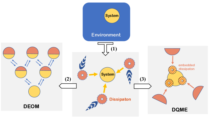
Figure 1: A schematic illustration of dissipaton equation of motion (DEOM) versus dissipatons–embedded quantum master equation (DQME). Block arrow (1) is a mapping that decomposes the original environment (blue square) into multiple dissipatons (red gears), conserving the hybridized correlation function. Dissipatons behave as quantum Brownian particles. Block arrow (2) represents the establishment of the DEOM of hierarchical structure. Each DDO (mixed red–yellow circle) incorporates a configuration of dissipatons. Block arrow (3) represents the establishment of the DQME, where the disspaton degrees of freedom are embedded into the system (dashed red vortex). Instead of a hierarchical structure, all the system–plus–dissipatons degrees of freedom are incorporated into a single dynamic equation, influenced by dissipaton Smoluchowski operators (red arches).

In this section, we will establish an equivalent dissipatons–embedded quantum master equation (DQME). This is concerned with the core system; i.e., the system–plus–dissipatons composite. First of all, there is a one–to–one correspondence between the dissipaton operators and real dimensionless variables:

$$\hat{f}_{k}/\zeta_{k}\xleftrightarrow{\text{effective}}x_{k}\in(-\infty,\infty),$$ (17)

where

$$\zeta_{k}\equiv\sqrt{(\eta_{k}+\eta^{*}_{\bar{k}})/2}\ \ \text{and}\ \ \xi_{k}\equiv\frac{\eta_{k}-\eta^{*}_{\bar{k}}}{2i\zeta_{k}}.$$ (18)

The “effective” correspondence means that the statistical characteristics of hybrid modes [cf. Eq. (13)] can be completely recovered by the moments of $\bm{x}\equiv\{x_{k}\}$; see Eq. (IV.2) and the discussions therein.

To proceed, we write the core–system distribution as

$$\hat{\rho}({\bm{x}},t)=\sum_{\bf n}\bigg{[}\rho_{\bf n}^{(n)}(t)\prod_{k}\phi_{n_{k}}(x_{k})\bigg{]},$$ (19)

with the dissipaton subspace basis functions,

$$\phi_{n_{k}}(x_{k})=(2\pi)^{-\frac{1}{4}}\frac{e^{-x^{2}_{k}/4}}{\zeta^{n_{k}}_{k}\sqrt{n_{k}!}}\phi_{n_{k}}^{\rm har}(x_{k}).$$ (20)

Involved are the standard harmonic oscillator wave functions,

$$\phi^{\rm har}_{n}(x)=(2\pi)^{-\frac{1}{4}}(2^{n}n!)^{-\frac{1}{2}}e^{-\frac{x^{2}}{4}}H_{n}\Big{(}\frac{x}{\sqrt{2}}\Big{)},$$ (21)

with $H_{n}(x)$ is the $n$th Hermite polynomial. The reason for choosing $\{\phi_{n}(x)\}$ as the basis will be discussed in the next section; see Eq. (IV.2) and the discussions therein. Due to the orthogonal relation:

$$\int\!\,e^{-x^{2}/2}H_{n}\Big{(}\frac{x}{\sqrt{2}}\Big{)}H_{n^{\prime}}\Big{(}\frac{x}{\sqrt{2}}\Big{)}{{\rm d}x}=(2\pi)^{\frac{1}{2}}2^{n}n!\delta_{nn^{\prime}},$$ (22)

we can then recast Eq. (19) as

$$\rho^{(n)}_{\bf n}(t)=\!\!\int\hat{\rho}({\bm{x}},t)\prod_{k}\bigg{[}\Big{(}\frac{\zeta_{k}}{\sqrt{2}}\Big{)}^{n_{k}}H_{n_{k}}\Big{(}\frac{x_{k}}{\sqrt{2}}\Big{)}\bigg{]}{\rm d}{\bm{x}}.$$ (23)

This is an alternative expression of DDOs, where ${\rm d}{\bm{x}}\equiv{\rm d}x_{1}\cdots{\rm d}x_{K}$.

By using Eq. (19) with DEOM (II.2), followed by some detailed algebra in Appendix A, we obtain the DQME,

$$\frac{\partial}{\partial t}\hat{\rho}({\bm{x}},t)= -i[H_{\mbox{\tiny S}},\hat{\rho}]+\sum_{k}\hat{\Gamma}_{k}\hat{\rho}-i\sum_{k}\zeta_{k}[\hat{Q},x_{k}\hat{\rho}]$$

$$-\sum_{k}\xi_{k}\Big{\{}\hat{Q},\frac{\partial\hat{\rho}}{\partial{x_{k}}}\Big{\}},$$ (24)

where

$$\hat{\Gamma}_{k}\equiv\gamma_{k}\frac{\partial}{\partial{x_{k}}}\Big{(}\frac{\partial}{\partial{x_{k}}}+x_{k}\Big{)}.$$ (25)

This is the generalized Smoluchowski operator and corresponds to the generalized diffusion equation (9); see also Eq. (A). The last two terms in Eq. (III) correspond to the generalized Wick’s theorem (11), describing the effect of system–bath coupling $H_{\mbox{\tiny S}\mbox{\tiny B}}$; see also Eqs. (A) and (A). It is worth reemphasizing that the parameters $\gamma_{k}$, $\zeta_{k}$ and $\xi_{k}$ can all be complex, whereas the variable $x_{k}$ is real. As also known, $\gamma_{\bar{k}}=\gamma^{\ast}_{k}$, $\zeta_{\bar{k}}=\zeta^{\ast}_{k}$ and $\xi_{\bar{k}}=\xi^{\ast}_{k}$; see Eq. (18), with $\bar{k}\in\{k=1,\cdots,K\}$.

Instead of a hierarchical structure, all the system–plus–dissipatons degrees of freedom are incorporated into a single dynamic equation; see Eq. (III), Fig. 1 and the remarks therein. It is worth noting that the methodology here is closely related to that in the Fokker–Planck theory, Zusman theory and the pseudomode method. Tan06082001 ; Dal01053813 ; Tam18030402 ; Tam19090402 ; Che19123035 ; Lam193721 ; Hu907078 The new DQME recovers the reduced system dynamics as specified by $\rho_{\mbox{\tiny S}}(t)$ without any approximation.

IV Statistical characteristics of dissipatons

IV.1 Dissipatons as generalized Brownian particles

In open quantum dynamics, the wave-particle duality of both system and hybrid bath plays important roles. In contrast to DEOM, DQME describes the influence of hybrid bath in the aspect of waves, with the picture of generalized Brownian particles for dissipatons. To this end, we consider

$${P}(\bm{x},t)\equiv{\rm tr}_{\mbox{\tiny S}}\hat{\rho}({\bm{x}},t),$$ (26)

and obtain

$$\frac{\partial}{\partial t}{P}(\bm{x},t)=\sum_{k}\hat{\Gamma}_{k}{P}(\bm{x},t)-\sum_{k}\frac{\partial}{\partial x_{k}}J_{k}(\bm{x},t),$$ (27)

with the last term the form of ${\bm{\nabla}}\cdot{\bm{J}}$, arising from the system–bath coupling. The dissipaton probability current density vector is given by

$$J_{k}(\bm{x},t)=2\xi_{k}{\rm tr}_{\mbox{\tiny S}}\big{[}\hat{Q}\hat{\rho}({\bm{x}},t)\big{]}.$$ (28)

Equation (27) provides a means to the statistics of hybrid bath. In particular, its equilibrium–state solution reads

$${P}^{\rm st}={\hat{\Gamma}}^{-1}{\bm{\nabla}}\cdot{\bm{J}}^{\rm st}.$$ (29)

with $\hat{\Gamma}=\sum_{k}\hat{\Gamma}_{k}$. However, to evaluate the current density, Eq. (28), $\hat{\rho}({\bm{x}},t)$ via DQME (III) is needed. From Eq. (29), we can derive the input–output relations involving dissipaton moments and dissipative system mode; see Appendix B.2 and comments therein. In the following, we will exploit the equivalent DEOM formalism to evaluate the hybrid bath statistics.

IV.2 Transient dissipaton moments

We will be interested in the expectation values of

$${\bm{x}}_{\bf n}^{(n)}\equiv x_{K}^{n_{K}}\cdots\ x_{1}^{n_{1}}.$$ (30)

To proceed, denote

$$\hat{X}^{(n)}_{\bf n}(t) \equiv\int{\bm{x}}^{(n)}_{\bf n}\,\hat{\rho}({\bm{x}},t)\,{\rm d}{\bm{x}},$$ (31)

and the transient dissipaton moments

$$\langle{\bm{x}}^{(n)}_{\bf n}(t)\rangle={\rm tr}_{\mbox{\tiny S}}\hat{X}^{(n)}_{\bf n}(t)=\int{\bm{x}}^{(n)}_{\bf n}\,{P}({\bm{x}},t)\,{\rm d}{\bm{x}}.$$ (32)

On the other hand, we have (see Appendix B)

$$\hat{X}^{(n)}_{\bf n}(t)=\sum_{\{m_{k}=0\}}^{\{\lfloor n_{k}/2\rfloor\}}c_{\bf nm}\rho^{(n-2m)}_{{\bf n}-2{\bf m}}(t),$$ (33)

where

$$\rho^{(n-2m)}_{{\bf n}-2{\bf m}}(t)\equiv{\rm tr}_{\mbox{\tiny B}}\big{[}\big{(}\hat{f}_{K}^{n_{K}-2m_{K}}\cdots\hat{f}_{1}^{n_{1}-2m_{1}}\big{)}^{\circ}\rho_{\mbox{\tiny T}}(t)\big{]},$$ (34)

and

$$c_{\bf nm}=\prod_{k=1}^{K}\frac{1}{\zeta^{n_{k}-2m_{k}}_{k}2^{m_{k}}}\frac{n_{k}!}{m_{k}!(n_{k}-2m_{k})!}.$$ (35)

We can recast Eq. (13) as [cf. Eq. (56) and discussion therein]

$$\quad\langle\hat{F}^{n}(t)\rangle =\!\int\!\Big{(}\sum_{k}\zeta_{k}x_{k}\Big{)}^{n}{{P}}(\bm{x},t)\,{\rm d}{\bm{x}}$$

$$=n!\sum_{\bf n}\Big{(}\prod_{k}\frac{\zeta^{n_{k}}_{k}}{n_{k}!}\Big{)}\langle{\bm{x}}^{(n)}_{\bf n}(t)\rangle.$$ (36)

This also implies the one–to–one correspondence between the dissipaton operators and real dimensionless variables, as specified in Eq. (17).

V Numerical Demonstrations

For demonstration, we consider the electron transfer model, Han0611438 ; Che07438

$$\!\!\!H_{\mbox{\tiny S}}=(\epsilon+\lambda)|1\rangle\langle 1|+V(|1\rangle\langle 0|+|0\rangle\langle 1|),$$ (37)

with the dissipative system mode $\hat{Q}=-|1\rangle\langle 1|$. Here, $|0\rangle$ is the donor state and $|1\rangle$ is the acceptor state, with the energy bias $\epsilon$, the interstate coupling $V$ and the solvent reorganization energy $\lambda$. The latter arises from the bath spectral density, which takes the Brownian oscillator model, Yan05187

$$J_{\mbox{\tiny B}}(\omega)=\frac{2\lambda\omega^{2}_{0}\zeta\omega}{(\omega^{2}-\omega_{0}^{2})^{2}+\omega^{2}\zeta^{2}}.$$ (38)

Here in the scene of electron transfer, the hybrid mode $\hat{F}(t)$ is interpreted as “solvation coordinate” along the elecron transfer. Its expectation $\langle\hat{F}(t)\rangle$ and standard deviation $\sigma_{F}={\langle\hat{F}^{2}(t)\rangle^{1/2}}$ measure the reaction progress and the width of solvent wavepackage, respectively.

The influence of anharmonic system induces the non-Gaussian dynamics of the environments. To measure the non-Gaussianity of a distribution, there are two basic dimensionless quantities: (Sha15, ) the skewness $K_{3}/\sigma^{3}_{F}$ and the kurtosis $K_{4}/\sigma^{4}_{F}$. They characterize the asymmetry and the tailedness, respectively, in terms of the $n$th cumulant,

$$K_{n}(t)=\langle\hat{F}^{n}(t)\rangle-\sum^{n-1}_{m=1}{n-1\choose m}K_{n-m}(t)\langle\hat{F}^{m}(t)\rangle,$$ (39)

with $K_{1}(t)=\langle\hat{F}(t)\rangle$.

Figure 2 depicts the results of calculating the statistical characteristics of transient hybrid mode $\hat{F}(t)$ at different coupling strength, i.e. the reorganization energy $\lambda$. We can see that all the characteristics of $\hat{F}(t)$ oscillate at the frequency about $\Omega_{\mbox{\tiny S}}=\sqrt{\epsilon^{2}+4V^{2}}$, the characteristic frequency of system, in short time evolution and converge to steady values in the long time asymptotic regime.

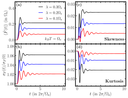
Figure 2: Statistical characteristics of hybrid mode $\hat{F}(t)$ at three specified $\lambda$ and the given temperature, where $\Omega_{\mbox{\tiny S}}=\sqrt{\epsilon^{2}+4V^{2}}$: (a) The mean value; (b) The standard deviation $\sigma_{F}(t)/\sigma_{F}(0)$; (c) The skewness $K_{3}/\sigma^{3}_{F}$; (d) The kurtosis $K_{4}/\sigma^{4}_{F}$. Other parameters are $V=0.4,\,\omega_{0}=\zeta=1$ in unit of $\Omega_{\mbox{\tiny S}}$.

As the coupling strengthens, the mean value and the standard deviation increase, measuring the drifting and widening of distribution of reaction coordinate, respectively. The skewness and kurtosis of hybrid mode deviate further from 0 as coupling strengthens, that indicates the influence of the anharmonic system violates the Gaussianity of the environment.

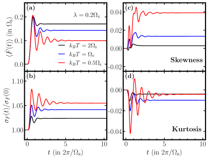
Figure 3: Statistical characteristics of hybrid mode $\hat{F}(t)$ at three specified temperatures and the given $\lambda$, where $\Omega_{\mbox{\tiny S}}=\sqrt{\epsilon^{2}+4V^{2}}$: (a) The mean value; (b) The standard deviation $\sigma_{F}(t)/\sigma_{F}(0)$; (c) The skewness $K_{3}/\sigma^{3}_{F}$; (d) The kurtosis $K_{4}/\sigma^{4}_{F}$. Other parameters are $V=0.4,\,\omega_{0}=\zeta=1$ in unit of $\Omega_{\mbox{\tiny S}}$.

Figure 3 shows the transient evolutions of statistical characteristics of the hybrid mode at different temperatures. Similar dynamical oscillation behaviors as that in Fig. 2 are displayed. On the other hand, when temperature increases, $\langle\hat{F}\rangle$ at the steady state increases (cf. Fig. 3a), while $\sigma_{F}(t)/\sigma_{F}(0)$ and the skewness reduce (cf. Fig. 3b and 3c). However, the kurtosis does not varies monotunously in this regime, which suggests the complicated behaviors of the tailedness of relevant distributions.

VI Concluding remarks

To summarize, in this work we construct the dissipaton–embedded quantum master equation (DQME) from the DEOM theory via introducing the one–to–one correspondence between the dissipaton operators and real dimensionless variables. Instead of a hierarchical structure, all the system–plus–dissipatons degrees of freedom are incorporated into a single dynamic equation in DQME. The new DQME recovers the reduced system dynamics as specified by $\rho_{\mbox{\tiny S}}(t)$ without any approximation. Moreover, the statistical characteristics of hybrid modes can be completely recovered.

The formalism of DQME reveals the picture of dissipatons as the Brownian quasi-particles interacting with the system. Based on the DQME, we can discuss the evolution of dissipaton distribution under the influence of system and correlate the transient moments of dissipatons with DDOs.

The fermionic DQME can also been readily established in a similar manner, which would benefit for the simulations on such as spintronic and superconductive systems. The DQME formalism brings the possibility of achieving the quantum simulation of non-Markovian open quantum dynamics. Since all the dissipaton degrees of freedom are represented by continuous real variables in DQME, this makes it a versatile formalism for incorporating matrix product states, real–space renormalization group, and other numerical methods. It is anticipated that DQME developed in this work would become an important tool for quantum mechanics of open systems.

Appendix A Derivation of DQME (III)

For later use, we first rewrite Eq. (19) as

$$\hat{\rho}({\bm{x}},t)=\sum_{\bf n}\bigg{[}\tilde{\rho}_{\bf n}^{(n)}(t)\prod_{k}\tilde{\phi}_{n_{k}}(x_{k})\bigg{]},$$ (40)

with

$$\tilde{\rho}_{\bf n}^{(n)}(t)=\rho_{\bf n}^{(n)}(t)\Big{/}\prod_{k}\zeta^{n_{k}}_{k},$$ (41)

and

$$\tilde{\phi}_{n_{k}}(x_{k})=(2\pi)^{-\frac{1}{4}}\frac{e^{-x^{2}_{k}/4}}{\sqrt{n_{k}!}}\phi_{n_{k}}^{\rm har}(x_{k}).$$ (42)

Note for $\tilde{\phi}_{n}(x)$, we have Shi09164518

$$x\tilde{\phi}_{n}(x)=\tilde{\phi}_{n-1}(x)+(n+1)\tilde{\phi}_{n+1}(x),$$ (43)

and

$$\frac{\partial\tilde{\phi}_{n}(x)}{\partial{x}}=-(n+1)\tilde{\phi}_{n+1}(x).$$ (44)

According to DEOM (II.2), the EOM for $\tilde{\rho}_{\bf n}^{(n)}(t)$ reads

$$\dot{\tilde{\rho}}^{(n)}_{\bf{n}}(t)= -\Big{(}{i\cal{L}}_{\mbox{\tiny S}}+\sum_{k}{n_{k}}\gamma_{k}\Big{)}\tilde{\rho}^{(n)}_{{\bf n}}(t)$$

$$-i\sum_{k}\zeta_{k}\hat{Q}^{\times}\Big{[}\tilde{\rho}^{(n+1)}_{{\bf n}^{+}_{k}}(t)+n_{k}\tilde{\rho}^{(n-1)}_{{\bf n}^{-}_{k}}(t)\Big{]}$$

$$+\sum_{k}n_{k}\xi_{k}\hat{Q}^{\diamond}\tilde{\rho}^{(n-1)}_{{\bf n}^{-}_{k}}(t),$$ (45)

where Eq. (18) is used and $\hat{A}^{\diamond}\rho\equiv\hat{A}\rho+\rho\hat{A}$. With

$$\sum_{\bf n}\sum_{k}{n_{k}}\gamma_{k}\tilde{\rho}^{(n)}_{{\bf n}}\prod_{j}\tilde{\phi}_{n_{j}}(x_{j})$$

$$= -\sum_{k}\gamma_{k}\frac{\partial}{\partial x_{k}}(x_{k}+\frac{\partial}{\partial x_{k}})\sum_{\bf n}\tilde{\rho}^{(n)}_{\bf n}\prod_{j}\tilde{\phi}_{n_{j}}(x_{j})$$

$$= -\sum_{k}\gamma_{k}\frac{\partial}{\partial x_{k}}(x_{k}+\frac{\partial}{\partial x_{k}})\hat{\rho}({\bm{x}}),$$ (46)

$$\sum_{\bf n}\bigg{[}\Big{(}\tilde{\rho}_{{\bf n}_{k}^{+}}^{(n+1)}+n_{k}\tilde{\rho}_{{\bf n}_{k}^{-}}^{(n-1)}\Big{)}\prod_{j}\tilde{\phi}_{n_{j}}(x_{j})\bigg{]}$$

$$= \sum_{\bf n}\bigg{[}\tilde{\rho}_{{\bf n}}^{(n)}\prod_{j}\big{[}\tilde{\phi}_{n_{j}-\delta_{kj}}(x_{j})+(n_{k}+1)\phi_{n_{j}+\delta_{kj}}(x_{j})\big{]}\bigg{]}$$

$$= x_{k}\hat{\rho}({\bm{x}}),$$ (47)

and

$$\sum_{\bf n}n_{k}\tilde{\rho}_{{\bf n}_{k}^{-}}^{(n-1)}\prod_{j}\tilde{\phi}_{n_{j}}(x_{j})$$

$$= -\sum_{\bf n}\tilde{\rho}_{{\bf n}_{k}^{-}}^{(n-1)}\frac{\partial}{\partial x_{k}}\prod_{j}\tilde{\phi}_{n_{j}-\delta_{kj}}(x_{j})$$

$$= -\frac{\partial}{\partial x_{k}}\hat{\rho}({\bm{x}}),$$ (48)

we then obtain the DQME (III) from Eq. (A) together with Eqs. (A)–(A).

Appendix B Moments of dissipatons

B.1 Basic relations and transient dissipaton moments

Let us start with some basic relations:

$$\langle\hat{F}_{\mbox{\tiny B}}^{2}\rangle_{\mbox{\tiny B}}=\sum_{k}\eta_{k}=\sum_{k}\eta_{\bar{k}}^{\ast}=\sum_{k}\zeta_{k}^{2}.$$ (49)

Applied here are Eqs. (4a), (4b) and (18). Moreover,

$${\bm{x}}_{\bf n}^{(n)}\frac{\partial}{\partial x_{k}}=\frac{\partial}{\partial x_{k}}{\bm{x}}_{\bf n}^{(n)}-n_{k}{\bm{x}}_{{\bf{n}}^{-}_{k}}^{(n-1)},$$ (50)

and [cf. Eq. (25)]

$${\bm{x}}_{\bf n}^{(n)}\hat{\Gamma}_{k} =\gamma_{k}\bigg{[}\Big{(}\frac{\partial^{2}}{\partial x^{2}_{k}}-n_{k}\Big{)}{\bm{x}}_{\bf n}^{(n)}+n_{k}(n_{k}-1){\bm{x}}_{{\bf{n}}^{--}_{kk}}^{(n-2)}$$

$$\quad-n_{k}\frac{\partial}{\partial x_{k}}{\bm{x}}_{{\bf{n}}^{-}_{k}}^{(n-1)}+\frac{\partial}{\partial x_{k}}{\bm{x}}_{{\bf{n}}^{+}_{k}}^{(n+1)}\bigg{]}.$$ (51)

With the relation

$$\Big{(}\frac{x}{\sqrt{2}}\Big{)}^{n}=\frac{n!}{2^{n}}\sum^{\lfloor n/2\rfloor}_{m}\frac{1}{m!(n-2m)!}H_{n-2m}\Big{(}\frac{x}{\sqrt{2}}\Big{)},$$ (52)

we can obtain $\hat{X}^{(n)}_{\bf n}$ in Eq. (31)

$$\hat{X}^{(n)}_{\bf n}=\int\,{\bm{x}}^{(n)}_{\bf n}\rho(t;\{x_{k}\}){\rm d}{\bm{x}}=\!\!\sum^{\{[n_{k}/2]\}}_{\{m_{k}\}}\!\!c_{\bf mn}\rho^{(n-2m)}_{\bf{n}-2\bf{m}},$$ (53)

expressed by DDOs, where $c_{\bf mn}$ is given in Eq. (35). Inversely, we have

$$\rho^{(n)}_{\bf n}(t)=\sum_{\{m_{k}=0\}}^{\{\lfloor n_{k}/2\rfloor\}}\bar{c}_{\bf nm}\hat{X}^{(n-2m)}_{\bf{n}-2\bf{m}}(t),$$ (54)

with

$$\bar{c}_{\bf nm}=\prod_{k}\zeta^{n_{k}}_{k}2^{-m_{k}}\frac{(-1)^{m_{k}}n_{k}!}{m_{k}!(n_{k}-2m_{k})!}.$$ (55)

To show that Eq. (IV.2) is equivalent Eq. (13), we first rewrite Eq. (13) as

$$\!\!\langle\hat{F}^{n}\rangle= \sum_{m=0}^{\lfloor n/2\rfloor}\frac{n!}{2^{m}m!}\langle{\hat{F}}_{\mbox{\tiny B}}^{2}\rangle_{\mbox{\tiny B}}^{m}\sideset{}{{}^{\prime}}{\sum}_{\{n_{k}-2m_{k}\}}\frac{1}{n_{1}!\cdots n_{K}!}{\rm tr_{\mbox{\tiny S}}}\rho^{(n-2m)}_{\bf n-2m}.$$ (56)

By further using the last identity in Eq. (49), we then reproduce Eq. (13). This validates the effective mapping (17), which conserve the statistics of the hybrid bath.

B.2 Equilibrium dissipaton statistics

To obtain $\langle{\bm{x}}_{\bf n}^{(n)}\rangle$, the moments of $\{x_{k}\}$ at thermal equilibrium, we first recast Eq. (29) as

$$\int{\bm{x}}_{\bf n}^{(n)}\,{\hat{\Gamma}}{P}^{\rm st}\,{\rm d}{\bm{x}}=\int{\bm{x}}_{\bf n}^{(n)}{\bm{\nabla}}\cdot{\bm{J}}^{\rm st}\,{\rm d}{\bm{x}}.$$ (57)

For Eq. (30), Eqs. (50) and (B.1) gives the input–output relation reading

$$\!\!\langle{\bm{x}}^{(n)}_{\bf n}\rangle\!=\!\frac{2}{\gamma_{\bf n}^{(n)}}\!\sum_{k}\bigg{[}\xi_{k}n_{k}\langle\hat{Q}{\bm{x}}^{(n-1)}_{{\bf n}_{k}^{-}}\rangle+\gamma_{k}{n_{k}\choose 2}\langle{\bm{x}}^{(n-2)}_{{\bf n}_{kk}^{--}}\rangle\bigg{]},$$ (58)

where $\gamma_{\bf n}^{(n)}\equiv\sum_{k}n_{k}\gamma_{k}$.

To close the input–output relation, one may further consider for any operator $\hat{A}$, there exists the relation

$$\quad-i\langle[H_{\mbox{\tiny S}},\hat{A}]{\bm{x}}^{(n)}_{\bf n}\rangle+\sum_{k}\xi_{k}n_{k}\langle\{\hat{A},\hat{Q}\}{\bm{x}}_{{\bf n}^{-}_{k}}^{(n-1)}\rangle$$

$$=\sum_{k}\gamma_{k}\Big{[}n_{k}\langle\hat{A}{\bm{x}}_{\bf n}^{(n)}\rangle-n_{k}(n_{k}-1)\langle\hat{A}{\bm{x}}_{{\bf n}^{--}_{kk}}^{(n-2)}\rangle\Big{]}.$$ (59)

It is evident that the recurrence relation is closed when $\hat{A}$ belongs to a linear space $\mathbb{L}$ of operators. Here, the linearly independent basis set of $\mathbb{L}$ has two parts: (i) basis vectors $\hat{V}$ satisfying $[H_{\mbox{\tiny S}},\hat{V}]=0$ and $\{\hat{Q},\hat{V}\}=0$; (ii) finite basis vectors generated from the identical operator $\hat{I}$ via the operation $\{\hat{Q},\cdot\,\}$ and $[H_{\mbox{\tiny S}},\cdot\,]$. As a result, the basis set is $\{\hat{I},\hat{Q},[H_{\mbox{\tiny S}},\hat{Q}],\hat{Q}^{2},[H_{\mbox{\tiny S}},[H_{\mbox{\tiny S}},\hat{Q}]],\{\hat{Q},[H_{\mbox{\tiny S}},\hat{Q}]\},\cdots\}$.Gu851310

For example, for the spin–boson system where $H_{\mbox{\tiny S}}=\hat{\sigma}_{x}$, $\hat{Q}=\hat{\sigma}_{z}$, the linearly dependent basis of $\mathbb{L}$ is $\{\hat{I},\hat{\sigma}_{z},\hat{\sigma}_{y},\hat{\sigma}_{x}\}$, since $[\hat{\sigma}_{i},\hat{\sigma}_{j}]=2i\varepsilon_{ijk}\hat{\sigma}_{k}$ and $\{\hat{\sigma}_{i},\hat{\sigma}_{j}\}=2\delta_{ij}\hat{I}$. Then, when $\hat{A}=\hat{\sigma}_{x}$, $\hat{\sigma}_{y}$ and $\hat{\sigma}_{z}$, we have

$$0=\sum_{k}\gamma_{k}\Big{[}n_{k}\langle\hat{\sigma}_{x}{\bm{x}}_{\bf n}^{(n)}\rangle-n_{k}(n_{k}-1)\langle\hat{\sigma}_{x}{\bm{x}}_{{\bf n}^{--}_{kk}}^{(n-2)}\rangle\Big{]},$$ (60)

$$2\langle\hat{\sigma}_{z}{\bm{x}}^{(n)}_{\bf n}\rangle=\sum_{k}\gamma_{k}\Big{[}n_{k}\langle\hat{\sigma}_{y}{\bm{x}}_{\bf n}^{(n)}\rangle-n_{k}(n_{k}-1)\langle\hat{\sigma}_{y}{\bm{x}}_{{\bf n}^{--}_{kk}}^{(n-2)}\rangle\Big{]},$$ (61)

and

$$\quad 2\langle\hat{\sigma}_{y}{\bm{x}}^{(n)}_{\bf n}\rangle-2\sum_{k}\xi_{k}n_{k}\langle\hat{\sigma}_{z}{\bm{x}}_{{\bf n}^{-}_{k}}^{(n-1)}\rangle$$

$$=-\sum_{k}\gamma_{k}\Big{[}n_{k}\langle\hat{\sigma}_{z}{\bm{x}}_{\bf n}^{(n)}\rangle-n_{k}(n_{k}-1)\langle\hat{\sigma}_{z}{\bm{x}}_{{\bf n}^{--}_{kk}}^{(n-2)}\rangle\Big{]},$$ (62)

separately.

References

• (1) U. Weiss, Quantum Dissipative Systems, World Scientific, Singapore, 2021, 5th ed.
• (2) H. P. Breuer and F. Petruccione, The Theory of Open Quantum Systems, Oxford University Press, New York, 2002.
• (3) Y. J. Yan and R. X. Xu, “Quantum mechanics of dissipative systems,” Annu. Rev. Phys. Chem. 56, 187 (2005).
• (4) W. H. Louisell, Quantum Statistical Properties of Radiation, Wiley, New York, 1973.
• (5) C. P. Slichter, Principles of Magnetic Resonance, Springer Verlag, New York, 1990.
• (6) L. M. K. Vandersypen and I. L. Chuang, “NMR techniques for quantum control and computation,” Rev. Mod. Phys. 76, 1037 (2005).
• (7) C. F. Klingshirn, Semiconductor Optics, Springer-Verlag, Heidelberg, 1997.
• (8) J. Rammer, Quantum Transport Theory, Perseus Books, Reading, Mass., 1998.
• (9) Y. Akamatsu, “Heavy quark master equations in the Lindblad form at high temperatures,” Phys. Rev. D 91, 056002 (2015).
• (10) S. Mukamel, “Reduced equations of motion for collisionless molecular multiphoton processes,” Adv. Chem. Phys. 47, 509 (1981).
• (11) Y. J. Yan and S. Mukamel, “Electronic dephasing, vibrational relaxation, and solvent friction in molecular nonlinear optical lineshapes,” J. Chem. Phys. 89, 5160 (1988).
• (12) Y. J. Yan and S. Mukamel, “Photon echoes of polyatomic molecules in condensed phases,” J. Chem. Phys. 94, 179 (1991).
• (13) V. Chernyak and S. Mukamel, “Collective coordinates for nuclear spectral densities in energy transfer and femtosecond spectroscopy of molecular aggregates,” J. Chem. Phys. 105, 4565 (1996).
• (14) Y. Tanimura and S. Mukamel, “Two-dimensional femtosecond vibrational spectroscopy of liquids,” J. Chem. Phys. 99, 9496 (1993).
• (15) Y. Tanimura and S. Mukamel, “Multistate quantum Fokker-Planck approach to nonadiabatic wave packet dynamics in pump-probe spectroscopy,” J. Chem. Phys. 101, 3049 (1994).
• (16) K. E. Dorfman, D. V. Voronine, S. Mukamel, and M. O. Scully, “Photosynthetic reaction center as a quantum heat engine,” Proc. Natl. Acad. Sci. 110, 2746 (2013).
• (17) S. Kundu, R. Dani, and N. Makri, “B800-to-B850 relaxation of excitation energy in bacterial light harvesting: All-state, all-mode path integral simulations,” J. Chem. Phys. 157, 015101 (2022).
• (18) Y. Tanimura and R. Kubo, “Time evolution of a quantum system in contact with a nearly Gaussian-Markovian noise bath,” J. Phys. Soc. Jpn. 58, 101 (1989).
• (19) Y. Tanimura, “Nonperturbative expansion method for a quantum system coupled to a harmonic-oscillator bath,” Phys. Rev. A 41, 6676 (1990).
• (20) Y. Tanimura, “Stochastic Liouville, Langevin, Fokker-Planck, and master equation approaches to quantum dissipative systems,” J. Phys. Soc. Jpn. 75, 082001 (2006).
• (21) Y. A. Yan, F. Yang, Y. Liu, and J. S. Shao, “Hierarchical approach based on stochastic decoupling to dissipative systems,” Chem. Phys. Lett. 395, 216 (2004).
• (22) R. X. Xu, P. Cui, X. Q. Li, Y. Mo, and Y. J. Yan, “Exact quantum master equation via the calculus on path integrals,” J. Chem. Phys. 122, 041103 (2005).
• (23) R. X. Xu and Y. J. Yan, “Dynamics of quantum dissipation systems interacting with bosonic canonical bath: Hierarchical equations of motion approach,” Phys. Rev. E 75, 031107 (2007).
• (24) Y. Tanimura, “Numerically “exact” approach to open quantum dynamics: The hierarchical equations of motion (HEOM),” J. Chem. Phys 153, 020901 (2020).
• (25) J. S. Shao, “Decoupling quantum dissipation interaction via stochastic fields,” J. Chem. Phys. 120, 5053 (2004).
• (26) C.-Y. Hsieh and J. Cao, “A unified stochastic formulation of dissipative quantum dynamics. II. Beyond linear response of spin baths,” J. Chem. Phys. 148, 014104 (2018).
• (27) I. Imry, Introduction to Mesoscopic Physics, Oxford university press, 2002.
• (28) H. Haug and A.-P. Jauho, Quantum Kinetics in Transport and Optics of Semiconductors, Springer-Verlag, Berlin, 2nd, substantially revised edition, 2008, Springer Series in Solid-State Sciences 123.
• (29) H. D. Zhang, R. X. Xu, X. Zheng, and Y. J. Yan, “Nonperturbative spin-boson and spin-spin dynamics and nonlinear Fano interferences: A unified dissipaton theory based study,” J. Chem. Phys. 142, 024112 (2015).
• (30) P. L. Du, Y. Wang, R. X. Xu, H. D. Zhang, and Y. J. Yan, “System-bath entanglement theorem with Gaussian environments,” J. Chem. Phys. 152, 034102 (2020).
• (31) Z. H. Chen, Y. Wang, R. X. Xu, and Y. J. Yan, “Correlated vibration-solvent effects on the non-Condon exciton spectroscopy,” J. Chem. Phys. 154, 244105 (2021).
• (32) Y. Meir and N. S. Wingreen, “Landauer formula for the current through an interacting electron region,” Phys. Rev. Lett. 68, 2512 (1992).
• (33) D. Gruss, K. A. Velizhanin, and M. Zwolak, “Landauer’s formula with finite-time relaxation: Kramers’ crossover in electronic transport,” Phys. Rep. 6, 24514 (2016).
• (34) Y. Wang, R. X. Xu, and Y. J. Yan, “Entangled system-and-environment dynamics: Phase-space dissipaton theory,” J. Chem. Phys. 152, 041102 (2020).
• (35) P. L. Du, Z. H. Chen, Y. Su, Y. Wang, R. X. Xu, and Y. J. Yan, “Nonequilibrium system–bath entanglement theorem versus heat transport,” Chem. J. Chin. Univ. 42, 2155 (2021).
• (36) Y. Wang, Z. H. Chen, R. X. Xu, X. Zheng, and Y. J. Yan, “A statistical quasi–particles thermofield theory with Gaussian environments: System–bath entanglement theorem for nonequilibrium correlation functions,” J. Chem. Phys. 157, 044012 (2022).
• (37) J. G. Kirkwood, “Statistical mechanics of fluid mixtures,” J. Chem. Phys. 3, 300 (1935).
• (38) H. Gong, Y. Wang, H. D. Zhang, Q. Qiao, R. X. Xu, X. Zheng, and Y. J. Yan, “Equilibrium and transient thermodynamics: A unified dissipaton–space approach,” J. Chem. Phys. 153, 154111 (2020).
• (39) H. Gong, Y. Wang, H. D. Zhang, R. X. Xu, X. Zheng, and Y. J. Yan, “Thermodynamic free–energy spectrum theory for open quantum systems,” J. Chem. Phys. 153, 214115 (2020).
• (40) Y. J. Yan, “Theory of open quantum systems with bath of electrons and phonons and spins: Many-dissipaton density matrixes approach,” J. Chem. Phys. 140, 054105 (2014).
• (41) Y. J. Yan, J. S. Jin, R. X. Xu, and X. Zheng, “Dissipaton equation of motion approach to open quantum systems,” Frontiers Phys. 11, 110306 (2016).
• (42) Y. Wang and Y. J. Yan, “Quantum mechanics of open systems: Dissipaton theories,” J. Chem. Phys. 157, 170901 (2022).
• (43) R. X. Xu, H. D. Zhang, X. Zheng, and Y. J. Yan, “Dissipaton equation of motion for system-and-bath interference dynamics,” Sci. China Chem. 58, 1816 (2015), Special Issue: Lemin Li Festschrift.
• (44) H. D. Zhang, Q. Qiao, R. X. Xu, and Y. J. Yan, “Effects of Herzberg–Teller vibronic coupling on coherent excitation energy transfer,” J. Chem. Phys. 145, 204109 (2016).
• (45) R. X. Xu, Y. Liu, H. D. Zhang, and Y. J. Yan, “Theory of quantum dissipation in a class of non-Gaussian environments,” Chin. J. Chem. Phys. 30, 395 (2017).
• (46) R. X. Xu, Y. Liu, H. D. Zhang, and Y. J. Yan, “Theories of quantum dissipation and nonlinear coupling bath descriptors,” J. Chem. Phys. 148, 114103 (2018).
• (47) Y. Su, Z. H. Chen, H.-J. Zhu, Y. Wang, L. Han, R. X. Xu, and Y. J. Yan, “Electron transfer under the Floquet modulation in donor–bridge–acceptor systems,” J. Phys. Chem. A 126, 4554 (2022).
• (48) H. Gong, Y. Wang, X. Zheng, R. X. Xu, and Y. J. Yan, “Nonequilibrium work distributions in quantum impurity system–bath mixing processes,” J. Chem. Phys. 157, 054109 (2022).
• (49) Z. H. Chen, Y. Wang, R. X. Xu, and Y. J. Yan, “Quantum dissipation with nonlinear environment couplings: Stochastic fields dressed dissipaton equation of motion approach,” J. Chem. Phys. 155, 174111 (2021).
• (50) H. D. Zhang, R. X. Xu, X. Zheng, and Y. J. Yan, “Statistical quasi-particle theory for open quantum systems,” Mol. Phys. 116, 780 (2018), Special Issue, “Molecular Physics in China”.
• (51) J. Hu, R. X. Xu, and Y. J. Yan, “Padé spectrum decomposition of Fermi function and Bose function,” J. Chem. Phys. 133, 101106 (2010).
• (52) J. Hu, M. Luo, F. Jiang, R. X. Xu, and Y. J. Yan, “Padé spectrum decompositions of quantum distribution functions and optimal hierarchial equations of motion construction for quantum open systems,” J. Chem. Phys. 134, 244106 (2011).
• (53) J. J. Ding, J. Xu, J. Hu, R. X. Xu, and Y. J. Yan, “Optimized hierarchical equations of motion for Drude dissipation with applications to linear and nonlinear optical responses,” J. Chem. Phys. 135, 164107 (2011).
• (54) J. J. Ding, R. X. Xu, and Y. J. Yan, “Optimizing hierarchical equations of motion for quantum dissipation and quantifying quantum bath effects on quantum transfer mechanisms,” J. Chem. Phys. 136, 224103 (2012).
• (55) X. Zheng, R. X. Xu, J. Xu, J. S. Jin, J. Hu, and Y. J. Yan, “Hierarchical equations of motion for quantum dissipation and quantum transport,” Prog. Chem. 24, 1129 (2012).
• (56) Z. H. Chen, Y. Wang, X. Zheng, R. X. Xu, and Y. J. Yan, “Universal time-domain Prony fitting decomposition for optimized hierarchical quantum master equations,” J. Chem. Phys. 156, 221102 (2022).
• (57) L. Cui, H. D. Zhang, X. Zheng, R. X. Xu, and Y. J. Yan, “Highly efficient and accurate sum–over–poles expansion of Fermi and Bose functions at near zero temperatures: Fano spectrum decomposition scheme,” J. Chem. Phys. 151, 024110 (2019).
• (58) H. D. Zhang, L. Cui, H. Gong, R. X. Xu, X. Zheng, and Y. J. Yan, “Hierarchical equations of motion method based on Fano spectrum decomposition for low temperature environments,” J. Chem. Phys. 152, 064107 (2020).
• (59) Y. Zhou and J. S. Shao, “Solving the spin-boson model of strong dissipation with flexible random-deterministic scheme,” J. Chem. Phys. 128, 034106 (2008).
• (60) H. Liu, L. L. Zhu, S. M. Bai, and Q. Shi, “Reduced quantum dynamics with arbitrary bath spectral densities: Hierarchical equations of motion based on several different bath decomposition schemes,” J. Chem. Phys. 140, 134106 (2014).
• (61) Z. F. Tang, X. L. Ouyang, Z. H. Gong, H. B. Wang, and J. L. Wu, “Extended hierarchy equation of motion for the spin-boson model,” J. Chem. Phys. 143, 224112 (2015).
• (62) K. Nakamura and Y. Tanimura, “Hierarchical Schrödinger equations of motion for open quantum dynamics,” Phys. Rev. A 98, 012109 (2018).
• (63) T. Ikeda and G. D. Scholes, “Generalization of the hierarchical equations of motion theory for efficient calculations with arbitrary correlation functions,” J. Chem. Phys. 152, 204101 (2020).
• (64) N. Lambert, S. Ahmed, M. Cirio, and F. Nori, “Modelling the ultra-strongly coupled spin-boson model with unphysical modes,” Nature Comm. 10, 3721 (2019).
• (65) R. P. Feynman and F. L. Vernon, Jr., “The theory of a general quantum system interacting with a linear dissipative system,” Ann. Phys. 24, 118 (1963).
• (66) L. L. Zhu, H. Liu, W. W. Xie, and Q. Shi, “Explicit system-bath correlation calculated using the hierarchical equations of motion method,” J. Chem. Phys. 137, 194106 (2012).
• (67) B. J. Dalton, S. M. Barnett, and B. M. Garraway, “Theory of pseudomodes in quantum optical processes,” Phys. Rev. A 64, 053813 (2001).
• (68) D. Tamascelli, A. Smirne, S. F. Huelga, and M. B. Plenio, “Nonperturbative treatment of non-Markovian dynamics of open quantum systems,” Phys. Rev. Lett. 120, 030402 (2018).
• (69) D. Tamascelli, A. Smirne, J. Lim, S. F. Huelga, and M. B. Plenio, “Efficient simulation of finite-temperature open quantum systems,” Phys. Rev. Lett. 123, 090402 (2019).
• (70) F. Chen, E. Arrigoni, and M. Galperin, “Markovian treatment of non-Markovian dynamics of open Fermionic systems,” New J. Phys. 21, 123035 (2019).
• (71) H. Gang and H. Haken, “Steepest-descent approximation of stationary probability distribution of systems driven by weak colored noise,” Phys. Rev. A 41, 7078 (1990).
• (72) P. Han, R. X. Xu, B. Q. Li, J. Xu, P. Cui, Y. Mo, and Y. J. Yan, “Kinetics and thermodynamics of electron transfer in Debye solvents: An analytical and nonperturbative reduced density matrix theory,” J. Phys. Chem. B 110, 11438 (2006).
• (73) Y. Chen, R. X. Xu, H. W. Ke, and Y. J. Yan, “Electron transfer theory revisit: Motional narrowing induced non-Markovian rate processes,” Chin. J. Chem. Phys. 20, 438 (2007).
• (74) R. Shanmugam and R. Chattamvelli, “Skewness and Kurtosis,” in Statistics for Scientists and Engineers, chapter 4, pages 89–110, John Wiley & Sons, Ltd, 2015.
• (75) Q. Shi, L. P. Chen, G. J. Nan, R. X. Xu, and Y. J. Yan, “Electron transfer dynamics: Zusman equation versus exact theory,” J. Chem. Phys. 130, 164518 (2009).
• (76) Y. Gu, “Group-theoretical formalism of quantum mechanics based on quantum generalization of characteristic functions,” Phys. Rev. A 32, 1310 (1985).