Abstract

Recently, mean field control (MFC) has provided a tractable and theoretically founded approach to otherwise difficult cooperative multi-agent control. However, the strict assumption of many independent, homogeneous agents may be too stringent in practice. In this work, we propose a novel discrete-time generalization of Markov decision processes and MFC to both many minor agents and potentially complex major agents – major-minor mean field control (M3FC). In contrast to deterministic MFC, M3FC allows for stochastic minor agent distributions with strong correlation between minor agents through the major agent state, which can model arbitrary problem details not bound to any agent. Theoretically, we give rigorous approximation properties with novel proofs for both M3FC and existing MFC models in the finite multi-agent problem, together with a dynamic programming principle for solving such problems. In the infinite-horizon discounted case, existence of an optimal stationary policy follows. Algorithmically, we propose the major-minor mean field proximal policy optimization algorithm (M3FPPO) as a novel multi-agent reinforcement learning algorithm and demonstrate its success in illustrative M3FC-type problems.

1 Introduction

Recent successes of reinforcement learning (RL) Vinyals et al. (2019); Schrittwieser et al. (2020); Ouyang et al. (2022) motivate the search for according techniques in the multi-agent case, aptly referred to as multi-agent reinforcement learning (MARL). Due to the complexity of many-agent control problems Bernstein et al. (2002); Daskalakis et al. (2009), a common approach is to exploit problem structure in order to achieve principled, scalable solutions. In this work, we consider systems with many agents, interacting through aggregated information – referred to as mean field – of all agents. Indeed, in practice such aggregation is often found on some level, in e.g. chemical reaction networks where molecules are summarized into their aggregate mass Anderson & Kurtz (2011), related mass-action epidemics models where infection rates scale with the infected Kiss et al. (2017), or traffic where congestion depends on the number of cars on a road Cabannes et al. (2022).

Mean field games and control.

Control in aggregated interaction models is often considered by the study of mean field games (MFG) and control (MFC), where agents interact only through their empirical distribution. Since the introduction of stochastic differential MFGs Huang et al. (2006); Lasry & Lions (2007), the concept has been studied in various forms, ranging from partial observability Saldi et al. (2019); Şen & Caines (2019) over learning solutions Guo et al. (2019); Perrin et al. (2020); Cui & Koeppl (2021); Guo et al. (2022); Pérolat et al. (2022); Perrin et al. (2022) and graphical interaction Caines & Huang (2019); Tchuendom et al. (2021); Cui & Koeppl (2022); Hu et al. (2022) to correlated equilibria Muller et al. (2021); Campi & Fischer (2022); Bonesini et al. (2022), see also surveys Bensoussan et al. (2013); Carmona et al. (2018); Laurière et al. (2022).

Many applications of competitive MFG have already been considered, e.g. epidemics modelling Dunyak & Caines (2021), drone swarms Shiri et al. (2019), self organization Carmona et al. (2022), and also many other financial and engineering applications Djehiche et al. (2017); Carmona (2020). However, existing approaches and applications using MFGs and mean field models often focus on games with selfish agents, which can run counter to the goal of engineering many-agent behavior, e.g. achieving cooperative instead of selfish drone behavior Shiri et al. (2019). In this work, we hence focus on cooperative MFC, which still remains to be further developed, both theoretically and algorithmically.

Mean field reinforcement learning.

Mean field approximations enable crucial advances to theoretically founded handling of MARL problems, which are well-known to be difficult in the presence of many agents, e.g. due to the exponential nature of state and action spaces Zhang et al. (2021). One well-known line of works Yang et al. (2018); Ganapathi Subramanian et al. (2020; 2021); Subramanian et al. (2022) focuses on networked agents, i.e. agents on a graph, approximating the influence of neighbors on any agent by their average actions. Relatedly, a number of MARL algorithms based on exponential decay introduce approximations over certain neighborhoods of any agent Qu et al. (2020b; a); Liu et al. (2022). In contrast, typical MFGs Huang et al. (2006); Saldi et al. (2018); Guo et al. (2019) and MFC Pham & Wei (2018); Gu et al. (2019); Mondal et al. (2022) consider dependence on the global distribution of agents instead of explicit local neighbors and actions.

However, the stringent assumption of only ”minor” agents – i.e. homogeneous agents that are abstracted into their distribution – limits direct applicability of MFGs and MFC to finite systems, as evidenced by the abundance of works on learning for MFGs Cardaliaguet & Hadikhanloo (2017); Perrin et al. (2020); Pérolat et al. (2022); Perrin et al. (2022) instead of MFGs (or especially MFC) for MARL Yardim et al. (2022). Here, we develop an MFC-based MARL algorithm, applicable both directly and to general systems not restricted to many minor agents and common noise.

Stochastic mean fields.

Some existing works consider common noise in stochastic differential MFGs Carmona et al. (2016) and more recently discrete-time MFGs Perrin et al. (2020). However, while some considerations of common noise in MFC exist for differential MFC Carmona et al. (2018), static MFC Sanjari & Yüksel (2020), or in discrete time more generally with major states Gast & Gaujal (2011), the mean field and limiting dynamics usually remained deterministic. Only very recently, a number of works Carmona et al. (2019); Bäuerle (2021); Motte & Pham (2022a; b) consider common noise in discrete-time MFC, giving rise to stochastic mean fields. However, to the best of our knowledge, only Mondal et al. (2023) recently consider discrete-time MFC with stochastic mean fields beyond common noise, i.e. in the presence of more general environment states. Major agents on the other hand, i.e. agents with actions that can affect the entire system directly, have only been studied in continuous time and for competitive settings (MFGs) Nourian & Caines (2013); Şen & Caines (2014); Caines & Kizilkale (2016); Şen & Caines (2016).

Major and minor agents.

In practice, major states and agents are of great importance, as many systems consist of more than many summarized minor agents. For instance, in modelling car traffic on road networks via MFGs, one could model the position of each car on the road network Cabannes et al. (2022), which will constitute the minor agents. It is then sufficient to consider only the distribution of such minor agent cars on the network. However, it still remains impossible to model elements of the environment not bound to a specific car, or random common noise, i.e. noise that affects all agents similarly and induces correlation between agents. For example, common noise could include random, instantaneous accidents during an epoch, affecting all agents on the road at once. Further, major states include semi-permanent construction sites affecting the flow of traffic, whereas a major agent could be a traffic light redirecting many minor agents at once.

Existing MFC models are unable to model the above, resulting in a gap between tractability of MFC and modelling strength of general Markov decision processes (MDP). In this work, we thus generalize MFC to include arbitrary major states and random mean fields. By further considering major agents, we obtain a generalization of both MDPs and MFC as in Figure 1. Here, we understand MFC and MFC as frameworks for multi-agent control in the space of MMDPs, i.e. a model for multi-agent systems with many (or almost infinitely many) agents, whereas MDPs model only a single agent. Even though the limiting MFC MDP is formally an MDP, and an MDP can in theory be modelled by MFC without mean field interactions, the inclusions in Figure 1 are to be understood for the actual multi-agent systems. While (i) MDPs are capable of handling highly general single agent environments, and (ii) MFC is capable of handling many identically-modelled agents interacting via their mean field, (iii) our framework handles both tractably.

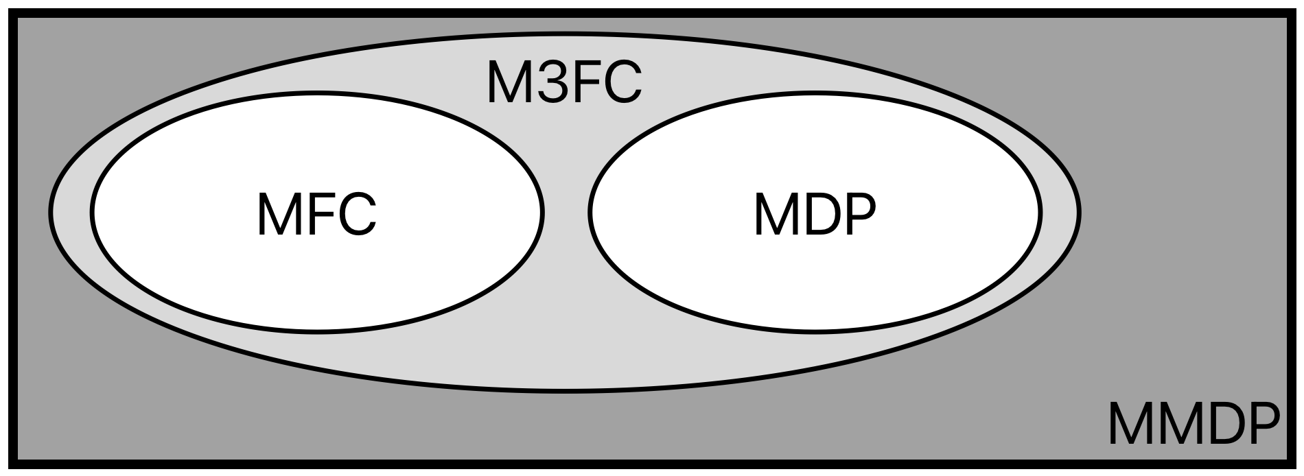
Figure 1: The proposed M3FC framework generalizes both MFC and MDPs in the space of general multi-agent MDPs (MMDPs).

Contributions.

In order to deal with the aforementioned gap between modelling strength and tractability, we formulate a general MFC-based MARL algorithm. Our contributions may be summarized as follows: (i) We formulate for the first time discrete-time major-minor MFC (M3FC), resulting in an extensive framework that generalizes MDPs and MFC while retaining desirable tractability properties in multi-agent control; (ii) We provide novel proofs for approximation guarantees and dynamic programming principles (DPPs) of MFC and M3FC by restricting to appropriate convergence modes and working with two characterizations of weak convergence. We relax continuity assumptions, extend from finite to compact spaces, and most importantly allow general stochastic mean fields; (iii) We use our framework as the basis for a powerful and tractable MARL scheme, directly applicable to finite systems with many agents in contrast to prior work, and capable of leveraging advances in single-agent RL. The algorithmic contribution is finally verified on various novel examples, outperforming state-of-the-art MARL techniques on exemplary many-agent systems. To the best of our knowledge, a comparison to MARL has not been performed yet, and approximation guarantees have not been shown for discrete-time MFC with compact state and action spaces, or major agents.

Notation: In the following, $\mathcal{P}(\mathcal{X})$ shall denote the space of probability measures on compact metric spaces $\mathcal{X}$, endowed with the topology of weak convergence. Unless noted otherwise, we metrize $\mathcal{P}(\mathcal{X})$ with the $1$-Wasserstein distance $W_{1}(\mu,\nu)\coloneqq\sup_{\lVert f\rVert_{\mathrm{Lip}}\leq 1}\left|\int f\,\mathrm{d}(\mu-\nu)\right|$ over real-valued $f$ with minimal Lipschitz constant $\lVert f\rVert_{\mathrm{Lip}}\leq 1$ Villani (2009). By compactness, we have the uniformly equivalent (but not Lipschitz equivalent) metric $d_{\Sigma}(\mu,\mu^{\prime})\coloneqq\sum_{m=1}^{\infty}2^{-m}|\int f_{m}\,\mathrm{d}(\mu-\mu^{\prime})|$ for a sequence of continuous $f_{m}\colon\mathcal{X}\to[-1,1]$ (cf. Parthasarathy (2005), Theorem 6.6). Note also that continuity is equivalent to uniform continuity in compact spaces $\mathcal{X}$, including $\mathcal{P}(\mathcal{X})$ by Prokhorov’s theorem Billingsley (2013). Proofs are found in the Appendix.

2 Deterministic Mean Field Control

Before we consider the most general model, for expository purposes it is instructive to first consider deterministic MFC, where we also extend existing theoretical results. Here, our proof technique generalizes existing approximation properties and dynamic programming principles beyond finite spaces and Lipschitz continuity assumptions to compact spaces and simple continuity. Our proof later allows an extension to common noise, major states and beyond.

2.1 Finite-Agent Control

Consider systems consisting of $N$ agents $i\in[N]\coloneqq\{1,\ldots,N\}$ with compact metric state and action spaces $\mathcal{X}$, $\mathcal{U}$ and corresponding random states and actions $x^{i,N}_{t}$ and $u^{i,N}_{t}$ at times $t\in\mathbb{N}$, where the initial states $x^{i,N}_{0}\sim\mu_{0}$ are independently sampled from some initial distribution $\mu_{0}\in\mathcal{P}(\mathcal{X})$. Depending on the actions, the agent states evolve according to a Markov kernel $p$ such that $x^{i,N}_{t+1}\sim p(x^{i,N}_{t+1}\mid x^{i,N}_{t},u^{i,N}_{t},\mu^{N}_{t})$, i.e. the dynamics depend (i) on the agent’s states and actions, and (ii) the anonymous system state given by the $\mathcal{P}(\mathcal{X})$-valued empirical distribution of states $\mu^{N}_{t}\coloneqq\frac{1}{N}\sum_{i=1}^{N}\delta_{x^{i,N}_{t}}$ – the so-called empirical mean field. Accordingly, we consider (possibly time-variant) feedback policies $\pi$ shared across all agents, reacting to the local agent state and mean field, $u^{i,N}_{t}\sim\pi_{t}(u^{i,N}_{t}\mid x^{i,N}_{t},\mu^{N}_{t})$. Lastly, define the infinite-horizon discounted maximization objective $J(\pi)\coloneqq\mathbb{E}\left[\sum_{t=0}^{\infty}\gamma^{t}r(\mu^{N}_{t})\right]$ with discount factor $\gamma\in(0,1)$ and reward function $r\colon\mathcal{P}(\mathcal{X})\to\mathbb{R}$, to optimize over a class $\Pi\subseteq\mathcal{P}(\mathcal{U})^{\mathcal{X}\times\mathcal{P}(\mathcal{X})\times\mathbb{N}}$ of policies. Overall, for all $i\in[N]$ and $t\in\mathbb{N}$, we have the finite MFC system

$$u^{i,N}_{t} \sim\pi_{t}(u^{i,N}_{t}\mid x^{i,N}_{t},\mu_{t}^{N}),$$ (1a)

$$x^{i,N}_{t+1} \sim p(x^{i,N}_{t+1}\mid x^{i,N}_{t},u^{i,N}_{t},\mu_{t}^{N}),$$ (1b)

$$J^{N}(\pi) =\operatorname{\mathbb{E}}\left[\sum_{t=0}^{\infty}\gamma^{t}r(\mu^{N}_{t})\right].$$ (1c)

Remark 2.1.

This model is as expressive as in many prior works Mondal et al. (2022); Gu et al. (2019), including (i) action or joint state-action mean fields $\nu_{t}\in\mathcal{P}(\mathcal{X}\times\mathcal{U})$ Mondal et al. (2022), by splitting time steps into two and defining the new state space $\mathcal{X}\cup\mathcal{X}\times\mathcal{U}$, (ii) average rewards over agents and (iii) conditionally random rewards $r_{t}^{i}$ by their expectation $r(\mu^{N}_{t})\equiv\frac{1}{N}\sum_{i=1}^{N}\operatorname{\mathbb{E}}\left[r_{t}^{i}\;\middle\lvert\;x^{i,N}_{t},\mu^{N}_{t}\right]$. A finite horizon objective can be handled analogously, though the existence of optimal stationary policies is no longer given. Note that while agents are modelled homogeneously, heterogeneity can be integrated into the agent state space.

In the following, we obtain a large, more tractable subclass of cooperative multi-agent control problems, which may otherwise suffer from the curse of many agents (combinatorial joint state-action spaces, e.g. Zhang et al. (2021)).

2.2 Mean Field Control

For tractability, one introduces the mean field limit by formally taking $N\to\infty$, and then showing its rigorous foundation for many-agent systems. The intractable finite-agent control problem is replaced by a more tractable, higher-dimensional single-agent MDP – the MFC MDP Carmona et al. (2019); Gu et al. (2021). Under a shared policy $\pi$, one abstracts the agents into their probability law, i.e. the mean field $\mu_{t}\equiv\mathcal{L}(x^{i,N}_{t})\in\mathcal{P}(\mathcal{X})$, which replaces its empirical analogue $\mu^{N}_{t}$ via a law of large numbers (LLN). Thus, by definition $\mu_{t}$ should evolve deterministically according to

$$\mu_{t+1}=T(\mu_{t},\mu_{t}\otimes\pi_{t}(\mu_{t}))\\ =\iint p(\cdot\mid x,u,\mu_{t})\pi_{t}(\mathrm{d}u\mid x,\mu_{t})\mu_{t}(\mathrm{d}x),$$ (2)

as verified in Theorem 2.7, with $\pi_{t}(\mu_{t})\coloneqq\pi_{t}(\cdot\mid\cdot,\mu_{t})$, the measures $\mu_{t}\otimes\pi_{t}(\mu_{t})$ on the product space $\mathcal{X}\times\mathcal{U}$, and the MFC dynamics $T(\mu,\nu)\coloneqq\iint p(\cdot\mid x,u,\mu)\nu(\mathrm{d}x,\mathrm{d}u)$.

Therefore, the states of the deterministic MFC MDP should consist only of the mean field $\mu_{t}$. For compactness reasons, the policies in $\Pi$ may induce $\mathcal{H}(\mu)$ or closed subsets thereof, which for any $\mu\in\mathcal{P}(\mathcal{X})$ is the compact subset $\mathcal{H}(\mu)\subseteq\mathcal{P}(\mathcal{X}\times\mathcal{U})$ of joint state-action distributions with first marginal $\mu$ (see Appendix A.2). We identify the action $\mu_{t}\otimes\pi_{t}(\mu_{t})\equiv h_{t}\in\mathcal{H}(\mu_{t})$, obtaining the MFC MDP

$$h_{t} \sim\hat{\pi}_{t}(h_{t}\mid\mu_{t}),$$ (3a)

$$\mu_{t+1} =T(\mu_{t},h_{t}),$$ (3b)

$$J(\hat{\pi}) =\operatorname{\mathbb{E}}\left[\sum_{t=0}^{\infty}\gamma^{t}r(\mu_{t})\right]$$ (3c)

with deterministic dynamics $T$, for ”upper-level” MFC policies $\hat{\pi}\in\hat{\Pi}$ mapping randomly from mean field $\mu_{t}$ to its desired state-action distribution $h_{t}$. For deterministic $\hat{\pi}$, we write $\pi_{t}=\Phi(\hat{\pi}_{t})$ to injectively reobtain agent policies by disintegration Kallenberg et al. (2017) of $h_{t}=\hat{\pi}_{t}(\mu_{t})$ into $\mu_{t}\otimes\pi^{\prime}_{t}$ and using $\pi_{t}(\mu_{t})\equiv\pi^{\prime}_{t}$. Inversely, any $\pi\in\Pi$ is representable in the MFC MDP by choosing $\hat{\pi}=\Phi^{-1}(\pi)$ via $\hat{\pi}_{t}(\mu_{t})=\mu_{t}\otimes\pi_{t}(\mu_{t})$.

2.3 Theoretical Analysis

Preempting the following results, we may solve the hard finite-agent system (1) near-optimally by instead solving the MFC MDP, allowing direct application of single-agent RL to the MFC MDP with approximate optimality in large systems. Mild continuity assumptions are required.

Assumption 2.2.

The transition kernel $p$ is continuous.

Assumption 2.3.

The reward $r$ is continuous.

Assumption 2.4.

The considered class of policies $\Pi$ is equi-Lipschitz, i.e. there exists $L_{\Pi}>0$ such that for all $t$ and $\pi\in\Pi$, $\pi_{t}\in\mathcal{P}(\mathcal{U})^{\mathcal{X}\times\mathcal{P}(\mathcal{X})}$ is $L_{\Pi}$-Lipschitz.

We note that the Lipschitz condition is inconsequential and standard Pasztor et al. (2021); Mondal et al. (2022), as (i) we may usually parametrize policies in a Lipschitz manner; (ii) neural networks are Lipschitz continuous; and (iii) Lipschitz policies should allow approximating other policies. In particular, Assumption 2.2 holds true in studied-before finite spaces, if each transition matrix entry of $P$ is continuous in the $|\mathcal{X}|$-dimensional mean field vector on the simplex (but not necessarily Lipschitz as in Gu et al. (2021); Mondal et al. (2022), the conditions of which we relax). Our assumptions imply continuity of the MFC dynamics $T$.

Lemma 2.5.

Under Assumption 2.2, we have $T(\mu_{n},\nu_{n})\to T(\mu,\nu)$ whenever $(\mu_{n},\nu_{n})\to(\mu,\nu)$,

First, we invoke a powerful, accessible DPP Hernández-Lerma & Lasserre (2012) to possibly solve for and show existence of a deterministic, time-independent optimal policy using the value function $V^{*}$, i.e. the fixed point of the Bellman equation $V^{*}(\mu)=\max_{h\in\mathcal{H}(\mu)}r(\mu)+\gamma V^{*}(T(\mu,h))$.

Theorem 2.6.

Under Assumptions 2.2 and 2.3, there exists an optimal stationary, deterministic policy $\hat{\pi}$ for (3), with $\hat{\pi}(\mu)\in\operatorname*{arg\,max}_{h\in\mathcal{H}(\mu)}r(\mu)+\gamma V^{*}(T(\mu,h))$.

Our proof constitutes an alternate approach to the one taken in Carmona et al. (2019). We use established and well-developed MDP theory, and later generalize to the major-minor case. As a result, we may (i) solve MFC problems analytically through the DPP, or (ii) later computationally by using policy gradients with stationary policies for the MFC MDP with naturally continuous actions: Finite state-action spaces lead to continuous MFC MDP actions $\mathcal{H}(\mu)$, while continuous spaces yield infinite-dimensional $\mathcal{H}(\mu)$, motivating policy gradient methods.

Lastly, we show propagation of chaos Sznitman (1991), i.e. convergence of empirical distributions to the mean field, in order to obtain the approximate optimality of MFC solutions in the finite system, theoretically backing the reduction of finite-agent control to ”single-agent” MFC MDPs. Here, prior results Gu et al. (2021); Mondal et al. (2022) are extended to quite general compact spaces.

Theorem 2.7.

Fix any family of equicontinuous functions $\mathcal{F}\subseteq\mathbb{R}^{\mathcal{P}(\mathcal{X})}$. Under Assumption 2.2 and 2.4, the empirical mean field converges weakly, uniformly over $f\in\mathcal{F}$, $\pi\in\Pi$, $\Phi^{-1}(\pi)\in\hat{\Pi}$, to the limiting mean field at all times $t\in\mathbb{N}$,

$$\sup_{\pi\in\Pi}\sup_{f\in\mathcal{F}}\left|\operatorname{\mathbb{E}}\left[f(\mu^{N}_{t})\right]-\operatorname{\mathbb{E}}\left[f(\mu_{t})\right]\right|\to 0.$$ (4)

Therefore, we may solve the difficult finite control problem by detouring over the corresponding MFC MDP, which we solve using powerful single-agent RL techniques in Section 4. See also Figure 2 for the corresponding diagram.

Figure 2: Approximation of multi-agent control by MFC (blue path). Otherwise intractable $N$-agent control problems are first abstracted into MFC, the solution of which then constitutes an approximately optimal solution in the $N$-agent control problem.

Corollary 2.8.

Under Assumptions 2.2, 2.3 and 2.4, an optimal deterministic policy in the MFC $\pi^{*}\in\operatorname*{arg\,max}_{\hat{\pi}}J(\hat{\pi})$ with $\Phi(\pi^{*})\in\Pi$ results in an $\varepsilon$-optimal policy $\Phi(\pi^{*})$ in the finite-agent system with $\varepsilon\to 0$ as $N\to\infty$,

$$J^{N}(\Phi(\pi^{*}))\geq\sup_{\pi\in\Pi}J^{N}(\pi)-\varepsilon.$$ (5)

3 Stochastic Mean Field Control

In this section, we extend MFC by allowing for stochastic mean fields and a major agent that is not abstractable into its distribution. Overall, we obtain a tractable class of models that generalizes both MDPs and classical MFC. We will use the same symbols as in Section 2, extended accordingly.

3.1 Common Noise and Major States

In the classical sense Perrin et al. (2020); Motte & Pham (2022a), common noise is given by random noise $\epsilon^{0}_{t}\sim p_{\epsilon}(\epsilon^{0}_{t})$ sampled from a stationary distribution $p_{\epsilon}$ and affecting all minor agents at once, $x^{i,N}_{t+1}\sim p(x^{i,N}_{t+1}\mid x^{i,N}_{t},u^{i,N}_{t},\epsilon^{0}_{t},\mu_{t}^{N})$. This allows describing systems with stochastic mean fields and inter-agent correlation, and has added difficulty to the theoretical analysis Carmona et al. (2016).

We go beyond common noise by general major states $x^{0,N}_{t}$ indexed by agent index $i=0$, which need not be sampled from fixed distributions but may evolve dynamically. Consider major states $x^{0,N}_{t}$ from a compact major state space $\mathcal{X}^{0}$ in addition to the prequel. The major state is sampled from an initial distribution $\mu^{0}_{0}\in\mathcal{P}(\mathcal{X}^{0})$ and evolves according to a transition kernel $p^{0}$ as $x^{0,N}_{t+1}\sim p^{0}(x^{0,N}_{t+1}\mid x^{0,N}_{t},\mu_{t}^{N})$. Letting the major state influence minor agents gives the novel system with major states (22) in Appendix B, with corresponding limiting system and results analogous to the following more general model with major agents.

3.2 Major-Minor MFC

In a final step, we generalize both MFC and MDPs to deal with both minor and major agents. As a result, our novel model tractably describes many-agent systems with both MFC and MDP components. Note that the major agent state may include also any components of the environment unrelated to agents, e.g. cars in a routing problem affected by construction sites, controlled traffic lights and other dynamical circumstances that are not bound to a specific car.

We consider major actions $u^{0,N}_{t}$ in a compact major action space $\mathcal{U}^{0}$, sampled from policies $\pi^{0}\in\Pi^{0}$ in the space of major agent policies $\Pi^{0}\subseteq\mathcal{P}(\mathcal{U}^{0})^{\mathcal{X}^{0}\times\mathcal{P}(\mathcal{X})\times\mathbb{N}}$. Allowing major actions to affect dynamics and rewards, we formulate the finite M3FC system

$$u^{i,N}_{t} \sim\pi_{t}(u^{i,N}_{t}\mid x^{i,N}_{t},x^{0,N}_{t},\mu_{t}^{N}),$$ (6a)

$$x^{i,N}_{t+1} \sim p(x^{i,N}_{t+1}\mid x^{i,N}_{t},u^{i,N}_{t},x^{0,N}_{t},u^{0,N}_{t},\mu_{t}^{N}),$$ (6b)

$$u^{0,N}_{t} \sim\pi^{0}_{t}(u^{0,N}_{t}\mid x^{0,N}_{t},\mu_{t}^{N}),$$ (6c)

$$x^{0,N}_{t+1} \sim p^{0}(x^{0,N}_{t+1}\mid x^{0,N}_{t},u^{0,N}_{t},\mu_{t}^{N}),$$ (6d)

$$J^{N}(\pi,\pi^{0}) =\operatorname{\mathbb{E}}\left[\sum_{t=0}^{\infty}\gamma^{t}r(x^{0,N}_{t},u^{0,N}_{t},\mu^{N}_{t})\right],$$ (6e)

and accordingly the limiting M3FC MDP

$$h_{t} \sim\hat{\pi}(h_{t}\mid x^{0}_{t},\mu_{t}),$$ (7a)

$$\mu_{t+1} =T(x^{0}_{t},u^{0}_{t},\mu_{t},h_{t}),$$ (7b)

$$u^{0}_{t} \sim\pi^{0}(u^{0}_{t}\mid x^{0}_{t},\mu_{t}),$$ (7c)

$$x^{0}_{t+1} \sim p^{0}(x^{0}_{t+1}\mid x^{0}_{t},u^{0}_{t},\mu_{t}),$$ (7d)

$$J(\hat{\pi},\pi^{0}) =\operatorname{\mathbb{E}}\left[\sum_{t=0}^{\infty}\gamma^{t}r(x^{0}_{t},u^{0}_{t},\mu_{t})\right]$$ (7e)

with $T(x^{0},u^{0},\mu,h)\coloneqq\iint p(\cdot\mid x,u,x^{0},u^{0},\mu)h(\mathrm{d}x,\mathrm{d}u)$, where we identify $(h_{t},u^{0}_{t})$ as the action of the M3FC MDP, and $(x^{0}_{t},\mu_{t})$ as its state, visualized also in Figure 3.

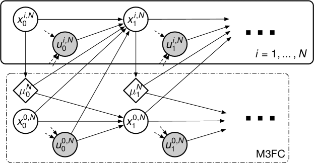
Figure 3: The dynamics model as a probabilistic graphical model, with actions in grey (inputs omitted for readability). The diamond denotes a deterministic function of its inputs. The M3FC approach hides minor agents $i\in[N]$ by a LLN, considering only their distribution, i.e. the variables in the dotted box.

As shown in Figure 1, the M3FC generalizes both MDP and MFC in the space of multi-agent Markov decision processes (MMDP, e.g. Oliehoek & Amato (2016)). In other words, M3FC handles both highly general single agents and many minor agents at the same time. Here, we understand MFC and M3FC as frameworks for multi-agent control, and not e.g. the limiting M3FC MDP, which is – formally – an MDP.

Remark 3.1.

Strictly speaking, in centralized MMDPs one may select jointly $(u^{0,N}_{t},u^{1,N}_{t},\ldots,u^{N,N}_{t})$ given joint states $(x^{0,N}_{t},x^{1,N}_{t},\ldots,x^{N,N}_{t})$. However, under mean field dynamics, by the LLN (i) information from the joint state should reduce to $(x^{0,N}_{t},\mu^{N}_{t})$, while (ii) joint actions would be replaced by LLN via sampling from $h_{t}$. We conjecture that it is possible to extend optimality (e.g. Corollary 3.8) over larger such classes of policies, see Appendix C.

3.3 Theoretical Analysis

We now perform a theoretical analysis of the novel M3FC model. For the proof, we now assume Lipschitz continuity.

Assumption 3.2.

The transition kernels $p$, $p^{0}$ are Lipschitz continuous with constants $L_{p}$, $L_{p^{0}}$.

Assumption 3.3.

The reward $r$ is Lipschitz continuous.

Assumption 3.4.

The classes of policies $\Pi$, $\Pi^{0}$ are equi-Lipschitz, i.e. there exist $L_{\Pi},L_{\Pi^{0}}$ as in Assumption 2.4.

As in deterministic MFC, we obtain a DPP by defining again the value function via the Bellman equation $V^{*}(x^{0},\mu)=\max_{(h,u^{0})\in\mathcal{H}(\mu)\times\mathcal{U}^{0}}r(x^{0},u^{0},\mu)+\gamma\mathbb{E}_{y^{0}\sim p^{0}(y^{0}\mid x^{0},u^{0},\mu)}V^{*}(y^{0},T(x^{0},u^{0},\mu,h))$.

Theorem 3.5.

Under Assumptions 3.2 and 3.3, there exist optimal stationary, deterministic policies $\hat{\pi}$, $\pi^{0}$ for the M3FC MDP (7) by choosing $(\hat{\pi}(x^{0},\mu),\pi^{0}(x^{0},\mu))$ from the maximizers of $\operatorname*{arg\,max}_{(h,u^{0})\in\mathcal{H}(\mu)\times\mathcal{U}^{0}}r(x^{0},u^{0},\mu)+\gamma\mathbb{E}_{y^{0}\sim p^{0}(y^{0}\mid x^{0},u^{0},\mu)}V^{*}(y^{0},T(x^{0},u^{0},\mu,h))$.

Remark 3.6.

Note that though (7) has independent $\hat{\pi}$ and $\pi^{0}$, we still obtain existence of optimal deterministic stationary $\hat{\pi}$, $\pi^{0}$ via existence of such M3FC policies $\tilde{\pi}\equiv\hat{\pi}\otimes\pi^{0}$, $(h_{t},u^{0}_{t})\sim\tilde{\pi}((h_{t},u^{0}_{t})\mid x^{0}_{t},\mu_{t})$ by Theorem 3.5.

Hence again, as in the MFC case, we may solve analytically via the DPP or use policy gradients with stationary policies, motivating the M3FC model together with the following convergence results and approximate optimality of M3FC MDP solutions in the finite M3FC system.

Theorem 3.7.

Fix any family of equi-Lipschitz functions $\mathcal{F}\subseteq\mathbb{R}^{\mathcal{X}^{0}\times\mathcal{U}^{0}\times\mathcal{P}(\mathcal{X})}$ with shared Lipschitz constant $L_{\mathcal{F}}$ for all $f\in\mathcal{F}$. Under Assumptions 3.2 and 3.4, the random variable $(x^{0,N}_{t},u^{0,N}_{t},\mu_{t}^{N})$ converges weakly, uniformly over $f\in\mathcal{F}$, $\pi\in\Pi$, $\pi^{0}\in\Pi^{0}$, to $(x^{0}_{t},u^{0}_{t},\mu_{t})$ at all times $t\in\mathbb{N}$,

$$\sup_{f,\pi,\pi^{0}}\left|\operatorname{\mathbb{E}}\left[f(x^{0,N}_{t},u^{0,N}_{t},\mu_{t}^{N})-f(x^{0}_{t},u^{0}_{t},\mu_{t})\right]\right|\to 0.$$ (8)

The result is a more tractable framework for general systems of many agents by conceptually reducing to higher-dimensional MDPs, which will provide us a basis for MARL algorithms with the following $\varepsilon$-optimality guarantee.

Corollary 3.8.

Under Assumptions 3.2, 3.3 and 3.4, optimal deterministic policies $(\pi^{*},\pi^{0*})\in\operatorname*{arg\,max}_{(\hat{\pi},\pi^{0})}J(\hat{\pi},\pi^{0})$ in the M3FC MDP with $\Phi(\pi^{*})$ yield $\varepsilon$-optimal $(\Phi(\pi^{*}),\pi^{0*})$ in the finite M3FC system with $\varepsilon\to 0$ as $N\to\infty$,

$$J^{N}(\Phi(\pi^{*}),\pi^{0*})\geq\sup_{(\pi,\pi^{0})\in\Pi\times\Pi^{0}}J^{N}(\pi,\pi^{0})-\varepsilon.$$ (9)

4 Major-Minor Mean Field MARL

In order to solve multi-agent control, it is crucial to find tractable sample-based MARL techniques, both for (i) otherwise too complex problems and (ii) for problems where we have no access to the dynamics or reward model. On the one hand, RL has been applied to solve MFC. On the other, we could use the MFC formalism to instead give rise to novel MARL algorithms. While literature often focuses on the former Carmona et al. (2019); Pasztor et al. (2021); Mondal et al. (2022), in our work we understand the proposed algorithm as both a solution to M3FC MDPs, and to the more interesting, actual finite system. We apply the following perspective: By Theorem 3.7, the MFC MDP is approximated well by the finite system. Therefore, there is no need to solve the limiting M3FC MDP, and instead it is sufficient to apply our proposed MFC solution directly to finite MFC systems. In particular, accessing an MFC MDP would already allow instantiating finite systems of any size.

Algorithm 1 Major-Minor Mean Field PPO (M3FPPO)

1:  Initialize PPO policy $\pi^{\theta}_{\mathrm{RL}}$ and value critic $V^{\psi}$.

2:  for iterations $n=0,1,\ldots$ do

3:     Initialize empty batch buffer $B=\emptyset$.

4:     for time step $t=0,\ldots,B_{\mathrm{len}}-1$ do

5:        Sample M3FC MDP action from PPO policy, $u_{t}\equiv(u^{0,N}_{t},\pi^{\prime}_{t})\sim\pi^{\theta}_{\mathrm{RL}}((u^{0,N}_{t},\pi^{\prime}_{t})\mid x^{0,N}_{t},\mu^{N}_{t})$.

6:        for minor agent $i=1,\ldots,N$ do

7:           Sample actions $u^{i,N}_{t}\sim\pi^{\prime}_{t}(u^{i,N}_{t}\mid x^{i,N}_{t})$.

8:        end for

9:        Execute actions $\{u^{i,N}_{t}\}_{i=0,1,\ldots}$ in environment.

10:        Observe reward $r^{N}_{t}$, next states $\{x^{i,N}_{t+1}\}_{i=0,1,\ldots}$, and episode termination flag $d_{t+1}\in\{0,1\}$.

11:        Add $((x^{0,N}_{t},\mu^{N}_{t}),u_{t},r^{N}_{t},d_{t+1},(x^{0,N}_{t+1},\mu^{N}_{t+1}))$ (a transition sample) to batch buffer $B$.

12:     end for

13:     Compute GAE advantages $\hat{A}$ on $B$.

14:     for update epoch $i=1,\ldots,N_{\mathrm{SGD}}$ do

15:        Sample mini-batch $b$ randomly from $B$.

16:        Update $\theta$ via PPO loss gradient $\nabla_{\theta}L_{\theta}$ on data $b$.

17:        Update $\psi$ via $L_{2}$ loss gradient $\nabla_{\psi}L_{\psi}$ on data $b$.

18:     end for

19:  end for

MDP-based MARL.

Since we know by Theorem 3.5 that there exists an optimal stationary policy, we solve the M3FC MDP (7) using standard stationary policies and single-agent RL, aptly referred to as major-minor mean field MARL (M3FMARL). Here, the M3FC MDP (7) is actually given by a large MARL problem (6), i.e. in a sense the natural particle filter approximation for the M3FC MDP. Specifically, we will use the proximal policy optimization (PPO) algorithm Schulman et al. (2017) to obtain a M3FC policy $\pi_{\mathrm{RL}}$ according to Algorithm 1, but other RL algorithms could also be used. Beyond improved tractability, an advantage of this approach is therefore that we can profit from any advances in single-agent RL. For this purpose, we must first provide a parametric form of the mean fields in $\mathcal{P}(\mathcal{X})$ and the joint distribution part of M3FC MDP actions $\mathcal{H}(\mu^{N}_{t})$.

Parametrization of spaces.

For discrete $\mathcal{X}$, $\mathcal{U}$, this is straightforward by finite-dimensional vectors $\mu^{N}_{t}\in\mathcal{P}(\mathcal{X})$ on the simplex and by considering as part of the M3FC policy actions the two-dimensional matrix $O\in[-1,1]^{\mathcal{X}\times\mathcal{U}}$. The values of $O$ are then mapped to probabilities of actions in any state $\pi^{\prime}_{t}(u\mid x)=\frac{O_{xu}+1+\epsilon}{\sum_{u^{\prime}\in\mathcal{U}}(O_{xu^{\prime}}+1+\epsilon)}$ for a small $\epsilon=10^{-10}$ for numerical stability. The implicitly defined M3FC MDP action $h^{N}_{t}\in\mathcal{H}(\mu^{N}_{t})$ is hence $h^{N}_{t}\equiv\mu^{N}_{t}\otimes\pi^{\prime}_{t}(u\mid x)$, where $O\sim\pi_{\mathrm{RL}}(O\mid x^{0,N}_{t},\mu^{N}_{t})$ is sampled from RL policy $\pi_{\mathrm{RL}}$. For continuous $\mathcal{X}$, $\mathcal{U}$, we partition $\mathcal{X}$ into $M$ bins and represent $\mu^{N}_{t}$ by binned histograms. Action distributions are instead parametrized by affinely mapping values $O\in[-1,1]^{M\times 2}$ to (clipped) diagonal Gaussian parameters, e.g. $\mu_{\mathcal{X}_{i}}\in\mathcal{U}$, $\sigma_{\mathcal{X}_{i}}\in[\epsilon,0.25+\epsilon]$ of $\mathcal{N}(\mu_{\mathcal{X}_{i}},\sigma_{\mathcal{X}_{i}})\in\mathcal{P}(\mathcal{U})$ defined for all $M$ equisized bins $\mathcal{X}_{i}\subseteq\mathcal{X}$, constituting $\pi^{\prime}_{t}$.

Hierarchical structure.

The M3FC MDP state $(x^{0,N}_{t},\mu^{N}_{t})$ is fed into the policy, while the distribution of major actions $u^{0,N}_{t}$ is parametrized via categorical or diagonal Gaussian distributions for discrete and continuous $\mathcal{U}^{0}$ respectively. Sampling major actions and $O$ from $\pi_{\mathrm{RL}}$, and minor actions from $\pi^{\prime}_{t}$, allows direct application of PPO to MARL (6) and completes M3FPPO by observing next states $(x^{0,N}_{t+1},\mu^{N}_{t+1})$ and reward $r^{N}_{t}$, see also Algorithm 1. Overall, Algorithm 1 is ”hierarchical” in that M3FC MDP actions specify behavior at once for all minor agents.

Centralized training, decentralized execution.

Our algorithm falls into the centralized training decentralized execution (CTDE) paradigm Zhang et al. (2021), as we sample a single central M3FC MDP action during training, but enable decentralized execution by sampling $\pi^{\prime}_{t}$ instead separately on each agent (before line $7$ in Algorithm 1). For instance assuming a deterministic M3FC policy (of which an optimal one is guaranteed to exist by Theorem 3.5), the M3FC action will trivially be equal for all agents. Regardless, we also verify decentralized execution experimentally.

Comparison.

We compare against independent PPO (IPPO), i.e. PPO with independent learning Tan (1993) and parameter sharing Gupta et al. (2017), which often shows state-of-the-art performance in cooperative MARL de Witt et al. (2020); Papoudakis et al. (2021); Yu et al. (2022), though we separate major and minor agent policies for performance. To compare, we use the same observations (where minor agents additionally observe own states), policy architecture, PPO implementation and hyperparameters as in M3FPPO.

5 Experiments

In this section, we demonstrate the applicability of M3FPPO on illustrative problems. We use $M=49$ bins ($M=7$ in Potential) and train M3FPPO on the natural approximation of the M3FC system, which is the finite-agent system (6) with $N=300$ agents (training for lower $N$ in Appendix D). For implementation and problem details, see Appendix D.

5.1 Problems

The 2G problem is a simple major state problem, where minor agents should form a sinusoidal time-variant mixture of two Gaussians $\mu^{*}_{t}$ – the major state – which is noisily observed analogously to $\mu^{N}_{t}$ by binning into $M=49$ bins.

In the Formation problem, the added major agent should stay close to an Ornstein-Uhlenbeck target, while minor agents should form a Gaussian around the major agent.

The Beach Bar process is an adapted classic Perrin et al. (2020), where minor agents minimize their distance to a bar, and crowdedness. Here, we consider a discrete torus variant, with a moving bar following a randomly walking target.

In the Foraging problem, agents must forage from random foraging areas, e.g. consider a movement-limited package truck with minor drones picking up packages in a city. The minor agents gain encumbrance proportional to closeness to foraging area, and empty their load at the major agent.

Lastly, in the Potential problem, minor agents move to generate a potential landscape on a continuous one-dimensional torus (sphere), the gradient of which is followed by the major agent to keep it close to an Ornstein-Uhlenbeck target.

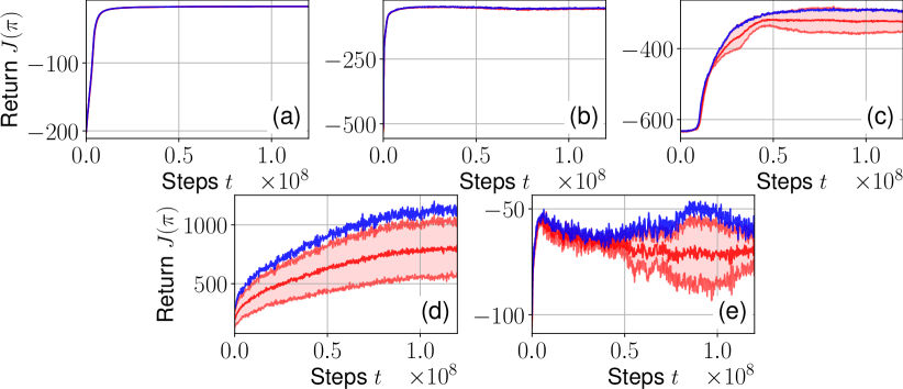
Figure 4: Training curves (mean episode return) of M3FPPO (red), with standard deviation (three trials, shaded) and maximum (blue). (a) 2G; (b) Formation; (c) Beach Bar; (d) Foraging; (e) Potential.

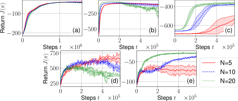
Figure 5: Training curves of IPPO, as in Figure 4 (no maxima).

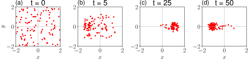
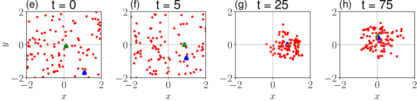
Figure 6: Qualitative visualization of learned MFC behavior in the simple 2G (a-d) and Formation (e-h) problems. Red: minor agent; blue triangle: major agent; green triangle: major agent target.

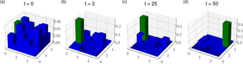
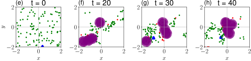
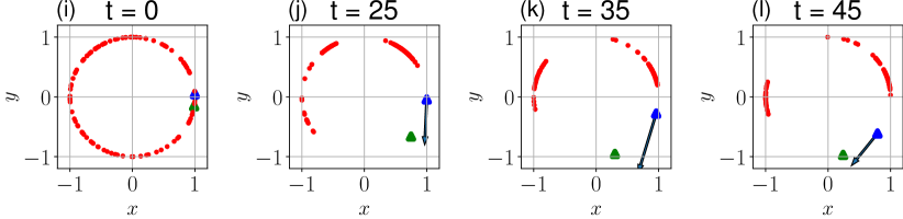
Figure 7: Qualitative visualization of learned MFC behavior in the Beach (a-d), Foraging (e-h) and Potential (i-l) problems. (a-d): empirical distribution of states, with major agent and target both in green; (e-h): As in Figure 6(e-h), but green for less-than-half-encumbered minor agents, and red otherwise; Foraging areas are indicated in purple; (i-l): As in Figure 6(e-h), with arrow indicating the current potential gradient (not to scale).

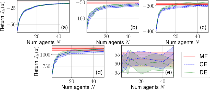
Figure 8: The mean episode return of the final learned MFC policy in finite $N$-agent systems over (a-c) $100$, (d) $300$ or (e) $500$ trials, with 95% confidence interval (shaded). MF: CE for $N=500$; CE: centralized execution; DE: decentralized execution.

5.2 Training results

In Figure 4 and Appendix D, we see that M3FPPO stably obtains good results, despite the fact that a MARL problem is solved, as M3FPPO reduces otherwise hard many-agent problems to single-agent RL of higher dimension. Though RL nonetheless remains difficult and could profit from intricate hyperparameter tuning, M3FPPO trains comparatively stably by avoiding various pathologies of MARL techniques such as non-stationarity of multi-agent learning, or the exponential nature of joint state-actions Zhang et al. (2021). On the other hand, IPPO under the same hyperparameters leads to the sometimes unstable training seen in Figure 5. This is intuitive, as for many agents, the reward signal for any single agent’s action can sometimes become uninformative (as a cooperative ”averaged” signal over all agents).

Qualitative behavior.

In Figure 6, it can be seen that M3FPPO successfully learns to form mixtures of Gaussians in 2G, and a Gaussian around a moving major agent successfully tracking its target in Formation. As expected in 2G, the two Gaussians at their sinusoidal peaks $t=25$ and $t=50$ are not perfectly tracked, in order to minimize the cost in following time steps, when the other Gaussian reappears. Meanwhile, in Figure 7 we observe success in Beach, Foraging and Potential: In Beach, M3FPPO learns to accumulate up to $70\%$ of agents on the bar, as more will lead to a decrease in reward. In Foraging, agents successfully deplete the foraging areas in the bottom left after moving on to other areas. Lastly, in Potential, the minor agents usually successfully push the major agent towards its current target.

Finite system and decentralized execution.

In Figure 8, we transfer the trained M3FPPO policy to $N=2,\ldots,50$, comparing against the performance in the limiting system (with $N=500$). We observe that as $N$ grows, the performance converges to that of the limiting system, supporting Theorem 3.7 and Corollary 3.8. We thus conclude transferability to varying numbers of agents. In an ablation in Appendix D, we alternatively also find similar success in directly training M3FPPO on small $N$-agent systems instead of transferring behavior from a large limiting system.

Comparing Figures 4, 5 and 8, we see that (i) by experience sharing, IPPO can be more sample efficient, partly as time steps give $N$ samples instead of just one in M3FPPO; (ii) however, except in Potential, M3FPPO outperforms or matches IPPO for many agents, even if IPPO stops early at its maximum during training (comparing best of $3$ trials at $N=20$, in 2G $-23$ vs. $-42$, Beach $-310$ vs. $-350$, Formation both $-60$, and especially Foraging $1000$ vs. $570$).

Lastly, we verify the effect of fully decentralized execution by agent-wise randomization, i.e. instead of sampling a single centralized M3FC action, we apply the upper-level policy on each agent separately. It turns out that decentralized execution has little effect and can even marginally improve performance, e.g. in Beach, see Figure 8.

6 Discussion

We have proposed a generalization of MDPs and MFC, enabling tractable MARL on quite general many-agent systems, with both theoretical and empirical support. For future work, one could attempt to show extended optimality results as discussed in Appendix C, consider more refined approximations Gast & Van Houdt (2018), local Qu et al. (2020b) and global interactions together, or apply the framework in practice. Algorithmically, parametrization of M3FC MDP actions $\mathcal{H}(\mu)$ could move beyond binning of $\mathcal{X}$ to further gain performance, e.g. via kernel methods. Hyperparameter tuning could additionally improve results. Lastly, another goal is quantifying convergence to the classical rate $\mathcal{O}(1/\sqrt{N})$ Huang et al. (2006), as the current proof would require difficult-to-verify $d_{\Sigma}$-Lipschitz assumptions.

Appendix A Proofs

Here, we provide lengthy proofs that were omitted in the main text.

A.1 Proof of Lemma 2.5

Proof.

To show $T(\mu_{n},\nu_{n})\to T(\mu,\nu)$, consider any Lipschitz and bounded $f$ with Lipschitz constant $L_{f}$, then

$$\left|\int f\,\mathrm{d}(T(\mu_{n},\nu_{n})-T(\mu,\nu))\right|$$

$$=\left|\iiint f(x^{\prime})p(\mathrm{d}x^{\prime}\mid x,u,\mu_{n})\nu_{n}(\mathrm{d}x,\mathrm{d}u)-\iiint f(x^{\prime})p(\mathrm{d}x^{\prime}\mid x,u,\mu)\nu(\mathrm{d}x,\mathrm{d}u)\right|$$

$$\quad\leq\iint\left|\int f(x^{\prime})p(\mathrm{d}x^{\prime}\mid x,u,\mu_{n})-\int f(x^{\prime})p(\mathrm{d}x^{\prime}\mid x,u,\mu)\right|\nu_{n}(\mathrm{d}x,\mathrm{d}u)$$

$$\qquad+\left|\iiint f(x^{\prime})p(\mathrm{d}x^{\prime}\mid x,u,\mu)(\nu_{n}(\mathrm{d}x,\mathrm{d}u)-\nu(\mathrm{d}x,\mathrm{d}u))\right|$$

$$\quad\leq\sup_{x\in\mathcal{X},u\in\mathcal{U}}L_{f}W_{1}(p(\cdot\mid x,u,\mu_{n}),p(\cdot\mid x,u,\mu))$$

$$\qquad+\left|\iiint f(x^{\prime})p(\mathrm{d}x^{\prime}\mid x,u,\mu)(\nu_{n}(\mathrm{d}x,\mathrm{d}u)-\nu(\mathrm{d}x,\mathrm{d}u))\right|\to 0$$

for the first term by $1$-Lipschitzness of $\frac{f}{L_{f}}$ and Assumption 2.2 (with compactness implying the uniform continuity), and for the second by $\nu_{n}\to\nu$ and from continuity by the same argument of $(x,u)\mapsto\iint f(x^{\prime})p(\mathrm{d}x^{\prime}\mid x,u,\mu)$. ∎

A.2 Proof of Theorem 2.6

Proof.

The MFC MDP fulfills Hernández-Lerma & Lasserre (2012), Assumption 4.2.1. Here, we use Hernández-Lerma & Lasserre (2012), Condition 3.3.4(b1) instead of (b2), see also alternatively Hernández-Lerma & Muñoz de Ozak (1992).

More specifically, for Hernández-Lerma & Lasserre (2012), Assumption 4.2.1(a), the cost function $-r$ is continuous by Assumption 2.3, therefore also bounded by compactness of $\mathcal{P}(\mathcal{X})$, and finally also inf-compact on the state-action space of the MFC MDP, since for any $\mu\in\mathcal{P}(\mathcal{X})$ the set $\{h\in\mathcal{H}(\mu)\mid-r(\mu)\leq c\}$ is trivially given by $\mathcal{H}(\mu)$ whenever $-r(\mu)\leq c$, or $\emptyset$ otherwise. Here, we show that $\mathcal{H}(\mu)\subseteq\mathcal{P}(\mathcal{X}\times\mathcal{U})$ is a subset of the compact space $\mathcal{P}(\mathcal{X}\times\mathcal{U})$ that is closed (and therefore also compact). Note first that two measures $\mu,\mu^{\prime}\in\mathcal{P}(\mathcal{X})$ are equal if and only if for all continuous and bounded $f$ we have $\int f\,\mathrm{d}\mu=\int f\,\mathrm{d}\mu^{\prime}$, see e.g. Billingsley (2013), Theorem 1.3.

Therefore, as $\mathcal{H}(\mu)$ is defined by its first marginal $\mu$, $\mathcal{H}(\mu)$ can be written as an intersection

$$\mathcal{H}(\mu)=\bigcap_{f\in C_{b}(\mathcal{X})}\left\{h\in\mathcal{P}(\mathcal{X}\times\mathcal{U})\;\middle\lvert\;\int f\otimes\mathbf{1}\,\mathrm{d}h=\int f\,\mathrm{d}\mu\right\}$$

of closed sets: Since $h\mapsto\int f\otimes\mathbf{1}\,\mathrm{d}h$ is continuous, its preimage of the closed set $\{\int f\,\mathrm{d}\mu\}$ is closed. Here, $\otimes$ denotes the tensor product of $f$ with the function $\mathbf{1}$ equal one, i.e. $f\otimes\mathbf{1}$ is the map $(x,u)\mapsto f(x)$.

Similarly, for Hernández-Lerma & Lasserre (2012), Assumption 4.2.1(b), the transition dynamics $T$ are weakly continuous, as for any $(\mu_{n},\nu_{n})\to(\mu,\nu)\in\mathcal{P}(\mathcal{X})\times\mathcal{P}(\mathcal{X}\times\mathcal{U})$ we have $T(\mu_{n},\nu_{n})\to T(\mu,\nu)$ by Lemma 2.5 and therefore $\int f\,\mathrm{d}\delta_{T(\mu_{n},\nu_{n})}=f(T(\mu_{n},\nu_{n}))\to f(T(\mu,\nu))=\int f\,\mathrm{d}\delta_{T(\mu,\nu)}$ for any continuous and bounded $f\colon\mathcal{P}(\mathcal{X})\to\mathbb{R}$.

Furthermore, the MFC MDP fulfills Hernández-Lerma & Lasserre (2012), Assumption 4.2.2 by boundedness of $r$ from Assumption 2.3. Therefore, the desired statement follows from Hernández-Lerma & Lasserre (2012), Theorem 4.2.3. ∎

A.3 Proof of Theorem 2.7

Proof.

The statement (4) is shown inductively over $t\geq 0$. At time $t=0$, (4) holds by the weak LLN argument, see also the first term below. Assuming (4) at time $t$, then for time $t+1$ we have

$$\sup_{\pi\in\Pi}\sup_{f\in\mathcal{F}}\left|\operatorname{\mathbb{E}}\left[f(\mu^{N}_{t+1})-f(\mu_{t+1})\right]\right|$$

$$\quad\leq\sup_{\pi\in\Pi}\sup_{f\in\mathcal{F}}\left|\operatorname{\mathbb{E}}\left[f(\mu^{N}_{t+1})-f(T(\mu^{N}_{t},\mu^{N}_{t}\otimes\pi_{t}(\mu^{N}_{t})))\right]\right|$$ (10)

$$\qquad+\sup_{\pi\in\Pi}\sup_{f\in\mathcal{F}}\left|\operatorname{\mathbb{E}}\left[f(T(\mu^{N}_{t},\mu^{N}_{t}\otimes\pi_{t}(\mu^{N}_{t})))-f(\mu_{t+1})\right]\right|.$$ (11)

For the first term (10), first note that by compactness of $\mathcal{P}(\mathcal{X})$, $\mathcal{F}$ is uniformly equicontinuous, and hence admits a non-decreasing, concave (as in DeVore & Lorentz (1993), Lemma 6.1) modulus of continuity $\omega_{\mathcal{F}}\colon[0,\infty)\to[0,\infty)$ where $\omega_{\mathcal{F}}(x)\to 0$ as $x\to 0$ and $|f(\mu)-f(\nu)|\leq\omega_{\mathcal{F}}(W_{1}(\mu,\nu))$ for all $f\in\mathcal{F}$.

We also have uniform equicontinuity of $\mathcal{F}$ with respect to the space $(\mathcal{P}(\mathcal{X}),d_{\Sigma})$ instead of $(\mathcal{P}(\mathcal{X}),W_{1})$, as the identity map $\mathrm{id}\colon(\mathcal{P}(\mathcal{X}),d_{\Sigma})\to(\mathcal{P}(\mathcal{X}),W_{1})$ is uniformly continuous (as both $d_{\Sigma}$ and $W_{1}$ metrize the topology of weak convergence, and $\mathcal{P}(\mathcal{X})$ is compact), and therefore there exists a modulus of continuity $\tilde{\omega}$ for the identity map such that for any $\mu,\nu\in(\mathcal{P}(\mathcal{X}),d_{\Sigma})$, by the prequel

$$|f(\mu)-f(\nu)|\leq\omega_{\mathcal{F}}(W_{1}(\mathrm{id}\,\mu,\mathrm{id}\,\nu))\leq\omega_{\mathcal{F}}(\tilde{\omega}(d_{\Sigma}(\mu,\nu)))$$

with $\tilde{\omega}_{\mathcal{F}}\coloneqq\omega_{\mathcal{F}}\circ\tilde{\omega}$, which can be replaced by its least concave majorant (again as in DeVore & Lorentz (1993), Lemma 6.1).

Therefore, by Jensen’s inequality, for (10) we obtain

$$\left|\operatorname{\mathbb{E}}\left[f(\mu^{N}_{t+1})-f(T(\mu^{N}_{t},\mu^{N}_{t}\otimes\pi_{t}(\mu^{N}_{t})))\right]\right|$$

$$\quad\leq\operatorname{\mathbb{E}}\left[\tilde{\omega}_{\mathcal{F}}(d_{\Sigma}(\mu^{N}_{t+1},T(\mu^{N}_{t},\mu^{N}_{t}\otimes\pi_{t}(\mu^{N}_{t}))))\right]$$

$$\quad\leq\tilde{\omega}_{\mathcal{F}}\left(\operatorname{\mathbb{E}}\left[d_{\Sigma}(\mu^{N}_{t+1},T(\mu^{N}_{t},\mu^{N}_{t}\otimes\pi_{t}(\mu^{N}_{t})))\right]\right)$$

irrespective of $\pi$, $f$ via concavity of $\tilde{\omega}_{\mathcal{F}}$. Introducing for readability $x^{N}_{t}\equiv\{x^{i,N}_{t}\}_{i\in[N]}$, we then obtain

$$\operatorname{\mathbb{E}}\left[d_{\Sigma}(\mu^{N}_{t+1},T(\mu^{N}_{t},\mu^{N}_{t}\otimes\pi_{t}(\mu^{N}_{t})))\right]$$

$$\quad=\sum_{m=1}^{\infty}2^{-m}\operatorname{\mathbb{E}}\left[\left|\int f_{m}\,\mathrm{d}(\mu^{N}_{t+1}-T(\mu^{N}_{t},\mu^{N}_{t}\otimes\pi_{t}(\mu^{N}_{t})))\right|\right]$$

$$\quad\leq\sup_{m\geq 1}\operatorname{\mathbb{E}}\left[\operatorname{\mathbb{E}}\left[\left|\int f_{m}\,\mathrm{d}(\mu^{N}_{t+1}-T(\mu^{N}_{t},\mu^{N}_{t}\otimes\pi_{t}(\mu^{N}_{t})))\right|\;\middle\lvert\;x^{N}_{t}\right]\right],$$

and by the following weak LLN argument, for the squared term and any $f_{m}$

$$\operatorname{\mathbb{E}}\left[\left|\int f_{m}\,\mathrm{d}(\mu^{N}_{t+1}-T(\mu^{N}_{t},\mu^{N}_{t}\otimes\pi_{t}(\mu^{N}_{t})))\right|\;\middle\lvert\;x^{N}_{t}\right]^{2}$$

$$\quad=\operatorname{\mathbb{E}}\left[\left|\frac{1}{N}\sum_{i=1}^{N}\left(f_{m}(x^{i,N}_{t+1})-\operatorname{\mathbb{E}}\left[f_{m}(x^{i,N}_{t+1})\;\middle\lvert\;x^{N}_{t}\right]\right)\right|\;\middle\lvert\;x^{N}_{t}\right]^{2}$$

$$\quad\leq\operatorname{\mathbb{E}}\left[\left|\frac{1}{N}\sum_{i=1}^{N}\left(f_{m}(x^{i,N}_{t+1})-\operatorname{\mathbb{E}}\left[f_{m}(x^{i,N}_{t+1})\;\middle\lvert\;x^{N}_{t}\right]\right)\right|^{2}\;\middle\lvert\;x^{N}_{t}\right]$$

$$\quad=\frac{1}{N^{2}}\sum_{i=1}^{N}\operatorname{\mathbb{E}}\left[\left(f_{m}(x^{i,N}_{t+1})-\operatorname{\mathbb{E}}\left[f_{m}(x^{i,N}_{t+1})\;\middle\lvert\;x^{N}_{t}\right]\right)^{2}\;\middle\lvert\;x^{N}_{t}\right]\leq\frac{4}{N}\to 0$$

by bounding $|f_{m}|\leq 1$, as the cross-terms are zero by conditional independence of $x^{i,N}_{t+1}$ given $x^{N}_{t}$. By the prequel, the term (10) hence converges to zero.

For the second term (11), we have

$$\sup_{\pi\in\Pi}\sup_{f\in\mathcal{F}}\left|\operatorname{\mathbb{E}}\left[f(T(\mu^{N}_{t},\mu^{N}_{t}\otimes\pi_{t}(\mu^{N}_{t})))-f(\mu_{t+1})\right]\right|$$

$$\quad=\sup_{\pi\in\Pi}\sup_{f\in\mathcal{F}}\left|\operatorname{\mathbb{E}}\left[f(T(\mu^{N}_{t},\mu^{N}_{t}\otimes\pi_{t}(\mu^{N}_{t})))-f(T(\mu_{t},\mu_{t}\otimes\pi_{t}(\mu_{t})))\right]\right|$$

$$\quad\leq\sup_{\pi\in\Pi}\sup_{g\in\mathcal{G}}\left|\operatorname{\mathbb{E}}\left[g(\mu^{N}_{t})-g(\mu_{t})\right]\right|\to 0$$

by the induction assumption, where we defined $g=f\circ\tilde{T}^{\pi_{t}}$ from the class $\mathcal{G}$ of equicontinuous functions with modulus of continuity $\omega_{\mathcal{G}}\coloneqq\omega_{\mathcal{F}}\circ\omega_{T}$, where $\omega_{T}$ denotes the uniform modulus of continuity of $\mu_{t}\mapsto\tilde{T}^{\pi_{t}}(\mu_{t})\coloneqq T(\mu_{t},\mu_{t}\otimes\pi_{t}(\mu_{t})))$ over all policies $\pi$. Here, this equicontinuity of $\{\tilde{T}^{\pi_{t}}\}_{\pi\in\Pi}$ follows from Lemma 2.5 and the equicontinuity of functions $\mu_{t}\mapsto\mu_{t}\otimes\pi_{t}(\mu_{t})$ due to uniformly Lipschitz $\Pi$ as we show in the following, completing the proof by induction:

Consider $\mu_{n}\to\mu\in\mathcal{P}(\mathcal{X})$, then we have

$$\sup_{\pi\in\Pi}W_{1}(\mu_{n}\otimes\pi_{t}(\mu_{n}),\mu\otimes\pi_{t}(\mu))$$

$$\quad=\sup_{\pi\in\Pi}\sup_{\lVert f^{\prime}\rVert_{\mathrm{Lip}}\leq 1}\left|\int f^{\prime}\,\mathrm{d}(\mu_{n}\otimes\pi_{t}(\mu_{n})-\mu\otimes\pi_{t}(\mu))\right|$$

$$\quad\leq\sup_{\pi\in\Pi}\sup_{\lVert f^{\prime}\rVert_{\mathrm{Lip}}\leq 1}\left|\iint f^{\prime}(x,u)(\pi_{t}(\mathrm{d}u\mid x,\mu_{n})-\pi_{t}(\mathrm{d}u\mid x,\mu))\mu_{n}(\mathrm{d}x)\right|$$

$$\qquad+\sup_{\pi\in\Pi}\sup_{\lVert f^{\prime}\rVert_{\mathrm{Lip}}\leq 1}\left|\iint f^{\prime}(x,u)\pi_{t}(\mathrm{d}u\mid x,\mu)(\mu_{n}(\mathrm{d}x)-\mu(\mathrm{d}x))\right|$$

where for the first term

$$\sup_{\pi\in\Pi}\sup_{\lVert f^{\prime}\rVert_{\mathrm{Lip}}\leq 1}\left|\iint f^{\prime}(x,u)(\pi_{t}(\mathrm{d}u\mid x,\mu_{n})-\pi_{t}(\mathrm{d}u\mid x,\mu))\mu_{n}(\mathrm{d}x)\right|$$

$$\quad\leq\sup_{\pi\in\Pi}\sup_{\lVert f^{\prime}\rVert_{\mathrm{Lip}}\leq 1}\int\left|\int f^{\prime}(x,u)(\pi_{t}(\mathrm{d}u\mid x,\mu_{n})-\pi_{t}(\mathrm{d}u\mid x,\mu))\right|\mu_{n}(\mathrm{d}x)$$

$$\quad\leq\sup_{\pi\in\Pi}\sup_{\lVert f^{\prime}\rVert_{\mathrm{Lip}}\leq 1}\sup_{x\in\mathcal{X}}\left|\int f^{\prime}(x,u)(\pi_{t}(\mathrm{d}u\mid x,\mu_{n})-\pi_{t}(\mathrm{d}u\mid x,\mu))\right|$$

$$\quad=\sup_{\pi\in\Pi}\sup_{x\in\mathcal{X}}W_{1}(\pi_{t}(\cdot\mid x,\mu_{n}),\pi_{t}(\cdot\mid x,\mu))$$

$$\quad\leq L_{\Pi}W_{1}(\mu_{n},\mu)\to 0$$

by Assumption 2.4, and similarly for the second by first noting $1$-Lipschitzness of $x\mapsto\int\frac{f^{\prime}(x,u)}{L_{\Pi}+1}\pi_{t}(\mathrm{d}u\mid x,\mu)$, as for $y\neq x$

$$\left|\int\frac{f^{\prime}(y,u)}{L_{\Pi}+1}\pi_{t}(\mathrm{d}u\mid y,\mu)-\int\frac{f^{\prime}(x,u)}{L_{\Pi}+1}\pi_{t}(\mathrm{d}u\mid x,\mu)\right|$$

$$\quad\leq\left|\int\frac{f^{\prime}(y,u)-f^{\prime}(x,u)}{L_{\Pi}+1}\pi_{t}(\mathrm{d}u\mid y,\mu)\right|+\left|\int\frac{f^{\prime}(x,u)}{L_{\Pi}+1}(\pi_{t}(\mathrm{d}u\mid y,\mu)-\pi_{t}(\mathrm{d}u\mid x,\mu))\right|$$

$$\quad\leq\frac{1}{L_{\Pi}+1}d(y,x)+\frac{1}{L_{\Pi}+1}W_{1}(\pi_{t}(\cdot\mid y,\mu),\pi_{t}(\cdot\mid x,\mu))$$

$$\quad\leq\left(\frac{1}{L_{\Pi}+1}+\frac{L_{\Pi}}{L_{\Pi}+1}\right)d(x,y)$$ (12)

with $\frac{1}{L_{\Pi}+1}+\frac{L_{\Pi}}{L_{\Pi}+1}=1\leq 1$, and therefore again

$$\sup_{\pi\in\Pi}\sup_{\lVert f^{\prime}\rVert_{\mathrm{Lip}}\leq 1}\left|\iint f^{\prime}(x,u)\pi_{t}(\mathrm{d}u\mid x,\mu)(\mu_{n}(\mathrm{d}x)-\mu(\mathrm{d}x))\right|$$

$$\quad=\sup_{\pi\in\Pi}\sup_{\lVert f^{\prime}\rVert_{\mathrm{Lip}}\leq 1}(L_{\Pi}+1)\left|\iint\frac{f^{\prime}(x,u)}{L_{\Pi}+1}\pi_{t}(\mathrm{d}u\mid x,\mu)(\mu_{n}(\mathrm{d}x)-\mu(\mathrm{d}x))\right|$$

$$\quad\leq(L_{\Pi}+1)W_{1}(\mu_{n},\mu)\to 0.$$

This completes the proof by induction. ∎

A.4 Proof of Corollary 2.8

Proof.

First, we show that from uniform convergence in Theorem 2.7, the finite-agent objectives converge uniformly to the MFC limit.

Lemma A.1.

Under Assumptions 2.2, 2.3 and 2.4, the finite-agent objective converges uniformly to the MFC limit,

$$\sup_{\pi\in\Pi}\left|J^{N}(\pi)-J(\Phi^{-1}(\pi))\right|\to 0.$$ (13)

Proof.

For any $\varepsilon>0$, choose time $T\in\mathbb{N}$ such that $\sum_{t=T}^{\infty}\gamma^{t}\operatorname{\mathbb{E}}\left[\left|r(\mu^{N}_{t})-r(\mu_{t})\right|\right]\leq\frac{\gamma^{T}}{1-\gamma}\max_{\mu}2|r(\mu)|<\frac{\varepsilon}{2}$. By Theorem 2.7, $\sum_{t=0}^{T-1}\gamma^{t}\operatorname{\mathbb{E}}\left[\left|r(\mu^{N}_{t})-r(\mu_{t})\right|\right]<\frac{\varepsilon}{2}$ for sufficiently large $N$. The result follows. ∎

The approximate optimality of MFC solutions in the finite system follows immediately: By Lemma A.1, we have

$$J^{N}(\Phi(\pi^{*}))-\sup_{\pi\in\Pi}J^{N}(\pi)=\inf_{\pi\in\Pi}(J^{N}(\pi^{*})-J^{N}(\pi))$$

$$\quad\geq\inf_{\pi\in\Pi}(J^{N}(\Phi(\pi^{*}))-J(\pi^{*}))+\inf_{\pi\in\Pi}(J(\pi^{*})-J(\Phi^{-1}(\pi)))+\inf_{\pi\in\Pi}(J(\Phi^{-1}(\pi))-J^{N}(\pi))$$

$$\quad\geq-\frac{\varepsilon}{2}+0-\frac{\varepsilon}{2}=-\varepsilon$$

for sufficiently large $N$, where the second term is zero by optimality of $\pi^{*}$ in the MFC problem. ∎

A.5 Proof of Theorem 3.5

Proof.

The proof is analogous to Appendix A.2 by first showing the continuity of $T$ (proof further below).

Lemma A.2.

Under Assumption 3.2, for any sequence $(x^{0}_{n},u^{0}_{n},\mu_{n},\nu_{n})\to(x^{0},u^{0},\mu,\nu)\in\mathcal{X}^{0}\times\mathcal{U}^{0}\times\mathcal{P}(\mathcal{X})\times\mathcal{P}(\mathcal{X}\times\mathcal{U})$, we have $T(x^{0}_{n},u^{0}_{n},\mu_{n},\nu_{n})\to T(x^{0},u^{0},\mu,\nu)$.

For Hernández-Lerma & Lasserre (2012), Assumption 4.2.1(a), the cost function $-r$ is continuous by Assumption 3.3, therefore also bounded by compactness of $\mathcal{X}^{0}\times\mathcal{P}(\mathcal{X})$, and finally also inf-compact on the state-action space of the M3FC MDP, since for any $(x^{0},\mu)\in\mathcal{X}^{0}\times\mathcal{P}(\mathcal{X})$ the set $\{(h,u^{0})\in\mathcal{H}(\mu)\times\mathcal{U}^{0}\mid-r(x^{0},u^{0},\mu)\leq c\}$ is given by $\mathcal{H}(\mu)\times\tilde{r}^{-1}((-\infty,c])$, where we defined $\tilde{r}(u^{0})\coloneqq-r(x^{0},u^{0},\mu)$. Note that $\mathcal{H}(\mu)$ is compact by the same argument as in Appendix A.2, while $\tilde{r}$ is continuous by Assumption 3.3 and therefore its preimage of the closed set $(-\infty,c]$ is compact.

For Hernández-Lerma & Lasserre (2012), Assumption 4.2.1(b), consider any continuous and bounded $f\colon\mathcal{X}^{0}\times\mathcal{P}(\mathcal{X})\to\mathbb{R}$. The continuity is uniform by compactness. Hence, $\sup_{x^{\prime}\in\mathcal{X}^{0}}\left|f(x^{\prime},\mu^{\prime}_{n})-f(x^{\prime},\mu^{\prime})\right|\to 0$ as $\mu^{\prime}_{n}\to\mu^{\prime}\in\mathcal{P}(\mathcal{X})$. Thus, whenever $(x^{0}_{n},u^{0}_{n},\mu_{n},\nu_{n})\to(x^{0},u^{0},\mu,\nu)\in\mathcal{X}^{0}\times\mathcal{U}^{0}\times\mathcal{P}(\mathcal{X})\times\mathcal{P}(\mathcal{X}\times\mathcal{U})$, we have

$$\left|\iint f(x^{\prime},\mu)\,\delta_{x^{0}_{n},T(x^{0}_{n},u^{0}_{n},\mu_{n},\nu_{n})}(\mathrm{d}\mu^{\prime})\,p^{0}(\mathrm{d}x^{\prime}\mid x^{0}_{n},u^{0}_{n},\mu_{n})-\iint f(x^{\prime},\mu)\,\delta_{x^{0},T(x^{0},u^{0},\mu,\nu)}(\mathrm{d}\mu^{\prime})\,p^{0}(\mathrm{d}x^{\prime}\mid x^{0},u^{0},\mu)\right|$$

$$\quad=\left|\int f(x^{\prime},T(x^{0}_{n},u^{0}_{n},\mu_{n},\nu_{n}))\,p^{0}(\mathrm{d}x^{\prime}\mid x^{0}_{n},u^{0}_{n},\mu_{n})-\int f(x^{\prime},T(x^{0},u^{0},\mu,\nu))\,p^{0}(\mathrm{d}x^{\prime}\mid x^{0},u^{0},\mu)\right|$$

$$\quad\leq\left|\int f(x^{\prime},T(x^{0}_{n},u^{0}_{n},\mu_{n},\nu_{n}))\,p^{0}(\mathrm{d}x^{\prime}\mid x^{0}_{n},u^{0}_{n},\mu_{n})-\int f(x^{\prime},T(x^{0},u^{0},\mu,\nu))\,p^{0}(\mathrm{d}x^{\prime}\mid x^{0}_{n},u^{0}_{n},\mu_{n})\right|$$

$$\qquad+\left|\int f(x^{\prime},T(x^{0},u^{0},\mu,\nu))\,p^{0}(\mathrm{d}x^{\prime}\mid x^{0}_{n},u^{0}_{n},\mu_{n})-\int f(x^{\prime},T(x^{0},u^{0},\mu,\nu))\,p^{0}(\mathrm{d}x^{\prime}\mid x^{0},u^{0},\mu)\right|$$

$$\quad\leq\sup_{x^{\prime}\in\mathcal{X}^{0}}\left|f(x^{\prime},T(x^{0}_{n},u^{0}_{n},\mu_{n},\nu_{n}))-f(x^{\prime},T(x^{0},u^{0},\mu,\nu))\right|$$

$$\qquad+\left|\int\tilde{f}(x^{\prime})\,p^{0}(\mathrm{d}x^{\prime}\mid x^{0}_{n},u^{0}_{n},\mu_{n})-\int\tilde{f}(x^{\prime})\,p^{0}(\mathrm{d}x^{\prime}\mid x^{0},u^{0},\mu)\right|\to 0$$

for the first term by the prequel where $T(x^{0}_{n},u^{0}_{n},\mu_{n},\nu_{n})\to T(x^{0},u^{0},\mu,\nu)$ by Lemma A.2, and for the second term by applying Assumption 3.2 to $\tilde{f}(x^{\prime})\coloneqq f(x^{\prime},T(x^{0},u^{0},\mu,\nu))$. This shows weak continuity of the dynamics.

Furthermore, the M3FC MDP fulfills Hernández-Lerma & Lasserre (2012), Assumption 4.2.2 by boundedness of $r$ from Assumption 3.3. Therefore, the desired statement follows from Hernández-Lerma & Lasserre (2012), Theorem 4.2.3. ∎

Proof of Lemma A.2

Proof.

To show $T(x^{0}_{n},u^{0}_{n},\mu_{n},\nu_{n})\to T(x^{0},u^{0},\mu,\nu)$, consider any Lipschitz and bounded $f$ with Lipschitz constant $L_{f}$, then

$$\left|\int f\,\mathrm{d}(T(x^{0}_{n},u^{0}_{n},\mu_{n},\nu_{n})-T(x^{0},u^{0},\mu,\nu))\right|$$

$$=\left|\iiint f(x^{\prime})p(\mathrm{d}x^{\prime}\mid x,u,x^{0}_{n},u^{0}_{n},\mu_{n})\nu_{n}(\mathrm{d}x,\mathrm{d}u)-\iiint f(x^{\prime})p(\mathrm{d}x^{\prime}\mid x,u,x^{0},u^{0},\mu)\nu(\mathrm{d}x,\mathrm{d}u)\right|$$

$$\quad\leq\iint\left|\int f(x^{\prime})p(\mathrm{d}x^{\prime}\mid x,u,x^{0}_{n},u^{0}_{n},\mu_{n})-\int f(x^{\prime})p(\mathrm{d}x^{\prime}\mid x,u,x^{0},u^{0},\mu)\right|\nu_{n}(\mathrm{d}x,\mathrm{d}u)$$

$$\qquad+\left|\iiint f(x^{\prime})p(\mathrm{d}x^{\prime}\mid x,u,x^{0},u^{0},\mu)(\nu_{n}(\mathrm{d}x,\mathrm{d}u)-\nu(\mathrm{d}x,\mathrm{d}u))\right|$$

$$\quad\leq\sup_{x\in\mathcal{X},u\in\mathcal{U}}L_{f}W_{1}(p(\cdot\mid x,u,x^{0}_{n},u^{0}_{n},\mu_{n}),p(\cdot\mid x,u,x^{0},u^{0},\mu))$$

$$\qquad+\left|\iiint f(x^{\prime})p(\mathrm{d}x^{\prime}\mid x,u,x^{0},u^{0},\mu)(\nu_{n}(\mathrm{d}x,\mathrm{d}u)-\nu(\mathrm{d}x,\mathrm{d}u))\right|\to 0$$

for the first term by $1$-Lipschitzness of $\frac{f}{L_{f}}$ and Assumption 3.2 (with compactness implying the uniform continuity), and for the second by $\nu_{n}\to\nu$ and continuity of $(x,u)\mapsto\iint f(x^{\prime})p(\mathrm{d}x^{\prime}\mid x,u,x^{0},u^{0},\mu)$ by the same argument. ∎

A.6 Proof of Theorem 3.7

Proof.

The statement (8) is shown inductively over $t\geq 0$. At time $t=0$, (8) holds by the weak LLN argument, see also the first term below. Assuming (8) at time $t$, then for time $t+1$ we have

$$\sup_{(\pi,\pi^{0})\in\Pi\times\Pi^{0}}\sup_{f\in\mathcal{F}}\left|\operatorname{\mathbb{E}}\left[f(x^{0,N}_{t+1},u^{0,N}_{t+1},\mu^{N}_{t+1})-f(x^{0}_{t+1},u^{0}_{t+1},\mu_{t+1})\right]\right|$$

$$\quad\leq\sup_{\pi,\pi^{0}}\sup_{f\in\mathcal{F}}\left|\operatorname{\mathbb{E}}\left[f(x^{0,N}_{t+1},u^{0,N}_{t+1},\mu^{N}_{t+1})-f(x^{0,N}_{t+1},u^{0,N}_{t+1},\hat{\mu}^{N}_{t+1})\right]\right|$$ (14)

$$\qquad+\sup_{\pi,\pi^{0}}\sup_{f\in\mathcal{F}}\left|\operatorname{\mathbb{E}}\left[f(x^{0,N}_{t+1},u^{0,N}_{t+1},\hat{\mu}^{N}_{t+1})-f(x^{0}_{t+1},u^{0}_{t+1},\mu_{t+1})\right]\right|$$ (15)

where for readability, we again write $\pi_{t}(x^{0}_{t},\mu_{t})\coloneqq\pi_{t}(\cdot\mid\cdot,x^{0}_{t},\mu_{t})$ and introduce the random variable

$$\hat{\mu}^{N}_{t+1}\coloneqq T(x^{0,N}_{t},u^{0,N}_{t},\mu^{N}_{t},\mu^{N}_{t}\otimes\pi_{t}(x^{0,N}_{t},\mu^{N}_{t})).$$

By compactness of $\mathcal{X}^{0}\times\mathcal{U}^{0}\times\mathcal{P}(\mathcal{X})$, $\mathcal{F}$ is uniformly equicontinuous, and hence admits a non-decreasing, concave (as in DeVore & Lorentz (1993), Lemma 6.1) modulus of continuity $\omega_{\mathcal{F}}\colon[0,\infty)\to[0,\infty)$ where $\omega_{\mathcal{F}}(x)\to 0$ as $x\to 0$ and $|f(x,u,\mu)-f(x^{\prime},u^{\prime},\nu)|\leq\omega_{\mathcal{F}}(d(x,x^{\prime})+d(u,u^{\prime})+W_{1}(\mu,\nu))$ for all $f\in\mathcal{F}$, and analogously there exists such $\tilde{\omega}_{\mathcal{F}}$ with respect to $(\mathcal{P}(\mathcal{X}),d_{\Sigma})$ instead of $(\mathcal{P}(\mathcal{X}),W_{1})$ as in Appendix A.3.

For the first term (14), let $x^{N}_{t}\equiv\{x^{i,N}_{t}\}_{i\in[N]}$. Then, by the weak LLN argument,

$$\sup_{\pi,\pi^{0}}\sup_{f\in\mathcal{F}}\left|\operatorname{\mathbb{E}}\left[f(x^{0,N}_{t+1},u^{0,N}_{t+1},\mu^{N}_{t+1})-f(x^{0,N}_{t+1},u^{0,N}_{t+1},\hat{\mu}^{N}_{t+1})\right]\right|$$

$$\quad\leq\sup_{\pi,\pi^{0}}\operatorname{\mathbb{E}}\left[\tilde{\omega}_{\mathcal{F}}(d_{\Sigma}(\mu^{N}_{t+1},\hat{\mu}^{N}_{t+1}))\right]$$

$$\quad\leq\sup_{\pi,\pi^{0}}\tilde{\omega}_{\mathcal{F}}\left(\sum_{m=1}^{\infty}2^{-m}\operatorname{\mathbb{E}}\left[\left|\mu^{N}_{t+1}(f_{m})-\hat{\mu}^{N}_{t+1}(f_{m})\right|\right]\right)$$

$$\quad\leq\sup_{\pi,\pi^{0}}\tilde{\omega}_{\mathcal{F}}\left(\sup_{m\geq 1}\operatorname{\mathbb{E}}\left[\operatorname{\mathbb{E}}\left[\left|\mu^{N}_{t+1}(f_{m})-\hat{\mu}^{N}_{t+1}(f_{m})\right|\;\middle\lvert\;x^{0,N}_{t},u^{0,N}_{t},x^{N}_{t}\right]\right]\right)$$

$$\quad=\sup_{\pi,\pi^{0}}\tilde{\omega}_{\mathcal{F}}\left(\sup_{m\geq 1}\operatorname{\mathbb{E}}\left[\operatorname{\mathbb{E}}\left[\left|\frac{1}{N}\sum_{i=1}^{N}\left(f_{m}(x^{i,N}_{t+1})-\operatorname{\mathbb{E}}\left[f_{m}(x^{i,N}_{t+1})\;\middle\lvert\;x^{0,N}_{t},u^{0,N}_{t},x^{N}_{t}\right]\right)\right|\;\middle\lvert\;x^{0,N}_{t},u^{0,N}_{t},x^{N}_{t}\right]\right]\right)$$

$$\quad\leq\sup_{\pi,\pi^{0}}\tilde{\omega}_{\mathcal{F}}\left(\sup_{m\geq 1}\operatorname{\mathbb{E}}\left[\operatorname{\mathbb{E}}\left[\left|\frac{1}{N}\sum_{i=1}^{N}\left(f_{m}(x^{i,N}_{t+1})-\operatorname{\mathbb{E}}\left[f_{m}(x^{i,N}_{t+1})\;\middle\lvert\;x^{0,N}_{t},u^{0,N}_{t},x^{N}_{t}\right]\right)\right|^{2}\;\middle\lvert\;x^{0,N}_{t},u^{0,N}_{t},x^{N}_{t}\right]\right]^{1/2}\right)$$

$$\quad=\sup_{\pi,\pi^{0}}\tilde{\omega}_{\mathcal{F}}\left(\sup_{m\geq 1}\left(\frac{1}{N^{2}}\sum_{i=1}^{N}\operatorname{\mathbb{E}}\left[\operatorname{\mathbb{E}}\left[\left(f_{m}(x^{i,N}_{t+1})-\operatorname{\mathbb{E}}\left[f_{m}(x^{i,N}_{t+1})\;\middle\lvert\;x^{0,N}_{t},u^{0,N}_{t},x^{N}_{t}\right]\right)^{2}\;\middle\lvert\;x^{0,N}_{t},u^{0,N}_{t},x^{N}_{t}\right]\right]\right)^{1/2}\right)$$

$$\quad\leq\tilde{\omega}_{\mathcal{F}}\left(\frac{2}{\sqrt{N}}\right)\to 0$$ (16)

by bounding $|f_{m}|\leq 1$, as the cross-terms disappear.

For the second term (15), by noting $\hat{\mu}^{N}_{t+1}=T(x^{0,N}_{t},u^{0,N}_{t},\mu^{N}_{t},\mu^{N}_{t}\otimes\pi_{t}(x^{0,N}_{t},\mu^{N}_{t}))$, we have

$$\sup_{\pi,\pi^{0}}\sup_{f\in\mathcal{F}}\left|\operatorname{\mathbb{E}}\left[f(x^{0,N}_{t+1},u^{0,N}_{t+1},\hat{\mu}^{N}_{t+1})-f(x^{0}_{t+1},u^{0}_{t+1},\mu_{t+1})\right]\right|$$

$$\quad=\sup_{\pi,\pi^{0}}\sup_{f\in\mathcal{F}}\left|\operatorname{\mathbb{E}}\left[\iint f(x^{\prime},u^{\prime},\hat{\mu}^{N}_{t+1})\pi^{0}_{t}(\mathrm{d}u^{\prime}\mid x^{\prime},\mu^{N}_{t+1})p^{0}(\mathrm{d}x^{\prime}\mid x^{0,N}_{t},u^{0,N}_{t},\mu^{N}_{t})\right.\right.$$

$$\hskip 85.35826pt\left.\left.-\iint f(x^{\prime},u^{\prime},\mu_{t+1})\pi^{0}_{t}(\mathrm{d}u^{\prime}\mid x^{\prime},\mu_{t+1})p^{0}(\mathrm{d}x^{\prime}\mid x^{0}_{t},u^{0}_{t},\mu_{t})\right]\right|$$

$$\quad\leq\sup_{\pi,\pi^{0}}\sup_{f\in\mathcal{F}}\operatorname{\mathbb{E}}\left[\sup_{x^{\prime}}\left|\int f(x^{\prime},u^{\prime},\hat{\mu}^{N}_{t+1})(\pi^{0}_{t}(\mathrm{d}u^{\prime}\mid x^{\prime},\mu^{N}_{t+1})-\pi^{0}_{t}(\mathrm{d}u^{\prime}\mid x^{\prime},\hat{\mu}^{N}_{t+1}))\right|\right]$$ (17)

$$\qquad+\sup_{\pi,\pi^{0}}\sup_{g\in\mathcal{G}}\left|\operatorname{\mathbb{E}}\left[g(x^{0,N}_{t},u^{0,N}_{t},\mu^{N}_{t})-g(x^{0}_{t},u^{0}_{t},\mu_{t})\right]\right|$$ (18)

and analyze each term separately, where we defined the function $g\colon\mathcal{X}^{0}\times\mathcal{U}^{0}\times\mathcal{P}(\mathcal{X})$ as

$$g(x^{0},u^{0},\mu)\coloneqq\iint f(x^{\prime},u^{\prime},T(x^{0},u^{0},\mu,\mu\otimes\pi_{t}(x^{0},\mu)))\pi^{0}_{t}(\mathrm{d}u^{\prime}\mid x^{\prime},T(x^{0},u^{0},\mu,\mu\otimes\pi_{t}(x^{0},\mu)))p^{0}(\mathrm{d}x^{\prime}\mid x^{0},u^{0},\mu)$$

from the class $\mathcal{G}$ of such functions for any policies $\pi,\pi^{0}$.

For (17), defining a modulus of continuity $\tilde{\omega}_{\Pi^{0}}$ for $\Pi^{0}$ as for $\mathcal{F}$, we have

$$\sup_{\pi,\pi^{0}}\sup_{f\in\mathcal{F}}\operatorname{\mathbb{E}}\left[\sup_{x^{\prime}}\left|\int f(x^{\prime},u^{\prime},\hat{\mu}^{N}_{t+1})(\pi^{0}_{t}(\mathrm{d}u^{\prime}\mid x^{\prime},\mu^{N}_{t+1})-\pi^{0}_{t}(\mathrm{d}u^{\prime}\mid x^{\prime},\hat{\mu}^{N}_{t+1}))\right|\right]$$

$$\quad\leq\sup_{\pi,\pi^{0}}\operatorname{\mathbb{E}}\left[L_{\mathcal{F}}\sup_{x^{\prime}}W_{1}(\pi^{0}_{t}(\cdot\mid x^{\prime},\mu^{N}_{t+1}),\pi^{0}_{t}(\cdot\mid x^{\prime},\hat{\mu}^{N}_{t+1}))\right]$$

$$\quad\leq\sup_{\pi,\pi^{0}}\operatorname{\mathbb{E}}\left[L_{\mathcal{F}}\tilde{\omega}_{\Pi^{0}}(d_{\Sigma}(\mu^{N}_{t+1},\hat{\mu}^{N}_{t+1}))\right]\leq L_{\mathcal{F}}\tilde{\omega}_{\Pi^{0}}\left(\frac{2}{\sqrt{N}}\right)\to 0.$$

Lastly, for (18), we first note that the class $\mathcal{G}$ of functions is equi-Lipschitz.

Lemma A.3.

Under Assumptions 3.2 and 3.4, the map $(x^{0},u^{0},\mu)\mapsto T(x^{0},u^{0},\mu,\mu\otimes\pi_{t}(x^{0},\mu))$ is Lipschitz with constant $L_{T}\coloneqq(2L_{\Pi}+1)\cdot(L_{p}+(L_{p}+1)L_{\Pi}+(L_{p}+L_{\Pi}+1))$.

Lemma A.4.

Under Assumptions 3.2 and 3.4, for any equi-Lipschitz $\mathcal{F}$ with constant $L_{\mathcal{F}}$, the function class $\mathcal{G}$ is equi-Lipschitz with constant $L_{\mathcal{G}}\coloneqq(L_{\mathcal{F}}L_{T}+L_{\mathcal{F}}L_{\Pi^{0}}L_{T}+L_{\mathcal{F}}L_{\Pi}L_{p^{0}})$.

Therefore, for (18), we have

$$\sup_{\pi,\pi^{0}}\sup_{g\in\mathcal{G}}\left|\operatorname{\mathbb{E}}\left[g(x^{0,N}_{t},u^{0,N}_{t},\mu^{N}_{t})-g(x^{0}_{t},u^{0}_{t},\mu_{t})\right]\right|\to 0$$

by the induction assumption over the class $\mathcal{G}$ of equi-Lipschitz functions, completing the proof by induction. The existence of independent optimal $\pi$, $\pi^{0}$ follows from Remark 3.6. ∎

Finally, we give the proofs of the lemmas used in the prequel.

A.6.1 Proof of Lemma A.3

Proof.

First note Lipschitz continuity of $(x^{0},\mu)\mapsto\mu\otimes\pi_{t}(x^{0},\mu)$ as in Appendix A.3, as for any $(x^{0}_{*},\mu_{*}),(x^{0},\mu)\in\mathcal{X}^{0}\times\mathcal{P}(\mathcal{X})$, then

$$\sup_{\pi\in\Pi}W_{1}(\mu_{*}\otimes\pi_{t}(x^{0}_{*},\mu_{*}),\mu\otimes\pi_{t}(x^{0},\mu))$$

$$\quad=\sup_{\pi\in\Pi}\sup_{\lVert f^{\prime}\rVert_{\mathrm{Lip}}\leq 1}\left|\int f^{\prime}\,\mathrm{d}(\mu_{*}\otimes\pi_{t}(x^{0}_{*},\mu_{*})-\mu\otimes\pi_{t}(x^{0},\mu))\right|$$

$$\quad\leq\sup_{\pi\in\Pi}\sup_{\lVert f^{\prime}\rVert_{\mathrm{Lip}}\leq 1}\left|\iint f^{\prime}(x,u)(\pi_{t}(\mathrm{d}u\mid x,x^{0}_{*},\mu_{*})-\pi_{t}(\mathrm{d}u\mid x,x^{0},\mu))\mu_{*}(\mathrm{d}x)\right|$$

$$\qquad+\sup_{\pi\in\Pi}\sup_{\lVert f^{\prime}\rVert_{\mathrm{Lip}}\leq 1}\left|\iint f^{\prime}(x,u)\pi_{t}(\mathrm{d}u\mid x,x^{0},\mu)(\mu_{*}(\mathrm{d}x)-\mu(\mathrm{d}x))\right|$$

where for the first term

$$\sup_{\pi\in\Pi}\sup_{\lVert f^{\prime}\rVert_{\mathrm{Lip}}\leq 1}\left|\iint f^{\prime}(x,u)(\pi_{t}(\mathrm{d}u\mid x,x^{0}_{*},\mu_{*})-\pi_{t}(\mathrm{d}u\mid x,x^{0},\mu))\mu_{*}(\mathrm{d}x)\right|$$

$$\quad\leq\sup_{\pi\in\Pi}\sup_{\lVert f^{\prime}\rVert_{\mathrm{Lip}}\leq 1}\int\left|\int f^{\prime}(x,u)(\pi_{t}(\mathrm{d}u\mid x,x^{0}_{*},\mu_{*})-\pi_{t}(\mathrm{d}u\mid x,x^{0},\mu))\right|\mu_{*}(\mathrm{d}x)$$

$$\quad\leq\sup_{\pi\in\Pi}\sup_{\lVert f^{\prime}\rVert_{\mathrm{Lip}}\leq 1}\sup_{x\in\mathcal{X}}\left|\int f^{\prime}(x,u)(\pi_{t}(\mathrm{d}u\mid x,x^{0}_{*},\mu_{*})-\pi_{t}(\mathrm{d}u\mid x,x^{0},\mu))\right|$$

$$\quad=\sup_{\pi\in\Pi}\sup_{x\in\mathcal{X}}W_{1}(\pi_{t}(\cdot\mid x,x^{0}_{*},\mu_{*}),\pi_{t}(\cdot\mid x,x^{0},\mu))$$

$$\quad\leq L_{\Pi}d((x^{0}_{*},\mu_{*}),(x^{0},\mu))$$

by Assumption 3.4, and similarly for the second by noting $1$-Lipschitzness of $x\mapsto\int\frac{f^{\prime}(x,u)}{L_{\Pi}+1}\pi_{t}(\mathrm{d}u\mid x,x^{0},\mu)$, as before in (12), and therefore again

$$\sup_{\pi\in\Pi}\sup_{\lVert f^{\prime}\rVert_{\mathrm{Lip}}\leq 1}\left|\iint f^{\prime}(x,u)\pi_{t}(\mathrm{d}u\mid x,x^{0},\mu)(\mu_{*}(\mathrm{d}x)-\mu(\mathrm{d}x))\right|$$

$$\quad=\sup_{\pi\in\Pi}\sup_{\lVert f^{\prime}\rVert_{\mathrm{Lip}}\leq 1}(L_{\Pi}+1)\left|\iint\frac{f^{\prime}(x,u)}{L_{\Pi}+1}\pi_{t}(\mathrm{d}u\mid x,x^{0},\mu)(\mu_{*}(\mathrm{d}x)-\mu(\mathrm{d}x))\right|$$

$$\quad\leq(L_{\Pi}+1)W_{1}(\mu_{*},\mu).$$

Hence, the map $(x^{0},u^{0},\mu)\mapsto\mu\otimes\pi_{t}(x^{0},\mu)$ is Lipschitz with constant $(2L_{\Pi}+1)$.

As a result, the entire map $(x^{0},u^{0},\mu)\mapsto T(x^{0},u^{0},\mu,\mu\otimes\pi_{t}(x^{0},\mu)$ is Lipschitz, since for any

$$W_{1}(T(x^{0}_{*},u^{0}_{*},\mu_{*},\mu_{*}\otimes\pi_{t}(x^{0}_{*},\mu_{*})),T(x^{0},u^{0},\mu,\mu\otimes\pi_{t}(x^{0},\mu))$$

$$\quad=\sup_{\lVert f^{\prime}\rVert_{\mathrm{Lip}}\leq 1}\left|\iiint f^{\prime}(x^{\prime})p(\mathrm{d}x^{\prime}\mid x,u,x^{0}_{*},u^{0}_{*},\mu_{*})\pi_{t}(\mathrm{d}u\mid x,x^{0}_{*},\mu_{*})\mu_{*}(\mathrm{d}x)\right.$$

$$\hskip 71.13188pt\left.-\iiint f^{\prime}(x^{\prime})p(\mathrm{d}x^{\prime}\mid x,u,x^{0},u^{0},\mu)\pi_{t}(\mathrm{d}u\mid x,x^{0},\mu)\mu(\mathrm{d}x)\right|$$

$$\quad\leq\sup_{\lVert f^{\prime}\rVert_{\mathrm{Lip}}\leq 1}\sup_{(x,u)\in\mathcal{X}\times\mathcal{U}}\left|\int f^{\prime}(x^{\prime})(p(\mathrm{d}x^{\prime}\mid x,u,x^{0}_{*},u^{0}_{*},\mu_{*})-p(\mathrm{d}x^{\prime}\mid x,u,x^{0},u^{0},\mu))\right|$$

$$\qquad+\sup_{\lVert f^{\prime}\rVert_{\mathrm{Lip}}\leq 1}\sup_{x\in\mathcal{X}}\left|\iint f^{\prime}(x^{\prime})p(\mathrm{d}x^{\prime}\mid x,u,x^{0},u^{0},\mu)(\pi_{t}(\mathrm{d}u\mid x,x^{0}_{*},\mu_{*})-\pi_{t}(\mathrm{d}u\mid x,x^{0},\mu))\right|$$

$$\qquad+\sup_{\lVert f^{\prime}\rVert_{\mathrm{Lip}}\leq 1}\left|\iiint f^{\prime}(x^{\prime})p(\mathrm{d}x^{\prime}\mid x,u,x^{0},u^{0},\mu)\pi_{t}(\mathrm{d}u\mid x,x^{0},\mu)(\mu_{*}(\mathrm{d}x)-\mu(\mathrm{d}x))\right|$$

$$\quad\leq\sup_{(x,u)\in\mathcal{X}\times\mathcal{U}}W_{1}(p(\cdot\mid x,u,x^{0}_{*},u^{0}_{*},\mu_{*}),p(\cdot\mid x,u,x^{0},u^{0},\mu))$$

$$\qquad+\sup_{x\in\mathcal{X}}(L_{p}+1)W_{1}(\pi_{t}(\cdot\mid x,x^{0}_{*},\mu_{*}),\pi_{t}(\cdot\mid x,x^{0},\mu))$$

$$\qquad+\sup_{(x,u)\in\mathcal{X}\times\mathcal{U}}(L_{p}+L_{\Pi}+1)W_{1}(\mu_{*},\mu)$$

$$\quad\leq\underbrace{(L_{p}+(L_{p}+1)L_{\Pi}+(L_{p}+L_{\Pi}+1))}_{L_{*}}d((x^{0}_{*},u^{0}_{*},\mu_{*}),(x^{0},u^{0},\mu))$$

with Lipschitz constant $L_{T}\coloneqq(2L_{\Pi}+1)\cdot L_{*}$ from Assumptions 3.2 and 3.4, using the same argument as in (12). ∎

A.6.2 Proof of Lemma A.4

Proof.

For any $g\in\mathcal{G}$, for any $(x^{0}_{*},u^{0}_{*},\mu_{*}),(x^{0},u^{0},\mu)\in\mathcal{X}^{0}\times\mathcal{U}^{0}\times\mathcal{P}(\mathcal{X})$, we have

$$\left|g(x^{0}_{*},u^{0}_{*},\mu_{*})-g(x^{0},u^{0},\mu)\right|$$

$$\quad=\left|\iint f(x^{\prime},u^{\prime},T(x^{0}_{*},u^{0}_{*},\mu_{*},\mu_{*}\otimes\pi_{t}(x^{0}_{*},\mu_{*})))\pi^{0}_{t}(\mathrm{d}u^{\prime}\mid x^{\prime},T(x^{0}_{*},u^{0}_{*},\mu_{*},\mu_{*}\otimes\pi_{t}(x^{0}_{*},\mu_{*})))p^{0}(\mathrm{d}x^{\prime}\mid x^{0}_{*},u^{0}_{*},\mu_{*})\right.$$

$$\hskip 42.67912pt\left.-\iint f(x^{\prime},u^{\prime},T(x^{0},u^{0},\mu,\mu\otimes\pi_{t}(x^{0},\mu)))\pi^{0}_{t}(\mathrm{d}u^{\prime}\mid x^{\prime},T(x^{0},u^{0},\mu,\mu\otimes\pi_{t}(x^{0},\mu)))p^{0}(\mathrm{d}x^{\prime}\mid x^{0},u^{0},\mu)\right|$$

$$\quad\leq\sup_{x^{\prime},u^{\prime}}\left|f(x^{\prime},u^{\prime},T(x^{0}_{*},u^{0}_{*},\mu_{*},\mu_{*}\otimes\pi_{t}(x^{0}_{*},\mu_{*})))-f(x^{\prime},u^{\prime},T(x^{0},u^{0},\mu,\mu\otimes\pi_{t}(x^{0},\mu)))\right|$$ (19)

$$\qquad+\sup_{x^{\prime}}\left|\int f(x^{\prime},u^{\prime},T(x^{0},u^{0},\mu,\mu\otimes\pi_{t}(x^{0},\mu)))\right.$$

$$\hskip 71.13188pt\left.(\pi^{0}_{t}(\mathrm{d}u^{\prime}\mid x^{\prime},T(x^{0}_{*},u^{0}_{*},\mu_{*},\mu_{*}\otimes\pi_{t}(x^{0}_{*},\mu_{*})))-\pi^{0}_{t}(\mathrm{d}u^{\prime}\mid x^{\prime},T(x^{0},u^{0},\mu,\mu\otimes\pi_{t}(x^{0},\mu))))\right|$$ (20)

$$\qquad+\left|\iint f(x^{\prime},u^{\prime},T(x^{0},u^{0},\mu,\mu\otimes\pi_{t}(x^{0},\mu)))\pi^{0}_{t}(\mathrm{d}u^{\prime}\mid x^{\prime},T(x^{0},u^{0},\mu,\mu\otimes\pi_{t}(x^{0},\mu)))\right.$$

$$\hskip 71.13188pt\left.(p^{0}(\mathrm{d}x^{\prime}\mid x^{0}_{*},u^{0}_{*},\mu_{*})-p^{0}(\mathrm{d}x^{\prime}\mid x^{0},u^{0},\mu))\right|.$$ (21)

By Lemma A.3, for (19) we obtain

$$\sup_{x^{\prime},u^{\prime}}\left|f(x^{\prime},u^{\prime},T(x^{0}_{*},u^{0}_{*},\mu_{*},\mu_{*}\otimes\pi_{t}(x^{0}_{*},\mu_{*})))-f(x^{\prime},u^{\prime},T(x^{0},u^{0},\mu,\mu\otimes\pi_{t}(x^{0},\mu)))\right|$$

$$\quad\leq L_{\mathcal{F}}L_{T}d((x^{0}_{*},u^{0}_{*},\mu_{*}),(x^{0},u^{0},\mu)).$$

Similarly for (20), by Assumption 3.4 we analogously have

$$\sup_{x^{\prime}}\left|\int f(x^{\prime},u^{\prime},T(x^{0},u^{0},\mu,\mu\otimes\pi_{t}(x^{0},\mu)))\right.$$

$$\hskip 71.13188pt\left.(\pi^{0}_{t}(\mathrm{d}u^{\prime}\mid x^{\prime},T(x^{0}_{*},u^{0}_{*},\mu_{*},\mu_{*}\otimes\pi_{t}(x^{0}_{*},\mu_{*})))-\pi^{0}_{t}(\mathrm{d}u^{\prime}\mid x^{\prime},T(x^{0},u^{0},\mu,\mu\otimes\pi_{t}(x^{0},\mu))))\right|$$

$$\quad\leq L_{\mathcal{F}}W_{1}(\pi^{0}_{t}(\cdot\mid x^{\prime},T(x^{0}_{*},u^{0}_{*},\mu_{*},\mu_{*}\otimes\pi_{t}(x^{0}_{*},\mu_{*}))),\pi^{0}_{t}(\cdot^{\prime}\mid x^{\prime},T(x^{0},u^{0},\mu,\mu\otimes\pi_{t}(x^{0},\mu)))$$

$$\quad\leq L_{\mathcal{F}}L_{\Pi^{0}}L_{T}d((x^{0}_{*},u^{0}_{*},\mu_{*}),(x^{0},u^{0},\mu)).$$

Lastly, for (21), as before in (12), by Assumption 3.2 and 3.4 we have again

$$\left|\iint f(x^{\prime},u^{\prime},T(x^{0},u^{0},\mu,\mu\otimes\pi_{t}(x^{0},\mu)))\pi^{0}_{t}(\mathrm{d}u^{\prime}\mid x^{\prime},T(x^{0},u^{0},\mu,\mu\otimes\pi_{t}(x^{0},\mu)))\right.$$

$$\hskip 71.13188pt\left.(p^{0}(\mathrm{d}x^{\prime}\mid x^{0}_{*},u^{0}_{*},\mu_{*})-p^{0}(\mathrm{d}x^{\prime}\mid x^{0},u^{0},\mu))\right|$$

$$\quad\leq L_{\mathcal{F}}L_{\Pi}W_{1}(p^{0}(\cdot\mid x^{0}_{*},u^{0}_{*},\mu_{*}),p^{0}(\cdot\mid x^{0},u^{0},\mu))$$

$$\quad\leq L_{\mathcal{F}}L_{\Pi}L_{p^{0}}d((x^{0}_{*},u^{0}_{*},\mu_{*}),(x^{0},u^{0},\mu)).$$

Therefore, $\mathcal{G}$ is equi-Lipschitz with Lipschitz constant $(L_{\mathcal{F}}L_{T}+L_{\mathcal{F}}L_{\Pi^{0}}L_{T}+L_{\mathcal{F}}L_{\Pi}L_{p^{0}})$. ∎

A.7 Proof of Corollary 3.8

Proof.

As in Lemma A.1, for any $\varepsilon>0$, choose time $T\in\mathbb{N}$ such that

$$\sum_{t=T}^{\infty}\gamma^{t}\operatorname{\mathbb{E}}\left[\left|r(x^{0,N}_{t},u^{0,N}_{t},\mu_{t}^{N})-r(x^{0}_{t},u^{0}_{t},\mu_{t})\right|\right]\leq\frac{\gamma^{T}}{1-\gamma}\max_{\mu}2|r(\mu)|<\frac{\varepsilon}{2}.$$

By Theorem 3.7,

$$\sum_{t=0}^{T-1}\gamma^{t}\operatorname{\mathbb{E}}\left[\left|r(x^{0,N}_{t},u^{0,N}_{t},\mu_{t}^{N})-r(x^{0}_{t},u^{0}_{t},\mu_{t})\right|\right]<\frac{\varepsilon}{2}$$

for sufficiently large $N$. Therefore, $\sup_{(\pi,\pi^{0})\in\Pi\times\Pi^{0}}\left|J^{N}(\pi,\pi^{0})-J(\Phi^{-1}(\pi),\pi^{0})\right|\to 0$.

As a result, we have

$$J^{N}(\Phi(\pi^{*}),\pi^{0*})-\sup_{(\pi,\pi^{0})\in\Pi\times\Pi^{0}}J^{N}(\pi,\pi^{0}) =\inf_{(\pi,\pi^{0})\in\Pi\times\Pi^{0}}(J^{N}(\Phi(\pi^{*}),\pi^{0*})-J^{N}(\pi,\pi^{0}))$$

$$\geq\inf_{(\pi,\pi^{0})\in\Pi\times\Pi^{0}}(J^{N}(\Phi(\pi^{*}),\pi^{0*})-J(\pi^{*},\pi^{0*}))$$

$$\quad+\inf_{(\pi,\pi^{0})\in\Pi\times\Pi^{0}}(J(\pi^{*},\pi^{0*})-J(\pi,\pi^{0}))$$

$$\quad+\inf_{(\pi,\pi^{0})\in\Pi\times\Pi^{0}}(J(\pi,\pi^{0})-J^{N}(\pi,\pi^{0}))$$

$$\geq-\frac{\varepsilon}{2}+0-\frac{\varepsilon}{2}=-\varepsilon$$

for sufficiently large $N$, where the second term is zero by optimality of $(\pi^{*},\pi^{0*})$ in the M3FC problem. ∎

Appendix B Results for MFC with Major States

For convenience, we restate the results for MFC with major players instead for only major states. We have the finite MFC system with major states

$$u^{i,N}_{t} \sim\pi_{t}(u^{i,N}_{t}\mid x^{i,N}_{t},x^{0,N}_{t},\mu_{t}^{N}),$$ (22a)

$$x^{i,N}_{t+1} \sim p(x^{i,N}_{t+1}\mid x^{i,N}_{t},u^{i,N}_{t},x^{0,N}_{t},\mu_{t}^{N}),$$ (22b)

$$x^{0,N}_{t+1} \sim p^{0}(x^{0,N}_{t+1}\mid x^{0,N}_{t},\mu_{t}^{N}),$$ (22c)

$$J^{N}(\pi) =\operatorname{\mathbb{E}}\left[\sum_{t=0}^{\infty}\gamma^{t}r(x^{0,N}_{t},\mu^{N}_{t})\right]$$ (22d)

analogous to (1), and the corresponding limiting MFC MDP with major states analogous to (3),

$$h_{t} \sim\hat{\pi}(h_{t}\mid x^{0}_{t},\mu_{t}),$$ (23a)

$$\mu_{t+1} =T(x^{0}_{t},\mu_{t},h_{t}),$$ (23b)

$$x^{0}_{t+1} \sim p^{0}(x^{0}_{t+1}\mid x^{0}_{t},\mu_{t}),$$ (23c)

$$J(\hat{\pi}) =\operatorname{\mathbb{E}}\left[\sum_{t=0}^{\infty}\gamma^{t}r(x^{0}_{t},\mu_{t})\right]$$ (23d)

with $T(x^{0},\mu,h)\coloneqq\iint p(\cdot\mid x,u,x^{0},\mu)h(\mathrm{d}x,\mathrm{d}u)$.

Assumption B.1.

The transition kernels $p$, $p^{0}$ are Lipschitz continuous with constants $L_{p}$, $L_{p^{0}}$.

Assumption B.2.

The reward $r$ is Lipschitz continuous.

Assumption B.3.

The class of policies $\Pi$ are equi-Lipschitz, i.e. there exists $L_{\Pi}>0$ such that for all $t$ and $\pi\in\Pi$, $\pi_{t}\in\mathcal{P}(\mathcal{U})^{\mathcal{X}\times\mathcal{P}(\mathcal{X})}$ is $L_{\Pi}$-Lipschitz.

Theorem B.4.

Under Assumptions B.1 and B.2, there exists an optimal stationary, deterministic policy $\hat{\pi}$ for the MFC MDP (23) by choosing $\hat{\pi}(x^{0},\mu)$ from the maximizers of $\operatorname*{arg\,max}_{h\in\mathcal{H}(\mu)}r(x^{0},\mu)+\gamma\mathbb{E}_{y^{0}\sim p^{0}(y^{0}\mid x^{0},\mu)}V^{*}(y^{0},T(x^{0},\mu,h))$, with $V^{*}$ the unique fixed point of the Bellman equation $V^{*}(x^{0},\mu)=\max_{h\in\mathcal{H}(\mu)}r(x^{0},\mu)+\gamma\mathbb{E}_{y^{0}\sim p^{0}(y^{0}\mid x^{0},\mu)}V^{*}(y^{0},T(x^{0},\mu,h))$ (value function).

Theorem B.5.

Fix any family of equi-Lipschitz functions $\mathcal{F}\subseteq\mathbb{R}^{\mathcal{X}^{0}\times\mathcal{P}(\mathcal{X})}$ with shared Lipschitz constant $L_{\mathcal{F}}$ for all $f\in\mathcal{F}$. Under Assumptions B.1 and B.3, the random variable $(x^{0,N}_{t},\mu_{t}^{N})$ converges weakly, uniformly over $\mathcal{F}$, $\Pi$, to $(x^{0}_{t},\mu_{t})$ at all times $t\in\mathbb{N}$,

$$\sup_{\pi\in\Pi}\sup_{f\in\mathcal{F}}\left|\operatorname{\mathbb{E}}\left[f(x^{0,N}_{t},\mu_{t}^{N})-f(x^{0}_{t},\mu_{t})\right]\right|\to 0.$$ (24)

Corollary B.6.

Under Assumptions B.1, B.2 and B.3, optimal deterministic MFC policies $\pi^{*}\in\operatorname*{arg\,max}_{\pi}J(\pi)$ result in $\varepsilon$-optimal policies $\Phi(\pi^{*})$ in the finite-agent problem with $\varepsilon\to 0$ as $N\to\infty$,

$$J^{N}(\Phi(\pi^{*}))\geq\sup_{\pi\in\Pi}J^{N}(\pi)-\varepsilon.$$ (25)

The proofs and interpretation are directly analogous to the M3FC case in Appendix A by leaving out the major agent actions, or alternatively using the M3FC results with a trivial singleton major action space, $|\mathcal{U}^{0}|=1$.

Appendix C Extended optimality conjectures

Intuitively, in large mean field systems governed by dynamics of the form (6), almost all information of the joint state $(x^{0,N}_{t},x^{1,N}_{t},\ldots,x^{N,N}_{t})$ is contained in $(x^{0,N}_{t},\mu^{N}_{t})$, while heterogeneous policies should by LLN be replaceable by a shared one. To fully complete the theory of MFC, it is therefore interesting to establish the optimality of the considered mean field policies over arbitrary other policies acting on the joint state $(x^{0,N}_{t},x^{1,N}_{t},\ldots,x^{N,N}_{t})$.

We conjecture that it is possible to extend optimality (Corollary 3.8) over larger classes of policies in the finite system. In particular, at least for finite state-action spaces, (i) any joint-state policy $\pi(\mathrm{d}u\mid x^{0,N}_{t},x^{1,N}_{t},\ldots,x^{N,N}_{t})$ might in the limit be replaced by an averaged policy $\bar{\pi}(\mathrm{d}u\mid x^{0},\mu)\coloneqq\sum_{x^{N}\in\mathcal{X}^{N}\colon\frac{1}{N}\sum_{i}\delta_{x^{i,N}}=\mu}\pi(\mathrm{d}u\mid x^{0},x^{N})$ under some exchangeability of agents; (ii) any optimal policy $\pi$ outputting joint actions for all agents might be replaced by an independent policy for each agent, as in the limit all information is contained in the joint state-action distribution, which may be approximated increasingly closely by LLN; and (iii) heterogeneous policies for each minor agent $\pi^{1},\ldots,\pi^{N}$ might similarly be replaced by $\bar{\pi}_{t}(u\mid x)\propto\sum_{i}\mathbb{P}(x^{i,N}_{t}=x)\pi^{i}_{t}(u\mid x)$, averaging the action distributions in any specific state over the proportion of agent likelihoods in that state.

Showing such results would allow us to conclude that the policy classes $\Pi$ are natural and sufficient in mean field systems, as more general or heterogeneous policies cannot perform much better in MFC-type problems. A result related to (iii) has been shown for static cases Sanjari & Yüksel (2020); Cui et al. (2021). However, more general rigorous proofs are difficult and remain outside of our scope.

Appendix D Experimental Details

In this section, we give lengthy experimental details that were omitted in the main text.

D.1 Implementation Details

For the implementation, we use multilayer perceptrons with two hidden layers of $256$ nodes and $\tanh$ activations as the neural networks of the policies. The neural network policy outputs parameters of a diagonal Gaussian over the major action $u^{0}$ and matrices $O$ as discussed in Section 4, i.e. sampling clipped values $O$ in $[-1,1]$ from the Gaussian which will parametrize $\mathcal{H}(\mu_{t})$. In the discrete Beach scenario, the neural network instead outputs a categorical distribution using a final softmax layer. The PPO implementation used in our work is the RLlib 2.0.1 implementation Liang et al. (2018) with default settings and the hyperparameters as in Table 1. The optimal transport costs are computed via Python Optimal Transport Flamary et al. (2021), our M3FC MDP implementation follows the gym interface Brockman et al. (2016), while the multi-agent implementation follows RLlib interfaces Liang et al. (2018).

Table 1: Shared hyperparameter configurations for M3FPPO and IPPO.

Symbol	Name	Value
$\gamma$	Discount factor	$0.99$
$\lambda$	GAE lambda	$1$
$\beta$	KL coefficient	$0.03$
$\epsilon$	Clip parameter	$0.2$
$l_{r}$	Learning rate	$0.00005$
$B_{\mathrm{len}}$	Training batch size	$24000$
$b_{\mathrm{len}}$	Mini-batch size	$4000$
$N_{\mathrm{SGD}}$	Gradient steps per training batch	$8$

D.2 Problem Details

In this section, we give details to the problems considered in this work. We omit the superscript $N$ for readability.

2G.

In the 2G problem, we formally let $\mathcal{X}=[-2,2]^{2}$, $\mathcal{U}=[-1,1]^{2}$, $\mathcal{X}^{0}=\{0,1,\ldots 49\}$ according to (22). We allow noisy movement of minor agents following the Gaussian law

$$p(x^{i}_{t+1}\mid x^{i}_{t},u^{i}_{t})=\mathcal{N}\left(x^{i}_{t+1}\;\middle\lvert\;x^{i}_{t}+v_{\mathrm{max}}\frac{u^{i}_{t}}{\max(1,\lVert u^{i}_{t}\rVert_{2})},\mathrm{diag}(\sigma^{2},\sigma^{2})\right)$$

for some maximum speed $v_{\mathrm{max}}=0.2$, noise covariance $\sigma^{2}=0.03$ and projecting back actions $u$ with norm larger than $1$, with the additional modification that agent positions are clipped back into $\mathcal{X}$ whenever the agents move out of bounds.

We then consider a time-variant mixture of two Gaussians

$$\mu^{*}_{t}\coloneqq\frac{1+\cos(2\pi t/50)}{2}\mathcal{N}\left(\mathbf{e}_{1},\mathrm{diag}(\sigma_{*}^{2},\sigma_{*}^{2})\right)+\frac{1-\cos(2\pi t/50)}{2}\mathcal{N}\left(-\mathbf{e}_{1},\mathrm{diag}(\sigma_{*}^{2},\sigma_{*}^{2})\right)$$

for unit vector $\mathbf{e}_{1}$ and covariance $\sigma_{*}^{2}=0.05$, i.e. we have a period of $50$ time steps, and let the major state follow the clock dynamics $p^{0}(x^{0}+1\mod 50\mid x^{0},\mu)=1$.

The goal of minor agents is to minimize the Wasserstein metric $\hat{W}_{1}$ under the squared Euclidean distance,

$$\hat{W}_{1}(\mu,\mu^{\prime})\coloneqq\inf_{\gamma\in\Gamma(\mu,\mu^{\prime})}\left\{\int\lVert x-y\rVert_{2}^{2}\gamma(\mathrm{d}x,\mathrm{d}y)\right\}$$

defined over all couplings $\Gamma(\mu,\mu^{\prime})$ with first and second marginals $\mu$, $\mu^{\prime}$ (which is strictly speaking not a metric but an optimal transportation cost, since the squared Euclidean distance fails the triangle inequality), between their empirical distribution and the desired mixture of Gaussians

$$r(x^{0}_{t},\mu_{t})=-\hat{W}_{1}(\mu_{t},\mu^{*}_{t})$$

which is computed numerically by the empirical distance, sampling $100$ samples from $\mu^{*}_{t}$.

The initialization of minor agents is uniform, i.e. $\mu_{0}=\mathrm{Unif}(\mathcal{X})$, and $x^{0}_{0}=0$. For sake of simulation, we define the episode length $T=100$ after which a new episode starts.

Formation.

The Formation problem is an extension of the 2G problem, where instead $\mathcal{X}^{0}=\mathcal{X}\times\mathcal{X}$ and $\mathcal{U}^{0}=\mathcal{U}$, the major agent follows the same dynamics as the minor agents, and movements are noise-free, i.e. $\sigma^{2}=0$. The major agent state $x^{0}_{t}=(\hat{x}^{0}_{t},x^{*}_{t})$ here contains both the major agent position $\hat{x}^{0}_{t}$ and its target position $x^{*}_{t}$. The desired minor agent distribution is centered around the major agent

$$\mu^{*}_{t}\coloneqq\mathcal{N}\left(\hat{x}^{0}_{t},\mathrm{diag}(\sigma_{*}^{2},\sigma_{*}^{2})\right)$$

with covariance $\sigma_{*}^{2}=0.3$, and is also observed by agents as in 2G via binning. Additionally, the major agent should follow a random target $x^{*}_{t}$ following discretized Ornstein-Uhlenbeck dynamics

$$x^{*}_{t+1}\sim\mathcal{N}\left(0.95x^{*}_{t},\mathrm{diag}(\sigma_{\mathrm{targ}}^{2},\sigma_{\mathrm{targ}}^{2})\right)$$

with $\sigma_{\mathrm{targ}}^{2}=0.02$. Thus, similar to 2G, the reward function becomes

$$r(x^{0}_{t},u^{0}_{t},\mu_{t})=-\lVert\hat{x}^{0}_{t}-x^{*}_{t}\rVert_{2}-\hat{W}_{1}(\mu_{t},\mu^{*}_{t}).$$

The initialization of agents is uniform, while the target starts around zero, i.e. $\mu_{0}=\mathrm{Unif}(\mathcal{X})$ and $\mu^{0}_{0}=\mathrm{Unif}(\mathcal{X})\otimes\mathcal{N}\left(0,\mathrm{diag}(\sigma_{\mathrm{targ}}^{2},\sigma_{\mathrm{targ}}^{2})\right)$. For sake of simulation, we define the episode length $T=100$ after which a new episode starts.

Beach Bar Process.

In the discrete beach bar process, we consider a discrete torus $\mathcal{X}=\{0,1,\ldots,4\}^{2}$, $\mathcal{X}^{0}=\mathcal{X}\times\mathcal{X}$ and actions $\mathcal{U}=\mathcal{U}^{0}=\{(0,0),(-1,0),(0,-1),(1,0),(0,1)\}$ indicating movement in any of the four cardinal directions. The major agent state $x^{0}_{t}=(\hat{x}^{0}_{t},x^{*}_{t})$ here contains both the major agent position $\hat{x}^{0}_{t}$ and its target position $x^{*}_{t}$. In other words, the dynamics follow

$$\hat{x}^{0}_{t+1}=\hat{x}^{0}_{t}+u^{0}_{t}\mod(5,5),\quad x^{i}_{t+1}=x^{i}_{t}+u^{i}_{t}\mod(5,5).$$

The target position follows a simple random walk on the torus

$$x^{*}_{t+1}\sim x^{*}_{t}+\epsilon_{t}\mathrm{Unif}((-1,0),(0,-1),(1,0),(0,1))\mod(5,5)$$

with walking probability $\epsilon_{t}\sim\mathrm{Bernoulli}(0.2)$, uniformly in any direction.

The costs are then given by the average toroidal distance $d$ (the $L_{1}$ ”wrap-around” distance on the torus) between the major agent and its target, the average distance between major and minor agents, and the crowdedness of agents

$$r(x^{0}_{t},u^{0}_{t},\mu_{t})=-0.5d(x^{0}_{t},x^{*}_{t})-2.5\int d(x,x^{0}_{t})\mu_{t}(\mathrm{d}x)-6.25\int\mu_{t}(x)\mu_{t}(\mathrm{d}x).$$

The initialization of agents is uniform, while the target starts at zero, i.e. $\mu_{0}=\mathrm{Unif}(\mathcal{X})$ and $\mu^{0}_{0}=\mathrm{Unif}(\mathcal{X})\otimes\delta_{(0,0)}$. For sake of simulation, we define the episode length $T=200$ after which a new episode starts.

For the neural network policy, we use a one-hot encoding of major states as input, i.e. the concatenation of two $5$-dimensional one-hot vectors for the major agent position $\hat{x}^{0}_{t}$ and its target position $x^{*}_{t}$ respectively.

Foraging.

In the Foraging problem, we formally define $\mathcal{X}=[-2,2]^{2}\times[0,1]$, $\mathcal{U}=[-1,1]^{2}=\mathcal{U}^{0}$ and $\mathcal{X}^{0}=([-2,2]\times[-2,-1])\times\bigcup_{n=0}^{5}\left([-2,2]^{2}\times[0,1.5]\right)^{n}$. The minor agent states $x^{i}_{t}=(\hat{x}^{i}_{t},\tilde{x}^{i}_{t})$ here contain their positions $\hat{x}^{i}_{t}\in[-2,2]^{2}$ and encumbrance $\hat{x}^{i}_{t}\in[0,1]$. Meanwhile, the major agent state $x^{0}_{t}=(\hat{x}^{0}_{t},x^{\mathrm{env}}_{t})$ here contains both the major agent position $\hat{x}^{0}_{t}$ restricted to $[-2,2]\times[-2,-1]$, and the current environment state $x^{\mathrm{env}}_{t}$. Here, the minor and major agents move as in Formation, though with different maximum velocities for minor agents $v_{\mathrm{max}}=0.3$ and major agent $v^{0}_{\mathrm{max}}=0.1$ respectively.

The environment state consists of up to $5$ spatially localized foraging areas, which are observed via another additional binned histogram. In each time step, $N_{t}=\mathrm{Pois}(0.2)$ new foraging areas appear, up to a maximum total number of $5$. The location $x^{m}_{t}$ of each foraging area $m=1,\ldots,5$ is sampled uniformly randomly from $\mathrm{Unif}(\mathcal{X})$, while their total initial size $L^{m}_{t}$ is sampled from $\mathrm{Unif}([0.5,1.5])$, making up the environment state $x^{\mathrm{env}}_{t}=(x^{m}_{t},L^{m}_{t})_{m}$. At every time step, the foraging areas $m$ are depleted by nearby agents closer than range $0.5$,

$$L^{m}_{t+1}=L^{m}_{t}-\Delta L^{m}(\mu_{t}),\quad\text{where}\quad\Delta L^{m}(\mu_{t})\coloneqq\min(L^{m}_{t+1}-L^{m}_{t},\min(0.1,\int(0.5-\lVert x-x^{m}_{t}\rVert_{2})^{+}\,\mu_{t}(\mathrm{d}x))$$

where $(\cdot)^{+}\coloneqq\max(0,\cdot)$, until they are fully depleted and disappear ($L^{m}_{t+1}\leq 0$).

Foraging minor agents simulate encumbrance, gaining it from nearby foraging areas and depositing to a nearby major agent, by splitting the foraged amount among all nearby minor agents according to their foraged contribution, and wasting any amount going beyond maximum encumbrance $1$,

$$\tilde{x}^{i}_{t+1}=\begin{cases}\min(1,\tilde{x}^{i}_{t}+\Delta L^{m}(\mu_{t})\cdot\frac{(0.5-\lVert x-x^{m}_{t}\rVert_{2})^{+}}{\int(0.5-\lVert x-x^{m}_{t}\rVert_{2})^{+}\,\mu_{t}(\mathrm{d}x)})\quad\text{if}\quad\lVert x^{i}_{t}-x^{0}_{t}\rVert_{2}\geq 0.5,\\ 0\quad\text{else.}\end{cases}$$

The reward at each time step is then given by the according total foraged and then deposited amount by the minor agents, where any clipped amount is wasted.

The initialization of agents is uniform, while the environment starts empty, i.e. $\mu_{0}=\mathrm{Unif}(\mathcal{X})$ and $\mu^{0}_{0}=\mathrm{Unif}(\mathcal{X})\otimes\delta_{\emptyset}$. For sake of simulation, we define the episode length $T=200$ after which a new episode starts.

Potential.

Lastly, in Potential we consider minor agents on a continuous one-dimensional torus $\mathcal{X}=[-2,2]$ (i.e. the points $-2$ and $2$ are identified), actions $\mathcal{U}=[-1,1]$ and major state $\mathcal{X}^{0}=\mathcal{X}\times\mathcal{X}$. The minor agents move as in Foraging (wrapping around the torus instead of clipping), while the major agent follows the gradient of the potential landscape generated by minor agents, with the goal of staying close to its current target. The major agent state $x^{0}_{t}=(\hat{x}^{0}_{t},x^{*}_{t})$ here contains both the major agent position $\hat{x}^{0}_{t}$ and its target position $x^{*}_{t}$. For simplicity, here we use a simple linear repulsive force decreasing from $\frac{1}{N}$ to $0$ over a range of $1$,

$$\hat{x}^{0}_{t+1}=\hat{x}^{0}_{t}+0.05\sum_{x_{\mathrm{off}}\in\{-4,0,4\}}\int(1-\lVert\hat{x}^{0}_{t}-x+x_{\mathrm{off}}\rVert_{2})^{+}\frac{\hat{x}^{0}_{t}-x+x_{\mathrm{off}}}{\lVert\hat{x}^{0}_{t}-x+x_{\mathrm{off}}\|_{2}}\mu_{t}(\mathrm{d}x)\mod[-2,2]$$

where we let terms $0/0=0$ and use the offset $x_{\mathrm{off}}$ to account for the wrap-around on the torus.

The target follows the discretized Ornstein-Uhlenbeck process

$$x^{*}_{t+1}\sim\mathcal{N}\left(0.99x^{*}_{t},\mathrm{diag}(\sigma_{\mathrm{targ}}^{2},\sigma_{\mathrm{targ}}^{2})\right)$$

with covariance $\sigma_{\mathrm{targ}}^{2}=0.005$, and gives rise to the reward function via the toroidal distance between target and major agent

$$r(x^{0}_{t},\mu_{t})=-d(\hat{x}^{0}_{t},x^{*}_{t}).$$

The initialization of agents is uniform, while the target starts around zero, i.e. $\mu_{0}=\mathrm{Unif}(\mathcal{X})$ and $\mu^{0}_{0}=\mathrm{Unif}(\mathcal{X})\otimes\mathcal{N}\left(0,\mathrm{diag}(\sigma_{\mathrm{targ}}^{2},\sigma_{\mathrm{targ}}^{2})\right)$. For sake of simulation, we define the episode length $T=100$ after which a new episode starts. In contrast to $M=7^{2}=49$ in 2G, Formation and Foraging, here we use $M=7$ bins for the one-dimensional problem.

D.3 Training M3FPPO on smaller systems

Lastly, in Figure 9 we verify the training of M3FPPO on small finite system. Comparing to Figures 4 and 8, for M3FPPO we see little difference between training on a small finite-agent system versus training on a large system and applying the policy on the smaller system. For the chosen hyperparameters, the performance in the Potential problem depends on the initialization. However, M3FPPO compares especially favorably to IPPO in Beach and Foraging, even when directly training on the finite system. This shows that we can either (i) directly apply M3FPPO as a MARL algorithm to small systems, or (ii) train on a fixed system, and transfer the learned behavior to systems of arbitrary other sizes.

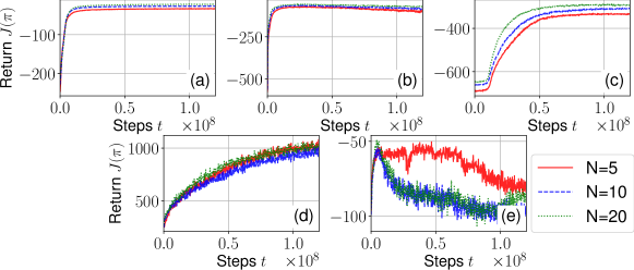
Figure 9: Training curves (mean episode return vs. time steps) of M3FPPO in red, trained on the finite systems with $N\in\{5,10,20\}$. (a) 2G; (b) Formation; (c) Beach Bar; (d) Foraging; (e) Potential.

References

- Anderson & Kurtz (2011) Anderson, D. F. and Kurtz, T. G. Continuous time Markov chain models for chemical reaction networks. In Design and analysis of biomolecular circuits, pp. 3–42. Springer, 2011.
- Bäuerle (2021) Bäuerle, N. Mean field Markov decision processes. arXiv:2106.08755, 2021.
- Bensoussan et al. (2013) Bensoussan, A., Frehse, J., Yam, P., et al. Mean field games and mean field type control theory, volume 101. Springer, 2013.
- Bernstein et al. (2002) Bernstein, D. S., Givan, R., Immerman, N., and Zilberstein, S. The complexity of decentralized control of Markov decision processes. Math. Oper. Res., 27(4):819–840, 2002.
- Billingsley (2013) Billingsley, P. Convergence of probability measures. John Wiley & Sons, 2013.
- Bonesini et al. (2022) Bonesini, O., Campi, L., and Fischer, M. Correlated equilibria for mean field games with progressive strategies. arXiv:2212.01656, 2022.
- Brockman et al. (2016) Brockman, G., Cheung, V., Pettersson, L., Schneider, J., Schulman, J., Tang, J., and Zaremba, W. Openai gym. arXiv:1606.01540, 2016.
- Cabannes et al. (2022) Cabannes, T., Laurière, M., Perolat, J., Marinier, R., Girgin, S., Perrin, S., Pietquin, O., Bayen, A. M., Goubault, E., and Elie, R. Solving n-player dynamic routing games with congestion: A mean-field approach. In Proc. AAMAS, volume 21, pp. 1557–1559, 2022.
- Caines & Huang (2019) Caines, P. E. and Huang, M. Graphon mean field games and the GMFG equations: -Nash equilibria. In Proc. IEEE CDC, pp. 286–292, 2019.
- Caines & Kizilkale (2016) Caines, P. E. and Kizilkale, A. C. -Nash equilibria for partially observed LQG mean field games with a major player. IEEE Trans. Automat. Contr., 62(7):3225–3234, 2016.
- Campi & Fischer (2022) Campi, L. and Fischer, M. Correlated equilibria and mean field games: a simple model. Math. Oper. Res., 2022.
- Cardaliaguet & Hadikhanloo (2017) Cardaliaguet, P. and Hadikhanloo, S. Learning in mean field games: the fictitious play. ESAIM Control Optim. Calc. Var., 23(2):569–591, 2017.
- Carmona (2020) Carmona, R. Applications of mean field games in financial engineering and economic theory. arXiv:2012.05237, 2020.
- Carmona et al. (2016) Carmona, R., Delarue, F., and Lacker, D. Mean field games with common noise. The Annals of Probability, 44(6):3740–3803, 2016.
- Carmona et al. (2018) Carmona, R., Delarue, F., et al. Probabilistic Theory of Mean Field Games with Applications I-II. Springer, 2018.
- Carmona et al. (2019) Carmona, R., Laurière, M., and Tan, Z. Model-free mean-field reinforcement learning: mean-field MDP and mean-field Q-learning. arXiv:1910.12802, 2019.
- Carmona et al. (2022) Carmona, R., Cormier, Q., and Soner, H. M. Synchronization in a Kuramoto mean field game. arXiv:2210.12912, 2022.
- Cui & Koeppl (2021) Cui, K. and Koeppl, H. Approximately solving mean field games via entropy-regularized deep reinforcement learning. In Proc. AISTATS, pp. 1909–1917, 2021.
- Cui & Koeppl (2022) Cui, K. and Koeppl, H. Learning graphon mean field games and approximate Nash equilibria. In Proc. ICLR, pp. 1–31, 2022.
- Cui et al. (2021) Cui, K., Tahir, A., Sinzger, M., and Koeppl, H. Discrete-time mean field control with environment states. In Proc. IEEE CDC, pp. 5239–5246, 2021.
- Daskalakis et al. (2009) Daskalakis, C., Goldberg, P. W., and Papadimitriou, C. H. The complexity of computing a Nash equilibrium. SIAM J. Comput., 39(1):195–259, 2009.
- de Witt et al. (2020) de Witt, C. S., Gupta, T., Makoviichuk, D., Makoviychuk, V., Torr, P. H., Sun, M., and Whiteson, S. Is independent learning all you need in the Starcraft multi-agent challenge? arXiv:2011.09533, 2020.
- DeVore & Lorentz (1993) DeVore, R. A. and Lorentz, G. G. Constructive approximation, volume 303. Springer Science & Business Media, 1993.
- Djehiche et al. (2017) Djehiche, B., Tcheukam, A., and Tembine, H. Mean-field-type games in engineering. AIMS Electronics and Electrical Engineering, 1(1):18–73, 2017.
- Dunyak & Caines (2021) Dunyak, A. and Caines, P. E. Large scale systems and SIR models: A featured graphon approach. In Proc. IEEE CDC, pp. 6928–6933. IEEE, 2021.
- Flamary et al. (2021) Flamary, R., Courty, N., Gramfort, A., Alaya, M. Z., Boisbunon, A., Chambon, S., Chapel, L., Corenflos, A., Fatras, K., Fournier, N., Gautheron, L., Gayraud, N. T., Janati, H., Rakotomamonjy, A., Redko, I., Rolet, A., Schutz, A., Seguy, V., Sutherland, D. J., Tavenard, R., Tong, A., and Vayer, T. Pot: Python optimal transport. J. Mach. Learn. Res., 22(78):1–8, 2021.
- Ganapathi Subramanian et al. (2020) Ganapathi Subramanian, S., Poupart, P., Taylor, M. E., and Hegde, N. Multi type mean field reinforcement learning. In Proc. AAMAS, volume 19, pp. 411–419, 2020.
- Ganapathi Subramanian et al. (2021) Ganapathi Subramanian, S., Taylor, M. E., Crowley, M., and Poupart, P. Partially observable mean field reinforcement learning. In Proc. AAMAS, volume 20, pp. 537–545, 2021.
- Gast & Gaujal (2011) Gast, N. and Gaujal, B. A mean field approach for optimization in discrete time. Discrete Event Dynamic Systems, 21(1):63–101, 2011.
- Gast & Van Houdt (2018) Gast, N. and Van Houdt, B. A refined mean field approximation. ACM SIGMETRICS Perform. Eval. Rev., 46(1):113–113, 2018.
- Gu et al. (2019) Gu, H., Guo, X., Wei, X., and Xu, R. Dynamic programming principles for mean-field controls with learning. arXiv:1911.07314, 2019.
- Gu et al. (2021) Gu, H., Guo, X., Wei, X., and Xu, R. Mean-field controls with Q-learning for cooperative MARL: convergence and complexity analysis. SIAM J. Math. Data Sci., 3(4):1168–1196, 2021.
- Guo et al. (2019) Guo, X., Hu, A., Xu, R., and Zhang, J. Learning mean-field games. In Proc. NeurIPS, pp. 4966–4976, 2019.
- Guo et al. (2022) Guo, X., Hu, A., Xu, R., and Zhang, J. A general framework for learning mean-field games. Math. Oper. Res., 2022.
- Gupta et al. (2017) Gupta, J. K., Egorov, M., and Kochenderfer, M. Cooperative multi-agent control using deep reinforcement learning. In Proc. AAMAS, pp. 66–83, 2017.
- Hernández-Lerma & Lasserre (2012) Hernández-Lerma, O. and Lasserre, J. B. Discrete-time Markov control processes: basic optimality criteria, volume 30. Springer Science & Business Media, 2012.
- Hernández-Lerma & Muñoz de Ozak (1992) Hernández-Lerma, O. and Muñoz de Ozak, M. Discrete-time Markov control processes with discounted unbounded costs: optimality criteria. Kybernetika, 28(3):191–212, 1992.
- Hu et al. (2022) Hu, Y., Wei, X., Yan, J., and Zhang, H. Graphon mean-field control for cooperative multi-agent reinforcement learning. arXiv:2209.04808, 2022.
- Huang et al. (2006) Huang, M., Malhamé, R. P., and Caines, P. E. Large population stochastic dynamic games: closed-loop McKean-Vlasov systems and the Nash certainty equivalence principle. Commun. Inf. Syst., 6(3):221–252, 2006.
- Kallenberg et al. (2017) Kallenberg, O. et al. Random measures, theory and applications, volume 1. Springer, 2017.
- Kiss et al. (2017) Kiss, I. Z., Miller, J. C., and Simon, P. L. Mathematics of Epidemics on Networks: From Exact to Approximate Models, volume 46. Springer, 2017. doi: 10.1007/978-3-319-50806-1.
- Lasry & Lions (2007) Lasry, J.-M. and Lions, P.-L. Mean field games. Japanese J. Math., 2(1):229–260, 2007.
- Laurière et al. (2022) Laurière, M., Perrin, S., Geist, M., and Pietquin, O. Learning mean field games: A survey. arXiv:2205.12944, 2022.
- Liang et al. (2018) Liang, E., Liaw, R., Nishihara, R., Moritz, P., Fox, R., Goldberg, K., Gonzalez, J., Jordan, M., and Stoica, I. RLlib: Abstractions for distributed reinforcement learning. In Proc. ICML, pp. 3053–3062, 2018.
- Liu et al. (2022) Liu, X., Wei, H., and Ying, L. Scalable and sample efficient distributed policy gradient algorithms in multi-agent networked systems. arXiv:2212.06357, 2022.
- Mondal et al. (2022) Mondal, W. U., Agarwal, M., Aggarwal, V., and Ukkusuri, S. V. On the approximation of cooperative heterogeneous multi-agent reinforcement learning (MARL) using mean field control (MFC). J. Mach. Learn. Res., 23(129):1–46, 2022.
- Mondal et al. (2023) Mondal, W. U., Aggarwal, V., and Ukkusuri, S. V. Mean-field control based approximation of multi-agent reinforcement learning in presence of a non-decomposable shared global state. arXiv:2301.06889, 2023.
- Motte & Pham (2022a) Motte, M. and Pham, H. Mean-field Markov decision processes with common noise and open-loop controls. The Annals of Applied Probability, 32(2):1421–1458, 2022a.
- Motte & Pham (2022b) Motte, M. and Pham, H. Quantitative propagation of chaos for mean field Markov decision process with common noise. arXiv:2207.12738, 2022b.
- Muller et al. (2021) Muller, P., Rowland, M., Elie, R., Piliouras, G., Perolat, J., Lauriere, M., Marinier, R., Pietquin, O., and Tuyls, K. Learning equilibria in mean-field games: Introducing mean-field PSRO. In Proc. AAMAS, volume 20, pp. 926–934, 2021.
- Nourian & Caines (2013) Nourian, M. and Caines, P. E. -Nash mean field game theory for nonlinear stochastic dynamical systems with major and minor agents. SIAM J. Contr. Optim., 51(4):3302–3331, 2013.
- Oliehoek & Amato (2016) Oliehoek, F. A. and Amato, C. A Concise Introduction to Decentralized POMDPs. Springer, 2016.
- Ouyang et al. (2022) Ouyang, L., Wu, J., Jiang, X., Almeida, D., Wainwright, C. L., Mishkin, P., Zhang, C., Agarwal, S., Slama, K., Ray, A., et al. Training language models to follow instructions with human feedback. arXiv:2203.02155, 2022.
- Papoudakis et al. (2021) Papoudakis, G., Christianos, F., Schäfer, L., and Albrecht, S. V. Benchmarking multi-agent deep reinforcement learning algorithms in cooperative tasks. In Proc. NeurIPS Track Datasets Benchmarks, 2021.
- Parthasarathy (2005) Parthasarathy, K. R. Probability measures on metric spaces, volume 352. American Mathematical Soc., 2005.
- Pasztor et al. (2021) Pasztor, B., Bogunovic, I., and Krause, A. Efficient model-based multi-agent mean-field reinforcement learning. arXiv:2107.04050, 2021.
- Pérolat et al. (2022) Pérolat, J., Perrin, S., Elie, R., Laurière, M., Piliouras, G., Geist, M., Tuyls, K., and Pietquin, O. Scaling mean field games by online mirror descent. In Proc. AAMAS, volume 21, pp. 1028–1037, 2022.
- Perrin et al. (2020) Perrin, S., Pérolat, J., Laurière, M., Geist, M., Elie, R., and Pietquin, O. Fictitious play for mean field games: Continuous time analysis and applications. In Proc. NeurIPS, volume 33, pp. 13199–13213, 2020.
- Perrin et al. (2022) Perrin, S., Laurière, M., Pérolat, J., Élie, R., Geist, M., and Pietquin, O. Generalization in mean field games by learning master policies. In Proc. AAAI, volume 36, pp. 9413–9421, 2022.
- Pham & Wei (2018) Pham, H. and Wei, X. Bellman equation and viscosity solutions for mean-field stochastic control problem. ESAIM Contr. Optim. Calc. Var., 24(1):437–461, 2018.
- Qu et al. (2020a) Qu, G., Lin, Y., Wierman, A., and Li, N. Scalable multi-agent reinforcement learning for networked systems with average reward. In Proc. NeurIPS, volume 33, pp. 2074–2086, 2020a.
- Qu et al. (2020b) Qu, G., Wierman, A., and Li, N. Scalable reinforcement learning of localized policies for multi-agent networked systems. In Proc. Learn. Dyn. Contr., pp. 256–266, 2020b.
- Saldi et al. (2018) Saldi, N., Başar, T., and Raginsky, M. Markov–Nash equilibria in mean-field games with discounted cost. SIAM J. Contr. Optim., 56(6):4256–4287, 2018.
- Saldi et al. (2019) Saldi, N., Başar, T., and Raginsky, M. Partially-observed discrete-time risk-sensitive mean-field games. In Proc. IEEE CDC, pp. 317–322, 2019.
- Sanjari & Yüksel (2020) Sanjari, S. and Yüksel, S. Optimal solutions to infinite-player stochastic teams and mean-field teams. IEEE Trans. Automat. Contr., 66(3):1071–1086, 2020.
- Schrittwieser et al. (2020) Schrittwieser, J., Antonoglou, I., Hubert, T., Simonyan, K., Sifre, L., Schmitt, S., Guez, A., Lockhart, E., Hassabis, D., Graepel, T., et al. Mastering atari, go, chess and shogi by planning with a learned model. Nature, 588(7839):604–609, 2020.
- Schulman et al. (2017) Schulman, J., Wolski, F., Dhariwal, P., Radford, A., and Klimov, O. Proximal policy optimization algorithms. arXiv:1707.06347, 2017.
- Şen & Caines (2014) Şen, N. and Caines, P. E. Mean field games with partially observed major player and stochastic mean field. In Proc. IEEE CDC, pp. 2709–2715, 2014.
- Şen & Caines (2016) Şen, N. and Caines, P. E. Mean field game theory with a partially observed major agent. SIAM J. Contr. Optim., 54(6):3174–3224, 2016.
- Şen & Caines (2019) Şen, N. and Caines, P. E. Mean field games with partial observation. SIAM J. Contr. Optim., 57(3):2064–2091, 2019.
- Shiri et al. (2019) Shiri, H., Park, J., and Bennis, M. Massive autonomous UAV path planning: A neural network based mean-field game theoretic approach. In Proc. IEEE GLOBECOM, pp. 1–6. IEEE, 2019.
- Subramanian et al. (2022) Subramanian, S. G., Taylor, M. E., Crowley, M., and Poupart, P. Decentralized mean field games. In Proc. AAAI, volume 36, pp. 9439–9447, 2022.
- Sznitman (1991) Sznitman, A.-S. Topics in propagation of chaos. In Ecole d’été de probabilités de Saint-Flour XIX—1989, pp. 165–251. Springer, 1991.
- Tan (1993) Tan, M. Multi-agent reinforcement learning: Independent vs. cooperative agents. In Proc. ICML, pp. 330–337, 1993.
- Tchuendom et al. (2021) Tchuendom, R. F., Caines, P. E., and Huang, M. Critical nodes in graphon mean field games. In Proc. IEEE CDC, pp. 166–170. IEEE, 2021.
- Villani (2009) Villani, C. Optimal transport: old and new, volume 338. Springer, 2009.
- Vinyals et al. (2019) Vinyals, O., Babuschkin, I., Czarnecki, W. M., Mathieu, M., Dudzik, A., Chung, J., Choi, D. H., Powell, R., Ewalds, T., Georgiev, P., et al. Grandmaster level in StarCraft II using multi-agent reinforcement learning. Nature, 575(7782):350–354, 2019.
- Yang et al. (2018) Yang, Y., Luo, R., Li, M., Zhou, M., Zhang, W., and Wang, J. Mean field multi-agent reinforcement learning. In Proc. ICML, pp. 5571–5580, 2018.
- Yardim et al. (2022) Yardim, B., Cayci, S., Geist, M., and He, N. Policy mirror ascent for efficient and independent learning in mean field games. arXiv:2212.14449, 2022.
- Yu et al. (2022) Yu, C., Velu, A., Vinitsky, E., Gao, J., Wang, Y., Bayen, A., and Wu, Y. The surprising effectiveness of PPO in cooperative multi-agent games. In Proc. NeurIPS Datasets and Benchmarks, 2022.
- Zhang et al. (2021) Zhang, K., Yang, Z., and Başar, T. Multi-agent reinforcement learning: A selective overview of theories and algorithms. In Vamvoudakis, K. G., Wan, Y., Lewis, F. L., and Cansever, D. (eds.), Handbook of Reinforcement Learning and Control, pp. 321–384. Springer International Publishing, Cham, 2021.