Conformal bootstrap in momentum space at finite volume

Kanade Nishikawa

Kavli Institute for the Physics and Mathematics of the Universe (WPI),
the University of Tokyo Kashiwa-no-ha, Chiba 277-8583, Japan

In this paper, we Fourier transform the Wightman function concerning energy and angular momentum on the $S^{D-1}$ spatial slice in radial quantization in $D=2,3$ dimensions. In each case, we use the conformal Ward Identities to solve systematically for the Fourier components. We then use these Fourier components to build conformal blocks for the four-point function in momentum space, giving a finite-volume version of the momentum-space conformal blocks. We check that this construction is consistent with the known result in infinite volume. Our construction may help to find bootstrap equations that can give nontrivial constraints that do not appear in analysis in infinite volume. We show some examples of bootstrap equations and their nontriviality.

1 Introduction

The conformal bootstrap method was applied by the paper [BPZ84] to solve an infinite class of two-dimensional conformal field theories (CFTs). Now, it is known as one of the most influential and fascinating tools to analyze CFT from the point of nonperturbative aspects of the theory. It carves out the space of consistent CFTs by imposing physical conditions such as symmetry, causality, and unitarity. It leads to nontrivial conditions that cannot be obtained from the algebraic structure of conformal algebra and perturbative analysis. About thirty years after their work [BPZ84], the paper [RRTV08] introduced the numerical method for conformal bootstrap equations to get constraints for higher-dimensional CFTs. Using crossing symmetry for the four-point function, they showed the upper bound on the conformal dimension of the first scalar appearing in the Operator Product Expansion (OPE) of two identical scalars. After their work, much progress has been made, such as fixing the critical exponents of the Ising model in three-dimensional CFT [ESPP⁺12, ESPP⁺14, KPSD14b, KPSDV15, KPSD14a, KPSDV16, SD15] and getting bounds on the scaling dimensions of the theory with global $O(N)$ symmetry [KPSD14b, KPSDV15, KPSDV16, NO14]. Please see the reviews [PSD16, PRV19, Che19] to check the recent works in conformal bootstrap.

As numerical bootstrap methods developed, there was a growing body of research investigating the analytical properties of bootstrap. One of the current research directions on conformal bootstrap is large N expansion. This analysis method is robust in AdS/CFT correspondence [Mal98, GKP98, Wit98, HPPS09], in which we have a good correspondence between weakly coupled gravity in AdS and its dual CFTs. “Weakly coupled” translates to the CFT with large N, and in addition, we demand that CFT on the boundary is strongly coupled to make the gravity theories on the bulk without light particles of spin greater than two. In the analysis, we perturb the CFT by $1/N$ and $1/\Delta$, where $\Delta$ is the conformal dimension of the lightest operator in the CFT. Many researchers have studied the relationship between weakly coupled bulk theory and CFT data on its boundary [AABP17, ADHP18, ACH18, AB17, RZ17, RZ18, CHT19]. The conformal bootstrap helps obtain consistent theories of gravity in AdS from the effective field theories, the swampland program [Vaf05, AHMNV07, Pal19]. In AdS/CFT correspondence, the AdS cylinder in global coordinates corresponds to the boundary CFT in radial quantization. With these physical motivations, formulating conformal bootstrap at finite volume on the cylinder is naturally needed to understand the bulk theory.

Recently, CFT in momentum space has been developed formally in [Gil20, CDRMS13, BMS14, INT19, BG20]. Those papers define correlation functions in momentum space as a Fourier transform of that in position space. CFT in momentum space has physical applications such as the study of anomalies [GM09, Mot10, ACDR09, ACDR10a, ACDR10b, CDRQS11, CDRS11], the determination of the form of conformal invariance in the non-Gaussian features of the cosmic microwave background [AMM97, AMM12], and an investigation for inflation [MP11, KR12].

One of the difficulties of analysis in momentum space is that we cannot expect the time-ordered correlation function to behave well because the integral calculation in the Fourier transform involves the position where the operators are not time-ordered. Instead, the Wightman function is a good function for the analysis in momentum space. The Wightman function has an operator algebra, but we have yet to study its structure so much. The conclusion and discussion summarize the future direction that surveys algebraic construction in momentum space.

When studying CFT in radial quantization, we can expect that the analysis in momentum space is the most suitable because the feature of CFT in radial quantization is that the energy and momentum are quantized. So, studying CFT in momentum space is natural if we try to find the difference between CFT in $\mathbb{R}^{1,d-1}$, and CFT in $\mathbb{R}\times S^{d-1}$.

From those considerations, we formulate the basis for the conformal bootstrap in momentum space using the Wightman function at finite volume in this paper. We expect that the conformal bootstrap at finite volume gives constraints for CFT data that cannot be obtained in CFT at infinite volume. In this paper, we show that the two- and three-point function at finite volume leads to that at infinite volume under the “Large volume limit.” It implies that the information in conformal bootstrap at finite volume is richer than that at infinite volume. As an analysis method that is particular for CFT at finite volume, we consider expansion by $1/R$, where $R$ is a compactification radius. We leave this kind of analysis to future work.

This paper is organized as follows. We summarize the result in two-dimensional CFT in section 2. We compute two- and three-point functions in momentum space with Ward Identities (WIs). This method is powerful because it applies to general operators and is helpful for computational calculation. In section 3, we study three-dimensional CFT by using WIs. Though we cannot get a closed form for the three-point function, ODEs obtained from WIs may be helpful for calculation with a computer. Finally, we show one of the applications of our calculation result. We develop bootstrap equations by using improved microcausality conditions. It was designed in infinite volume in the paper [GLLM20]. We resolve some problems and get a proper bootstrap equation in finite volume. Though our development is incomplete, it implies that the bootstrap method in momentum space might be helpful. We leave the problem for future work.

2 Main results in $D=2$

This section summarizes the derivation of two- and three-point Wightman functions in two-dimensional momentum space. We deal with CFT quantized on a cylinder.

For two-dimensional CFT, the factorization method is potent as we can independently calculate holomorphic and antiholomorphic parts. After that, we can construct complete correlation functions for general operators.

There are three ways to get them. The first is a direct integral calculation, which is easy for a simple case, but an analytic continuation for general situations is not trivial.

On the other hand, the Ward Identity (WI) method is helpful for the general case, which is the second procedure. Though solving the ODEs obtained from WI is a little tricky for three-point functions, this method emphasizes that we can determine all of the correlation functions of the mode operator from ones including only primaries.

The third procedure is an algebraic construction, which helps construct a completeness relation when calculating a four-point function.

The most crucial difference between two-dimensional CFT and higher-dimensional CFT is that there are Virasoro descendants in the two-dimensional CFT. In this paper, we call the descendants made by acting $L_{-1}$s on primaries as “descendants” and the descendants made by working $L_{-n}\ (n\geq 2)$s on primaries as “Virasoro descendants.” When considering four-point functions in momentum space, we do not have to consider descendants, but we cannot ignore the contributions from Virasoro descendants. We will see the calculation in the latter chapter. We summarize the results briefly, so please visit the appendix for a more detailed analysis and supplements.

2.1 Conformal generators and their action

We use cylinder coordinates and complex plane coordinates. In the complex plane, we use $z$ and $\bar{z}$ as coordinates, and $\omega=\sigma_{1}+i\sigma_{2}=\sigma-i\tau$ and $\bar{\omega}=\sigma_{1}-i\sigma_{2}=\sigma+i\tau$ for the cylinder frame. They are related to each other by conformal transformations with radius $R$.

$$z=re^{i\theta}=Re^{\frac{i\omega}{R}}=Re^{\frac{i\sigma+\tau}{R}},\hskip 28.45274pt\bar{z}=re^{-i\theta}=Re^{-\frac{i\bar{\omega}}{R}}=Re^{\frac{-i\sigma+\tau}{R}}$$ (2.1)

We define two “Spatially-integrated mode” types for primary operators. The first one is

$$\tilde{\mathcal{O}}_{n}(r)\equiv\int_{C_{r}}\frac{\differential{\theta}}{2\pi}\mathcal{O}(r,\theta)e^{-in\theta},$$ (2.2)

where the integral path $C_{r}$ is the circumference of radius $r$. And the second one is defined for holomorphic operators $\mathcal{O}(z)$ and antiholomorphic operators $\bar{\mathcal{O}}(\bar{z})$, respectively.

$$\mathcal{O}_{n}\equiv\frac{1}{2\pi i}\oint\frac{\differential{z}}{z^{1+n}}\mathcal{O}(z),\hskip 28.45274pt\bar{\mathcal{O}}_{n}\equiv\frac{1}{2\pi i}\oint\frac{\differential{\bar{z}}}{\bar{z}^{1+n}}\bar{\mathcal{O}}(\bar{z})$$ (2.3)

For example, for holomorphic operators, $\tilde{\mathcal{O}}_{n}(r)=r^{n}\mathcal{O}_{n}$. For operators with spin $s$, we also use other types of representation. Define $J\equiv n+s$ and $\bar{J}\equiv-n-s$, then

$$\mathcal{O}_{[J]}\equiv\mathcal{O}_{n},\hskip 28.45274pt\bar{\mathcal{O}}_{[\bar{J}]}\equiv\bar{\mathcal{O}}_{n}.$$ (2.4)

We obtain the action of the conformal generators on these modes. For example,

$$P_{z}\cdot\tilde{\mathcal{O}}_{n}=\frac{1}{2}\int\frac{\differential{\theta}}{2\pi}\left(\partial_{r}\mathcal{O}-\frac{i}{r}\partial_{\theta}\mathcal{O}\right)e^{-i(n+1)\theta}=\frac{1}{2}\left(\partial_{r}+\frac{n+1}{r}\right)\tilde{\mathcal{O}}_{n+1}=\frac{1}{2r}\left(\hat{E}+n+1\right)\tilde{\mathcal{O}}_{n+1},$$ (2.5)

where $\hat{E}=r\partial_{r}$. Similarly, we get the following equations.

$$P_{\bar{z}}\cdot\tilde{\mathcal{O}}_{n} =\frac{1}{2}\left(\partial_{r}-\frac{n-1}{r}\right)\tilde{\mathcal{O}}_{n-1}=\frac{1}{2r}\left(\hat{E}-n+1\right)\tilde{\mathcal{O}}_{n-1}$$ (2.6)

$$K^{z}\cdot\tilde{\mathcal{O}}_{n} =\frac{r^{2}}{2}\left(\partial_{r}+\frac{n-1}{r}\right)\tilde{\mathcal{O}}_{n-1}+2hr\tilde{\mathcal{O}}_{n-1}=\frac{r}{2}\left(\hat{E}+n+4h-1\right)\tilde{\mathcal{O}}_{n-1}$$ (2.7)

$$K^{\bar{z}}\cdot\tilde{\mathcal{O}}_{n} =\frac{r^{2}}{2}\left(\partial_{r}-\frac{n+1}{r}\right)\tilde{\mathcal{O}}_{n+1}+2\tilde{h}r\tilde{\mathcal{O}}_{n+1}=\frac{r}{2}\left(\hat{E}-n+4\tilde{h}-1\right)\tilde{\mathcal{O}}_{n+1}$$ (2.8)

$$L_{0}\cdot\tilde{\mathcal{O}}_{n} =\frac{1}{2}\left(r\partial_{r}+n+2h\right)\tilde{\mathcal{O}}_{n}=\frac{1}{2}\left(\hat{E}+n+2h\right)\tilde{\mathcal{O}}_{n}$$ (2.9)

$$\tilde{L}_{0}\cdot\tilde{\mathcal{O}}_{n} =\frac{1}{2}\left(r\partial_{r}-n+2\tilde{h}\right)\tilde{\mathcal{O}}_{n}=\frac{1}{2}\left(\hat{E}-n+2\tilde{h}\right)\tilde{\mathcal{O}}_{n}$$ (2.10)

2.2 Two-point function

2.2.1 Two-point function for primaries

Define the complete Wightman two-point function of primaries as

$$C(n_{1},n_{2},r_{1},r_{2})\equiv\langle\tilde{\mathcal{O}}_{n_{2}}^{(2)}(r_{2})\tilde{\mathcal{O}}_{n_{1}}^{(1)}(r_{1})\rangle\equiv\delta(n_{1}+n_{2}+s_{1}+s_{2})r_{1}^{-\Delta_{1}}r_{2}^{-\Delta_{2}}F_{n_{1}}(y),$$ (2.11)

where $y\equiv r_{1}/r_{2}$ is a ratio of radius. We used $L_{0}$ and $\tilde{L}_{0}$ WIs to get the reduced form. Usually, the above delta function means Dirac’s delta function, but in this paper, it often means $0$ or $1$ function when its content has a discrete value.

$$\delta(x)\equiv\begin{cases}1&\text{if $x=0$}\\ 0&\text{otherwise}\end{cases}$$ (2.12)

For this reduced form, we get WIs, which give ODEs for a two-point function. Four are left, as we used two of six WIs to get the reduced form.

$$L_{-1} :\left(y\derivative{y}-\Delta_{1}+n+1\right)F_{n+1}(y)+y\left(-y\derivative{y}-\Delta_{2}-n-s_{1}-s_{2}\right)F_{n}(y)=0$$ (2.13)

$$\tilde{L}_{-1} :y\left(-y\derivative{y}-\Delta_{2}+n+1+s_{1}+s_{2}\right)F_{n+1}(y)+\left(y\derivative{y}-\Delta_{1}-n\right)F_{n}(y)=0$$ (2.14)

$$L_{1} :\left(-y\derivative{y}+\Delta_{2}-n-1-s_{1}+s_{2}\right)F_{n+1}(y)+y\left(y\derivative{y}+\Delta_{1}+2s_{1}+n\right)F_{n}(y)=0$$ (2.15)

$$\tilde{L}_{1} :y\left(y\derivative{y}+\Delta_{1}-2s_{1}-n-1\right)F_{n+1}(y)+\left(-y\derivative{y}+\Delta_{2}+n+s_{1}-s_{2}\right)F_{n}(y)=0$$ (2.16)

The solution of these ODEs is as follows.

$$G_{n+s} \equiv F_{n}=K_{s}y^{\Delta+|n|}(\sum_{l=0}c_{n+s|l}y^{2l})$$ (2.17)

$$c_{n+s|l} =\frac{\Gamma(\Delta+s+l+n)\Gamma(\Delta-s+l)}{\Gamma(\Delta+s)\Gamma(\Delta-s)\Gamma(l+n+1)\Gamma(l+1)}$$ (2.18)

$K_{s}$ is an undetermined constant depending on the normalization of operators. The appendix summarizes how to solve these WIs and checks that this solution matches that obtained by a direct integral.

In the two-point function, $\Delta+s=h$ and $\Delta-s=\tilde{h}$ appear independently. In other words, we can factorize it into holomorphic and antiholomorphic parts. It is natural, but we summarize it to clarify the situation. Let us perform the Fourier transform of the two-point function of scalar operators with the above solution.

$$\int\frac{\differential\theta_{1}}{2\pi}\frac{\differential\theta_{2}}{2\pi}e^{-in_{1}\theta_{1}-in_{2}\theta_{2}}\langle\mathcal{O}^{(2)}\mathcal{O}^{(1)}\rangle=\delta(n_{1}+n_{2})r_{2}^{-2\Delta}\sum_{l=0}\frac{\Gamma(\Delta+l+n_{1})\Gamma(\Delta+l)}{\Gamma(l+n_{1}+1)\Gamma(l+1)\Gamma(\Delta)^{2}}\left(\frac{r_{1}}{r_{2}}\right)^{2l+n_{1}}$$ (2.19)

The operator normalisation has been chosen to set $K_{s}$ to unity. The coordinate transformation from the complex plane to the cylinder, inverse Wick rotation, and complete Fourier transform give

$$\int\frac{\differential\sigma_{1}}{2\pi R}\int\frac{\differential\sigma_{2}}{2\pi R}\int\frac{\differential t_{1}}{2\pi}\int\frac{\differential t_{2}}{2\pi}e^{-iE_{1}t_{1}}e^{-iE_{2}t_{2}}e^{-i\sigma_{1}\frac{n_{1}}{R}}e^{-i\sigma_{2}\frac{n_{2}}{R}}\langle\mathcal{O}^{(2)}(\sigma_{2},\tau_{2})\mathcal{O}^{(1)}(\sigma_{1},\tau_{1})\rangle\\ =\delta(k_{1}+k_{2})\delta(E_{1}+E_{2})\frac{R^{-2\Delta}}{(\Gamma(\Delta))^{2}}\frac{\Gamma\left(\frac{R(E_{1}-k_{1})+\Delta}{2}\right)\Gamma\left(\frac{R(E_{1}+k_{1})+\Delta}{2}\right)}{\Gamma\left(\frac{R(E_{1}-k_{1})-\Delta}{2}+1\right)\Gamma\left(\frac{R(E_{1}+k_{1})-\Delta}{2}+1\right)}.$$ (2.20)

The point is that we can factorize the two-point function in momentum space into $E_{1}\pm k_{1}$ parts. It indicates that we can calculate it by multiplying the results in holomorphic and antiholomorphic parts, but what is the procedure? For holomorphic operators,

$$\int\frac{d\theta_{1}}{2\pi}\frac{d\theta_{2}}{2\pi}e^{-in_{1}\theta_{1}-in_{2}\theta_{2}}\langle\mathcal{O}^{(2)}\mathcal{O}^{(1)}\rangle\propto r_{1}^{-h}r_{2}^{-h}\delta(n_{1}+n_{2}+2h)\frac{\Gamma(n_{1}+2h)}{\Gamma(n_{1}+1)\Gamma(2h)}\left(\frac{r_{1}}{r_{2}}\right)^{n_{1}+h}.$$ (2.21)

And for antiholomorphic operators,

$$\int\frac{d\theta_{1}}{2\pi}\frac{d\theta_{2}}{2\pi}e^{i\bar{n}_{1}\theta_{1}+i\bar{n}_{2}\theta_{2}}\langle\mathcal{\bar{O}}^{(2)}\mathcal{\bar{O}}^{(1)}\rangle\propto r_{1}^{-\tilde{h}}r_{2}^{-\tilde{h}}\delta(\bar{n}_{1}+\bar{n}_{2}+2\tilde{h})\frac{\Gamma(\bar{n}_{1}+2\tilde{h})}{\Gamma(\bar{n}_{1}+1)\Gamma(2\tilde{h})}\left(\frac{r_{1}}{r_{2}}\right)^{\bar{n}_{1}+\tilde{h}}.$$ (2.22)

Multiplying them doesn’t give (2.20). The physical states created by $\tilde{O}_{n_{1}}$ are ones with spin $n_{1}$, so they have the form $(P_{z})^{n_{1}+l_{1}}(P_{\bar{z}})^{l_{1}}\ket{\Phi}$ with some integer $l_{1}$, where $\ket{\Phi}$ is a primary state created by inserting primary operator with conformal weight $(h,\tilde{h})$.

For this state, $n_{1}$ in (2.21) should be replaced by $n_{1}+l_{1}$, and $\bar{n}_{1}$ in (2.22) should be replaced by $l_{1}$. From here, we only concentrate on the Gamma function dependent part in the two-point function since the delta functional part and $r_{1},r_{2}$ dependent part only give conservation law.

The multiplication of the holomorphic part and the antiholomorphic part gives

$$\frac{\Gamma(n_{1}+2h+l_{1})}{\Gamma(n_{1}+l_{1}+1)\Gamma(2h)}\frac{\Gamma(l_{1}+2h)}{\Gamma(l_{1}+1)\Gamma(2h)}=\frac{\Gamma(\Delta+n_{1}+l_{1})}{\Gamma(n_{1}+l_{1}+1)\Gamma(\Delta)}\frac{\Gamma(\Delta+l_{1})}{\Gamma(l_{1}+1)\Gamma(\Delta)}.$$ (2.23)

Energy for the state $(P_{z})^{n_{1}+l_{1}}(P_{\bar{z}})^{l_{1}}\ket{\Phi}$ is $E_{1}=(h+\tilde{h}+n_{1}+l_{1}+l_{1})/R=(\Delta+n_{1}+2l_{1})/R$ and momentum for the state is $k_{1}=n_{1}/R$. So, the Gamma function dependent part is

$$\frac{1}{(\Gamma(\Delta))^{2}}\frac{\Gamma\left(\frac{R(E_{1}-k_{1})+\Delta}{2}\right)\Gamma\left(\frac{R(E_{1}+k_{1})+\Delta}{2}\right)}{\Gamma\left(\frac{R(E_{1}-k_{1})-\Delta}{2}+1\right)\Gamma\left(\frac{R(E_{1}+k_{1})-\Delta}{2}+1\right)}.$$ (2.24)

It is the same as (2.20).

In the above example, we calculated the two-point function of scalar operators: direct integral calculation and factorization. Their results are the same, and we can generalize this method for other two-point functions. We will show more clearly that we can use the factorization method to calculate three-point functions later, and the logic is the same.

2.2.2 Two-point function for descendants

As well known, inserting descendant fields in the correlation function means acting differential operators on others.

$$\langle(L_{-m}\phi)(z)\phi_{1}(z_{1})\cdots\phi_{N}(z_{N})\rangle=\sum_{i=1}^{N}\left[\frac{(m-1)h_{i}}{(z_{i}-z)^{m}}-\frac{1}{(z_{i}-z)^{m-1}}\partialderivative{z_{i}}\right]\langle\phi(z)\phi_{1}(z_{1})\cdots\phi_{N}(z_{N})\rangle$$ (2.25)

So, for example,

$$\langle\phi_{[-J]}(L_{-m}\phi)_{[J]}\rangle =\oint\frac{dz_{2}}{z_{2}^{1-J-h}}\oint\frac{dz_{1}}{z_{1}^{1+J-h-m}}\left[\frac{(m-1)h}{(z_{2}-z_{1})^{m}}-\frac{1}{(z_{2}-z_{1})^{m-1}}\partialderivative{z_{2}}\right]\langle\phi(z_{2})\phi(z_{1})\rangle$$

$$=(m+1)h\frac{\Gamma(J+h)}{\Gamma(1+J-h-m)\Gamma(2h+m)}.$$ (2.26)

In general,

$$\langle\phi_{[-J]}(L_{-m_{k}}\cdots L_{-m_{2}}L_{-m_{1}}\phi)_{[J]}\rangle=\frac{\prod_{i=1}^{k}\left[(m_{i}+1)h+\sum_{j=1}^{i-1}m_{j}\right]\Gamma(J+h)}{\Gamma(1+J-h-\sum_{i=1}^{k}m_{i})\Gamma(2h+\sum_{i=1}^{k}m_{i})}.$$ (2.27)

For more general calculations such as $\langle(L_{-2}\phi)_{[-J]}(L_{-3}\phi)_{[J]}\rangle$, we also need to consider more complicated calculation including OPEs between energy-momentum tensors. Although one can compute an arbitrary correlation function in momentum space by a straightforward analysis, we can understand it more simply by using the algebraic method described next.

2.2.3 Algebraic construction

Like CFT in position space, we can calculate the two-point function by algebraic calculation. In the procedure, we consider in-state and out-state naturally, which is useful when constructing the completeness relation to calculate a four-point function.

As we can calculate the holomorphic and antiholomorphic parts independently, we only focus on the holomorphic part. First, the ket $\ket{\phi_{[J]}}$ is defined as

$$\ket{\phi_{[J]}}=\oint\frac{dz}{z^{1+J-h}}\phi(z)\ket{0}=\oint\frac{dz}{z^{1+J-h}}e^{iL_{-1}z}\phi(0)e^{-iL_{-1}z}\ket{0}=\frac{i^{J-h}}{(J-h)!}L_{-1}^{J-h}\ket{h}.$$ (2.28)

The ket for descendant field $(L_{-m_{k}}\cdots L_{-m_{2}}L_{-m_{1}}\phi)(z)$ is

$$\ket{L_{-m_{k}}\cdots L_{-m_{2}}L_{-m_{1}}\phi_{[J]}}=\frac{i^{J-h}}{(J-h)!}L_{-1}^{J-h}L_{-m_{k}}\cdots L_{-m_{2}}L_{-m_{1}}\ket{h}.$$ (2.29)

In this paper, we arrange the Virasoro generators so that $m_{1}\geq m_{2}\geq\cdots\geq m_{k}$ is satisfied.

We define the bra for the primary field and for the descendant field as

$$\bra{\phi_{[J]}}=\oint\frac{dz}{z^{1-J-h}}\frac{1}{z^{2h}}\bra{0}\phi(\infty)e^{-iL_{1}\frac{1}{z}}=\frac{(-i)^{J-h}}{(J-h)!}\bra{h}L_{1}^{J-h}$$ (2.30)

$$\bra{L_{-m_{k}}\cdots L_{-m_{2}}L_{-m_{1}}\phi_{[J]}}=\frac{(-i)^{J-h}}{(J-h)!}\bra{h}L_{m_{1}}L_{m_{2}}\cdots L_{m_{k}}L_{1}^{J-h}.$$ (2.31)

The phases are chosen so that $\bra{\phi_{[J]}}\ket{\phi_{[J]}}\geq 0$ and $\bra{L_{-m_{k}}\cdots L_{-m_{1}}\phi_{[J]}}\ket{L_{-m_{k}}\cdots L_{-m_{1}}\phi_{[J]}}\geq 0$ are satisfied. With those definitions, we can recover the previous result, for example,

$$\langle\phi_{[-h-2]}\phi_{[h+2]}\rangle=\frac{\Gamma(2h+2)}{\Gamma(3)\Gamma(2h)}=\bra{\phi_{[h+2]}}\ket{\phi_{[h+2]}}=\frac{1}{2!}\frac{1}{2!}\bra{h}L_{1}^{2}L_{-1}^{2}\ket{h}=h(2h+1).$$ (2.32)

This algebraic construction helps make a completeness relation needed to calculate the four-point function by conformal block decomposition. We will deal with it later.

2.2.4 Large volume limit for two-point function

In Gillioz’s paper [Gil21], they calculated the two-point function of scalars in momentum space in $d$-dimensional Minkowski space. They defined the double bracket notation as

$$\bra{0}\phi_{1}(k_{1})\cdots\phi_{n}(k_{n})\ket{0}=(2\pi)^{d}\delta^{d}(k_{1}+\cdots+k_{n})\llangle\phi_{1}(k_{1})\cdots\phi_{n}(k_{n})\rrangle.$$ (2.33)

Here, Fourier transform of operator $\tilde{\phi}(x)$ is $\phi(k)\equiv\int d^{d}xe^{ik\cdot x}\tilde{\phi}(x)$. So,

$$\llangle\phi_{1}(k_{1})\cdots\phi_{n}(k_{n})\rrangle=\int d^{d}x_{1}\cdots d^{d}x_{n-1}e^{i(k_{1}\cdot x_{1}+\cdots+k_{n-1}\cdot x_{n-1})}\bra{0}\tilde{\phi}_{1}(x_{1})\cdots\tilde{\phi}_{n}(0)\ket{0}.$$ (2.34)

The two-point function of the scalar operators for momentum $k$ lying in a forward light cone is

$$\llangle\phi(-k)\phi(k)\rrangle=\frac{(4\pi)^{d/2+1}}{2^{2\Delta+1}\Gamma(\Delta)\Gamma(\Delta-\frac{d}{2}+1)}(k^{2})^{\Delta-d/2}.$$ (2.35)

In two-dimensional spacetime,

$$\langle\phi_{1}(k_{1})\phi_{2}(k_{2})\rangle=(2\pi)^{2}\delta^{2}(k_{1}+k_{2})\frac{(4\pi)^{2}}{2^{2\Delta+1}(\Gamma(\Delta))^{2}}(k^{2})^{\Delta-1}.$$ (2.36)

We want this result by taking the limit of $R\rightarrow\infty$ for our result in finite volume. We call it “Large Volume Limit.” Our result is

$$\tilde{C}(k_{1},k_{2},E_{1},E_{2})\equiv\int\frac{dt_{1}}{2\pi}\frac{dt_{2}}{2\pi}\int\frac{d\sigma_{1}}{2\pi R}\frac{d\sigma_{2}}{2\pi R}e^{i\sigma_{1}k_{1}}e^{i\sigma_{2}k_{2}}e^{-it_{1}E_{1}}e^{-it_{2}E_{2}}\langle\phi_{2}(t_{2},\sigma_{2})\phi_{1}(t_{1},\sigma_{1})\rangle\\ =\delta(k_{1}+k_{2})\delta(E_{1}+E_{2})\frac{R^{-2\Delta}}{(\Gamma(\Delta))^{2}}\frac{\Gamma\left(\frac{R(E_{1}-k_{1})+\Delta}{2}\right)\Gamma\left(\frac{R(E_{1}+k_{1})+\Delta}{2}\right)}{\Gamma\left(\frac{R(E_{1}-k_{1})-\Delta}{2}+1\right)\Gamma\left(\frac{R(E_{1}+k_{1})-\Delta}{2}+1\right)}.$$ (2.37)

With Stirling’s approximation, we get

$$\lim_{R\rightarrow\infty}\text{(LHS)}\propto\delta(k_{1}+k_{2})^{2}\frac{R^{-2\Delta}}{\Gamma(\Delta)^{2}}\frac{(k_{1}-E_{1})^{\Delta-1}R^{\Delta}}{2^{\Delta-1}}\frac{(k_{1}+E_{1})^{\Delta-1}R^{\Delta}}{2^{\Delta-1}}\propto\delta(k_{1}+k_{2})^{2}\frac{(k^{2})^{\Delta-1}}{(\Gamma(\Delta))^{2}}.$$ (2.38)

This is identical to the result (2.36) at infinite volume calculated in the paper [Gil21].

2.3 Three-point function

Solving WIs for the three-point function is complicated. So first, we Fourier transform the three-point function of holomorphic operators directly and check that the solution satisfies the ODEs obtained from WIs. The three-point function of holomorphic operators is

$$\langle\mathcal{O}_{3}(z_{3})\mathcal{O}_{2}(z_{2})\mathcal{O}_{1}(z_{1})\rangle\equiv\lambda_{321}z_{21}^{h_{3}-h_{1}-h_{2}}z_{32}^{h_{1}-h_{3}-h_{2}}z_{31}^{h_{2}-h_{1}-h_{3}}\equiv\lambda_{321}z_{21}^{-b_{3}}z_{32}^{-b_{1}}z_{31}^{-b_{2}}.$$ (2.39)

Here, $h_{1},h_{2},h_{3}$ are conformal weight of operator $\mathcal{O}_{1},\mathcal{O}_{2},\mathcal{O}_{3}$. And we define $z_{ij}\equiv z_{i}-z_{j}$, $b_{1}\equiv h_{2}+h_{3}-h_{1}$, $b_{2}\equiv h_{1}+h_{3}-h_{2}$ and $b_{3}\equiv h_{1}+h_{2}-h_{3}$. We assume that conformal weights are all integers, but we can analytically continue the region of conformal weights by taking $n_{i}\ (i=1,2,3)$ non-integers. Then,

$$\langle\mathcal{O}_{n_{3}}\mathcal{O}_{n_{2}}\mathcal{O}_{n_{1}}\rangle=\frac{1}{(2\pi i)^{3}}\oint\frac{dz_{3}}{z_{3}^{1+n_{3}}}\oint\frac{dz_{2}}{z_{2}^{1+n_{2}}}\oint\frac{dz_{1}}{z_{1}^{1+n_{1}}}\langle\mathcal{O}_{3}(z_{3})\mathcal{O}_{2}(z_{2})\mathcal{O}_{1}(z_{1})\rangle\\ =\tfrac{\lambda_{321}\delta(\sum_{i=1}^{3}J_{i})}{\Gamma(b_{1})\Gamma(b_{2})\Gamma(b_{3})}\sum_{q=0}^{\mathrm{Min}\{n_{1},m_{3}\}}\tfrac{\Gamma[b_{3}+q+\mathrm{Max}\{{0,n_{1}-m_{3}}\}]\Gamma[b_{2}-q+\mathrm{Min}\{{n_{1},m_{3}}\}]\Gamma[b_{1}+q+\mathrm{Max}\{{m_{3}-n_{1},0}\}]}{\Gamma[1+q+\mathrm{Max}\{{0,n_{1}-m_{3}}\}]\Gamma[1-q+\mathrm{Min}\{{n_{1},m_{3}}\}]\Gamma[1+q+\mathrm{Max}\{{m_{3}-n_{1},0}\}]},$$ (2.40)

where $m_{3}=-(n_{3}+2h_{3})$. In the appendix, we summarize the detail of the derivation and check that the solution for the three-point function satisfies the ODEs obtained from WIs.

In the paper [Gil20] by Gillioz, they calculated the three-point function in infinite volume in the fully factorized form

$$\llangle\phi_{f}(p_{f})\phi_{0}(p_{0})\phi_{i}(p_{i})\rrangle=\lambda_{f0i}W(p_{f}^{+},p_{0}^{+},p_{i}^{+})W(p_{f}^{-},p_{0}^{-},p_{i}^{-}),$$ (2.41)

where $p^{\pm}=p_{0}\pm p_{1}$ and

$$W(p_{f}^{\pm},p_{0}^{\pm},p_{i}^{\pm})=\frac{(2\pi)^{2}}{2^{(\Delta_{f}+\Delta_{0}+\Delta_{i}-2)/2}}\frac{(p_{f}^{\pm})^{\Delta_{f}-d/2}(p_{i}^{\pm})^{\Delta_{i}-d/2}}{|p_{0}^{\pm}|^{(\Delta_{f}-\Delta_{0}+\Delta_{i})/2}}\\ \left[\frac{\Theta(p_{0}^{\pm})}{\Gamma(\Delta_{i})\Gamma\left(\frac{\Delta_{f}+\Delta_{0}-\Delta_{i}}{2}\right)}{}_{2}F_{1}\left(\frac{\Delta_{f}-\Delta_{0}+\Delta_{i}}{2},\frac{\Delta_{f}-\tilde{\Delta}_{0}+\Delta_{i}}{2};\Delta_{i};-\frac{p^{\pm}_{i}}{p^{\pm}_{0}}\right)\right.\\ \left.+\frac{\Theta(-p_{0}^{\pm})}{\Gamma(\Delta_{f})\Gamma\left(\frac{\Delta_{i}+\Delta_{0}-\Delta_{f}}{2}\right)}{}_{2}F_{1}\left(\frac{\Delta_{f}-\Delta_{0}+\Delta_{i}}{2},\frac{\Delta_{f}-\tilde{\Delta}_{0}+\Delta_{i}}{2};\Delta_{f};-\frac{p^{\pm}_{f}}{p^{\pm}_{0}}\right)\right].$$ (2.42)

Here, ${}_{2}F_{1}$ is a hypergeometric function

$${}_{2}F_{1}(a,b:c:z)=\sum_{n=0}^{\infty}\frac{(a)_{n}(b)_{n}}{(c)_{n}}\frac{z^{n}}{n!},$$ (2.43)

where $(a)_{n}$ is the Pochhammer symbol defined as follows.

$$(a)_{n}=\begin{cases}1&(n=0)\\ a(a+1)(a+2)\cdots(a+n-1)&(n>0)\end{cases}$$ (2.44)

We can see that the Wightman 3-point function is factorized into holomorphic and anti-holomorphic pieces, or equivalently into left- and right-movers.

We want to get this result by taking a large volume limit for our result at a finite volume. We use a time-reversal symmetric form for three-point functions. $\mathcal{K}_{\mathrm{red}}$ is defined as

$$\mathcal{K}(n_{1},n_{2},n_{3})\equiv\langle\mathcal{O}_{n_{3}}(z_{3})\mathcal{O}_{n_{2}}(z_{2})\mathcal{O}_{n_{1}}(z_{1})\rangle\equiv\delta(n_{1}+n_{2}+n_{3}+h_{1}+h_{2}+h_{3})\mathcal{K}_{\mathrm{red}}(n_{1},n_{3}).$$ (2.45)

And remember that this is equal to

$$\mathcal{K}_{\mathrm{red}}(n_{1},n_{3})\\ =\tfrac{\lambda_{321}}{\Gamma(b_{1})\Gamma(b_{2})\Gamma(b_{3})}\sum_{q=0}^{\mathrm{Min}\{n_{1},m_{3}\}}\tfrac{\Gamma[b_{3}+q+\mathrm{Max}\{{0,n_{1}-m_{3}}\}]\Gamma[b_{2}-q+\mathrm{Min}\{{n_{1},m_{3}}\}]\Gamma[b_{1}+q+\mathrm{Max}\{{m_{3}-n_{1},0}\}]}{\Gamma[1+q+\mathrm{Max}\{{0,n_{1}-m_{3}}\}]\Gamma[1-q+\mathrm{Min}\{{n_{1},m_{3}}\}]\Gamma[1+q+\mathrm{Max}\{{m_{3}-n_{1},0}\}]}.$$ (2.46)

To take a large volume limit, define $\mathcal{N}[x,y]\equiv\Gamma(1+x+y)/\Gamma(1+x)\Gamma(1+y)$. Under the $y\rightarrow\infty$ limit, $\mathcal{N}[x,y]\simeq y^{x}/\Gamma(1+x)$. With it, we can write a three-point function as

$$\mathcal{K}_{\mathrm{red}}(n_{1},n_{3})=\lambda_{321}\sum_{q=0}^{\mathrm{Min}\{n_{1},m_{3}\}}\mathcal{N}[b_{3}-1,q+\mathrm{Max}\{{0,n_{1}-m_{3}}\}]\\ \mathcal{N}[b_{2}-1,-q+\mathrm{Min}\{n_{1},m_{3}\}]\mathcal{N}[b_{1}-1,q+\mathrm{Max}\{m_{3}-n_{1},0\}].$$ (2.47)

Under a large volume limit, $n_{1}$ and $m_{3}$ also go to infinity. We define $\hat{q}\equiv q/R$, $\hat{n}_{1}\equiv n_{1}/R$, and $\hat{m}_{3}\equiv m_{3}/R$. Then, we get

$$\mathcal{N}[b_{1}-1,q+\mathrm{Max}\{m_{3}-n_{1},0\}]\simeq\frac{1}{\Gamma(b_{1})}(q+\mathrm{Max}\{m_{3}-n_{1},0\})^{b_{1}-1}$$ (2.48)

$$\mathcal{N}[b_{2}-1,-q+\mathrm{Min}\{n_{1},m_{3}\}]\simeq\frac{1}{\Gamma(b_{2})}(-q+\mathrm{Min}\{n_{1},m_{3}\})^{b_{2}-1}$$ (2.49)

$$\mathcal{N}[b_{3}-1,q+\mathrm{Max}\{{0,n_{1}-m_{3}}\}]\simeq\frac{1}{\Gamma(b_{3})}(q+\mathrm{Max}\{{0,n_{1}-m_{3}}\})^{b_{3}-1}.$$ (2.50)

The product is

$$\mathcal{N}[b_{1}-1,q+\mathrm{Max}\{m_{3}-n_{1},0\}]\mathcal{N}[b_{2}-1,-q+\mathrm{Min}\{n_{1},m_{3}\}]\mathcal{N}[b_{3}-1,q+\mathrm{Max}\{{0,n_{1}-m_{3}}\}]$$

$$=\left(\prod_{i=1}^{3}\tfrac{1}{\Gamma(b_{i})}\right)(q+\mathrm{Max}\{m_{3}-n_{1},0\})^{b_{1}-1}(-q+\mathrm{Min}\{n_{1},m_{3}\})^{b_{2}-1}(q+\mathrm{Max}\{{0,n_{1}-m_{3}}\})^{b_{3}-1}$$

$$=\left(\prod_{i=1}^{3}\tfrac{R^{b_{i}-1}}{\Gamma(b_{i})}\right)(\hat{q}+\mathrm{Max}\{\hat{m}_{3}-\hat{n}_{1},0\})^{b_{1}-1}(-\hat{q}+\mathrm{Min}\{\hat{n}_{1},\hat{m}_{3}\})^{b_{2}-1}(\hat{q}+\mathrm{Max}\{{0,\hat{n}_{1}-\hat{m}_{3}}\})^{b_{3}-1}$$ (2.51)

Using $\sum_{q}\simeq\int\differential q=R\int\differential\hat{q}$, we get

$$\mathcal{K}_{\mathrm{red}}(n_{1},n_{3})$$

$$\simeq\frac{A}{R}\sum_{q=0}^{\mathrm{Min}\{\hat{n}_{1},\hat{m}_{3}\}}(\hat{q}+\mathrm{Max}\{\hat{m}_{3}-\hat{n}_{1},0\})^{b_{1}-1}(-\hat{q}+\mathrm{Min}\{\hat{n}_{1},\hat{m}_{3}\})^{b_{2}-1}(\hat{q}+\mathrm{Max}\{{0,\hat{n}_{1}-\hat{m}_{3}}\})^{b_{3}-1}$$

$$\simeq A\int_{0}^{\mathrm{Min}\{\hat{n}_{1},\hat{m}_{3}\}}d\hat{q}(\hat{q}+\mathrm{Max}\{\hat{m}_{3}-\hat{n}_{1},0\})^{b_{1}-1}$$

$$\hskip 142.26378pt(-\hat{q}+\mathrm{Min}\{\hat{n}_{1},\hat{m}_{3}\})^{b_{2}-1}(\hat{q}+\mathrm{Max}\{{0,\hat{n}_{1}-\hat{m}_{3}}\})^{b_{3}-1},$$ (2.52)

where $A\equiv\lambda_{321}R^{b_{1}+b_{2}+b_{3}-2}/\Gamma(b_{1})\Gamma(b_{2})\Gamma(b_{3})$. Now define $x\equiv\hat{q}/\mathrm{Min}\{\hat{n}_{1},\hat{m}^{\prime}_{3}\}$ to change the range of integration from $[0,\mathrm{Min}\{\hat{n}_{1},\hat{m}_{3}\}]$ to $[0,1]$.

$$\mathcal{K}_{\mathrm{red}}(n_{1},n_{3})A^{-1}$$

$$\simeq[\mathrm{Min}\{\hat{n}_{1},\hat{m}_{3}\}]^{b_{1}+b_{2}+b_{3}-2}\int_{0}^{1}dx\left(x+\tfrac{\mathrm{Max}\{\hat{m}_{3}-\hat{n}_{1},0\}}{\mathrm{Min}\{\hat{n}_{1},\hat{m}_{3}\}}\right)^{b_{1}-1}\left(1-x\right)^{b_{2}-1}\left(x+\tfrac{\mathrm{Max}\{0,\hat{n}_{1}-\hat{m}_{3}\}}{\mathrm{Min}\{\hat{n}_{1},\hat{m}_{3}\}}\right)^{b_{3}-1}$$

$$=\begin{cases}\hat{m}_{3}^{h_{1}+h_{2}+h_{3}-2}\int_{0}^{1}dx\ x^{b_{1}-1}\left(1-x\right)^{b_{2}-1}\left(x+\frac{\hat{n}_{1}-\hat{m}_{3}}{\hat{m}_{3}}\right)^{b_{3}-1}&(\hat{n}_{1}\geq\hat{m}_{3})\\ \hat{n}_{1}^{h_{1}+h_{2}+h_{3}-2}\int_{0}^{1}dx\left(x+\frac{\hat{m}_{3}-\hat{n}_{1}}{\hat{m}_{3}}\right)^{b_{1}-1}\left(1-x\right)^{b_{2}-1}\left(x+\frac{\hat{n}_{1}-\hat{m}_{3}}{\hat{m}_{3}}\right)^{b_{3}-1}&(\hat{n}_{1}<\hat{m}_{3})\\ \end{cases}$$ (2.53)

To make this expression simpler, we use a hypergeometric function.

$$\int_{0}^{1}dx\ x^{\alpha}(1-x)^{\beta}(x+t)^{\gamma}=t^{\gamma}\tfrac{\Gamma(1+\alpha)\Gamma(1+\beta)}{\Gamma(2+\alpha+\beta)}{}_{2}F_{1}\left[1+\alpha,-\gamma;2+\alpha+\beta;-\tfrac{1}{t}\right]$$ (2.54)

Let us consider the case of $\hat{n}_{1}\geq\hat{m}_{3}$. In the above expression, this case corresponds to $\alpha=b_{1}-1$, $\beta=b_{2}-1$, $\gamma=b_{3}-1$, $t=(\hat{n}_{1}-\hat{m}_{3})/\hat{m}_{3}$.

$$\int_{0}^{1}dx\ x^{b_{1}-1}(1-x)^{b_{2}-1}\left(x+\tfrac{\hat{n}_{1}-\hat{m}_{3}}{\hat{m}_{3}}\right)^{b_{3}-1}\\ =\left(\tfrac{\hat{n}_{1}-\hat{m}_{3}}{\hat{m}_{3}}\right)^{b_{3}-1}\tfrac{\Gamma(b_{1})\Gamma(b_{2})}{\Gamma(b_{1}+b_{2})}{}_{2}F_{1}\left[b_{1},1-b_{3};b_{1}+b_{2};-\tfrac{\hat{m}_{3}}{\hat{n}_{1}-\hat{m}_{3}}\right]$$ (2.55)

So, the three-point function is

$$\left.\mathcal{K}_{\mathrm{red}}(n_{1},m_{3})\right|_{n_{1}\geq m_{3}}\simeq A\hat{m}_{3}^{2h_{3}-1}(\hat{n}_{1}-\hat{m}_{3})^{h_{1}+h_{2}+h_{3}-1}{}_{2}F_{1}\left[b_{1},1-b_{3};2h_{3};-\tfrac{\hat{m}_{3}}{\hat{n}_{1}-\hat{m}_{3}}\right].$$ (2.56)

In chiral theory, $P^{0}=E=P^{1}$ and $E=P^{1}=J/R$, so under large volume limit,

$$P^{+}_{i} =P^{+}_{1}=\frac{2J_{1}}{R}=\frac{2(n_{1}+h_{1})}{R}\simeq 2\hat{n}_{1}$$ (2.57)

$$P^{+}_{o} =P^{+}_{2}=\frac{2J_{2}}{R}=\frac{2(n_{2}+h_{2})}{R}\simeq 2(\hat{m}_{3}-\hat{n}_{1})$$ (2.58)

$$P^{+}_{f} =P^{+}_{3}=\frac{2J_{3}}{R}=\frac{2(n_{3}+h_{3})}{R}=-\frac{2(m_{3}+h_{3})}{R}\simeq-2\hat{m}_{3}.$$ (2.59)

In this case, $P_{i}\geq 0$, $P_{o}\leq 0$, $P_{f}\leq 0$. And $h_{i}=\tilde{h}_{i}=\Delta_{i}/2$ for $i=1,2,3$. We can write the three-point function in terms of $P_{i}$, $P_{o}$, $P_{f}$ as

$$\left.\mathcal{K}_{\mathrm{red}}(n_{1},m_{3})\right|_{P^{+}_{i}\geq-P^{+}_{f}}\\ \simeq\tfrac{\lambda_{321}(R/2)^{h_{1}+h_{2}+h_{3}-2}}{\Gamma(\Delta_{f})\Gamma(h_{1}+h_{2}-h_{3})}(|P^{+}_{f}|)^{\Delta_{f}-1}(|P^{+}_{0}|)^{\frac{\Delta_{i}+\Delta_{0}-\Delta_{f}}{2}-1}{}_{2}F_{1}\left[\tfrac{\Delta_{f}+\Delta_{o}-\Delta_{i}}{2},\tfrac{\Delta_{f}+\tilde{\Delta}_{o}-\Delta_{i}}{2};\Delta_{f};-\tfrac{P^{+}_{f}}{P^{+}_{o}}\right].$$ (2.60)

Here, $\tilde{\Delta}_{o}=D-\Delta_{o}=2-\Delta_{o}$. With Euler Identity ${}_{2}F_{1}[A,B;C;z]=(1-z)^{C-A-B}{}_{2}F_{1}[C-A,C-B;C;z]$, we get

$$\left.\mathcal{K}_{\mathrm{red}}(n_{1},m_{3})\right|_{P^{+}_{o}\leq 0}\simeq\tfrac{\lambda_{321}(R/2)^{h_{1}+h_{2}+h_{3}-2}}{\Gamma(\Delta_{f})\Gamma\left(\frac{\Delta_{i}+\Delta_{o}-\Delta_{f}}{2}\right)}(|P^{+}_{f}|)^{\Delta_{f}-1}(|P^{+}_{i}|)^{\Delta_{i}-1}(|P^{+}_{0}|)^{\frac{\Delta_{o}-\Delta_{i}-\Delta_{f}}{2}}\\ {}_{2}F_{1}\left[\tfrac{\Delta_{f}-\Delta_{o}+\Delta_{i}}{2},\tfrac{\Delta_{f}-\tilde{\Delta}_{o}+\Delta_{i}}{2};\Delta_{f};-\tfrac{P^{+}_{f}}{P^{+}_{o}}\right].$$ (2.61)

Compare it to the $P^{+}_{o}\leq 0$ component of the chiral factor of the three-point function in $D=2$ of Gillioz’s formula. They are identical modulo the overall momentum-independent and time-reversal-invariant prefactor. Our formula is consistent with results in infinite volume under a large volume limit.

2.4 Some comments

Analytic continuation

We derived two-point functions by the WI method and direct integral calculation. We derived three-point functions by straightforward Fourier transform. Whether the conformal weights of operators are an integer or not is not essential in the WI method, but it is vital in the direct integral calculation because cuts can appear when the conformal weights are not an integer. Therefore, we must show that we can analytically extend the three-point function formula to the region where the conformal weights are not integers. We summarize the detail of the discussion in the appendix. Here, we only deal with an outline of the debate.

We can show that two and three-point functions are polynomials in conformal weight, and the polynomial order is limited to a finite value by the number of excitations. Polynomials of finite degree that agree at an infinite number of points are equal to each other, so the three-point function formula, which we obtained by direct integral calculation, can be extended analytically to the case where the conformal weights are not integers. For more details, please see the appendix.

Four point function

We can construct a four-point function from the two- and three-point functions in momentum space as in position space. One of the most important features is that decomposing four-point functions into two- and three-point functions must satisfy the conservation laws. We summarize the construction briefly.

As we can calculate the holomorphic and antiholomorphic parts independently, we only focus on the four-point function of holomorphic operators. In usual CFT in position space, we can calculate four-point functions by inserting an “intermediate state” between the second and the third operators. It enables us to calculate the whole four-point function with the data of three-point functions.

The procedure is the same in momentum space, but the conservation rule of $J\equiv n+s$ restricts the intermediate state. Inserting the completeness relation (LABEL:Completeness_relation_in_infinite_volume) gives

$$\langle\mathcal{O}_{[J_{4}]}^{(4)}\mathcal{O}_{[J_{3}]}^{(3)}\mathcal{O}_{[J_{2}]}^{(2)}\mathcal{O}_{[J_{1}]}^{(1)}\rangle=\sum_{(5)}\frac{\langle\mathcal{O}_{[J_{4}]}^{(4)}\mathcal{O}_{[J_{3}]}^{(3)}\mathcal{O}_{[J_{1}+J_{2}]}^{(5)}\rangle\langle\mathcal{O}_{[-J_{1}-J_{2}]}^{(5)}\mathcal{O}_{[J_{2}]}^{(2)}\mathcal{O}_{[J_{1}]}^{(1)}\rangle}{\langle\mathcal{O}_{[-J_{1}-J_{2}]}^{(5)}\mathcal{O}_{[J_{1}+J_{2}]}^{(5)}\rangle}.$$ (2.62)

Here, $J_{1}+J_{2}+J_{3}+J_{4}=0$ must be satisfied for the four-point function not to vanish. The sum is about conformal families. We will summarize its explicit calculation later.

3 Main results in $D=3$

Calculations in three-dimensional CFT proceed the same way as in two-dimensional CFT, but some difficulties were absent in two-dimensional CFT. In two-dimensional CFT, factorization made the analysis easier. In higher dimensional CFT, on the other hand, we must perform a highly complicated calculation. In particular, the form of the three-point function is complicated, and there is no closed description. We must calculate the three-point function with recursion relations obtained from WI term by term. Nevertheless, the momentum space description for higher dimensional CFT is compelling. One of the reasons is that we only have to consider the contributions from primaries when we calculate a four-point function. So, the structure of conformal blocks is straightforward.

3.1 Conformal generators and their action

We use a spherical coordinate system.

$$x=r\sin\theta\cos\phi,\hskip 28.45274pty=r\sin\theta\sin\phi,\hskip 28.45274ptz=r\cos\theta\hskip 28.45274pt(0\leq\phi<2\pi,0\leq\theta\leq\pi)$$ (3.1)

We now turn our attention to scalar operators to make the discussion simple. We can make the same argument for operators with general spin. The actions of the conformal generators on the scalar operator are as follows.

$$P_{x}\cdot\mathcal{O} \equiv\left(\sin\theta\cos\phi\partialderivative{r}+\frac{\cos\theta\cos\phi}{r}\partialderivative{\theta}-\frac{\sin\phi}{r\sin\theta}\partialderivative{\phi}\right)\mathcal{O}$$ (3.2)

$$P_{y}\cdot\mathcal{O} \equiv\left(\sin\theta\sin\phi\partialderivative{r}+\frac{\cos\theta\sin\phi}{r}\partialderivative{\theta}+\frac{\cos\phi}{r\sin\theta}\partialderivative{\phi}\right)\mathcal{O}$$ (3.3)

$$P_{z}\cdot\mathcal{O} \equiv\left(\cos\theta\partialderivative{r}-\frac{\sin\theta}{r}\partialderivative{\theta}\right)\mathcal{O}$$ (3.4)

$$K_{x}\cdot\mathcal{O} \equiv\left(r^{2}\sin\theta\cos\phi\partialderivative{r}-r\cos\theta\cos\phi\partialderivative{\theta}+r\frac{\sin\phi}{\sin\theta}\partialderivative{\phi}+2\Delta r\sin\theta\cos\phi\right)\mathcal{O}$$ (3.5)

$$K_{y}\cdot\mathcal{O} \equiv\left(r^{2}\sin\theta\sin\phi\partialderivative{r}-r\cos\theta\sin\phi\partialderivative{\theta}-r\frac{\cos\phi}{\sin\theta}\partialderivative{\phi}+2\Delta r\sin\theta\sin\phi\right)\mathcal{O}$$ (3.6)

$$K_{z}\cdot\mathcal{O} \equiv\left(r^{2}\cos\theta\partialderivative{r}+r\sin\theta\partialderivative{\theta}+2\Delta r\cos\theta\right)\mathcal{O}$$ (3.7)

$$J_{x}\cdot\mathcal{O} \equiv\left(-\sin\phi\partialderivative{\theta}-\frac{\cos\phi}{\tan\theta}\partialderivative{\phi}\right)\mathcal{O}$$ (3.8)

$$J_{y}\cdot\mathcal{O} \equiv\left(\cos\phi\partialderivative{\theta}-\frac{\sin\phi}{\tan\theta}\partialderivative{\phi}\right)\mathcal{O}$$ (3.9)

$$J_{z}\cdot\mathcal{O} \equiv\partialderivative{\phi}\mathcal{O}$$ (3.10)

$$D\cdot\mathcal{O} \equiv\left(r\partialderivative{r}+\Delta\right)\mathcal{O}$$ (3.11)

Spatially-integrated mode is defined as

$$O_{l,m}\equiv\int\differential\Omega Y^{*}_{l,m}(\theta,\phi)O(r,\theta,\phi)\hskip 28.45274pt(0\leq\theta\leq\pi,0\leq\phi<2\pi,\differential\Omega=\differential\theta\differential\phi\sin\theta).$$ (3.12)

We removed coefficient factors such as $i$ to simplify the calculations. $Y_{l,m}$ is a spherical harmonics, and $Y^{*}_{l,m}=(-1)^{m}Y_{l,-m}$ is its complex conjugate. The actions of conformal generators on the spatially integrated mode are as follows.

$$(P_{x}+iP_{y})\cdot\mathcal{O}_{l,m}=D_{r}^{P_{+}^{+}}\mathcal{O}_{l+1,m-1}+D_{r}^{P_{+}^{-}}\mathcal{O}_{l-1,m-1}$$ (3.13)

$$D_{r}^{P_{+}^{+}}=(-1)^{m-1}\sqrt{(2l+1)(2l+3)}\matrixquantity(l$\hfil&1&l+1\\ 0&0&0)\left[\sqrt{2}\matrixquantity(l&1&l+1\\ -m&1&m-1)\left(\partialderivative{r}-\frac{m-2}{r}\right)$$

$$D_{r}^{P_{+}^{-}}=(-1)^{m-1}\sqrt{(2l+1)(2l-1)}\matrixquantity(l$\hfil&1&l-1\\ 0&0&0)\left[\sqrt{2}\matrixquantity(l&1&l-1\\ -m&1&m-1)\left(\partialderivative{r}-\frac{m-2}{r}\right)$$

(1)$\ (n_{L},n_{R},n^{\prime}_{L},n^{\prime}_{R})=(0,0,0,0)$

It does not give any nontrivial bootstrap equation because the phase factor in (LABEL:BE_for_primaries) is antisymmetric for $N_{L}$ and $N_{R}$ though $W^{P}_{\Psi}(P_{4},P_{1}|N_{L},N_{R})$ is symmetric. (2)$\ (n_{L},n_{R},n^{\prime}_{L},n^{\prime}_{R})=(1,0,0,0)$

It gives us the first nontrivial bootstrap equation.

$$0=-2h_{L}(\lambda^{\Phi\Phi}_{\mathbbm{1}})^{2}\sin\tfrac{a}{2}+\sum_{\Psi}(\lambda^{\Phi\Phi}_{\Psi})^{2}\sum_{N_{L},N_{R}\geq 0}\sin[a(-\tfrac{1}{2}+N_{L}-N_{R})]W_{\Psi}(N_{L},N_{R})$$ (4.76)

where

$$W_{\Psi}(N_{L},N_{R})=\frac{[H_{L}(2h_{L}-H_{L}+1)+2h_{L}(N_{L}-1)]\Gamma(2H_{L})\Gamma(H_{L}+N_{L})\Gamma(H_{L}+N_{L}-1)}{(\Gamma(H_{L}))^{2}\Gamma(N_{L}+2H_{L})\Gamma(N_{L}+1)}\\ \frac{\Gamma(2H_{R})(\Gamma(H_{R}+N_{R}))^{2}}{(\Gamma(H_{R}))^{2}\Gamma(N_{R}+2H_{R})\Gamma(N_{R}+1)}.$$ (4.79)

For example, when $a=\pi$,

$$0=-2h_{L}(\lambda^{\Phi\Phi}_{\mathbbm{1}})^{2}-\sum_{\Psi}(\lambda^{\Phi\Phi}_{\Psi})^{2}\sum_{N_{L},N_{R}\geq 0}(-1)^{N_{L}+N_{R}}W_{\Psi}(N_{L},N_{R}).$$ (4.80)

We can also write it by using the hypergeometric function.

$$0=(\lambda^{\Phi\Phi}_{\mathbbm{1}})^{2}\mathcal{W}_{\mathbbm{1}}+\sum_{\Psi}(\lambda^{\Phi\Phi}_{\Psi})^{2}\mathcal{W}_{\Psi}$$ (4.81)

where $\mathcal{W}_{\mathbbm{1}}=-2h_{L}$ and

$$\mathcal{W}_{\Psi}={}_{2}F_{1}(H_{R},H_{R},2H_{R},-1)[h_{L}{}_{2}F_{1}(H_{L},H_{L}+1,2H_{L}+1,-1)\\ +(H_{L}-2h_{L}){}_{2}F_{1}(H_{L}-1,H_{L},2H_{L},-1)].$$ (4.84)

We can calculate the conformal block for each intermediate state (Fig. 3). It includes all contributions from each conformal family created by the primary scalar operator and the action of $L_{-1}$, but here we neglect the contributions from Virasoro descendants.

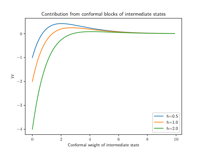
Figure 3: The horizontal axis represents the conformal weight of the intermediate state. We calculated them for the four-point function of identical scalar operators with $h=0.5,1.0,2.0$. We can see that they give negative contributions for the intermediate state with a small conformal weight, and on the other hand, they provide positive contributions above some conformal weight.

5 Conclusions and Discussion

Summary

In this paper, we have done the following:

• We formulated one of the conformal bootstrap equations in momentum space representation at finite volume. We dealt with two-dimensional and three-dimensional CFT, but this approach applies to CFTs with $d>3$.

• In two-dimensional CFT, factorization helps calculate momentum space’s two- and three-point functions. We explained three methods to calculate them, direct integral calculation, algebraic calculation, and WI method, though they are equivalent in principle. The most valuable and fascinating approach is the WI method since this applies to the Wightman function of operators with general conformal weight and the higher-dimensional CFTs.

• On the other hand, three-dimensional CFT is a little tricky to handle. One of the reasons is that the structure of the product of complete orthogonal basis, spherical harmonics $\{Y_{l,m}\}$, in three-dimensional CFT ($S^{2}\times\mathbb{R}$) is more complicated than that, $\{e^{-in\theta}\}$, in two-dimensional CFT ($S^{1}\times\mathbb{R}$). Because of the reason, it was too difficult to find a general solution for WIs. We have to solve the differential equations from (LABEL:ODE1) to (LABEL:ODE6) term by term with the computer.

• Taking large volume limit, we proved that the two-point function and the three-point function we got at finite volume are consistent with the previous result [Gil18, GLLM20, Gil20, Gil21] at infinite volume.

• The main ingredient of this paper is that we explicitly constructed conformal blocks in two-dimensional CFT and showed how we could introduce bootstrap equations in momentum space. We applied the bootstrap equation [GLLM20] obtained from microcausality condition in infinite volume to finite volume case. One of the exciting properties of our formula is that we only have to take a discrete sum because of the quantization of energy and momentum. It helps us calculate conformal blocks analytically and numerically. We proved that our bootstrap equation is not satisfied trivially, which means it could give us a constraint for CFT data.

Remaining challenges

We have some remaining challenges to be solved in the future.

• In two-dimensional CFT, the problem is how, to sum up the contributions from Virasoro descendants. There is no exact result for summing them, so we have to calculate them by computer.

• In three-dimensional CFT, we have technical problems. The most challenging issue to be solved is we do not know the exact form of the three-point functions. We can calculate them term by term with recursion relations obtained from WIs, but it needs calculation by computer. If we could find the exact form, it would make it easier to calculate conformal blocks in three-dimensional CFT.

• In three-dimensional CFT, in this paper, we only dealt with scalar primaries because it is easy to handle. We have to consider various primaries with spin, but we can get them similarly as we did for scalar primaries. The generalization of our result in this paper is one of the remaining challenges, though it is not so hard.

Future research direction

We formulated the basis for the conformal bootstrap equation in momentum space at finite volume. We end our paper with a discussion of future research directions.

• One of the future approaches is to consider better test functions. In this paper, we chose the delta function and step-like function as test functions because they are easy to derive bootstrap equations. In that case, we had to consider many contributions from the intermediate state, whose energy ranges from the lowest one to infinity. If we set a smoother function as a test function, we might get better bootstrap equations in which the contributions from an intermediate state with high energy are suppressed. Considering many types of test functions is one of our future directions.

• This paper dealt with conformal bootstrap obtained from the microcausality condition. In the construction, we ignored the explicit form of the commutator by multiplying the test function that has support only at spacelike region. On the other hand, finding a concrete expression for the commutator is needed to find a valid, closed bootstrap equation for the Wightman function by comparing (43)(21), (42)(31), and (32)(41) channels. However, the commutator of the operators is not well-defined for a non-free CFT, so we need to consider the commutator of the smeared operators for time and space directions. This formulation has been constructed [NT21, BDBM20] but has yet to apply it to the conformal bootstrap equations fully. It is a desirable research direction.

Appendix A Supplement to two-dimensional CFT

A.1 Solution for the Ward Identities

Let us solve ODEs (2.13)-(2.16) obtained from WIs in two-dimensional CFT. Remember that we used $L_{0}$ and $\tilde{L}_{0}$ WIs to determine the reduced form for the two-point function. First, shift $n$ by $n\rightarrow n-s_{1}$, and define $G_{n}\equiv F_{n-s_{1}}$. We get

$$L_{-1} :\left(y\derivative{y}-\Delta_{1}+n-s_{1}+1\right)G_{n+1}(y)+y\left(-y\derivative{y}-\Delta_{2}-n-s_{2}\right)G_{n}(y)=0$$ (A.1)

$$\tilde{L}_{-1} :y\left(-y\derivative{y}-\Delta_{2}+n+1+s_{2}\right)G_{n+1}(y)+\left(y\derivative{y}-\Delta_{1}-n+s_{1}\right)G_{n}(y)=0$$ (A.2)

$$L_{1} :\left(-y\derivative{y}+\Delta_{2}-n-1+s_{2}\right)G_{n+1}(y)+y\left(y\derivative{y}+\Delta_{1}+s_{1}+n\right)G_{n}(y)=0$$ (A.3)

$$\tilde{L}_{1} :y\left(y\derivative{y}+\Delta_{1}-s_{1}-n-1\right)G_{n+1}(y)+\left(-y\derivative{y}+\Delta_{2}+n-s_{2}\right)G_{n}(y)=0.$$ (A.4)

Adding equations (A.1) and (A.3) gives

$$0=2(h_{2}-h_{1})[G_{n+1}(y)-yG_{n}(y)].$$ (A.5)

And adding equations (A.2) and (A.4) gives

$$0=2(\tilde{h}_{1}-\tilde{h}_{2})[yG_{n+1}(y)-G_{n}(y)].$$ (A.6)

There are four possibilities.

$$(1) \ \ \ h_{1}\neq h_{2},\ \tilde{h}_{1}\neq\tilde{h}_{2}\ \ \text{supported only at }y=1$$

$$(2) \ \ \ h_{1}=h_{2},\ G_{n}(y)=y^{-n}G_{0}(y)$$

$$(3) \ \ \ \tilde{h}_{1}=\tilde{h}_{2},\ G_{n}(y)=y^{n}G_{0}(y)$$

$$(4) \ \ \ h_{1}=h_{2},\ \tilde{h}_{1}=\tilde{h}_{2}$$

The first solution is different from what we are looking for. Substituting the second solution for (A.1) gives

$$\derivative{y}G_{0}(y)=2h\frac{1+y^{2}}{y(1-y^{2})}G_{0}(y).$$ (A.7)

Solving them, we get

$$G_{0}(y)\propto\left(\frac{y}{|1-y|(1+y)}\right)^{2h}.$$ (A.8)

So, the Wightman two-point function is

$$C(n_{1},n_{2},r_{1},r_{2})\propto r_{1}^{-\Delta_{1}}r_{2}^{-\Delta_{2}}\delta(n_{1}+n_{2}+s_{1}+s_{2})y^{-n_{1}-s_{1}}\left(\frac{y}{|1-y|(1+y)}\right)^{2h}.$$ (A.9)

The second solution is wrong because it diverges when we take $y$ to $0$ for fixed $r_{2}$. In the same way, we can say that the third solution is wrong. So, we can conclude that $h_{1}=h_{2}\equiv h$ and $\tilde{h}_{1}=\tilde{h}_{2}\equiv\tilde{h}$. Then we only have two independent equations.

$$\left(y\derivative{y}-2h+n+1\right)G_{n+1}(y)+y\left(-y\derivative{y}-2h-n\right)G_{n}(y)=0$$ (A.10)

$$y\left(-y\derivative{y}-2\tilde{h}+n+1\right)G_{n+1}(y)+\left(y\derivative{y}-2\tilde{h}-n\right)G_{n}(y)=0$$ (A.11)

From them, we get

$$G_{n+1} =\frac{1}{2h+2\tilde{h}-2n-2}[(y^{-1}-y)\hat{E}-2hy-2\tilde{h}y^{-1}-(y+y^{-1})n]G_{n}$$ (A.12)

$$G_{n} =\frac{1}{2h+2\tilde{h}+2n}[(y^{-1}-y)\hat{E}-2hy^{-1}-2\tilde{h}y+(y+y^{-1})(n+1)]G_{n+1}.$$ (A.13)

Let us fix $n$ to solve it. The most reasonable choice is $n=s=h-\tilde{h}$.

$$G_{s+1} =\frac{1}{2\Delta-2s-2}[(y^{-1}-y)(\hat{E}+s)-(y^{-1}+y)(\Delta+s)]G_{s}$$ (A.14)

$$G_{s} =\frac{1}{2\Delta+2s}[(y^{-1}-y)(\hat{E}-s)+(y+y^{-1})(s+1-\Delta)]G_{s+1}$$ (A.15)

Combining them gives

$$G^{\prime\prime}_{s}[y]+\frac{(2\Delta+1)y^{2}+(2\Delta-1)}{y^{3}-y}G^{\prime}_{s}[y]+\left(\frac{\Delta^{2}}{y^{2}}+\frac{4s^{2}}{1-y^{2}}\right)G_{s}[y]=0.$$ (A.16)

From unitarity, we can assume that $G_{s}$ must be a discrete sum of the powers of $y$. And small-$y$ behavior of the solution are $G_{s}(y)\propto y^{\Delta}$. From these facts, we get the answer by series expansion.

$$G_{s}[y] =K_{s}y^{\Delta}\sum_{l=0}^{\infty}c_{l}y^{2l}$$ (A.17)

$$c_{l} =\frac{\Gamma(\Delta+s+l)\Gamma(\Delta-s+l)}{\Gamma(\Delta+s)\Gamma(\Delta-s)\Gamma^{2}(l+1)}$$ (A.18)

$K_{s}$ is an undetermined constant depending on the normalization of operators.

Now we get a solution for the primary state with spin $s$. Next, we derive a solution for the excited (descendant) state. The recursion relation is

$$G_{n+s+1}=\frac{1}{2\Delta-2s-2n-2}[(y^{-1}-y)(\hat{E}+s)-(y^{-1}+y)(\Delta+s+n)]G_{n+s}.$$ (A.19)

Assume that the solution has the following form.

$$G_{n+s}=K_{n+s}y^{\Delta+n}\sum_{l\geq 0}b_{n+s|l}y^{2l}=K_{s}y^{\Delta+n}\sum_{l\geq 0}c_{n+s|l}y^{2l}$$ (A.20)

$$K_{n+s}b_{n+s|l}=K_{s}c_{n+s|l}$$ (A.21)

$$b_{s|l}=c_{s|l}=c_{l}=\frac{\Gamma(\Delta+s+l)\Gamma(\Delta-s+l)}{\Gamma(\Delta+s)\Gamma(\Delta-s)\Gamma^{2}(l+1)}$$ (A.22)

$$b_{n+s|l=0}=1$$ (A.23)

We use mathematical induction to get the solution. (1) Calculation of $G_{s+1}$

$$G_{1+s} =K_{1+s}y^{\Delta+1}\sum_{l\geq 0}b_{1+s|l}y^{2l}$$ (A.24)

$$=\frac{1}{2\Delta-2s-2}\left[(1-y^{2})\derivative{y}-y^{-1}\Delta-y(2s+\Delta)\right]K_{s}y^{\Delta}\sum_{l\geq 0}b_{s|l}y^{2l}$$ (A.25)

Picking up the coefficient of $y^{\Delta+1}$ gives

$$K_{1+s}=(\Delta+s)K_{s}.$$ (A.26)

Picking up the coefficient of $y^{\Delta+2l+1}$ gives

$$K_{1+s}b_{1+s|l}=\frac{K_{s}}{l+1}\frac{\Gamma(\Delta+s+l+1)\Gamma(\Delta-s+l)}{\Gamma(\Delta+s)\Gamma(\Delta-s)\Gamma^{2}(l+1)}.$$ (A.27)

So, we get

$$b_{1+s|l} =\frac{\Gamma(\Delta+s+l+1)\Gamma(\Delta-s+l)}{\Gamma(\Delta+s+1)\Gamma(\Delta-s)\Gamma(l+2)\Gamma(l+1)}$$ (A.28)

$$c_{1+s|l} =\frac{K_{1+s}}{K_{s}}b_{1+s|l}=\frac{\Gamma(\Delta+s+l+1)\Gamma(\Delta-s+l)}{\Gamma(\Delta+s)\Gamma(\Delta-s)\Gamma(l+2)\Gamma(l+1)}.$$ (A.29)

(2) Calculation of $G_{s+2}$

$$G_{2+s} =K_{2+s}y^{\Delta+2}\sum_{l\geq 0}b_{2+s|l}y^{2l}$$ (A.30)

$$=\frac{1}{2\Delta-2s-4}\left[(1-y^{2})\derivative{y}-y^{-1}(\Delta+1)-y(2s+\Delta+1)\right]K_{1+s}y^{\Delta+1}\sum_{l\geq 0}b_{1+s|l}y^{2l}$$ (A.31)

Picking up the coefficient of $y^{\Delta+2}$ gives

$$K_{2+s}=\frac{(\Delta+s)(\Delta+s+1)}{2}K_{s}.$$ (A.32)

Picking up the coefficient of $y^{\Delta+2+2l}$ gives

$$b_{2+s|l} =2\frac{\Gamma(\Delta+s+l+2)\Gamma(\Delta-s+l)}{\Gamma(\Delta+s+2)\Gamma(\Delta-s)\Gamma(l+3)\Gamma(l+1)}$$ (A.33)

$$c_{2+s|l} =\frac{K_{2+s}}{K_{s}}b_{2+s|l}=\frac{\Gamma(\Delta+s+l+2)\Gamma(\Delta-s+l)}{\Gamma(\Delta+s)\Gamma(\Delta-s)\Gamma(l+3)\Gamma(l+1)}.$$ (A.34)

(3) General $G_{n+s}$

From (1) and (2), we can guess the form of general $G_{n+s}$.

$$K_{n+s} =\frac{\Gamma(\Delta+s+n)}{\Gamma(n+1)\Gamma(\Delta+s)}K_{s}$$ (A.35)

$$b_{n+s|l} =\frac{\Gamma(1+n)\Gamma(\Delta+s+l+n)\Gamma(\Delta-s+l)}{\Gamma(\Delta+s+n)\Gamma(\Delta-s)\Gamma(l+n+1)\Gamma(l+1)}$$ (A.36)

$$c_{n+s|l} =\frac{\Gamma(\Delta+s+l+n)\Gamma(\Delta-s+l)}{\Gamma(\Delta+s)\Gamma(\Delta-s)\Gamma(l+n+1)\Gamma(l+1)}$$ (A.37)

We show it by mathematical induction. Picking up the coefficient of $y^{\Delta+2+2l}$ gives

$$K_{n+s+1}b_{n+s+1|l}=\frac{K_{n+s}}{\Delta-s-n-1}[(l+1)b_{n+s|l+1}-(l+s+\Delta+n)b_{n+s|l}].$$ (A.38)

From this, we obtain recursion relations for $K_{n+s}$, $b_{n+s|l}$ and $c_{n+s|l}$.

$$K_{n+s+1} =K_{n+s}\frac{b_{n+s|l=1}-(\Delta+s+n)}{\Delta-s-n-1}$$ (A.39)

$$b_{n+s+1|l} =\frac{(l+1)b_{n+s|l+1}-(l+s+\Delta+n)b_{n+s|l}}{b_{n+s|l=1}-(\Delta+s+n)}$$ (A.40)

$$c_{n+s+1} =\frac{K_{n+s+1}}{K_{s}}b_{n+s+1}$$ (A.41)

When the configuration (A.35), (A.36) and (A.37) are valid for $n$,

$$K_{n+s+1}$$

$$=\frac{\Gamma(\Delta+s+n)}{\Gamma(n+1)\Gamma(\Delta+s)}K_{s}\frac{1}{\Delta-s-n-1}\left[\frac{\Gamma(1+n)\Gamma(\Delta+s+1+n)\Gamma(\Delta-s+1)}{\Gamma(\Delta+s+n)\Gamma(\Delta-s)\Gamma(n+2)\Gamma(2)}-(\Delta+s+n)\right]$$

$$=\frac{\Gamma(\Delta+s+n+1)}{\Gamma(n+2)\Gamma(\Delta+s)}K_{s}$$ (A.42)

$$b_{n+s+1|l} =\left[(l+1)\frac{\Gamma(1+n)\Gamma(\Delta+s+l+1+n)\Gamma(\Delta-s+l+1)}{\Gamma(\Delta+s+n)\Gamma(\Delta-s)\Gamma(l+n+2)\Gamma(l+2)}-\right.$$

$$\left.\hskip 85.35826pt(l+s+\Delta+n)\frac{\Gamma(1+n)\Gamma(\Delta+s+l+n)\Gamma(\Delta-s+l)}{\Gamma(\Delta+s+n)\Gamma(\Delta-s)\Gamma(l+n+1)\Gamma(l+1)}\right]$$

$$\hskip 14.22636pt\left[\frac{\Gamma(1+n)\Gamma(\Delta+s+1+n)\Gamma(\Delta-s+1)}{\Gamma(\Delta+s+n)\Gamma(\Delta-s)\Gamma(n+2)\Gamma(2)}-(\Delta+s+n)\right]^{-1}$$

$$=\frac{\Gamma(2+n)\Gamma(\Delta+s+l+n)\Gamma(\Delta-s+l)}{\Gamma(\Delta+s+n)\Gamma(\Delta-s)\Gamma(l+n+2)\Gamma(l+2)}\frac{(l+1)(\Delta+s+l+n)(\Delta-s-n-1)}{(\Delta+s+n)(\Delta-s-n-1)}$$

$$=\frac{\Gamma(2+n)\Gamma(\Delta+s+l+n+1)\Gamma(\Delta-s+l)}{\Gamma(\Delta+s+n+1)\Gamma(\Delta-s)\Gamma(l+n+2)\Gamma(l+1)}$$ (A.43)

$$c_{n+s+1|l} =\frac{\Gamma(\Delta+s+n+1)}{\Gamma(n+2)\Gamma(\Delta+s)}\frac{\Gamma(2+n)\Gamma(\Delta+s+l+n+1)\Gamma(\Delta-s+l)}{\Gamma(\Delta+s+n+1)\Gamma(\Delta-s)\Gamma(l+n+2)\Gamma(l+1)}$$

$$=\frac{\Gamma(\Delta+s+l+n+1)\Gamma(\Delta-s+l)}{\Gamma(\Delta+s)\Gamma(\Delta-s)\Gamma(l+n+2)\Gamma(l+1)}.$$ (A.44)

So, the configurations (A.35), (A.36) and (A.37) are also valid for $n+1$. By mathematical induction, we get (A.35), (A.36) and (A.37) for positive integer $n$. In the same way, we can also get the solution for negative $n$.

A.2 Direct integral calculation of three-point function

Let us perform the Fourier transform directly for the three-point function.

$$\langle\mathcal{O}_{n_{3}}(r_{3})\mathcal{O}_{n_{2}}(r_{2})\mathcal{O}_{n_{1}}(r_{1})\rangle=\frac{1}{(2\pi i)^{3}}\oint\frac{dz_{3}}{z_{3}^{1+n_{3}}}\oint\frac{dz_{2}}{z_{2}^{1+n_{2}}}\oint\frac{dz_{1}}{z_{1}^{1+n_{1}}}\lambda_{321}z_{21}^{-b_{3}}z_{32}^{-b_{1}}z_{31}^{-b_{2}}$$ (A.45)

First, integrate it with respect to $z_{1}$.

$$\frac{\lambda_{321}}{2\pi i}\oint\frac{dz_{1}}{z_{1}^{1+n_{1}}}z_{21}^{-b_{3}}z_{32}^{-b_{1}}z_{31}^{-b_{2}}=\frac{\lambda_{321}}{\Gamma(b_{3})\Gamma(b_{2})}\sum_{k=0}^{n_{1}}\frac{\Gamma(b_{3}+k)\Gamma(b_{2}+n_{1}-k)}{\Gamma(1+k)\Gamma(1+n_{1}-k)}z_{2}^{-b_{3}-k}z_{3}^{-b_{2}-n_{1}+k}z_{32}^{-b_{1}}$$ (A.46)

Next, define $\omega_{3}=1/z_{3}$ and integrate it with respect to $\omega_{3}$. Under this transformation, the contour integral around $z=\infty$ becomes contour integral around $\omega_{3}=0$.

$$\frac{1}{2\pi i}\oint\frac{dz_{3}}{z_{3}^{1+n_{3}}}\text{(\ref{integral1})}=\frac{1}{2\pi i}\oint\frac{d\omega_{3}}{\omega_{3}^{1+m_{3}}}\frac{\lambda_{321}}{\Gamma(b_{3})\Gamma(b_{2})}\sum_{k=0}^{n_{1}}\frac{\Gamma(b_{3}+k)\Gamma(b_{2}+n_{1}-k)}{\Gamma(1+k)\Gamma(1+n_{1}-k)}\frac{z_{2}^{-b_{3}-k}\omega_{3}^{n_{1}-k}}{(1-z_{2}\omega_{3})^{b_{1}}}$$ (A.47)

Here, we defined $m_{3}\equiv-n_{3}-2h_{3}$. There are two cases. $m_{3}\geq n_{1}$ or $m_{3}\leq n_{1}$. (1) $m_{3}\leq n_{1}$

$$\text{(\ref{integral2})}=\frac{\lambda_{123}}{\Gamma(b_{3})\Gamma(b_{2})}\sum_{k=n_{1}-m_{3}}^{n_{1}}\frac{\Gamma(b_{3}+k)\Gamma(b_{2}+n_{1}-k)}{\Gamma(1+k)\Gamma(1+n_{1}-k)}\frac{\Gamma(b_{1}+m_{3}-n_{1}+k)}{\Gamma(m_{3}-n_{1}+k+1)\Gamma(b_{1})}z_{2}^{-b_{3}+m_{3}-n_{1}}$$ (A.48)

So, the three-point function is

$$\text{(\ref{integral0})}=\frac{\delta\left(\sum_{i=1}^{3}(n_{i}+h_{i})\right)\lambda_{123}}{\Gamma(b_{3})\Gamma(b_{2})\Gamma(b_{1})}\sum_{k=n_{1}-m_{3}}^{n_{1}}\frac{\Gamma(b_{3}+k)\Gamma(b_{2}+n_{1}-k)}{\Gamma(1+k)\Gamma(1+n_{1}-k)}\frac{\Gamma(b_{1}+m_{3}-n_{1}+k)}{\Gamma(1+m_{3}-n_{1}+k)}.$$ (A.49)

(2) $m_{3}\geq n_{1}$

$$\text{(\ref{integral2})}=\frac{\lambda_{123}}{\Gamma(b_{3})\Gamma(b_{2})}\sum_{k=0}^{n_{1}}\frac{\Gamma(b_{3}+k)\Gamma(b_{2}+n_{1}-k)}{\Gamma(1+k)\Gamma(1+n_{1}-k)}\frac{\Gamma(b_{1}+m_{3}-n_{1}+k)}{\Gamma(m_{3}-n_{1}+k+1)\Gamma(b_{1})}z_{2}^{-b_{3}+m_{3}-n_{1}}$$ (A.50)

So, the three-point function is

$$\text{(\ref{integral0})}=\frac{\delta\left(\sum_{i=1}^{3}(n_{i}+h_{i})\right)\lambda_{123}}{\Gamma(b_{3})\Gamma(b_{2})\Gamma(b_{1})}\sum_{k=0}^{n_{1}}\frac{\Gamma(b_{3}+k)\Gamma(b_{2}+n_{1}-k)}{\Gamma(1+k)\Gamma(1+n_{1}-k)}\frac{\Gamma(b_{1}+m_{3}-n_{1}+k)}{\Gamma(1+m_{3}-n_{1}+k)}.$$ (A.51)

In the end, we get

$$\text{(\ref{integral0})}=\frac{\delta\left(\sum_{i=1}^{3}(n_{i}+h_{i})\right)\lambda_{123}}{\Gamma(b_{3})\Gamma(b_{2})\Gamma(b_{1})}\sum_{k=\rm{Max}\{0,n_{1}-m_{3}\}}^{n_{1}}\frac{\Gamma(b_{3}+k)\Gamma(b_{2}+n_{1}-k)}{\Gamma(1+k)\Gamma(1+n_{1}-k)}\frac{\Gamma(b_{1}+m_{3}-n_{1}+k)}{\Gamma(1+m_{3}-n_{1}+k)}.$$ (A.52)

Define a new variable $q\equiv k-\mathrm{Max}\{0,n_{1}-m_{3}\}$. Then, we get

$$\langle\mathcal{O}_{n_{3}}(r_{3})\mathcal{O}_{n_{2}}(r_{2})\mathcal{O}_{n_{1}}(r_{1})\rangle=\delta(n_{1}+n_{2}+n_{3}+h_{1}+h_{2}+h_{3})\frac{\lambda_{321}}{\Gamma(b_{1})\Gamma(b_{2})\Gamma(b_{3})}$$ (A.53)

$$\sum_{q=0}^{\mathrm{Min}\{n_{1},m_{3}\}}\frac{\Gamma[b_{3}+q+\mathrm{Max}\{{0,n_{1}-m_{3}}\}]\Gamma[b_{2}-q+\mathrm{Min}\{{n_{1},m_{3}}\}]\Gamma[b_{1}+q+\mathrm{Max}\{{m_{3}-n_{1},0}\}]}{\Gamma[1+q+\mathrm{Max}\{{0,n_{1}-m_{3}}\}]\Gamma[1-q+\mathrm{Min}\{{n_{1},m_{3}}\}]\Gamma[1+q+\mathrm{Max}\{{m_{3}-n_{1},0}\}]}$$

It is valid for all integer $n_{1}$ and $m_{3}$, and invariant under the time-reversal transformation ($n_{1}\Leftrightarrow m_{3}$, $b_{1}\Leftrightarrow b_{3}$).

A.3 Consistency check for three-point function

A.3.1 Ward Identities for three-point function

Define the complete Wightman three-point function as

$$C(n_{1},n_{2},n_{3},r_{1},r_{2},r_{3})\equiv\langle\mathcal{\tilde{O}}^{(3)}_{n_{3}}(r_{3})\mathcal{\tilde{O}}^{(2)}_{n_{2}}(r_{2})\mathcal{\tilde{O}}^{(1)}_{n_{1}}(r_{1})\rangle.$$ (A.54)

We get a reduced three-point function using $L_{0}\pm\tilde{L}_{0}$ WIs.

$$C(n_{1},n_{2},n_{3})=r_{1}^{-\Delta_{1}}r_{2}^{-\Delta_{2}}r_{3}^{-\Delta_{3}}\delta(n_{1}+n_{2}+n_{3}+s_{1}+s_{2}+s_{3})F(n_{1},n_{3},y_{1},y_{3})$$ (A.55)

with $y_{1}\equiv\frac{r_{1}}{r_{2}}$ and $y_{3}\equiv\frac{r_{3}}{r_{2}}$. Next, consider $P_{z},\ P_{\bar{z}},\ K^{z}$ and $K^{\bar{z}}$ WIs.

$$P_{z}\cdot C(n_{1},n_{2},n_{3})=0$$

$$=\frac{1}{2r_{3}}\left(r_{3}\derivative{r_{3}}+n_{3}+1\right)C(n_{1},n_{2},n_{3}+1)+\frac{1}{2r_{2}}\left(r_{2}\derivative{r_{2}}+n_{2}+1\right)C(n_{1},n_{2}+1,n_{3})$$

$$\ \ \ \ \ \ \ \ \ \ \ \ +\frac{1}{2r_{1}}\left(r_{1}\derivative{r_{1}}+n_{1}+1\right)C(n_{1}+1,n_{2},n_{3})$$ (A.56)

$$K^{z}\cdot C(n_{1},n_{2},n_{3})=0$$

$$=\frac{r_{3}}{2}\left(r_{3}\derivative{r_{3}}+n_{3}+4h_{3}-1\right)C(n_{1},n_{2},n_{3}-1)+\frac{r_{2}}{2}\left(r_{2}\derivative{r_{2}}+n_{2}+4h_{2}-1\right)C(n_{1},n_{2}-1,n_{3})$$

$$\ \ \ \ \ \ \ \ \ \ \ \ +\frac{r_{1}}{2}\left(r_{1}\derivative{r_{1}}+n_{1}+4h_{1}-1\right)C(n_{1}-1,n_{2},n_{3})$$ (A.57)

$$P_{\bar{z}}\cdot C(n_{1},n_{2},n_{3})=0$$

$$=\frac{1}{2r_{3}}\left(r_{3}\derivative{r_{3}}-n_{3}+1\right)C(n_{1},n_{2},n_{3}-1)+\frac{1}{2r_{2}}\left(r_{2}\derivative{r_{2}}-n_{2}+1\right)C(n_{1},n_{2}-1,n_{3})$$

$$\ \ \ \ \ \ \ \ \ \ \ \ +\frac{1}{2r_{1}}\left(r_{1}\derivative{r_{1}}-n_{1}+1\right)C(n_{1}-1,n_{2},n_{3})$$ (A.58)

$$K^{\bar{z}}\cdot C(n_{1},n_{2},n_{3})=0$$

$$=\frac{r_{3}}{2}\left(r_{3}\derivative{r_{3}}-n_{3}+4\tilde{h}_{3}-1\right)C(n_{1},n_{2},n_{3}+1)+\frac{r_{2}}{2}\left(r_{2}\derivative{r_{2}}-n_{2}+4\tilde{h}_{2}-1\right)C(n_{1},n_{2}+1,n_{3})$$

$$\ \ \ \ \ \ \ \ \ \ \ \ +\frac{r_{1}}{2}\left(r_{1}\derivative{r_{1}}-n_{1}+4\tilde{h}_{1}-1\right)C(n_{1}+1,n_{2},n_{3})$$ (A.59)

Substitute the reduced form for WIs. We get

$$\mathrm{P_{z}\ Ward\ Identity}:\ \ \ \ \ 0= \frac{1}{y_{3}}\left(y_{3}\derivative{y_{3}}+n_{3}-\Delta_{3}+1\right)F(n_{1},n_{3}+1,y_{1},y_{3})$$

$$+\left(-y_{1}\derivative{y_{1}}-y_{3}\derivative{y_{3}}-n_{1}-n_{3}-s_{1}-s_{3}-2h_{2}\right)F(n_{1},n_{3},y_{1},y_{3})$$

$$+\frac{1}{y_{1}}\left(y_{1}\derivative{y_{1}}+n_{1}-\Delta_{1}+1\right)F(n_{1}+1,n_{3},y_{1},y_{3})$$ (A.60)

$$\mathrm{P_{\bar{z}}\ Ward\ Identity}:\ \ \ \ \ 0= \frac{1}{y_{3}}\left(y_{3}\derivative{y_{3}}-n_{3}-\Delta_{3}+1\right)F(n_{1},n_{3}-1,y_{1},y_{3})$$

$$+\left(-y_{1}\derivative{y_{1}}-y_{3}\derivative{y_{3}}+n_{1}+n_{3}+s_{1}+s_{3}-2\tilde{h}_{2}\right)F(n_{1},n_{3},y_{1},y_{3})$$

$$+\frac{1}{y_{1}}\left(y_{1}\derivative{y_{1}}-n_{1}-\Delta_{1}+1\right)F(n_{1}-1,n_{3},y_{1},y_{3})$$ (A.61)

$$\mathrm{K^{z}\ Ward\ Identity}:\ \ \ \ \ 0= y_{3}\left(y_{3}\derivative{y_{3}}+n_{3}+4h_{3}-\Delta_{3}-1\right)F(n_{1},n_{3}-1,y_{1},y_{3})$$

$$+\left(-y_{1}\derivative{y_{1}}-y_{3}\derivative{y_{3}}-n_{1}-n_{3}-s_{1}-s_{3}+2h_{2}\right)F(n_{1},n_{3},y_{1},y_{3})$$

$$+y_{1}\left(y_{1}\derivative{y_{1}}+n_{1}+4h_{1}-\Delta_{1}-1\right)F(n_{1}-1,n_{3},y_{1},y_{3})$$ (A.62)

$$\mathrm{K^{\bar{z}}\ Ward\ Identity}:\ \ \ \ \ 0= y_{3}\left(y_{3}\derivative{y_{3}}-n_{3}+4\tilde{h}_{3}-\Delta_{3}-1\right)F(n_{1},n_{3}+1,y_{1},y_{3})$$

$$+\left(-y_{1}\derivative{y_{1}}-y_{3}\derivative{y_{3}}+n_{1}+n_{3}+s_{1}+s_{3}+2\tilde{h}_{2}\right)F(n_{1},n_{3},y_{1},y_{3})$$

$$+y_{1}\left(y_{1}\derivative{y_{1}}-n_{1}+4\tilde{h}_{1}-\Delta_{1}-1\right)F(n_{1}+1,n_{3},y_{1},y_{3}).$$ (A.63)

A.3.2 Reduction of Ward Identities for holomorphic three-point function

The relation between $\mathcal{K}_{\mathrm{red}}(n_{1},m_{3})$ and $F(n_{1},n_{3},y_{1},y_{3})$ is

$$\mathcal{K}_{\mathrm{red}}(n_{1},m_{3})r_{1}^{n_{1}}r_{2}^{n_{2}}r_{3}^{n_{3}}=r_{1}^{-\Delta_{1}}r_{2}^{-\Delta_{2}}r_{3}^{-\Delta_{3}}F(n_{1},n_{3},y_{1},y_{3}).$$ (A.64)

Remember that $m_{3}$ is defined as $m_{3}=-(n_{3}+2h_{3})$. Then,

$$F(n_{1},n_{3},y_{1},y_{3})=y_{1}^{n_{1}+h_{1}}y_{3}^{n_{3}+h_{3}}\mathcal{K}_{\mathrm{red}}(n_{1},m_{3}).$$ (A.65)

For holomorphic operators, WIs for $F(n_{1},n_{3},y_{1},y_{3})$ are

$$\mathrm{P_{z}\ Ward\ Identity}:\ \ \ \ \ 0= \frac{1}{y_{3}}\left(y_{3}\derivative{y_{3}}+n_{3}-h_{3}+1\right)F(n_{1},n_{3}+1,y_{1},y_{3})$$

$$+\left(-y_{1}\derivative{y_{1}}-y_{3}\derivative{y_{3}}-n_{1}-n_{3}-h_{1}-h_{3}-2h_{2}\right)F(n_{1},n_{3},y_{1},y_{3})$$

$$+\frac{1}{y_{1}}\left(y_{1}\derivative{y_{1}}+n_{1}-h_{1}+1\right)F(n_{1}+1,n_{3},y_{1},y_{3})$$ (A.66)

$$\mathrm{P_{\bar{z}}\ Ward\ Identity}:\ \ \ \ \ 0= \frac{1}{y_{3}}\left(y_{3}\derivative{y_{3}}-n_{3}-h_{3}+1\right)F(n_{1},n_{3}-1,y_{1},y_{3})$$

$$+\left(-y_{1}\derivative{y_{1}}-y_{3}\derivative{y_{3}}+n_{1}+n_{3}+h_{1}+h_{3}\right)F(n_{1},n_{3},y_{1},y_{3})$$

$$+\frac{1}{y_{1}}\left(y_{1}\derivative{y_{1}}-n_{1}-h_{1}+1\right)F(n_{1}-1,n_{3},y_{1},y_{3})$$ (A.67)

$$\mathrm{K^{z}\ Ward\ Identity}:\ \ \ \ \ 0= y_{3}\left(y_{3}\derivative{y_{3}}+n_{3}+3h_{3}-1\right)F(n_{1},n_{3}-1,y_{1},y_{3})$$

$$+\left(-y_{1}\derivative{y_{1}}-y_{3}\derivative{y_{3}}-n_{1}-n_{3}-h_{1}-h_{3}+2h_{2}\right)F(n_{1},n_{3},y_{1},y_{3})$$

$$+y_{1}\left(y_{1}\derivative{y_{1}}+n_{1}+3h_{1}-1\right)F(n_{1}-1,n_{3},y_{1},y_{3})$$ (A.68)

$$\mathrm{K^{\bar{z}}\ Ward\ Identity}:\ \ \ \ \ 0= y_{3}\left(y_{3}\derivative{y_{3}}-n_{3}-h_{3}-1\right)F(n_{1},n_{3}+1,y_{1},y_{3})$$

$$+\left(-y_{1}\derivative{y_{1}}-y_{3}\derivative{y_{3}}+n_{1}+n_{3}+h_{1}+h_{3}\right)F(n_{1},n_{3},y_{1},y_{3})$$

$$+y_{1}\left(y_{1}\derivative{y_{1}}-n_{1}-h_{1}-1\right)F(n_{1}+1,n_{3},y_{1},y_{3}).$$ (A.69)

Substituting (A.65) for them gives the following relations.

$$P_{z} :0=(n_{3}+1)\mathcal{K}_{\mathrm{red}}(n_{1},n_{3}+1)-(h_{1}+h_{2}+h_{3}+n_{1}+n_{3})\mathcal{K}_{\mathrm{red}}(n_{1},n_{3})$$

$$\hskip 28.45274pt+(n_{1}+1)\mathcal{K}_{\mathrm{red}}(n_{1}+1,n_{3})$$ (A.70)

$$P_{\bar{z}} :\mathrm{satisfied\ trivially}$$

$$K^{z} :0=(n_{3}+2h_{3}-1)\mathcal{K}_{\mathrm{red}}(n_{1},n_{3}-1)-(n_{1}+n_{3}+h_{1}+h_{3}-h_{2})\mathcal{K}_{\mathrm{red}}(n_{1},n_{3})$$

$$\hskip 28.45274pt+(n_{1}+2h_{1}-1)\mathcal{K}_{\mathrm{red}}(n_{1}-1,n_{3})$$ (A.71)

$$K^{\bar{z}} :\mathrm{satisfied\ trivially}$$

They are the reduced WIs for the holomorphic three-point function. All we have to do is to check whether this $P_{z}$ WI and $K^{z}$ WI are satisfied.

A.3.3 Consistency check

We have to prove the following equations. For reduced $P_{z}$ WI, we get

$$0 =(n_{3}+1)\sum_{k=\mathrm{MAX}\{0,n_{1}-m_{3}+1\}}^{n_{1}}\frac{\Gamma(b_{3}+k)\Gamma(b_{2}+n_{1}-k)\Gamma(b_{1}+m_{3}-n_{1}+k-1)}{\Gamma(1+k)\Gamma(1+n_{1}-k)\Gamma(1+m_{3}-n_{1}+k-1)}$$

$$\ -(n_{1}+n_{3}+h_{1}+h_{2}+h_{3})\sum_{k=\mathrm{MAX}\{0,n_{1}-m_{3}\}}^{n_{1}}\frac{\Gamma(b_{3}+k)\Gamma(b_{2}+n_{1}-k)\Gamma(b_{1}+m_{3}-n_{1}+k)}{\Gamma(1+k)\Gamma(1+n_{1}-k)\Gamma(1+m_{3}-n_{1}+k)}$$

$$\ +(n_{1}+1)\sum_{k=\mathrm{MAX}\{0,n_{1}-m_{3}+1\}}^{n_{1}+1}\frac{\Gamma(b_{3}+k)\Gamma(b_{2}+n_{1}+1-k)\Gamma(b_{1}+m_{3}-n_{1}+k-1)}{\Gamma(1+k)\Gamma(1+n_{1}+1-k)\Gamma(1+m_{3}-n_{1}+k-1)}.$$ (A.72)

For reduced $K^{z}$ WI, we get

$$0 =(2h_{3}+n_{3}-1)\sum_{k=\mathrm{MAX}\{0,n_{1}-1-m_{3}\}}^{n_{1}}\frac{\Gamma(b_{3}+k)\Gamma(b_{2}+n_{1}-k)\Gamma(b_{1}+m_{3}-n_{1}+k+1)}{\Gamma(1+k)\Gamma(1+n_{1}-k)\Gamma(1+m_{3}-n_{1}+k+1)}$$

$$-(h_{1}-h_{2}+h_{3}+n_{1}+n_{3})\sum_{k=\mathrm{MAX}\{0,n_{1}-m_{3}\}}^{n_{1}}\frac{\Gamma(b_{3}+k)\Gamma(b_{2}+n_{1}-k)\Gamma(b_{1}+m_{3}-n_{1}+k)}{\Gamma(1+k)\Gamma(1+n_{1}-k)\Gamma(1+m_{3}-n_{1}+k)}$$

$$+(2h_{1}+n_{1}-1)\sum_{k=\mathrm{MAX}\{0,n_{1}-1-m_{3}\}}^{n_{1}-1}\frac{\Gamma(b_{3}+k)\Gamma(b_{2}+n_{1}-1-k)\Gamma(b_{1}+m_{3}-n_{1}+k+1)}{\Gamma(1+k)\Gamma(1+n_{1}-1-k)\Gamma(1+m_{3}-n_{1}+k+1)}.$$ (A.73)

(A-1) $P_{z}$ WI for $n_{1}+1\leq m_{3}$

When $n_{1}+1\leq m_{3}$, RHS of (A.72) is

$$\mathrm{(RHS)} =(-m_{3}-b_{1}-b_{2}+1)\sum_{k=0}^{n_{1}}\frac{\Gamma(b_{3}+k)\Gamma(b_{2}+n_{1}-k)\Gamma(b_{1}+m_{3}-n_{1}+k-1)}{\Gamma(1+k)\Gamma(1+n_{1}-k)\Gamma(1+m_{3}-n_{1}+k-1)}$$

$$\ -(n_{1}-m_{3}+b_{3})\sum_{k=0}^{n_{1}}\frac{\Gamma(b_{3}+k)\Gamma(b_{2}+n_{1}-k)\Gamma(b_{1}+m_{3}-n_{1}+k)}{\Gamma(1+k)\Gamma(1+n_{1}-k)\Gamma(1+m_{3}-n_{1}+k)}$$

$$\ +(n_{1}+1)\sum_{k=0}^{n_{1}+1}\frac{\Gamma(b_{3}+k)\Gamma(b_{2}+n_{1}+1-k)\Gamma(b_{1}+m_{3}-n_{1}+k-1)}{\Gamma(1+k)\Gamma(1+n_{1}+1-k)\Gamma(1+m_{3}-n_{1}+k-1)}.$$ (A.74)

We call the first term (A), the second term (B), and the third term (C).

$$\mathrm{(A)} =(-m_{3}-b_{1}-b_{2}+1)\sum_{k=0}^{n_{1}}\frac{\Gamma(b_{3}+k)\Gamma(b_{2}+n_{1}-k)\Gamma(b_{1}+m_{3}-n_{1}+k-1)}{\Gamma(1+k)\Gamma(1+n_{1}-k)\Gamma(1+m_{3}-n_{1}+k-1)}$$

$$\mathrm{(B)} =-(n_{1}-m_{3}+b_{3})\sum_{k=0}^{n_{1}}\frac{\Gamma(b_{3}+k)\Gamma(b_{2}+n_{1}-k)\Gamma(b_{1}+m_{3}-n_{1}+k)}{\Gamma(1+k)\Gamma(1+n_{1}-k)\Gamma(1+m_{3}-n_{1}+k)}$$

$$\mathrm{(C)} =(n_{1}+1)\sum_{k=0}^{n_{1}+1}\frac{\Gamma(b_{3}+k)\Gamma(b_{2}+n_{1}+1-k)\Gamma(b_{1}+m_{3}-n_{1}+k-1)}{\Gamma(1+k)\Gamma(1+n_{1}+1-k)\Gamma(1+m_{3}-n_{1}+k-1)}$$ (A.75)

Then, we get

$$\mathrm{(A)} =-\sum_{k=0}^{n_{1}}(b_{1}+b_{2}+m_{3}-1)\frac{\Gamma(b_{3}+k)\Gamma(b_{2}+n_{1}-k)\Gamma(b_{1}+m_{3}-n_{1}+k-1)}{\Gamma(1+k)\Gamma(1+n_{1}-k)\Gamma(1+m_{3}-n_{1}+k-1)}$$

$$=-\sum_{k=0}^{n_{1}}(m_{3}-n_{1}+k)\frac{\Gamma(b_{3}+k)\Gamma(b_{2}+n_{1}-k)\Gamma(b_{1}+m_{3}-n_{1}+k)}{\Gamma(1+k)\Gamma(1+n_{1}-k)\Gamma(m_{3}-n_{1}+k+1)}$$

$$\ \ \ \ \ -\sum_{k=0}^{n_{1}}(1+n_{1}-k)\frac{\Gamma(b_{3}+k)\Gamma(b_{2}+n_{1}-k+1)\Gamma(b_{1}+m_{3}-n_{1}+k-1)}{\Gamma(1+k)\Gamma(2+n_{1}-k)\Gamma(m_{3}-n_{1}+k)}.$$

We call the first term (A-1) and the second (A-2). Then, we get

$$\mathrm{(RHS)}=\mathrm{((A-1)}+\mathrm{(B))}+\mathrm{((A-2)}+\mathrm{(C))}$$

$$=\frac{\Gamma(b_{3}+n_{1}+1)\Gamma(b_{2})\Gamma(b_{1}+m_{3})}{\Gamma(1+n_{1})\Gamma(1)\Gamma(1+m_{3})}+\sum_{k=0}^{n_{1}}\frac{\Gamma(b_{3}+k)\Gamma(b_{2}+n_{1}-k+1)\Gamma(b_{1}+m_{3}-n_{1}+k-1)}{\Gamma(k)\Gamma(2+n_{1}-k)\Gamma(m_{3}-n_{1}+k)}$$

$$\ \ \ \ \ -\sum_{k=0}^{n_{1}}(b_{3}+k)\frac{\Gamma(b_{3}+k)\Gamma(b_{2}+n_{1}-k)\Gamma(b_{1}+m_{3}-n_{1}+k)}{\Gamma(1+k)\Gamma(1+n_{1}-k)\Gamma(m_{3}-n_{1}+k+1)}$$

$$=\frac{\Gamma(b_{3}+n_{1}+1)\Gamma(b_{2})\Gamma(b_{1}+m_{3})}{\Gamma(1+n_{1})\Gamma(1)\Gamma(1+m_{3})}+\sum_{k=1}^{n_{1}}\frac{\Gamma(b_{3}+k)\Gamma(b_{2}+n_{1}-k+1)\Gamma(b_{1}+m_{3}-n_{1}+k-1)}{\Gamma(k)\Gamma(2+n_{1}-k)\Gamma(m_{3}-n_{1}+k)}$$

$$\ \ \ \ \ -\sum_{k=1}^{n_{1}+1}\frac{\Gamma(b_{3}+k)\Gamma(b_{2}+n_{1}-k+1)\Gamma(b_{1}+m_{3}-n_{1}+k-1)}{\Gamma(k)\Gamma(2+n_{1}-k)\Gamma(m_{3}-n_{1}+k)}$$

$$=\frac{\Gamma(b_{3}+n_{1}+1)\Gamma(b_{2})\Gamma(b_{1}+m_{3})}{\Gamma(1+n_{1})\Gamma(1)\Gamma(1+m_{3})}-\frac{\Gamma(b_{3}+n_{1}+1)\Gamma(b_{2})\Gamma(b_{1}+m_{3})}{\Gamma(1+n_{1})\Gamma(1)\Gamma(1+m_{3})}$$

$$=0.$$ (A.77)

The above calculation shows that $P_{z}$ WI is satisfied for $n_{1}+1\leq m_{3}$. (A-2) $P_{z}$ WI for $n_{1}\geq m_{3}$ When $n_{1}\geq m_{3}$, RHS of (A.72) is

$$\mathrm{(RHS)} =(-m_{3}-b_{1}-b_{2}+1)\sum_{k=n_{1}-m_{3}+1}^{n_{1}}\frac{\Gamma(b_{3}+k)\Gamma(b_{2}+n_{1}-k)\Gamma(b_{1}+m_{3}-n_{1}+k-1)}{\Gamma(1+k)\Gamma(1+n_{1}-k)\Gamma(1+m_{3}-n_{1}+k-1)}$$

$$\ -(n_{1}-m_{3}+b_{3})\sum_{k=n_{1}-m_{3}}^{n_{1}}\frac{\Gamma(b_{3}+k)\Gamma(b_{2}+n_{1}-k)\Gamma(b_{1}+m_{3}-n_{1}+k)}{\Gamma(1+k)\Gamma(1+n_{1}-k)\Gamma(1+m_{3}-n_{1}+k)}$$

$$\ +(n_{1}+1)\sum_{k=n_{1}-m_{3}+1}^{n_{1}+1}\frac{\Gamma(b_{3}+k)\Gamma(b_{2}+n_{1}+1-k)\Gamma(b_{1}+m_{3}-n_{1}+k-1)}{\Gamma(1+k)\Gamma(1+n_{1}+1-k)\Gamma(1+m_{3}-n_{1}+k-1)}.$$ (A.78)

We call the first term (D), the second term (E), and the third term (F).

$$\mathrm{(D)} =(-m_{3}-b_{1}-b_{2}+1)\sum_{k=n_{1}-m_{3}+1}^{n_{1}}\frac{\Gamma(b_{3}+k)\Gamma(b_{2}+n_{1}-k)\Gamma(b_{1}+m_{3}-n_{1}+k-1)}{\Gamma(1+k)\Gamma(1+n_{1}-k)\Gamma(1+m_{3}-n_{1}+k-1)}$$

$$\mathrm{(E)} =-(n_{1}-m_{3}+b_{3})\sum_{k=n_{1}-m_{3}}^{n_{1}}\frac{\Gamma(b_{3}+k)\Gamma(b_{2}+n_{1}-k)\Gamma(b_{1}+m_{3}-n_{1}+k)}{\Gamma(1+k)\Gamma(1+n_{1}-k)\Gamma(1+m_{3}-n_{1}+k)}$$

$$\mathrm{(F)} =(n_{1}+1)\sum_{k=n_{1}-m_{3}+1}^{n_{1}+1}\frac{\Gamma(b_{3}+k)\Gamma(b_{2}+n_{1}+1-k)\Gamma(b_{1}+m_{3}-n_{1}+k-1)}{\Gamma(1+k)\Gamma(1+n_{1}+1-k)\Gamma(1+m_{3}-n_{1}+k-1)}$$ (A.79)

Then, we get

$$\mathrm{(D)} =-\sum_{k=n_{1}-m_{3}+1}^{n_{1}}(m_{3}+b_{1}+b_{2}-1)\frac{\Gamma(b_{3}+k)\Gamma(b_{2}+n_{1}-k)\Gamma(b_{1}+m_{3}-n_{1}+k-1)}{\Gamma(1+k)\Gamma(1+n_{1}-k)\Gamma(1+m_{3}-n_{1}+k-1)}$$

$$=-\sum_{k=n_{1}-m_{3}+1}^{n_{1}}(m_{3}-n_{1}+k)\frac{\Gamma(b_{3}+k)\Gamma(b_{2}+n_{1}-k)\Gamma(b_{1}+m_{3}-n_{1}+k)}{\Gamma(1+k)\Gamma(1+n_{1}-k)\Gamma(1+m_{3}-n_{1}+k)}$$

$$\hskip 28.45274pt-\sum_{k=n_{1}-m_{3}+1}^{n_{1}}(1+n_{1}-k)\frac{\Gamma(b_{3}+k)\Gamma(b_{2}+n_{1}-k+1)\Gamma(b_{1}+m_{3}-n_{1}+k-1)}{\Gamma(1+k)\Gamma(1+n_{1}-k+1)\Gamma(1+m_{3}-n_{1}+k-1)}.$$ (A.80)

We call the first term (D-1) and the second (D-2). Then, we get

$$\mathrm{(RHS)}=\mathrm{((D-1)}+\mathrm{(E))}+\mathrm{((D-2)}+\mathrm{(F))}$$

$$=-(n_{1}-m_{3}+b_{3})\frac{\Gamma(b_{3}+n_{1}-m_{3})\Gamma(b_{2}+m_{3})\Gamma(b_{1})}{\Gamma(1+n_{1}-m_{3})\Gamma(1+m_{3})\Gamma(1)}$$

$$\hskip 28.45274pt-\sum_{k=n_{1}-m_{3}+1}^{n_{1}}(b_{3}+k)\frac{\Gamma(b_{3}+k)\Gamma(b_{2}+n_{1}-k)\Gamma(b_{1}+m_{3}-n_{1}+k)}{\Gamma(1+k)\Gamma(1+n_{1}-k)\Gamma(1+m_{3}-n_{1}+k)}$$

$$+(n_{1}+1)\frac{\Gamma(b_{3}+n_{1}+1)\Gamma(b_{2})\Gamma(b_{1}+m_{3})}{\Gamma(1+n_{1}+1)\Gamma(1)\Gamma(1+m_{3})}$$

$$\hskip 28.45274pt+\sum_{k=n_{1}-m_{3}}^{n_{1}-1}(b_{3}+k)\frac{\Gamma(b_{3}+k)\Gamma(b_{2}+n_{1}-k)\Gamma(b_{1}+m_{3}-n_{1}+k)}{\Gamma(1+k)\Gamma(1+n_{1}-k)\Gamma(1+m_{3}-n_{1}+k)}$$

$$=-\frac{\Gamma(b_{3}+n_{1}-m_{3}+1)\Gamma(b_{2}+m_{3})\Gamma(b_{1})}{\Gamma(1+n_{1}-m_{3})\Gamma(1+m_{3})\Gamma(1)}+\frac{\Gamma(b_{3}+n_{1}-m_{3}+1)\Gamma(b_{2}-m_{3})\Gamma(b_{1})}{\Gamma(1+n_{1}-m_{3})\Gamma(1+m_{3})\Gamma(1)}$$

$$\hskip 28.45274pt+(n_{1}+1)\frac{\Gamma(b_{3}+n_{1}+1)\Gamma(b_{2})\Gamma(b_{1}+m_{3})}{\Gamma(1+n_{1}+1)\Gamma(1)\Gamma(1+m_{3})}-(b_{3}+n_{1})\frac{\Gamma(b_{3}+n_{1})\Gamma(b_{2})\Gamma(b_{1}+m_{3})}{\Gamma(1+n_{1})\Gamma(1)\Gamma(1+m_{3})}$$

$$=0.$$ (A.81)

The above calculation shows that $P_{z}$ WI is satisfied for $n_{1}\geq m_{3}$. (B-1) $K^{z}$ WI for $n_{1}\leq m_{3}$ When $n_{1}\leq m_{3}$, RHS of (A.73) is

$$\mathrm{(RHS)} =-(m_{3}+1)\sum_{k=0}^{n_{1}}\frac{\Gamma(b_{3}+k)\Gamma(b_{2}+n_{1}-k)\Gamma(b_{1}+m_{3}-n_{1}+k+1)}{\Gamma(1+k)\Gamma(1+n_{1}-k)\Gamma(1+m_{3}-n_{1}+k+1)}$$

$$\hskip 28.45274pt+(m_{3}-n_{1}+b_{1})\sum_{k=0}^{n_{1}}\frac{\Gamma(b_{3}+k)\Gamma(b_{2}+n_{1}-k)\Gamma(b_{1}+m_{3}-n_{1}+k)}{\Gamma(1+k)\Gamma(1+n_{1}-k)\Gamma(1+m_{3}-n_{1}+k)}$$

$$\hskip 28.45274pt+(b_{2}+b_{3}+n_{1}-1)\sum_{k=0}^{n_{1}-1}\frac{\Gamma(b_{3}+k)\Gamma(b_{2}+n_{1}-1-k)\Gamma(b_{1}+m_{3}-n_{1}+k+1)}{\Gamma(1+k)\Gamma(1+n_{1}-1-k)\Gamma(1+m_{3}-n_{1}+k+1)}.$$ (A.82)

We call the first term (G), the second term (H), and the third term (I).

$$\mathrm{(I)} =\sum_{k=0}^{n_{1}-1}(b_{2}+n_{1}-1-k)\frac{\Gamma(b_{3}+k)\Gamma(b_{2}+n_{1}-1-k)\Gamma(b_{1}+m_{3}-n_{1}+k+1)}{\Gamma(1+k)\Gamma(1+n_{1}-1-k)\Gamma(1+m_{3}-n_{1}+k+1)}$$

$$\hskip 28.45274pt+\sum_{k=0}^{n_{1}-1}(b_{3}+k)\frac{\Gamma(b_{3}+k)\Gamma(b_{2}+n_{1}-1-k)\Gamma(b_{1}+m_{3}-n_{1}+k+1)}{\Gamma(1+k)\Gamma(1+n_{1}-1-k)\Gamma(1+m_{3}-n_{1}+k+1)}$$

$$=\sum_{k=0}^{n_{1}-1}(n_{1}-k)\frac{\Gamma(b_{3}+k)\Gamma(b_{2}+n_{1}-k)\Gamma(b_{1}+m_{3}-n_{1}+k+1)}{\Gamma(1+k)\Gamma(1+n_{1}-k)\Gamma(1+m_{3}-n_{1}+k+1)}$$

$$\hskip 28.45274pt+\sum_{k=0}^{n_{1}-1}(1+k)\frac{\Gamma(b_{3}+k+1)\Gamma(b_{2}+n_{1}-1-k)\Gamma(b_{1}+m_{3}-n_{1}+k+1)}{\Gamma(1+k+1)\Gamma(1+n_{1}-1-k)\Gamma(1+m_{3}-n_{1}+k+1)}$$

$$=\sum_{k=0}^{n_{1}-1}(n_{1}-k)\frac{\Gamma(b_{3}+k)\Gamma(b_{2}+n_{1}-k)\Gamma(b_{1}+m_{3}-n_{1}+k+1)}{\Gamma(1+k)\Gamma(1+n_{1}-k)\Gamma(1+m_{3}-n_{1}+k+1)}$$

$$\hskip 28.45274pt+\sum_{k=1}^{n_{1}}k\frac{\Gamma(b_{3}+k)\Gamma(b_{2}+n_{1}-k)\Gamma(b_{1}+m_{3}-n_{1}+k)}{\Gamma(1+k)\Gamma(1+n_{1}-k)\Gamma(1+m_{3}-n_{1}+k)}$$ (A.83)

We call the first term (I-1) and the second (I-2). Then, we get

$$\mathrm{(RHS)} =\mathrm{((I-1)+(G))}+\mathrm{((I-2)}+\mathrm{(H))}$$

$$=-\sum_{k=0}^{n_{1}-1}(1+m_{3}-n_{1}+k)\frac{\Gamma(b_{3}+k)\Gamma(b_{2}+n_{1}-k)\Gamma(b_{1}+m_{3}-n_{1}+k+1)}{\Gamma(1+k)\Gamma(1+n_{1}-k)\Gamma(1+m_{3}-n_{1}+k+1)}$$

$$\hskip 28.45274pt-(m_{3}+1)\frac{\Gamma(b_{3}+n_{1})\Gamma(b_{2})\Gamma(b_{1}+m_{3}+1)}{\Gamma(1+n_{1})\Gamma(1)\Gamma(1+m_{3}+1)}$$

$$\hskip 28.45274pt+\sum_{k=1}^{n_{1}}(m_{3}-n_{1}+b_{1}+k)\frac{\Gamma(b_{3}+k)\Gamma(b_{2}+n_{1}-k)\Gamma(b_{1}+m_{3}-n_{1}+k)}{\Gamma(1+k)\Gamma(1+n_{1}-k)\Gamma(1+m_{3}-n_{1}+k)}$$

$$\hskip 28.45274pt+(m_{3}-n_{1}+b_{1})\frac{\Gamma(b_{3})\Gamma(b_{2}+n_{1})\Gamma(b_{1}+m_{3}-n_{1})}{\Gamma(1)\Gamma(1+n_{1})\Gamma(1+m_{3}-n_{1})}$$

$$=-(1+m_{3}-n_{1})\frac{\Gamma(b_{3})\Gamma(b_{2}+n_{1})\Gamma(b_{1}+m_{3}-n_{1}+1)}{\Gamma(1)\Gamma(1+n_{1})\Gamma(2+m_{3}-n_{1})}$$

$$\hskip 28.45274pt+(m_{3}-n_{1}+b_{1})\frac{\Gamma(b_{3})\Gamma(b_{2}+n_{1})\Gamma(b_{1}+m_{3}-n_{1})}{\Gamma(1)\Gamma(1+n_{1})\Gamma(1+m_{3}-n_{1})}$$

$$\hskip 28.45274pt(m_{3}+b_{1})\frac{\Gamma(b_{3}+n_{1})\Gamma(b_{2})\Gamma(b_{1}+m_{3})}{\Gamma(1+n_{1})\Gamma(1)\Gamma(1+m_{3})}$$

$$\hskip 28.45274pt-(m_{3}+1)\frac{\Gamma(b_{3}+n_{1})\Gamma(b_{2})\Gamma(b_{1}+m_{3}+1)}{\Gamma(1+n_{1})\Gamma(1)\Gamma(1+m_{3}+1)}$$

$$=0.$$ (A.84)

The above calculation shows that $K_{z}$ WI is satisfied for $n_{1}\leq m_{3}$. (B-2) $K^{z}$ WI for $n_{1}\geq m_{3}+1$ When $n_{1}\geq m_{3}+1$, RHS of (A.73) is

$$0 =-(m_{3}+1)\sum_{k=n_{1}-1-m_{3}}^{n_{1}}\frac{\Gamma(b_{3}+k)\Gamma(b_{2}+n_{1}-k)\Gamma(b_{1}+m_{3}-n_{1}+k+1)}{\Gamma(1+k)\Gamma(1+n_{1}-k)\Gamma(1+m_{3}-n_{1}+k+1)}$$

$$\hskip 28.45274pt+(m_{3}-n_{1}+b_{1})\sum_{k=n_{1}-m_{3}}^{n_{1}}\frac{\Gamma(b_{3}+k)\Gamma(b_{2}+n_{1}-k)\Gamma(b_{1}+m_{3}-n_{1}+k)}{\Gamma(1+k)\Gamma(1+n_{1}-k)\Gamma(1+m_{3}-n_{1}+k)}$$

$$\hskip 28.45274pt+(b_{2}+b_{3}+n_{1}-1)\sum_{k=n_{1}-1-m_{3}}^{n_{1}-1}\frac{\Gamma(b_{3}+k)\Gamma(b_{2}+n_{1}-1-k)\Gamma(b_{1}+m_{3}-n_{1}+k+1)}{\Gamma(1+k)\Gamma(1+n_{1}-1-k)\Gamma(1+m_{3}-n_{1}+k+1)}.$$ (A.85)

We call the first term (J), the second term (K), and the third term (L).

$$\mathrm{(L)} =\sum_{k=n_{1}-m_{3}-1}^{n_{1}-1}(n_{1}-k)\frac{\Gamma(b_{3}+k)\Gamma(b_{2}+n_{1}-k)\Gamma(b_{1}+m_{3}-n_{1}+k+1)}{\Gamma(1+k)\Gamma(1+n_{1}-k)\Gamma(1+m_{3}-n_{1}+k+1)}$$

$$\hskip 28.45274pt+\sum_{k=n_{1}-m_{3}}^{n_{1}}k\frac{\Gamma(b_{3}+k)\Gamma(b_{2}+n_{1}-k)\Gamma(b_{1}+m_{3}-n_{1}+k)}{\Gamma(1+k)\Gamma(1+n_{1}-k)\Gamma(1+m_{3}-n_{1}+k)}$$ (A.86)

We call the first term of this (L-1) and the second term (L-2). Then, we get

$$\mathrm{(RHS)}=\mathrm{((L-1)+(J))}+\mathrm{((L-2)}+\mathrm{(K))}$$

$$=-\sum_{k=n_{1}-m_{3}}^{n_{1}-1}(1+m_{3}-n_{1}+k)\frac{\Gamma(b_{3}+k)\Gamma(b_{2}+n_{1}-k)\Gamma(b_{1}+m_{3}-n_{1}+k+1)}{\Gamma(1+k)\Gamma(1+n_{1}-k)\Gamma(1+m_{3}-n_{1}+k+1)}$$

$$\hskip 28.45274pt-(m_{3}+1)\frac{\Gamma(b_{3}+n_{1})\Gamma(b_{2})\Gamma(b_{1}+m_{3}+1)}{\Gamma(1+n_{1})\Gamma(1)\Gamma(1+m_{3}+1)}$$

$$\hskip 28.45274pt+\sum_{k=n_{1}-m_{3}}^{n_{1}}(b_{1}+m_{3}-n_{1}+k)\frac{\Gamma(b_{3}+k)\Gamma(b_{2}+n_{1}-k)\Gamma(b_{1}+m_{3}-n_{1}+k)}{\Gamma(1+k)\Gamma(1+n_{1}-k)\Gamma(1+m_{3}-n_{1}+k)}$$

$$=-(m_{3}+1)\frac{\Gamma(b_{3}+n_{1})\Gamma(b_{2})\Gamma(b_{1}+m_{3}+1)}{\Gamma(1+n_{1})\Gamma(1)\Gamma(1+m_{3}+1)}+(b_{1}+m_{3})\frac{\Gamma(b_{3}+n_{1})\Gamma(b_{2})\Gamma(b_{1}+m_{3})}{\Gamma(1+n_{1})\Gamma(1)\Gamma(1+m_{3})}$$

$$=0.$$ (A.87)

The above calculation shows that $K_{z}$ WI is satisfied for $n_{1}\geq m_{3}+1$.

Proof completed. Our formula for the three-point function satisfies $P_{z}$ and $K_{z}$ WIs. So, our procedure is consistent with WIs.

A.4 Factorization method

This section summarizes the factorization method for the three-point function in two-dimensional CFT. The same argument can be made for a two-point function.

A.4.1 Definitions of new modes

Let us define

$$\mathcal{O}_{\left[\begin{subarray}{c}{J/R}\\ ~{}\\ {L/R}\end{subarray}\right]}\equiv\text{Fourier component of $\mathcal{O}$ carrying momentum $\tfrac{J}{R}$ and energy $\tfrac{L}{R}$}.$$ (A.88)

For a product $C(z,\bar{z})\equiv A(z)\tilde{B}(\bar{z})$ of a holomorphic local operator $A(z)$ and an antiholomorphic local operator $\tilde{B}(\bar{z})$, we have

$$C_{\left[\begin{subarray}{c}{J}\\ ~{}\\ {L}\end{subarray}\right]}=A_{\left[\begin{subarray}{c}{\frac{J+L}{2}}\\ ~{}\\ {\frac{J+L}{2}}\end{subarray}\right]}\tilde{B}_{\left[\begin{subarray}{c}{\frac{J-L}{2}}\\ ~{}\\ {-\frac{J-L}{2}}\end{subarray}\right]}.$$ (A.89)

Define a local $\omega$-frame operator.

$$\mathcal{O}_{\{\omega\}}(\omega,\bar{\omega})\equiv\left(\derivative{z}{\omega}\right)^{h}\left(\derivative{\bar{z}}{\bar{\omega}}\right)^{\bar{h}}\mathcal{O}(z,\bar{z})$$ (A.90)

Here, $z=Re^{i\omega/R},\ \bar{z}=Re^{-i\bar{\omega}/R}$ and $\sigma^{1}\equiv\sigma\equiv\text{Re}[\omega],\ \sigma^{2}\equiv-\tau\equiv\text{Im}[\omega]$. The Jacobian is

$$\derivative{z}{\omega}=i\frac{z}{R}=ie^{i\omega/R},\hskip 28.45274pt\derivative{\bar{z}}{\bar{\omega}}=-i\frac{\bar{z}}{R}=-ie^{-i\bar{\omega}/R}.$$ (A.91)

So,

$$C_{\{\omega\}}=i^{s}R^{-\Delta}e^{is\sigma_{1}/R}e^{-\Delta\sigma_{2}/R}C_{\{z\}}.$$ (A.92)

Now we would like to express our $\omega$ frame quantities as discrete sums of Fourier modes.

$$C_{\{\omega\}}(\sigma,t)=\sum_{P,E}e^{-iP\sigma+iEt}C_{\left[\begin{subarray}{c}{P}\\ ~{}\\ {E}\end{subarray}\right]}=\sum_{J,\mathcal{E}}e^{-iJ\sigma/R+i\mathcal{E}t/R}C_{\left[\begin{subarray}{c}{J}\\ ~{}\\ {\mathcal{E}}\end{subarray}\right]}$$ (A.93)

We always have $P=J/R$. We will also call $\mathcal{E}\equiv ER$ so $E=\mathcal{E}/R$. The quantity $\mathcal{E}$ is dimensionless and denotes the amount by which the operator raises or lowers the eigenvalue of the dilatation generator $\hat{\Delta}\equiv RH$. It is not quantized in integer units however, except for modes of a holomorphic or an antiholomorphic operator.

A.4.2 Correlators of spacetime fourier modes

Let us find correlators of the $C_{\left[\begin{subarray}{c}{\mathcal{P}}\\ ~{}\\ {\mathcal{E}}\end{subarray}\right]}$. We have

$$\bra{0}C_{\left[\begin{subarray}{c}{\mathcal{P}_{3}}\\ ~{}\\ {\mathcal{E}_{3}}\end{subarray}\right]}C_{\left[\begin{subarray}{c}{\mathcal{P}_{2}}\\ ~{}\\ {\mathcal{E}_{2}}\end{subarray}\right]}C_{\left[\begin{subarray}{c}{\mathcal{P}_{1}}\\ ~{}\\ {\mathcal{E}_{1}}\end{subarray}\right]}\ket{0}$$

$$=\bra{0}A_{\left[\begin{subarray}{c}{J^{(+)}_{3}}\\ ~{}\\ {J^{(+)}_{3}}\end{subarray}\right]}A_{\left[\begin{subarray}{c}{J^{(+)}_{2}}\\ ~{}\\ {J^{(+)}_{2}}\end{subarray}\right]}A_{\left[\begin{subarray}{c}{J^{(+)}_{1}}\\ ~{}\\ {J^{(+)}_{1}}\end{subarray}\right]}\ket{0}|_{J^{(+)}_{I}\equiv\frac{1}{2}(\mathcal{P}_{I}+\mathcal{E}_{I})}\bra{0}B_{\left[\begin{subarray}{c}{J^{(-)}_{3}}\\ ~{}\\ {-J^{(-)}_{3}}\end{subarray}\right]}B_{\left[\begin{subarray}{c}{J^{(-)}_{2}}\\ ~{}\\ {-J^{(-)}_{2}}\end{subarray}\right]}B_{\left[\begin{subarray}{c}{J^{(-)}_{1}}\\ ~{}\\ {-J^{(-)}_{1}}\end{subarray}\right]}\ket{0}|_{J^{(-)}_{I}\equiv\frac{1}{2}(\mathcal{P}_{I}-\mathcal{E}_{I})}$$

$$=\delta(\mathcal{P}_{1}+\mathcal{P}_{2}+\mathcal{P}_{3})\delta(\mathcal{E}_{1}+\mathcal{E}_{2}+\mathcal{E}_{3})\mathcal{K}_{\mathrm{red}}(n_{L},n^{\prime}_{L})\mathcal{K}_{\mathrm{red}}(n_{R},n^{\prime}_{R}),$$ (A.94)

where

$$n_{L} =\frac{1}{2}(\mathcal{P}_{1}+\mathcal{E}_{1})-h_{1}, n_{R} =-\frac{1}{2}(\mathcal{P}_{1}-\mathcal{E}_{1})-\tilde{h}_{1}$$

$$n^{\prime}_{L} =-\frac{1}{2}(\mathcal{P}_{3}+\mathcal{E}_{3})-h_{3}, n^{\prime}_{R} =\frac{1}{2}(\mathcal{P}_{3}-\mathcal{E}_{3})-\tilde{h}_{3}.$$ (A.95)

All the $n_{L},n_{R},n^{\prime}_{L},n^{\prime}_{R}$ are nonnegative. So the minimum energies of the in-state and out-state are when $n_{L}=n_{R}=n^{\prime}_{L}=n^{\prime}_{R}=0$. Now define

$$l\equiv\text{min}\{n_{L},n_{R}\},\hskip 28.45274ptl^{\prime}\equiv\text{min}\{n^{\prime}_{L},n^{\prime}_{R}\}.$$ (A.96)

Then, we get

$$\mathcal{E}_{1}=\Delta_{1}+|\mathcal{P}_{1}-s_{1}|+2l,\hskip 28.45274pt\mathcal{E}_{3}=\Delta_{3}+|\mathcal{P}_{3}-s_{3}|+2l^{\prime}.$$ (A.97)

The interpretation of these equations is as follows. The energy in a conformal family is minimized by the primary state. The primary state is the one for which $\mathcal{P}_{1}=s_{1}$ (for the in-state) or $\mathcal{P}_{3}=s_{3}$ (for the out-state), and for which the excitation energy within a given momentum sector of the conformal family is as small as possible – namely zero. The excitation energy (in units of $1/R$ as always, of course) within a given momentum sector of the conformal family is the thing we’re calling $2l$ (for the in-state) or $2l^{\prime}$ (for the out-state). Then, for a given momentum sector within a conformal family, the minimum energy is $\Delta_{1}+|\mathcal{P}_{1}-s_{1}|$ (for the in-state), or $\Delta_{3}+|\mathcal{P}_{3}-s_{3}|$ (for the out-state). Then, for a given momentum-sector within a conformal family, the minimum energy is $\Delta_{1}+|\mathcal{P}_{1}-s_{1}|$ (for the in-state), or $\Delta_{3}+|\mathcal{P}_{3}-s_{3}|$ (for the out-state).

A.5 Analytic continuation for conformal weight

A.5.1 New notation

To extend the domain of conformal weight, we need a new notation. Remember that $\tilde{\mathcal{O}}_{n}(r)$ is defined as

$$\tilde{\mathcal{O}}_{n}(r)\equiv\int\frac{\differential\theta}{2\pi}\mathcal{O}_{n}(r,\theta)e^{-in\theta}.$$ (A.98)

Let us rescale this mode so that it becomes dimensionless.

$$\tilde{\mathcal{O}}_{\{n\}}\equiv r^{-\Delta}\tilde{\mathcal{O}}_{n}(r)=r^{-h-\tilde{h}}\tilde{\mathcal{O}}_{n}(r)$$ (A.99)

Using this new mode, we can write the actions of the conformal operators on the operator as follows.

$$L_{-1}\cdot\tilde{\mathcal{O}}_{\{n\}} =\frac{1}{2r}(\hat{E}-h-\tilde{h}+n+1)\tilde{\mathcal{O}}_{\{n+1\}}$$ (A.100)

$$\tilde{L}_{-1}\cdot\tilde{\mathcal{O}}_{\{n\}} =\frac{1}{2r}(\hat{E}-h-\tilde{h}-n+1)\tilde{\mathcal{O}}_{\{n-1\}}$$ (A.101)

$$L_{0}\cdot\tilde{\mathcal{O}}_{\{n\}} =\frac{1}{2}(\hat{E}+h-\tilde{h}+n)\tilde{\mathcal{O}}_{\{n\}}$$ (A.102)

$$\tilde{L}_{0}\cdot\tilde{\mathcal{O}}_{\{n\}} =\frac{1}{2}(\hat{E}-h+\tilde{h}-n)\tilde{\mathcal{O}}_{\{n\}}$$ (A.103)

$$L_{1}\cdot\tilde{\mathcal{O}}_{\{n\}} =\frac{r}{2}(\hat{E}+3h-\tilde{h}+n-1)\tilde{\mathcal{O}}_{\{n-1\}}$$ (A.104)

$$\tilde{L}_{1}\cdot\tilde{\mathcal{O}}_{\{n\}} =\frac{r}{2}(\hat{E}-h+3\tilde{h}-n-1)\tilde{\mathcal{O}}_{\{n+1\}}$$ (A.105)

where $\hat{E}$ is the differential operator $\hat{E}\equiv r\partial_{r}$. Next, define

$$\tilde{\mathcal{O}}_{\langle J\rangle}\equiv\tilde{\mathcal{O}}_{\{J-h+\tilde{h}\}}.$$ (A.106)

Then, we get

$$L_{-1}\cdot\tilde{\mathcal{O}}_{\langle J\rangle} =\frac{1}{2r}(\hat{E}-2h+J+1)\tilde{\mathcal{O}}_{\langle J+1\rangle}$$ (A.107)

$$\tilde{L}_{-1}\cdot\tilde{\mathcal{O}}_{\langle J\rangle} =\frac{1}{2r}(\hat{E}-2\tilde{h}-J+1)\tilde{\mathcal{O}}_{\langle J-1\rangle}$$ (A.108)

$$L_{0}\cdot\tilde{\mathcal{O}}_{\langle J\rangle} =\frac{1}{2}(\hat{E}+J)\tilde{\mathcal{O}}_{\langle J\rangle}$$ (A.109)

$$\tilde{L}_{0}\cdot\tilde{\mathcal{O}}_{\langle J\rangle} =\frac{1}{2}(\hat{E}-J)\tilde{\mathcal{O}}_{\langle J\rangle}$$ (A.110)

$$L_{1}\cdot\tilde{\mathcal{O}}_{\langle J\rangle} =\frac{r}{2}(\hat{E}+2h+J-1)\tilde{\mathcal{O}}_{\langle J-1\rangle}$$ (A.111)

$$\tilde{L}_{1}\cdot\tilde{\mathcal{O}}_{\langle J\rangle} =\frac{r}{2}(\hat{E}+2\tilde{h}-J-1)\tilde{\mathcal{O}}_{\langle J+1\rangle}.$$ (A.112)

Next, expand this by $r/R$.

$$\tilde{\mathcal{O}}_{\langle J\rangle}(r)=\sum_{\epsilon}\tilde{\mathcal{O}}_{\langle J,\varepsilon\rangle}\left(\frac{r}{R}\right)^{\varepsilon}$$ (A.113)

For $\tilde{\mathcal{O}}_{\langle J,\varepsilon\rangle}$, the actions of conformal generators are described as

$$L_{-1}\cdot\tilde{\mathcal{O}}_{\langle J,\varepsilon\rangle} =\frac{1}{2R}(\varepsilon-2h+J+2)\tilde{\mathcal{O}}_{\langle J+1,\varepsilon+1\rangle}$$ (A.114)

$$\tilde{L}_{-1}\cdot\tilde{\mathcal{O}}_{\langle J,\varepsilon\rangle} =\frac{1}{2R}(\varepsilon-2\tilde{h}-J+2)\tilde{\mathcal{O}}_{\langle J-1,\varepsilon+1\rangle}$$ (A.115)

$$L_{0}\cdot\tilde{\mathcal{O}}_{\langle J,\varepsilon\rangle} =\frac{1}{2R}(\varepsilon+J)\tilde{\mathcal{O}}_{\langle J,\varepsilon\rangle}$$ (A.116)

$$\tilde{L}_{-1}\cdot\tilde{\mathcal{O}}_{\langle J,\varepsilon\rangle} =\frac{1}{2R}(\varepsilon-J)\tilde{\mathcal{O}}_{\langle J,\varepsilon\rangle}$$ (A.117)

$$L_{1}\cdot\tilde{\mathcal{O}}_{\langle J,\varepsilon\rangle} =\frac{R}{2}(\varepsilon+2h+J-2)\tilde{\mathcal{O}}_{\langle J-1,\varepsilon-1\rangle}$$ (A.118)

$$\tilde{L}_{1}\cdot\tilde{\mathcal{O}}_{\langle J,\varepsilon\rangle} =\frac{R}{2}(\varepsilon+2\tilde{h}-J-2)\tilde{\mathcal{O}}_{\langle J+1,\varepsilon-1\rangle}.$$ (A.119)

Define the variables $\hat{\varepsilon}^{\pm}\equiv\frac{1}{2}(\varepsilon\pm J)$, and rewrite the above equations in terms of them. We define new mode as

$$\tilde{\mathcal{O}}_{\langle J,\varepsilon\rangle}=\tilde{\mathcal{O}}_{[\frac{\varepsilon+J}{2},\frac{\varepsilon-J}{2}]}.$$ (A.120)

Then, we get

$$L_{-1}\cdot\tilde{\mathcal{O}}_{[\hat{\varepsilon}^{+},\hat{\varepsilon}^{-}]} =\frac{1}{R}(\hat{\varepsilon}^{+}+1-h)\tilde{\mathcal{O}}_{[\hat{\varepsilon}^{+}+1,\hat{\varepsilon}^{-}]}$$ (A.121)

$$\tilde{L}_{-1}\cdot\tilde{\mathcal{O}}_{[\hat{\varepsilon}^{+},\hat{\varepsilon}^{-}]} =\frac{1}{R}(\hat{\varepsilon}^{-}+1-\tilde{h})\tilde{\mathcal{O}}_{[\hat{\varepsilon}^{+},\hat{\varepsilon}^{-}+1]}$$ (A.122)

$$L_{0}\cdot\tilde{\mathcal{O}}_{[\hat{\varepsilon}^{+},\hat{\varepsilon}^{-}]} =\hat{\varepsilon}^{+}\tilde{\mathcal{O}}_{[\hat{\varepsilon}^{+},\hat{\varepsilon}^{-}]}$$ (A.123)

$$\tilde{L}_{0}\cdot\tilde{\mathcal{O}}_{[\hat{\varepsilon}^{+},\hat{\varepsilon}^{-}]} =\hat{\varepsilon}^{-}\tilde{\mathcal{O}}_{[\hat{\varepsilon}^{+},\hat{\varepsilon}^{-}]}$$ (A.124)

$$L_{1}\cdot\tilde{\mathcal{O}}_{[\hat{\varepsilon}^{+},\hat{\varepsilon}^{-}]} =R(\hat{\varepsilon}^{+}-1+h)\tilde{\mathcal{O}}_{[\hat{\varepsilon}^{+}-1,\hat{\varepsilon}^{-}]}$$ (A.125)

$$\tilde{L}_{1}\cdot\tilde{\mathcal{O}}_{[\hat{\varepsilon}^{+},\hat{\varepsilon}^{-}]} =R(\hat{\varepsilon}^{-}-1+\tilde{h})\tilde{\mathcal{O}}_{[\hat{\varepsilon}^{+},\hat{\varepsilon}^{-}-1]}.$$ (A.126)

Absorbing powers of $R$ into conformal generator $L_{m}\rightarrow R^{-m}L_{m}$ gives

$$L_{-1}\cdot\tilde{\mathcal{O}}_{[\hat{\varepsilon}^{+},\hat{\varepsilon}^{-}]} =(\hat{\varepsilon}^{+}+1-h)\tilde{\mathcal{O}}_{[\hat{\varepsilon}^{+}+1,\hat{\varepsilon}^{-}]}$$ (A.127)

$$\tilde{L}_{-1}\cdot\tilde{\mathcal{O}}_{[\hat{\varepsilon}^{+},\hat{\varepsilon}^{-}]} =(\hat{\varepsilon}^{-}+1-\tilde{h})\tilde{\mathcal{O}}_{[\hat{\varepsilon}^{+},\hat{\varepsilon}^{-}+1]}$$ (A.128)

$$L_{0}\cdot\tilde{\mathcal{O}}_{[\hat{\varepsilon}^{+},\hat{\varepsilon}^{-}]} =\hat{\varepsilon}^{+}\tilde{\mathcal{O}}_{[\hat{\varepsilon}^{+},\hat{\varepsilon}^{-}]}$$ (A.129)

$$\tilde{L}_{0}\cdot\tilde{\mathcal{O}}_{[\hat{\varepsilon}^{+},\hat{\varepsilon}^{-}]} =\hat{\varepsilon}^{-}\tilde{\mathcal{O}}_{[\hat{\varepsilon}^{+},\hat{\varepsilon}^{-}]}$$ (A.130)

$$L_{1}\cdot\tilde{\mathcal{O}}_{[\hat{\varepsilon}^{+},\hat{\varepsilon}^{-}]} =(\hat{\varepsilon}^{+}-1+h)\tilde{\mathcal{O}}_{[\hat{\varepsilon}^{+}-1,\hat{\varepsilon}^{-}]}$$ (A.131)

$$\tilde{L}_{1}\cdot\tilde{\mathcal{O}}_{[\hat{\varepsilon}^{+},\hat{\varepsilon}^{-}]} =(\hat{\varepsilon}^{-}-1+\tilde{h})\tilde{\mathcal{O}}_{[\hat{\varepsilon}^{+},\hat{\varepsilon}^{-}-1]}.$$ (A.132)

They can be summarized as

$$L_{m}\cdot\tilde{\mathcal{O}}_{[\hat{\varepsilon}^{+},\hat{\varepsilon}^{-}]} =[(h-1)m+\hat{\varepsilon}^{+}]\tilde{\mathcal{O}}_{[\hat{\varepsilon}^{+}-m,\hat{\varepsilon}^{-}]}$$ (A.133)

$$\tilde{L}_{m}\cdot\tilde{\mathcal{O}}_{[\hat{\varepsilon}^{+},\hat{\varepsilon}^{-}]} =[(\tilde{h}-1)m+\hat{\varepsilon}^{+}]\tilde{\mathcal{O}}_{[\hat{\varepsilon}^{+},\hat{\varepsilon}^{-}-m]}.$$ (A.134)

A.5.2 Two-point function

Let us analyze the two-point function again. First, define

$$\mathcal{Y}2[h,\tilde{h}|\hat{\varepsilon}^{+},\hat{\varepsilon}^{-}]\equiv\bra{0}\tilde{\mathcal{O}}_{[-\hat{\varepsilon}^{+},-\hat{\varepsilon}^{-}]}\tilde{\mathcal{O}}_{[\hat{\varepsilon}^{+},\hat{\varepsilon}^{-}]}\ket{0}.$$ (A.135)

Let us calculate the commutator of $L_{-1}$ and $\tilde{\mathcal{O}}_{[-\hat{\varepsilon}^{+},-\hat{\varepsilon}^{-}]}\tilde{\mathcal{O}}_{[\hat{\varepsilon}^{+}-1,\hat{\varepsilon}^{-}]}$.

$$0 =\bra{0}\left[L_{-1},\tilde{\mathcal{O}}_{[-\hat{\varepsilon}^{+},-\hat{\varepsilon}^{-}]}\tilde{\mathcal{O}}_{[\hat{\varepsilon}^{+}-1,\hat{\varepsilon}^{-}]}\right]\ket{0}$$

$$=[1-h-\hat{\varepsilon}^{+}]\bra{0}\tilde{\mathcal{O}}_{[1-\hat{\varepsilon}^{+},-\hat{\varepsilon}^{-}]}\tilde{\mathcal{O}}_{[\hat{\varepsilon}^{+}-1,\hat{\varepsilon}^{-}]}\ket{0}+[\hat{\varepsilon}^{+}-h]\bra{0}\tilde{\mathcal{O}}_{[-\hat{\varepsilon}^{+},-\hat{\varepsilon}^{-}]}\tilde{\mathcal{O}}_{[\hat{\varepsilon}^{+},\hat{\varepsilon}^{-}]}\ket{0}$$

$$=[1-h-\hat{\varepsilon}^{+}]\mathcal{Y}2[h,\tilde{h}|\hat{\varepsilon}^{+}-1,\hat{\varepsilon}^{-}]+[\hat{\varepsilon}^{+}-h]\mathcal{Y}2[h,\tilde{h}|\hat{\varepsilon}^{+},\hat{\varepsilon}^{-}]$$ (A.136)

So, we have

$$\mathcal{Y}2[h,\tilde{h}|\hat{\varepsilon}^{+},\hat{\varepsilon}^{-}]=\frac{\hat{\varepsilon}^{+}+h-1}{\hat{\varepsilon}^{+}-h}\mathcal{Y}2[h,\tilde{h}|\hat{\varepsilon}^{+}-1,\hat{\varepsilon}^{-}].$$ (A.137)

Shifitng $\hat{\varepsilon}^{+}$ by 1 gives

$$\mathcal{Y}2[h,\tilde{h}|\hat{\varepsilon}^{+}+1,\hat{\varepsilon}^{-}]=\frac{\hat{\varepsilon}^{+}+h}{\hat{\varepsilon}^{+}-h+1}\mathcal{Y}2[h,\tilde{h}|\hat{\varepsilon}^{+},\hat{\varepsilon}^{-}].$$ (A.138)

Similarly, the $\tilde{L}_{-1}$ identity gives

$$\mathcal{Y}2[h,\tilde{h}|\hat{\varepsilon}^{+},\hat{\varepsilon}^{-}+1]=\frac{\hat{\varepsilon}^{-}+\tilde{h}}{\hat{\varepsilon}^{-}-\hat{h}+1}\mathcal{Y}2[h,\tilde{h}|\hat{\varepsilon}^{+},\hat{\varepsilon}^{-}].$$ (A.139)

In terms of $n_{L}$ and $n_{R}$,

$$\mathcal{Y}2[h,\tilde{h}|n_{L}+1,n_{R}] =\frac{n_{L}+2h}{n_{L}+1}\mathcal{Y}2[h,\tilde{h}|n_{L},n_{R}]$$ (A.140)

$$\mathcal{Y}2[h,\tilde{h}|n_{L},n_{R}+1] =\frac{n_{R}+2\tilde{h}}{n_{R}+1}\mathcal{Y}2[h,\tilde{h}|n_{L},n_{R}].$$ (A.141)

To write this recursion relation simpler, we define

$$\mathcal{R}\mathcal{Y}2[h,\tilde{h},n_{L},n_{R}]=\Gamma(n_{L}+1)\Gamma(n_{R}+1)\mathcal{Y}2[h,\tilde{h}|n_{L},n_{R}].$$ (A.142)

And in terms of it, we can write the recursion relations as

$$\mathcal{R}\mathcal{Y}2[h,\tilde{h},n_{L}+1,n_{R}] =(n_{L}+2h)\mathcal{R}\mathcal{Y}2[h,\tilde{h},n_{L},n_{R}]$$ (A.143)

$$\mathcal{R}\mathcal{Y}2[h,\tilde{h},n_{L},n_{R}+1] =(n_{R}+2\tilde{h})\mathcal{R}\mathcal{Y}2[h,\tilde{h},n_{L},n_{R}].$$ (A.144)

From these recursion relations, we get

$$\mathcal{R}\mathcal{Y}2[h,\tilde{h},n_{L},n_{R}]=\frac{\Gamma(n_{R}+2h)}{\Gamma(2h)}\frac{\Gamma(n_{L}+2\tilde{h})}{\Gamma(2\tilde{h})}\mathcal{R}\mathcal{Y}2[h,\tilde{h},0,0].$$ (A.145)

So,

$$\mathcal{Y}2[h,\tilde{h},n_{L},n_{R}]=\frac{\Gamma(n_{R}+2h)}{\Gamma(n_{L}+1)\Gamma(2h)}\frac{\Gamma(n_{L}+2\tilde{h})}{\Gamma(n_{R}+1)\Gamma(2\tilde{h})}\mathcal{R}\mathcal{Y}2[h,\tilde{h},0,0].$$ (A.146)

We can calculate $\mathcal{R}\mathcal{Y}2[h,\tilde{h},0,0]$ with ease. And this has the same form as our result, for example (2.24), in the main text. It is important to note that this result can be applied to all pairs of real numbers except negative integers, $(h,\tilde{h})$.

A.5.3 Three-point function

In the same way, we can extend the domain of $(h_{1},\tilde{h}_{1},h_{2},\tilde{h}_{2},h_{3},\tilde{h}_{3})$ in our formula for the three-point function. First, define the three-point function as

$$\mathcal{Y}3[h_{3,2,1},\tilde{h}_{3,2,1}|\hat{\varepsilon}^{+}_{3},\hat{\varepsilon}^{+}_{1},\hat{\varepsilon}^{-}_{3},\hat{\varepsilon}^{-}_{1}]\equiv\bra{0}\tilde{\mathcal{O}}^{(3)}_{[-\hat{\varepsilon}^{+}_{3},-\hat{\varepsilon}^{-}_{3}]}\tilde{\mathcal{O}}^{(2)}_{[\hat{\varepsilon}^{+}_{3}-\hat{\varepsilon}^{+}_{1},\hat{\varepsilon}^{-}_{3}-\hat{\varepsilon}^{-}_{1}]}\tilde{\mathcal{O}}^{(1)}_{[\hat{\varepsilon}^{+}_{1},\hat{\varepsilon}^{-}_{1}]}\ket{0}.$$ (A.147)

Commuting $L_{-1}$ with $\tilde{\mathcal{O}}^{(3)}_{[-\hat{\varepsilon}^{+}_{3},-\hat{\varepsilon}^{-}_{3}]}\tilde{\mathcal{O}}^{(2)}_{[\hat{\varepsilon}^{+}_{3}-\hat{\varepsilon}^{+}_{1},\hat{\varepsilon}^{-}_{3}-\hat{\varepsilon}^{-}_{1}]}\tilde{\mathcal{O}}^{(1)}_{[\hat{\varepsilon}^{+}_{1}-1,\hat{\varepsilon}^{-}_{1}]}$ and taking the vacuum expectation value give,

$$0=[\hat{\varepsilon}^{+}_{1}-h_{1}]\mathcal{Y}3[h_{3,2,1},\tilde{h}_{3,2,1}|\hat{\varepsilon}^{+}_{3},\hat{\varepsilon}^{+}_{1},\hat{\varepsilon}^{-}_{3},\hat{\varepsilon}^{-}_{1}]\\ +[\hat{\varepsilon}^{+}_{3}-\hat{\varepsilon}^{+}_{1}+1-h_{2}]\mathcal{Y}3[h_{3,2,1},\tilde{h}_{3,2,1}|\hat{\varepsilon}^{+}_{3},\hat{\varepsilon}^{+}_{1}-1,\hat{\varepsilon}^{-}_{3},\hat{\varepsilon}^{-}_{1}]\\ +[-\hat{\varepsilon}_{3}+1-h_{3}]\mathcal{Y}3[h_{3,2,1},\tilde{h}_{3,2,1}|\hat{\varepsilon}^{+}_{3}-1,\hat{\varepsilon}^{+}_{1}-1,\hat{\varepsilon}^{-}_{3},\hat{\varepsilon}^{-}_{1}].$$ (A.151)

Next, commuting $L_{1}$ with $\tilde{\mathcal{O}}^{(3)}_{[-\hat{\varepsilon}^{+}_{3},-\hat{\varepsilon}^{-}_{3}]}\tilde{\mathcal{O}}^{(2)}_{[\hat{\varepsilon}^{+}_{3}-\hat{\varepsilon}^{+}_{1},\hat{\varepsilon}^{-}_{3}-\hat{\varepsilon}^{-}_{1}]}\tilde{\mathcal{O}}^{(1)}_{[\hat{\varepsilon}^{+}_{1}+1,\hat{\varepsilon}^{-}_{1}]}$ and taking the vacuum expectation value give,

$$0=[\hat{\varepsilon}^{+}_{1}+h_{1}]\mathcal{Y}3[h_{3,2,1},\tilde{h}_{3,2,1}|\hat{\varepsilon}^{+}_{3},\hat{\varepsilon}^{+}_{1},\hat{\varepsilon}^{-}_{3},\hat{\varepsilon}^{-}_{1}]\\ +[\hat{\varepsilon}^{+}_{3}-\hat{\varepsilon}^{+}_{1}-1+h_{2}]\mathcal{Y}3[h_{3,2,1},\tilde{h}_{3,2,1}|\hat{\varepsilon}^{+}_{3},\hat{\varepsilon}^{+}_{1}+1,\hat{\varepsilon}^{-}_{3},\hat{\varepsilon}^{-}_{1}]\\ +[-\hat{\varepsilon}_{3}-1+h_{3}]\mathcal{Y}3[h_{3,2,1},\tilde{h}_{3,2,1}|\hat{\varepsilon}^{+}_{3}+1,\hat{\varepsilon}^{+}_{1}+1,\hat{\varepsilon}^{-}_{3},\hat{\varepsilon}^{-}_{1}].$$ (A.155)

In this case, each $\hat{\varepsilon}$ can be written as

$$\hat{\varepsilon}^{+}_{1} =n_{1,L}+h_{1},\hskip 28.45274pt\hat{\varepsilon}^{-}_{1}=n_{1,R}+\tilde{h}_{1}$$

$$\hat{\varepsilon}^{+}_{3} =n_{3,L}+h_{3},\hskip 28.45274pt\hat{\varepsilon}^{-}_{3}=n_{3,R}+\tilde{h}_{3}.$$ (A.156)

Then, we get

$$\mathcal{Y}3[h_{3,2,1},\tilde{h}_{3,2,1}|n_{3,L}+1,n_{1,L}+1,n_{3,R},n_{1,R}]$$

$$=\frac{n_{1,L}-n_{3,L}-h_{3}+h_{1}+h_{2}-1}{n_{1,L}+1}\mathcal{Y}3[h_{3,2,1},\tilde{h}_{3,2,1}|n_{3,L}+1,n_{1,L},n_{3,R},n_{1,R}]$$

$$\hskip 28.45274pt+\frac{n_{3,L}+2h_{3}}{n_{1,L}+1}\mathcal{Y}3[h_{3,2,1},\tilde{h}_{3,2,1}|n_{3,L},n_{1,L},n_{3,R},n_{1,R}].$$ (A.157)

And

$$\mathcal{Y}3[h_{3,2,1},\tilde{h}_{3,2,1}|n_{3,L}+1,n_{1,L}+1,n_{3,R},n_{1,R}]$$

$$=\frac{n_{3,L}-n_{1,L}-h_{1}+h_{3}+h_{2}-1}{n_{3,L}+1}\mathcal{Y}3[h_{3,2,1},\tilde{h}_{3,2,1}|n_{3,L},n_{1,L}+1,n_{3,R},n_{1,R}]$$

$$\hskip 28.45274pt+\frac{n_{1,L}+2h_{1}}{n_{3,L}+1}\mathcal{Y}3[h_{3,2,1},\tilde{h}_{3,2,1}|n_{3,L},n_{1,L},n_{3,R},n_{1,R}].$$ (A.158)

In the same way, we can get the following two equations from WI for $\tilde{L}_{-1}$ and $\tilde{L}_{1}$.

$$\mathcal{Y}3[h_{3,2,1},\tilde{h}_{3,2,1}|n_{3,L},n_{1,L},n_{3,R}+1,n_{1,R}+1]$$

$$=\frac{n_{1,R}-n_{3,R}-\tilde{h}_{3}+\tilde{h}_{1}+\tilde{h}_{2}-1}{n_{1,R}+1}\mathcal{Y}3[h_{3,2,1},\tilde{h}_{3,2,1}|n_{3,L},n_{1,L},n_{3,R}+1,n_{1,R}]$$

$$\hskip 28.45274pt+\frac{n_{3,R}+2\tilde{h}_{3}}{n_{1,R}+1}\mathcal{Y}3[h_{3,2,1},\tilde{h}_{3,2,1}|n_{3,L},n_{1,L},n_{3,R},n_{1,R}]$$ (A.159)

$$\mathcal{Y}3[h_{3,2,1},\tilde{h}_{3,2,1}|n_{3,L},n_{1,L},n_{3,R}+1,n_{1,R}+1]$$

$$=\frac{n_{3,R}-n_{1,R}-\tilde{h}_{1}+\tilde{h}_{3}+\tilde{h}_{2}-1}{n_{3,R}+1}\mathcal{Y}3[h_{3,2,1},\tilde{h}_{3,2,1}|n_{3,L},n_{1,L},n_{3,R},n_{1,R}+1]$$

$$\hskip 28.45274pt+\frac{n_{1,R}+2\tilde{h}_{1}}{n_{3,R}+1}\mathcal{Y}3[h_{3,2,1},\tilde{h}_{3,2,1}|n_{3,L},n_{1,L},n_{3,R},n_{1,R}]$$ (A.160)

And from unitarity, we have

$$\mathcal{Y}3[h_{3,2,1},\tilde{h}_{3,2,1}|n_{3,L},n_{1,L},n_{3,R},n_{1,R}]=0\ \ \ \mathrm{if}\ n_{3,L}<0\ \mathrm{or}\ n_{1,L}<0\ \mathrm{or}\ n_{3,R}<0\ \mathrm{or}\ n_{1,R}<0.$$ (A.161)

From the recursion relations and the unitarity condition, we can get the three-point functions for semi-positive integers $(n_{3,L},n_{1,L},n_{3,R},n_{3,L})$. From here, we summarize how we can extend the domain of $(n_{3,L},n_{1,L},n_{3,R},n_{3,L})$.

First, fix $n_{3,R}=n_{1,R}=0$ and derive all $\mathcal{Y}3[h_{3,2,1},\tilde{h}_{3,2,1}|n_{3,L},n_{1,L},0,0]$ values using recursion relations (A.157) and (A.158). From (A.157) with $n_{1,R}=n_{3,R}=0$ and $n_{3,L}=-1$, we get

$$\mathcal{Y}3[h_{3,2,1},\tilde{h}_{3,2,1}|0,n_{1,L}+1,0,0]=\frac{n_{1,L}-h_{3}+h_{1}+h_{2}}{n_{1,L}+1}\mathcal{Y}3[h_{3,2,1},\tilde{h}_{3,2,1}|0,n_{1,L},0,0].$$ (A.162)

From this relation, we can see that $\mathcal{Y}3[h_{3,2,1},\tilde{h}_{3,2,1}|0,n_{1,L},0,0]$ is a $n_{1,L}$-th degree polynomial in $h_{3,2,1}$. And from (A.158) with $n_{1,R}=n_{3,R}=0$ and $n_{1,L}=-1$, we get

$$\mathcal{Y}3[h_{3,2,1},\tilde{h}_{3,2,1}|n_{3,L}+1,0,0,0]=\frac{n_{3,L}-h_{1}+h_{3}+h_{2}}{n_{3,L}+1}\mathcal{Y}3[h_{3,2,1},\tilde{h}_{3,2,1}|n_{3,L},0,0,0].$$ (A.163)

From this relation, we can see that $\mathcal{Y}3[h_{3,2,1},\tilde{h}_{3,2,1}|n_{3,L},0,0,0]$ is a $n_{3,L}$-th degree polynomial in $h_{3,2,1}$.

Next, from (A.157) with $n_{1,R}=n_{3,R}=0$ and $n_{3,L}=0$, we get

$$\mathcal{Y}3[h_{3,2,1},\tilde{h}_{3,2,1}|1,n_{1,L}+1,0,0] =\frac{n_{1,L}-h_{3}+h_{1}+h_{2}-1}{n_{1,L}+1}\mathcal{Y}3[h_{3,2,1},\tilde{h}_{3,2,1}|1,n_{1,L},0,0]$$

$$\hskip 28.45274pt+\frac{2h_{3}}{n_{1,L}+1}\mathcal{Y}3[h_{3,2,1},\tilde{h}_{3,2,1}|0,n_{1,L},0,0]$$ (A.164)

When $n_{L}=0$, the first term on the RHS is a quadratic polynomial in $h_{1,2,3}$, and the second term is a linear polynomial in $h_{1,2,3}$, so the LHS is a quadratic polynomial in $h_{1,2,3}$.

When $n_{L}=1$, the first term on the RHS is a cubic polynomial in $h_{1,2,3}$, and the second term is a quadratic polynomial in $h_{1,2,3}$, so the LHS is a cubic polynomial in $h_{1,2,3}$.

In this way, we can determine all of $\mathcal{Y}3[h_{3,2,1},\tilde{h}_{3,2,1}|1,n_{1,L},0,0]$ for $n_{1,L}\geq 0$. And $\mathcal{Y}3[h_{3,2,1},\tilde{h}_{3,2,1}|1,n_{1,L},0,0]$ is a $n_{1,L}+1$-th polynomial in $h_{1,2,3}$. Similarly, we can determine all of $\mathcal{Y}3[h_{3,2,1},\tilde{h}_{3,2,1}|n_{3,L},1,0,0]$ for $n_{3,L}\geq 0$, and it is a polynomial in $h_{1,2,3}$.

Mathematical induction on $\mathrm{Min}\{n_{3,L},n_{1,L}\}$ shows that $\mathcal{Y}3[h_{3,2,1},\tilde{h}_{3,2,1}|n_{3,L},n_{1,L},0,0]$ is a $n_{1,L}+n_{3,L}$-th polynomial in $h_{3,2,1}$. In the antiholomorphic part, fixing the value of $(n_{3,L},n_{1,L})$, and using (A.159) and (A.160), we can perform mathematical induction similarly.

The point is that all of $\mathcal{Y}3[h_{3,2,1},\tilde{h}_{3,2,1}|n_{3,L},n_{1,L},n_{3,R},n_{1,R}]$ are determined by the followings.

• The unitarity condition (A.161)

• The arbitrarily normalized initial value $\mathcal{Y}3[h_{3,2,1},\tilde{h}_{3,2,1}|0,0,0,0]$

• The left moving recursion relations (A.157) and (A.158), and the right moving recursion relations (A.159) and (A.160). They are derived from the $L_{\pm 1}$ and the $\tilde{L}_{\pm 1}$ WIs respectively.

And another important thing is that the three-point function is a polynomial in $h_{1,2,3}$, and its degree is not greater than $n_{3,L}+n_{1,L}$, and that the three-point function is a polynomial in $\tilde{h}_{1,2,3}$, and its degree is not greater than $n_{3,R}+n_{1,R}$.

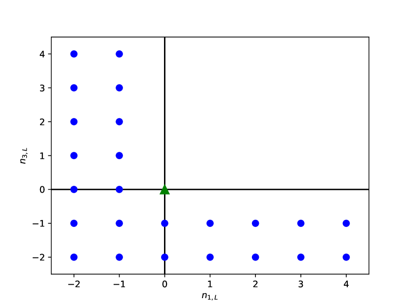
Figure 4: Prepare the arbitrarily normalized initial value (green triangle) and unitary condition (blue circle).

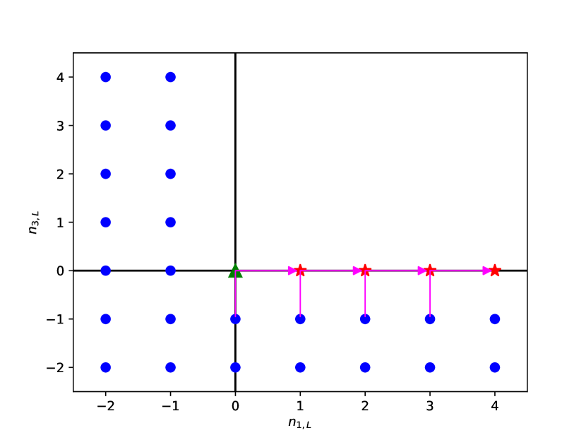
Figure 5: The recursion relation (A.157) with $n_{1,R}=n_{3,R}=0$ and $n_{3,L}=-1$ gives three-point function at horizontal axis.

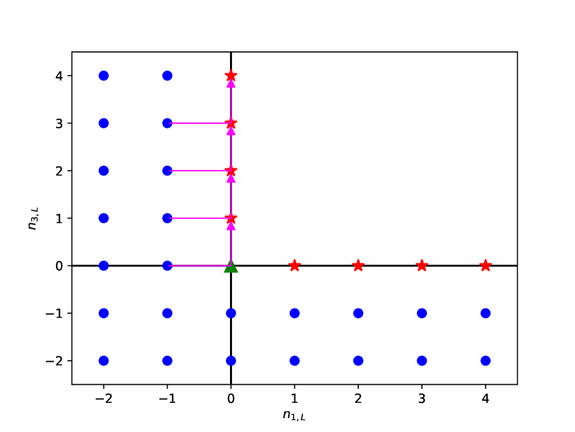
Figure 6: The recursion relation (A.158) with $n_{1,R}=n_{3,R}=0$ and $n_{1,L}=-1$ gives three-point functions at vertical axis.

Figure 7: The recursion ralation (A.157) with $n_{1,R}=n_{3,R}=0$ and $n_{3,L}=0$ gives three-point functions at $n_{3,L}=1$

Figure 8: The recursion ralation (A.158) with $n_{1,R}=n_{3,R}=0$ and $n_{1,L}=0$ gives three-point functions at $n_{1,L}=1$

Figure 9: We can get three-point functions at all points.

The derivation from the recursion relations of all three-point functions is summarized in the images. The horizontal axis represents $n_{1,L}$ and the vertical axis represents $n_{3,L}$.

First, prepare the arbitrarily normalized initial value $\mathcal{Y}3[h_{3,2,1},\tilde{h}_{3,2,1}|0,0,0,0]$, which is green triangle in the Fig. 5. From the unitarity condition, three-point functions at blue points vanish. At blue points, $n_{1,L}<0$ or $n_{3_{L}}<0$ is satisfied.

Next, from the recursion relation (A.157) with $n_{1,R}=n_{3,R}=0$ and $n_{3,L}=-1$, we can get three-point functions at horizontal axis (Fig. 5). And in the same way, three-point functions at the vertical axis can be calculated from the recursion relation (A.158) with $n_{1,R}=n_{3,R}=0$ and $n_{1,L}=-1$ (Fig. 7).

Recursion relation (A.157) with $n_{1,R}=n_{3,R}=0$ and $n_{3,L}=0$ gives three-point functions at $n_{3,L}=1$ (Fig. 7). And three-point functions at $n_{1,L}=1$ can be gotten in the same way (Fig. 9).

Finally, we can get three-point functions for all integer pairs of $(n_{1,L},n_{3,L},n_{1,R},n_{3,R})$ (Fig. 9).

Next, consider an explicit solution for the three-point functions.

First, start from the pair of nonnegative integer conformal weight $(h_{1,2,3},\tilde{h}_{1,2,3})$. In these particular cases, the three-point function factorizes globally rather than just locally into a product of a holomorphic and antiholomorphic three-point function. Fourier transform of three-point functions also factorizes and can be calculated individually by contour integration. We performed the contour integration in the previous appendix, and the result is

$$\mathcal{Y}3[h_{3,2,1},\tilde{h}_{3,2,1}|n_{3,L},n_{1,L},n_{3,R},n_{1,R}]$$

$$=K\mathcal{Y}3^{(\mathrm{chiral})}[h_{3,2,1}|n_{3,L},n_{1,L}]\mathcal{Y}3^{(\mathrm{antichiral})}[\tilde{h}_{3,2,1}|n_{3,R},n_{1,R}],$$

where $K$ is an unfixed constant related to the OPE coefficient. The chiral part for $n_{1,L},n_{3,L}\geq 0$ is

$$\mathcal{Y}3^{(\mathrm{chiral})}[h_{3,2,1}|n_{3,L},n_{1,L}]=\frac{1}{\Gamma(b_{1})\Gamma(b_{2})\Gamma(b_{3})}$$

$$\sum_{q=0}^{\mathrm{Min}\{n_{1,L},n_{3,L}\}}\tfrac{\Gamma[b_{3}+q+\mathrm{Max}\{{0,n_{1,L}-n_{3,L}}\}]\Gamma[b_{2}-q+\mathrm{Min}\{{n_{1,L},n_{3,L}}\}]\Gamma[b_{1}+q+\mathrm{Max}\{{n_{3,L}-n_{1,L},0}\}]}{\Gamma[1+q+\mathrm{Max}\{{0,n_{1,L}-n_{3,L}}\}]\Gamma[1-q+\mathrm{Min}\{{n_{1,L},n_{3,L}}\}]\Gamma[1+q+\mathrm{Max}\{{n_{3,L}-n_{1,L},0}\}]},$$ (A.165)

and $0$ for otherwise. And the antichiral part for $n_{1,R},n_{3,R}\geq 0$ is

$$\mathcal{Y}3^{(\mathrm{antichiral})}[\tilde{h}_{3,2,1}|n_{3,R},n_{1,R}]=\frac{1}{\Gamma(\tilde{b}_{1})\Gamma(\tilde{b}_{2})\Gamma(\tilde{b}_{3})}$$

$$\sum_{q=0}^{\mathrm{Min}\{n_{1,R},n_{3,R}\}}\tfrac{\Gamma[\tilde{b}_{3}+q+\mathrm{Max}\{{0,n_{1,R}-n_{3,R}}\}]\Gamma[\tilde{b}_{2}-q+\mathrm{Min}\{{n_{1,R},n_{3,R}}\}]\Gamma[\tilde{b}_{1}+q+\mathrm{Max}\{{n_{3,R}-n_{1,R},0}\}]}{\Gamma[1+q+\mathrm{Max}\{{0,n_{1,R}-n_{3,R}}\}]\Gamma[1-q+\mathrm{Min}\{{n_{1,R},n_{3,R}}\}]\Gamma[1+q+\mathrm{Max}\{{n_{3,R}-n_{1,R},0}\}]},$$ (A.166)

and $0$ for otherwise.

The contour integral derivation of (A.165) and (A.166) are only valid for a pair of nonnegative integers $(h_{3,2,1},\tilde{h}_{3,2,1})$.

We proved that any solution to the $L_{\pm 1}$ and $\tilde{L}_{\pm}$ WIs, which also satisfies the unitarity-derived condition, is uniquely determined by the primary-to-primary three-point coefficient $\mathcal{Y}3[h_{3,2,1},\tilde{h}_{3,2,1}|0,0,0,0]$. So what we have to do is only to prove that the formula (A.165) and (A.166) actually satisfy the WIs for general conformal weights.

In the previous section, we proved that the formula satisfies WIs. We dealt with positive integer conformal weights there, but we can use the same proof to show that WIs are satisfied for general conformal weights because we didn’t use the fact that conformal weights are positive integers there.

So the proof is completed. We can use our formula of the three-point function for operators with general conformal weights, except for negative integers.

Appendix B Supplement to three-dimensional CFT

B.1 Wigner $3j$ symbol

The Wigner $3j$ symbol is a more symmetric form of Clebsch-Gordan coefficients.

$$\matrixquantity(l_{1}&l_{2}&l_{3}\\ m_{1}&m_{2}&m_{3})\equiv\frac{(-1)^{l_{1}}}{\sqrt{2l_{3}+1}}\bra{l_{1},m_{1},l_{2},m_{2}}\ket{l_{3},-m_{3}}$$ (B.1)

It has the following properties. (1) Symmetry It is symmetric under an even permutation, but the phase factor appears under an odd permutation. For example, The $3j$ symbol is 0 unless all of the following conditions are met.

$$\text{(A)}\ \ m_{1}+m_{2}+m_{3}=0$$ (B.2)

$$\text{(B)}\ \ l_{1}+l_{2}+l_{3}\text{\ \ is an integer.}$$

$$\ \ \ \ \ \ \text{Moreover, an even integer if }m_{1}=m_{2}=m_{3}=0$$ (B.3)

$$\text{(C)}\ \ |m_{i}|\leq l_{i}$$ (B.4)

$$\text{(D)}\ \ |l_{1}-l_{2}|\leq l_{3}\leq|l_{1}+l_{2}|$$ (B.5)

(3) Relationship with spherical harmonics The $3j$ symbol is deeply related to the product of spherical harmonics.

The $3j$ symbols can be computed using the Racah formula.

$$\matrixquantity(l_{1}&l_{2}&l_{3}\\ m_{1}&m_{2}&m_{3})=(-1)^{l_{1}-l_{2}-l_{3}}\sqrt{\frac{(l_{1}+l_{2}-l_{3})!(l_{1}-l_{2}+l_{3})!(-l_{1}+l_{2}+l_{3})!}{(l_{1}+l_{2}+l_{3}+1)!}}$$

$$\sqrt{(l_{1}+m_{1})!(l_{1}-m_{1})!(l_{2}+m_{2})!(l_{2}-m_{2})!(l_{3}+m_{3})!(l_{3}-m_{3})!}$$

$$\sum_{k}\frac{(-1)^{k}}{k!(l_{3}-l_{2}+k+m_{1})!(l_{3}-l_{1}+k-m_{2})!(l_{1}+l_{2}-l_{3}-k)!(l_{1}-k-m_{1})!(l_{2}-k+m_{2})!}$$ (B.6)

Though the formula above is a little complicated, we often use the following specific simple case in this paper.

$$\matrixquantity(l_{1}&l_{2}&l_{1}+l_{2}\\ m_{1}&m_{2}&-m_{1}-m_{2})$$

$$=(-1)^{l_{1}-l_{2}+m_{1}+m_{2}}\sqrt{\frac{(2l_{1})!(2l_{2})!}{(2l_{1}+2l_{2}+1)!}}\sqrt{\frac{(l_{1}+l_{2}+m_{1}+m_{2})!(l_{1}+l_{2}-m_{1}-m_{2})!}{(l_{1}+m_{1})!(l_{1}-m_{1})!(l_{2}+m_{2})!(l_{2}-m_{2})!}}$$ (B.7)

Using them, we can calculate conformal generators’ action on spatially-integrated operators’ modes in three-dimensional CFT. Here, we show the calculation for $P_{x}+iP_{y}$ as an example. We can get relations for other generators similarly.

$$(P_{x}+iP_{y})\cdot\mathcal{O}_{l,m}=\int\differential\Omega Y^{*}_{l,m}(\theta,\phi)\left[\sin\theta e^{i\phi}\partialderivative{r}+\frac{\cos\theta}{r}e^{i\phi}\partialderivative{\theta}+i\frac{e^{i\phi}}{r\sin\theta}\partialderivative{\phi}\right]\mathcal{O}(r,\theta,\phi)$$ (B.8)

We calculate each term in (B.8) separately.

$$(\text{First term})=\int\differential\Omega Y^{*}_{l,m}(\theta,\phi)\sin\theta e^{i\phi}\partialderivative{r}\mathcal{O}(r,\theta,\phi)=-2\sqrt{\frac{2\pi}{3}}\partialderivative{r}\int\differential\Omega Y^{*}_{l,m}Y_{1,1}\mathcal{O}$$ (B.9)

$$(\text{Second term})=\int\differential\Omega Y^{*}_{l,m}(\theta,\phi)\frac{\cos\theta}{r}e^{i\phi}\partialderivative{\theta}\mathcal{O}(r,\theta,\phi)$$

$$=\frac{1}{r}\int\differential\theta\differential\phi\left[-\cos^{2}\theta Y^{*}_{l,m}+\sin^{2}\theta Y^{*}_{l,m}-\sin\theta\cos\theta\partialderivative{\theta}Y^{*}_{l,m}\right]e^{i\phi}\mathcal{O}$$

$$=\frac{1}{r}\int\differential\theta\differential\phi\left[-1+2\sin^{2}\theta-\cos\theta\{-m\cos\theta-\sin\theta\sqrt{(l+m)(l-m+1)}e^{-i\phi}\}\right]Y^{*}_{l,m}e^{i\phi}\mathcal{O}$$

$$=\frac{m-1}{r}\int\differential\theta\differential\phi Y^{*}_{l,m}e^{i\phi}\mathcal{O}+\frac{2(m-2)}{r}\sqrt{\frac{2\pi}{3}}\int\differential\Omega Y^{*}_{l,m}Y_{1,1}\mathcal{O}$$

$$\hskip 142.26378pt+\frac{2\sqrt{(l+m)(l-m+1)}}{r}\sqrt{\frac{\pi}{3}}\int\differential\Omega Y^{*}_{l,m-1}Y_{1,0}\mathcal{O}$$ (B.10)

$$(\text{Third term})=\int\differential\Omega Y^{*}_{l,m}(\theta,\phi)\frac{i}{r\sin\theta}e^{i\phi}\partialderivative{\phi}\mathcal{O}=-\frac{m-1}{r}\int\differential\theta\differential\phi Y^{*}_{l,m}e^{i\phi}\mathcal{O}$$ (B.11)

In total,

$$(P_{x}+iP_{y})\cdot\mathcal{O}_{l,m}$$

$$=2\sqrt{\frac{2\pi}{3}}\left(\frac{m-2}{r}-\partialderivative{r}\right)\int\differential\Omega Y^{*}_{l,m}Y_{1,1}\mathcal{O}+2\sqrt{\frac{\pi}{3}}\frac{\sqrt{(l+m)(l-m+1)}}{r}\int\differential\Omega Y^{*}_{l,m-1}Y_{1,0}\mathcal{O}$$ (B.12)

We would like to write the action of $P_{x}+iP_{y}$ by a linear combination of modes of operators, so let us apply the contraction rule to the product of spherical harmonics.

From (B.3) and (B.5), only $c=l\pm 1$ survive when $l\geq 1$, and only $c=1$ survives when $l=0$. And from (B.2), only $\gamma=-m$ survives.

$$Y^{*}_{l,m}Y_{1,0}=\sqrt{\frac{3(2l+1)}{4\pi}}\left[\sqrt{2l+3}\matrixquantity(l&1&l+1\\ -m&0&m)\matrixquantity(l&1&l+1\\ 0&0&0)Y_{l+1,-m}\right.\\ \left.+\sqrt{2l-1}\matrixquantity(l&1&l-1\\ -m&0&m)\matrixquantity(l&1&l-1\\ 0&0&0)Y_{l-1,-m}\right]$$ (B.13)

In the same way,

$$Y^{*}_{l,m}Y_{1,1}=-\sqrt{\frac{3(2l+1)}{4\pi}}\left[\sqrt{2l+3}\matrixquantity(l&1&l+1\\ -m&1&m-1)\matrixquantity(l&1&l+1\\ 0&0&0)Y_{l+1,-m+1}\right.\\ \left.+\sqrt{2l-1}\matrixquantity(l&1&l-1\\ -m&1&m-1)\matrixquantity(l&1&l-1\\ 0&0&0)Y_{l-1,-m+1}\right].$$ (B.14)

By using the above contraction rule, we get the following relation.

We can get the actions of other conformal generators similarly.

B.2 Exact two-point function

We show the detail of the calculation of exact two-point function in three-dimensional CFT by solving ODEs obtained from WIs. First, consider the $P_{z}$ WI.

The first and fourth terms have $\delta(l_{1}-l_{2}-1)$, and the second and third have $\delta(l_{1}-l_{2}+1)$. We have two independent recursion relations for them. From the latter, we get

$$0=y\left[\matrixquantity(l_{1}&1&l_{1}+1\\ 0&0&0)\left(-y\derivative{y}-\Delta_{2}+2\right)+\sqrt{2}\matrixquantity(l_{1}&1&l_{1}+1\\ 0&-1&1)\sqrt{(l_{1}+1)(l_{1}+2)}\right]G^{l_{1}}\\ +\left[\matrixquantity(l_{1}&1&l_{1}+1\\ 0&0&0)\left(y\derivative{y}-\Delta_{1}+2\right)+\sqrt{2}\matrixquantity(l_{1}&1&l_{1}+1\\ 1&-1&0)\sqrt{l_{1}(l_{1}+1)}\right]G^{l_{1}+1}.$$ (B.15)

And from the $K_{z}$ WI, we get

$$0=y\left[\matrixquantity(l_{1}&1&l_{1}+1\\ 0&0&0)\left(y\derivative{y}+\Delta_{1}-2\right)-\sqrt{2}\matrixquantity(l_{1}&1&l_{1}+1\\ 0&-1&1)\sqrt{(l_{1}+1)(l_{1}+2)}\right]G^{l_{1}}\\ +\left[\matrixquantity(l_{1}&1&l_{1}+1\\ 0&0&0)\left(-y\derivative{y}+\Delta_{2}-2\right)-\sqrt{2}\matrixquantity(l_{1}&1&l_{1}+1\\ 1&-1&0)\sqrt{l_{1}(l_{1}+1)}\right]G^{l_{1}+1}.$$ (B.16)

From (B.15) and (B.16), we get

$$(\Delta_{1}-\Delta_{2})[yG^{l_{1}}-G^{l_{1}+1}]=0.$$ (B.17)

First, assume that $G^{l_{1}+1}=yG^{l_{1}}$ is satisfied. Substituting it for (B.15) yields

$$(\Delta_{1}+\Delta_{2}+1)yG^{l_{1}}=0.$$ (B.18)

However, as $\Delta_{1}+\Delta_{2}+1>0$, $G^{l_{1}}$ must vanish. So $\Delta_{1}=\Delta_{2}$ must be satisfied for two-point function not to vanish. Next, consider $P_{x}\pm iP_{y}$ and $K_{x}+iK_{y}$ WIs. There are only two independent identities.

$$0=\left[\sqrt{2}\matrixquantity(l&1&l+1\\ -1&1&0)\left(y\derivative{y}-\Delta+2\right)+\matrixquantity(l&1&l+1\\ -1&0&1)\sqrt{(l+2)(l+1)}\right]G^{l}\\ +y\left[\sqrt{2}\matrixquantity(l&1&l+1\\ -1&1&0)\left(-y\derivative{y}-\Delta+1\right)+\matrixquantity(l&1&l+1\\ 0&0&0)\sqrt{(l+1)l}\right]G^{l+1}$$ (B.21)

$$0=y\left[\sqrt{2}\matrixquantity(l&1&l+1\\ -1&1&0)\left(y\derivative{y}+\Delta-2\right)-\matrixquantity(l&1&l+1\\ -1&0&1)\sqrt{(l+2)(l+1)}\right]G^{l}\\ +\left[\sqrt{2}\matrixquantity(l&1&l+1\\ -1&1&0)\left(-y\derivative{y}+\Delta-1\right)-\matrixquantity(l&1&l+1\\ 0&0&0)\sqrt{(l+1)l}\right]G^{l+1}$$ (B.23)

Substituting the explicit form of the Wigner $3j$ symbol, we get

$$\left[y\derivative{y}-\Delta+l+2\right]G^{l+1}+y\left[-y\derivative{y}-\Delta-l\right]G^{l}=0$$ (B.24)

$$y\left[-y\derivative{y}-\Delta+l+2\right]G^{l+1}+\left[y\derivative{y}-\Delta-l\right]G^{l}=0.$$ (B.25)

Combining them gives

$$\derivative[2]{y}G^{l}+\frac{2\Delta y^{2}+2(\Delta-1)}{y^{3}-y}\derivative{y}G^{l}+\frac{\Delta(\Delta-1)}{y^{2}}G^{l}=0.$$ (B.26)

It is very similar to the ODE (A.16) for the two-point function in two-dimensional CFT. We can solve it by series expansion as we did in two-dimensional CFT. The answer is shown in the main text.

B.3 Reduction of the three-point function

B.3.1 Strategy

In the calculation of the two-point functions in three-dimensional CFT, we found that the ODE (LABEL:ODE_for_two_pt_func_in_3_dim) obtained from the WIs was independent of the subscripts $m_{1}$ and $m_{2}$ because of the linear relationship (LABEL:Jpm_Ward_Identity_result) between $F_{m1}^{l_{1},l_{2}}$ and $F_{m_{1}+1}^{l_{1},l_{2}}$. Similarly, we can get a linear relationship between $F_{m_{1},m_{3}}^{l_{1},l_{2},l_{3}}$ and $F_{m^{\prime}_{1},m^{\prime}_{3}}^{l_{1},l_{2},l_{3}}$, which enables us to get the simpler ODEs.

First, remember that the $J_{x}+iJ_{y}$ WI relates $F_{m_{1},m_{3}}^{l_{1},l_{2},l_{3}}$, $F_{m_{1}-1,m_{3}}^{l_{1},l_{2},l_{3}}$ and $F_{m_{1},m_{3}-1}^{l_{1},l_{2},l_{3}}$, and that the $J_{x}-iJ_{y}$ WI relates $F_{m_{1},m_{3}}^{l_{1},l_{2},l_{3}}$, $F_{m_{1}+1,m_{3}}^{l_{1},l_{2},l_{3}}$ and $F_{m_{1},m_{3}+1}^{l_{1},l_{2},l_{3}}$. The situation can be explained graphically. The Fig. 10 shows examples of how $J_{x}\pm iJ_{y}$ relates $F_{m_{1},m_{3}}^{l_{1},l_{2},l_{3}}$ at three points in the $m_{1}-m_{3}$ plane. In the figure, for example, if we know the value of $F_{1,0}^{l_{1},l_{2},l_{3}}$ and $F_{1,1}^{l_{1},l_{2},l_{3}}$, we can derive $F_{1,0}^{l_{1},l_{2},l_{3}}$ with the $J_{x}+iJ_{y}$ WI.

Figure 10: $J_{x}+iJ_{y}$ relates three points connected by the blue line, and $J_{x}-iJ_{y}$ relates three points connected by the red line.

Next, consider the selection rule for $F_{m_{1},m_{3}}^{l_{1},l_{2},l_{3}}$. Prepare $l_{1}$, $l_{2}$ and $l_{3}$ which satisfy $|l_{1}-l_{2}|\leq l_{3}\leq l_{1}+l_{2}$ , $|l_{2}-l_{3}|\leq l_{1}\leq l_{2}+l_{3}$ and $|l_{3}-l_{1}|\leq l_{2}\leq l_{3}+l_{1}$. For this fixed pairs of $l$, the rule is as follows. $F_{m_{1},m_{3}}^{l_{1},l_{2},l_{3}}$ vanishes unless the all following inequalities are satisfied.

$$-l_{1}\leq m_{1}\leq l_{1},\hskip 28.45274pt-l_{3}\leq m_{3}\leq l_{3},\hskip 28.45274pt-l_{2}\leq m_{1}+m_{3}\leq l_{2}$$ (B.27)

The last condition comes from $m_{2}=-m_{1}-m_{3}$ and $-l_{2}\leq m_{2}\leq l_{2}$. The area which satisfies the above conditions is diamond-shaped as Fig. 11.

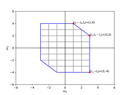
Figure 11: Example of selection rule $(l_{1},l_{2},l_{3})=(3,4,5)$. $F_{m_{1},m_{3}}^{l_{1},l_{2},l_{3}}$ vanish in areas outside the blue line.

Our goal is to get all $F_{m_{1},m_{3}}^{l_{1},l_{2},l_{3}}$s in this area using $F_{l_{1},-l_{3}}^{l_{1},l_{2},l_{3}}$ and the recursion relations obtained from $J\pm iJ_{y}$ WIs.

First, apply the $J_{x}-iJ_{y}$ recursion relation to $(m_{1},m_{3})=(l_{1},-l_{3}+k)\ (0\leq k\leq l_{2}-l_{1}-l_{3}-1)$. $F_{m_{1}+1,m_{3}}^{l_{1},l_{2},l_{3}}$ vanishes for this $m_{1}$ and $m_{3}$, so the $J_{x}-iJ_{y}$ recursion relation relates two points. We can find all the values of $F$ at the right boundary. Similarly, we can find all the values of $F$ at the bottom boundary. We show the situation in the Fig. 12.

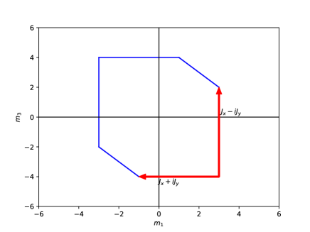
Figure 12: We can get the $F$s at the right boundary and at the bottom boundary by applying $J_{x}\pm iJ_{y}$ WIs respectively.

Next, apply the $J_{x}-iJ_{y}$ WI to the right part of the area and apply the $J_{x}+iJ_{y}$ WI to the left part of the area Fig. 14 and Fig. 14. Then we can find all the $F$s in the area.

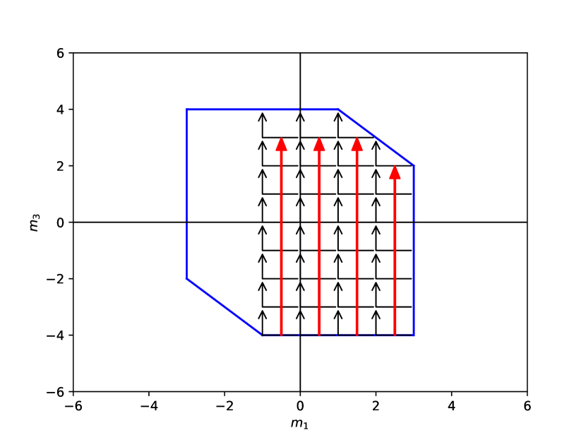
Figure 13: Apply the $J_{x}-iJ_{y}$ WI to the right part of the area

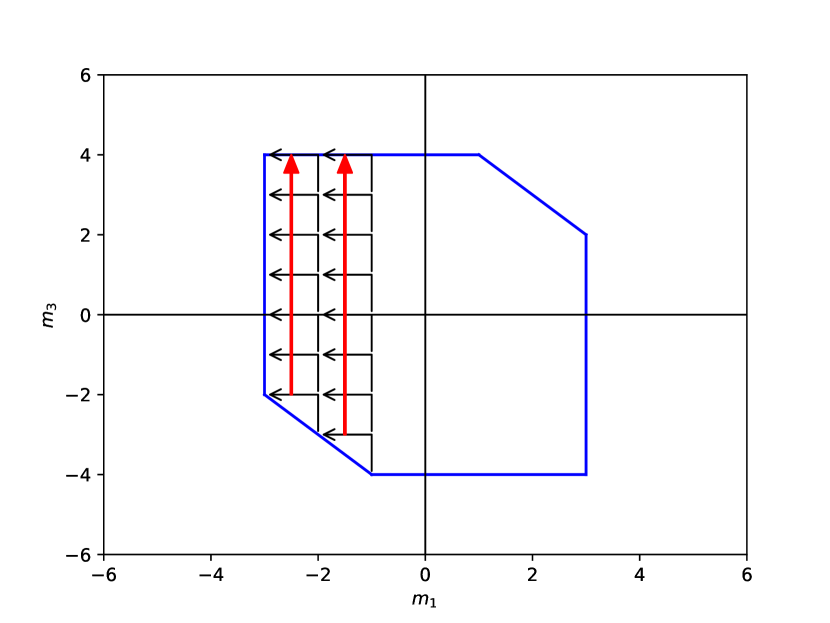
Figure 14: Apply the $J_{x}+iJ_{y}$ WI to the left part of the area

B.3.2 Solution

Now that we know the strategy, all we have to do is solve the recursion relations. Applying the $J_{x}-iJ_{y}$ WI to the right boundary gives

$$F_{l_{1},-l_{3}+k}^{l_{1},l_{2},l_{3}}=(-1)^{k}\sqrt{\frac{(l_{2}-l_{1}+l_{3})!(l_{2}+l_{1}-l_{3}+k)!(2l_{3}-k)!}{(l_{2}-l_{1}+l_{3}-k)!(l_{2}+l_{1}-l_{3})!(2l_{3})!k!}}F_{l_{1},-l_{3}}^{l_{1},l_{2},l_{3}}.$$ (B.28)

And applying the $J_{x}+iJ_{y}$ WI to the bottom boundary gives

$$F_{l_{1}-n,-l_{3}}^{l_{1},l_{2},l_{3}}=(-1)^{n}\sqrt{\frac{(l_{2}+l_{1}-l_{3})!(l_{2}-l_{1}+l_{3}+n)!(2l_{1}-n)!}{(l_{2}+l_{1}-l_{3}-n)!(l_{2}-l_{1}+l_{3})!(2l_{1})!n!}}F_{l_{1},-l_{3}}^{l_{1},l_{2},l_{3}}.$$ (B.29)

Next, applying the $J_{x}+iJ_{y}$ WI to $m_{1}=l_{1},m_{3}=-l_{3}+k$ gives

$$F_{l_{1}-1,-l_{3}+k}=\frac{(-1)^{k}}{\sqrt{2l_{1}}}\sqrt{\frac{(l_{2}-l_{1}+l_{3})!(l_{2}+l_{1}-l_{3}+k-1)!(2l_{3}-k)!}{(l_{2}-l_{1}+l_{3}-k+1)!(l_{2}+l_{1}-l_{3})!(2l_{3})!k!}}\\ [2l_{1}k-(l_{2}+l_{1}-l_{3})(l_{2}-l_{1}+l_{3}+1)]F_{l_{1},-l_{3}}^{l_{1},l_{2},l_{3}}.$$ (B.32)

And applying the $J_{x}+iJ_{y}$ WI to $m_{1}=l_{1}-1,m_{3}=-l_{3}+k$ gives

$$F_{l_{1}-2,-l_{3}+k}=\frac{(-1)^{k+1}}{2\sqrt{l_{1}(2l_{1}-1)}}\sqrt{\frac{(l_{2}-l_{1}+l_{3})!(l_{2}+l_{1}-l_{3}+k-2)!(2l_{3}-k)!}{(l_{2}-l_{1}+l_{3}-k+2)!(l_{2}+l_{1}-l_{3})!(2l_{3})!k!}}[2l_{1}k(2l_{3}-k+1)-$$

$$\{2l_{1}k-(l_{2}+l_{1}-l_{3})(l_{2}-l_{1}+l_{3}+1)\}\{2(l_{1}-1)k-(l_{2}+l_{1}-l_{3}-1)(l_{2}-l_{1}+l_{3}+2)\}]F_{l_{1},-l_{3}}^{l_{1},l_{2},l_{3}}.$$ (B.33)

They induce us to write $F_{l_{1}-n,-l_{3}+k}^{l_{1},l_{2},l_{3}}$ as

$$F_{l_{1}-n,-l_{3}+k}^{l_{1},l_{2},l_{3}}=(-1)^{k}\sqrt{\frac{(2l_{1}-n)!(2l_{3}-k)!(l_{2}-l_{1}+l_{3})!(l_{2}+l_{1}-l_{3}+k-n)!}{(2l_{1})!n!(2l_{3})!k!(l_{2}-l_{1}+l_{3}-k+n)!(l_{2}+l_{1}-l_{3})!}}f_{n,k}F_{l_{1},-l_{3}}^{l_{1},l_{2},l_{3}}.$$ (B.34)

The $J_{x}\pm iJ_{y}$ recursion relations for this $f_{n,k}$ are

$$f_{n+1,k} =k(2l_{3}-k+1)f_{n,k-1}-(l_{2}+l_{1}-l_{3}-n+k)(l_{2}-l_{1}+l_{3}+n-k+1)f_{n,k}$$ (B.35)

$$f_{n,k+1} =n(2l_{1}-n+1)f_{n-1,k}+f(n,k).$$ (B.36)

From its definition, $f_{0,k}=1$. The following results can be obtained from actual calculations using the recursion relations.

$$f_{n,0} =(-1)^{n}\frac{(l_{2}+l_{1}-l_{3})!(l_{2}-l_{1}+l_{3}+n)!}{(l_{2}+l_{1}-l_{3}-n)!(l_{2}-l_{1}+l_{3})!}$$ (B.37)

$$f_{n,1} =(-1)^{n}\frac{(l_{2}+l_{1}-l_{3}+1)!(l_{2}-l_{1}+l_{3}+n-1)!}{(l_{2}+l_{1}-l_{3}-n+1)!(l_{2}-l_{1}+l_{3}-1)!}$$

$$\hskip 14.22636pt+(-1)^{n-1}\frac{(l_{2}+l_{1}-l_{3})!(l_{2}-l_{1}+l_{3}+n-1)!}{(l_{2}+l_{1}-l_{3}-n+1)!(l_{2}-l_{1}+l_{3})!}2nl_{3}$$ (B.38)

$$f_{n,2} =(-1)^{n}\frac{(l_{2}+l_{1}-l_{3}+2)!(l_{2}-l_{1}+l_{3}+n-2)!}{(l_{2}+l_{1}-l_{3}-n+2)!(l_{2}-l_{1}+l_{3}-2)!}$$

$$\hskip 14.22636pt+(-1)^{n-1}\frac{(l_{2}+l_{1}-l_{3}+1)!(l_{2}-l_{1}+l_{3}+n-2)!}{(l_{2}+l_{1}-l_{3}-n+2)!(l_{2}-l_{1}+l_{3}-1)!}2n(2l_{3}-1)$$

$$\hskip 14.22636pt+(-1)^{n}\frac{(l_{2}+l_{1}-l_{3})!(l_{2}-l_{1}+l_{3}+n-2)!}{(l_{2}+l_{1}-l_{3}-n+2)!(l_{2}-l_{1}+l_{3})!}n(n-1)2l_{3}(2l_{3}-1)$$ (B.39)

$$f_{n,3} =(-1)^{n}\frac{(l_{2}+l_{1}-l_{3}+3)!(l_{2}-l_{1}+l_{3}+n-3)!}{(l_{2}+l_{1}-l_{3}-n+3)!(l_{2}-l_{1}+l_{3}-3)!}$$

$$\hskip 14.22636pt+(-1)^{n-1}\frac{(l_{2}+l_{1}-l_{3}+2)!(l_{2}-l_{1}+l_{3}+n-3)!}{(l_{2}+l_{1}-l_{3}-n+3)!(l_{2}-l_{1}+l_{3}-2)!}3n(2l_{3}-2)$$

$$\hskip 14.22636pt+(-1)^{n}\frac{(l_{2}+l_{1}-l_{3}+1)!(l_{2}-l_{1}+l_{3}+n-3)!}{(l_{2}+l_{1}-l_{3}-n+3)!(l_{2}-l_{1}+l_{3}-1)!}3n(n-1)(2l_{3}-1)(2l_{3}-2)$$

$$\hskip 14.22636pt+(-1)^{n-1}\frac{(l_{2}+l_{1}-l_{3})!(l_{2}-l_{1}+l_{3}+n-3)!}{(l_{2}+l_{1}-l_{3}-n+3)!(l_{2}-l_{1}+l_{3})!}n(n-1)(n-2)2l_{3}(2l_{3}-1)(2l_{3}-2)$$

From them, we can assume that $f_{n,k}$ has the following form.

$$f_{n,k} =\sum_{l=0}^{k}P_{n,k,l}(-1)^{n-l}\frac{(l_{2}+l_{1}-l_{3}+k-l)!(l_{2}-l_{1}+l_{3}+n-k)!}{(l_{2}+l_{1}-l_{3}-n+k)!(l_{2}-l_{1}+l_{3}-k+l)!}$$ (B.41)

$$P_{n,k,l} ={}_{k}C_{l}\frac{n!}{(n-l)!}\frac{(2l_{3}-k+l)!}{(2l_{3}-k)!}=\frac{k!n!(2l_{3}-k+l)!}{l!(k-l)!(n-l)!(2l_{3}-k)!}$$ (B.42)

We prove it by mathematical induction. First, the above configuration is consistent with the result for $(n,k)=(n,0)$ shown in (B.29). The recursion relations of $P_{n,k,l}$ for $k$ are

$$P_{n,k+1,0}=P_{n,k,0}=1$$ (B.43)

$$P_{n,k+1,1}=P_{n,k,1}-n(2l_{1}-2l_{3}-n+2k+1)P_{n,k,0}+n(2l_{1}-n+1)P_{n-1,k,0}$$ (B.44)

$$P_{n,k+1,2}=P_{n,k,2}-(n-1)(2l_{1}-2l_{3}-n+2k)P_{n,k,1}+n(2l_{1}-n+1)P_{n-1,k,1}$$ (B.45)

$$\cdots$$

$$P_{n,k+1,k}=P_{n,k,k}-(n-k)(2l_{1}-2l_{3}-n+k+2)P_{n,k,0}+n(2l_{1}-n+1)P_{n-1,k,k-1}$$ (B.46)

$$P_{n,k+1,k+1}=-(n-k)(2l_{1}-2l_{3}-n+k+1)P_{n,k,k}+n(2l_{1}-n+1)P_{n-1,k,k}.$$ (B.47)

Assume that the above configuration (B.41) and (B.42) are correct for $k\geq 0$. Then, from the above recursion relations, we get

$$P_{n,k+1,0}=1$$ (B.48)

$$P_{n,k+1,m}=P_{n,k,m}-(n-m+1)(2l_{1}-2l_{3}-n+2k+2-m)P_{n,k,m-1}+n(2l_{1}-n+1)P_{n-1,k,m-1}$$

$$={}_{k}C_{m}\frac{n!}{(n-m)!}\frac{(2l_{3}-k+m)!}{(2l_{3}-k)!}+n{}_{k}C_{m-1}\frac{(n-1)!}{(n-m)!}\frac{(2l_{3}-k+m-1)!}{(2l_{3}-k)!}(2l_{1}-n+1)$$

$$\hskip 14.22636pt-(n-m+1){}_{k}C_{m-1}\frac{n!}{(n-m+1)!}\frac{(2l_{3}-k+m-1)!}{(2l_{3}-k)!}(2l_{1}-2l_{3}-n+2k+2-m)$$

$$={}_{k+1}C_{m}\frac{n!}{(n-m)!}\frac{(2l_{3}-k-1+m)!}{(2l_{3}-k-1)!}\hskip 28.45274pt(1\leq m\leq k)$$ (B.49)

$$P_{n,k+1,k+1}$$

$$=-(n-k)(2l_{1}-2l_{3}-n+k+1)\frac{n!}{(n-k)!}\frac{(2l_{3})!}{(2l_{3}-k)!}+n(2l_{1}-n+1)\frac{(n-1)!}{(n-k-1)!}\frac{(2l_{3})!}{(2l_{3}-k)!}$$

$$=\frac{n!}{(n-k-1)!}\frac{(2l_{3})!}{(2l_{3}-k-1)!}.$$ (B.50)

So, the configuration (B.41) and (B.42) are also correct for $k+1$.

The conclusion is

$$F_{l_{1}-n,-l_{3}+k}^{l_{1},l_{2},l_{3}} =(-1)^{n+k}\sqrt{\frac{(2l_{1}-n)!(2l_{3}-k)!(l_{2}-l_{1}+l_{3})!(l_{2}+l_{1}-l_{3}+k-n)!}{(2l_{1})!n!(2l_{3})!k!(l_{2}-l_{1}+l_{3}-k+n)!(l_{2}+l_{1}-l_{3})!}}f_{n,k}F_{l_{1},-l_{3}}^{l_{1},l_{2},l_{3}}$$ (B.51)

$$f_{n,k} =\sum_{l=0}^{k}P_{n,k,l}(-1)^{l}\frac{(l_{2}+l_{1}-l_{3}+k-l)!(l_{2}-l_{1}+l_{3}+n-k)!}{(l_{2}+l_{1}-l_{3}-n+k)!(l_{2}-l_{1}+l_{3}-k+l)!}$$ (B.52)

$$P_{n,k,l} =\frac{k!n!(2l_{3}-k+l)!}{l!(k-l)!(n-l)!(2l_{3}-k)!}.$$ (B.53)

B.4 Direct integral calculation of three-point function

In two-dimensional CFT, the direct integral calculation is straightforward because we can decompose it into holomorphic and antiholomorphic parts. We can calculate them independently by a complex integral technique. On the other hand, in three-dimensional CFT, we don’t have such techniques, so we have to perform direct integral calculations straightforwardly. From the definition,

$$\int\frac{\differential\Omega_{1}}{4\pi}\int\frac{\differential\Omega_{2}}{4\pi}\int\frac{\differential\Omega_{3}}{4\pi} \langle\mathcal{O}_{3}\mathcal{O}_{2}\mathcal{O}_{1}\rangle=\lambda_{321}r_{1}^{-\Delta_{1}}r_{2}^{-\Delta_{2}}r_{3}^{-\Delta_{3}}\sum_{p,q\in\mathbb{Z}_{\geq 0}}F_{(p,q)}^{000}y_{1}^{\Delta_{1}+2p}y_{3}^{-\Delta_{3}-2q}$$

$$=\int\frac{\differential\Omega_{1}}{4\pi}\int\frac{\differential\Omega_{2}}{4\pi}\int\frac{\differential\Omega_{3}}{4\pi}\frac{\lambda_{321}}{x_{12}^{\Delta_{1}+\Delta_{2}-\Delta_{3}}x_{23}^{\Delta_{2}+\Delta_{3}-\Delta_{1}}x_{31}^{\Delta_{3}+\Delta_{1}-\Delta_{2}}},$$ (B.54)

where $x_{ij}^{2}=r_{i}^{2}+r_{j}^{2}-2r_{i}r_{j}\Phi_{ij}$. We can obtain $F_{(p,q)}^{000}$ by differentiating it.

$$F_{(p,q)}^{000}= \int\frac{\differential\Omega_{1}}{4\pi}\int\frac{\differential\Omega_{2}}{4\pi}\int\frac{\differential\Omega_{3}}{4\pi}\frac{1}{(2p)!}\frac{1}{(2q)!}\left(\derivative{z_{1}}\right)^{2p}\left(\derivative{z_{3}}\right)^{2q}$$

$$(1+z_{1}^{2}-2z_{1}\Phi_{12})^{g_{12}}(1+z_{3}^{2}-2z_{3}\Phi_{23})^{g_{23}}(1+(z_{1}z_{3})^{2}-2z_{1}z_{3}\Phi_{31})^{g_{31}}|_{z_{1}=z_{3}=0}$$ (B.55)

To calculate it, we need the following relation.

$$\left.\frac{1}{(2q)!}\left(\derivative{z}\right)^{2q}(1+z^{2}-2z\Phi)^{g}\right|_{z=0}=\sum_{k=0}^{q}\frac{2^{2k}}{(q-k)!(2k)!}\frac{g!}{(g-q-k)!}\Phi^{2k}$$ (B.56)

We omit its derivation here. With this, calculate the amplitude $F_{(p,q)}^{000}$. First, consider the differentiation by $z_{3}$.

$$\left(\derivative{z_{3}}\right)^{2q}(1+z_{3}^{2}-2z_{3}\Phi_{23})^{g_{23}}(1+(z_{1}z_{3})^{2}-2z_{1}z_{3}\Phi_{31})^{g_{31}}$$

$$= \sum_{k=0}^{q}\sum_{j=0}^{k}\sum_{l=0}^{q-k}\frac{2^{2(j+l)}(2q)!}{(k-j)!(2j)!(q-k-l)!(2l)!}\frac{g_{31}!g_{23}!\Phi_{31}^{2j}\Phi_{23}^{2l}}{(g_{31}-k-j)!(g_{23}-q+k-l)!}z_{1}^{2k}$$

$$+ \sum_{k=0}^{q-1}\sum_{j=0}^{k}\sum_{l=0}^{q-k-1}\frac{2^{2(j+l+1)}(2q)!}{(k-j)!(2j+1)!(q-k-l-1)!(2l+1)!}\frac{g_{31}!g_{23}!\Phi_{31}^{2j+1}\Phi_{23}^{2l+1}}{(g_{31}-k-j-1)!(g_{23}-q+k-l)!}z_{1}^{2k+1}$$ (B.57)

Next, consider the differentiation by $z_{1}$.

$$\left.\left(\derivative{z_{1}}\right)^{2p}(1+z_{1}^{2}-2z_{1}\Phi_{12})^{g_{12}}z_{1}^{2k}\right|_{z_{1}=0}\begin{cases}0&(p<k)\\ \sum_{n=0}^{p-k}\frac{2^{2n}(2p)!}{(p-k-n)!(2n)!}\frac{g_{12}!\Phi_{12}^{2n}}{(g_{12}-p+k-n)!}&(p\geq k)\end{cases}$$ (B.58)

$$\left.\left(\derivative{z_{1}}\right)^{2p}(1+z_{1}^{2}-2z_{1}\Phi_{12})^{g_{12}}z_{1}^{2k+1}\right|_{z_{1}=0}=\begin{cases}0&(p\leq k)\\ \sum_{n=0}^{p-k-1}\frac{-2^{2n+1}(2p)!}{(p-k-n-1)!(2n+1)!}\frac{g_{12}!\Phi_{12}^{2n+1}}{(g_{12}-p+k-n)!}&(p>k)\end{cases}$$ (B.59)

With them, we get

$$F_{(p,q)}^{000}= \sum_{k=0}^{\min(p,q)}\sum_{j=0}^{k}\sum_{n=0}^{p-k}\sum_{l=0}^{q-k}A_{k,j,n,l}\int\frac{\differential\Omega_{1}}{4\pi}\int\frac{\differential\Omega_{2}}{4\pi}\int\frac{\differential\Omega_{3}}{4\pi}\Phi_{12}^{2n}\Phi_{23}^{2l}\Phi_{31}^{2j}$$

$$-\sum_{k=0}^{\min(p-1,q-1)}\sum_{j=0}^{k}\sum_{n=0}^{p-k-1}\sum_{l=0}^{q-k-1}B_{k,j,n,l}\int\frac{\differential\Omega_{1}}{4\pi}\int\frac{\differential\Omega_{2}}{4\pi}\int\frac{\differential\Omega_{3}}{4\pi}\Phi_{12}^{2n+1}\Phi_{23}^{2l+1}\Phi_{31}^{2j+1},$$ (B.60)

where

$$A_{k,j,n,l}= \tfrac{2^{2(j+n+l)}}{(2j)!(2n)!(2l)!(k-j)!(p-k-n)!(q-k-l)!}\tfrac{g_{12}!g_{23}!g_{31}!}{(g_{31}-k-j)!(g_{12}-p+k-n)!(g_{23}-q+k-l)!}$$ (B.61)

$$B_{k,j,n,l}= \tfrac{2^{2(j+n+l)+3}}{(2j+1)!(2n+1)!(2l+1)!(k-j)!(p-k-n-1)!(q-k-l-1)!}\tfrac{g_{12}!g_{23}!g_{31}!}{(g_{31}-k-j-1)!(g_{12}-p+k-n)!(g_{23}-q+k-l)!}.$$ (B.62)

References

- [AABP17] Ofer Aharony, Luis F. Alday, Agnese Bissi, and Eric Perlmutter. Loops in AdS from Conformal Field Theory. JHEP, 07:036, 2017. arXiv:1612.03891, doi:10.1007/JHEP07(2017)036.
- [AB17] Luis F. Alday and Agnese Bissi. Loop Corrections to Supergravity on . Phys. Rev. Lett., 119(17):171601, 2017. arXiv:1706.02388, doi:10.1103/PhysRevLett.119.171601.
- [ACDR09] Roberta Armillis, Claudio Coriano, and Luigi Delle Rose. Anomaly Poles as Common Signatures of Chiral and Conformal Anomalies. Phys. Lett. B, 682:322–327, 2009. arXiv:0909.4522, doi:10.1016/j.physletb.2009.11.013.
- [ACDR10a] Roberta Armillis, Claudio Coriano, and Luigi Delle Rose. Conformal Anomalies and the Gravitational Effective Action: The TJJ Correlator for a Dirac Fermion. Phys. Rev. D, 81:085001, 2010. arXiv:0910.3381, doi:10.1103/PhysRevD.81.085001.
- [ACDR10b] Roberta Armillis, Claudio Coriano, and Luigi Delle Rose. Trace Anomaly, Massless Scalars and the Gravitational Coupling of QCD. Phys. Rev. D, 82:064023, 2010. arXiv:1005.4173, doi:10.1103/PhysRevD.82.064023.
- [ACH18] Luis F. Alday and Simon Caron-Huot. Gravitational S-matrix from CFT dispersion relations. JHEP, 12:017, 2018. arXiv:1711.02031, doi:10.1007/JHEP12(2018)017.
- [ADHP18] F. Aprile, J. M. Drummond, P. Heslop, and H. Paul. Quantum Gravity from Conformal Field Theory. JHEP, 01:035, 2018. arXiv:1706.02822, doi:10.1007/JHEP01(2018)035.
- [AHMNV07] Nima Arkani-Hamed, Lubos Motl, Alberto Nicolis, and Cumrun Vafa. The String landscape, black holes and gravity as the weakest force. JHEP, 06:060, 2007. arXiv:hep-th/0601001, doi:10.1088/1126-6708/2007/06/060.
- [AMM97] Ignatios Antoniadis, Pawel O. Mazur, and Emil Mottola. Conformal invariance and cosmic background radiation. Phys. Rev. Lett., 79:14–17, 1997. arXiv:astro-ph/9611208, doi:10.1103/PhysRevLett.79.14.
- [AMM12] Ignatios Antoniadis, Pawel O. Mazur, and Emil Mottola. Conformal Invariance, Dark Energy, and CMB Non-Gaussianity. JCAP, 09:024, 2012. arXiv:1103.4164, doi:10.1088/1475-7516/2012/09/024.
- [BDBM20] Mert Beşken, Jan De Boer, and Grégoire Mathys. On local and integrated stress-tensor commutators. JHEP, 21:148, 2020. arXiv:2012.15724, doi:10.1007/JHEP07(2021)148.
- [BG20] Teresa Bautista and Hadi Godazgar. Lorentzian CFT 3-point functions in momentum space. JHEP, 01:142, 2020. arXiv:1908.04733, doi:10.1007/JHEP01(2020)142.
- [BMS14] Adam Bzowski, Paul McFadden, and Kostas Skenderis. Implications of conformal invariance in momentum space. JHEP, 03:111, 2014. arXiv:1304.7760, doi:10.1007/JHEP03(2014)111.
- [BPZ84] A. A. Belavin, Alexander M. Polyakov, and A. B. Zamolodchikov. Infinite Conformal Symmetry in Two-Dimensional Quantum Field Theory. Nucl. Phys. B, 241:333–380, 1984. doi:10.1016/0550-3213(84)90052-X.
- [CDRMS13] Claudio Coriano, Luigi Delle Rose, Emil Mottola, and Mirko Serino. Solving the Conformal Constraints for Scalar Operators in Momentum Space and the Evaluation of Feynman’s Master Integrals. JHEP, 07:011, 2013. arXiv:1304.6944, doi:10.1007/JHEP07(2013)011.
- [CDRQS11] Claudio Coriano, Luigi Delle Rose, Antonio Quintavalle, and Mirko Serino. The Conformal Anomaly and the Neutral Currents Sector of the Standard Model. Phys. Lett. B, 700:29–38, 2011. arXiv:1101.1624, doi:10.1016/j.physletb.2011.04.053.
- [CDRS11] Claudio Coriano, Luigi Delle Rose, and Mirko Serino. Gravity and the Neutral Currents: Effective Interactions from the Trace Anomaly. Phys. Rev. D, 83:125028, 2011. arXiv:1102.4558, doi:10.1103/PhysRevD.83.125028.
- [Che19] Shai M. Chester. Weizmann Lectures on the Numerical Conformal Bootstrap. 7 2019. arXiv:1907.05147.
- [CHT19] Simon Caron-Huot and Anh-Khoi Trinh. All tree-level correlators in AdS5×S5 supergravity: hidden ten-dimensional conformal symmetry. JHEP, 01:196, 2019. arXiv:1809.09173, doi:10.1007/JHEP01(2019)196.
- [ESPP+12] Sheer El-Showk, Miguel F. Paulos, David Poland, Slava Rychkov, David Simmons-Duffin, and Alessandro Vichi. Solving the 3D Ising Model with the Conformal Bootstrap. Phys. Rev. D, 86:025022, 2012. arXiv:1203.6064, doi:10.1103/PhysRevD.86.025022.
- [ESPP+14] Sheer El-Showk, Miguel F. Paulos, David Poland, Slava Rychkov, David Simmons-Duffin, and Alessandro Vichi. Solving the 3d Ising Model with the Conformal Bootstrap II. c-Minimization and Precise Critical Exponents. J. Stat. Phys., 157:869, 2014. arXiv:1403.4545, doi:10.1007/s10955-014-1042-7.
- [Gil18] Marc Gillioz. Momentum-space conformal blocks on the light cone. JHEP, 10:125, 2018. arXiv:1807.07003, doi:10.1007/JHEP10(2018)125.
- [Gil20] Marc Gillioz. Conformal 3-point functions and the Lorentzian OPE in momentum space. Commun. Math. Phys., 379(1):227–259, 2020. arXiv:1909.00878, doi:10.1007/s00220-020-03836-8.
- [Gil21] Marc Gillioz. From Schwinger to Wightman: all conformal 3-point functions in momentum space. 9 2021. arXiv:2109.15140.
- [GKP98] S. S. Gubser, Igor R. Klebanov, and Alexander M. Polyakov. Gauge theory correlators from noncritical string theory. Phys. Lett. B, 428:105–114, 1998. arXiv:hep-th/9802109, doi:10.1016/S0370-2693(98)00377-3.
- [GLL17] Marc Gillioz, Xiaochuan Lu, and Markus A. Luty. Scale Anomalies, States, and Rates in Conformal Field Theory. JHEP, 04:171, 2017. arXiv:1612.07800, doi:10.1007/JHEP04(2017)171.
- [GLL18] Marc Gillioz, Xiaochuan Lu, and Markus A. Luty. Graviton Scattering and a Sum Rule for the c Anomaly in 4D CFT. JHEP, 09:025, 2018. arXiv:1801.05807, doi:10.1007/JHEP09(2018)025.
- [GLLM20] Marc Gillioz, Xiaochuan Lu, Markus A. Luty, and Guram Mikaberidze. Convergent Momentum-Space OPE and Bootstrap Equations in Conformal Field Theory. JHEP, 03:102, 2020. arXiv:1912.05550, doi:10.1007/JHEP03(2020)102.
- [GM09] Maurizio Giannotti and Emil Mottola. The Trace Anomaly and Massless Scalar Degrees of Freedom in Gravity. Phys. Rev. D, 79:045014, 2009. arXiv:0812.0351, doi:10.1103/PhysRevD.79.045014.
- [HPPS09] Idse Heemskerk, Joao Penedones, Joseph Polchinski, and James Sully. Holography from Conformal Field Theory. JHEP, 10:079, 2009. arXiv:0907.0151, doi:10.1088/1126-6708/2009/10/079.
- [INT19] Hiroshi Isono, Toshifumi Noumi, and Toshiaki Takeuchi. Momentum space conformal three-point functions of conserved currents and a general spinning operator. JHEP, 05:057, 2019. arXiv:1903.01110, doi:10.1007/JHEP05(2019)057.
- [KKSD19] Denis Karateev, Petr Kravchuk, and David Simmons-Duffin. Harmonic Analysis and Mean Field Theory. JHEP, 10:217, 2019. arXiv:1809.05111, doi:10.1007/JHEP10(2019)217.
- [KPSD14a] Filip Kos, David Poland, and David Simmons-Duffin. Bootstrapping Mixed Correlators in the 3D Ising Model. JHEP, 11:109, 2014. arXiv:1406.4858, doi:10.1007/JHEP11(2014)109.
- [KPSD14b] Filip Kos, David Poland, and David Simmons-Duffin. Bootstrapping the vector models. JHEP, 06:091, 2014. arXiv:1307.6856, doi:10.1007/JHEP06(2014)091.
- [KPSDV15] Filip Kos, David Poland, David Simmons-Duffin, and Alessandro Vichi. Bootstrapping the O(N) Archipelago. JHEP, 11:106, 2015. arXiv:1504.07997, doi:10.1007/JHEP11(2015)106.
- [KPSDV16] Filip Kos, David Poland, David Simmons-Duffin, and Alessandro Vichi. Precision Islands in the Ising and Models. JHEP, 08:036, 2016. arXiv:1603.04436, doi:10.1007/JHEP08(2016)036.
- [KR12] A. Kehagias and A. Riotto. Operator Product Expansion of Inflationary Correlators and Conformal Symmetry of de Sitter. Nucl. Phys. B, 864:492–529, 2012. arXiv:1205.1523, doi:10.1016/j.nuclphysb.2012.07.004.
- [KRR13] Victor G Kac, Ashok K Raina, and Natasha Rozhkovskaya. Bombay lectures on highest weight representations of infinite dimensional Lie algebras. Advanced Series in Mathematical Physics. World Scientific, Singapore, 2013. URL: https://cds.cern.ch/record/1601455.
- [Mal98] Juan Martin Maldacena. The Large N limit of superconformal field theories and supergravity. Adv. Theor. Math. Phys., 2:231–252, 1998. arXiv:hep-th/9711200, doi:10.4310/ATMP.1998.v2.n2.a1.
- [Mot10] Emil Mottola. New Horizons in Gravity: The Trace Anomaly, Dark Energy and Condensate Stars. Acta Phys. Polon. B, 41:2031–2162, 2010. arXiv:1008.5006.
- [MP11] Juan M. Maldacena and Guilherme L. Pimentel. On graviton non-Gaussianities during inflation. JHEP, 09:045, 2011. arXiv:1104.2846, doi:10.1007/JHEP09(2011)045.
- [NO14] Yu Nakayama and Tomoki Ohtsuki. Five dimensional -symmetric CFTs from conformal bootstrap. Phys. Lett. B, 734:193–197, 2014. arXiv:1404.5201, doi:10.1016/j.physletb.2014.05.058.
- [NT21] Lento Nagano and Seiji Terashima. A note on commutation relation in conformal field theory. JHEP, 09:187, 2021. arXiv:2101.04090, doi:10.1007/JHEP09(2021)187.
- [Pal19] Eran Palti. The Swampland: Introduction and Review. Fortsch. Phys., 67(6):1900037, 2019. arXiv:1903.06239, doi:10.1002/prop.201900037.
- [PRV19] David Poland, Slava Rychkov, and Alessandro Vichi. The Conformal Bootstrap: Theory, Numerical Techniques, and Applications. Rev. Mod. Phys., 91:015002, 2019. arXiv:1805.04405, doi:10.1103/RevModPhys.91.015002.
- [PSD16] David Poland and David Simmons-Duffin. The conformal bootstrap. Nature Phys., 12(6):535–539, 2016. doi:10.1038/nphys3761.
- [RRTV08] Riccardo Rattazzi, Vyacheslav S. Rychkov, Erik Tonni, and Alessandro Vichi. Bounding scalar operator dimensions in 4D CFT. JHEP, 12:031, 2008. arXiv:0807.0004, doi:10.1088/1126-6708/2008/12/031.
- [RZ17] Leonardo Rastelli and Xinan Zhou. Mellin amplitudes for . Phys. Rev. Lett., 118(9):091602, 2017. arXiv:1608.06624, doi:10.1103/PhysRevLett.118.091602.
- [RZ18] Leonardo Rastelli and Xinan Zhou. How to Succeed at Holographic Correlators Without Really Trying. JHEP, 04:014, 2018. arXiv:1710.05923, doi:10.1007/JHEP04(2018)014.
- [SD15] David Simmons-Duffin. A Semidefinite Program Solver for the Conformal Bootstrap. JHEP, 06:174, 2015. arXiv:1502.02033, doi:10.1007/JHEP06(2015)174.
- [Vaf05] Cumrun Vafa. The String landscape and the swampland. 9 2005. arXiv:hep-th/0509212.
- [Wit98] Edward Witten. Anti-de Sitter space and holography. Adv. Theor. Math. Phys., 2:253–291, 1998. arXiv:hep-th/9802150, doi:10.4310/ATMP.1998.v2.n2.a2.
- [Zam86] A. B. Zamolodchikov. Conformal Symmetry and Multicritical Points in Two-Dimensional Quantum Field Theory. (In Russian). Sov. J. Nucl. Phys., 44:529–533, 1986.