Automatic Joint Parameter Estimation from Magnetic Motion Capture Data

Abstract

This paper describes a technique for using magnetic motion capture data to determine the joint parameters of an articulated hierarchy. This technique makes it possible to determine limb lengths, joint locations, and sensor placement for a human subject without external measurements. Instead, the joint parameters are inferred with high accuracy from the motion data acquired during the capture session. The parameters are computed by performing a linear least squares fit of a rotary joint model to the input data. A hierarchical structure for the articulated model can also be determined in situations where the topology of the model is not known. Once the system topology and joint parameters have been recovered, the resulting model can be used to perform forward and inverse kinematic procedures. We present the results of using the algorithm on human motion capture data, as well as validation results obtained with data from a simulation and a wooden linkage of known dimensions.

joJames F. O’Brien bbRobert E. Bodenheimer, Jr. gbGabriel J. Brostow jhJessica K. Hodgins

1 Introduction

Motion capture has proven to be an extremely useful technique for animating human and human-like characters. Motion capture data retains many of the subtle elements of a performer’s style thereby making possible digital performances where the subject’s unique style is recognizable in the final product. Because the basic motion is specified in real-time by the subject being captured, motion capture provides a powerful solution for applications where animations with the characteristic qualities of human motion must be generated quickly. Real-time capture techniques can be used to create immersive virtual environments for training and entertainment applications.

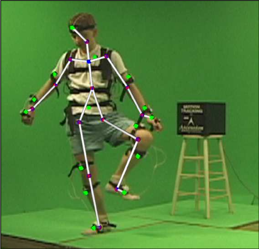
Figure 1: Test subject and generated model. The subject is wearing the motion capture equipment during a capture session; the superimposed skeletal model is generated automatically from the acquired motion capture data. The chest and pelvis sensors are located on the subject’s back.

Although motion capture has many advantages and commercial systems are improving rapidly, the technology has drawbacks. Both optical and magnetic systems suffer from sensor noise and require careful calibration[6]. Additionally, measurements such as limb lengths or the offsets between the sensors and the joints are often required. This information is usually gathered by measuring the subject in a reference pose, but hand measurement is tedious and prone to error. It is also impractical for such applications as location-based entertainment where the delay and physical contact with a technician would be unacceptable.

The algorithm described in this paper addresses the problem of calibration by automatically computing the joint locations for an articulated hierarchy from the global transformation matrices of individual bodies. We take motion data acquired with a magnetic system and determine the locations of the subject’s joints and the relative sensor locations without external measurement. The technique imposes no constraints on the sensor positions beyond those necessary for accurate capture, nor does it require the subject to pose in particular configurations. The only requirement is that the data must exercise all degrees of freedom of the joints if the technique is to return an unambiguous answer. Figure 1 shows a subject wearing magnetic motion capture sensors and the skeletal model that was generated from the motion data in an automatic fashion.

Intuitively, the algorithm proceeds by examining the sequences of transformation data generated by pairs of sensors and determining a pair of points (one in the coordinate system of each sensor) that remain collocated throughout the sequence. If the two sensors are attached to a pair of objects that are connected by a rotary joint, then a single point, the center of the joint, fulfills this criterion. Errors such as sensor noise and the fact that human joints are not perfect rotary joints, prevent an exact solution. The algorithm solves for a best-fit solution and computes the residual error that describes how well two bodies “fit” together. This metric makes it possible to infer the body hierarchy directly from the motion data by building a minimum spanning tree that treats the residuals as edge weights between the body parts.

In the following sections, we describe related work in the fields of graphics, biomechanics, and robotics, and our method for computing the joint locations from motion data. We present the results of processing human motion capture data, as well as validation results using data from a simulation and from a wooden linkage of known dimensions.

2 Background

Computer graphics researchers have explored various techniques for improving the motion capture pipeline including parameter estimation techniques such as the algorithm described in this paper. Our technique is closely related to the work of Silaghi and colleagues[18] for identifying an anatomic skeleton from optical motion capture data. With their method, the location of the joint between two attached bodies is determined by first transforming the markers on the outboard body to the inboard coordinate system. Then, for each sensor, a point that maintains an approximately constant distance from the sensor throughout the motion sequence is found. The joint location is determined from a weighted average of these points. The sensor weights are determined manually, and because the coordinate system for the inboard body is not known it must be estimated from the optical data. Our technique takes advantage of the orientation information provided by magnetic sensors. The computation is symmetric with respect to the joint between two bodies and does not require any manual processing of the data.

Inverse kinematics are often used to extract joint angles from global position data. In the animation community, for example, Bodenheimer and colleagues[2] discussed how to apply inverse kinematics in the processing of large amounts of motion capture data using a modification of a technique developed by Zhao and Badler[24]. The method presented here is not an inverse kinematics technique: inverse kinematics assumes that the dimensions of the skeleton for which joint angles are being computed is known. Our work extracts those dimensions from the motion capture data, and thus could be viewed as a preliminary step to an inverse kinematics computation.

Outside of graphics, the problem of determining a system’s kinematic parameters from the motion of the system has been studied by researchers in the fields of biomechanics[15, 16] and robotics[9]. Biomechanicists are interested in this problem because the joints play a critical role in understanding the mechanics of the human body and the dynamics of human motion. However, human joints are not ideal rotary joints and therefore do not have a fixed center of rotation. Even joints like the hip which are relatively close approximations to mechanical ball and socket joints exhibit laxity and variations due to joint loading that cause changes in the center of rotation during movement. Instead, the parameter that is often measured in biomechanics is the instantaneous center of rotation, which is defined as the point of zero velocity during infinitesimally small motions of a rigid body.

To compute the instantaneous center of rotation, biomechanicists put markers on each limb and use measurements from various configurations of the limbs. To reduce error, multiple markers are placed on each joint and a least squares fit is used to filter the redundant marker data[4]. Spiegelman and Woo proposed a method for planar motions[19], and this method was extended to general motion by Veldpaus and colleagues[22]. Their algorithm uses multiple markers on a body measured at two instants in time to establish the center of rotation.

We are primarily concerned with creating animation rather than scientific studies of human motion, and our goals therefore differ from those of researchers in the biomechanics community. In particular, because we will use the recorded motion to drive an articulated skeleton that employs only simple rotary joints, we need joint centers that are a reasonable approximation over the entire sequence of motion as opposed to an instantaneous joint center that is more accurate but describes only a single instant of motion.

The biomechanics literature also provides insight into the errors inherent in a joint estimation system and suggests an upper bound on the accuracy that we can expect. Because the joints of the human body are not perfect rotary joints, the articulated models used in animation are inherently an approximation of human kinematics. Using five male subjects with pins inserted in their tibia and femur, Lafortune and colleagues found that during a normal walk cycle the joint center of the knee compressed and pulled apart by an average of 7 mm, moved front-to-back by 14.3 mm, and side-to-side by 5.6 mm[11]. Another source of error arises because we cannot attach the markers directly to the bone. Instead, they are attached to the skin or clothing of the subject. Ronsky and Nigg reported up to 3 cm of skin movement over the tibia during ground contact in running[14].

Roboticists are also interested in similar questions because they need to calibrate physical devices. A robot may be built to precise specifications, but the nominal parameters will differ from those of the actual unit. Furthermore, because a robot is made of physical materials that are subject to deformation, additional degrees of freedom may exist in the actual unit that were not part of the design specification. Both of these differences can have a significant effect on the accuracy of the unit and compensation often requires that they be measured[9]. Taking these measurements directly can be extremely difficult so researchers have developed various automatic calibration techniques.

The calibration techniques relevant to our research infer these parameters indirectly by measuring the motion of the robot. Some of these techniques require that the robot perform specific actions such as exercising each joint in isolation[25, 13] or that it assume a particular set of configurations[10, 3], and are therefore not easily adapted for use with human performers. Other methods allow calibration from an arbitrary set of configurations but focus explicitly on the relationship between the control parameters and the end-effector. Although our technique fits into the general framework described by Karan and Vukobratović for estimating linear kinematic parameters from arbitrary motion[9], the techniques are not identical because we are interested in information about the entire body rather than only the end-effectors. In addition, we can take advantage of the position and orientation information provided by the magnetic motion sensors whereas robotic calibration methods are generally limited to the information provided by joint sensors (that may themselves be part of the set of parameters being calibrated) and position markers on the end-effector.

3 Methods

For a system of $m$ rigid bodies, let ${\cal T}^{i\rightarrow j}$ be the transformation from the $i$-th body’s coordinate system to the coordinate system of the $j$-th body ($i,j\in[0..m-1]$). The index $\omega\not\in[0..m-1]$ is used to indicate the world coordinate system so that ${\cal T}^{i\rightarrow\omega}$ is the global transformation from the $i$-th body’s coordinate system to the world coordinate system.

A transformation ${\cal T}^{i\rightarrow j}$ consists of an additive, length $3$ vector component, ${\bf t}^{i\rightarrow j}$, and a multiplicative, $3\times 3$ matrix component, ${\bf R}^{i\rightarrow j}$. We will refer to ${\bf t}^{i\rightarrow j}$ as the translational component of ${\cal T}^{i\rightarrow j}$ and to ${\bf R}^{i\rightarrow j}$ as the rotational component of ${\cal T}^{i\rightarrow j}$, although in general  ${\bf R}^{i\rightarrow j}$ may be any invertible $3\times 3$ matrix transformation.

A point, ${\bf x}^{i}$, expressed in the $i$-th coordinate system may then be transformed to the $j$-th coordinate system by

$${\bf x}^{j}={\bf R}^{i\rightarrow j}{\bf x}^{i}+{\bf t}^{i\rightarrow j}.$$ (1)

A transformation from the $i$-th coordinate system to the $j$-th coordinate system may be inverted so that given ${\cal T}^{i\rightarrow j}$, ${\cal T}^{j\rightarrow i}$ may be computed by

$${\bf R}^{j\rightarrow i} = ({\bf R}^{i\rightarrow j})^{-1}$$ (2)

$${\bf t}^{j\rightarrow i} = ({\bf R}^{i\rightarrow j})^{-1}(-{\bf t}^{i\rightarrow j}),$$ (3)

where $(\cdot)^{-1}$ indicates matrix inverse.

Because in general the bodies are in motion with respect to each other and the world coordinate system, the transformations between coordinate systems change over time. We assume that the motion data is sampled at $n$ discrete moments in time called frames, and use ${\cal T}^{i\rightarrow j}_{k}$ to refer to the value of ${\cal T}^{i\rightarrow j}$ at frame $k\in[0..n-1]$.

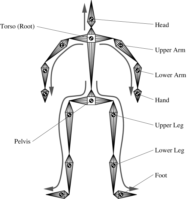
Figure 2: Example of an articulated hierarchy that could be used to model a human figure. The torso is the root body and the arrows indicate the outboard direction. For rendering, the skeleton model shown here would be replaced with a more realistic graphical model.

An articulated hierarchy is described by the topological information indicating which bodies are connected to each other and by geometric information indicating the locations of the connecting joints. The topological information takes the form of a tree with a single body located at its root and all other bodies appearing as nodes within the tree as shown in Figure 2. When referring to directions relative to the arrangement of the tree, the inboard direction is towards the root, and the outboard direction is away from the root. Thus for a joint connecting two bodies, $i$ and $j$, the parent body, $j$, is the inboard body and the child, $i$, is the outboard body. Similarly, a joint which connects a body to its parent is that body’s inboard joint and a joint connecting the body to one of its children is an outboard joint. All bodies have at most one inboard joint but may have multiple outboard joints.

The hierarchy’s topology is defined using a mapping function, $P(\cdot)$, that maps each body to its parent body so that $P(i)=j$ will imply that the $j$-th body is the immediate parent of the $i$-th body in the hierarchical tree. The object, $\tau\in[0..m-1]$, with $P(\tau)=\omega$ is the root object. To simplify discussion, we will temporarily assume that $P(\cdot)$ is known a priori. Later, in Section 3.3, we will show how $P(\cdot)$ may be inferred when only the ${\cal T}^{i\rightarrow\omega}$’s are known.

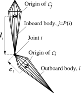
Figure 3: Joint diagram showing the location of the rotary joint between bodies $i$ and $j=P(i)$. The location of the joint is defined by a vector displacement, ${\bf c_{i}}$, relative to the coordinate system of body $i$, and a second vector displacement, ${\bf l_{i}}$, in the coordinate system of body $j$.

The geometry of the articulated hierarchy is determined by specifying the location of each joint in the coordinate frames of both its inboard body and its outboard body. Because each body has a single inboard joint, we will index the joints so that the $i$-th joint is the inboard joint of the $i$-th body as shown in Figure 3.

Let ${\bf c}_{i}$ refer to the location of the $i$-th joint in the $i$-th body’s (the joint’s outboard body) coordinate system, and let ${\bf l}_{i}$ refer to the location of the $i$-th joint in the $P(i)$-th body’s (the inboard body’s) coordinate system (see Figure 3). The transformation of equation (1) that goes from the $i$-th coordinate system to its parent’s, $P(i)$, coordinate system can then be re-expressed in terms of the joint locations, ${\bf c}_{i}$ and ${\bf l}_{i}$, and the rotation at the joint, ${\bf R}^{i\rightarrow P(i)}$, so that

$${\bf x}^{P(i)} = {\bf R}^{i\rightarrow P(i)}_{k}({\bf x}^{i}-{\bf c}_{i})+{\bf l}_{i}$$ (4)

$$= {\bf R}^{i\rightarrow P(i)}_{k}{\bf x}^{i}-{\bf R}^{i\rightarrow P(i)}_{k}{\bf c}_{i}+{\bf l}_{i}.$$ (5)

3.1 Finding Joint Locations

The general transformation given by equation (1) applies to any arbitrary hierarchy of bodies. When the bodies are connected by rotary joints, the relative motion of two connected bodies must satisfy a constraint that prevents the joint between them from coming apart. Comparing equation (5) with equation (1) shows that although rotational terms are the same, the translational term of equation (1) has been replaced with the constrained term, $-{\bf R}^{i\rightarrow P(i)}_{k}{\bf c}_{i}+{\bf l}_{i}$. Using equation (5) to transform the location of ${\bf c}_{i}$ to the $P(i)$-th coordinate system will identically yield ${\bf l}_{i}$, and equation (5) enforces the constraint that the joint stay together.

The input transformations for each of the body parts do not contain any explicit information about joint constraints. However, if the motion was created by an articulated system, then it should be possible to express the same transformations hierarchically using equation (5) and an appropriate choice of ${\bf c}_{i}$ and ${\bf l}_{i}$ for each of the joints. Thus for each pair of parent and child bodies, $i\neq\tau$ and $j=P(i)$, there should be a ${\bf c}_{i}$ and ${\bf l}_{i}$ such that equation (1) and equation (5) are equivalent and

$${\bf R}^{i\rightarrow P(i)}_{k}{\bf x}^{i}+{\bf t}^{i\rightarrow P(i)}_{k}=\\ {\bf R}^{i\rightarrow P(i)}_{k}{\bf x}^{i}-{\bf R}^{i\rightarrow P(i)}_{k}{\bf c}_{i}+{\bf l}_{i}$$ (6)

for all $k\in[0..n-1]$. After simplifying, equation (6) becomes

$${\bf t}^{i\rightarrow P(i)}_{k}=-{\bf R}^{i\rightarrow P(i)}_{k}{\bf c}_{i}+{\bf l}_{i}$$ (7)

for all $k\in[0..n-1]$. Later, it will be more convenient to work with the global transformations. By applying ${\cal T}^{P(i)\rightarrow\omega}$ to both sides of equation (7) and simplifying the result, we have

$${\bf R}^{i\rightarrow\omega}_{k}{\bf c}_{i}+{\bf t}^{i\rightarrow\omega}_{k}={\bf R}^{P(i)\rightarrow\omega}_{k}{\bf l}_{i}+{\bf t}^{P(i)\rightarrow\omega}_{k}$$ (8)

for all $k\in[0..n-1]$. Equation (8) has a consistent geometric interpretation: the location of the joint in the outboard coordinate system, ${\bf c}_{i}$, and the location of the joint in the inboard coordinate system, ${\bf l}_{i}$, should transform to the same location in the world coordinate system; in other words, the joint should stay together.

Equation (8) can be rewritten in matrix form as

$${\bf Q}^{i\rightarrow P(i)}_{k}{\bf u}_{i}={\bf d}^{i\rightarrow P(i)}_{k}.$$ (9)

where ${\bf d}^{i\rightarrow P(i)}_{k}$ is the length $3$ vector given by

$${\bf d}^{i\rightarrow P(i)}_{k}=-({\bf t}^{i\rightarrow\omega}_{k}\!-{\bf t}^{P(i)\rightarrow\omega}_{k}),$$ (10)

${\bf u}_{i}$ is the length $6$ vector

$${\bf u}_{i}=\left[\begin{array}[]{c}{\bf c}_{i}\\ {\bf l}_{i}\end{array}\right],$$ (11)

and ${\bf Q}^{i\rightarrow j}_{k}$ is the $3\times 6$ matrix

$${\bf Q}^{i\rightarrow j}_{k}=\left[({\bf R}^{i\rightarrow\omega}_{k})\;({\bf-R}^{P(i)\rightarrow\omega}_{k})\right].$$ (12)

Assembling equation (9) into a single linear system of equations for all $0..n-1$ frames gives:

$$\left[\begin{array}[]{c}{\bf Q}^{i\rightarrow P(i)}_{0}\\ \vdots\\ {\bf Q}^{i\rightarrow P(i)}_{k}\\ \vdots\\ {\bf Q}^{i\rightarrow P(i)}_{n-1}\end{array}\right]\,\left[\begin{array}[]{c}{\bf c}_{i}\\ {\bf l}_{i}\end{array}\right]=\left[\begin{array}[]{c}{\bf d}^{i\rightarrow P(i)}_{0}\\ \vdots\\ {\bf d}^{i\rightarrow P(i)}_{k}\\ \vdots\\ {\bf d}^{i\rightarrow P(i)}_{n-1}\end{array}\right].$$ (13)

The matrix of ${\bf Q}$’s is $3n\times 6$ and will be denoted by $\widehat{\bf Q}$; the matrix of ${\bf d}$’s is $3n\times 1$. The linear system of equations in equation (13) can be used to solve for the joint location parameters, ${\bf c}_{i}$ and ${\bf l}_{i}$.

Unless the input motion data consists of only two frames of motion, $\widehat{\bf Q}$ will have more rows than columns and the system will, in general, be over-constrained. Nonetheless, if the motion was generated by an articulated model, an exact solution will exist. Realistically, limited sensor precision and other sources of error will prevent an exact solution, and a best-fit solution must be found instead.

Despite the fact that the system will be over-constrained, it may be simultaneously under-constrained if the input motions do not span the space of rotations. In particular, if two bodies connected by a joint do not rotate with respect to each other, or if they do so but only about a single axis, then there will be no unique answer. In the case where they are motionless with respect to each other, any location in space would be a solution. Similarly, if their relative rotations are about a single axis, then any point on that axis could serve as the joint’s location. For reasons of numerical accuracy, in either of these cases the desired solution is chosen to be the one closest to the origin of the inboard and outboard body coordinate frames.

The technique of solving for a least squares solution using the singular value decomposition is well suited for this type of problem[17]. Because there is no numerical structure in our problem that we can exploit (such as sparsity), our use of this technique to solve equation (13) is straightforward. In later sections, we will use the residual vector from the solution of this system to show the translational difference between the input data and the value given by equation (5).

3.2 Single-axis Joints

If a joint rotates about two or more non-parallel axes, enough information is available to resolve the location of the joint center as described above. However, if the joint rotates about a single axis, then a unique joint center does not exist, and any point along the axis is an equally good solution to equation (13). In these cases the solution to equation (13) found by the singular value decomposition will be an essentially arbitrary point on the axis.

This situation can be detected by examining the singular values of $\widehat{\bf Q}$ from equation (13). If one of the singular values of $\widehat{\bf Q}$ is near zero, i.e., if $\widehat{\bf Q}$ is rank deficient, then that joint is a single-axis joint, or at least in the input motion it rotates only about a single axis. The first three components of the corresponding column vector of ${\bf V}$ from the singular value decomposition are the joint axis in the inboard coordinate frame; the second three are the axis in the outboard coordinate frame

While we were able to verify this method for detecting single-axis joints using synthetic data, none of the data from our motion capture trials indicated the presence of a single-axis joint. We believe that single-axis joints did not appear in the data because our subjects were specifically asked to exercise the full range of motion and all degrees of freedom of their joints. As a result, the system was able to determine a location even for joints such as the knee and elbow that are traditionally approximated as one degree-of-freedom joints.

3.3 Determining the Body Hierarchy

In the previous sections, we assumed that the hierarchical relationship between the bodies given by the parent function, $P(\cdot)$, is known. In some instances, however, determining a suitable hierarchy automatically by inferring it from the input transformation matrices may be desirable. Our algorithm does this by finding the parent function that minimizes the sum of the $\varepsilon_{i}$’s for all the joints in the hierarchy.

The problem of finding the optimal hierarchy is equivalent to finding a minimal spanning tree. Each body can be thought of as a node, joints are the edges between them, and the joint fit error, $\varepsilon_{i}$, is the weight of the edge. The hierarchy can then be determined by evaluating the joint error between all pairs of bodies, selecting a root node, $\tau$, and then constructing the minimal spanning tree. See [5] for example algorithms.

3.4 Removing the Residual

After we have determined the locations of the joints, we can use this information to construct a model that approximates the dimensions of the subject. This model can then be used to play back the original motion data. Unless the residual errors on the joint fits were all near zero, the motion will cause the joints of the model to move apart from each other during playback in a fashion that is typical of unconstrained motion capture data. If, however, we use the inferred joint locations to create an articulated model with kinematic joint constraints and then play back the motion through this model, the joints will stay together. Playing back motion capture data by applying only the rotations to an articulated model is common practice; the difference here is that the model itself has been generated from the motion data. Essentially, we have projected the motion data onto a parametric model and then used the fit to discard the residual.

4 Results

To verify that our algorithm could be used to determine the hierarchy and joint parameters from motion data, we tested it on both simulated data and on data acquired from a magnetic motion capture system. First, the technique was tested on a rigid-body dynamic simulation of a human containing 48 degrees of freedom. The simulated figure was moved so that all of its degrees of freedom were exercised. The algorithm correctly computed limb lengths within the limits of numerical precision (errors less than $\text{10}^{\text{-6}}$ m) and determined the correct hierarchy.

We next tested our method in a magnetic motion capture environment. Magnetic motion capture systems are frequently noisy, and the Ascension system we used has a published resolution of about 4 mm[1]. To establish a baseline for the amount of noise present in the environment, two sensors were rigidly attached 56.5 cm apart and moved through the capture space. The results of this experiment are shown in Figure 4. A scale factor exists when converting from units the motion capture system reports to centimeters, and we calculated this scale factor to be 0.94 based on the mean of this data set. The scaled standard deviation of the data is 0.7 cm.

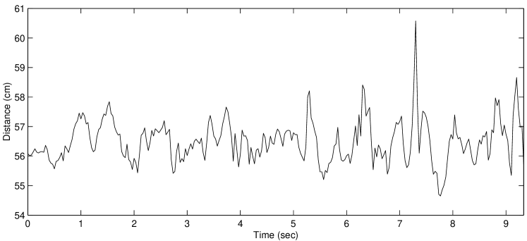
Figure 4: Calibration data showing the distance between two markers attached rigidly to one another and moved through the capture space. If the sensors are not moved, the data is much less noisy.

To test the algorithm on something less complicated than biological joints, we constructed a wooden mechanical linkage with five ball-and-socket joints. That linkage is shown in Figure 5. Six sets of data were captured in which all the degrees of freedom were exercised. Before Set 6 was captured, the marker positions were moved to evaluate the robustness of the method to changes in marker locations. The results are shown in Table 1 along with the measured values of the joint-to-joint distances. The maximum error across all trials is 1.1 cm, and the hierarchy was computed correctly for each trial. Another way of evaluating the fit is to examine the residual vectors from the least squares process. The norms of the residual vectors for the best fit (Set 1, Right Shoulder) and the worst fit (Set 6, Left Shoulder) are shown in Figures 6 and 7, respectively. The right-hand graph has an asymmetric distribution because it is the distribution of an absolute value. We regard these results as very good because the error is on the order of the resolution of the sensors.

(A) (B) (C)

Figure 5: Wooden mechanical linkage. (A) Labels indicate the terms that we used to refer to the body parts; circles highlight the joint locations. (B) The motion capture sensors (highlighted squares) have been attached to the linkage. (C) The model computed automatically from the motion data using our algorithm. The joints are shown with spheres, and the sensors with cubes. Links between joints are indicated with cylinders.

	Meas.	Set 1	Set 2	Set 3	Set 4	Set 5	Set 6	$\Delta$ 1	$\Delta$ 2	$\Delta$ 3	$\Delta$ 4	$\Delta$ 5	$\Delta$ 6
Neck — Left Shoulder	39.0	39.4	38.8	39.8	39.1	39.1	40.1	-0.4	-0.2	-0.8	-0.1	-0.1	-1.1
Neck — Right Shoulder	39.7	39.8	39.8	40.3	40.0	39.9	40.3	-0.1	-0.1	-0.6	-0.3	-0.2	-0.6
Between Shoulders	34.3	34.3	33.7	34.5	34.3	34.3	34.8	-0.0	-0.6	-0.2	-0.0	-0.0	-0.5
Right Upper Arm	28.6	29.2	29.0	28.8	28.9	29.0	29.1	-0.6	-0.4	-0.2	-0.3	-0.4	-0.5
Left Upper Arm	31.4	31.5	31.7	31.9	31.5	31.1	31.2	-0.1	-0.3	-0.5	-0.1	-0.3	-0.2

Table 1: A comparison of measurements and calculated limb lengths for six data sets of the mechanical linkage. The units are centimeters and the columns labeled $\Delta$ show the difference in measured and calculated values. Joint names follow the analogy with human physiology used in Figure 5(A).

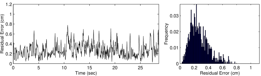
Figure 6: Residual errors of the right shoulder joint for the data from Set 1 for the mechanical linkage (Table 1). The left graph shows the magnitude of the residual vector. The right graph shows the distribution of the frequency of the magnitudes.

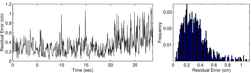
Figure 7: Residual errors of the left shoulder joint for the data from Set 6 for the mechanical linkage (Table 1).

The important test case, of course, is to verify that we are able to estimate the limb lengths of people. This task is more difficult because human joints are not simple mechanical linkages. To provide a basis for comparison, we measured the limb lengths of our test subjects. As mentioned previously, this process is inexact and prone to error, but it does provide a plausible estimate. We measured limb lengths from bony landmark to bony landmark to provide repeatability and consistency in our measurements. For example, the upper leg of a subject was measured as the distance from the top of the greater trochanter of the femur to the lateral condyle of the tibia. Because the head of the femur extends upward and inward into the innominate, this measurement will be inaccurate by a few centimeters. Nonetheless, because the greater trochanter is the only palpable area at the upper end of the femur, this measurement is the best available. The difficulty in obtaining accurate hand measurements is one of the primary reasons that we chose to develop our automatic technique.

Our test subjects performed two different sets of motions for capture. We refer to the first set as the “exercise” set. In it the subjects attempted to move each joint essentially in isolation to generate a full range of motion for each joint. Thus the routine consists of a set of discrete motions such as rolling the head around on the neck, bending at the waist, high-stepping, lifting each leg and waving it about, lifting the arms and waving them about, bending the elbows and the wrists, etc. This exercise set mimics the way we gathered data for the mechanical linkage. We refer to the second set of motions captured as the “walk” sets. In it the subjects try to move as many degrees of freedom at once as they can while walking. This routine is perhaps best described as a “chicken” walk, consisting of highly exaggerated leg movements coupled with bending the waist and waving the arms about.

A male subject performed the two types of motion and the results of the limb length calculations are shown in Tables 4 and 4. As expected, the residual errors for a human are much larger than for the mechanical linkage. A representative example is shown in Figure 8. For this subject, the maximum difference between measured and calculated values is 4.1 cm, and occurs at the left upper arm during one of the exercise sets. The mean of the differences between calculated and measured values is less than one centimeter for every limb except the upper arms where it is 1.4 cm and 2.2 cm for the right and left arms, respectively. The algorithm consistently finds a longer length for the left upper arm than what we measured, and that difference may be due, in part, to an error in the value measured by hand. However, the shoulder joint is poorly approximated by a rotary joint: an accurate biomechanical rigid-body model would have at least seven degrees of freedom[21, 20], and it is not surprising that the worst fit occurs there.

The same motions were repeated with a female subject, and the results are shown in Table 4. The largest difference between calculated and measured values is 2.4 cm and again occurs for the left upper arm. The algorithm also finds a longer length for the left upper arm than we measured. The maximum error is less than that for the male test subject, but less consistency was found among the results for the female test subject. The mean of the differences between the calculated and measured values is greater than one centimeter for the right lower leg, left upper leg, and left upper arm.

The system also computed a hierarchy for each trial. For all “exercise” trials for both male and female subjects the computed hierarchy was correct; however, results from the “walk” data were less satisfactory. For three of the five “walk” trials, the algorithm improperly made one of the upper legs a child of the other instead of the pelvis. This error may have occurred because the pelvis sensor was mounted on the system’s battery pack worn on the subject’s hip. Motion in this sensor caused by rotating the thigh upwards may have contributed to the error. The limb length results we report are, of course, for the correct hierarchy assignments.

In addition to the joint measurements we reported, our algorithm determines information for joints (such as between the chest and pelvis) that model the bending of the torso but which are gross approximations to the way the human spine bends. Our algorithm reports limb lengths for these joints within the torso, and these are generally consistent with the dimensions of the torsos of the subjects. However, because we have no reasonable way of measuring these lengths for comparison, we have omitted them from the results. The locations computed for these joints can be seen in Figure 1 and in the animations that accompany this paper.

The algorithm is quite fast. On an SGI O2 with a 195 MHz R10000 processor, less than 4 seconds are required to process 45 seconds of motion data for 16 sensors with the hierarchy specified, and less than 14 seconds when the hierarchy was not specified.

	Meas.	Exer. 1	Exer. 2	Exer. 3	Exer. 4	$\Delta$ 1	$\Delta$ 2	$\Delta$ 3	$\Delta$ 4
Right Lower Leg	40.0	40.8	40.9	42.2	42.5	-0.8	-0.9	-2.2	-2.5
Left Lower Leg	40.3	37.3	38.4	41.2	41.5	-3.0	-1.9	-0.9	-1.2
Right Upper Leg	41.6	41.5	42.1	42.9	42.2	-0.1	-0.5	-1.3	-0.6
Left Upper Leg	43.2	41.4	41.8	43.2	43.0	-1.8	-1.4	-0.0	-0.2
Right Lower Arm	27.0	26.3	26.7	27.7	27.0	-0.7	-0.3	-0.7	-0.0
Left Lower Arm	26.7	26.5	27.0	26.7	27.1	-0.1	-0.3	-0.1	-0.4
Right Upper Arm	29.5	32.1	31.3	29.3	28.8	-2.6	-1.8	-0.2	-0.7
Left Upper Arm	29.5	33.7	32.9	30.1	29.9	-4.1	-3.4	-0.6	-0.4

Table 2: A comparison of measurements and calculated limb lengths for four data sets of a male subject attempting to exercise each degree of freedom essentially in isolation.

	Meas.	Walk 1	Walk 2	Walk 3	$\Delta$ 1	$\Delta$ 2	$\Delta$ 3
Right Lower Leg	40.0	40.7	40.3	38.9	-0.6	-0.3	-1.1
Left Lower Leg	40.3	40.8	38.9	39.8	-0.4	-1.4	-0.5
Right Upper Leg	41.6	40.7	40.6	42.6	-0.9	-1.0	-1.0
Left Upper Leg	43.2	45.1	42.7	43.1	-1.9	-0.5	-0.1
Right Lower Arm	27.0	27.3	27.5	25.8	-0.3	-0.5	-1.2
Left Lower Arm	26.7	26.2	24.9	25.6	-0.5	-1.7	-1.0
Right Upper Arm	29.5	31	31.1	32.7	-1.4	-1.6	-3.2
Left Upper Arm	29.5	32.3	32.3	30.8	-2.7	-2.7	-1.3

Table 3: A comparison of measurements and calculated limb lengths for three data sets of a male subject attempting to exercise all degrees of freedom simultaneously.

	Meas.	Exer. 1	Walk 1	Walk 2	$\Delta_{e}$ 1	$\Delta_{w}$ 1	$\Delta_{w}$ 2
Right Lower Leg	36.8	39.1	38.0	38.1	-2.3	-1.2	-1.3
Left Lower Leg	36.5	37.6	37.0	37.4	-1.1	-0.5	-0.9
Right Upper Leg	42.2	42.9	43.3	42.2	-0.7	-1.1	-0.0
Left Upper Leg	41.9	42.4	44.1	42.9	-0.5	-2.2	-1.0
Right Lower Arm	24.8	25.5	25.3	22.4	-0.7	-0.5	-2.3
Left Lower Arm	24.8	25.1	24.8	23.0	-0.3	-0.0	-1.8
Right Upper Arm	27.6	27.5	27.5	28.7	-0.2	-0.1	-1.0
Left Upper Arm	27.6	28.5	30.0	29.0	-0.9	-2.4	-1.3

Table 4: A comparison of measurements and calculated limb lengths for four data sets of a female subject. The column labeled “Exercise” denotes a performance attempting to exercise each degree of freedom in isolation. Columns labeled “Walk” denote a performance attempting to exercise all degrees of freedom simultaneously. The units are centimeters, and the columns labeled $\Delta$ show the difference in measured and calculated values for the appropriate set.

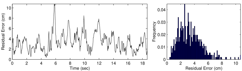
Figure 8: Residual errors of the left shoulder for the data from Walk 2 of a male subject (Table 4). The scale of the residual vectors is larger than that of the residual vectors for Figures 6 and 7.

5 Discussion and Conclusions

This paper presents an automatic method for computing limb lengths, joint locations, and sensor placement from magnetic motion capture data. The method produces results accurate to the resolution of the sensors for data that was recorded from a mechanical device constructed with rotary joints. The accuracy of the results for data recorded from a human subject is consistent with estimates in the biomechanics literature for the error introduced by approximating human joints as rotational and assuming that the skin does not move with respect to the bone.

Measuring and calibrating a performer in a production animation environment is tedious. Because this algorithm runs very quickly, it provides a rapid way to accomplish the calibration for magnetic motion capture systems. Detecting and correcting for marker slippage are additional complications in the motion capture pipeline. Because this technique looks for large changes in the joint residual, it provides a rapid way of determining if a marker slipped during a particular recorded segment, thus allowing the segment to be performed again while the subject is still suited with sensors.

The parameters computed by this method can be used to create a digital version of a particular performer by matching a graphical model to the proportions of the motion capture subject. The process does not require the subject to assume a particular pose or to perform specific actions other than to exercise their joints fully. Therefore, the method can be incorporated into applications where explicit calibration is infeasible. A cleverly disguised “exercise” routine, for example, could be part of the pre-show portion of a location-based entertainment experience.

The algorithm would also be of use in applications where the problem is fitting data to a graphical model with dimensions different from those of the motion capture subject. The algorithm presented here could be used in a pre-processing step to provide the best-fit limb lengths for the data and modify the data to have constant limb lengths. Then constraint-based techniques could be applied to adapt the resulting motion to the new dimensions of the graphical character.

Passive optical systems often have problems with marker identification because occlusion causes markers to appear to swap. For example, when the hand passes in front of the hip during walking, the marker on the hand and the one on the hip may become confused. If this happens, the marker locations may change relatively smoothly but the joint center of the inboard and outboard bodies for each marker will change discontinuously. This error should be identifiable when the data is processed, allowing the markers to be disambiguated.

For relatively clean data, this algorithm can be used to extract the hierarchy automatically. Specifying the hierarchy is not burdensome for magnetic motion capture data because the markers are uniquely identified by the system. However, automatic identification of the hierarchy might be useful in situations where connections between objects are dynamic such as pairs dancing or a subject manipulating an instrumented object.

We have assumed that the hierarchy is a strict tree and does not contain cycles or loop joints such as the closed chain that is created when the hands are clasped. If the hierarchy is known a priori, the location of a loop joint is found just as it is for any other joint. If the hierarchy is not known, the method of Section 3.3 will not find cycles and the hierarchy it returns will be missing the additional joints required to close the loops. This problem could be detected by informing the user that a joint fit with a low error was not used in building the tree.

The algorithm we have described is statistically equivalent to fitting a parameterized model to a distribution. The rotary joint model that is commonly used for skeletal animation is linear, but more complex models that explicitly model the errors introduced by the non-rotational nature of the joints, the slippage of skin, or the noise distribution seen in the magnetic setup would be non-linear. Non-linear models have been used in robotics research to model elastic deformation of robot limb segments, joints that do not have a fixed center of rotation, and dynamic variation due to system inertial properties[12, 7, 23, 8, 9]. Reconstructing the motion based on the joint locations, as described in Section 3.4, is a first step towards identifying the components of the motion that are due to actual motion and those that are due to errors. The addition of more sophisticated models could allow us to separate components of the data attributable to the motion of the subject from components that are due to other sources. This separation might allow accurate data to emerge even from systems where the sensors are only loosely attached to the subject.

- [1] Ascension Technology Corporation, http://www.ascension-tech.com.
- [2] B. Bodenheimer, C. Rose, S. Rosenthal, and J. Pella. The process of motion capture: Dealing with the data. In D. Thalmann and M. van de Panne, editors, Computer Animation and Simulation ’97, pages 3–18. Springer NY, Sept. 1997. Eurographics Animation Workshop.
- [3] J.-H. Borm and C.-H. Menq. Experimental study of observability of parameter errors in robot calibration. In Proceeding of the 1989 IEEE International Conference on Robotics and Automation, pages 587–592. IEEE Robotics and Automation Society, 1998.
- [4] J. H. Challis. A procedure for determining rigid body transformation parameters. Journal of Biomechanics, 28(6):733–737, 1995.
- [5] T. H. Cormen, C. E. Leiserson, and R. L. Rivest. Introduction to Algorithms. McGraw–Hill Book Company, fourth edition, 1991.
- [6] B. Delaney. On the trail of the shadow woman: The mystery of motion capture. IEEE: Computer Graphics and Applications, 18(5):14–19, 1998.
- [7] A. A. Goldenberg, X. He, and S. P. Ananthanarayanan. Identification of inertial parameters of a manipulator with closed kinematic chains. IEEE: Transactions on Systems, Man, and Cybernetics, 22(4):799–805, 1992.
- [8] R. Gourdeau, G. M. Cloutier, and J. Laflamme. Parameter identification of a semi-flexible kinematic model for serial manipulators. Robotica, 14:331–319, 1996.
- [9] B. Karan and M. Vukobratović. Calibration and accuracy of manipulation robot models – an overview. Mechanism and Machine Theory, 29(3):479–500, 1992.
- [10] D. H. Kim, K. H. Cook, and J. H. Oh. Identification and compensation of robot kinematic parameters for positioning accuracy improvement. Robotica, 9:99–105, 1991.
- [11] M. A. Lafortune, P. R. Cavanaugh, H. J. Sommer, and A. Kalenka. Three-dimensional kinematics of the human knee during walking. Journal of Biomechanics, 25(4):347–357, Apr. 1992.
- [12] J. Lai and H. X. Lan. Identification of dynamic parameters in lagrange robot model. In Proceedings of 1988 IEEE International Conference on Systems, Man, and Cybernetics, pages 90–93, 1988.
- [13] R. Liscano, H. El-Zorkany, and I. Mufti. Identification of the kinematic parameters of an industrial robot. In Proceedings of COMPINT ’85: Computer Aided Technologies, pages 477–480, Montreal, Quebec, Canada, 1985. National Research Council of Canada, IEEE Computer Society Press. Held in Montreal, Quebec, Canada, 8–12 September 1985.
- [14] B. M. Nigg and W. Herzog, editors. Biomechanics of the Musculo-skeletal system. John Wiley, New York, 1998.
- [15] M. M. Panjabi, V. K. Goel, and S. D. Walter. Errors in kinematic parameters of a planar joint: Guidelines for optimal experimental design. Journal of Biomechanics, 15(7):537–544, 1982.
- [16] M. M. Panjabi, V. K. Goel, S. D. Walter, and S. Schick. Errors in the center and angle of rotation of a joint: An experimental study. Journal of Biomechanical Engineering, 104:232–237, Aug. 1982.
- [17] W. H. Press, B. P. Flannery, S. A. Teukolsky, and W. T. Vetterling. Numerical Recipes in C. Cambridge University Press, second edition, 1994.
- [18] M.-C. Silaghi, R. Plänkers, R. Boulic, P. Fua, and D. Thalmann. Local and global skeleton fitting techniques for optical motion capture. In N. Magnenat-Thalmann and D. Thalmann, editors, Modelling and Motion Capture Techniques for Virtual Environments, volume 1537 of Lecture Notes in Artificial Intelligence, pages 26–40, Berlin, Nov. 1998. Springer. Proceedings of CAPTECH ’98.
- [19] J. J. Spiegelman and S. L.-Y. Woo. A rigid-body method for finding centers of rotation and angular displacements of planar joint motion. Journal of Biomechanics, 20(7):715–721, 1987.
- [20] F. C. T. van der Helm. Analysis of the kinematic and dynamic behavior of the shoulder mechanism. Journal of Biomechanics, 27(5):527–550, May 1994.
- [21] F. C. T. van der Helm. A finite element musculoskeletal model of the shoulder mechanism. Journal of Biomechanics, 27(5):551–569, May 1994.
- [22] F. E. Veldpaus, H. J. Woltring, and L. J. M. G. Dortmans. A least-squares algorithm for the equiform transformation from spatial marker co-ordinates. Journal of Biomechanics, 21(1):45–54, 1988.
- [23] D. W. Williams and D. A. Turcic. An inverse kinematic analysis procedure for flexible open-loop mechanisms. Mechanism and Machine Theory, 27(6):701–714, 1992.
- [24] J. Zhao and N. Badler. Inverse kinematics positioning using nonlinear programming for highly articulated figures. ACM Transactions on Graphics, 13(4):313–336, 1994.
- [25] H. Zhuang and Z. S. Roth. A linear solution to the kinematic parameter identification of robot manipulators. IEEE: Transactions on Robotics and Automation, 9(2):174–185, 1993.