Random site percolation thresholds on square lattice for complex neighborhoods containing sites up to the sixth coordination zone

Abstract

The site percolation problem is one of the core topics in statistical physics. Evaluation of the percolation threshold, which separates two phases (sometimes described as conducting and insulating), is useful for a range of problems from core condensed matter to interdisciplinary application of statistical physics in epidemiology or other transportation or connectivity problems. In this paper with Newman–Ziff fast Monte Carlo algorithm and finite-size scaling theory the random site percolation thresholds $p_{c}$ for a square lattice with complex neighborhoods containing sites from the sixth coordination zone are computed. Complex neighborhoods are those that contain sites from various coordination zones (which are not necessarily compact). We also present the source codes of the appropriate procedures (written in C) to be replaced in original Newman–Ziff code. Similar to results previously found for the honeycomb lattice, the percolation thresholds for complex neighborhoods on a square lattice follow the power law $p_{c}(\zeta)\propto\zeta^{-\gamma_{2}}$ with $\gamma_{2}=0.5454(60)$, where $\zeta=\sum_{i}z_{i}r_{i}$ is the weighted distance of sites in complex neighborhoods ($r_{i}$ and $z_{i}$ are the distance from the central site and the number of sites in the coordination zone $i$, respectively).

I Introduction

Percolation Broadbent and Hammersley (1957); Hammersley (1957) is one of the core problems in statistical physics with many interdisciplinary applications ranging from materials science Cheng et al. (2020), through studies of polymer composites Zhang et al. (2020), forest fires Malarz et al. (2002), agriculture Ramírez et al. (2020), oil and gas exploration Ghanbarian et al. (2020), diseases propagation Ziff (2021), transportation networks Dong et al. (2020), quantifying urban areas Cao et al. (2020), to Bitcoins transfer Bartolucci et al. (2020) (see References Li et al., 2021; Saberi, 2015 for reviews). The percolating system undergoes a (purely geometrical) phase transition (in terms of the conductivity or transportation properties of the system) from the phase corresponding to an insulator (for low connectivity $p<p_{c}$) to a conductor (for high connectivity $p>p_{c}$). The critical connectivity of the system $p_{c}$ (called the percolation threshold) separates these two phases and depends on the dimension of the system $d$, the topology of the lattice, the number $z$ of sites in the assumed neighborhood, the type of percolation (that is, the site or bond dilution), etc. Stauffer and Aharony (1994); Wierman (2014).

Percolation thresholds were initially estimated for nearest-neighbor interactions Dean (1963); Dean and Bird (1967); Suding and Ziff (1999) but later also complex neighborhoods (termed also extended for compact neighborhoods) were studied for various lattices embedded in:

• $d=2$ (for a square Dalton et al. (1964); Domb and Dalton (1966); Gouker and Family (1983); Malarz and Galam (2005); Galam and Malarz (2005); Majewski and Malarz (2007); Xun et al. (2021), a triangular Dalton et al. (1964); Domb and Dalton (1966); d’Iribarne et al. (1999); Malarz (2020, 2021), a honeycomb Dalton et al. (1964); Malarz (2022) and other Archimedean Lebrecht et al. (2021); Xun et al. (2022) lattices);

• $d=3$ (for a simple cubic Kurzawski and Malarz (2012); Malarz (2015); Xun et al. (2021) lattice);

• $d=4$ (for a simple hypercubic Kotwica et al. (2019); Zhao et al. (2022) lattice)

dimensions.

(a)

(b)

(c)

(d)

(e)

(f)

Figure 1: Shapes of basic neighborhoods on square lattice. 1(a) sq-1, $r^{2}=1$, 1(b) sq-2, $r^{2}=2$, 1(c) sq-3, $r^{2}=4$, 1(d) sq-4, $r^{2}=5$, 1(e) sq-5, $r^{2}=8$, 1(f) sq-6, $r^{2}=9$. The number $r$ is the radius of (orange) circle indicating equidistant sites marked by solid (black) circles to the central one marked with open (red) circle

Simultaneously with the estimation of percolation thresholds for various lattices, some effort went into searching for an analytical formula allowing for the prediction of the percolation threshold position based on lattice characteristics. For example, Xun et al. Xun et al. (2022) estimated the site and bond percolation thresholds for 11 Archimedean lattices with complex and compact (extended) neighborhoods containing sites up to the tenth coordination zone. For the site percolation problem, the critical site occupation probability $p_{c}$ follows asymptotically

$$p_{c}(z)=a/z$$ (1)

with the total number $z$ of sites in the neighborhood and $a\approx 4.51235$. This dependence should be reached exactly for the percolation of compact neighborhoods with a large number $z$ of sites that make up the neighborhood (for example, for discs). To take into account finite-$z$ effect an additional term $b$ in the denominator of Equation 1

$$p_{c}(z)=c/(z+b)$$ (2)

has been included Xu et al. (2021). For the two-dimensional lattices $b=3$ Xun et al. (2022). The third universal scaling studied in by Xun et al. Xun et al. (2022) was

$$p_{c}(z;d)=1-\exp(d/z)$$ (3)

proposed by Koza et al. Koza et al. (2014); Koza and Poła (2016).

Much earlier Galam and Mauger Galam and Mauger (1996, 1997) proposed a universal formula for site percolation problem

$$p_{c}(z;d)=\dfrac{p_{0}}{[(d-1)(z-1)]^{a}}.$$ (4)

They recognized two classes of systems (two sets of $(p_{0},a)$ parameters) Galam and Mauger (1996). Their paper Galam and Mauger (1996) was immediately criticized by van der Marck van der Marck (1997) who showed ‘an example of two networks, where $d$ and $z$ are equal, but the percolation thresholds differ’.

For complex neighborhoods, the situation is even more complex, since for a given lattice topology (and thus fixed $d$) there are many neighborhoods with exactly the same total number $z$ of sites in the neighborhood but different percolation thresholds $p_{c}$ (see: Table 1 and Figure 4 in Reference Majewski and Malarz, 2007 for the square lattice; Table 1 in Reference Malarz, 2020 and Table 1 and Figure 3(a) in Reference Malarz, 2021 for the triangular lattice; and Table 1 and Figure 4(a) in Reference Malarz, 2022 for the honeycomb lattice).

To solve the above-mentioned problems of $p_{c}(z)$ degeneration the index

$$\xi=\sum_{i}z_{i}r_{i}^{2}/i$$ (5)

was proposed by Malarz Malarz (2021). The $z_{i}$ and $r_{i}$ are the number of sites and their distance from the central site in the neighborhood in the $i$-th coordination zone. The index $\xi$ allowed for a successful distinguishing between neighborhoods and cancel $p_{c}(z)$ degeneration for the triangular lattice with complex neighborhoods containing sites up to the fifth coordination zone. The dependence of the percolation threshold

$$p_{c}(\xi)\propto\xi^{-\gamma_{1}}$$ (6)

was well fitted with the power law with $\gamma_{1}(\textsc{tr})\approx 0.710(19)$. Unfortunately, this dependence does not hold for the honeycomb lattice (see Figure 4(b) in Reference Malarz, 2022). Thus, another index

$$\zeta=\sum_{i}z_{i}r_{i}$$ (7)

was introduced by Malarz, to simultaneously resolve the problem of $p_{c}(z)$ degeneration and to distinguish among various complex neighborhoods for the honeycomb lattice Malarz (2022). For honeycomb lattice and complex neighborhoods up to the fifth coordination zone

$$p_{c}(\zeta)\propto\zeta^{-\gamma_{2}}$$ (8)

with $\gamma_{2}(\textsc{hc})\approx 0.4981(90)$ Malarz (2022).

In this paper, using the fast Monte Carlo Newman–Ziff algorithm Newman and Ziff (2001), we calculate the critical occupation probabilities $p_{c}$ (percolation thresholds) for random site percolation in a square lattice and neighborhoods combined with basic neighborhoods presented in Figure 1. The basic neighborhoods contain sites from the first coordination zone (sq-1, Figure 1(a)) up to the sixth coordination zone (sq-6, Figure 1(f)). These complex neighborhoods are presented in Figure 4 in Appendix A. Calculations of percolation thresholds are based on the finite-size scaling hypothesis Privman (1990); Stauffer and Aharony (1994); Landau and Binder (2009).

The second aim of this paper is to check if Equations 6 and 8 holds for a square lattice with complex neighborhoods and, if so, which of them performs better.

The rest of the paper is organized as follows. The details of the calculations are presented in the following Section II. The results of the calculations are given in Section III. The article is summarized and concluded in Section V. The Appendix A contains graphical presentation of neighborhood shapes. In “Supplementary materials” we present:

• a set of boundaries() functions (written in C, Listings 1 to 6) to be replaced in the Newman–Ziff program published in Reference Newman and Ziff, 2001 to obtain the single realization of $\mathcal{S}_{\max}(n;L)$ for the neighborhoods presented in Figures 1(a), 1(b), 1(c), 1(d), 1(e) and 1(f);

• and the dependencies of $\mathcal{P}_{\max}\cdot L^{\beta/\nu}$ on the probability of occupation $p$ for neighborhoods ranging from sq-6 to sq-1,2,3,4,5,6 for various linear system sizes $L=128$ to 4096.

II Computations

Our calculations of the percolation thresholds $p_{c}$ are based on finite-size analyses of the probability $\mathcal{P}_{\text{max}}$ that the randomly selected site belongs to the largest cluster of occupied sites. According to the finite-size hypothesis Privman (1990); Stauffer and Aharony (1994); Landau and Binder (2009), in the vicinity of a phase transition (marked by a critical point $x_{c}$), many quantity $\mathcal{A}$ characterizing the system obeys a scaling relation

$$\mathcal{A}(x;L)=L^{-\varepsilon_{1}}\mathcal{F}\left((x-x_{c})L^{\varepsilon_{2}}\right),$$ (9)

where $x$ measures the level of system disorder (temperature for the Ising or Potts model, site/bond occupation probability for percolation problem), $L$ is the linear size of the system, $\mathcal{F}$ is a scaling function (usually analytically unknown) and $\varepsilon_{1}$ and $\varepsilon_{2}$ are scaling exponents. In other words, there exists a function $\mathcal{F}$, that for properly assumed values of $x_{c}$, $\varepsilon_{1}$ and $\varepsilon_{2}$ the dependencies of $\mathcal{A}(x)$ collapse into a single curve independently of the (finite) system size $L$. This also provides an elegant way to predict the value of the critical parameter $x_{c}$ as

$$\mathcal{A}(x;L)L^{\varepsilon_{1}}=\mathcal{F}\left((x-x_{c})L^{\varepsilon_{2}}\right),$$ (10)

which for $x=x_{c}$ yields

$$\mathcal{A}(x_{c};L)L^{\varepsilon_{1}}=\mathcal{F}\left(0\right).$$ (11)

In other words, we expect the curves $L^{\varepsilon_{1}}\mathcal{A}(x)$ plotted for various sizes of linear systems $L$ to intercept each other at $x=x_{c}$.

For our purposes, we assume that $\mathcal{A}\equiv\mathcal{P}_{\text{max}}$ (the probability that a randomly selected site belongs to the largest cluster) and $x\equiv p$ (the probability of occupation of the sites). For the problem of site percolation, the critical values of the exponents $\varepsilon_{1}$ and $\varepsilon_{2}$ are known exactly (Stauffer and Aharony, 1994, p. 54) as $\varepsilon_{1}=\frac{5}{36}/\frac{4}{3}=\frac{5}{48}$ and $\varepsilon_{2}=1/\frac{4}{3}=\frac{3}{4}$.

To compute the probability of belonging to the largest cluster

$$\mathcal{P}_{\max}(p;L)=\mathcal{S}_{\text{max}}(p;L)/N$$ (12)

we first need to calculate the sizes of the largest cluster $S_{\text{max}}$ and $N=L^{2}$ is the number of all sites available in the system.

To that end, we use three concepts presented in Reference Newman and Ziff, 2001.

• The first is the fast system construction scheme (known as the Newman–Ziff algorithm). The efficiency of this approach is based on the recursive construction of the system with $n$ occupied sites with the addition of only one occupied site to the system containing $(n-1)$ already occupied sites.

• The second concept is the way of transforming the $\bar{\mathcal{A}}(n;N)$ dependence on the integer number of occupied sites $n$ into the dependence $\mathcal{A}(p;N)$ on the probability of the site occupation $p$

  $$\mathcal{A}(p;N)=\sum_{n=0}^{N}\bar{\mathcal{A}}(n;N)\mathcal{B}(n;N,p),$$ (13)

  where

  $$\mathcal{B}(n;N,p)=\binom{N}{n}p^{n}(1-p)^{N-n}$$ (14)

  are values of the binomial (Bernoulli) probability distribution.

• The third concept is the efficient construction of the binomial coefficients (14).

The applied scheme defined in Equation 13 together with the construction of the binomial distribution coefficients is presented in Algorithm 1.

Algorithm 1 Conversion $\bar{\mathcal{A}}(n)$ to $\mathcal{A}(p)$ Newman and Ziff (2001)

1:$p_{1}$, $p_{2}$, $\Delta p$, $N$, $\bar{\mathcal{A}}(n)$ $\triangleright$ $n\in\{0,1,\cdots,N-1,N\}$

2:$\mathcal{A}(p)$ $\triangleright$ for $p$ from $p_{1}$ to $p_{2}$ every $\Delta p$

3:$p\leftarrow p_{1}$

4:while $p\leq p_{2}$ do

5:     $n_{\text{max}}=pN$ $\triangleright$ store $\mathcal{B}(N,n,p)$ to $\hat{B}$

6:     $B(n_{\text{max}})=pN$

7:     for $n=n_{\text{max}}+1,N$ do

8:         $B(n)=B(n-1)\cdot\dfrac{(N-n+1)p}{n(1-p)}$

9:     end for

10:     for $n=n_{\text{max}}-1,0,-1$ do

11:         $B(n)=B(n+1)\cdot\dfrac{(n+1)(1-p)}{p(N-n)}$

12:     end for

13:     $c\leftarrow\sum\hat{B}$

14:     $\hat{B}\leftarrow\hat{B}/c$

15:     $\mathcal{A}(p)=0$

16:     for all $n$ do

17:         $\mathcal{A}(p)\leftarrow\mathcal{A}(p)+B(n)\bar{\mathcal{A}}(n)$

18:     end for

19:     return $p,\mathcal{A}(p)$

20:     $p\leftarrow p+\Delta p$

21:end while

III Results

In Figure 2 examples of the results (for neighborhood sq-1,2,3,4,5,6 and various sizes of linear systems $L=128$, 256, 512, 1024, 2048, and 4096) of the computations obtained with the procedure described in Section II are presented. Figure 2(a) shows dependencies of the largest cluster size $\mathcal{S}_{\text{max}}$ (normalized to the system size $L^{2}$) vs. the number of occupied sites $n$ (also normalized to the system size $L^{2}$). With increasing system linear size $L$ the dependence $\mathcal{S}_{\text{max}}(n)$ becomes steeper and steeper. Figure 2(b) shows $L^{\varepsilon_{1}}\mathcal{P}_{\text{max}}(p)$ for $p$ ranging from 0.134 to 0.152 estimated for every $\Delta p=10^{-4}$. Figure 2(c) shows close-up of Figure 2(b) in the vicinity of the percolation threshold (for $p$ from 0.1430 to 0.1435 for every $\Delta p=10^{-5}$). The finite-size effects in $L^{\varepsilon_{1}}\mathcal{P}_{\text{max}}(p)$ vanish for $p=p_{c}$, resulting in a common point of $L^{\varepsilon_{1}}\mathcal{P}_{\text{max}}(p)$ plotted for various linear sizes $L$ of the systems. The analogous dependencies for all other complex neighborhoods—presented in Figure 4 in Appendix A—containing sites from the sixth coordination zone are shown in Figure 5. The results are averaged over the realizations of the $R=10^{5}$ system. The obtained $p_{c}$ are gathered in Table 1.

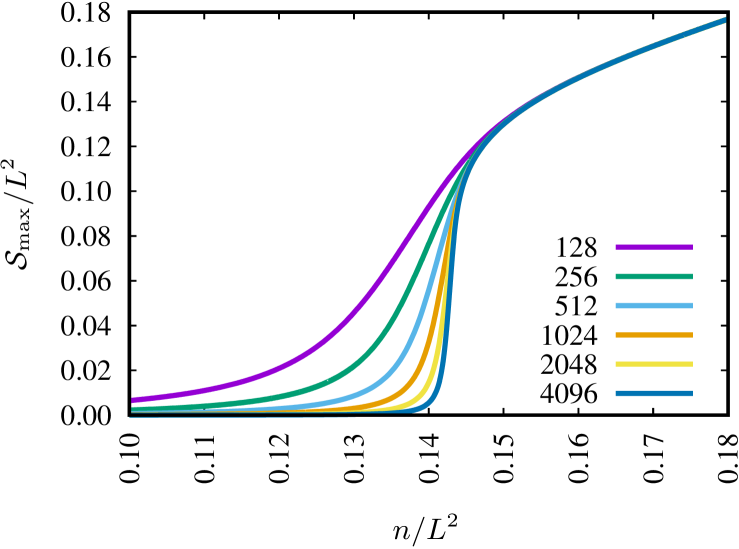
(a)

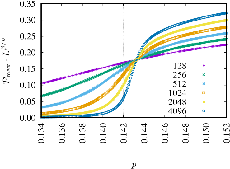
(b)

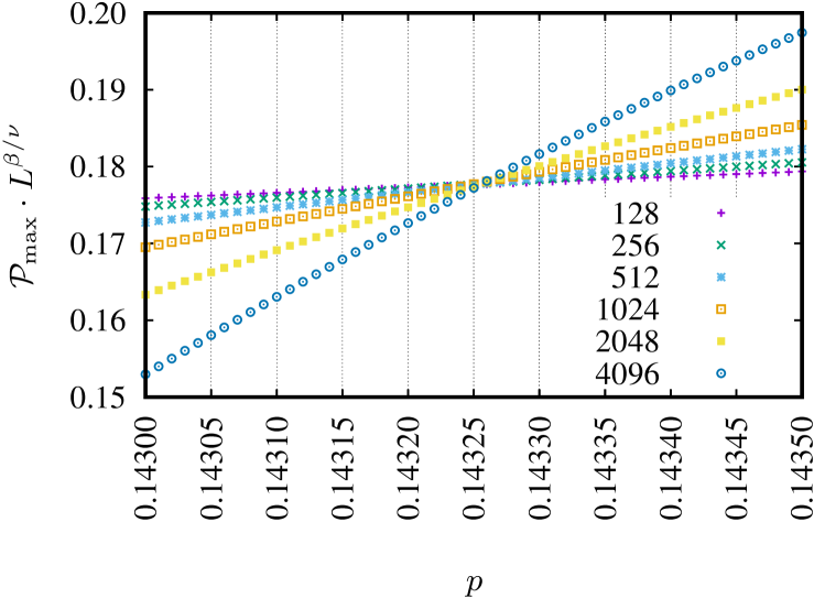
(c)

Figure 2: An example of results obtained for sq-1,2,3,4,5,6 neighborhood and various linear system sizes $L=128$ to 4096. 2(a) The size of the largest cluster $\mathcal{S}_{\text{max}}$ vs. the number of occupied sites $n$. Both quantities are normalized to the system size $L^{2}$. 2(b) Dependence of $L^{\varepsilon_{1}}\mathcal{P}_{\text{max}}(p)$ for $p$ from 0.134 to 0.152 every $\Delta p=10^{-4}$. 2(c) Close-up on Figure 2(b) in the vicinity of the percolation threshold $p_{c}$ for $p$ from 0.1430 to 0.1435 every $\Delta p=10^{-5}$

Table 1: Percolation thresholds $p_{c}$ for a square lattice with complex neighborhoods (and their characteristics $z$, $\zeta$, $\xi$) containing sites from the sixth coordination zone

lattice	z	ζ	ξ	p_c
sq-1,2,3,4,5,6	$28$	$58.8591$	$35.7333$	$0.14326$
sq-2,3,4,5,6	$24$	$54.8591$	$31.7333$	$0.14575$
sq-1,3,4,5,6	$24$	$53.2023$	$31.7333$	$0.14801$
sq-1,2,4,5,6	$24$	$50.8591$	$30.4$	$0.15223$
sq-1,2,3,5,6	$20$	$40.9706$	$25.7333$	$0.16661$
sq-1,2,3,4,6	$24$	$47.5454$	$29.3333$	$0.16134$
sq-3,4,5,6	$20$	$49.2023$	$27.7333$	$0.15221$
sq-2,4,5,6	$20$	$46.8591$	$26.4$	$0.15844$
sq-2,3,5,6	$16$	$36.9706$	$21.7333$	$0.17601$
sq-2,3,4,6	$20$	$43.5454$	$25.3333$	$0.16529$
sq-1,4,5,6	$20$	$45.2023$	$26.4$	$0.15815$
sq-1,3,5,6	$16$	$35.3137$	$21.7333$	$0.18007$
sq-1,3,4,6	$20$	$41.8885$	$25.3333$	$0.16675$
sq-1,2,5,6	$16$	$32.9706$	$20.4$	$0.18216$
sq-1,2,4,6	$20$	$39.5454$	$24$	$0.17409$
sq-1,2,3,6	$16$	$29.6569$	$19.3333$	$0.20134$
sq-4,5,6	$16$	$41.2023$	$22.4$	$0.16819$
sq-3,5,6	$12$	$31.3137$	$17.7333$	$0.19867$
sq-3,4,6	$16$	$37.8885$	$21.3333$	$0.17288$
sq-2,5,6	$12$	$28.9706$	$16.4$	$0.20036$
sq-2,4,6	$16$	$35.5454$	$20$	$0.18454$
sq-2,3,6	$12$	$25.6569$	$15.3333$	$0.21503$
sq-1,5,6	$12$	$27.3137$	$16.4$	$0.19936$
sq-1,4,6	$16$	$33.8885$	$20$	$0.18143$
sq-1,3,6	$12$	$24$	$15.3333$	$0.22577$
sq-1,2,6	$12$	$21.6569$	$14$	$0.23076$
sq-5,6	$8$	$23.3137$	$12.4$	$0.24422$
sq-4,6	$12$	$29.8885$	$16$	$0.19799$
sq-3,6	$8$	$20$	$11.3333$	$0.25673$
sq-2,6	$8$	$17.6569$	$10$	$0.26600$
sq-1,6	$8$	$16$	$10$	$0.27309$
sq-6	$4$	$12$	$6$	$0.59274$

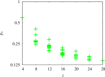
(a)

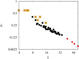
(b)

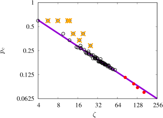
(c)

Figure 3: 3(a) Degeneracy of $p_{c}(z)$ for a square lattice with complex neighborhoods ranging from sq-1 up to sq-1,2,3,4,5,6. 3(b) Dependence $p_{c}(\xi)$ for various neighborhoods containing sites up to the sixth coordination zone. Orange crosses show equivalent neighborhoods (sq-1$\equiv$sq-2$\equiv$sq-3$\equiv$sq-5$\equiv$sq-6, sq-1,3$\equiv$sq-2,5, sq-1,2$\equiv$sq-2,3$\equiv$sq-3,5 and sq-1,2,3$\equiv$sq-2,3,5). 3(c) Dependence $p_{c}(\zeta)$. Inflated neighborhoods corresponding to higher indexes (i.e., sq-2, sq-3, sq-5, sq-6, sq-2,5, sq-2,3, sq-3,5 and sq-2,3,5) are excluded from the fitting procedure. The solid (violet) line indicates Equation 8 with $\gamma_{2}(\textsc{sq})=0.5454(60)$

In Figure 3 the dependencies of $p_{c}$ on the total number $z=\sum_{i}z_{i}$ of sites in the complex neighborhoods containing the sites of the $i$-th coordination zone and the indexes $\xi$ and $\zeta$ are presented. Figure 3(a) shows the dependence of the percolation threshold $p_{c}$ on $z$. The percolation thresholds for neighborhoods containing sites up to the fifth coordination zone are taken from References Malarz and Galam, 2005; Majewski and Malarz, 2007 and those for neighborhoods containing sites from the sixth coordination zone presented here in Table 1. It is clear that $z$ cannot differentiate between the various shapes of the neighborhoods or the percolation thresholds associated with them.

In Figure 3(b) the dependence (6) on the percolation threshold $p_{c}$ for complex neighborhoods on the square lattice on the index $\xi$ is presented. Similarly to the earlier observation for the honeycomb lattice Malarz (2022), some deviations from the straight line in Equation 6 are observed. The full circles mark percolation thresholds for compact neighbourhoods sq-1,2,$\cdots$,6,7, sq-1,2,$\cdots$,7,8, sq-1,2,$\cdots$,8,9 and sq-1,2,$\cdots$,9,10) taken from References Xun et al., 2021 and d’Iribarne et al., 1999.

Figure 3(c) shows the dependence (8) of $p_{c}$ for complex neighborhoods on the square lattice on the index $\zeta$. The percolation thresholds for neighborhoods containing sites up to the fifth coordination zone are taken from References Malarz and Galam, 2005; Majewski and Malarz, 2007, those for neighborhoods containing sites from the sixth coordination zone presented here in Table 1 and those for compact neighborhoods containing sites from the seventh to the tenth coordination zones are taken from References Xun et al., 2021 and d’Iribarne et al., 1999.

IV Discussion

The percolation thresholds $p_{c}$ obtained in simulations range from 0.59275 (for sq-6) to 0.14325 (for sq-1,2,3,4,5,6). The latter agrees in five significant digits with its earlier estimate $p_{c}(\textsc{sq-1,2,3,4,5,6})=0.143255$ Xun et al. (2021). The sq-6 neighborhood is topologically equivalent to sq-1 (but for a three-times larger lattice constant), resulting in identical percolation thresholds $p_{c}(\textsc{sq-6})=p_{c}(\textsc{sq-1})$. For the sq-6 neighborhood we deal with several simultaneous independent percolation problems on several identically shaped lattices. The latter reduces effective system size, but our results show, that this effect is perfectly compensated by effective increase of number of samples.

Similarly to the honeycomb lattice Malarz (2022), the power law (8) also holds for a square lattice with complex neighborhoods with $\gamma_{2}(\textsc{sq})=0.5454(60)$ given by the least-squares method. Inflated neighborhoods sq-2, sq-3, sq-5, sq-6, sq-2,3, sq-3,5, sq-2,5 and sq-2,3,5 (corresponding to sq-1, sq-1, sq-1, sq-1, sq-1,2, sq-1,2, sq-1,3 and sq-1,2,3, respectively) were excluded from the fitting procedure.

Among the neighborhoods that contain sites up to the sixth coordination zone, there are seven pairs of various neighborhoods with exactly the same $\zeta$ index, namely $\zeta(\textsc{sq-2,4,5,6})=\zeta(\textsc{sq-1,2,3,4,5})\approx 46.86$, $\zeta(\textsc{sq-4,5,6})=\zeta(\textsc{sq-1,3,4,5})\approx 41.20$, $\zeta(\textsc{sq-2,5,6})=\zeta(\textsc{sq-1,2,3,5})\approx 28.97$, $\zeta(\textsc{sq-2,4,6})=\zeta(\textsc{sq-1,2,3,4})\approx 35.55$, $\zeta(\textsc{sq-5,6})=\zeta(\textsc{sq-1,3,5})\approx 23.31$, $\zeta(\textsc{sq-2,6})=\zeta(\textsc{sq-1,2,3})\approx 17.66$ and $\zeta(\textsc{sq-6})=\zeta(\textsc{sq-1,3})=12$.

The differentiate power of a scalar index $\zeta$ is still better than the differentiate power of an index $\xi$ and both are much better than the differentiate power of the total number of sites in the neighborhood $z$.

V Conclusion

In this paper with Newman and Ziff effective Monte Carlo algorithm we calculated percolation thresholds for 32 complex neighbourhoods (containing sites from the sixth coordination zone) on a square lattice.

As scalar indexes $\xi$ (5) and $\zeta$ (7) allow simultaneously to (more or less effective) distinguish between various neighbourhoods and accordingly fitting $p_{c}$ to the inverse power-law on $\xi$ (6) or $\zeta$ (8) (with various efficiency depending on the underlying lattice shape) searching for another index remains an open task. The index may involve various powers of $z_{i}$, $r_{i}$ and $i$, where $i$ stands for the number of coordination zone from which sites constituting neighbourhood come from and $z_{i}$ and $r_{i}$ are the number and the distance of sites in this coordination zone to the central site in the neighbourhood, respectively.

Also calculating $p_{c}$ for neighbourhoods containing sites up to the sixth coordination zone on triangular and honeycomb lattices seems to be desired. Simultaneous calculation of $p_{c}$ for honeycomb and triangular lattices should allow for identifying inflated and equivalent neighbourhoods but among these two underlying regular lattices. Preliminary inspection of the $p_{c}(\zeta)$ dependence—but for neighbourhoods containing sites up to the fifth coordination zone Malarz (2021)—reveals $\gamma_{2}$ close to 1/2. This does not make factor $\xi$ totally useless, as for the bond-percolation problem very clear dependnce (6) with $\gamma_{1}\approx 1$ was recently observed Xun and Hao (2022).

Finally, the further studies may focus on the fractal nature of the giant component at $p=p_{c}$ Cruz et al. (2023). The largest percolating cluster on square lattice at $p=p_{c}$ has fractal properties for sq-1 neighbourhoods with fractal dimension close to 1.9 (Stauffer and Aharony, 1994, p. 9). Does this picture survive changing neighbourhoods to complex one, also on other lattice topologies? And if yes, is the fractal dimension the same as for the nearest-neighbours interactions?

The results obtained in this paper may be helpful in further searching for the universal formula, in the spirit of Equation 4 Galam and Mauger (1994), for percolation threshold $p_{c}$, also for complex neighborhoods, but independently of the underlying two-dimensional lattice shape. Also further studies on the topic presented here may result in finding universal formula for $p_{c}$ not only for two-dimensional lattices but in higher dimensions (including nonphysical dimensions, like on four- Kotwica et al. (2019); Zhao et al. (2022) and five-dimensional simple hyper-cubic Mertens and Moore (2018); Xun et al. (2023) lattices).

Appendix A Neighborhoods shapes

In Figure 4 the shapes of all complex neighborhoods containing sites from the sixth coordination zone are presented.

(a)

(b)

(c)

(d)

(e)

(f)

(g)

(h)

(i)

(j)

(k)

(l)

(m)

(n)

(o)

(p)

(q)

(r)

(s)

(t)

(u)

(v)

(w)

(x)

(y)

(z)

(aa)

(ab)

(ac)

(ad)

(ae)

Figure 4: Shapes of neighborhoods on square lattice combined with basics neighborhoods presented in Figure 1 and containing sites from the sixth coordination zone (Figure 1(f)). 4(a) sq-1,6, 4(b) sq-2,6, 4(c) sq-3,6, 4(d) sq-4,6, 4(e) sq-5,6, 4(f) sq-1,2,6, 4(g) sq-1,3,6, 4(h) sq-1,4,6, 4(i) sq-1,5,6, 4(j) sq-2,3,6, 4(k) sq-2,4,6, 4(l) sq-2,5,6, 4(m) sq-3,4,6, 4(n) sq-3,5,6, 4(o) sq-4,5,6, 4(p) sq-1,2,3,6, 4(q) sq-1,2,4,6, 4(r) sq-1,2,5,6, 4(s) sq-1,3,4,6, 4(t) sq-1,3,5,6, 4(u) sq-1,4,5,6, 4(v) sq-2,3,4,6, 4(w) sq-2,3,5,6, 4(x) sq-2,4,5,6, 4(y) sq-3,4,5,6, 4(z) sq-1,2,3,4,6, 4(aa) sq-1,2,3,5,6, 4(ab) sq-1,2,4,5,6, 4(ac) sq-1,3,4,5,6, 4(ad) sq-2,3,4,5,6, 4(ae) sq-1,2,3,4,5,6

Supplemental Material

Appendix B Boundaries procedures

Below, we present a set of boundaries() functions (written in C) to be replaced in the Newman–Ziff program published in Reference Newman and Ziff, 2001 to obtain the single realization of $\mathcal{S}_{\max}(n;L)$ for the neighborhoods presented in Figures 1(a), 1(b), 1(c), 1(d), 1(e) and 1(f).

B.1 SQ-1

boundaries() function for the sq-1 neighborhood (originally presented in Reference Newman and Ziff, 2001).

⬇

1void boundaries()

2{

3 int i,j;

4 for (i=0; i<N; i++) {

5// 1nn core:

6 nn[i][0] = (N+i +1)%N;

7 nn[i][1] = (N+i -1)%N;

8 nn[i][2] = (N+i +L)%N;

9 nn[i][3] = (N+i -L)%N;

10// 1nn left border:

11 if (i%L==0) nn[i][1] = (N+i+L -1)%N;

12// 1nn right border:

13 if ((i+1)%L==0) nn[i][0] = (N+i-L +1)%N;

14 }

15}

B.2 SQ-2

boundaries() function for the sq-2 neighborhood.

⬇

1void boundaries()

2{

3 int i,j;

4 for (i=0; i<N; i++) {

5// 2nn core:

6 nn[i][0] = (N+i +L+1)%N;

7 nn[i][1] = (N+i +L-1)%N;

8 nn[i][2] = (N+i -L+1)%N;

9 nn[i][3] = (N+i -L-1)%N;

10// 2nn left border:

11 if(i%L==0) {

12 nn[i][1] = (N+i+L +L-1)%N;

13 nn[i][3] = (N+i+L -L-1)%N; }

14// 2nn right border:

15 if((i+1)%L==0) {

16 nn[i][0] = (N+i-L +L+1)%N;

17 nn[i][2] = (N+i-L -L+1)%N; }

18 }

19}

B.3 SQ-3

boundaries() function for the sq-3 neighborhood.

⬇

1void boundaries()

2{

3 int i,j;

4 for (i=0; i<N; i++) {

5// 3nn core:

6 nn[i][0] = (N+i +2*L)%N;

7 nn[i][1] = (N+i -2*L)%N;

8 nn[i][2] = (N+i +2)%N;

9 nn[i][3] = (N+i -2)%N;

10// 3nn left border:

11 if(i%L==0 || i%L==1)

12 nn[i][3] = (N+i+L -2)%N;

13// 3nn right border:

14 if((i+1)%L==0 || (i+2)%L==0)

15 nn[i][2] = (N+i-L +2)%N;

16 }

17}

B.4 SQ-4

boundaries() function for the neighborhood sq-4. The preprocesor directive #define Z 4 in source code in Reference Newman and Ziff, 2001 requires replacing to #define Z 8.

⬇

1void boundaries()

2{

3 int i,j;

4 for (i=0; i<N; i++) {

5// 4nn core:

6 nn[i][0] = (N+i +L+2)%N;

7 nn[i][1] = (N+i +L-2)%N;

8 nn[i][2] = (N+i -L+2)%N;

9 nn[i][3] = (N+i -L-2)%N;

10 nn[i][4] = (N+i +2*L+1)%N;

11 nn[i][5] = (N+i +2*L-1)%N;

12 nn[i][6] = (N+i -2*L+1)%N;

13 nn[i][7] = (N+i -2*L-1)%N;

14// 4nn left border:

15 if(i%L==0 || i%L==1 ) {

16 nn[i][1] = (N+i+L +L-2)%N;

17 nn[i][3] = (N+i+L -L-2)%N;

18 nn[i][5] = (N+i+L +2*L-1)%N;

19 nn[i][7] = (N+i+L -2*L-1)%N; }

20// 4nn right border:

21 if((i+1)%L==0 || (i+2)%L==0) {

22 nn[i][0] = (N+i-L +L+2)%N;

23 nn[i][2] = (N+i-L -L+2)%N;

24 nn[i][4] = (N+i-L +2*L+1)%N;

25 nn[i][6] = (N+i-L -2*L+1)%N; }

26 }

27}

B.5 SQ-5

boundaries() function for the sq-5 neighborhood.

⬇

1void boundaries()

2{

3 int i,j;

4 for (i=0; i<N; i++) {

5// 5nn core:

6 nn[i][0] = (N+i +2*L+2)%N;

7 nn[i][1] = (N+i +2*L-2)%N;

8 nn[i][2] = (N+i -2*L+2)%N;

9 nn[i][3] = (N+i -2*L-2)%N;

10// 5nn left border:

11 if(i%L==0 || i%L==1) {

12 nn[i][1] = (N+i+L +2*L-2)%N;

13 nn[i][3] = (N+i+L -2*L-2)%N; }

14// 5nn right border:

15 if((i+1)%L==0 || (i+2)%L==0) {

16 nn[i][0] = (N+i-L +2*L+2)%N;

17 nn[i][2] = (N+i-L -2*L+2)%N; }

18 }

19}

B.6 SQ-6

boundaries() function for the sq-6 neighborhood.

⬇

1void boundaries()

2{

3 int i,j;

4 for (i=0; i<N; i++) {

5// 6nn core:

6 nn[i][0] = (N+i +3*L)%N;

7 nn[i][1] = (N+i -3*L)%N;

8 nn[i][2] = (N+i +3)%N;

9 nn[i][3] = (N+i -3)%N;

10// 6nn left border:

11 if(i%L==0 || i%L==1 || i%L==2)

12 nn[i][3] = (N+i+L -3)%N;

13// 6nn right border:

14 if((i+1)%L==0 || (i+2)%L==0 || (i+3)%L==0)

15 nn[i][2] = (N+i-L +3)%N;

16 }

17}

Appendix C Dependencies of $\mathcal{P}_{\max}\cdot L^{\beta/\nu}$ on the probability of occupation $p$

Figure 7 presents the dependencies of $\mathcal{P}_{\max}\cdot L^{\beta/\nu}$ on the probability of occupation $p$ for neighborhoods ranging from sq-6 to sq-1,2,3,4,5,6 for various linear system sizes $L=128$, 256, 512, 1024, 2048, and 4096.

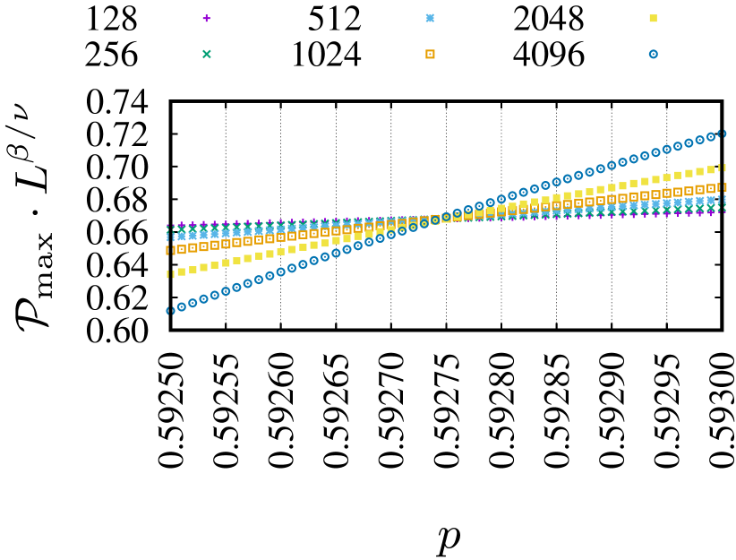
(a)

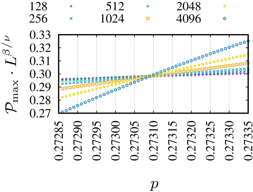
(b)

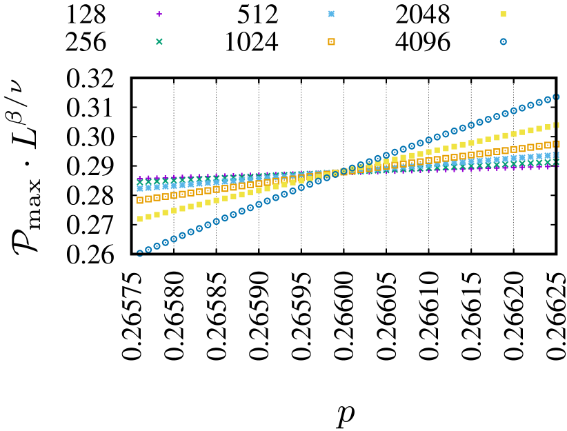
(c)

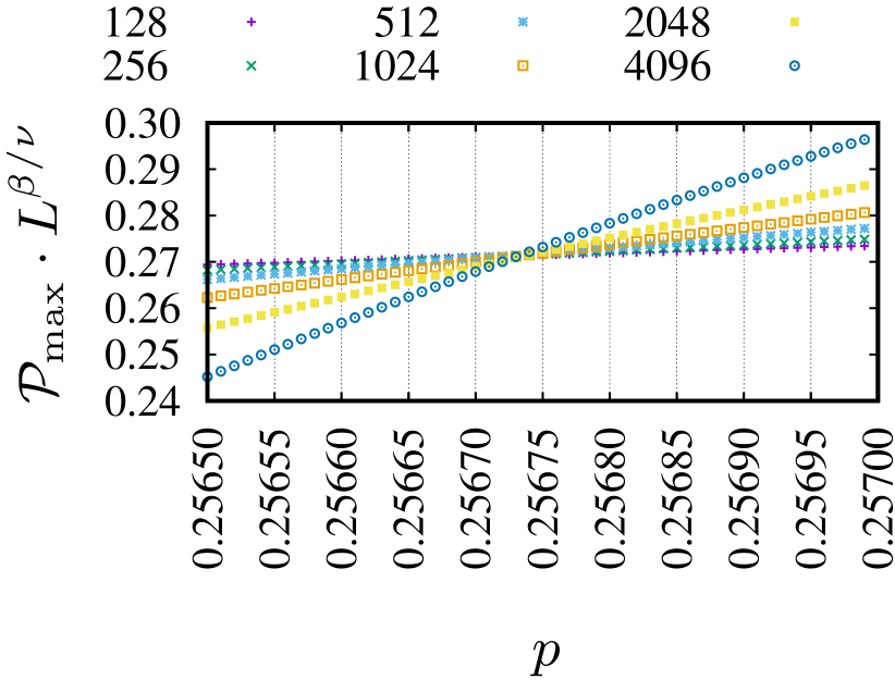
(d)

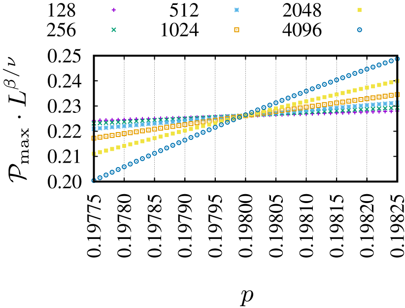
(e)

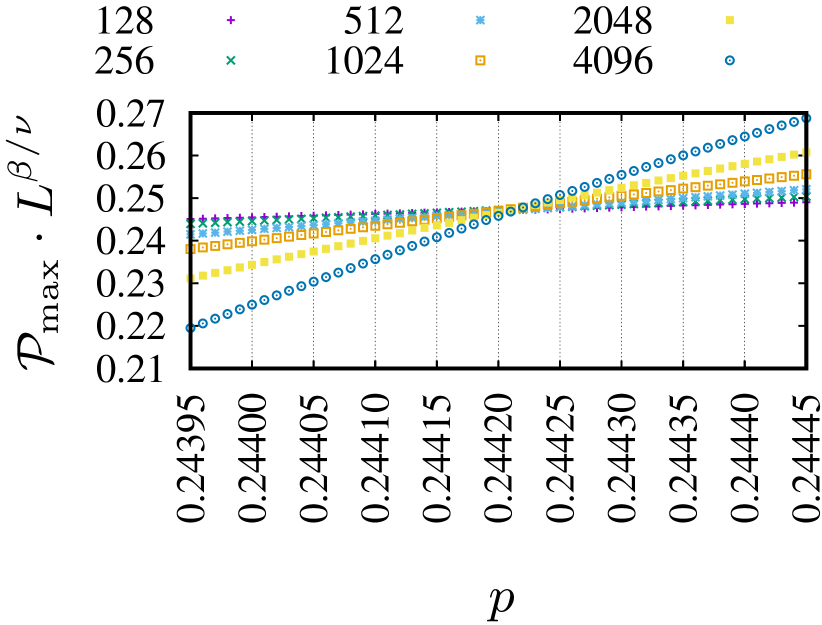
(f)

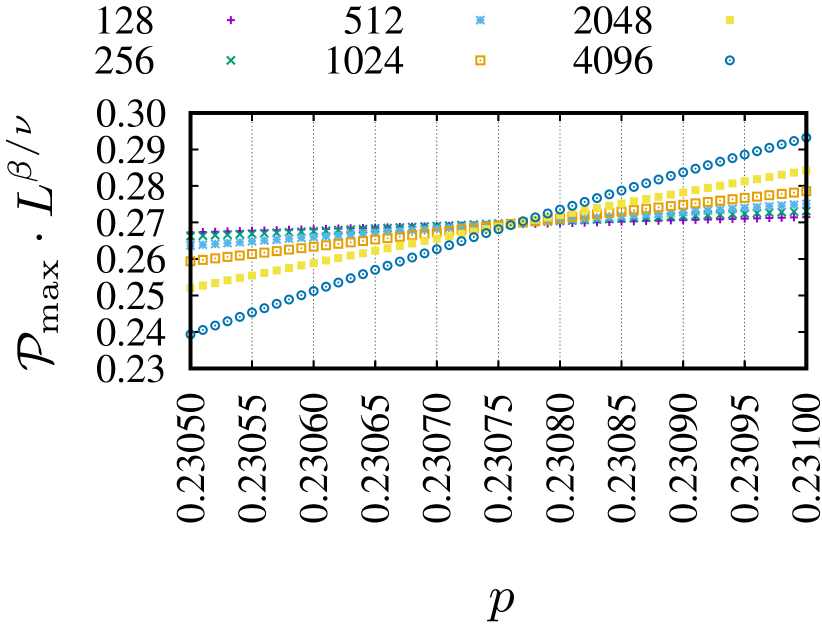
(g)

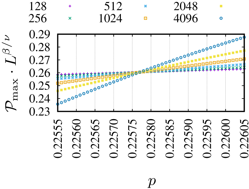
(h)

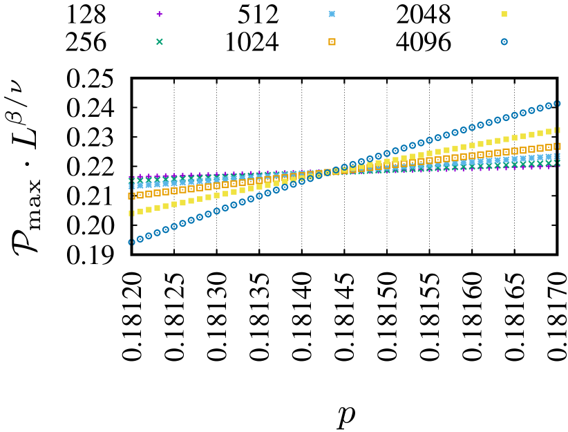
(i)

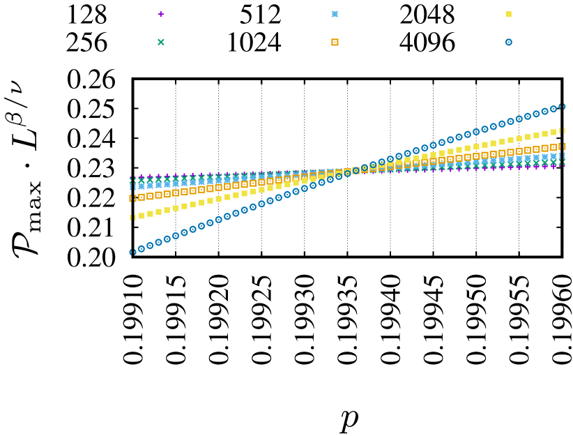
(j)

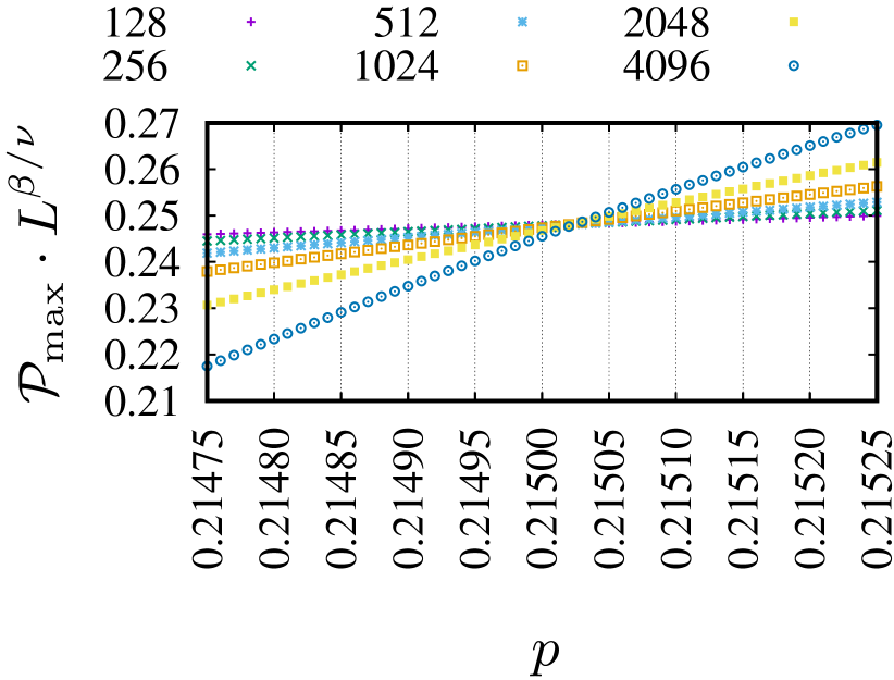
(k)

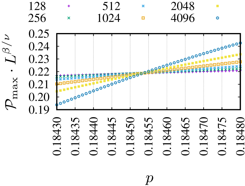
(l)

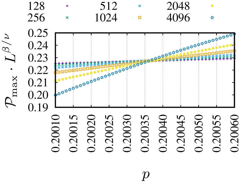
(m)

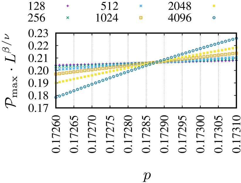
(n)

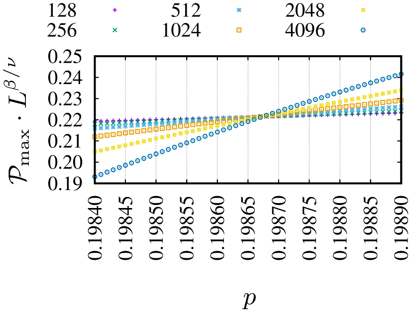
(o)

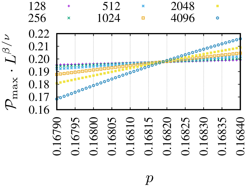
(a)

(b)

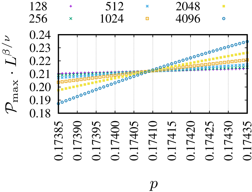
(c)

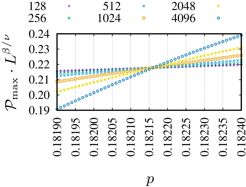
(d)

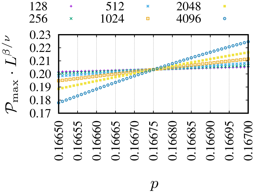
(e)

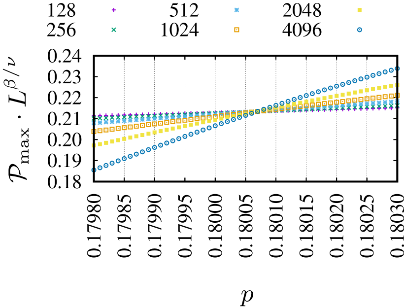
(f)

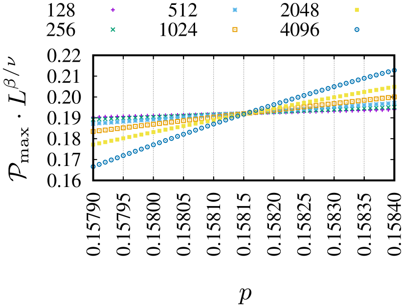
(g)

(h)

(i)

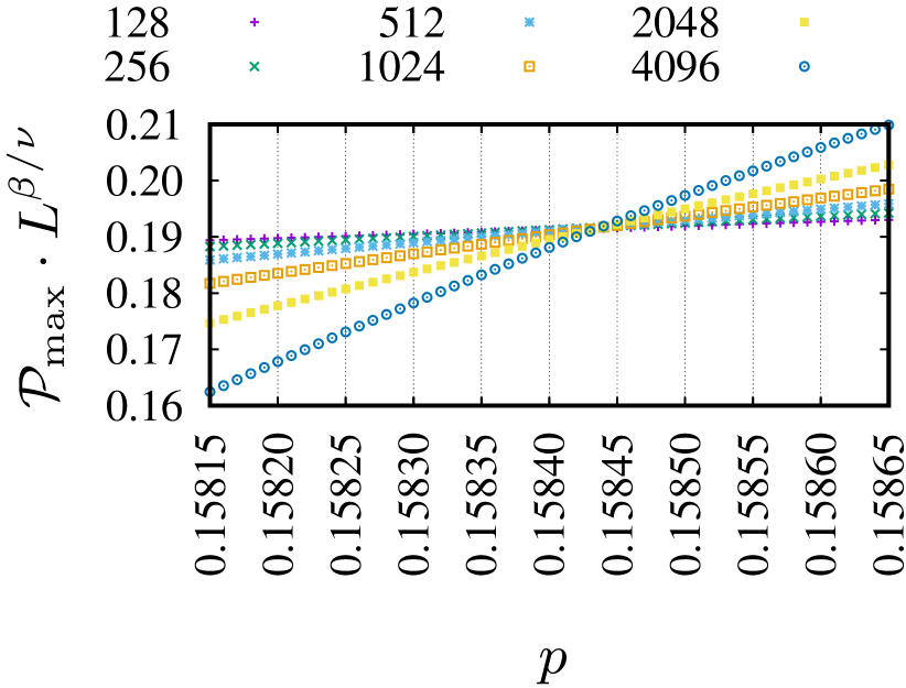
(j)

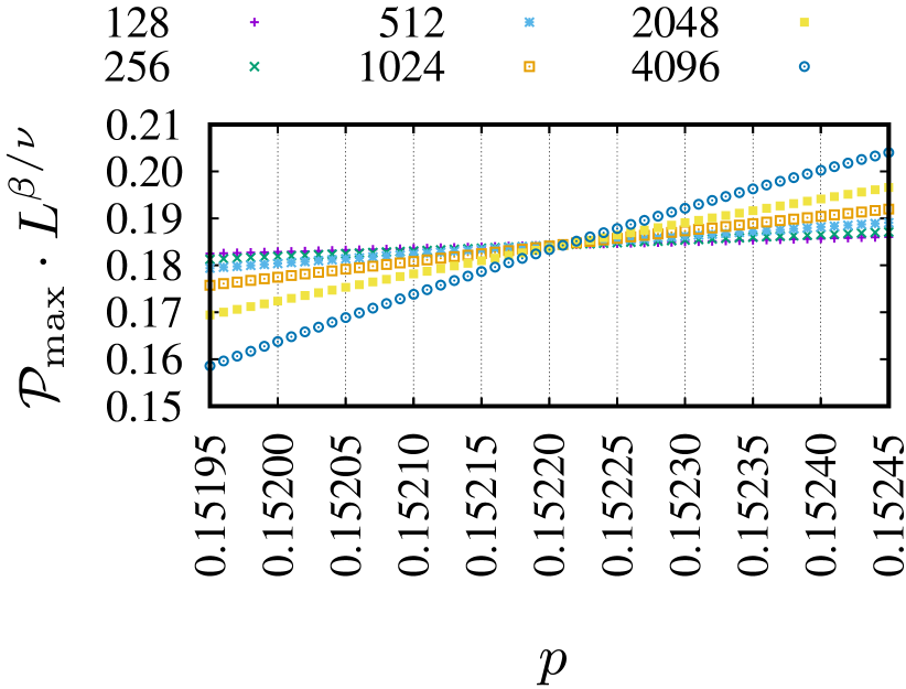
(k)

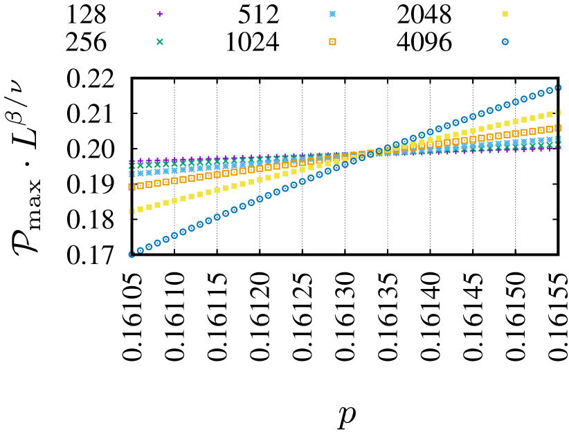
(l)

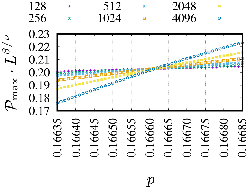
(m)

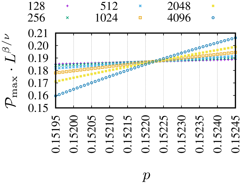
(n)

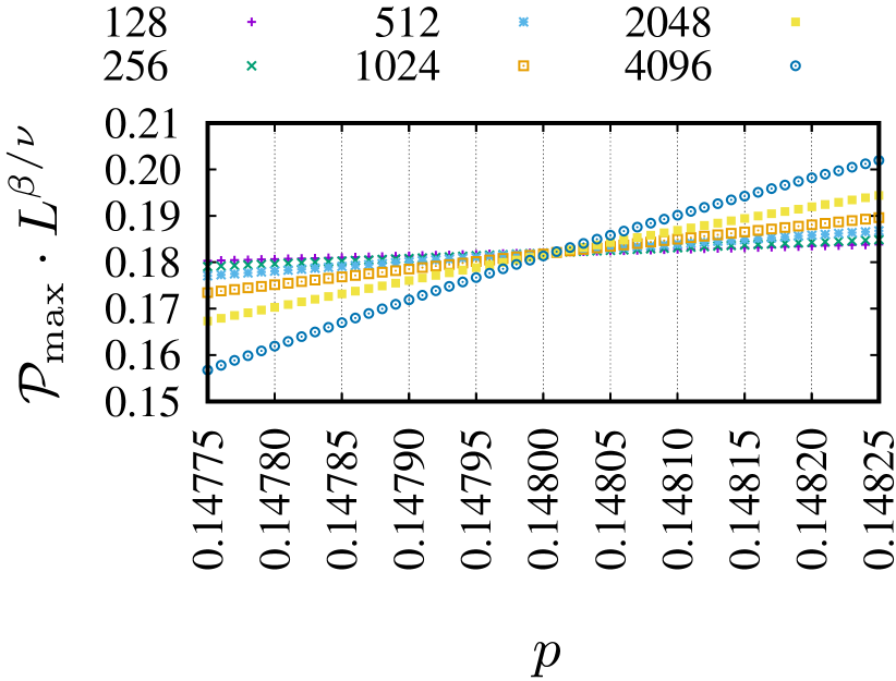
(o)

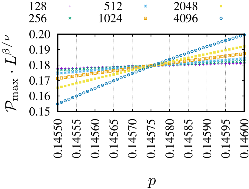
(a)

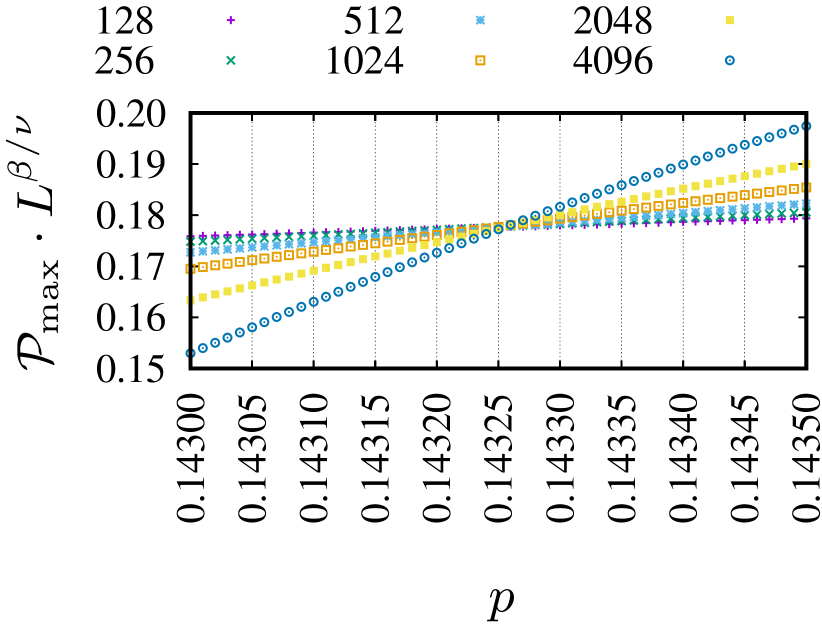
(b)

Figure 7: $L^{\varepsilon_{1}}\mathcal{P}_{\text{max}}$ vs. $p$ for various complex neighborhoods and various values of $L$ indicated in the title of the figures. The results are averaged over the realizations of the $R=10^{5}$ system. The probability of occupation $p$ is scanned with $\Delta p=10^{-5}$ separation step. 5(a) sq-6, 5(b) sq-1,6, 5(c) sq-2,6, 5(d) sq-3,6, 5(e) sq-4,6, 5(f) sq-5,6, 5(g) sq-1,2,6, 5(h) sq-1,3,6, 5(i) sq-1,4,6, 5(j) sq-1,5,6, 5(k) sq-2,3,6, 5(l) sq-2,4,6, 5(m) sq-2,5,6, 5(n) sq-3,4,6, 5(o) sq-3,5,6, 6(a) sq-4,5,6, 6(b) sq-1,2,3,6, 6(c) sq-1,2,4,6, 6(d) sq-1,2,5,6, 6(e) sq-1,3,4,6, 6(f) sq-1,3,5,6, 6(g) sq-1,4,5,6, 6(h) sq-2,3,4,6, 6(i) sq-2,3,5,6, 6(j) sq-2,4,5,6, 6(k) sq-3,4,5,6, 6(l) sq-1,2,3,4,6, 6(m) sq-1,2,3,5,6, 6(n) sq-1,2,4,5,6, 6(o) sq-1,3,4,5,6, 7(a) sq-2,3,4,5,6, 7(b) sq-1,2,3,4,5,6

References

- Broadbent and Hammersley (1957) S. R. Broadbent and J. M. Hammersley, “Percolation processes: I. Crystals and mazes,” Mathematical Proceedings of the Cambridge Philosophical Society 53, 629–641 (1957).
- Hammersley (1957) J. M. Hammersley, “Percolation processes: II. The connective constant,” Mathematical Proceedings of the Cambridge Philosophical Society 53, 642–645 (1957).
- Cheng et al. (2020) L. Cheng, P. Yan, X. Yang, H. Zou, H. Yang, and H. Liang, “High conductivity, percolation behavior and dielectric relaxation of hybrid ZIF-8/CNT composites,” Journal of Alloys and Compounds 825, 154132 (2020).
- Zhang et al. (2020) Q. Zhang, B.-Y. Zhang, B.-H. Guo, Z.-X. Guo, and J. Yu, “High-temperature polymer conductors with self-assembled conductive pathways,” Composites Part B—Engineering 192, 107989 (2020).
- Malarz et al. (2002) K. Malarz, S. Kaczanowska, and K. Kułakowski, “Are forest fires predictable?” International Journal of Modern Physics C 13, 1017–1031 (2002).
- Ramírez et al. (2020) J. E. Ramírez, C. Pajares, M. I. Martínez, R. Rodríguez Fernández, E. Molina-Gayosso, J. Lozada-Lechuga, and A. Fernández Téllez, “Site-bond percolation solution to preventing the propagation of Phytophthora zoospores on plantations,” Physical Review E 101, 032301 (2020).
- Ghanbarian et al. (2020) B. Ghanbarian, F. Liang, and H.-H. Liu, “Modeling gas relative permeability in shales and tight porous rocks,” Fuel 272, 117686 (2020).
- Ziff (2021) R. M. Ziff, “Percolation and the pandemic,” Physica A: Statistical Mechanics and its Applications 568, 125723 (2021).
- Dong et al. (2020) S. Dong, A. Mostafizi, H. Wang, J. Gao, and X. Li, “Measuring the topological robustness of transportation networks to disaster-induced failures: A percolation approach,” Journal of Infrastructure Systems 26, 04020009 (2020).
- Cao et al. (2020) W. Cao, L. Dong, L. Wu, and Y. Liu, “Quantifying urban areas with multi-source data based on percolation theory,” Remote Sensing of Environment 241, 111730 (2020).
- Bartolucci et al. (2020) S. Bartolucci, F. Caccioli, and P. Vivo, “A percolation model for the emergence of the Bitcoin Lightning Network,” Scientific Reports 10, 4488 (2020).
- Li et al. (2021) M. Li, R.-R. Liu, L. Lü, M.-B. Hu, S. Xu, and Y.-C. Zhang, “Percolation on complex networks: Theory and application,” Physics Reports 907, 1–68 (2021).
- Saberi (2015) A. A. Saberi, “Recent advances in percolation theory and its applications,” Physics Reports 578, 1–32 (2015).
- Stauffer and Aharony (1994) D. Stauffer and A. Aharony, Introduction to Percolation Theory, 2nd ed. (Taylor and Francis, London, 1994).
- Wierman (2014) J. Wierman, “Percolation theory,” in Wiley StatsRef: Statistics Reference Online (American Cancer Society, 2014) pp. 1–9.
- Dean (1963) P. Dean, “A new Monte Carlo method for percolation problems on a lattice,” Mathematical Proceedings of the Cambridge Philosophical Society 59, 397–410 (1963).
- Dean and Bird (1967) P. Dean and N. F. Bird, “Monte Carlo estimates of critical percolation probabilities,” Mathematical Proceedings of the Cambridge Philosophical Society 63, 477–479 (1967).
- Suding and Ziff (1999) P. N. Suding and R. M. Ziff, “Site percolation thresholds for Archimedean lattices,” Physical Review E 60, 275–283 (1999).
- Dalton et al. (1964) N. W. Dalton, C. Domb, and M. F. Sykes, “Dependence of critical concentration of a dilute ferromagnet on the range of interaction,” Proceedings of the Physical Society 83, 496–498 (1964).
- Domb and Dalton (1966) C. Domb and N. W. Dalton, “Crystal statistics with long-range forces: I. The equivalent neighbour model,” Proceedings of the Physical Society 89, 859–871 (1966).
- Gouker and Family (1983) M. Gouker and F. Family, “Evidence for classical critical behavior in long-range site percolation,” Physical Review B 28, 1449–1452 (1983).
- Malarz and Galam (2005) K. Malarz and S. Galam, “Square-lattice site percolation at increasing ranges of neighbor bonds,” Physical Review E 71, 016125 (2005).
- Galam and Malarz (2005) S. Galam and K. Malarz, “Restoring site percolation on damaged square lattices,” Physical Review E 72, 027103 (2005).
- Majewski and Malarz (2007) M. Majewski and K. Malarz, “Square lattice site percolation thresholds for complex neighbourhoods,” Acta Physica Polonica B 38, 2191–2199 (2007).
- Xun et al. (2021) Z. Xun, D. Hao, and R. M. Ziff, “Site percolation on square and simple cubic lattices with extended neighborhoods and their continuum limit,” Physical Review E 103, 022126 (2021).
- d’Iribarne et al. (1999) C. d’Iribarne, M. Rasigni, and G. Rasigni, “From lattice long-range percolation to the continuum one,” Physics Letters A 263, 65–69 (1999).
- Malarz (2020) K. Malarz, “Site percolation thresholds on triangular lattice with complex neighborhoods,” Chaos 30, 123123 (2020).
- Malarz (2021) K. Malarz, “Percolation thresholds on triangular lattice for neighbourhoods containing sites up-to the fifth coordination zone,” Physical Review E 103, 052107 (2021).
- Malarz (2022) K. Malarz, “Random site percolation on honeycomb lattices with complex neighborhoods,” Chaos 32, 083123 (2022).
- Lebrecht et al. (2021) W. Lebrecht, P. M. Centres, and A. J. Ramirez-Pastor, “Empirical formula for site and bond percolation thresholds on Archimedean and 2-uniform lattices,” Physica A: Statistical Mechanics and its Applications 569, 125802 (2021).
- Xun et al. (2022) Z. Xun, D. Hao, and R. M. Ziff, “Site and bond percolation thresholds on regular lattices with compact extended-range neighborhoods in two and three dimensions,” Physical Review E 105, 024105 (2022).
- Kurzawski and Malarz (2012) Ł. Kurzawski and K. Malarz, “Simple cubic random-site percolation thresholds for complex neighbourhoods,” Reports on Mathematical Physics 70, 163–169 (2012).
- Malarz (2015) K. Malarz, “Simple cubic random-site percolation thresholds for neighborhoods containing fourth-nearest neighbors,” Physical Review E 91, 043301 (2015).
- Kotwica et al. (2019) M. Kotwica, P. Gronek, and K. Malarz, “Efficient space virtualisation for Hoshen–Kopelman algorithm,” International Journal of Modern Physics C 30, 1950055 (2019).
- Zhao et al. (2022) P. Zhao, J. Yan, Z. Xun, D. Hao, and R. M. Ziff, “Site and bond percolation on four-dimensional simple hypercubic lattices with extended neighborhoods,” Journal of Statistical Mechanics: Theory and Experiment 2022, 033202 (2022).
- Xu et al. (2021) W. Xu, J. Wang, H. Hu, and Y. Deng, “Critical polynomials in the nonplanar and continuum percolation models,” Physical Review E 103, 022127 (2021).
- Koza et al. (2014) Z. Koza, G. Kondrat, and K. Suszczyński, “Percolation of overlapping squares or cubes on a lattice,” Journal of Statistical Mechanics: Theory and Experiment 2014, P11005 (2014).
- Koza and Poła (2016) Z. Koza and J. Poła, “From discrete to continuous percolation in dimensions 3 to 7,” Journal of Statistical Mechanics: Theory and Experiment 2016, 103206 (2016).
- Galam and Mauger (1996) S. Galam and A. Mauger, “Universal formulas for percolation thresholds,” Physical Review E 53, 2177–2181 (1996).
- Galam and Mauger (1997) S. Galam and A. Mauger, “Reply to “Comment on ‘Universal formulas for percolation thresholds”’,” Physical Review E 55, 1230–1231 (1997).
- van der Marck (1997) S. C. van der Marck, “Universal formulas for percolation thresholds — Comment,” Physical Review E 55, 1228–1229 (1997).
- Newman and Ziff (2001) M. E. J. Newman and R. M. Ziff, “Fast Monte Carlo algorithm for site or bond percolation,” Physical Review E 64, 016706 (2001).
- Privman (1990) V. Privman, “Finite-size scaling theory,” in Finite size scaling and numerical simulation of statistical systems, edited by V. Privman (World Scientific, Singapore, 1990) pp. 1–98.
- Landau and Binder (2009) D. P. Landau and K. Binder, A Guide to Monte Carlo Simulations in Statistical Physics, 3rd ed. (Cambridge University Press, 2009).
- Newman and Ziff (2000) M. E. J. Newman and R. M. Ziff, “Efficient Monte Carlo algorithm and high-precision results for percolation,” Physical Review Letters 85, 4104–4107 (2000).
- Tencer and Forsberg (2021) J. Tencer and K. M. Forsberg, “Postprocessing techniques for gradient percolation predictions on the square lattice,” Physical Review E 103, 012115 (2021).
- Xun and Hao (2022) Z. Xun and D. Hao, “Monte Carlo simulation of bond percolation on square lattice with complex neighborhoods,” Acta Physica Sinica 71, 066401 (2022), in Chinese.
- Cruz et al. (2023) M.-Á. M. Cruz, J. P. Ortiz, M. P. Ortiz, and A. Balankin, “Percolation on fractal networks: A survey,” Fractal and Fractional 7, 231 (2023).
- Galam and Mauger (1994) S. Galam and A. Mauger, “A new scheme to percolation thresholds,” J. Appl. Phys. 75, 5526–5528 (1994).
- Mertens and Moore (2018) S. Mertens and C. Moore, “Percolation thresholds and Fisher exponents in hypercubic lattices,” Physical Review E 98, 022120 (2018).
- Xun et al. (2023) Z. Xun, D. Hao, and R. M. Ziff, “Extended-range percolation in five dimensions,” (2023), arXiv:2308.15719 [cond-mat.stat-mech] .