Identification of Novel Classes for Improving Few-Shot Object Detection

Abstract

Conventional training of deep neural networks requires a large number of the annotated image which is a laborious and time-consuming task, particularly for rare objects. Few-shot object detection (FSOD) methods offer a remedy by realizing robust object detection using only a few training samples per class. An unexplored challenge for FSOD is that instances from unlabeled novel classes that do not belong to the fixed set of training classes appear in the background. These objects behave similarly to label noise, leading to FSOD performance degradation. We develop a semi-supervised algorithm to detect and then utilize these unlabeled novel objects as positive samples during training to improve FSOD performance. Specifically, we propose a hierarchical ternary classification region proposal network (HTRPN) to localize the potential unlabeled novel objects and assign them new objectness labels. Our improved hierarchical sampling strategy for the region proposal network (RPN) also boosts the perception ability of the object detection model for large objects. Our experimental results indicate that our method is effective and outperforms the existing state-of-the-art (SOTA) FSOD methods. https://github.com/zshanggu/HTRPN

1 Introduction

The adoption of deep neural network architectures in object detection has led to a significant method in determining the location and the category of objects of interest in an image. In the presence of abundant training data, object detection models based on the region-based convolution neural networks (R-CNN) architecture reach high accuracy on most object detection tasks. However, preparing large-scale annotated training data can be a challenging task in some applications, e.g., miscellaneous disease analysis and industrial defect detection. In the presence of insufficient training data, these models easily overfit and fail to generalize well. In contrast, humans are able a novel object class very fast based on a few samples. As a result, it is extremely desirable to develop models that can learn object classes using only a few samples, known as few-shot object detection (FSOD).

Current FSOD methods are based on pre-training a suitable model on a set of base classes with abundant training data and then fine-tuning the model on both the base classes and the novel classes for which only a few samples are accessible (see Figure 1). The primary approach in FSOD is to benefit from ideas in transfer learning or meta-learning to learn novel classes through the knowledge obtained during the pre-training stage while maintaining good performance in base classes. Despite recent advances in FSOD, current SOTA methods are still far from getting favorable results on novel classes similar to the base classes. Potential reasons for this performance gap include the confusion between visually similar categories, incorrect annotations (label noise), the existence of unseen novel objects during training, etc. Recent FSOD methods have focused on addressing these challenges for improved FSOD performance.

Figure 1: FSOD methods pre-train a model on abundant base classes and then fine-tune it on both base and novel classes.

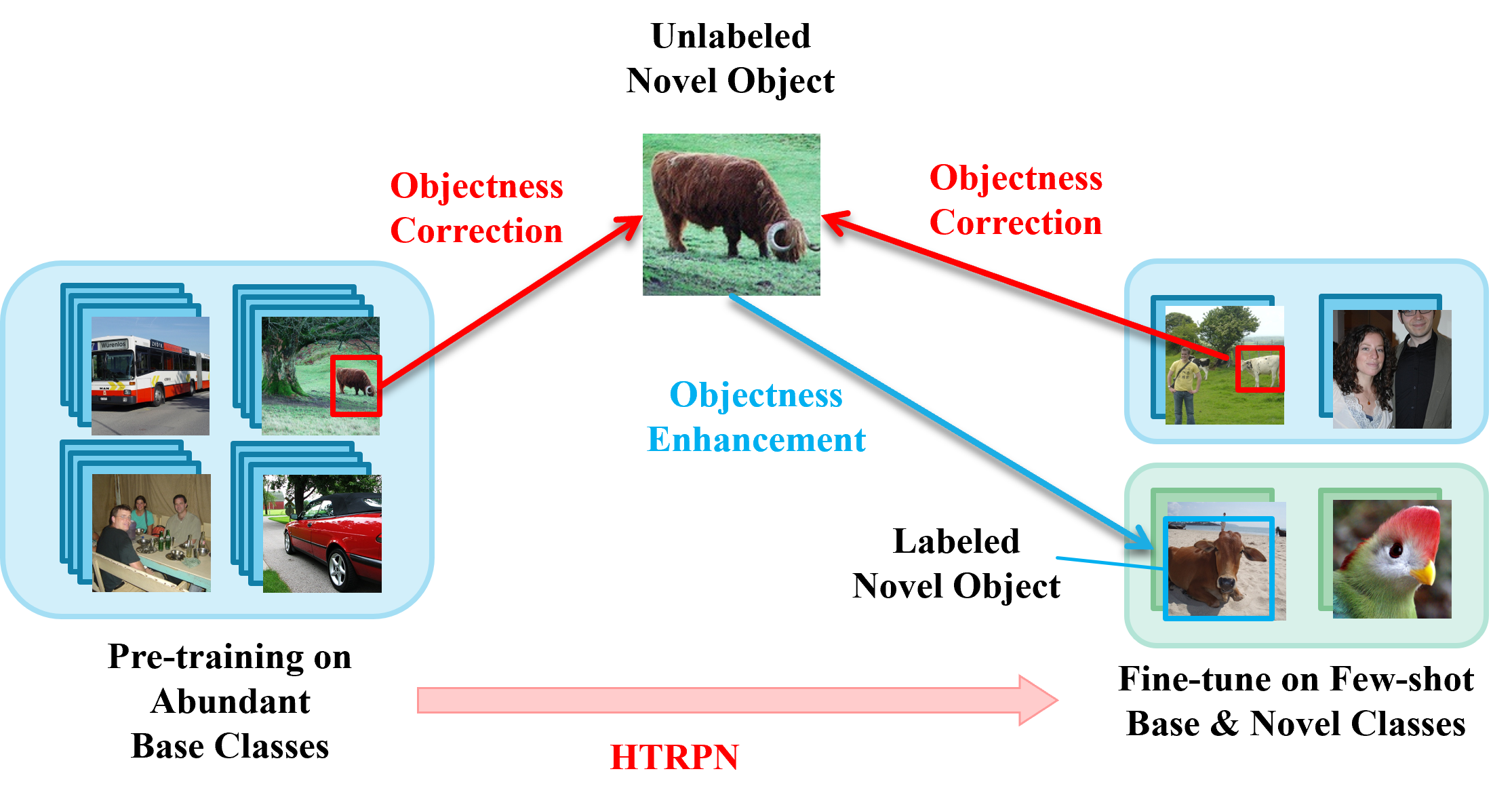
We study the phenomenon that unlabeled novel object classes that do not belong to either of the base or the labeled novel classes can appear in the training data. For example, we see in Figure. 1 that among base-class training samples, there are a number of objects that remain unlabeled, such as the cow in the image. These unlabeled objects can potentially belong to unseen novel classes. Our experiments demonstrate that this phenomenon exists in PASCAL VOC [4] and COCO [21] datasets.This phenomenon leads to the objectness inconsistency for the model when recognizing the novel objects: for the novel class, objects are treated as background if their annotations are missing, but they are treated as foreground where they are labeled. Such nonconformity of foreground and background confuses the model when training the objectness and make the model hard to converge and degrades detection accuracy.

To tackle the above challenge, we develop a semi-supervised learning method to utilize the potential novel objects that appear during training to improve the ability of the model to recognize novel classes. We first demonstrate the possibility of detecting these unlabeled objects. Our experiment indicates that some unlabeled class objects are likely to be recognized if they are similar to the training base and novel classes. We collect the unlabeled novel objects from the background proposals by determining whether they are predicted as known classes, and then we give these proposals an extra objectness label in the region proposal network (RPN) so that the model could learn them. We also analyze the defect of the standard RPN in detecting objects of different sizes during training and propose a more balanced RPN sampling method so that objects are treated equally in all scales. We provide extensive experimental results to demonstrate the effectiveness of our method on the PASCAL VOC and COCO datasets. Our contributions include:

• We modify the anchor sampling strategy so that the anchors are evenly chosen from different layers of the feature pyramid layer in the R-CNN architecture.

• We design a ternary objectness classification in the RPN layer which enables the model to recognize potential novel class objects to improve consistency.

• We use contrastive learning in the RPN layer to distinguish between the positive and the negative anchors.

2 Related works

We assume that there are three classes: base classes, seen novel classes, and unseen novel classes. The base and the seen novel classes form the training dataset. For base classes, we have sufficient data but for seen novel classes, we have a few samples per class. Most works in FSOD only consider these classes. The unseen novel classes are not included in the training data but emerge as novel classes in the background.

Few-shot object detection Typical object detection networks are usually either two-stage or one-stage. For two-stage object detection networks, such as R-CNN  [9], R-FCN  [3], Fast-RCNN  [8], and Faster-RCNN  [28], the model first applies fixed anchors in the region proposal network (RPN) to determine if a proposal box contains an object. The selected proposals then are sent to the region of interest (RoI) pooling layer to get an instance-level classification and bounding boxes. One-stage object detection networks such as SSD  [22], YOLO series  [26, 27], and Overfeat  [30], estimate the category and the location of an object directly from the backbone network without RPN. Two-stage object detection networks have higher detecting accuracy than one-stage schemes but lower inference speed  [17]. Few-shot object detection (FSOD), is a case of object detection that only a few samples are available for training.

Two-stage FSOD For FSOD, the model is usually first pre-trained on the base classes for which we have data-sufficient. The model is then, fine-tuned on the seen novel classes  [35], each with a few samples. As for the fine-tuning stage, meta-learning and transfer learning are two major end-to-end approaches. Methods based on meta-learning [5, 10, 11, 42] build an inquiry set and a support set that contains $k$ categories with $n$ samples in each, namely $k$-way $n$-shot setting. By creating the $k$-way $n$-shot episodes for training, meta-learning help to learn a metric to determine which support set category an inquiry image belongs to [5, 10, 11, 42]. In contrast, methods based on transfer learning start from the pre-training weights and fine-tune the model on the novel seen classes  [35, 31].

Unseen novel objects In an object detection problem, the set of the base and the seen novel classes are assumed to be a closed set. However, there may be potential novel unseen objects in the training data that do not belong to the initial set of classes. These objects naturally are classified as one of seen classes and hence, there has been an interest to mitigate the adverse effects of these objects. Semi-supervised object detection network is a potential solution for this problem which utilizes the challenging samples  [29, 24, 41]. Kaul et al.  [15] build a class-specific self-supervised label verification model to identify candidates of unlabeled (unseen) objects and give them pseudo-annotations. The model is then retrained with these pseudo-annotated samples to improve the object-detecting accuracy. However, this method requires two rounds of training and requires extra effort to adapt to other categories. Li et al.  [20] propose a distractor utilization loss by giving the distractor proposals a pseudo-label during fine-tuning. This method is used only in the fine-tuning stage and hence, the objectness inconsistency from the pre-training stage is not addressed. Inspired by these shortcomings, we propose utilizing the unlabeled potential objects that belong to the unseen classes to reduce the negative effect of novel objects.

Contrastive learning can be used to enlarge the inter-class distances and narrow down the intra-class distances for classification tasks to enhance data representations. It has been applied to many classification tasks in topics such as visual recognition  [25, 33], semantic segmentation  [34], super-resolution  [36], and natural language processing  [7, 2]. Self-supervised contrastive learning in few-shot object detection is introduced by FSCE [31] to better distinguish similar categories at the instance level during fine-tuning. We benefit from a similar strategy in our work.

(a)

(b)

(c)

(d)

Figure 2: The left images in each row indicate the predicted boxes with the class names and confidence, and the right images are the feature maps of the RPN layer.

3 Problem Description

We formulate the problem of FSOD following a standard setting in the literature [13, 35]. We use the Faster R-CNN network as the object detection model and follow the same evaluation paradigm defined by  [35]. Accordingly, the base classes are those classes for which we have sufficient images and instances for each base class ($C_{B}$), while novel classes are those for which, we only have a few training samples in the dataset ($C_{N}$), where $C_{B}\cap C_{N}=\varnothing$. An $n$-shot learning scenario means that we have access to $n$ images per seen novel categories. During the pre-training stage, the model is trained only on base class $C_{B}$, and also is only evaluated on the test set of $C_{B}$. We then proceed to learn the seen novel classes in the second stage. To overcome catastrophic forgetting about the learned knowledge about the base classes, the pre-trained model is then fine-tuned on both the seen novel classes and base classes $C_{N}\cup C_{B}$ and then is tested on both sets of classes.

Architectures based on R-CNN have been used consistently for object detection. In our work, we improve the R-CNN architecture to identify novel unseen classes as instances that do not belong to the seen classes. For an input image, R-CNN derives five scaled feature maps ($p2\sim p6$) using its feature pyramid network (FPN), and then size-fixed anchors in the region proposal network (RPN) are applied on these feature maps to predict the objectness (i.e., $obj\{obj_{pre},obj_{gt},iou_{gt}^{a}\}$, where $obj_{pre}$ is the predicted objectness score in the range of 0 and 1. Here, the ground truth value $obj_{gt}=0$ indicates a non-object and $obj_{gt}=1$ represents a true object, and $iou_{gt}^{a}$ represents the intersection over the union of an anchor with its ground truth box) and the coarse bounding box (i.e., $bbox_{c}$) of each anchor to get proposal boxes (i.e., $Prop\{obj,bbox_{c},iou_{gt}^{p}\}$, $iou_{gt}^{p}$ represents the intersection over the union of a proposal box with its ground truth box). Anchors with $iou_{gt}^{a}>0.7$ are called active anchors ($A_{a}$) and their corresponding proposals are called positive proposals ($Prop_{p}$); while anchors with $iou_{gt}^{a}<0.3$ are called negative anchors ($A_{n}$) and the corresponding proposals are called negative proposals ($Prop_{n}$). Next, $Prop_{p}$ and $Prop_{n}$ are sent to the region of interest pooling layer (RoI pooling) to predict their instance level classification (i.e., $cls^{i}$, where $i$ is the classification index) and the refined bounding box (i.e., $bbox_{r}$). The objects ($Obj\{cls^{i},bbox_{r}\}$) are then finally detected.

(a)

(b)

Figure 3: Novel unseen classes versus novel seen classes: (a) a schematic diagram of how coarse anchors work. For an $n\times m$ feature map, 3 fixed anchors will be applied on each pixel of it. Therefore, each feature map would have $3m\times n$ coarse anchors. (b) The mechanism of our proposed HSamp can equally choose anchors for each layer.

(a)

(b)

(c)

(d)

(e)

(f)

(g)

(h)

(i)

(j)

(k)

(l)

Figure 4: The original image and anchors of p2/p3/p4/p5/p6 layers: (a)-(f) in the original FRCN, we hardly have chance to pick up negative anchors that contain large novel unseen class objects. (g)-(l) when HSamp is used, the anchors are more balanced for each layer and the large objects are more likely to be contained.

The challenge that we want to address stems from the fact that an instance from the unlabeled and unseen novel object (${C_{N}}^{pn}$) can appear in the training dataset in the background (see Figure 2). The reason is that there are many potential classes that we have not included in either the base classes or the unseen novel classes. When detected, these objects would be treated as $Prop_{n}$ and with its ground truth objectness ${obj_{gt}}^{pn}=0$. On the contrary, they would be treated as $Prop_{p}$ with ground truth objectness ${obj_{gt}}^{pn}=1$ if it is labeled as such by the model. These instances can significantly confuse the model when adapting the model for learning the novel unseen classes. We argue that if the unlabeled potential novel object can be distinguished from the $Prop_{n}$, then its objectness could be modified as a foreground object. Consequently, the inconsistency of the objectness would be eliminated. In other words, we propose to reduce an effect similar to noisy labels as these objects would be objects with wrong labels, leading to confusion in the model and performance degradation.

4 Proposed solution

We outline our solution in this section. We first demonstrate that it is possible to encounter instances of novel unseen classes during the training stage. We then investigate the relationship between the number of anchors and the size of objects in each feature layer and provide a more effective sampling method for object detection. Finally, we describe our proposed pipeline to pick up objects from unseen classes with high confidence and then explain how we can modify their objectness loss to reduce their adverse effect.

4.1 Finding the Potential Proposals

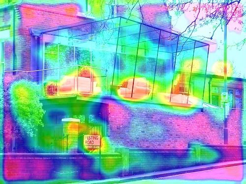
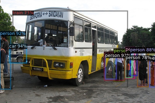
According to the original Faster R-CNN network [28], the unlabeled area in an image would be wrongly treated as background objects in the RPN layer during training. Therefore, the potential unlabeled objects from unseen novel classes are suppressed and hard to be identified as true objects. However, to correct the objectness of these potential objects, the first step is how to find them. We have observed the fact that the network often has clear attention to the potential objects in the RPN layer. As an example, we have used Grad-CAM visualization of the feature map of the RPN layer on some representative training images, as shown in Figure. 2. We observe that although unlabelled novel objects appear in the base training images, the RPN layer could still have strong attention to them, and consequently predict some of them as a known class. In Figure. 2(a) and  2(b), the feature map of $p3$ layer clearly shows the attention of the “chair” (base class) and “sofa” (novel class), but the sofa is predicted to be an instance of the base class “car”. Similarly, in Figure. 2(c) and  2(d), the potential novel objects (“bus”) can also be seen in the feature map of $p4$ layer, and the “bus” is predicted as an instance of the base class “train”. This observation serves as an inspiration to identify potential proposals: some novel objects have high possibilities to be predicted as known base class.

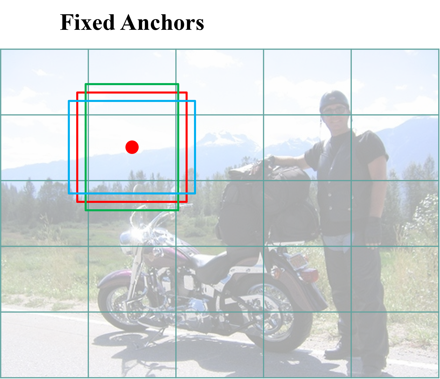
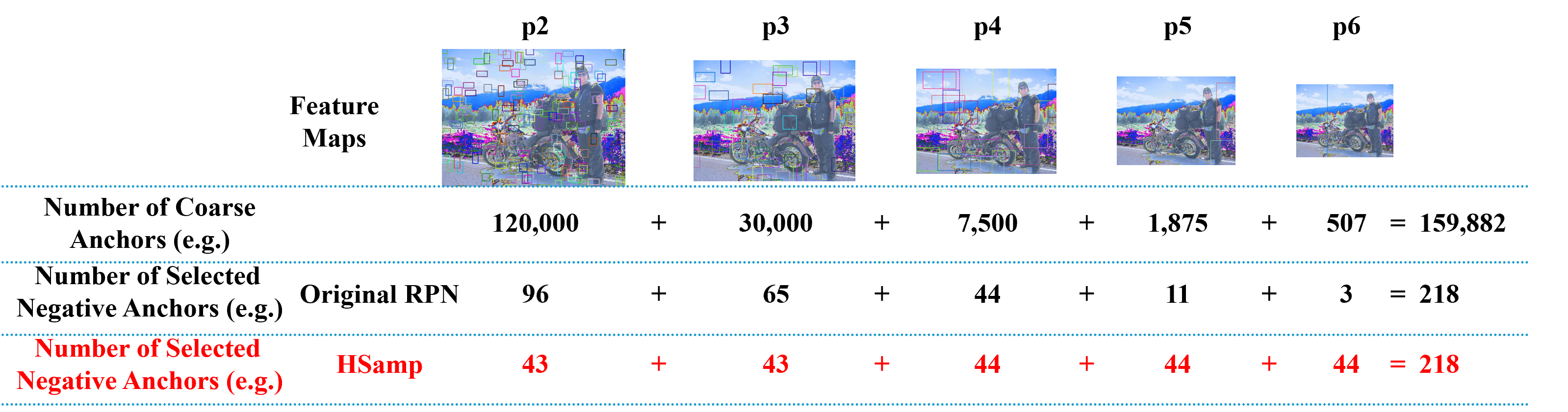
Potential novel unseen class objects that appear in the base class training images usually have lower $iou_{gt}^{a}$  [20] and therefore must be contained by negative anchors ($A_{n}$). Theoretically, there are always exists anchors that can include the potential novel objects in an image. According to the architecture of the RPN layer, anchor boxes are used to determine whether an area contains objects, and each pixel of the feature map will have 3 fixed anchors that are in different sizes and aspect ratios, as shown in Figure. 3(a). Consequently, the overall number of anchors decreases for higher feature maps. In the original RPN layer, different sizes of anchors are applied according to the size of the $p2$ to $p6$ feature maps. Large anchors are more suitable for detecting large objects in high feature layers due to having a larger receptive field, and vice versa. Based on this inch-by-inch sliding window liked search, there should exist a sufficient number of candidates $A_{n}$ such that they contain potential unseen novel objects. However, to improve the training speed, not all of the anchors are used for determining proposal boxes. For an image, only 256 $A_{a}$ and $A_{n}$ anchors among all feature maps are randomly chosen to participate in the RoI pooling. Nonetheless, this random selection process dramatically reduces the chance to get desired negative anchors for large objects in higher feature maps in terms of probability, since the anchors of large size in $p4$ to $p6$ layers intrinsically have fewer cardinal numbers.

(a) End-to-end architecture.

(b) Detailed description of our proposed TernaryHiercRPN.

Figure 5: Our proposed TernaryHiercRPN architecture.

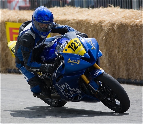
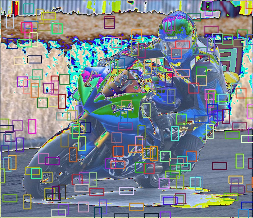
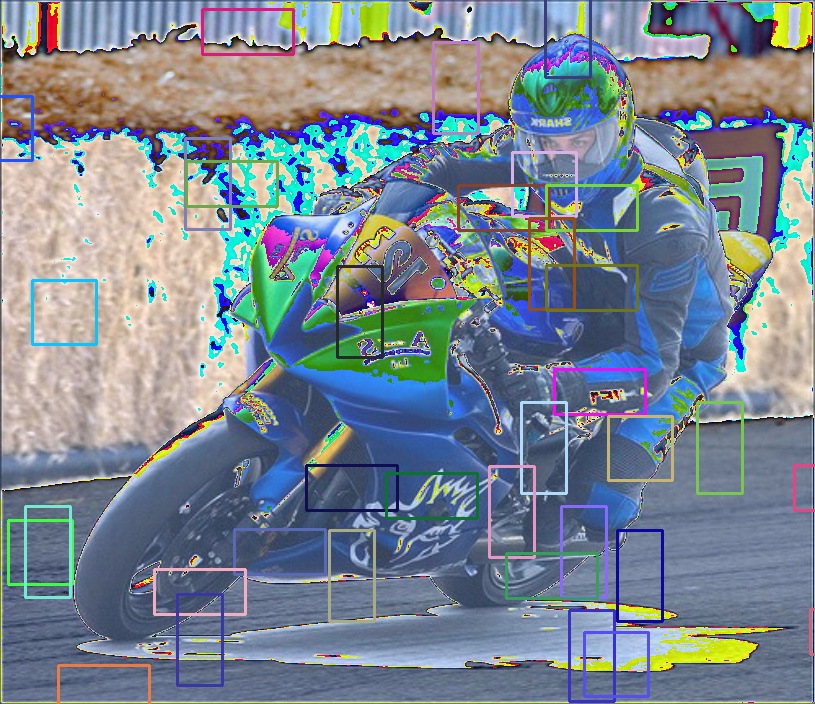
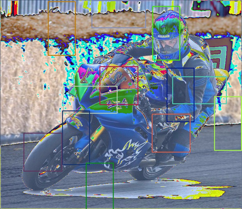
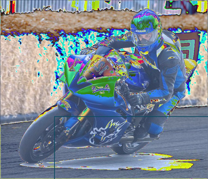
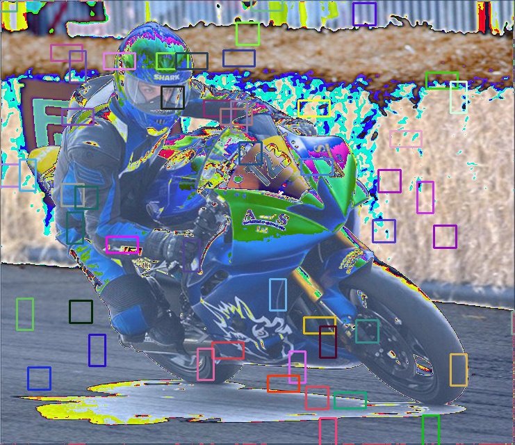
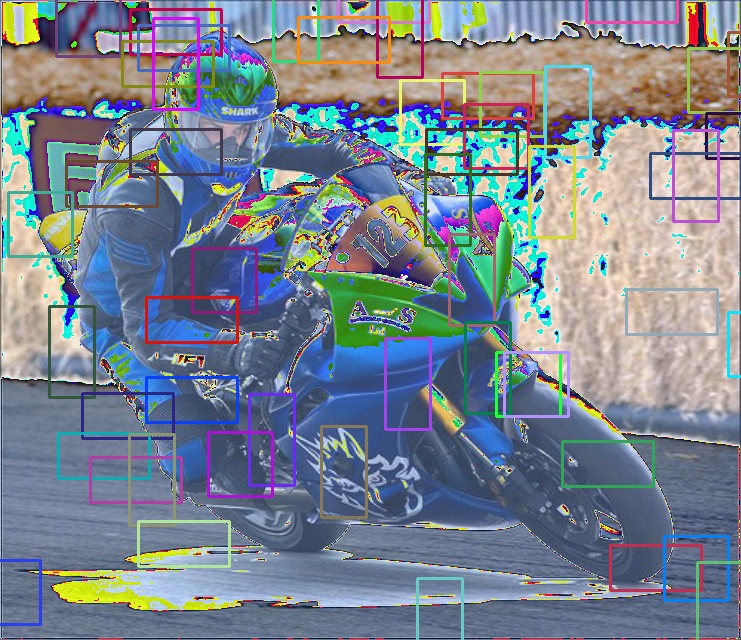
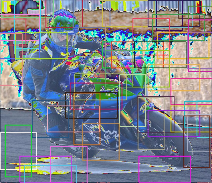
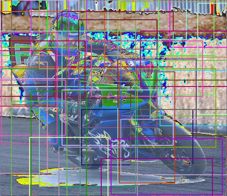
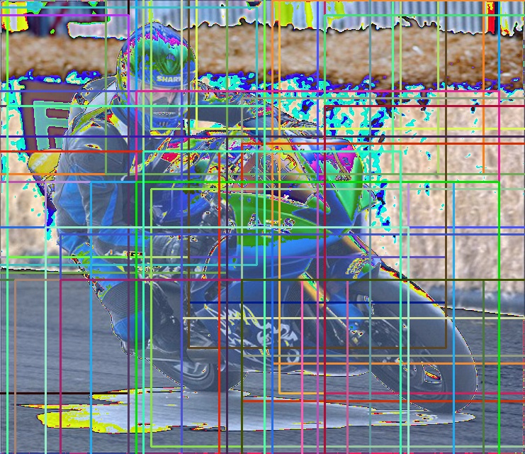
To identify instances of novel unseen classes, we randomly select $A_{n}$s in a hierarchically balanced way, namely hierarchically sampling (HSamp). That is, if we need to pick up $m$ negative anchors ($m\textless 256$), we equally assign them to each feature layer so that each layer will have around $m/5$ anchors. This way, the anchors in each feature layer would share the same possibility for being selected, as shown in Figure. 3(b). Therefore, the anchors that belong to the $p4$ to $p6$ layers are safely preserved. For example, in Figure. 3(b), there are [[120,000], [30,000], [7,500], [1,875], [507]] anchors for $p4$ to $p6$ layers in a training batch, and 218 negative anchors are needed. With the original RPN, these 218 $A_{n}$ anchors are randomly selected which means the number of $A_{n}$ for $p6$ feature map is only 3. In contrast, when HSamp is used, the number of $A_{n}$ is equal for each feature map. We have also visualized the effect of our method in Figure 4. There is hardly any $A_{n}$ that contains the motorbike (novel unseen object) when using the original RPN, as shown in Figure. 4(a) to 4(f). However, when HSamp is used, the chance to have an $A_{n}$ that contains the motorbike is higher, as shown in Figure. 4(g) to 4(l). We conclude that it is crucial to implement a balanced strategy in sampling negative anchors among all feature layers in order to find potential objects that belong to unseen novel classes. The approach will help us to isolate unseen novel class instances as instances that are not similar to the seen classes.

4.2 Hierarchical ternary classification region proposal network (HTRPN)

As mentioned in Section 4.1, faster R-CNN has the ability to recognize a number of potential novel objects that belong to unseen classes, despite the fact that they are unlabelled during training on base class images. We hypothesize that this ability is because of the feature similarity between the features of some novel unseen classes and the base classes. As a result, the model would predict a novel unseen class object as a base class based on its resemblance. In other words, the novel objects contained by the negative anchors could probably have a relatively high classification score towards a base class that resembles them the most. We mark the negative anchors that contain potential novel unseen class objects as potential anchors ($A_{p}$), while others are marked as true negative anchors ($A_{n}^{t}$). Our goal is to distinguish between these two subsets.

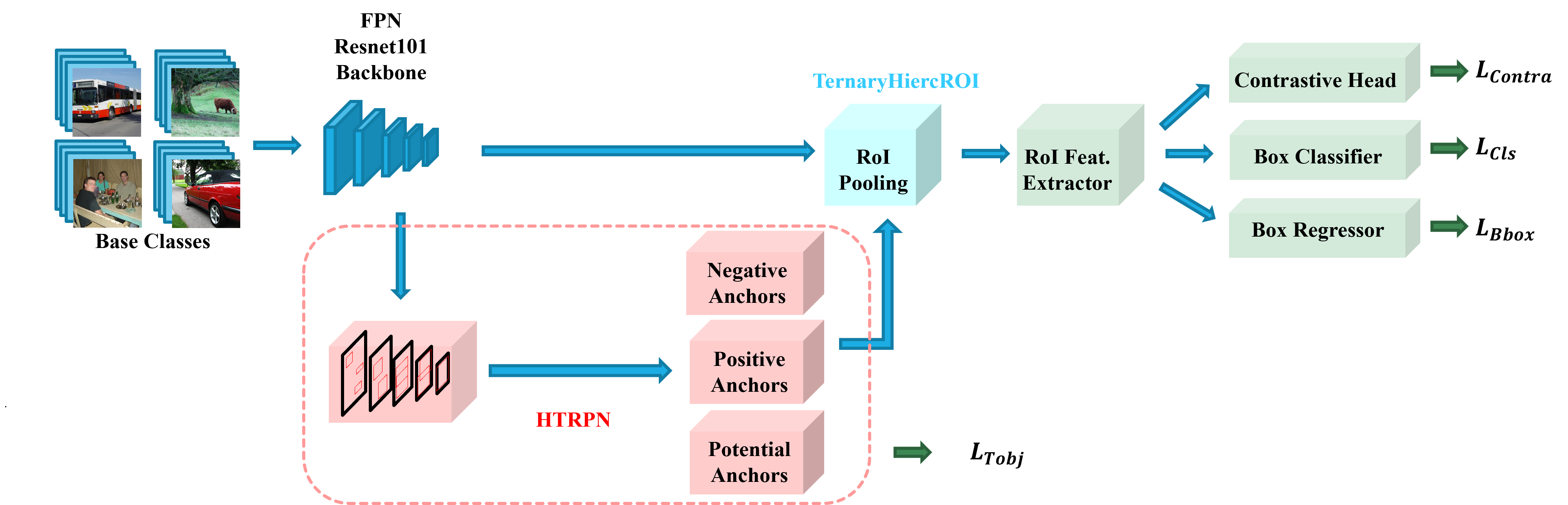
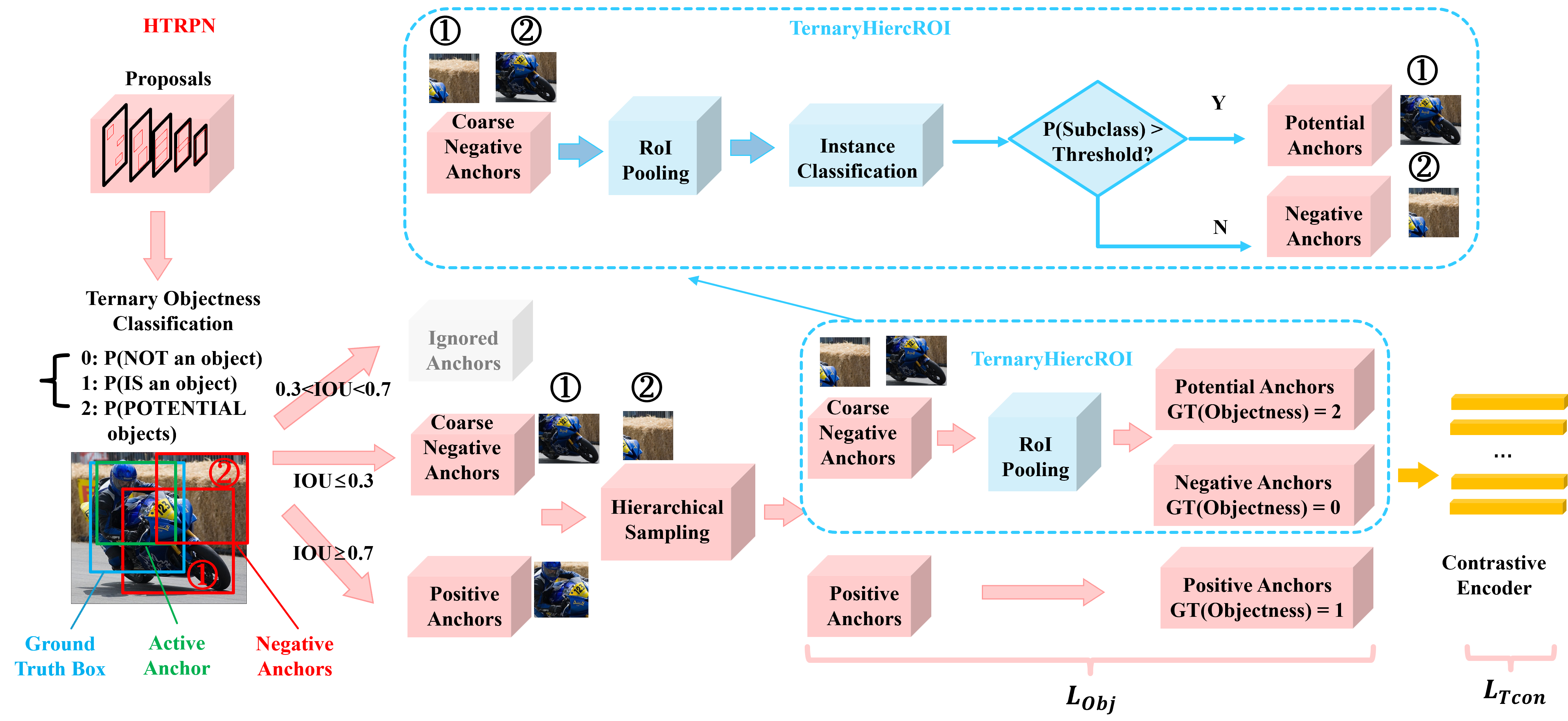
Figure 5 visualizes our proposed architecture for improving FSOD. To better distinguish the set of $A_{p}$ from the set of $A_{n}^{t}$ during training, instead of performing binary classification to determine objectness in the original RPN, we propose a ternary objectness classification (i.e., $tobj\{{tobj_{pre}}^{i},tobj_{gt},iou_{gt}^{a}\}$, where ${tobj_{pre}}^{i}$ are the predicted ternary objectness scores between 0 and 1 for each class $i$; ground-truth value $tobj_{gt}=0$ indicates non-object, $tobj_{gt}=1$ represents a true object, $tobj_{gt}=2$ represents potential objects from unseen novel classes) so that potential objects that belong to unseen novel classes can be classified as a separate class, as visualized in Figure. 5(b). For a training image, after the hierarchical sampling of the coarse negative anchors, we keep these negative anchors for any batch of anchors and perform instance-level sub-classification on them. Here, we set an instance-level classification threshold ($Thre_{cls}$). If we observe that the classification score is larger than the threshold ($P(cls)>Thre_{cls}$) for a base class, then we set the anchor as an objectness-positive anchor, and mark its objectness loss with the ground truth of the label 2. For example the motorbike in Figure. 5(b), the blue box is the ground truth box, active anchors are in green boxes, while negative anchors are in red boxes. Features of the negative anchors are sent to the RoI pooling layer to see if they could be predicted as a visually similar seen category (e.g. the negative anchor ① is predicted as base class “bicycle”, then it is assigned with $tobj_{gt}=2$; but for anchor ② is kept as $tobj_{gt}=0$ since it does not pass the $Thre_{cls}$. We argue that our novel architecture will have a higher FSOD performance.

Figure 6: The 4 blue boxes are the ground truth boxes and the 5 red boxes are the proposals. The proposal ④ contains an unlabeled novel object chair. The top 2 proposals that are ranked by ${tobj_{pre}}^{1}\oplus{tobj_{pre}}^{2}$ could successfully include proposal ④.

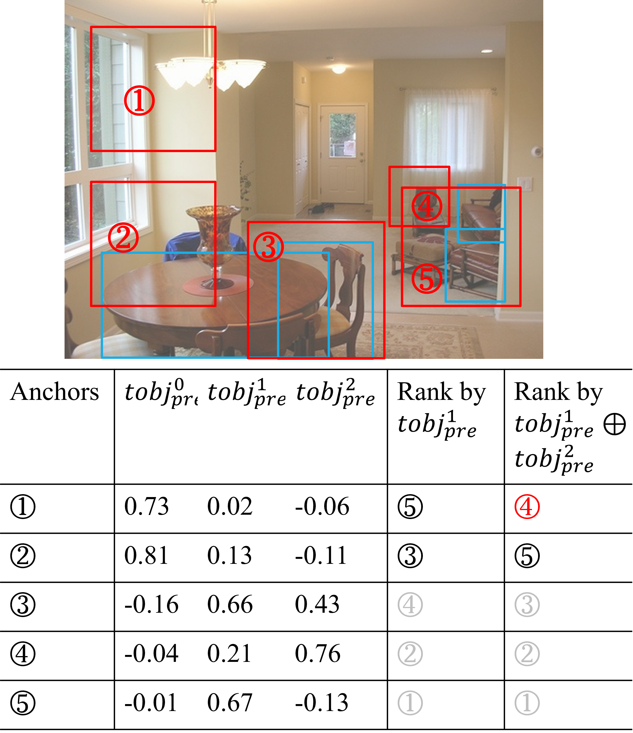
In addition, we need customized solutions for the pre-training and fine-tuning when using our proposed HTRPN. Considering computational resource limitations, only the top 1000 proposals are used for RoI pooling in traditional RPN. Proposals are ranked by their objectness score of ${tobj_{pre}}^{1}$ during the pre-training stage since the model only learns to identify the base classes in this stage. However, in the fine-tuning stage, the ${tobj_{pre}}^{1}$ and ${tobj_{pre}}^{2}$ are both considered for ranking the proposals, because the objectness of some labeled objects might be predicted as ${tobj_{pre}}^{2}$ due to knowledge transfer from the pre-training stage. This step is crucial to realize the objectness consistency because the combination of ${tobj_{pre}}^{1}$ and ${tobj_{pre}}^{2}$ could represent the highly confident proposal and especially improve the possibility of determining positive anchors while inferencing. As shown in Figure 6, if the top two proposals out of the five proposals are ranked only using ${tobj_{pre}}^{1}$, then the proposal ④ would be ignored. However, when the top two proposals are ranked by ${tobj_{pre}}^{1}\oplus{tobj_{pre}}^{2}$ (operator $\oplus$ could be addition or maximum, here we use maximum, details about $\oplus$ will be discussed in Appendix), the proposal ④ could be correctly included. Such a scheme significantly increases the possibility to dig up the true object as much as possible. As a result, the anchors that contain potential novel unseen class objects are well distinguished from the coarse negative anchors. The ternary RPN will let the model maintain its sensitivity to identify new objects from classes that have never been seen before. In practice, not all potential objects that exist in training datasets are going to be singled out during training and only a subset of them could be found. However, these identified novel unseen class objects still can alleviate the confusion of the model during few-shot learning due to their dissimilarity to the seen classes.

4.3 Contrastive learning on objectness

To further increase the inter-class distances between $A_{a}$, $A_{n}^{t}$, and $A_{p}$ subsets in HTRPN, we also include an objectness contrastive learning head (ConsObj) in our architecture. Inspired by the existing literature [31, 16], the cropped features of proposals are sent into an encoder with their ground truth objectness logits to perform contrastive learning. The features of proposals are encoded as a default 128-dimension feature vector, and then the cosine similarity scores are measured between every two proposals. In this way, the HTRPN would give a higher objectness score.

4.4 Training Loss

The global total loss is composed of the classification loss ($\mathcal{L}_{Cls}$), the bounding box regression loss ($\mathcal{L}_{Bbox}$), our ternary objectness loss ($\mathcal{L}_{Tobj}$), and the RoI feature contrastive loss $\mathcal{L}_{Contra}$, as described in Equation. 1. The $\mathcal{L}_{Contra}$ is computed using the contrastive head as described in FSCE  [31]. We set $\alpha=0.5$ to be the fixed weight for balancing the contrastive learning loss.

$$\mathcal{L}=\mathcal{L}_{Cls}+\mathcal{L}_{Bbox}+\mathcal{L}_{Tobj}+\alpha\mathcal{L}_{Contra}$$ (1)

Our proposed ternary objectness loss $\mathcal{L}_{Tobj}$ in Equation. 2 is a sum of the cross entropy objectness loss ($\mathcal{L}_{Obj}$) and ternary RPN feature contrastive learning loss ($\mathcal{L}_{Tcon}$). Similar to $\alpha$ in Equation. 1, $\lambda$ is a balancing factor that is set to be equal 0.5 in our experiments.

$$\mathcal{L}_{Tobj}=\mathcal{L}_{Obj}+\lambda\mathcal{L}_{Tcon}$$ (2)

The ternary RPN contrastive learning loss $\mathcal{L}_{Tcon}$, is defined as an arithmetic mean of the weighted supervised contrastive learning loss $\mathcal{L}_{z_{i}}$ as the following:

$$\mathcal{L}_{Tcon}=\frac{1}{N_{Prop}}\sum_{i=1}^{N_{Prop}}w(iou_{gt}^{p})\cdot\!\mathcal{L}_{z_{i}},$$ (3)

where $N_{Prop}$ represents the number of RPN proposals. Weights $w(iou_{gt}^{p})$ are assigned by the function $g(*)$:

$$w(iou_{gt}^{p})=\mathcal{I}\{iou_{gt}^{p}\geq\phi\}\cdot g(iou_{gt}^{p}),$$ (4)

where $g(*)=1$ is a good hard-clip  [31] and $\mathcal{I}\{*\}$ is a cut-off function that is 1 when $iou_{gt}^{p}\geq\phi\$, otherwise is 0.

$\mathcal{L}_{z_{i}}$ in the RPN proposal contrastive learning loss is given as:

$$\mathcal{L}_{z_{i}}=\!\frac{-1}{N_{obj_{gt}^{i}}\!-\!1}\!\sum_{j=1,j\neq i}^{N_{Prop}}\!\mathcal{I}\{obj_{gt}^{i}=obj_{gt}^{j}\}\cdot\log\!\frac{e^{\tilde{z_{i}}\cdot\!\tilde{z_{j}}\!/\!\tau}}{\sum\limits_{k=1}\limits^{N_{Prop}}\!\mathcal{I}_{k\neq i}\cdot e^{\tilde{z_{i}}\cdot\tilde{z_{k}}/\!\tau}},$$ (5)

where $z_{i}$ denotes the contrastive feature, $obj_{gt}^{i}$ denotes the ground truth ternary objectness label for the $i$-th proposal, $\tilde{z_{i}}$ denotes normalized features while measuring the cosine distances, and $N_{obj_{gt}^{i}}$ denotes the number of proposals with the same objectness label as $obj_{gt}^{i}$.

		Backbone	Split1					Split2					Split3
			1	2	3	5	10	1	2	3	5	10	1	2	3	5	10
LSTD	AAAI 18  [1]	VGG-16	8.2	1.0	12.4	29.1	38.5	11.4	3.8	5.0	15.7	31.0	12.6	8.5	15.0	27.3	36.3
YOLOv2-ft	ICCV19  [37]		6.6	10.7	12.5	24.8	38.6	12.5	4.2	11.6	16.1	33.9	13.0	15.9	15.0	32.2	38.4
RepMet	CVPR 19  [14]	InceptionV3	26.1	32.9	34.4	38.6	41.3	17.2	22.1	23.4	28.3	35.8	27.5	31.1	31.5	34.4	37.2
FRCN-ft	ICCV19  [37]	FRCN-R101	13.8	19.6	32.8	41.5	45.6	7.9	15.3	26.2	31.6	39.1	9.8	11.3	19.1	35.0	45.1
FRCN+FPN-ft	ICML 20  [35]		8.2	20.3	29.0	40.1	45.5	13.4	20.6	28.6	32.4	38.8	19.6	20.8	28.7	42.2	42.1
TFA w/ fc	ICML 20  [35]		36.8	29.1	43.6	55.7	57.0	18.2	29.0	33.4	35.5	39.0	27.7	33.6	42.5	48.7	50.2
TFA w/ cos	ICML 20  [35]		39.8	36.1	44.7	55.7	56.0	23.5	26.9	34.1	35.1	39.1	30.8	34.8	42.8	49.5	49.8
MPSR	ECCV 20  [40]		41.7	-	51.4	55.2	61.8	24.4	-	39.2	39.9	47.8	35.6	-	42.3	48.0	49.7
Retentive R-CNN	CVPR 21  [6]		42.4	45.8	45.9	53.7	56.1	21.7	27.8	35.2	37.0	40.3	30.2	37.6	43.0	49.7	50.1
FSCE	CVPR 21  [31]		44.2	43.8	51.4	61.9	63.4	27.3	29.5	43.5	44.2	50.2	37.2	41.9	47.5	54.6	58.5
TIP	CVPR 21  [18]		27.7	36.5	43.3	50.2	59.6	22.7	30.1	33.8	40.9	46.9	21.7	30.6	38.1	44.5	50.9
DC-Net	CVPR 21  [12]		33.9	37.4	43.7	51.1	59.6	23.2	24.8	30.6	36.7	46.6	32.3	34.9	39.7	42.6	50.7
FSOD-UP	ICCV 21  [38]		43.8	47.8	50.3	55.4	61.7	31.2	30.5	41.2	42.2	48.3	35.5	39.7	43.9	50.6	53.5
CME	CVPR 21  [19]		41.5	47.5	50.4	58.2	60.9	27.2	30.2	41.4	42.5	46.8	34.3	39.6	45.1	48.3	51.5
KFSOD	CVPR 22  [43]		44.6	-	54.4	60.9	65.8	37.8	-	43.1	48.1	50.4	34.8	-	44.1	52.7	53.9
Ours		FRCN-R101	47.0	44.8	53.4	62.9	65.2	29.8	32.6	46.3	47.7	53.0	40.1	45.9	49.6	57.0	59.7

Table 1: The novel classes of nAP50fpr the PASCAL VOC dataset are evaluated on three different category splits with 1 to 10-shot scenarios. The highest score of each few-shot setting is in red color, and the second highest score is in blue color.

5 Experimental Results

We empirically demonstrate that our proposed architecture and training procedure improve the FSOD performance. Our implementation is available as an Appendix.

5.1 Expeiremntal Setup

We use the Faster R-CNN as our object detection model and use ResNet-101 as the backbone along with the feature pyramid network (FPN). The evaluation scheme strictly follows the same paradigm as described in TFA [35]. The mAP50 evaluation results are separately calculated on the base classes (bAP50) and the novel seen class (nAP50). We report our results on the PASCAL VOC and COCO datasets. The contrastive learning head in the fine-tuning stage is computed similarly to FSCE [31]. We used four GPUs for training. The optimizer is fixed as SGD and the weight decay is 1e-4 with momentum as 0.9. We set our batch size equal to 16 for all experiments. The $Thre_{cls}$ is fixed as 0.75. These hyperparameters are not fine-tuned. In the pre-training stage, the top 1000 proposals used for RoI pooling, are ranked by the second objectness logit (is an object). While in the fine-tuning stage, the top 1000 proposals are ranked by the maximum of the second and the third objectness logits (potential object). There are many existing FSOD methods. We compare our performance against a subset of recently developed SOTA FSOD methods.

		Novel AP		Novel AP75
		10	30	10	30
TFA w/ cos	ICML20 [35]	10.0	13.7	9.3	13.4
FSCE	CVPR21 [31]	11.9	16.4	10.5	16.2
SRR-FSD	CVPR21 [44]	11.3	14.7	9.8	13.5
SVD	NeurIPS21 [39]	12.0	16.0	10.4	15.3
FORD+BL	IMAVIS22 [32]	11.2	14.8	10.2	13.9
N-PME	ICASSP22 [23]	10.6	14.1	9.4	13.6
Our		12.1	17.2	11.2	17.1

Table 2: Evaluation on COCO dataset for novel classes for AP and AP75 settings. The highest score of each few-shot setting is in red, and the second highest score is in blue.

5.2 Results on PASCAL VOC

For the PASCAL VOC 2007 and 2012 dataset, 15 categories are chosen as the base classes for pre-training, and the remaining 5 categories served as the novel classes. We follow the 3 different categories splits defined in TFA  [35]. To achieve a fairer comparison, TFA  [35] defined three kinds of combinations of base classes and novel classes, namely split1, split2, and split3. In each split, we evaluate the average precision for novel classes (nAP) on 1,2,3,5,10 shots separately. The training iterations are 8000 for each training epoch. We set the initial learning rate to 0.02. Our results on the three categories splits are reported in Table. 1. We observe that our proposed method reaches new SOTA performance in most cases. Especially, our method is more effective when the $n$-shot is smaller.

5.3 Results on COCO

For the COCO dataset, 60 categories are selected as base classes, and the remaining 20 categories are served as novel classes. The training iterations are set to 20000 during the training stage with an initial learning rate of 0.01. AP for novel classes is evaluated upon $n=10$ and $n=30$ shots separately. Our experiment results for COCO are shown in Table. 2. We again observe that our method outperforms the previous SOTA works in all cases and in some cases the margin of improvement is significant. These experiments demonstrate that our method is effective.

5.4 Ablation Study

Firstly, we discuss the effectiveness of our proposed modules separately, including the Hierarchical sampling of the RPN, the ternary objectness classification, and the contrastive head of the objectness. We implemented the ablation study experiment on PASCAL VOC 5-shot scenario. Each proposed module is added to the original network in an accumulated manner. The results are presented in Table. 3. We observe that all our proposed modules are necessary for optimal performance. By adding the HSamp, we can see that a balanced sampling in RPN is necessary, as it provides comprehensive improvement of $bAP$ and $nAP$ during the pre-training and the fine-tuning stages. We can also observe the results of adding the ternary objectness module indicate that our method will further improve the $nAP$ and do no significant harm to the $bAP$. While the contrastive objectness part demonstrated that it is a simple yet effective way to help build a stronger RPN that could further improve the $bAP$ and $nAP$.

Modules	bAP (pre-trained)	bAP (fine-tuned)	nAP (fine-tuned)
FSCE Baseline*	80.5	68.9	57.2
+ HSamp	80.7	68.9	57.6
+ Ternary Objectness	78.5	67.8	61.9
+ Contrastive Objectness	78.9	68.6	62.9

Table 3: Ablation studies on different modules. The effect of incrementally adding each module to the Baseline network is demonstrated respectively. Sign * represents our reproductive results. We listed the base class mAP50 (bAP) during the pre-training and fine-tuning stage, as well as the novel class mAP50 (nAP) during the fine-tuning stage.

Additionally, we study the influence of different hyperparameter $Thre_{cls}$ settings. We use five $Thre_{cls}$ values from 0.05 to 0.95 for training and record the $nAP$ accordingly, as shown in Table. 4. We observe that for lower $Thre_{cls}$, more candidate potential novel proposals can be distinguished. However, we have lower confidence and consequently lower quality. However, when a higher threshold $Thre_{cls}$ is used, the number of candidates for potential novel proposals is smaller, which is insufficient to optimize objectness in our framework. As the result indicates, $Thre_{cls}=0.75$ is a reasonable value for filtering the candidate proposals relatively well. For additional quantitative analysis please refer to the supplementary materials.

$Thre_{cls}$	0.05	0.25	0.5	0.75	0.95
nAP	60.5	61.2	62.1	62.9	61.4

Table 4: Ablation studies on different hyperparameter settings. The effect of adjusting the $Thre_{cls}$ is demonstrated. The highest nAP has been bolded.

6 Conclusions

We improved the quality FSOD using R-CNN-based architecture via studying the phenomenon of objectness inconsistency due to the potential unlabeled novel objects that belong to unseen classes. By a balance anchor sampling strategy, we enhance the possibility of identifying anchors that may contain objects from unseen classes. In addition, we proposed HTRPN which leads to the recognition ability of potential novel objects and further enhances the objectness consistency. Our method mitigates model confusion about the novel classes and achieves SOTA performance on standard datasets. Future works include extensions to identify novel unseen classes in a zero-shot learning setting.

We include complementary qualitative and quantitative analyses of our method in this Appendix.

Appendix A Ranking proposals

As mentioned in our main paper Section 4.2, the top 1,000 proposals that are most likely to contain objects are selected for the training according to their objectness logit scores. Since our proposed hierarchical ternary region proposal network (HTRPN) has three objectness scores (${tobj_{pre}}^{0}$ indicates the predicted score of non-object, ${tobj_{pre}}^{1}$ represents the score of the true object, ${tobj_{pre}}^{2}$ represents the score of potential objects from unseen novel classes), we rank the proposals by combing their ${tobj_{pre}}^{1}$ and ${tobj_{pre}}^{2}$, mark as ${tobj_{pre}}^{1}\oplus{tobj_{pre}}^{2}$. Operator $\oplus$ could be either arithmetical addition (${tobj_{pre}}^{1}+{tobj_{pre}}^{2}$) or maximum ($max({tobj_{pre}}^{1},{tobj_{pre}}^{2})$).

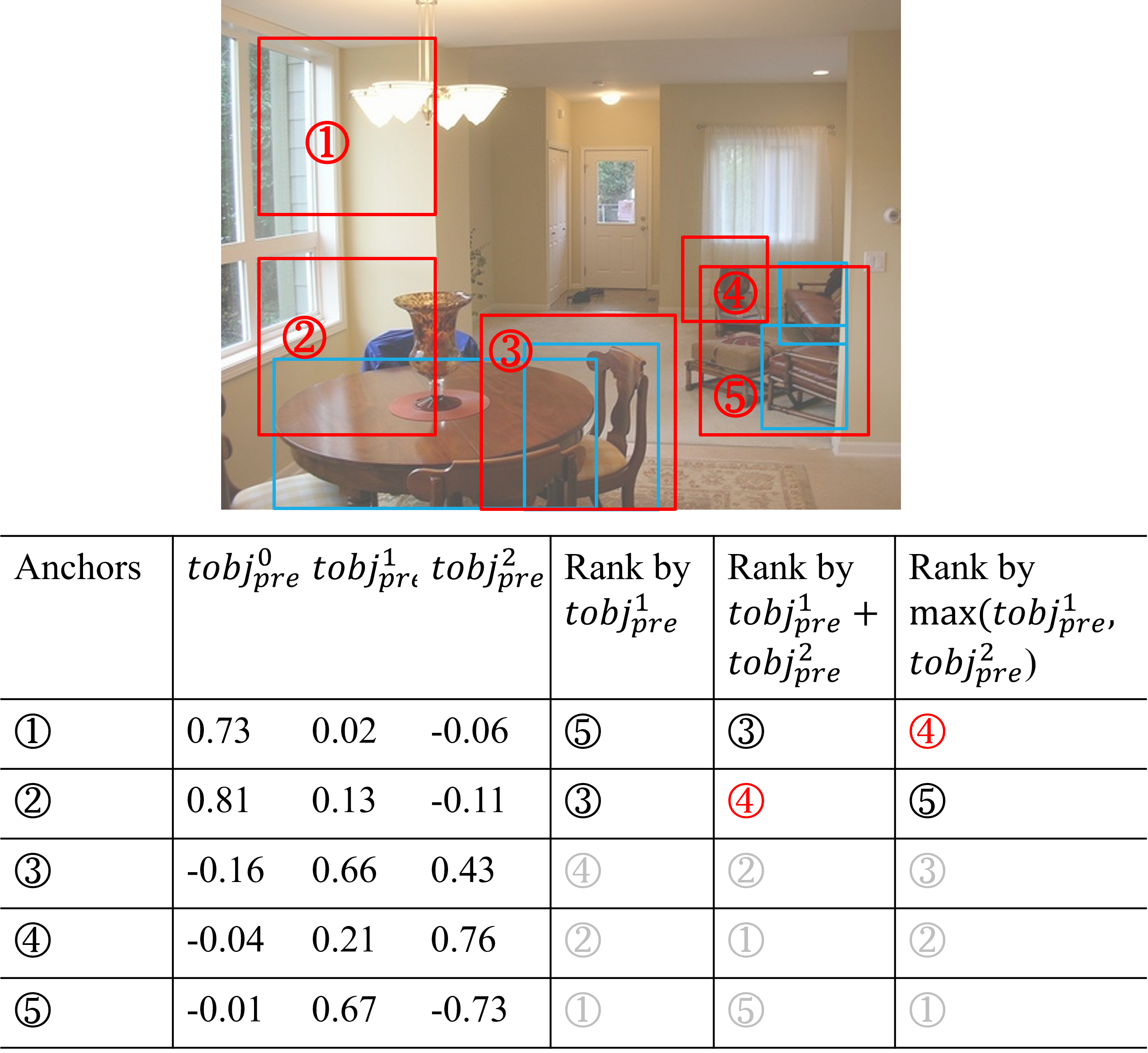
Our examples in Figure. 7 demonstrate the difference between these two types of the operator $\oplus$. In the image, labeled base class objects (tables and chairs) are in blue boxes. For five exemplary proposals ① to ⑤ in red boxes with their ternary objectness logit scores, we intend to pick the top 2 of them. If we rank the proposals only by ${tobj_{pre}}^{1}$, then the proposals that contain unlabeled potential objects (e.g. proposal ④) will more likely be ignored since they are trained to have higher ${tobj_{pre}}^{2}$ score instead of ${tobj_{pre}}^{1}$. Therefore, it is necessary to take the ${tobj_{pre}}^{2}$ score into account, and according to our HTRPN, the objectness of an object should be presented by ${tobj_{pre}}^{1}$ and ${tobj_{pre}}^{2}$ together so that the rank of the potential proposal such as ④ could be significantly promoted. However, by the method of ${tobj_{pre}}^{1}+{tobj_{pre}}^{2}$, the rank of some proposals will be negatively influenced by the negative logit values, such as the proposal ⑤. On the contrary, by applying the maximum between ${tobj_{pre}}^{1}$ and ${tobj_{pre}}^{2}$, the rank of proposal ⑤ will not be degraded by the singular negative values.

Figure 7: The 4 blue boxes are the ground truth boxes and the 5 red boxes are the proposals. The proposal ④ contains an unlabeled novel object chair. The top 2 proposals that are ranked by ${tobj_{pre}}^{1}\oplus{tobj_{pre}}^{2}$ could successfully include proposal ④.

Appendix B Magnitude of potential novel objects

(a) Number of anchors - Training iterations chart of the pre-training stage.

(b) Number of anchors - Training iterations chart of the fine-tuning stage.

Figure 8: The horizontal axis is the training iterations during fine-tuning, and the vertical axis indicates the number of anchors of each training iteration.

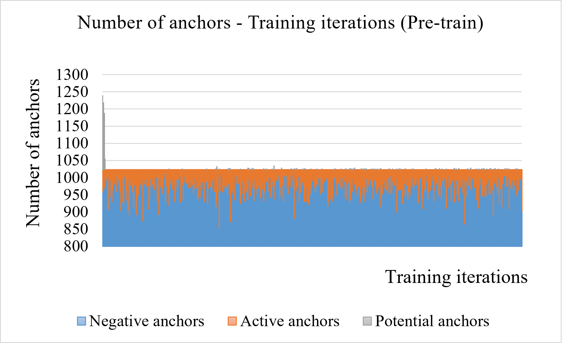
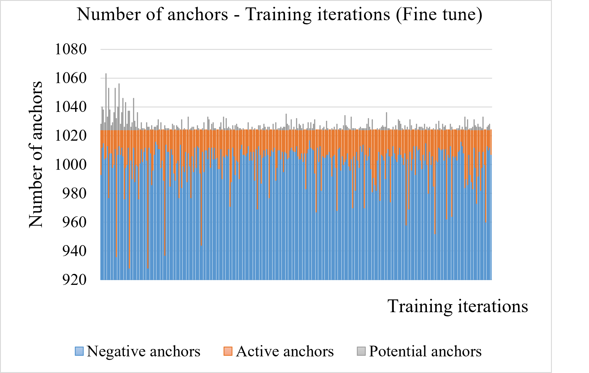
We record the number of potential objects during the pre-training and fine-tuning stages to demonstrate the statistical concept of the potential objects. Our experiments are implemented on the PASCAL VOC dataset with the 5-shot setting. The instance-level ternary classification threshold is fixed as $Thre_{cls}=0.75$. The relation between the number of anchors and the training iteration in the pre-training stage is shown in Figure. 8(a), the overall training anchors for each image is 256, as we claimed in 4.1, thus, for a batch size of 16 on 4 GPUs, the overall training anchors on a single GPU would be around $(16/4)*256=1024$. The negative anchors (blue bars) are the majority, and the number of active anchors (orange bars) is around 0 to 50 for each iteration, which is about 4% of all anchors. However, the number of potential anchors (gray bars) converges with training iterations and stays at around 0 to 5 for each iteration, which indicates our model is getting more stable for recognizing the potential novel objects. Furthermore, as shown in Figure. 8(b), during 5-shot fine-tuning, the trend of the potential anchors is as same as in the pre-training stage. However, when transferring to novel classes, the pre-trained model tends to predict some labeled novel objects as potential novel objects and the beginning of the fine-tuning stage, which could be considered as the inertia of the pre-trained model, therefore, the number of potential anchors is relatively high in the first several iterations of training. This also supports our theory that all true/potential positive ternary objectness of anchors should be presented by the combination of ${tobj_{pre}}^{1}$ and ${tobj_{pre}}^{2}$. And then the number of potential anchors is gradually stabilized to around 0 to 15 for each iteration, which is about 1.5% of all anchors in an iteration.

Hyperparameters	PASCAL VOC	COCO
Learning rate	0.01	0.001
Weight decay	1e-4	1e-4
Optimizer	SGD	SGD
Temperature	0.2	0.2
Contrastie loss weight	0.5	0.5
$Thre_{cls}$	0.75	0.75

Table 5: Hyper parameters that we use for experiments.

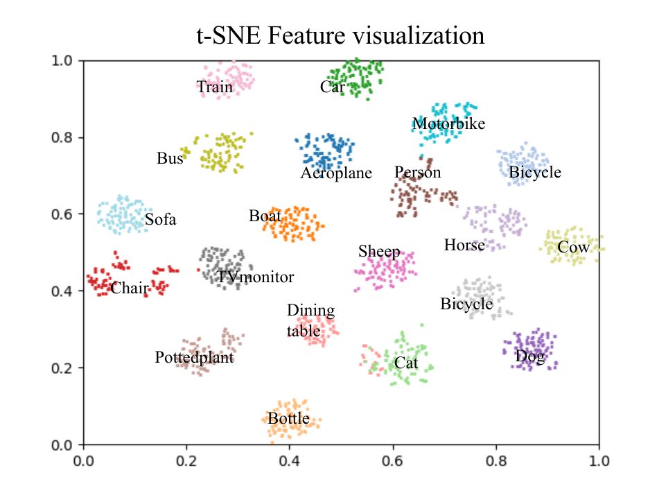
The t-SNE visualized clustering for the 5-shot scenario of the PASCAL VOC dataset is in Figure. 9, each point is an object feature, and the features from the same categories are more likely to form a cluster. A denser cluster indicates a smaller intra-class distance and better recognition ability of its category.

Figure 9: The t-SNE visualization of our HTRPN.

Appendix C Implemented details

We use 4 Nvidia T4 Tensor Core GPUs for both training and evaluation of all datasets. The general hyperparameters we used are listed in Table. 5. As we are applying contrastive learning for RPN and RoI pooling, and the feature space of the pre-training and fine-tuning samples are totally different, the weights of these contrastive learning modules are not transferable from the pre-trained model to the fine-tuning tasks. Therefore, we remove the weights from the pre-trained model for fine-tuning training. The weights from the Resnet backbone and RoI pooling are unfrozen during fine-tuning.

References

- [1] Hao Chen, Yali Wang, Guoyou Wang, and Yu Qiao. LSTD: A low-shot transfer detector for object detection. CoRR, abs/1803.01529, 2018.
- [2] Zewen Chi, Li Dong, Furu Wei, Nan Yang, Saksham Singhal, Wenhui Wang, Xia Song, Xian-Ling Mao, Heyan Huang, and Ming Zhou. Infoxlm: An information-theoretic framework for cross-lingual language model pre-training. arXiv, July 2020.
- [3] Jifeng Dai, Yi Li, Kaiming He, and Jian Sun. R-FCN: object detection via region-based fully convolutional networks. In Daniel D. Lee, Masashi Sugiyama, Ulrike von Luxburg, Isabelle Guyon, and Roman Garnett, editors, Advances in Neural Information Processing Systems 29: Annual Conference on Neural Information Processing Systems 2016, December 5-10, 2016, Barcelona, Spain, pages 379–387, 2016.
- [4] Mark Everingham, Luc Van Gool, Christopher K. I. Williams, John M. Winn, and Andrew Zisserman. The pascal visual object classes (voc) challenge. International Journal of Computer Vision, 88:303–338, 2010.
- [5] Qi Fan, Wei Zhuo, Chi-Keung Tang, and Yu-Wing Tai. Few-shot object detection with attention-rpn and multi-relation detector. In 2020 IEEE/CVF Conference on Computer Vision and Pattern Recognition, CVPR 2020, Seattle, WA, USA, June 13-19, 2020, pages 4012–4021. Computer Vision Foundation / IEEE, 2020.
- [6] Zhibo Fan, Yuchen Ma, Zeming Li, and Jian Sun. Generalized few-shot object detection without forgetting. In Proceedings of the IEEE/CVF Conference on Computer Vision and Pattern Recognition (CVPR), pages 4527–4536, June 2021.
- [7] Hongchao Fang and Pengtao Xie. CERT: contrastive self-supervised learning for language understanding. CoRR, abs/2005.12766, 2020.
- [8] Ross B. Girshick. Fast R-CNN. In 2015 IEEE International Conference on Computer Vision, ICCV 2015, Santiago, Chile, December 7-13, 2015, pages 1440–1448. IEEE Computer Society, 2015.
- [9] Ross B. Girshick, Jeff Donahue, Trevor Darrell, and Jitendra Malik. Rich feature hierarchies for accurate object detection and semantic segmentation. In 2014 IEEE Conference on Computer Vision and Pattern Recognition, CVPR 2014, Columbus, OH, USA, June 23-28, 2014, pages 580–587. IEEE Computer Society, 2014.
- [10] Guangxing Han, Shiyuan Huang, Jiawei Ma, Yicheng He, and S. Chang. Meta faster r-cnn: Towards accurate few-shot object detection with attentive feature alignment. Proceedings of the AAAI Conference on Artificial Intelligence, 36:780–789, 06 2022.
- [11] Guangxing Han, Jiawei Ma, Shiyuan Huang, Long Chen, and Shih-Fu Chang. Few-shot object detection with fully cross-transformer. 2022 IEEE/CVF Conference on Computer Vision and Pattern Recognition (CVPR), pages 5311–5320, 2022.
- [12] Hanzhe Hu, Shuai Bai, Aoxue Li, Jinshi Cui, and Liwei Wang. Dense relation distillation with context-aware aggregation for few-shot object detection. In Proceedings of the IEEE/CVF Conference on Computer Vision and Pattern Recognition (CVPR), pages 10185–10194, June 2021.
- [13] Bingyi Kang, Zhuang Liu, Xin Wang, Fisher Yu, Jiashi Feng, and Trevor Darrell. Few-shot object detection via feature reweighting. In 2019 IEEE/CVF International Conference on Computer Vision, ICCV 2019, Seoul, Korea (South), October 27 - November 2, 2019, pages 8419–8428. IEEE, 2019.
- [14] Leonid Karlinsky, Joseph Shtok, Sivan Harary, Eli Schwartz, Amit Aides, Rogerio Feris, Raja Giryes, and Alex M. Bronstein. Repmet: Representative-based metric learning for classification and few-shot object detection. In Proceedings of the IEEE/CVF Conference on Computer Vision and Pattern Recognition (CVPR), June 2019.
- [15] Prannay Kaul, Weidi Xie, and Andrew Zisserman. Label, verify, correct: A simple few shot object detection method. In Proceedings of the IEEE/CVF Conference on Computer Vision and Pattern Recognition (CVPR), pages 14237–14247, June 2022.
- [16] Prannay Khosla, Piotr Teterwak, Chen Wang, Aaron Sarna, Yonglong Tian, Phillip Isola, Aaron Maschinot, Ce Liu, and Dilip Krishnan. Supervised contrastive learning. CoRR, abs/2004.11362, 2020.
- [17] Mona Kohler, Markus Eisenbach, and Horst Michael Gross. Few-shot object detection: A comprehensive survey. CoRR, abs/2112.11699, 2021.
- [18] Aoxue Li and Zhenguo Li. Transformation invariant few-shot object detection. In Proceedings of the IEEE/CVF Conference on Computer Vision and Pattern Recognition (CVPR), pages 3094–3102, June 2021.
- [19] Bohao Li, Boyu Yang, Chang Liu, Feng Liu, Rongrong Ji, and Qixiang Ye. Beyond max-margin: Class margin equilibrium for few-shot object detection. In Proceedings of the IEEE/CVF Conference on Computer Vision and Pattern Recognition (CVPR), pages 7363–7372, June 2021.
- [20] Yiting Li, Haiyue Zhu, Yu Cheng, Wenxin Wang, Chek Sing Teo, Cheng Xiang, Prahlad Vadakkepat, and Tong Heng Lee. Few-shot object detection via classification refinement and distractor retreatment. In IEEE Conference on Computer Vision and Pattern Recognition, CVPR 2021, virtual, June 19-25, 2021, pages 15395–15403. Computer Vision Foundation / IEEE, 2021.
- [21] Tsung-Yi Lin, Michael Maire, Serge J. Belongie, James Hays, Pietro Perona, Deva Ramanan, Piotr Dollár, and C. Lawrence Zitnick. Microsoft coco: Common objects in context. In European Conference on Computer Vision, 2014.
- [22] Wei Liu, Dragomir Anguelov, Dumitru Erhan, Christian Szegedy, Scott E. Reed, Cheng-Yang Fu, and Alexander C. Berg. SSD: single shot multibox detector. In Bastian Leibe, Jiri Matas, Nicu Sebe, and Max Welling, editors, Computer Vision - ECCV 2016 - 14th European Conference, Amsterdam, The Netherlands, October 11-14, 2016, Proceedings, Part I, volume 9905 of Lecture Notes in Computer Science, pages 21–37. Springer, 2016.
- [23] Weijie Liu, Chong Wang, Shenghao Yu, Chenchen Tao, Jun Wang, and Jiafei Wu. Novel instance mining with pseudo-margin evaluation for few-shot object detection. ICASSP 2022 - 2022 IEEE International Conference on Acoustics, Speech and Signal Processing (ICASSP), pages 2250–2254, 2022.
- [24] Yen-Cheng Liu, Chih-Yao Ma, Zijian He, Chia-Wen Kuo, Kan Chen, Peizhao Zhang, Bichen Wu, Zsolt Kira, and Peter Vajda. Unbiased teacher for semi-supervised object detection. In International Conference on Learning Representations, 2021.
- [25] Xu Luo, Yuxuan Chen, Liangjian Wen, Lili Pan, and Zenglin Xu. Boosting few-shot classification with view-learnable contrastive learning. In 2021 IEEE International Conference on Multimedia and Expo (ICME), pages 1–6, 2021.
- [26] Joseph Redmon, Santosh Kumar Divvala, Ross B. Girshick, and Ali Farhadi. You only look once: Unified, real-time object detection. In 2016 IEEE Conference on Computer Vision and Pattern Recognition, CVPR 2016, Las Vegas, NV, USA, June 27-30, 2016, pages 779–788. IEEE Computer Society, 2016.
- [27] Joseph Redmon and Ali Farhadi. Yolov3: An incremental improvement. CoRR, abs/1804.02767, 2018.
- [28] Shaoqing Ren, Kaiming He, Ross B. Girshick, and Jian Sun. Faster R-CNN: towards real-time object detection with region proposal networks. In Corinna Cortes, Neil D. Lawrence, Daniel D. Lee, Masashi Sugiyama, and Roman Garnett, editors, Advances in Neural Information Processing Systems 28: Annual Conference on Neural Information Processing Systems 2015, December 7-12, 2015, Montreal, Quebec, Canada, pages 91–99, 2015.
- [29] Chuck Rosenberg, Martial Hebert, and Henry Schneiderman. Semi-supervised self-training of object detection models. In 2005 Seventh IEEE Workshops on Applications of Computer Vision (WACV/MOTION’05) - Volume 1, volume 1, pages 29–36, 2005.
- [30] Pierre Sermanet, David Eigen, Xiang Zhang, Michaël Mathieu, Rob Fergus, and Yann LeCun. Overfeat: Integrated recognition, localization and detection using convolutional networks. In Yoshua Bengio and Yann LeCun, editors, 2nd International Conference on Learning Representations, ICLR 2014, Banff, AB, Canada, April 14-16, 2014, Conference Track Proceedings, 2014.
- [31] Bo Sun, Banghuai Li, Shengcai Cai, Ye Yuan, and Chi Zhang. Fsce: Few-shot object detection via contrastive proposal encoding. In Proceedings of the IEEE/CVF Conference on Computer Vision and Pattern Recognition (CVPR), pages 7352–7362, June 2021.
- [32] Anh-Khoa Nguyen Vu, Nhat-Duy Nguyen, Khanh-Duy Nguyen, Vinh-Tiep Nguyen, Thanh Duc Ngo, Thanh-Toan Do, and Tam V. Nguyen. Few-shot object detection via baby learning. Image and Vision Computing, 120:104398, 2022.
- [33] Peng Wang, Kai Han, Xiu-Shen Wei, Lei Zhang, and Lei Wang. Contrastive learning based hybrid networks for long-tailed image classification. In Proceedings of the IEEE/CVF Conference on Computer Vision and Pattern Recognition (CVPR), pages 943–952, June 2021.
- [34] Wenguan Wang, Tianfei Zhou, Fisher Yu, Jifeng Dai, Ender Konukoglu, and Luc Van Gool. Exploring cross-image pixel contrast for semantic segmentation. In 2021 IEEE/CVF International Conference on Computer Vision (ICCV), pages 7283–7293, 2021.
- [35] Xin Wang, Thomas E. Huang, Trevor Darrell, Joseph E Gonzalez, and Fisher Yu. Frustratingly simple few-shot object detection. July 2020.
- [36] Xinya Wang, Jiayi Ma, and Junjun Jiang. Contrastive learning for blind super-resolution via a distortion-specific network. IEEE/CAA Journal of Automatica Sinica, 10(1):78–89, 2023.
- [37] Yu-Xiong Wang, Deva Ramanan, and Martial Hebert. Meta-learning to detect rare objects. In 2019 IEEE/CVF International Conference on Computer Vision (ICCV), pages 9924–9933, 2019.
- [38] Aming Wu, Yahong Han, Linchao Zhu, Yi Yang, and Cheng Deng. Universal-prototype augmentation for few-shot object detection. CoRR, abs/2103.01077, 2021.
- [39] Aming Wu, Suqi Zhao, Cheng Deng, and Wei Liu. Generalized and discriminative few-shot object detection via svd-dictionary enhancement. In NeurIPS, 2021.
- [40] Jiaxi Wu, Songtao Liu, Di Huang, and Yunhong Wang. Multi-scale positive sample refinement for few-shot object detection. In European Conference on Computer Vision, 2020.
- [41] Mengde Xu, Zheng Zhang, Han Hu, Jianfeng Wang, Lijuan Wang, Fangyun Wei, Xiang Bai, and Zicheng Liu. End-to-end semi-supervised object detection with soft teacher. In 2021 IEEE/CVF International Conference on Computer Vision (ICCV), pages 3040–3049, 2021.
- [42] Li Yin, Juan-Manuel Pérez-Rúa, and Kevin J Liang. Sylph: A hypernetwork framework for incremental few-shot object detection. 2022 IEEE/CVF Conference on Computer Vision and Pattern Recognition (CVPR), pages 9025–9035, 2022.
- [43] Shan Zhang, Lei Wang, Naila Murray, and Piotr Koniusz. Kernelized few-shot object detection with efficient integral aggregation. In Proceedings of the IEEE/CVF Conference on Computer Vision and Pattern Recognition (CVPR), pages 19207–19216, June 2022.
- [44] Chenchen Zhu, Fangyi Chen, Uzair Ahmed, Zhiqiang Shen, and Marios Savvides. Semantic relation reasoning for shot-stable few-shot object detection. CoRR, abs/2103.01903, 2021.