CAPE: Camera View Position Embedding for Multi-View 3D Object Detection

Abstract

In this paper, we address the problem of detecting 3D objects from multi-view images. Current query-based methods rely on global 3D position embeddings (PE) to learn the geometric correspondence between images and 3D space. We claim that directly interacting 2D image features with global 3D PE could increase the difficulty of learning view transformation due to the variation of camera extrinsics. Thus we propose a novel method based on CAmera view Position Embedding, called CAPE. We form the 3D position embeddings under the local camera-view coordinate system instead of the global coordinate system, such that 3D position embedding is free of encoding camera extrinsic parameters. Furthermore, we extend our CAPE to temporal modeling by exploiting the object queries of previous frames and encoding the ego motion for boosting $3$D object detection. CAPE achieves the state-of-the-art performance ($61.0\%$ NDS and $52.5\%$ mAP) among all LiDAR-free methods on nuScenes dataset. Codes and models are available.

1 Introduction

3D perception from multi-view cameras is a promising solution for autonomous driving due to its low cost and rich semantic knowledge. Given multiple sensors equipped on autonomous vehicles, how to perform end-to-end 3D perception integrating all features into a unified space is of critical importance. In contrast to traditional perspective-view perception that relies on post-processing to fuse the predictions from each monocular view [44, 43] into the global 3D space, perception in the bird’s-eye-view (BEV) is straightforward and thus arises increasing attention due to its unified representation for 3D location and scale, and easy adaptation for downstream tasks such as motion planning.

The camera-based BEV perception is to predict 3D geometric outputs given the 2D features and thus the vital challenge is to learn the view transformation relationship between 2D and 3D space. According to whether the explicit dense BEV representation is constructed, existing BEV approaches could be divided into two categories: the explicit BEV representation methods and the implicit BEV representation methods. The former constructs an explicit BEV feature map by lifting the 2D perspective-view features to 3D space [19, 33, 12]. The latter mainly follow DETR-based [3] approaches in an end-to-end manner. Without projection or lift operation, those methods [51, 24, 25] implicitly encode the 3D global information into 3D position embedding (3D PE) to obtain 3D position-aware multi-view features, which is shown in Figure 1(a).

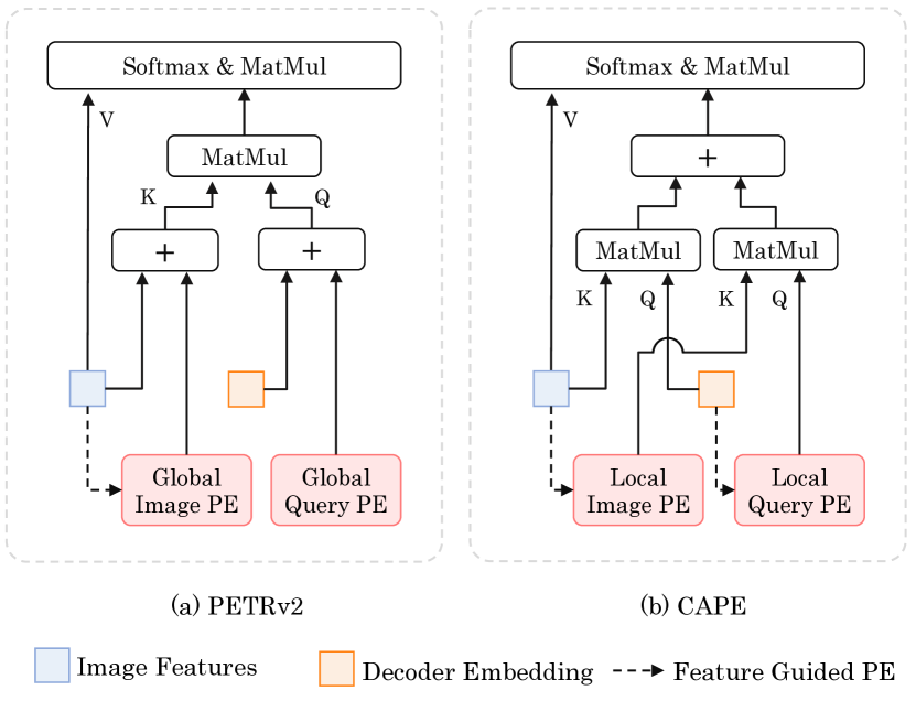
Figure 1: Comparison of the network structure between PETRv2 and our proposed CAPE. (a) In PETRv2, position embedding of queries and keys are in the global system. (b) In CAPE, position embeddings of queries and keys are within the local system of each view. Bilateral cross-attention is adopted to compute attention weights in the local and global systems independently.

Though learning the transformation from 2D images to 3D global space is straightforward, we reveal that the interaction in the global space for the query embeddings and 3D position-aware multi-view features hinders performance. The reasons are two-fold. For one thing, defining each camera coordinate system as the 3D local space, we find that the view transformation couples the 2D image-to-local transformation and the local-to-global transformation together. Thus the network is forced to differentiate variant camera extrinsics in the high-dimensional embedding space for 3D predictions in the global system, while the local-to-global relationship is a simple rigid transformation. For another, we believe the view-invariant transformation paradigm from 2D image to 3D local space is easier to learn, compared to directly transforming into 3D global space. For example, though two vehicles in two views have similar appearances in image features, the network is forced to learn different view transformations, as depicted in Figure 2 (a).

To ease the difficulty in view transformation from 2D image to global space, we propose a simple yet effective approach based on local view position embedding, called CAPE, which performs 3D position embedding in the local system of each camera instead of the 3D global space. As depicted in Figure 2 (b), our approach learns the view transformation from 2D image to local 3D space, which eliminates the variances of view transformation caused by different camera extrinsics.

Specially, as for key 3D PE, we transform camera frustum into 3D coordinates in the camera system using camera intrinsics only, then encoded by a simple MLP layer. As for query 3D PE, we convert the 3D reference points defined in the global space into the local camera system with camera extrinsics only, then encoded by a simple MLP layer. Inspired by  [28, 25], we obtain the 3D PE with the guidance of image features and decoder embeddings, for keys and queries, respectively. Given that 3D PE is in the local space whereas the output queries are defined in the global coordinate system, we adopt the bilateral attention mechanism to avoid the mixture of embeddings in different representation spaces, as shown in Figure 1(b).

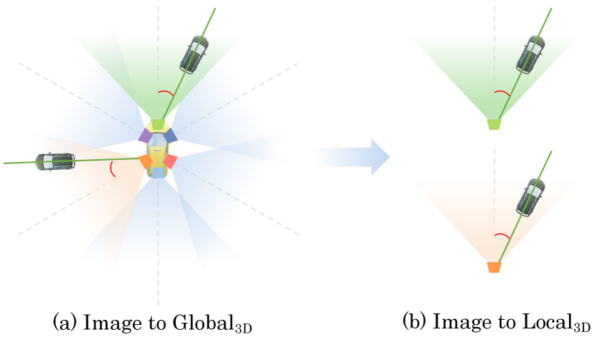
Figure 2: View transformation comparison. In previous methods, view transformation is learned from the image to the global 3D coordinate system directly. In our method, the view transformation is learned from image to local (camera) coordinate system.

We further extend CAPE to integrate multi-frame temporal information to boost the 3D object detection performance, named CAPE-T. Different from previous methods that either warp the explicit BEV features using ego-motion [19, 11] or encode the ego-motion into the position embedding [25], we adopt separated sets of object queries for each frame and encode the ego-motion to fuse the queries.

We summarize our key contributions as follows:

• We propose a novel multi-view 3D detection method, called CAPE, based on camera-view position embedding, which eliminates the variances of view transformation caused by different camera extrinsics.

• We further generalize our CAPE to temporal modeling, by exploiting the object queries of previous frames and leveraging the ego-motion explicitly for boosting 3D object detection and velocity estimation.

• Extensive experiments on the nuScenes dataset show the effectiveness of our proposed approach and we achieve the state-of-the-art among all LiDAR-free methods on the challenging nuScenes benchmark.

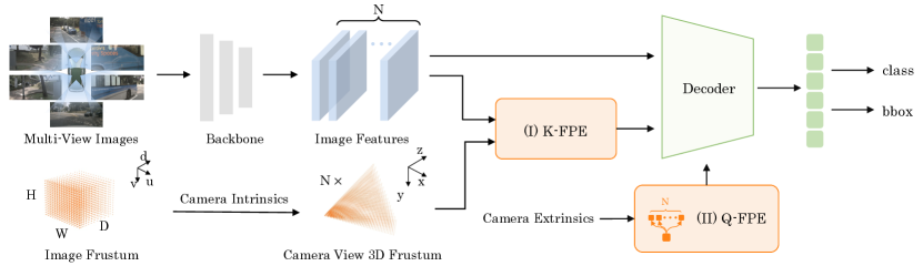
Figure 3: The overview of CAPE. The multi-view images are fed into the backbone network to extract the 2D features including $N$ views. Key position embedding is formed by transforming camera-view frustum points to 3D coordinates in the camera system with camera intrinsics. Images features are used to guide the key position embedding in K-FPE; Query positional embedding is formed by converting the global 3D reference points into $N$ camera-view coordinates with camera extrinsics. Then we encode them under the guidance of decoder embeddings in Q-FPE. The decoder embeddings are updated via the interaction with image features in the decoder. The updated decoder embeddings are used to predict 3D bounding boxes and object classes.

2 Related Work

2.1 DETR-based 2D Detection

DETR  [3] is the pioneering work that successfully adopts transformers [41] in the object detection task. It adopts a set of learnable queries to perform cross-attention and treat the matching process as a set prediction case. Many follow-up methods [52, 5, 47, 22, 15] focus on addressing the slow convergence problem in the training phase. For example, Conditional DETR [28] decouples the items in attention into spatial and content items, which eliminates the noises in cross attention and leads to fast convergence.

2.2 Monocular 3D Detection

Monocular 3D Detection task is highly related to multi-view 3D object detection since they both require restoring the depth information from images. The methods can be roughly grouped into two categories: pure image-based methods and depth-guided methods. Pure image-based methods mainly learn depth information from objects’ apparent size and geometry constraints provided by eight keypoints or pin-hole model  [1, 30, 16, 14, 20, 23, 42, 27]. Depth-guided methods need extra data sources such as point clouds and depth images in the training phase [36, 49, ma2020rethinking, 35, 7]. Pseudo-LiDAR [45] converts pixels to pseudo point clouds and then feeds them into a LiDAR-based detector [39, 26, 49, 8]. DD3D [31] claims that pre-training paradigms could replace the pseudo-lidar paradigm. The quality of depth estimation would have a large influence on those methods.

2.3 Multi-View 3D Detection

Multi-view 3D detection aims to predict 3D bounding boxes in the global system from multi-cameras. Previous methods [44, 43, 4] mostly extend from monocular 3D object detection. Those methods cannot leverage the geometric information in multi-view images. Recently, several methods [38, 37, 33, 10, 19] attempt to percept objects in the global system using explicit bird’s-eye view (BEV) maps. LSS [33] conducts view transform via predicting depth distribution and lift images onto BEV. BEVFormer[19] exploits spatial and temporal information through predefined grid-shaped BEV queries. BEVDepth [18] leverages point clouds as the depth supervision and encodes camera parameters into the depth sub-network.

Some methods learn implicit BEV features following DETR [3] paradigm. These methods mainly initialize 3D sparse object queries and interact with 2D features by attention to directly perform 3D object detection. For example, DETR3D [46] samples 2D features from the projected 3D reference points and then conducts local cross attention to update the queries. PETR [24] proposes 3D position embedding in the global system and then conducts global cross attention to update the queries. PETRv2 [25] extends PETR with temporal modeling and incorporate ego-motion in the position embedding. CAPE conducts the attention in image space and local 3D space to eliminate the variances in view transformation. CAPE could preserve the pros in single-view approaches and leverage the geometric information provided by multi-view images.

2.4 View Transformation

The view transformation from the global view to local view in 3D scenes is an effective approach to boost performances for detection tasks. This could be treated as a normalization by aligning all the views, which could facilitate the learning procedure greatly. Several LiDAR-based 3D detectors [39, 34, 40, 29, 9] estimate local coordinates rather than global coordinates for instances in the second stage, which could fully extract ROI features. For example, PointRCNN [39] proposes the canonical 3D box refinement in the canonical system for more precise regression. To reduce the data variability for point cloud, AziNorm [6] proposes a general normalization in the data pre-process stage. Different from these methods, our method conduct view transformation for eliminating the extrinsic variances brought by multi cameras with camera-view position embedding.

3 Our Approach

We present a camera-view position embedding (CAPE) approach for multi-view 3D detection and construct the position embeddings in each camera coordinate system.

Architecture. We adopt the multi-view DETR framework, a multi-view extension of DETR, depicted in Figure 3. The input multi-view images, $\{\mathbf{I}_{1},\mathbf{I}_{2},\dots,\mathbf{I}_{N}\}$, are processed with the encoders to extract the image embeddings,

$$\mathbf{X}_{n}=\operatorname{Encoder}(\mathbf{I}_{n}).$$ (1)

The $N$ image embeddings are simply concatenated together, $\mathbf{X}=[\mathbf{X}_{1}~{}\mathbf{X}_{2}~{}\dots~{}\mathbf{X}_{N}]$. The associated position embeddings are also concatenated together, $\mathbf{P}=[\mathbf{P}_{1}~{}\mathbf{P}_{2}~{}\dots~{}\mathbf{P}_{N}]$. $\mathbf{X}_{n},\mathbf{P}_{n}\in\mathbb{R}^{C\times I}$, where $I$ is the pixels number.

The decoder is similar to DETR decoder, with a stack of $L$ decoder layers that is composed of self-attention, cross-attention , and feed-forward network (FFN). The $l$-th decoder layer is formulated as follows,

$$\mathbf{O}_{l}=\operatorname{DecoderLayer}(\mathbf{O}_{l-1},\mathbf{R},\mathbf{X},\mathbf{P}).$$ (2)

Here, $\mathbf{O}_{l-1}$ and $\mathbf{O}_{l}$ are the output decoder embedding of the $(l-1)$th and the $l$th layer, respectively. $\mathbf{R}$ are $3$D reference points following the design in [52, 24].

Self-attention is the same as the normal DETR, and takes the sum of $\mathbf{O}_{l-1}$ and the position embedding of the reference points $\mathbf{P}$ as input. Our work lies in learning 3D position embeddings. In contrast to PETR [24] and PETRv2 [25] that form the position embedding in the global coordinate system, we focus on learning position embeddings in the camera coordinate system for cross-attention.

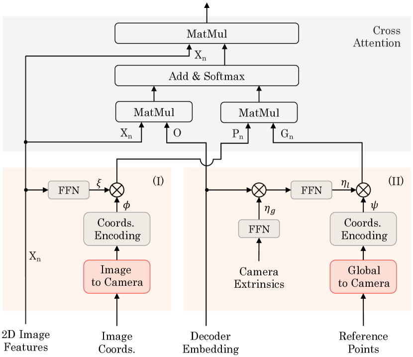
Figure 4: The cross-attention module of CAPE. (I): Feature-guided Key Position Embedding (K-FPE); (II): Feature-guided Query Position Encoder (Q-FPE). The multi-head setting and fully connected layers are omitted for the sake of simplicity.

Key Position Embedding Construction. We take one camera view (one image) as an example and describe how to construct the position embeddings for one view. Each $2$D position in the image plane corresponds to $D$ $3$D coordinates along the predefined depth bins in the frustum: $\{\mathbf{c}_{1},\mathbf{c}_{2},\dots,\mathbf{c}_{D}\}$. The $3$D coordinate in the image frustum is transformed to the camera coordinate system,

$$\mathbf{c}^{\prime}_{d}=\mathbf{T}^{-1}_{i}\mathbf{c}_{d},$$ (3)

where $\mathbf{T}_{i}$ is the intrinsic matrix for $i$-th camera. The $D$ transformed $3$D coordinates $\{\mathbf{c}^{\prime}_{1},\mathbf{c}^{\prime}_{2},\dots,\mathbf{c}^{\prime}_{D}\}$ are mapped into the single embedding,

$$\mathbf{p}=\phi(\mathbf{c}^{\prime}).$$ (4)

Here, $\mathbf{c}^{\prime}$ is a $(D\times 3)$-dimensional vector, with $\mathbf{c}^{\prime}=[{\mathbf{c}^{\prime}}_{1}^{\top}~{}{\mathbf{c}^{\prime}}_{2}^{\top}~{}\dots~{}{\mathbf{c}^{\prime}}_{D}^{\top}]$. $\phi$ is instantiated by a multi-layer perceptron (MLP) of two layers.

Query Position Embedding Construction. We use a set of learnable $3$D reference points $\mathbf{R}=\{\mathbf{r}_{1},\mathbf{r}_{2},\dots,\mathbf{r}_{M}\}$ in the global space to form the object queries. We transform the $M$ $3$D points into the camera coordinate system for each view,

$$\bar{\mathbf{r}}_{nm}=\mathbf{T}_{n}^{e}\mathbf{r}_{m},$$ (5)

where $\mathbf{T}_{n}^{e}$ is the extrinsic parameter matrix for the $n$-th camera denoting the coordinate transformation from the global (LiDAR) system to the camera-view system. The transformed $3$D coordinates are then mapped into the query position embedding,

$$\mathbf{g}_{nm}=\psi(\bar{\mathbf{r}}_{nm}),$$ (6)

where $\psi(\cdot)$ is a two-layer MLP.

Considering that the decoder embedding $\mathbf{O}\in\mathbb{R}^{C\times M}$ and query position embeddings are about different coordinate systems: global coordinate system and camera view coordinate system, respectively, we form the camera-dependent decoder queries through concatenation(denote as $[\cdot]$):

$$\mathbf{Q}_{n}=[\mathbf{O}^{\top}~{}\mathbf{G}_{n}^{\top}]^{\top},$$ (7)

where $\mathbf{G}_{n}=[\mathbf{g}_{n1}\mathbf{g}_{n2}\dots\mathbf{g}_{nM}]\in\mathbb{R}^{C\times M}$. Accordingly, the keys for cross-attention between queries and image features are also formed through concatenation, $\mathbf{K}_{n}=[\mathbf{X}_{n}^{\top}~{}\mathbf{P}_{n}^{\top}]^{\top}$. The $n-$view pre-normalized cross-attention weights $\mathbf{W}_{n}\in\mathbb{R}^{I\times M}$ is computed from:

$$\mathbf{W}_{n}=\mathbf{K}_{n}^{\top}\mathbf{Q}_{n}=\mathbf{X}_{n}^{\top}\mathbf{O}+\mathbf{P}_{n}^{\top}\mathbf{G}_{n}$$ (8)

The decoder embedding is updated by aggregating information from all views:

$$\mathbf{O}\xleftarrow{}{}\sum_{n}\mathbf{X}_{n}\sigma(\mathbf{W}_{n}),$$ (9)

where $\sigma$ is the soft-max, note that projection layers are omitted for simplicity. More details can be seen in the appendix. Feature-guided Key and Query Position Embeddings. Similar to PETRv2 [25], we make use of the image features to guide the key position embedding computation by learning the scaling weights and update Eq.4 as:

$$\mathbf{p}=\phi(\mathbf{c}^{\prime})\odot\xi(\mathbf{x}),$$ (10)

where $\xi(\cdot)$ is a two-layers MLP, $\odot$ denotes the element-wise multiplication and $\mathbf{x}$ is the image features at the corresponding position. It is assumed to provide some informative guidance (e.g., depth).

On the query side, inspired by conditional DETR [28], we use the decoder embedding to guide the query position embedding computation and update Eq.6 as:

$$\mathbf{g}_{nm}=\psi(\bar{\mathbf{r}}_{nm})\odot\eta(\mathbf{o}_{m},\mathbf{T}_{n}^{e}).$$ (11)

The extrinsic parameter matrix $\mathbf{T}_{n}^{e}$ is used to transform the spatial decoder embedding $\mathbf{o}_{m}$ to camera coordinate system, for alignment with the reference point position embeddings. Specifically, $\eta(\cdot)$ is instantiated as:

$$\eta(\mathbf{o}_{m},\mathbf{T}_{n}^{e})=\eta_{l}(\mathbf{o}_{m}\odot\eta_{g}(\mathbf{T}_{n}^{e})).$$ (12)

Here $\eta_{l}(\cdot)$ and $\eta_{g}(\cdot)$ are two-layers MLP.

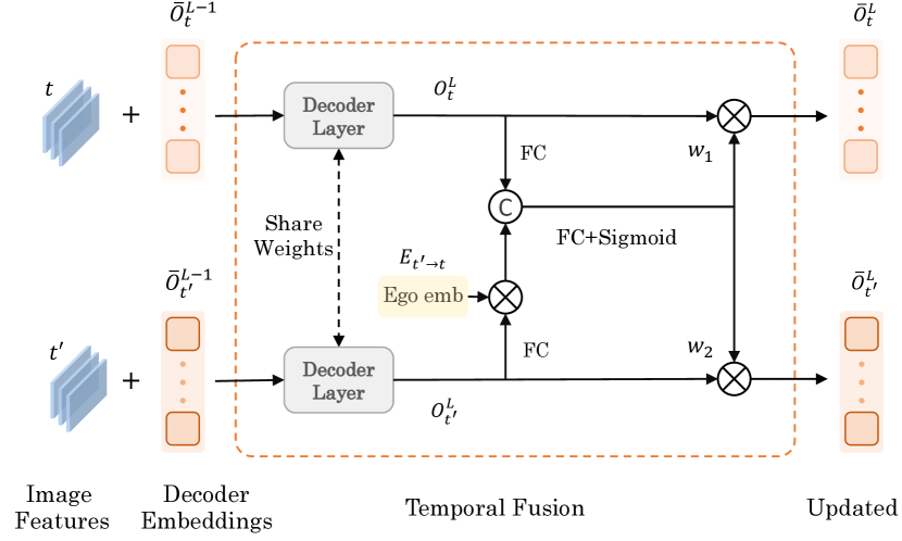
Figure 5: The pipeline of our temporal modeling. The ego-motion embedding modulates the decoder embedding for spatial alignment. Then each decoder embedding is scaled by the attention weights $(w1,w2)$ that predicted from the aligned embeddings.

Temporal modeling with ego-motion embedding. We utilize the previous frame information to boost the detection for the current frame. The reference points of the previous frame are transformed from the reference points of the current frame using the ego-motion matrix $\mathbf{M}$,

$$\mathbf{R}_{t^{\prime}}=\mathbf{M}\mathbf{R}_{t}.$$ (13)

Considering the same moving objects may have different 3D positions in two frames, we build the separated decoder embeddings $(\mathbf{O}_{t},\mathbf{O}_{t^{\prime}})$ that can represent different position information for each frame. The interaction between the decoder embeddings of two frames for $l$-th decoder layer is formulated as follows:

$$(\bar{\mathbf{O}}_{t}^{L},\bar{\mathbf{O}}_{t^{\prime}}^{L})=f(\mathbf{O}_{t}^{L},\mathbf{O}_{t^{\prime}}^{L},\mathbf{M}).$$ (14)

We elaborate on the interaction between queries in two frames in Figure 5. Given that $\mathbf{O}_{t}$ and $\mathbf{O}_{t^{\prime}}$ are not in the same ego coordinate system, we inject the ego-motion information into the decoder embedding $\mathbf{O}_{t^{\prime}}$ for spatial alignment. Then we update decoder embeddings with channel attention weights generated from the concatenation of the decoder embeddings of two frames. Compared with using one set of queries learning objects in different frames, queries in our method have a stronger capability in positional learning.

Heads and Losses. The detection heads consist of the classification branch that predicts the probability of object classes and the regression branch that regresses 3D bounding boxes. The regression branch predicts the relative offsets w.r.t. the coordinates of 3D reference points in the global system. As for the loss function, we adopt focal loss [21] for classification $L_{cls}$ and L1 loss for regression $L_{reg}$ following prior works [46, 24]. The label assignment strategy here is the Hungarian algorithm [13]. Suppose that $\sigma$ is the assignment function, the loss for 3D object detection for the model without temporal modeling can be summarized as:

$$\begin{gathered}L_{cur}(\mathbf{y},\mathbf{\hat{y}})=\lambda_{cls}L_{cls}(\mathbf{c},\sigma{(\mathbf{\hat{c})}})+L_{reg}(\mathbf{b},\sigma{(\mathbf{\hat{b}})}),\end{gathered}$$ (15)

where $\mathbf{y}=(\mathbf{c},\mathbf{b})$ and $\hat{\mathbf{y}}=(\mathbf{\hat{c}},\mathbf{\hat{b}})$ denote the set of ground truths and predictions respectively. $\lambda_{cls}$ is a hyper-parameter to balance losses. As for the network with temporal modeling, different from other methods supervise predictions only on the current frame, we predict results and supervise them on previous frames as auxiliary losses to enhance the temporal consistency. We use the center location and velocity of the ground truth on the current frame to generate the ground truths on the previous frame.

$$\begin{gathered}L_{all}=L_{cur}+\lambda L_{prev}.\end{gathered}$$ (16)

$L_{cur}$ and $L_{prev}$ denote the losses for the current and previous frame separately. $\lambda$ is a hyper-parameter to balance losses.

4 Experiments

4.1 Dataset

We evaluate CAPE on the large-scale nuScenes [2] dataset. This dataset is composed of 1000 scene videos, with 700/150/150 scenes for training, validation, and testing set, respectively. Each sample consists of RGB images from 6 cameras and has 360 ° horizontal FOV. There are 20s video frames for each scene and 3D annotations are provided with every 0.5s. We report nuScenes Detection Score (NDS), mean Average Precision (mAP), and five True Positive (TP) metrics: mean Average Translation Error (mATE), mean Average Scale Error (mASE), mean Average Orientation Error (mAOE), mean Average Velocity Error (mAVE), mean Average Attribute Error (mAAE).

4.2 Implementation Details

We follow the PETR [24] to report the results. We stack six transformer layers and adopt eight heads in the multi-head attention. Following other methods[24, 46, 12], CAPE is trained with the pre-trained model FCOS3D [44] on validation dataset and with DD3D [31] pre-trained model on the test dataset as initialization. We use regular cropping, resizing, and flipping as data augmentations. The total batch size is eight, with one sample per GPU. We set $\lambda$ = 0.1 to balance the loss weight between the current frame and the previous frame and set $\lambda_{cls}$ = 2.0 to balance the loss weight between classification and regression. For validation dataset setting, we train CAPE for 24 epochs on 8 A100 GPUs with a starting learning rate of 2$e^{-4}$ that decayed with cosine annealing policy. For test dataset setting, we adopt denoise [50] for faster convergence. We train 24 epochs with CBGS on the single-frame setting. Then we load the single-frame model of CAPE as the pre-trained model for multi-frame training of CAPE-T and train 60 epochs without CBGS.

Table 1: Comparison of recent works on the nuScenes test set. $\ddagger$ is test time augmentation. Setting “S”: only using single-frame information, “M”: using multi-frame (two) information. “L”: using extra LiDAR data source as depth supervision.

Methods	Year	Backbone	Setting	NDS$\uparrow$	mAP$\uparrow$	mATE$\downarrow$	mASE$\downarrow$	mAOE$\downarrow$	mAVE$\downarrow$	mAAE$\downarrow$
BEVDepth‡ [18]	arXiv2022	V2-99	M, L	0.600	0.503	0.445	0.245	0.378	0.320	0.126
BEVStereo‡ [17]	arXiv2022	V2-99	M, L	0.610	0.525	0.431	0.246	0.358	0.357	0.138
FCOS3D‡ [44]	ICCV2021	Res-101	S	0.428	0.358	0.690	0.249	0.452	1.434	0.124
PGD‡ [43]	CoRL2022	Res-101	S	0.448	0.386	0.626	0.245	0.451	1.509	0.127
DETR3D [46]	CoRL2022	Res-101	S	0.479	0.412	0.641	0.255	0.394	0.845	0.133
BEVDet‡ [12]	arXiv2022	V2-99	S	0.488	0.424	0.524	0.242	0.373	0.950	0.148
PETR [24]	ECCV2022	V2-99	S	0.504	0.441	0.593	0.249	0.383	0.808	0.132
CAPE	-	V2-99	S	0.520	0.458	0.561	0.252	0.389	0.758	0.132
BEVFormer [19]	ECCV2022	V2-99	M	0.569	0.481	0.582	0.256	0.375	0.378	0.126
BEVDet4D‡ [11]	arXiv2022	Swin-B	M	0.569	0.451	0.511	0.241	0.386	0.301	0.121
PETRv2 [25]	arXiv2022	V2-99	M	0.582	0.490	0.561	0.243	0.361	0.343	0.120
CAPE-T	-	V2-99	M	0.610	0.525	0.503	0.242	0.361	0.306	0.114

Table 2: Comparison on the nuScenes validation set with large backbones. All listed methods are trained with 24 epochs without CBGS.

Methods	Backbone	Resolution	Setting	NDS$\uparrow$	mAP$\uparrow$	mATE$\downarrow$	mASE$\downarrow$	mAOE$\downarrow$	mAVE$\downarrow$	mAAE$\downarrow$
BEVDet [12]	Swin-B	$1408\times 512$	S	0.417	0.349	0.637	0.269	0.490	0.914	0.268
PETR [24]	V2-99	$1600\times 900$	S	0.455	0.406	0.736	0.271	0.432	0.825	0.204
CAPE	V2-99	$1600\times 900$	S	0.479	0.439	0.683	0.267	0.427	0.814	0.197
BEVDet4D [11]	Swin-B	$1600\times 900$	M	0.515	0.396	0.619	0.260	0.361	0.399	0.189
PETRv2 [25]	V2-99	$800\times 320$	M	0.503	0.410	0.723	0.269	0.453	0.389	0.193
CAPE-T	V2-99	$800\times 320$	M	0.536	0.440	0.675	0.267	0.396	0.323	0.185

Table 3: Comparison on the nuScenes validation set with ResNet backbone. “†”: the results are reproduced for a fair comparison with our method(trained with 24 epochs).

Method	Backbone	Resolution	CBGS	NDS$\uparrow$	mAP$\uparrow$
PETR† [24]	Res-50	$1408\times 512$	✗	0.367	0.317
CAPE	Res-50	$1408\times 512$	✗	0.380	0.337
FCOS3D [44]	Res-101	$1600\times 900$	✓	0.415	0.343
PGD [43]	Res-101	$1600\times 900$	✓	0.428	0.369
DETR3D [46]	Res-101	$1600\times 900$	✓	0.434	0.349
BEVDet [12]	Res-101	$1056\times 384$	✓	0.396	0.330
PETR [24]	Res-101	$1600\times 900$	✓	0.442	0.370
CAPE	Res-101	$1600\times 900$	✓	0.463	0.388
BEVFormer [19]	Res-50	$800\times 450$	✗	0.354	0.252
PETRv2† [25]	Res-50	$704\times 256$	✗	0.402	0.293
CAPE-T	Res-50	$704\times 256$	✗	0.442	0.318
BEVFormer [19]	Res-101	$1600\times 640$	✓	0.517	0.416
PETRv2 [25]	Res-101	$1600\times 640$	✓	0.524	0.421
CAPE-T	Res-101	$1600\times 640$	✓	0.533	0.431

4.3 Comparison with State-of-the-art

We show the performance comparison in the nuScenes test set in Tab. 1. We first compare the CAPE with state-of-the-art methods on the single-frame setting and then compare CAPE-T(the temporal version of CAPE) with methods that leverage temporal information. As for the model on the single-frame setting, as far as we know, CAPE(NDS=52.0) could achieve the first place on nuScenes benchmark compared with vision-based methods with the single-frame setting. As for the model with temporal modeling, CAPE-T still outperforms all listed methods. CAPE achieves $61.0\%$ on NDS and $52.5\%$ on mAP. We point out that using LiDAR as supervision could largely improve the mATE metric, thus it’s not fair to compare methods (w/wo LiDAR supervision) together. Nevertheless, even compared with contemporary methods leveraging LiDAR as supervision, CAPE outperforms BEVDepth [18] $1.0\%$ on NDS and $2.2\%$ on mAP and achieves comparable results to BEVStereo [17].

We further show the performance comparison on the nuScenes validation set in Tab. 2 and Tab. 3. It could be seen that CAPE surpasses our baseline to a large margin and performs well compared with other methods.

4.4 Ablation Studies

In this section, we validate the effectiveness of our designed components in CAPE. We use the $1600\times 900$ resolution for all single-frame experiments and the $800\times 320$ resolution for all multi-frames experiments.

Effectiveness of camera view position embedding. We validate the effectiveness of our proposed camera view position embedding in Tab 4. In Setting(a), we simply adopt PETR with feature-guided position embedding as our baseline. When we adopt the bilateral attention mechanism with 3D position embedding in the LiDAR system in Setting(b), the performance can be improved by $0.5\%$ on NDS. When using camera 3D position embedding without bilateral attention mechanism in Setting(c), the model could not converge and only get $2.5\%$ NDS. It indicates that the 3D position embedding in the camera system should be decoupled with output queries in the LiDAR system. The best performances could be achieved when we use camera view position embeddings along with the bilateral attention mechanism. For fair comparison with 3D position embedding in the LiDAR system, camera view position embedding improves $1.4\%$ in NDS and $2.4\%$ in mAP (see Setting(b) and (d)).

Table 4: Ablation study of camera view position embedding and bilateral attention mechanism on the nuScenes validation set. “Cam.View”: 3D position embeddings are constructed in the camera system, otherwise 3D position embeddings are constructed in the global (LiDAR) system.“Bilateral”: bilateral attention mechanism is adopted in the decoder.

Setting	Cam.View	Bilateral	NDS$\uparrow$	mAP$\uparrow$	mATE$\downarrow$	mAOE$\downarrow$
(a)			0.460	0.409	0.734	0.424
(b)		$\checkmark$	0.465	0.415	0.708	0.420
(c)	$\checkmark$		0.025	0.100	1.117	0.918
(d)	$\checkmark$	$\checkmark$	0.479	0.439	0.683	0.427

Table 5: Ablation study of feature guided position embedding in queries and keys on the nuScenes validation set. “Q-FPE”: using feature-guided design in queries.“K-FPE”: using feature-guided design in keys.

Setting	Q-FPE	K-FPE	NDS$\uparrow$	mAP$\uparrow$	mATE$\downarrow$	mAOE$\downarrow$
(a)			0.447	0.415	0.719	0.515
(b)	$\checkmark$		0.449	0.421	0.693	0.551
(c)		$\checkmark$	0.463	0.420	0.700	0.473
(d)	$\checkmark$	$\checkmark$	0.479	0.439	0.683	0.427

Effectiveness of feature-guided position embedding. Tab. 5 shows the effect of feature-guided position embedding in both queries and keys. Different from the FPE in PETRv2[32], our K-FPE here is formed under the local camera-view coordinate system instead of the global coordinate system. Compared with Setting(a) and (b), we find the Q-FPE increases the location accuracy (see the improvement of mAP and mATE), but decreases the orientation performance in mAOE, mainly owing to the lack of image appearance information in the local view attention. Compared with Setting(a) and (c), using K-FPE could improve $1.6\%$ on NDS and $4.2\%$ on mAOE, which benifits from more precise depth and orientation information in image appearance features. Compared with Setting(c) and (d), adding Q-FPE could bring $1.6\%$ and $1.9\%$ gain on NDS and mAP further. The benefit brought by Q-FPE could be explained by 3D anchor points being refined by input queries in high-dimensional embedding space. It could see that using both Q-FPE and K-FPE achieves the best performances.

Effectiveness of the temporal modeling approach. We show the necessity of using a set of queries for each frame in Tab. 6. It could be observed that decomposing queries into different frames could improve $0.9\%$ on NDS and $0.8\%$ on mAP. With the multi-group design, one object query could correspond to one instance on each frame respectively, which is proper for DETR-based paradigms. Similar conclusion is also observed in 2D instance segmentation tasks [48]. Since we use multi groups of queries, auxiliary supervision on previous frames can be added to better align object queries between frames. Meanwhile, the generated ground truth on the previous frame could be treated as a type of data augmentation to avoid overfitting. When we adopt the previous loss, the mAP increases $0.5\%$, which proves the validity of supervision on multi-frames. Compared with Setting(a) and (c), our temporal modeling approach could improve $1.4\%$ on NDS and $1.2\%$ on mAP on the validation dataset.

Table 6: Ablation studies of our temporal modeling approach with ego-motion embedding on the nuScenes validation set. We validate the necessity of using a group of queries for each frame and the effectiveness of conducting the supervision on previous frames. “QT”: whether sharing Queries for each frame in Temporal modeling. “LP”: using auxiliary Loss on Previous frames.

Setting	QT	LP	NDS$\uparrow$	mAP$\uparrow$	mAOE$\downarrow$	mAVE$\downarrow$
(a)	Share		0.522	0.428	0.454	0.341
(b)	Not Share		0.531	0.436	0.401	0.346
(c)	Not Share	$\checkmark$	0.536	0.440	0.396	0.323

Table 7: Ablation study of our temporal fusion approach on nuScenes validation set. “Ego”: using ego motion embedding in the fusion process; “concat + ML”: simply concatenating queries in two frames and using a two-layer MLP to output fused queries; “channel att”: learning channel attention weights for each query.

Setting	Fusion ways	Ego	NDS$\uparrow$	mAP$\uparrow$	mAOE$\downarrow$	mAVE$\downarrow$
(a)	concat + MLP		0.527	0.432	0.413	0.343
(b)	concat + MLP	$\checkmark$	0.531	0.439	0.432	0.318
(c)	channel att		0.530	0.432	0.400	0.333
(d)	channel att	$\checkmark$	0.536	0.440	0.396	0.323

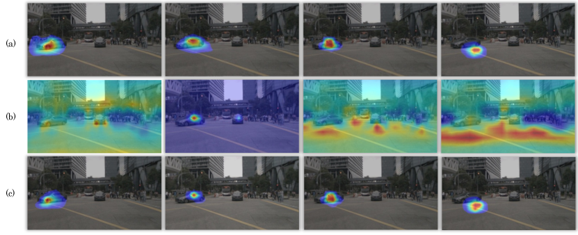
Figure 6: Visualization of attention maps from an object query in the last decoder layer. Four heads out of eight are shown here. We only show a single view for simplicity, (a): the normalized $\mathbf{G}_{n}^{\top}\mathbf{P}_{n}$ (local view attention maps), (b): the normalized $\mathbf{X}_{n}^{\top}\mathbf{O}$ (global view attention maps), (c): the overall attention maps that are the normalized weights of the summation of the former two items. Note that we only visualize the attention weights that are greater than $1e^{-4}$ for better visualization.

Effectiveness of different fusion approaches. The fusion module is used to fuse different frames for temporal modeling. We explore some common fusion approaches for temporal fusion in Tab. 7. We first try a simple fusion approach “concat with MLP”, and achieve $52.7\%$ on NDS, which has $0.5\%$ improvement compared with sharing queries. Considering queries on each frame have similar semantic information and different positional information, we propose the fusion model inspired by the channel attention. As is seen in Tab. 7, our proposed fusion approach “channel att” achieves higher performance compared to simple concatenation operation. We claim that the performance gain is not from the increased parameters since only three fully-connected layers are added in our model. Since queries are defined in each frame’s system and the ego motion occurs between frames, we encode the ego-motion matrix as a high dimensional embedding to align queries in the current frame’s system. With ego-motion embeddings, our fusion approach could further improve $0.6\%$ on NDS and $0.8\%$ on mAP.

4.5 Visualization

We show the visualization of attention maps in Figure  6 from 4 heads out of 8 heads. We display attention maps after the soft-max normalized operation. From the up-bottom way in each row, there are local view attention maps, global view attention maps, and overall attention maps separately. We obverse and draw three conclusions from visualization results. Firstly, local view attention mainly tends to highlight the neighbor of objects, such as the front, middle, and bottom of the objects, while global view attention pays more attention to the whole of images, especially on the ground plane and the same type of objects, as shown in Figure  6 (a). This phenomenon indicates that local view attention and global view attention are complementary to each other. Secondly, as shown in Figure  6 (a) and (c), it can be seen that overall attention maps are highly similar to local view attention maps, which means the local view attention maps play the dominant role compared to global view attention. Thirdly, we could obverse that the overall attention maps are further concentrating on the foreground objects in a fine-grained way, which implies superior localization accuracy.

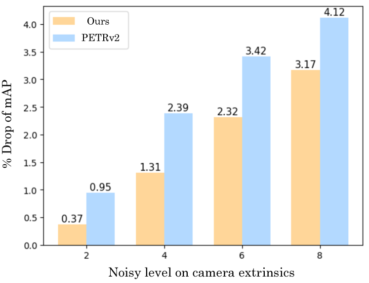
Figure 7: The performance drop of PETRv2 and CAPE-T under different camera extrinsics noise levels on nuScenes validation set.

4.6 Robustness Analysis

We evaluate the robustness of our method on camera extrinsic interference in this section. Camera extrinsic interference is an unavoidable dilemma caused by calibration errors, vehicle jittering, etc. We imitate extrinsics noises on the rotation with different noisy levels following PETRv2 [25] for a fair comparison. Specifically, we randomly sample an angle within the specific range and then multiply the generated noisy rotation matrix by the camera extrinsics in the inference. We present the performance drop of metric mAP on both PETRv2 and CAPE-T in Fig.7. We could see that our method has more robust performances on all noisy levels compared to PETRv2  [25] when facing extrinsics interference. For example, in the noisy level setting $R_{max}=4$, CAPE-T drops 1.31% while PETRv2 drops 2.39%, which shows the superiority of camera-view position embeddings.

5 Conclusion

In this paper, we study the 3D positional embeddings of sparse query-based approaches for multi-view 3D object detection and propose a simple yet effective method CAPE. We form the 3D position embedding under the local camera-view system rather than the global coordinate system, which largely reduces the difficulty of the view transformation learning. Furthermore, we extend our CAPE to temporal modeling by exploiting the fusion between separated queries for temporal frames. It achieves state-of-the-art performance even without LiDAR supervision, and provides a new insight of position embedding in multi-view 3D object detection.

Limitation and future work. The computation and memory cost would be unaffordable when it involves the temporal fusion of long-term frames. In the future, we will dig deeper into more efficient spatial and temporal interaction of 2D and 3D features for autonomous driving systems.

References

- [1] Garrick Brazil and Xiaoming Liu. M3d-rpn: Monocular 3d region proposal network for object detection. In ICCV, pages 9287–9296, 2019.
- [2] Holger Caesar, Varun Bankiti, Alex H Lang, Sourabh Vora, Venice Erin Liong, Qiang Xu, Anush Krishnan, Yu Pan, Giancarlo Baldan, and Oscar Beijbom. nuscenes: A multimodal dataset for autonomous driving. In Proceedings of the IEEE/CVF conference on computer vision and pattern recognition, pages 11621–11631, 2020.
- [3] Nicolas Carion, Francisco Massa, Gabriel Synnaeve, Nicolas Usunier, Alexander Kirillov, and Sergey Zagoruyko. End-to-end object detection with transformers. In ECCV, pages 213–229, 2020.
- [4] Hansheng Chen, Pichao Wang, Fan Wang, Wei Tian, Lu Xiong, and Hao Li. Epro-pnp: Generalized end-to-end probabilistic perspective-n-points for monocular object pose estimation. In CVPR, 2022.
- [5] Qiang Chen, Xiaokang Chen, Gang Zeng, and Jingdong Wang. Group detr: Fast training convergence with decoupled one-to-many label assignment. arXiv preprint arXiv:2207.13085, 2022.
- [6] Shaoyu Chen, Xinggang Wang, Tianheng Cheng, Wenqiang Zhang, Qian Zhang, Chang Huang, and Wenyu Liu. Azinorm: Exploiting the radial symmetry of point cloud for azimuth-normalized 3d perception. In Proceedings of the IEEE/CVF Conference on Computer Vision and Pattern Recognition, pages 6387–6396, 2022.
- [7] Zhiyu Chong, Xinzhu Ma, Hong Zhang, Yuxin Yue, Haojie Li, Zhihui Wang, and Wanli Ouyang. Monodistill: Learning spatial features for monocular 3d object detection. In ICLR, 2021.
- [8] Jiajun Deng, Shaoshuai Shi, Peiwei Li, Wengang Zhou, Yanyong Zhang, and Houqiang Li. Voxel r-cnn: Towards high performance voxel-based 3d object detection. In AAAI, volume 35, pages 1201–1209, 2021.
- [9] Lue Fan, Xuan Xiong, Feng Wang, Naiyan Wang, and Zhaoxiang Zhang. Rangedet: In defense of range view for lidar-based 3d object detection. In Proceedings of the IEEE/CVF International Conference on Computer Vision, pages 2918–2927, 2021.
- [10] Shi Gong, Xiaoqing Ye, Xiao Tan, Jingdong Wang, Errui Ding, Yu Zhou, and Xiang Bai. Gitnet: Geometric prior-based transformation for birds-eye-view segmentation. In ECCV, 2022.
- [11] J. Huang and G. Huang. Bevdet4d: Exploit temporal cues in multi-camera 3d object detection. arXiv e-prints, 2022.
- [12] Junjie Huang, Guan Huang, Zheng Zhu, and Dalong Du. Bevdet: High-performance multi-camera 3d object detection in bird-eye-view. arXiv preprint arXiv:2112.11790, 2021.
- [13] Harold W Kuhn. The hungarian method for the assignment problem. Naval research logistics quarterly, 2(1-2):83–97, 1955.
- [14] Buyu Li, Wanli Ouyang, Lu Sheng, Xingyu Zeng, and Xiaogang Wang. Gs3d: An efficient 3d object detection framework for autonomous driving. In CVPR, pages 1019–1028, 2019.
- [15] Feng Li, Hao Zhang, Shilong Liu, Jian Guo, Lionel M Ni, and Lei Zhang. Dn-detr: Accelerate detr training by introducing query denoising. In CVPR, pages 13619–13627, 2022.
- [16] Peixuan Li, Huaici Zhao, Pengfei Liu, and Feidao Cao. Rtm3d: Real-time monocular 3d detection from object keypoints for autonomous driving. In ECCV, pages 644–660, 2020.
- [17] Yinhao Li, Han Bao, Zheng Ge, Jinrong Yang, Jianjian Sun, and Zeming Li. Bevstereo: Enhancing depth estimation in multi-view 3d object detection with dynamic temporal stereo. arXiv preprint arXiv:2209.10248, 2022.
- [18] Yinhao Li, Zheng Ge, Guanyi Yu, Jinrong Yang, Zengran Wang, Yukang Shi, Jianjian Sun, and Zeming Li. Bevdepth: Acquisition of reliable depth for multi-view 3d object detection. arXiv preprint arXiv:2206.10092, 2022.
- [19] Zhiqi Li, Wenhai Wang, Hongyang Li, Enze Xie, Chonghao Sima, Tong Lu, Qiao Yu, and Jifeng Dai. Bevformer: Learning bird’s-eye-view representation from multi-camera images via spatiotemporal transformers. In ECCV, 2022.
- [20] Qing Lian, Botao Ye, Ruijia Xu, Weilong Yao, and Tong Zhang. Exploring geometric consistency for monocular 3d object detection. In CVPR, pages 1685–1694, 2022.
- [21] Tsung-Yi Lin, Priya Goyal, Ross Girshick, Kaiming He, and Piotr Dollár. Focal loss for dense object detection. In ICCV, pages 2980–2988, 2017.
- [22] Shilong Liu, Feng Li, Hao Zhang, Xiao Yang, Xianbiao Qi, Hang Su, Jun Zhu, and Lei Zhang. Dab-detr: Dynamic anchor boxes are better queries for detr. In ICLR, 2022.
- [23] Xianpeng Liu, Nan Xue, and Tianfu Wu. Learning auxiliary monocular contexts helps monocular 3d object detection. In AAAI, volume 36, pages 1810–1818, 2022.
- [24] Yingfei Liu, Tiancai Wang, Xiangyu Zhang, and Jian Sun. Petr: Position embedding transformation for multi-view 3d object detection. In ECCV, pages 531–548, 2022.
- [25] Yingfei Liu, Junjie Yan, Fan Jia, Shuailin Li, Qi Gao, Tiancai Wang, Xiangyu Zhang, and Jian Sun. Petrv2: A unified framework for 3d perception from multi-camera images. arXiv preprint arXiv:2206.01256, 2022.
- [26] Zhe Liu, Xin Zhao, Tengteng Huang, Ruolan Hu, Yu Zhou, and Xiang Bai. Tanet: Robust 3d object detection from point clouds with triple attention. In AAAI, volume 34, pages 11677–11684, 2020.
- [27] Yan Lu, Xinzhu Ma, Lei Yang, Tianzhu Zhang, Yating Liu, Qi Chu, Junjie Yan, and Wanli Ouyang. Geometry uncertainty projection network for monocular 3d object detection. In ICCV, pages 3111–3121, 2021.
- [28] Depu Meng, Xiaokang Chen, Zejia Fan, Gang Zeng, Houqiang Li, Yuhui Yuan, Lei Sun, and Jingdong Wang. Conditional detr for fast training convergence. In ICCV, pages 3651–3660, 2021.
- [29] Gregory P Meyer, Ankit Laddha, Eric Kee, Carlos Vallespi-Gonzalez, and Carl K Wellington. Lasernet: An efficient probabilistic 3d object detector for autonomous driving. In Proceedings of the IEEE/CVF conference on computer vision and pattern recognition, pages 12677–12686, 2019.
- [30] Arsalan Mousavian, Dragomir Anguelov, John Flynn, and Jana Kosecka. 3d bounding box estimation using deep learning and geometry. In CVPR, pages 7074–7082, 2017.
- [31] Dennis Park, Rares Ambrus, Vitor Guizilini, Jie Li, and Adrien Gaidon. Is pseudo-lidar needed for monocular 3d object detection? In ICCV, pages 3142–3152, 2021.
- [32] Adam Paszke, Sam Gross, Francisco Massa, Adam Lerer, James Bradbury, Gregory Chanan, Trevor Killeen, Zeming Lin, Natalia Gimelshein, Luca Antiga, et al. Pytorch: an imperative style, high-performance deep learning library. In NeurIPS, pages 8026–8037, 2019.
- [33] Jonah Philion and Sanja Fidler. Lift, splat, shoot: Encoding images from arbitrary camera rigs by implicitly unprojecting to 3d. In ECCV, pages 194–210, 2020.
- [34] Charles R Qi, Wei Liu, Chenxia Wu, Hao Su, and Leonidas J Guibas. Frustum pointnets for 3d object detection from rgb-d data. In Proceedings of the IEEE conference on computer vision and pattern recognition, pages 918–927, 2018.
- [35] Rui Qian, Divyansh Garg, Yan Wang, Yurong You, Serge Belongie, Bharath Hariharan, Mark Campbell, Kilian Q Weinberger, and Wei-Lun Chao. End-to-end pseudo-lidar for image-based 3d object detection. In Proceedings of the IEEE/CVF Conference on Computer Vision and Pattern Recognition, pages 5881–5890, 2020.
- [36] Cody Reading, Ali Harakeh, Julia Chae, and Steven L. Waslander. Categorical depth distributionnetwork for monocular 3d object detection. In CVPR, 2021.
- [37] Thomas Roddick and Roberto Cipolla. Predicting semantic map representations from images using pyramid occupancy networks. In CVPR, pages 11138–11147, 2020.
- [38] Thomas Roddick, Alex Kendall, and Roberto Cipolla. Orthographic feature transform for monocular 3d object detection. 2018.
- [39] Shaoshuai Shi, Xiaogang Wang, and Hongsheng Li. Pointrcnn: 3d object proposal generation and detection from point cloud. In CVPR, pages 770–779, 2019.
- [40] Shaoshuai Shi, Zhe Wang, Jianping Shi, Xiaogang Wang, and Hongsheng Li. From points to parts: 3d object detection from point cloud with part-aware and part-aggregation network. IEEE transactions on pattern analysis and machine intelligence, 43(8):2647–2664, 2020.
- [41] Ashish Vaswani, Noam Shazeer, Niki Parmar, Jakob Uszkoreit, Llion Jones, Aidan N Gomez, Łukasz Kaiser, and Illia Polosukhin. Attention is all you need. NeurIPS, 30, 2017.
- [42] Li Wang, Liang Du, Xiaoqing Ye, Yanwei Fu, Guodong Guo, Xiangyang Xue, Jianfeng Feng, and Li Zhang. Depth-conditioned dynamic message propagation for monocular 3d object detection. In CVPR, pages 454–463, 2021.
- [43] Tai Wang, ZHU Xinge, Jiangmiao Pang, and Dahua Lin. Probabilistic and geometric depth: Detecting objects in perspective. In Conference on Robot Learning, pages 1475–1485, 2022.
- [44] Tai Wang, Xinge Zhu, Jiangmiao Pang, and Dahua Lin. Fcos3d: Fully convolutional one-stage monocular 3d object detection. In ICCV, pages 913–922, 2021.
- [45] Yan Wang, Wei-Lun Chao, Divyansh Garg, Bharath Hariharan, Mark Campbell, and Kilian Q Weinberger. Pseudo-lidar from visual depth estimation: Bridging the gap in 3d object detection for autonomous driving. In CVPR, pages 8445–8453, 2019.
- [46] Yue Wang, Vitor Campagnolo Guizilini, Tianyuan Zhang, Yilun Wang, Hang Zhao, and Justin Solomon. Detr3d: 3d object detection from multi-view images via 3d-to-2d queries. In Conference on Robot Learning, pages 180–191, 2022.
- [47] Yingming Wang, Xiangyu Zhang, Tong Yang, and Jian Sun. Anchor detr: Query design for transformer-based detector. In AAAI, volume 36, pages 2567–2575, 2022.
- [48] Junfeng Wu, Yi Jiang, Wenqing Zhang, Xiang Bai, and Song Bai. Seqformer: a frustratingly simple model for video instance segmentation. In ECCV, 2022.
- [49] Xiaoqing Ye, Liang Du, Yifeng Shi, Yingying Li, Xiao Tan, Jianfeng Feng, Errui Ding, and Shilei Wen. Monocular 3d object detection via feature domain adaptation. In ECCV, pages 17–34, 2020.
- [50] Hao Zhang, Feng Li, Shilong Liu, Lei Zhang, Hang Su, Jun Zhu, Lionel Ni, and Harry Shum. Dino: Detr with improved denoising anchor boxes for end-to-end object detection. In International Conference on Learning Representations, 2022.
- [51] Brady Zhou and Philipp Krähenbühl. Cross-view transformers for real-time map-view semantic segmentation. In CVPR, pages 13760–13769, 2022.
- [52] Xizhou Zhu, Weijie Su, Lewei Lu, Bin Li, Xiaogang Wang, and Jifeng Dai. Deformable detr: Deformable transformers for end-to-end object detection. In ICLR, 2021.