A Dynamic Multi-Scale Voxel Flow Network for Video Prediction

Abstract

The performance of video prediction has been greatly boosted by advanced deep neural networks. However, most of the current methods suffer from large model sizes and require extra inputs, e.g., semantic/depth maps, for promising performance. For efficiency consideration, in this paper, we propose a Dynamic Multi-scale Voxel Flow Network (DMVFN) to achieve better video prediction performance at lower computational costs with only RGB images, than previous methods. The core of our DMVFN is a differentiable routing module that can effectively perceive the motion scales of video frames. Once trained, our DMVFN selects adaptive sub-networks for different inputs at the inference stage. Experiments on several benchmarks demonstrate that our DMVFN is an order of magnitude faster than Deep Voxel Flow [35] and surpasses the state-of-the-art iterative-based OPT [63] on generated image quality.

1 Introduction

Video prediction aims to predict future video frames from the current ones. The task potentially benefits the study on representation learning [40] and downstream forecasting tasks such as human motion prediction [39], autonomous driving [6], and climate change [48], etc. During the last decade, video prediction has been increasingly studied in both academia and industry community [7, 5].

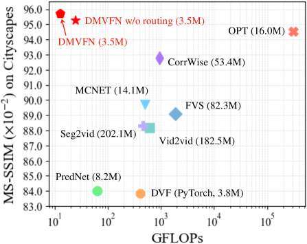
Figure 1: Average MS-SSIM and GFLOPs of different video prediction methods on Cityscapes [9]. The parameter amounts are provided in brackets. DMVFN outperforms previous methods in terms of image quality, parameter amount, and GFLOPs.

Video prediction is challenging because of the diverse and complex motion patterns in the wild, in which accurate motion estimation plays a crucial role [37, 58, 35]. Early methods [37, 58] along this direction mainly utilize recurrent neural networks [19] to capture temporal motion information for video prediction. To achieve robust long-term prediction, the works of [41, 59, 62] additionally exploit the semantic or instance segmentation maps of video frames for semantically coherent motion estimation in complex scenes. However, the semantic or instance maps may not always be available in practical scenarios, which limits the application scope of these video prediction methods [41, 59, 62]. To improve the prediction capability while avoiding extra inputs, the method of OPT [63] utilizes only RGB images to estimate the optical flow of video motions in an optimization manner with impressive performance. However, its inference speed is largely bogged down mainly by the computational costs of pre-trained optical flow model [54] and frame interpolation model [22] used in the iterative generation.

The motions of different objects between two adjacent frames are usually of different scales. This is especially evident in high-resolution videos with meticulous details [49]. The spatial resolution is also of huge differences in real-world video prediction applications. To this end, it is essential yet challenging to develop a single model for multi-scale motion estimation. An early attempt is to extract multi-scale motion cues in different receptive fields by employing the encoder-decoder architecture [35], but in practice it is not flexible enough to deal with complex motions.

In this paper, we propose a Dynamic Multi-scale Voxel Flow Network (DMVFN) to explicitly model the complex motion cues of diverse scales between adjacent video frames by dynamic optical flow estimation. Our DMVFN is consisted of several Multi-scale Voxel Flow Blocks (MVFBs), which are stacked in a sequential manner. On top of MVFBs, a light-weight Routing Module is proposed to adaptively generate a routing vector according to the input frames, and to dynamically select a sub-network for efficient future frame prediction. We conduct experiments on four benchmark datasets, including Cityscapes [9], KITTI [12], DAVIS17 [43], and Vimeo-Test [69], to demonstrate the comprehensive advantages of our DMVFN over representative video prediction methods in terms of visual quality, parameter amount, and computational efficiency measured by floating point operations (FLOPs). A glimpse of comparison results by different methods is provided in Figure 1. One can see that our DMVFN achieves much better performance in terms of accuracy and efficiency on the Cityscapes [9] dataset. Extensive ablation studies validate the effectiveness of the components in our DMVFN for video prediction.

In summary, our contributions are mainly three-fold:

• We design a light-weight DMVFN to accurately predict future frames with only RGB frames as inputs. Our DMVFN is consisted of new MVFB blocks that can model different motion scales in real-world videos.

• We propose an effective Routing Module to dynamically select a suitable sub-network according to the input frames. The proposed Routing Module is end-to-end trained along with our main network DMVFN.

• Experiments on four benchmarks show that our DMVFN achieves state-of-the-art results while being an order of magnitude faster than previous methods.

2 Related Work

2.1 Video Prediction

Early video prediction methods [37, 58, 35] only utilize RGB frames as inputs. For example, PredNet [37] learns an unsupervised neural network, with each layer making local predictions and forwarding deviations from those predictions to subsequent network layers. MCNet [58] decomposes the input frames into motion and content components, which are processed by two separate encoders. DVF [35] is a fully-convolutional encoder-decoder network synthesizing intermediate and future frames by approximating voxel flow for motion estimation. Later, extra information is exploited by video prediction methods in pursuit of better performance. For example, the methods of Vid2vid [59], Seg2vid [41], HVP [32], and SADM [2] require additional semantic maps or human pose information for better video prediction results. Additionally, Qi et al. [44] used extra depth maps and semantic maps to explicitly inference scene dynamics in 3D space. FVS [62] separates the inputs into foreground objects and background areas by semantic and instance maps, and uses a spatial transformer to predict the motion of foreground objects. In this paper, we develop a light-weight and efficient video prediction network that requires only sRGB images as the inputs.

2.2 Optical Flow

Optical flow estimation aims to predict the per-pixel motion between adjacent frames. Deep learning-based optical flow methods [53, 54, 29, 38, 17] have been considerably advanced ever since Flownet [11], a pioneering work to learn optical flow network from synthetic data. Flownet2.0 [25] improves the accuracy of optical flow estimation by stacking sub-networks for iterative refinement. A coarse-to-fine spatial pyramid network is employed in SPynet [46] to estimate optical flow at multiple scales. PWC-Net [53] employs feature warping operation at different resolutions and uses a cost volume layer to refine the estimated flow at each resolution. RAFT [54] is a lightweight recurrent network sharing weights during the iterative learning process. FlowFormer [21] utilizes an encoder to output latent tokens and a recurrent decoder to decode features, while refining the estimated flow iteratively. In video synthesis, optical flow for downstream tasks [69, 35, 22, 68, 72] is also a hot research topic. Based on these approaches, we aim to design a flow estimation network that can adaptively operate based on each sample for the video prediction task.

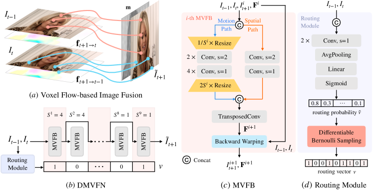
Figure 2: Overview of the proposed Dynamic Multi-scale Voxel Flow Network (DMVFN). $(a)$: To predict a future frame, we use the voxel flow [35] to guide the pixel fusion of the input frames. The voxel flow contains the prediction of object motion and occlusion. $(b)$: DMVFN contains several MVFBs with decreasing scaling factor $S^{i}$. According to the routing vector $v$ estimated by a Routing Module, a sub-network is selected to process the input image. $(c)$: Each MVFB has a scaling factor $S^{i}$, which means that the motion path is performed on images whose sizes are $1/S^{i}$ of the original. $(d)$: Two consecutive frames are fed into several neural layers and a Differentiable Bernoulli sample to generate the hard routing vector.

2.3 Dynamic Network

The design of dynamic networks is mainly divided into three categories: spatial-wise, temporal-wise, and sample-wise [16]. Spatial-wise dynamic networks perform adaptive operations in different spatial regions to reduce computational redundancy with comparable performance [47, 57, 20]. In addition to the spatial dimension, dynamic processing can also be applied in the temporal dimension. Temporal-wise dynamic networks [70, 52, 64] improve the inference efficiency by performing less or no computation on unimportant sequence frames. To handle the input in a data-driven manner, sample-wise dynamic networks adaptively adjust network structures to side-off the extra computation [60, 56], or adaptively change the network parameters to improve the performance [18, 51, 10, 76]. Designing and training a dynamic network is not trivial since it is difficult to directly enable a model with complex topology connections. We need to design a well-structured and robust model before considering its dynamic mechanism. In this paper, we propose a module to dynamically perceive the motion magnitude of input frames to select the network structure.

3 Methodology

3.1 Background

Video prediction.

Given a sequence of past $t$ frames $\{I_{i}\in\mathbb{R}^{h\times w\times 3}|i=1,...,t\}$, video prediction aims to predict the future frames $\{\tilde{I}_{t+1},\tilde{I}_{t+2},\tilde{I}_{t+3},\ ...\}$. The inputs of our video prediction model are only the two consecutive frames $I_{t-1}$ and $I_{t}$. We concentrate on predicting $\tilde{I}_{t+1}$, and iteratively predict future frames $\{\tilde{I}_{t+2},\tilde{I}_{t+3},\ ...\}$ in a similar manner. Denote the video prediction model as $G_{\theta}(I_{t-1},I_{t})$, where $\theta$ is the set of model parameters to be learned, the learning objective is to minimize the difference between $\tilde{I}_{t+1}=G_{\theta}(I_{t-1},I_{t})$ and the “ground truth” $I_{t+1}$.

Voxel flow.

Considering the local consistency in space-time, the pixels of a generated future frame come from nearby regions of the previous frames [75, 69]. In video prediction task, researchers estimate optical flow $\textbf{f}_{t+1\rightarrow t}$ from $I_{t+1}$ to $I_{t}$ [35]. And the corresponding frame is obtained using the pixel-wise backward warping [26] (denoted as $\overleftarrow{\mathcal{W}}$). In addition, to deal with the occlusion, some methods [28, 35] further introduce a fusion map m to fuse the pixels of $I_{t}$ and $I_{t-1}$. The final predicted frame is obtained by the following formulation (Figure 2 $(a)$):

$$\hat{I}_{t+1\leftarrow{t-1}}=\overleftarrow{\mathcal{W}}(I_{t-1},\textbf{f}_{t+1\rightarrow t-1}),$$ (1)

$$\hat{I}_{t+1\leftarrow{t}}=\overleftarrow{\mathcal{W}}(I_{t},\textbf{f}_{t+1\rightarrow t}),$$ (2)

$$\tilde{I}_{t+1}=\hat{I}_{t+1\leftarrow{t-1}}\times\textbf{m}+\hat{I}_{t+1\leftarrow{t}}\times(1-\textbf{m}).$$ (3)

Here, $\hat{I}_{t+1\leftarrow{t}}$ and $\hat{I}_{t+1\leftarrow{t-1}}$ are intermediate warped images. To simplify notations, we refer to the optical flows $\textbf{f}_{t+1\rightarrow t},\textbf{f}_{t+1\rightarrow t-1}$ and the fusion map m collectively as the voxel flow $\textbf{F}_{t+1}$, similar to the notations in [35]. The above equations can be simplified to the following form:

$$\tilde{I}_{t+1}=\overleftarrow{\mathcal{W}}(I_{t-1},I_{t},\textbf{F}_{t+1}).$$ (4)

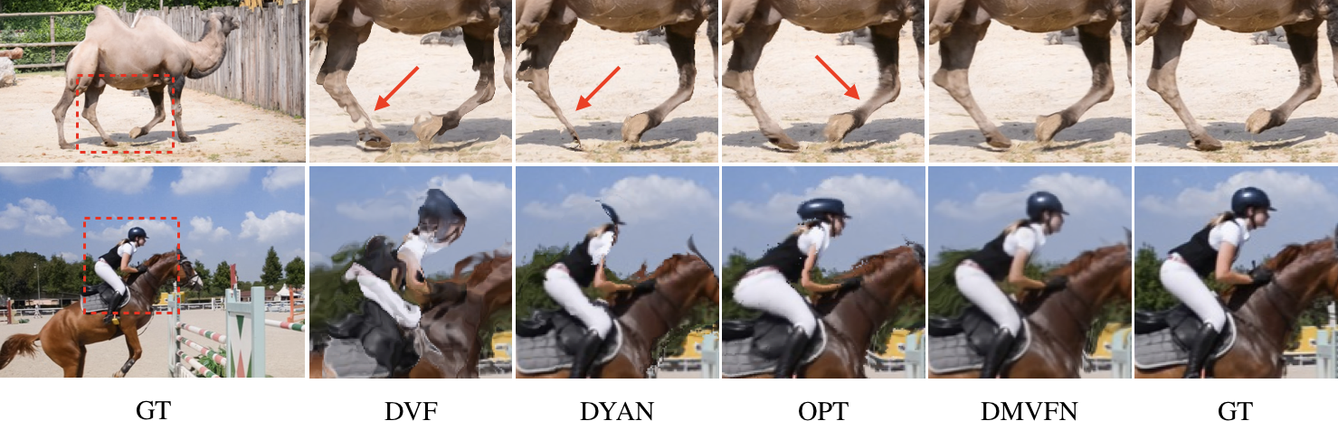
Figure 3: Visual comparison of ($t+1$)-th frame predicted from $t$-th and ($t-1$)-th frames on the DAVIS17-Val [43].

3.2 Dynamic Multi-Scale Voxel Flow Network

MVFB.

To estimate the voxel flow, DVF [35] assumes that all optical flows are locally linear and temporally symmetric around the targeted time, which may be unreasonable for large-scale motions. To address the object position changing issue [22] in adjacent frames, OPT [63] uses flow reversal layer [68] to convert forward flows to backward flows. We aim to estimate voxel flow end-to-end without introducing new components and unreasonable constraints.

We denote the $i$-th MVFB as $f^{i}_{MVFB}(\cdot)$. It learns to approximate target voxel flow $\textbf{F}^{i}_{t+1}$ by taking two frames $I_{t-1}$ and $I_{t}$, the synthesized frame $\tilde{I}^{i-1}_{t+1}$, and the voxel flow estimated by previous blocks $\textbf{F}^{i-1}_{t+1}$ as inputs.

The architecture of our MVFB is shown in Figure 2 $(c)$. To capture the large motion while retaining the original spatial information, we construct a two-branch network structure [71]. This design inherits from pyramidal optical flow estimation [53, 46]. In the motion path, the input is down-sampled by a scaling factor $S^{i}$ to facilitate the expansion of the receptive field. Another spatial path operates at high resolution to complement the spatial information. We denote $\tilde{I}^{i}_{t+1}$ as the output of the $i$-th MVFB. Formally,

$$\tilde{I}^{i}_{t+1},\textbf{F}^{i}_{t+1}=f_{\mathrm{MVFB}}^{i}(I_{t-1},I_{t},\tilde{I}^{i-1}_{t+1},\textbf{F}^{i-1}_{t+1},S^{i}).$$ (5)

The initial values of $\tilde{I}_{t+1}^{0}$ and $\textbf{F}^{0}_{t+1}$ are set to zero. As illustrated in Figure 2 $(b)$, our DMVFN contains $9$ MVFBs. To generate a future frame, we iteratively refine a voxel flow [35] and fuse the pixels of the input frames.

Many optical flow estimation methods predict the flow field on a small image, and then refine it on a large image [53, 67]. For simplicity and intuition, we consider decreasing scaling factor sequences. Finally, the scaling factors is experimentally set as $[4,4,4,2,2,2,1,1,1]$.

DMVFN.

Different pairs of adjacent frames have diverse motion scales and different computational demands. An intuitive idea is to adaptively select dynamic architectures conditioned on each input. We then perform dynamic routing within the super network (the whole architecture) [16], including multiple possible paths. DMVFN saves redundant computation for samples with small-scale motion and preserves the representation ability for large-scale motion.

To make our DMVFN end-to-end trainable, we design a differentiable Routing Module containing a tiny neural network to estimate routing vector $v$ for each input sample. Based on this vector, our DMVFN dynamically selects a sub-network to process the input data. As the figure shows, some blocks are skipped during inference.

Different from some dynamic network methods that can only continuously select the first several blocks ($n$ options) [55, 4], DMVFN is able to choose paths freely ($2^{n}$ options). DMVFN trains different sub-networks in the super network with various possible inference paths and uses dynamic routing inside the super network during inference to reduce redundant computation while maintaining the performance. A dynamic routing vector $v\in{\{0,1\}}^{n}$ is predicted by the proposed Routing Module. For the $i$-th MVFN block of DMVFN, we denote $v_{i}$ as the reference of whether processing the reached voxel flow $\textbf{F}^{i-1}_{t+1}$ and the reached predicted frame $\tilde{I}^{i-1}_{t+1}$. The path $f^{i}_{\mathrm{MVFB}}$ to the $i$-th block from the last block will be activated only when $v_{i}=1$. Formally,

$$\tilde{I}^{i}_{t+1},\textbf{F}^{i}_{t+1}=\begin{cases}f^{i}_{\mathrm{MVFB}}(\tilde{I}^{i-1}_{t+1},\textbf{F}^{i-1}_{t+1}),&v_{i}=1\\ \\ \tilde{I}^{i-1}_{t+1},\textbf{F}^{i-1}_{t+1},&v_{i}=0.\end{cases}$$ (6)

During the training phase, to enable the backpropagation of Eqn. (6), we use $v_{i}$ and $(1-v_{i})$ as the weights of the two branches and average their outputs.

Table 1: Quantitative results of different methods on the Cityscapes [9], and KITTI [12] datasets. “RGB”, “F”, “S” and “I” denote the video frames, optical flow, semantic map, and instance map, respectively. We denote our DMVFN without routing module as “DMVFN (w/o r)”. FVS [62] integrates a segmentation model [77] on KITTI [12] to obtain the semantic maps. “N/A” means not available.

Method	Inputs	Cityscapes-Train$\rightarrow$Cityscapes-Test [9]							KITTI-Train$\rightarrow$KITTI-Test [12]
		GFLOPs	MS-SSIM ($\times 10^{-2}$) $\uparrow$			LPIPS ($\times 10^{-2}$) $\downarrow$			GFLOPs	MS-SSIM ($\times 10^{-2}$) $\uparrow$			LPIPS ($\times 10^{-2}$) $\downarrow$
			$t+1$	$t+3$	$t+5$	$t+1$	$t+3$	$t+5$		$t+1$	$t+3$	$t+5$	$t+1$	$t+3$	$t+5$
Vid2vid [59]	RGB+S	603.79	88.16	80.55	75.13	10.58	15.92	20.14	N/A	N/A	N/A	N/A	N/A	N/A	N/A
Seg2vid [41]	RGB+S	455.84	88.32	N/A	61.63	9.69	N/A	25.99	N/A	N/A	N/A	N/A	N/A	N/A	N/A
FVS [62]	RGB+S+I	1891.65	89.10	81.13	75.68	8.50	12.98	16.50	768.96	79.28	67.65	60.77	18.48	24.61	30.49
SADM [2]	RGB+S+F	N/A	95.99	N/A	83.51	7.67	N/A	14.93	N/A	83.06	72.44	64.72	14.41	24.58	31.16
PredNet [37]	RGB	62.62	84.03	79.25	75.21	25.99	29.99	36.03	25.44	56.26	51.47	47.56	55.35	58.66	62.95
MCNET [58]	RGB	502.80	89.69	78.07	70.58	18.88	31.34	37.34	204.26	75.35	63.52	55.48	24.05	31.71	37.39
DVF [35]	RGB	409.78	83.85	76.23	71.11	17.37	24.05	28.79	166.47	53.93	46.99	42.62	32.47	37.43	41.59
CorrWise [13]	RGB	944.29	92.80	N/A	83.90	8.50	N/A	15.00	383.62	82.00	N/A	66.70	17.20	N/A	25.90
OPT [63]	RGB	313482.15	94.54	86.89	80.40	6.46	12.50	17.83	127431.71	82.71	69.50	61.09	12.34	20.29	26.35
DMVFN (w/o r)	RGB	24.51	95.29	87.91	81.48	5.60	10.48	14.91	9.96	88.06	76.53	68.29	10.70	19.28	26.13
DMVFN	RGB	12.71	95.73	89.24	83.45	5.58	10.47	14.82	5.15	88.53	78.01	70.52	10.74	19.27	26.05

In the iterative scheme of our DMVFN, each MVFB essentially refines the current voxel flow estimation to a new one. This special property allows our DMVFN to skip some MVFBs for every pair of input frames. Here, we design a differentiable and efficient routing module for learning to trade-off each MVFB block. This is achieved by predicting a routing vector $v\in\{0,1\}^{n}$ to identify the proper sub-network (e.g., 0 for deactivated MVFBs, 1 for activated MVFBs). We implement the routing module by a small neural network ($\sim 1/6$ GFLOPs of the super network), and show its architecture in Figure 2 $(d)$. It learns to predict the probability $\tilde{v}$ of choosing MVFBs by:

$$\tilde{v}=\text{Linear}(\text{AvgPooling}(\text{Convs}(I_{t-1},I_{t}))),$$ (7)

$$v=\text{Bernoulli-Sampling}(\tilde{v}).$$ (8)

Differentiable Routing.

To train the proposed Routing Module, we need to constrain the probability values to prevent the model from falling into trivial solutions (e.g., select all blocks). On the other hand, we allow this module to participate in the gradient calculation to achieve end-to-end training. We introduce the Gumbel Softmax [27] and the Straight-Through Estimator (STE) [3] to tackle this issue.

One popular method to make the routing probability $\tilde{v}$ learnable is the Gumbel Softmax technique [27, 24]. By treating the selection of each MVFB as a binary classification task, the soft dynamic routing vector $v\in\mathbb{R}^{n}$ is

$$v_{i}=\frac{\exp\big{(}\frac{1}{\tau}(\tilde{v}_{i}+G_{i})\big{)}}{\exp\big{(}\frac{1}{\tau}(\tilde{v}_{i}+G_{i})\big{)}+\exp\big{(}\frac{1}{\tau}(2-\tilde{v}_{i}-G_{i})\big{)}},$$ (9)

where $i=1,...,n$, $G_{i}\in\mathbb{R}$ is Gumbel noise following the Gumbel$(0,1)$ distribution, and $\tau$ is a temperature parameter. We start at a very high temperature to ensure that all possible paths become candidates, and then the temperature is attenuated to a small value to approximate one-hot distribution. To encourage the sum of the routing vectors $\{v_{i}\}_{i=1}^{n}$ to be small, we add the regularization term ($\frac{1}{n}\sum^{n}_{i=1}v_{i}$) to the final loss function. However, we experimentally find that our DMVFN usually converges to an input-independent structure when temperature decreases. We conjecture that the control of the temperature parameter $\tau$ and the design of the regularization term require further study.

Inspired by previous research on low-bit width neural networks [74, 23], we adopt STE for Bernoulli Sampling (STEBS) to make the binary dynamic routing vector differentiable. An STE can be regarded as an operator that has arbitrary forward and backward operations. Formally,

$$\tilde{w}_{i}=\min(\beta\times n\times\sigma(\tilde{v}_{i})/\sum_{i}^{n}\sigma(\tilde{v}_{i}),1),$$ (10)

$$\textbf{STE Forward}:v_{i}\sim\text{Bernoulli}(\tilde{w}_{i}),$$ (11)

$$\textbf{STE Backward}:\frac{\partial o}{\partial\tilde{w}}=\frac{\partial o}{\partial v},$$ (12)

where $\sigma$ is the Sigmoid function and we denote the objective function as $o$. We use the well-defined gradient $\frac{\partial o}{\partial v}$ as an approximation for $\frac{\partial o}{\partial\tilde{w}}$ to construct the backward pass. In Eqn. (10), we normalize the sample rate. During training, $\beta$ is fixed at $0.5$. We can adjust the hyper-parameter $\beta$ to control the complexity in the inference phase.

Table 2: Quantitative results on the DAVIS17-Val [43] and Vimeo90K-Test [69] benchmarks. We denote DMVFN without routing as “DMVFN (w/o r)”. “N/A” means not available.

Method	UCF101-Train$\rightarrow$DAVIS17-Val					UCF101-Train$\rightarrow$Vimeo90K-Test
	GFLOPs $\downarrow$	MS-SSIM ($\times 10^{-2}$) $\uparrow$		LPIPS ($\times 10^{-2}$) $\downarrow$		GFLOPs $\downarrow$	MS-SSIM ($\times 10^{-2}$) $\uparrow$	LPIPS ($\times 10^{-2}$) $\downarrow$
		$t+1$	$t+3$	$t+1$	$t+3$		$t+1$	$t+1$
DVF [35]	324.15	68.61	55.47	23.23	34.22	89.64	92.11	7.73
DYAN [34]	130.12	78.96	70.41	13.09	21.43	N/A	N/A	N/A
OPT [63]	165312.80	83.26	73.85	11.40	18.21	45716.20	96.75	3.59
DMVFN (w/o r)	19.39	84.81	75.05	9.41	16.24	5.36	97.24	3.30
DMVFN	9.96	83.97	74.81	9.96	17.28	2.77	97.01	3.69

3.3 Implementation Details

Loss function. Our training loss ${L}_{total}$ is the sum of the reconstruction losses of outputs of each block ${I}^{i}_{t+1}$:

$${L}_{total}=\sum_{i=1}^{n}\gamma^{n-i}d(\tilde{I}^{i}_{t+1},I_{t+1}),$$ (13)

where $d$ is the $\ell_{1}$ loss calculated on the Laplacian pyramid representations [42] extracted from each pair of images. And we set $\gamma=0.8$ in our experiments following [54].

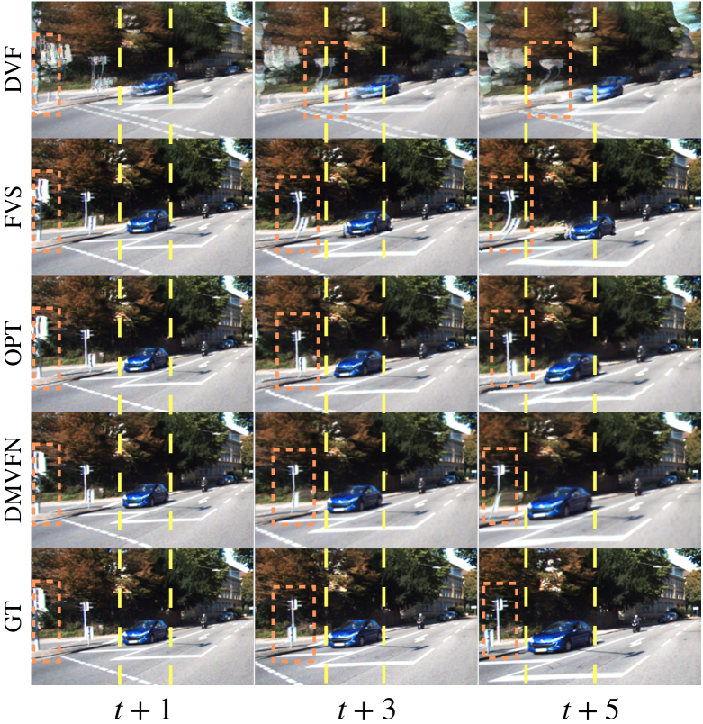
Figure 4: Prediction comparison on KITTI. The yellow line is aligned with the car in the ground truth. The results show that previous methods (DVF [35], FVS [62], and OPT [63]) cannot accurately predict the car’s location in the long-term prediction. The motion predicted by our DMVFN is the most similar to the ground truth, while the errors of other methods grow larger with time. The fences predicted by DMVFN remain vertical when moving.

Training strategy.

Our DMVFN is trained on $224\times 224$ image patches. The batch size is set as $64$. We employ the AdamW optimizer [30, 36] with a weight decay of $10^{-4}$. We use a cosine annealing strategy to reduce the learning rate from $10^{-4}$ to $10^{-5}$. Our model is trained on four 2080Ti GPUs for $300$ epochs, which takes about $35$ hours.

4 Experiments

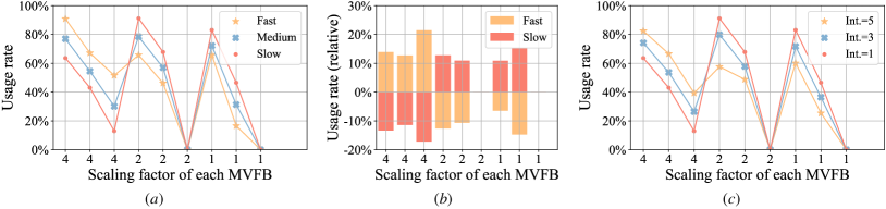
Figure 5: $(a)$: Average usage rate on videos with different motion magnitudes. “Fast”: tested on Vimeo-Fast. “Medium”: tested on Vimeo-Medium. “Slow”: tested on Vimeo-Slow. $(b)$: Difference between “Fast”/“Slow” and “Medium” of $(a)$. $(c)$: Averaged usage rate on different time intervals between two input frames from Vimeo-Slow. “Int.”: time interval.

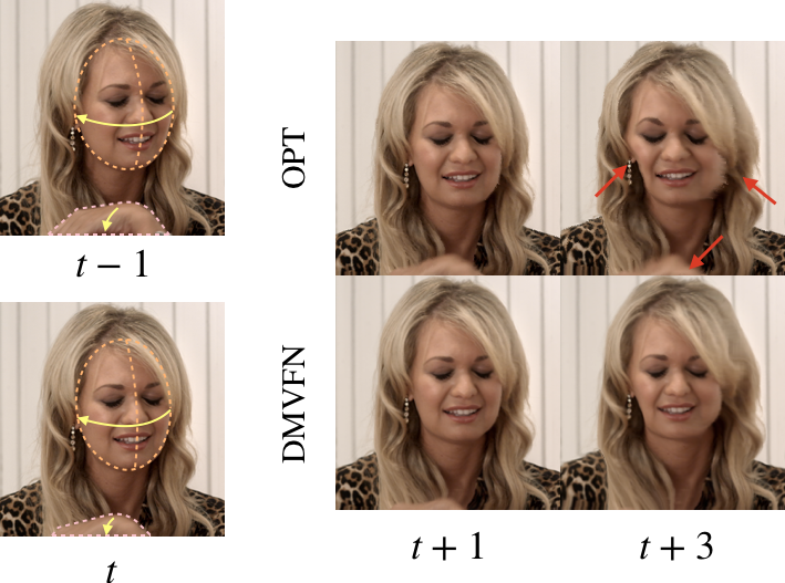
Figure 6: Visual effect comparison in the Vimeo-Test [69] dataset. our DMVFN faithfully reproduces the motion of the hand and the head with less distortion and artifacts.

4.1 Dataset and Metric

Dataset.

We use several datasets in the experiments:

Cityscapes dataset [9] contains 3,475 driving videos with resolution of $2048\times 1024$. We use 2,945 videos for training (Cityscapes-Train) and 500 videos in Cityscapes dataset [9] for testing (Cityscapes-Test).

KITTI dataset [12] contains 28 driving videos with resolution of $375\times 1242$. 24 videos in KITTI dataset are used for training (KITTI-Train) and the remaining four videos in KITTI dataset are used for testing (KITTI-Test).

UCF101 [50] dataset contains $13,320$ videos under 101 different action categories with resolution of $240\times 320$. We only use the training subset of UCF101 [50].

Vimeo90K [69] dataset has $51,312$ triplets for training, where each triplet contains three consecutive video frames with resolution of $256\times 448$. There are $3,782$ triplets in the Vimeo90K testing set. We denote the training and testing subsets as Vimeo-Train and Vimeo-Test, respectively.

DAVIS17 [43] has videos with resolution around $854\times 480$. We use the DAVIS17-Val containing 30 videos as test set.

Configurations. We have four experimental configurations following previous works [34, 35, 63]:

• Cityscapes-Train$\rightarrow$Cityscapes-Test

• KITTI-Train$\rightarrow$KITTI-Test

• UCF101$\rightarrow$DAVIS17-Val

• UCF101$\rightarrow$Vimeo-Test

Here, the left and right sides of the arrow represent the training set and the test set, respectively. For a fair comparison with other methods that are not tailored for high resolution videos, we follow the setting in [62] and resize the images in Cityscapes [9] to $1024\times 512$ and images in KITTI [12] to $256\times 832$, respectively. During inference of Cityscapes [9] and KITTI [12], we predict the next five frames. We predict the next three frames for DAVIS17-Val [43] and next one frame for Vimeo-Test [69], respectively. Note that OPT [63] is an optimization-based approach and uses pre-trained RAFT [54] and RIFE [22] models. RIFE [22] and RAFT [54] are trained on the Vimeo-Train dataset [69] and the Flying Chairs dataset [11], respectively.

Evaluation metrics. Following previous works [63], we use Multi-Scale Structural Similarity Index Measure (MS-SSIM) [61] and a perceptual metric LPIPS [73] for quantitative evaluation. To measure the model complexity, we calculate the GFLOPs.

4.2 Comparison to State-of-the-Arts

We compare our DMVFN with state-of-the-art video prediction methods. These methods fall into two categories: the methods requiring only RGB images as input (e.g., PredNet [37], MCNET [58], DVF [35], CorrWise [13], OPT [63]) and the methods requiring extra information as input (e.g., Vid2vid [59], Seg2vid [41], FVS [62], SADM [2]).

Quantitative results. The quantitative results are reported in Table 1 and Table 2. When calculating the GFLOPs of OPT [63], the number of iterations is set as $3,000$. In terms of MS-SSIM and LPIPS, our DMVFN achieves much better results than the other methods in both short-term and long-term video prediction tasks. The GFLOPs of our DMVFN is considerably smaller than the comparison methods. These results show the proposed routing strategy reduces almost half the number of GFLOPs while maintaining comparable performance. Because the decrease of GFLOPs is not strictly linear with the actual latency [45], we measure the running speed on TITAN 2080Ti. For predicting a 720P frame, DVF [35] spends $0.130$s on average, while our DMVFN only needs $0.023$s on average.

Table 3: Comparison between DMVFN and STRPM.

Method	UCF Sports		Human3.6M
	$t+1$	$t+6$	$t+1$	$t+4$
	PSNR$\uparrow$ / LPIPS$\downarrow$	PSNR$\uparrow$ / LPIPS$\downarrow$	PSNR$\uparrow$ / LPIPS$\downarrow$	PSNR$\uparrow$ / LPIPS$\downarrow$
STRPM	28.54 / 20.69	20.59 / 41.11	33.32 / 9.74	29.01 / 10.44
DMVFN	30.05 / 10.24	22.67 / 22.50	35.07 / 7.48	29.56 / 9.74

More comparison. The quantitative results compared with STRPM [8] are reported in Table 3. We train our DMVFN in UCFSports and Human3.6M datasets following the setting in [8]. We also measure the average running speed on TITAN 2080Ti. To predict a $1024\times 1024$ frame, our DMVFN is averagely 4.06$\times$ faster than STRPM [8].

Qualitative results on different datasets are shown in Figure 3, Figure 4 and Figure 6. As we can see, the frames predicted by our DMVFN exhibit better temporal continuity and are more consistent with the ground truth than those by the other methods. Our DMVFN is able to predict correct motion while preserving the shape and texture of objects.

4.3 Ablation Study

Here, we perform extensive ablation studies to further study the effectiveness of components in our DMVFN. The experiments are performed on the Cityscapes [9] and KITTI [12] datasets unless otherwise specified.

1) How effective is the proposed Routing Module? As suggested in [65, 66], we divide the Vimeo-90K [69] test set into three subsets: Vimeo-Fast, Vimeo-Medium, and Vimeo-Slow, which correspond to the motion range. To verify that our DMVFN can perceive motion scales and adaptively choose the proper sub-networks, we retrain our DMVFN on the Vimeo-Train [69] using the same training strategy in §3.3. We calculate the averaged usage rate of each MVFB on three test subsets. From Figures 5 $(a)$ and 5 $(b)$, we observe that our DMVFN prefers to select MVFBs with large scale (e.g., 4x) for two frames with large motion. There are two MVFBs with clearly smaller selection probability. We believe this reflects the inductive bias of our DMVFN on different combinations of scaling factors.

To further verify that our DMVFN also perceives the size of the time interval, we test our DMVFN on the two frames with different time intervals (but still in the same video). We choose Vimeo-Slow as the test set, and set the time intervals as $1$, $3$, and $5$. The results are shown in Figure 5 $(c)$. We observe that our DMVFN prefers large-scale blocks on long-interval inputs, and small-scale blocks on short-interval inputs. This verifies that our DMVFN can perceive temporal information and dynamically select different sub-networks to handle the input frames with different time intervals.

To further study how the MVFBs are selected, we select 103 video sequences (contain a high-speed moving car and a relatively static background) from the KITTI dataset, denoted as KITTI-A. As shown in Table 4, on the KITTI-A dataset, our DMVFN prefers to choose MVFBs with large scaling factors to capture large movements. The flow estimation for static backgrounds is straightforward, while the large motion dominates the choice of our DMVFN.

Table 4: Average usage rate ($10^{-2}$) of MVFBs in our DMVFN.

Scale	$4$	$4$	$4$	$2$	$2$	$2$	$1$	$1$	$1$
KITTI-A	$80.95$	$34.22$	$26.70$	$81.19$	$73.91$	$44.90$	$55.34$	$0.49$	$0$

Table 5: Routing Module based on STEBS is effective. The evaluation metric is MS-SSIM ($\times 10^{-2}$).

Setting	Cityscapes			KITTI
	$t+1$	$t+3$	$t+5$	$t+1$	$t+3$	$t+5$
Copy last frame	76.95	68.82	64.45	58.31	48.99	44.16
w/o routing	95.29	87.91	81.48	88.06	76.53	68.29
Random	91.97	82.11	70.05	81.31	69.89	62.42
Gumbel Softmax	95.05	87.57	79.54	87.42	75.56	65.83
STEBS	95.73	89.24	83.45	88.53	78.01	70.52

2) How to design the Routing Module? A trivial solution is to process the routing probability $p$ with Gumbel Softmax. The comparison results of our DMVFNs with different differentiable routing methods are summarized in Table 5. Our DMVFN with STEBS outperforms the DMVFN variant with Gumbel Softmax on MS-SSIM, especially for long-term prediction. The DMVFN variant with Gumbel Softmax usually degenerates to a fixed and static structure. We also compare with the DMVFN randomly selecting each MVFB with probability $0.5$ (denoted as “Random”) and that without routing module (denoted as “w/o routing”).

Table 6: Results of our DMVFN with different scaling factor settings. The evaluation metric is MS-SSIM ($\times 10^{-2}$).

Setting	Cityscapes			KITTI
in DMVFN	$t+1$	$t+3$	$t+5$	$t+1$	$t+3$	$t+5$
$[1]$	94.70	87.26	80.93	87.64	76.71	68.76
$[2,1]$	95.30	87.93	82.02	87.97	77.23	69.58
$[4,2,1]$	95.73	89.24	83.45	88.53	78.01	70.52

3) How to set the scaling factors? We evaluate our DMVFN with different scaling factors. We use three non-increasing factor sequences of “$[1,1,1,1,1,1,1,1,1]$”, “$[2,2,2,2,2,1,1,1,1]$” and “$[4,4,4,2,2,2,1,1,1]$”, denoted as “$[1]$”, “$[2,1]$” and “$[4,2,1]$”, respectively. The results are listed in Table 6. Our DMVFN with “$[4,2,1]$” performs better than that with “$[2,1]$” and “$[1]$”. The gap is more obvious on longer-term future frames.

Table 7: Spatial path is effective in our DMVFN. The evaluation metric is MS-SSIM ($\times 10^{-2}$).

Setting	Cityscapes			KITTI
	$t+1$	$t+3$	$t+5$	$t+1$	$t+3$	$t+5$
w/o r, w/o path	94.99	87.59	80.98	87.75	76.22	67.86
w/o r	95.29	87.91	81.48	88.06	76.53	68.29
w/o path	95.55	88.89	83.03	88.29	77.53	69.86
DMVFN	95.73	89.24	83.45	88.53	78.01	70.52

4) How effective is the spatial path? To verify the effectiveness of the spatial path in our DMVFN, we compare it with the DMVFN without spatial path (denoted as “w/o path”). The results listed in Table 7 show our DMVFN enjoys better performance with the spatial path, no matter with or without the routing module (denoted as “w/o r”).

5 Conclusion

In this work, we developed an efficient Dynamic Multi-scale Voxel Flow Network (DMVFN) that excels previous video prediction methods on dealing with complex motions of different scales. With the proposed routing module, our DMVFN adaptively activates different sub-networks based on the input frames, improving the prediction performance while reducing the computation costs. Experiments on diverse benchmark datasets demonstrated that our DMVFN achieves state-of-the-artperformance with greatly reduced computation burden. We believe our DMVFN can provide general insights for long-term prediction, video frame synthesis, and representation learning [15, 14]. We hope our DMVFN will inspire further research in light-weight video processing and make video prediction more accessible for downstream tasks such as CODEC for streaming video.

Our DMVFN can be improved at several aspects. Firstly, iteratively predicting future frames suffers from accumulate errors. This issue may be addressed by further bringing explicit temporal modeling [68, 66, 31, 22] to our DMVFN. Secondly, our DMVFN simply selects the nodes in a chain network topology, which can be improved by exploring more complex topology. For example, our routing module can be extended to automatically determine the scaling factors for parallel branches [33]. Thirdly, forecast uncertainty modeling is more of an extrapolation abiding to past flow information, especially considering bifurcation, which exceeds the current capability of our DMVFN. We believe that research on long-term forecast uncertainty may uncover deeper interplay with dynamic modeling methods [14, 1].

Acknowledgements. We sincerely thank Wen Heng for his exploration on neural architecture search at Megvii Research and Tianyuan Zhang for meaningful suggestions. This work is supported in part by the National Natural Science Foundation of China (No. 62002176 and 62176068).

Supplemental File to “A Dynamic Multi-Scale Voxel Flow Network for Video Prediction”

We provide more details of DMVFN for video prediction. Specifically, we provide

• societal impact in §6.

• visualization of voxel flow §7;

• more ablation studies in §8;

6 Societal Impact

This work potentially benefits video prediction and dynamic neural network fields. The authors believe that this work has small potential negative impacts.

7 Visualization of Voxel Flow

We visualize the voxel flow predicted by DMVFN in Figure 7. We use the optical flow generated by RAFT [54] as a reference. We observe that the optical flow $\textbf{f}_{t+1\rightarrow t}$ and the map $1-\textbf{m}$ of most pixels are successfully predicted by DMVFN. This demonstrates that our DMVFN can indeed accurately predict a voxel flow.

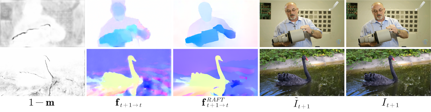
Figure 7: Visualization of the map $1-\textbf{m}$, the optical flow $\textbf{f}_{t+1\rightarrow t}$, the optical flow by RAFT [54] $\textbf{f}^{RAFT}_{t+1\rightarrow t}$, the predicted frame $\tilde{I}_{t+1}$ and the “ground truth” $I_{t+1}$.

8 More Ablation Study Results

5) How does $\beta$ influence the performance of DMVFN during inference? The $\beta$ is an important factor to control the model complexity and prediction capability during inference. Here, we adjust $\beta$ during the inference phase, as shown in Table 8. DMVFN with larger $\beta$ enjoys better MS-SSIM results but suffers from higher complexity.

Table 8: Results of DMVFN with different $\beta$ evaluated on KITTI benchmark [12].

Settings ($\beta=$)	$0.3$	$0.4$	$0.5$	$0.6$	$0.7$	$0.8$
GFLOPs	2.62	3.88	5.15	5.94	6.21	6.40
LPIPS	16.47	12.91	10.74	10.26	10.24	10.23
MS-SSIM ($\times 10^{-2}$)	78.78	85.13	88.53	88.89	88.89	88.89

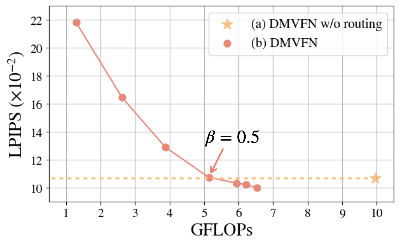
Figure 8: Control the complexity of DMVFN by adjusting $\beta$. DMVFN saves half GFLOPs of comparable performance compared to DMVFN without routing.

6) How to design the loss function? To study this problem, we train our DMVFN and DMVFN (w/o routing) only optimizing the loss on output of the last block $\tilde{I}_{t+1}$ (denoted as “single supervision”). The results listed in Table 9 show the advantages of our loss function $L_{total}$. $L_{total}$ is calculated on all intermediate results of DMVFN.

Table 9: Results of DMVFN with different loss settings. The evaluation metric is MS-SSIM ($\times 10^{-2}$).

Settings	Cityscapes			KITTI			Davis17-Val		Vimeo-Test
	t+1	t+3	t+5	t+1	t+3	t+5	t+1	t+3	t+1
w/o routing, single supervision	95.19	87.77	81.22	87.91	76.33	67.99	84.69	74.92	97.18
w/o routing	95.29	87.91	81.48	88.06	76.53	68.29	84.81	75.05	97.24
single supervision	95.65	89.10	83.27	88.34	77.88	70.18	83.83	74.68	96.95
DMVFN	95.73	89.24	83.45	88.53	78.01	70.52	83.97	74.81	97.01

Table 10: Routing Module based on STEBS is effective. The evaluation metric is MS-SSIM ($\times 10^{-2}$).

Settings	Cityscapes			KITTI			Davis-Val		Vimeo-Test
	t+1	t+3	t+5	t+1	t+3	t+5	t+1	t+3	t+1
w/o routing	95.29	87.91	81.48	88.06	76.53	68.29	84.81	75.05	97.24
Random	91.97	82.11	70.05	81.31	69.89	62.42	81.32	73.03	96.88
Gumbel Softmax	95.05	87.57	79.54	87.42	75.56	65.83	83.64	74.43	96.98
STEBS	95.73	89.24	83.45	88.53	78.01	70.52	83.97	74.81	97.01

More details about our Ablation Study 2) in the main paper. In Table 10, we summarize the quantitative results of three variants (“w/o routing”, “Random” and “Gumbel Softmax”) on four datasets (i.e., Cityscapes [9], KITTI [12], Davis-Val [43], and Vimeo-Test [69]). This demonstrates the effectiveness of our STEBS.

More details about our Ablation Study 3) in the main paper. In Table 11, we summarize the quantitative results of DMVFN with different scaling factor settings, including:

• “[1]”: [1,1,1,1,1,1,1,1,1]

• “[2]”: [2,2,2,2,2,2,2,2,2]

• “[4]”: [4,4,4,4,4,4,4,4,4]

• “[1,2]”: [1,1,1,1,2,2,2,2,2]

• “[1,4]”: [1,1,1,1,4,4,4,4,4]

• “[2,1]”: [2,2,2,2,1,1,1,1,1]

• “[4,1]”: [4,4,4,4,1,1,1,1,1]

• “[1,2,4]”: [1,1,1,2,2,2,4,4,4]

• “[4,2,1]”: [4,4,4,2,2,2,1,1,1]

DMVFN [4,2,1] performs better than others, and the gap is more obvious for long-term future frames.

Table 11: Results of DMVFN with different scaling factor settings. The evaluation metric is MS-SSIM ($\times 10^{-2}$).

Settings	Cityscapes			KITTI			Davis-Val		Vimeo-Test
	t+1	t+3	t+5	t+1	t+3	t+5	t+1	t+3	t+1
DMVFN [1]	94.70	87.26	80.93	87.64	76.71	68.76	81.75	71.73	96.04
DMVFN [2]	95.51	87.76	81.30	87.06	76.90	69.05	81.77	72.58	96.07
DMVFN [4]	94.32	87.50	81.36	84.35	75.34	68.67	81.02	72.16	95.99
DMVFN [1, 2]	94.13	86.58	80.55	87.85	76.92	69.36	82.96	73.55	96.70
DMVFN [1, 4]	94.56	86.50	80.69	85.46	76.03	68.99	81.38	71.98	96.02
DMVFN [2, 1]	95.30	87.93	82.02	87.97	77.23	69.58	83.03	72.54	96.61
DMVFN [4, 1]	95.59	88.41	83.02	88.16	77.39	69.95	83.64	74.35	96.95
DMVFN [1, 2, 4]	94.20	86.56	80.81	87.77	76.89	69.72	82.72	73.66	96.76
DMVFN [4, 2, 1]	95.73	89.24	83.45	88.53	78.01	70.52	83.97	74.81	97.01

More details about our Ablation Study 4) in the main paper. In Table 12, we summarize the quantitative results of three variants (“w/o r, w/o path”, “w/o r” and “w/o path”) on four datasets (i.e., Cityscapes [9], KITTI [12], Davis-Val [43], and Vimeo-Test [69]).

Table 12: Spatial path is effective in DMVFN. The evaluation metric is MS-SSIM ($\times 10^{-2}$).

Settings	Cityscapes			KITTI			Davis-Val		Vimeo-Test
	t+1	t+3	t+5	t+1	t+3	t+5	t+1	t+3	t+1
w/o r, w/o path	94.99	87.59	80.98	87.75	76.22	67.86	84.45	74.78	97.05
w/o r	95.29	87.91	81.48	88.06	76.53	68.29	84.81	75.05	97.24
w/o path	95.55	88.89	83.03	88.29	77.53	69.86	83.75	74.51	96.89
DMVFN	95.73	89.24	83.45	88.53	78.01	70.52	83.97	74.81	97.01

More details about our Ablation Study 5) in the main paper. In Table 13, we summarize the quantitative results of different $\beta$ during inference on four datasets (i.e., Cityscapes [9], KITTI [12], Davis-Val [43], and Vimeo-Test [69]).

Table 13: Results of DMVFN with different $\beta$ evaluated on Cityscapes benchmark [9] and Vimeo-Test benchmark [69].

Settings	Cityscapes						Vimeo-Test
$\beta=$	$0.3$	$0.4$	$0.5$	$0.6$	$0.7$	$0.8$	$0.3$	$0.4$	$0.5$	$0.6$	$0.7$	$0.8$
GFLOPs	6.56	9.81	12.71	15.30	16.23	17.82	1.38	2.08	2.77	3.40	3.74	3.92
LPIPS	8.88	7.06	5.58	5.20	5.15	5.12	5.18	4.18	3.69	3.48	3.42	3.40
MS-SSIM ($\times 10^{-2}$)	90.48	93.54	95.73	96.03	96.07	96.12	93.61	96.13	97.01	97.19	97.20	97.20

References

- [1] Adil Kaan Akan, Erkut Erdem, Aykut Erdem, and Fatma Güney. Slamp: Stochastic latent appearance and motion prediction. In ICCV, 2021.
- [2] Xinzhu Bei, Yanchao Yang, and Stefano Soatto. Learning semantic-aware dynamics for video prediction. In IEEE Conf. Comput. Vis. Pattern Recog., 2021.
- [3] Yoshua Bengio, Nicholas Léonard, and Aaron Courville. Estimating or propagating gradients through stochastic neurons for conditional computation. arXiv preprint arXiv:1308.3432, 2013.
- [4] Tolga Bolukbasi, Joseph Wang, Ofer Dekel, and Venkatesh Saligrama. Adaptive neural networks for efficient inference. In Inf. Conf. Mach. Learn., 2017.
- [5] Wonmin Byeon, Qin Wang, Rupesh Kumar Srivastava, and Petros Koumoutsakos. Contextvp: Fully context-aware video prediction. In Eur. Conf. Comput. Vis., 2018.
- [6] Lluis Castrejon, Nicolas Ballas, and Aaron Courville. Improved conditional vrnns for video prediction. In Int. Conf. Comput. Vis., 2019.
- [7] Rohan Chandra, Uttaran Bhattacharya, Aniket Bera, and Dinesh Manocha. Traphic: Trajectory prediction in dense and heterogeneous traffic using weighted interactions. In IEEE Conf. Comput. Vis. Pattern Recog., 2019.
- [8] Zheng Chang, Xinfeng Zhang, Shanshe Wang, Siwei Ma, and Wen Gao. Strpm: A spatiotemporal residual predictive model for high-resolution video prediction. In IEEE Conf. Comput. Vis. Pattern Recog., 2022.
- [9] Marius Cordts, Mohamed Omran, Sebastian Ramos, Timo Rehfeld, Markus Enzweiler, Rodrigo Benenson, Uwe Franke, Stefan Roth, and Bernt Schiele. The cityscapes dataset for semantic urban scene understanding. In IEEE Conf. Comput. Vis. Pattern Recog., 2016.
- [10] Jifeng Dai, Haozhi Qi, Yuwen Xiong, Yi Li, Guodong Zhang, Han Hu, and Yichen Wei. Deformable convolutional networks. In Int. Conf. Comput. Vis., 2017.
- [11] Alexey Dosovitskiy, Philipp Fischer, Eddy Ilg, Philip Hausser, Caner Hazirbas, Vladimir Golkov, Patrick Van Der Smagt, Daniel Cremers, and Thomas Brox. Flownet: Learning optical flow with convolutional networks. In Int. Conf. Comput. Vis., 2015.
- [12] Andreas Geiger, Philip Lenz, Christoph Stiller, and Raquel Urtasun. Vision meets robotics: The kitti dataset. I. J. Robotics Res., 2013.
- [13] Daniel Geng, Max Hamilton, and Andrew Owens. Comparing correspondences: Video prediction with correspondence-wise losses. In IEEE Conf. Comput. Vis. Pattern Recog., 2022.
- [14] David Ha and Jürgen Schmidhuber. World models. arXiv preprint arXiv:1803.10122, 2018.
- [15] Danijar Hafner, Jurgis Pasukonis, Jimmy Ba, and Timothy Lillicrap. Mastering diverse domains through world models. arXiv preprint arXiv:2301.04104, 2023.
- [16] Yizeng Han, Gao Huang, Shiji Song, Le Yang, Honghui Wang, and Yulin Wang. Dynamic neural networks: A survey. In IEEE Trans. Pattern Anal. Mach. Intell., 2021.
- [17] Yunhui Han, Kunming Luo, Ao Luo, Jiangyu Liu, Haoqiang Fan, Guiming Luo, and Shuaicheng Liu. Realflow: Em-based realistic optical flow dataset generation from videos. In ECCV, 2022.
- [18] Adam W Harley, Konstantinos G Derpanis, and Iasonas Kokkinos. Segmentation-aware convolutional networks using local attention masks. In Int. Conf. Comput. Vis., 2017.
- [19] Sepp Hochreiter and Jürgen Schmidhuber. Long short-term memory. In Neural Comput., 1997.
- [20] Xiaotao Hu, Jun Xu, Shuhang Gu, Ming-Ming Cheng, and Li Liu. Restore globally, refine locally: A mask-guided scheme to accelerate super-resolution networks. In Eur. Conf. Comput. Vis., 2022.
- [21] Zhaoyang Huang, Xiaoyu Shi, Chao Zhang, Qiang Wang, Ka Chun Cheung, Hongwei Qin, Jifeng Dai, and Hongsheng Li. Flowformer: A transformer architecture for optical flow. In Eur. Conf. Comput. Vis., 2022.
- [22] Zhewei Huang, Tianyuan Zhang, Wen Heng, Boxin Shi, and Shuchang Zhou. Real-time intermediate flow estimation for video frame interpolation. In Eur. Conf. Comput. Vis., 2022.
- [23] Itay Hubara, Matthieu Courbariaux, Daniel Soudry, Ran El-Yaniv, and Yoshua Bengio. Quantized neural networks: Training neural networks with low precision weights and activations. In J. Mach. Learn. Res., 2017.
- [24] Ryan Humble, Maying Shen, Jorge Albericio Latorre, Eric Darve, and Jose Alvarez. Soft masking for cost-constrained channel pruning. In Eur. Conf. Comput. Vis., 2022.
- [25] Eddy Ilg, Nikolaus Mayer, Tonmoy Saikia, Margret Keuper, Alexey Dosovitskiy, and Thomas Brox. Flownet 2.0: Evolution of optical flow estimation with deep networks. In IEEE Conf. Comput. Vis. Pattern Recog., 2017.
- [26] Max Jaderberg, Karen Simonyan, Andrew Zisserman, et al. Spatial transformer networks. In Adv. Neural Inform. Process. Syst., 2015.
- [27] Eric Jang, Shixiang Gu, and Ben Poole. Categorical reparameterization with gumbel-softmax. In Int. Conf. Learn. Represent., 2017.
- [28] Huaizu Jiang, Deqing Sun, Varun Jampani, Ming-Hsuan Yang, Erik Learned-Miller, and Jan Kautz. Super slomo: High quality estimation of multiple intermediate frames for video interpolation. In IEEE Conf. Comput. Vis. Pattern Recog., 2018.
- [29] Rico Jonschkowski, Austin Stone, Jonathan T Barron, Ariel Gordon, Kurt Konolige, and Anelia Angelova. What matters in unsupervised optical flow. In ECCV, 2020.
- [30] Diederik P Kingma and Jimmy Ba. Adam: A method for stochastic optimization. In Int. Conf. Learn. Represent., 2015.
- [31] Lingtong Kong, Boyuan Jiang, Donghao Luo, Wenqing Chu, Xiaoming Huang, Ying Tai, Chengjie Wang, and Jie Yang. Ifrnet: Intermediate feature refine network for efficient frame interpolation. In IEEE Conf. Comput. Vis. Pattern Recog., 2022.
- [32] Wonkwang Lee, Whie Jung, Han Zhang, Ting Chen, Jing Yu Koh, Thomas Huang, Hyungsuk Yoon, Honglak Lee, and Seunghoon Hong. Revisiting hierarchical approach for persistent long-term video prediction. In Int. Conf. Learn. Represent., 2021.
- [33] Hanxiao Liu, Karen Simonyan, and Yiming Yang. Darts: Differentiable architecture search. In Int. Conf. Learn. Represent., 2019.
- [34] Wenqian Liu, Abhishek Sharma, Octavia Camps, and Mario Sznaier. Dyan: A dynamical atoms-based network for video prediction. In Eur. Conf. Comput. Vis., 2018.
- [35] Ziwei Liu, Raymond A Yeh, Xiaoou Tang, Yiming Liu, and Aseem Agarwala. Video frame synthesis using deep voxel flow. In Int. Conf. Comput. Vis., 2017.
- [36] Ilya Loshchilov and F. Hutter. Fixing weight decay regularization in adam. arXiv preprint arXiv:1711.05101, 2017.
- [37] William Lotter, Gabriel Kreiman, and David Cox. Deep predictive coding networks for video prediction and unsupervised learning. In Int. Conf. Learn. Represent., 2017.
- [38] Kunming Luo, Chuan Wang, Shuaicheng Liu, Haoqiang Fan, Jue Wang, and Jian Sun. Upflow: Upsampling pyramid for unsupervised optical flow learning. In CVPR, 2021.
- [39] Julieta Martinez, Michael J Black, and Javier Romero. On human motion prediction using recurrent neural networks. In IEEE Conf. Comput. Vis. Pattern Recog., 2017.
- [40] Sergiu Oprea, Pablo Martinez-Gonzalez, Alberto Garcia-Garcia, John Alejandro Castro-Vargas, Sergio Orts-Escolano, Jose Garcia-Rodriguez, and Antonis Argyros. A review on deep learning techniques for video prediction. In IEEE Trans. Pattern Anal. Mach. Intell., 2020.
- [41] Junting Pan, Chengyu Wang, Xu Jia, Jing Shao, Lu Sheng, Junjie Yan, and Xiaogang Wang. Video generation from single semantic label map. In IEEE Conf. Comput. Vis. Pattern Recog., 2019.
- [42] Sylvain Paris, Samuel W Hasinoff, and Jan Kautz. Local laplacian filters: edge-aware image processing with a laplacian pyramid. ACM Trans. Graph., 2011.
- [43] Jordi Pont-Tuset, Federico Perazzi, Sergi Caelles, Pablo Arbeláez, Alex Sorkine-Hornung, and Luc Van Gool. The 2017 davis challenge on video object segmentation. arXiv preprint arXiv:1704.00675, 2017.
- [44] Xiaojuan Qi, Zhengzhe Liu, Qifeng Chen, and Jiaya Jia. 3d motion decomposition for rgbd future dynamic scene synthesis. In IEEE Conf. Comput. Vis. Pattern Recog., 2019.
- [45] Ilija Radosavovic, Raj Prateek Kosaraju, Ross Girshick, Kaiming He, and Piotr Dollár. Designing network design spaces. In IEEE Conf. Comput. Vis. Pattern Recog., 2020.
- [46] Anurag Ranjan and Michael J Black. Optical flow estimation using a spatial pyramid network. In IEEE Conf. Comput. Vis. Pattern Recog., 2017.
- [47] Mengye Ren, Andrei Pokrovsky, Bin Yang, and Raquel Urtasun. Sbnet: Sparse blocks network for fast inference. In IEEE Conf. Comput. Vis. Pattern Recog., 2018.
- [48] Xingjian Shi, Zhourong Chen, Hao Wang, Dit-Yan Yeung, Wai-Kin Wong, and Wang-chun Woo. Convolutional lstm network: A machine learning approach for precipitation nowcasting. In Adv. Neural Inform. Process. Syst., 2015.
- [49] Hyeonjun Sim, Jihyong Oh, and Munchurl Kim. Xvfi: extreme video frame interpolation. In Int. Conf. Comput. Vis., 2021.
- [50] Khurram Soomro, Amir Roshan Zamir, and Mubarak Shah. A dataset of 101 human action classes from videos in the wild. Cent. Res. Comput. Vis., 2012.
- [51] Hang Su, Varun Jampani, Deqing Sun, Orazio Gallo, Erik Learned-Miller, and Jan Kautz. Pixel-adaptive convolutional neural networks. In IEEE Conf. Comput. Vis. Pattern Recog., 2019.
- [52] Yu-Chuan Su and Kristen Grauman. Leaving some stones unturned: dynamic feature prioritization for activity detection in streaming video. In Eur. Conf. Comput. Vis., 2016.
- [53] Deqing Sun, Xiaodong Yang, Ming-Yu Liu, and Jan Kautz. Pwc-net: Cnns for optical flow using pyramid, warping, and cost volume. In IEEE Conf. Comput. Vis. Pattern Recog., 2018.
- [54] Zachary Teed and Jia Deng. Raft: Recurrent all-pairs field transforms for optical flow. In Eur. Conf. Comput. Vis., 2020.
- [55] Surat Teerapittayanon, Bradley McDanel, and Hsiang-Tsung Kung. Branchynet: Fast inference via early exiting from deep neural networks. In Int. Conf. Pattern Recog., 2016.
- [56] Andreas Veit and Serge Belongie. Convolutional networks with adaptive inference graphs. In Eur. Conf. Comput. Vis., 2018.
- [57] Thomas Verelst and Tinne Tuytelaars. Dynamic convolutions: Exploiting spatial sparsity for faster inference. In IEEE Conf. Comput. Vis. Pattern Recog., 2020.
- [58] Ruben Villegas, Jimei Yang, Seunghoon Hong, Xunyu Lin, and Honglak Lee. Decomposing motion and content for natural video sequence prediction. In Int. Conf. Learn. Represent., 2017.
- [59] Ting-Chun Wang, Ming-Yu Liu, Jun-Yan Zhu, Guilin Liu, Andrew Tao, Jan Kautz, and Bryan Catanzaro. Video-to-video synthesis. In Adv. Neural Inform. Process. Syst., 2018.
- [60] Xin Wang, Fisher Yu, Zi-Yi Dou, Trevor Darrell, and Joseph E Gonzalez. Skipnet: Learning dynamic routing in convolutional networks. In Eur. Conf. Comput. Vis., 2018.
- [61] Zhou Wang, Eero P Simoncelli, and Alan C Bovik. Multiscale structural similarity for image quality assessment. In Asilomar Conf. Signals Syst. Comput., 2003.
- [62] Yue Wu, Rongrong Gao, Jaesik Park, and Qifeng Chen. Future video synthesis with object motion prediction. In IEEE Conf. Comput. Vis. Pattern Recog., 2020.
- [63] Yue Wu, Qiang Wen, and Qifeng Chen. Optimizing video prediction via video frame interpolation. In IEEE Conf. Comput. Vis. Pattern Recog., 2022.
- [64] Zuxuan Wu, Caiming Xiong, Chih-Yao Ma, Richard Socher, and Larry S Davis. Adaframe: Adaptive frame selection for fast video recognition. In IEEE Conf. Comput. Vis. Pattern Recog., 2019.
- [65] Xiaoyu Xiang, Yapeng Tian, Yulun Zhang, Yun Fu, Jan P Allebach, and Chenliang Xu. Zooming slow-mo: Fast and accurate one-stage space-time video super-resolution. In IEEE Conf. Comput. Vis. Pattern Recog., 2020.
- [66] Gang Xu, Jun Xu, Zhen Li, Liang Wang, Xing Sun, and Ming-Ming Cheng. Temporal modulation network for controllable space-time video super-resolution. In IEEE Conf. Comput. Vis. Pattern Recog., June 2021.
- [67] Haofei Xu, Jing Zhang, Jianfei Cai, Hamid Rezatofighi, and Dacheng Tao. Gmflow: Learning optical flow via global matching. In IEEE Conf. Comput. Vis. Pattern Recog., 2022.
- [68] Xiangyu Xu, Li Siyao, Wenxiu Sun, Qian Yin, and Ming-Hsuan Yang. Quadratic video interpolation. In Adv. Neural Inform. Process. Syst., 2019.
- [69] Tianfan Xue, Baian Chen, Jiajun Wu, Donglai Wei, and William T Freeman. Video enhancement with task-oriented flow. In Int. J. Comput. Vis., 2019.
- [70] Serena Yeung, Olga Russakovsky, Greg Mori, and Li Fei-Fei. End-to-end learning of action detection from frame glimpses in videos. In IEEE Conf. Comput. Vis. Pattern Recog., 2016.
- [71] Changqian Yu, Jingbo Wang, Chao Peng, Changxin Gao, Gang Yu, and Nong Sang. Bisenet: Bilateral segmentation network for real-time semantic segmentation. In Eur. Conf. Comput. Vis., 2018.
- [72] Guozhen Zhang, Yuhan Zhu, Haonan Wang, Youxin Chen, Gangshan Wu, and Limin Wang. Extracting motion and appearance via inter-frame attention for efficient video frame interpolation. In IEEE Conf. Comput. Vis. Pattern Recog., 2023.
- [73] Richard Zhang, Phillip Isola, Alexei A Efros, Eli Shechtman, and Oliver Wang. The unreasonable effectiveness of deep features as a perceptual metric. In IEEE Conf. Comput. Vis. Pattern Recog., 2018.
- [74] Shuchang Zhou, Yuxin Wu, Zekun Ni, Xinyu Zhou, He Wen, and Yuheng Zou. Dorefa-net: Training low bitwidth convolutional neural networks with low bitwidth gradients. arXiv preprint arXiv:1606.06160, 2016.
- [75] Tinghui Zhou, Shubham Tulsiani, Weilun Sun, Jitendra Malik, and Alexei A Efros. View synthesis by appearance flow. In Eur. Conf. Comput. Vis., 2016.
- [76] Xizhou Zhu, Han Hu, Stephen Lin, and Jifeng Dai. Deformable convnets v2: More deformable, better results. In IEEE Conf. Comput. Vis. Pattern Recog., 2019.
- [77] Yi Zhu, Karan Sapra, Fitsum A Reda, Kevin J Shih, Shawn Newsam, Andrew Tao, and Bryan Catanzaro. Improving semantic segmentation via video propagation and label relaxation. In IEEE Conf. Comput. Vis. Pattern Recog., 2019.