Disentangling the Link Between
Image Statistics and Human Perception

Abstract

In the 1950s, Barlow and Attneave hypothesised a link between biological vision and information maximisation. Following Shannon, information was defined using the probability of natural images. A number of physiological and psychophysical phenomena have been derived ever since from principles like info-max, efficient coding, or optimal denoising. However, it remains unclear how this link is expressed in mathematical terms from image probability. First, classical derivations were subjected to strong assumptions on the probability models and on the behaviour of the sensors. Moreover, the direct evaluation of the hypothesis was limited by the inability of the classical image models to deliver accurate estimates of the probability. In this work we directly evaluate image probabilities using an advanced generative model for natural images, and we analyse how probability-related factors can be combined to predict human perception via sensitivity of state-of-the-art subjective image quality metrics. We use information theory and regression analysis to find a combination of just two probability-related factors that achieves 0.8 correlation with subjective metrics. This probability-based sensitivity is psychophysically validated by reproducing the basic trends of the Contrast Sensitivity Function, its suprathreshold variation, and trends of the Weber-law and masking.

1 Introduction

One long standing discussion in artificial and human vision is about the principles that should drive sensory systems. One example is Marr and Poggio’s functional descriptions at the (more abstract) Computational Level of vision (Marr & Poggio, 1976). Another is Barlow’s Efficient Coding Hypothesis (Attneave, 1954; Barlow, 1961), which suggests that vision is just an optimal information-processing task. In modern machine learning terms, the classical optimal coding idea qualitatively links the probability density function (PDF) of the images with the behaviour of the sensors.

An indirect research direction explored this link by proposing design principles for the system (such as infomax) to find optimal transforms and compare the features learned by these transforms and the ones found in the visual system, e.g. receptive fields or nonlinearities (Olshausen & Field, 1996; Bell & Sejnowski, 1997; Simoncelli & Olshausen, 2001; Schwartz & Simoncelli, 2001; Hyvärinen et al., 2009). This indirect approach, which was popular in the past due to limited computational resources, relies on gross approximations of the image PDF and on strong assumptions about the behaviour of the system. The set of PDF-related factors (or surrogates of the PDF) that were proposed as explanations of the behaviour in the above indirect approach is reviewed below in Section 2.2.

In contrast, here we propose a direct relation between the behaviour (sensitivity) of the system and the PDF of natural images. Following the preliminary suggestions in (Hepburn et al., 2022) about this direct relation, we rely on two elements. On the one hand, we use recent generative models that represent large image datasets better than previous PDF approximations and provide us with an accurate estimate of the probability at query points (van den Oord et al., 2016; Salimans et al., 2017). Whilst these statistical models are not analytical, they allow for sampling and log-likelihood prediction. They also allow us to compute gradients of the probability, which, as reviewed below, have been suggested to be related to sensible vision goals.

On the other hand, recent measures of perceptual distance between images have recreated human opinion of subjective distortion to a great accuracy (Laparra et al., 2016; Zhang et al., 2018; Hepburn et al., 2020; Ding et al., 2020). Whilst being just an approximation to human subjectivity, the sensitivity of these perceptual distances is a convenient computational description of the main trends of human vision that should be explained from scene statistics.

In this work, we identify the more relevant probabilistic factors that may be behind the non-Euclidean behaviour of perceptual distances and propose a simple expression to predict the perceptual sensitivity from these factors. First, we empirically show the relationship between the sensitivity of the metrics and different functions of the probability using conditional histograms. Then, we analyse this relationship quantitatively using mutual information, factor-wise and considering groups of factors. After, we use different regression models to identify a hierarchy in the factors that allow us to propose analytic relationships for predicting perceptual sensitivity. Finally, we perform an ablation analysis over the most simple closed-form expressions and select some solutions to predict the sensitivity given the selected functions of probability.

2 Background and Proposed Methods

In this section, we first recall the description of visual behaviour: the sensitivity of the perceptual distance (Hepburn et al., 2022), which is the feature to be explained by functions of the probability. Then we review the probabilistic factors that were proposed in the past to be related to visual perception, but had to be considered indirectly. Finally, we introduce the tools to compute both behaviour and statistical factors: (i) the perceptual distances, (ii) the probability models, and (iii) how variations in the image space (distorted images) are chosen.

2.1 The problem: Perceptual Sensitivity

Given some original image ${\bf x}$ and a distorted version $\tilde{{\bf x}}$, full-reference perceptual distances are models, $D_{p}({\bf x},\tilde{{\bf x}})$, that accurately mimic the human opinion about the subjective difference between them. In general, this perceived distance, $D_{p}({\bf x},\tilde{{\bf x}})$, highly depends on the particular image analysed and on the direction of the distortion. These dependencies make $D_{p}$ distinctly different from Euclidean metrics like the Root Mean Square Error (RMSE), $||{\bf x}-\tilde{{\bf x}}||_{2}$, which does not correlate well with human perception (Wang & Bovik, 2009). This characteristic dependence of $D_{p}$ is captured by the sensitivity of the perceptual distance (Hepburn et al., 2022):

$$S({\bf x},\tilde{{\bf x}})=\frac{D_{p}({\bf x},\tilde{{\bf x}})}{||{\bf x}-\tilde{{\bf x}}||_{2}}$$ (1)

The sensitivity of the perceptual distance, referred to as the perceptual sensitivity throughout the work, relates a (perceptually meaningful) non-Euclidean distance between images with the (perceptually meaningless) Euclidean distance RMSE. This ratio is big at regions of the image space where human sensitivity is high and small at regions neglected by humans.

2.2 Previous Probabilistic Explanations of Vision

There is a rich literature trying to link the properties of visual systems with the PDF of natural images. Principles and PDF-related factors that have been proposed in the past include (Table 1):

(i) Infomax for regular images. Transmission is optimised by reducing the redundancy, as in principal component analysis (Hancock et al., 1992; Buchsbaum & Gottschalk, 1983), independent components analysis (Olshausen & Field, 1996; Bell & Sejnowski, 1997; Hyvärinen et al., 2009), and, more generally, in PDF equalisation (Laughlin, 1981) or factorisation (Malo & Laparra, 2010).

(ii) Optimal representations for regular images in noise. Noise may occur either at the front-end sensors (Miyasawa, 1961; Atick, 1992; Atick et al., 1992) (optimal denoising), or at the internal response (Lloyd, 1982; Twer & MacLeod, 2001) (optimal quantisation, or optimal nonlinearities to cope with noise). While in denoising the solutions depend on the derivative of the log-likelihood (Raphan & Simoncelli, 2011; Vincent, 2011), optimal quantisation is based on resource allocation according to the PDF after saturating non linearities (Twer & MacLeod, 2001; Macleod & von der Twer, 2003; Seriès et al., 2009; Ganguli & Simoncelli, 2014). Bit allocation and quantisation according to nonlinear transforms of the PDF has been used in perceptually optimised coding (Macq, 1992; Malo et al., 2000). In fact, both factors considered above (infomax and quantisation) have been unified in a single framework where the representation is driven by the PDF raised to certain exponent (Malo & Gutiérrez, 2006; Laparra et al., 2012; Laparra & Malo, 2015).

(iii) Focus on surprising images (as opposed to regular images). This critically different factor (surprise as opposed to regularities) has been suggested as a factor driving sensitivity to color (Gegenfurtner & Rieger, 2000; Wichmann et al., 2002), and in visual saliency (Bruce & Tsotsos, 2005). In this case, the surprise is described by the inverse of the probability (as opposed to the probability) as in the core definition of information (Shannon, 1948).

(iv) Energy (first moment, mean or average, of the signal). Energy is the obvious factor involved in sensing. In statistical terms, the first eigenvalue of the manifold of a class of images represents the average luminance of the scene. The consideration of the nonlinear brightness-from-luminance response is a fundamental law in visual psychophysics (the Weber-Fechner law (Weber, 1846; Fechner, 1860)). It has statistical explanations related to the cumulative density (Laughlin, 1981; Malo & Gutiérrez, 2006; Laparra et al., 2012) and using empirical estimation of reflectance (Purves et al., 2011). Adaptivity of brightness curves (Whittle, 1992) can only be described using sophisticated non-linear architectures (Hillis & Brainard, 2005; Martinez et al., 2018; Bertalmío et al., 2020).

(v) Structure (second moment, covariance or spectrum, of the signal. Beyond the obvious energy, vision is about understanding the spatial structure. The simplest statistical description of the structure is the covariance of the signal. The (roughly) stationary invariance of natural images implies that the covariance can be diagonalized in Fourier like-basis, $\Sigma({\bf x})=B\cdot\lambda\cdot B^{\top}$ (Clarke, 1981), and that the spectrum of eigenvalues in $\lambda$ represents the average Fourier spectrum of images. The magnitude of the sinusoidal components compared to the mean luminance is the concept of contrast (Michelson, 1927; Peli, 1990), which is central in human spatial vision. Contrast thresholds have a distinct bandwidth (Campbell & Robson, 1968), which has been related to the spectrum of natural images (Atick et al., 1992; Gomez-Villa et al., 2020; Li et al., 2022).

(vi) Heavy-tailed marginal PDFs in transformed domains were used by classical generative models of natural images in the 90’s and 00’s (Simoncelli, 1997; Malo et al., 2000; Hyvärinen et al., 2009; van den Oord & Schrauwen, 2014) and then these marginal models were combined through mixing matrices (either PCA, DCT, ICA or wavelets), conceptually represented by the matrix $B$ in the last column of Table 1. In this context, the response of a visual system (according to PDF equalisation) should be related to non-linear saturation of the signal in the transform domain using the cumulative functions of the marginals. These explanations (Schwartz & Simoncelli, 2001; Malo & Gutiérrez, 2006) have been given for the adaptive nonlinearities that happen in the wavelet-like representation in the visual cortex (Heeger, 1992; Carandini & Heeger, 2012), and also to define perceptual metrics (Daly, 1990; Teo & Heeger, 1994; Malo et al., 1997; Laparra et al., 2010; 2016).

Table 1: Probabilistic factors that have been proposed to predict sensitivity. A general problem of the classical literature (in Section 2.2) is that direct estimation of the probability at arbitrary images $p(\mathbf{x})$ was not possible.

(i)	(ii)		(iii)	(iv)	(v)	(vi)
Information Transmission	Internal Noise Limited Resolution	Acquisition Noise Denoising	Surprise	Signal Average First Eigenvalue	Signal Spectrum All Eigenvalues	Marginal Laplacian Marginal nonlinearity
$p({\bf x})$ $log(p({\bf x}))$	$p({\bf x})^{\frac{1}{3}}$ $\frac{1}{3}log(p({\bf x}))$	$\frac{\nabla_{\!{\bf x}}p({\bf x})}{p({\bf x})}$ $J({\bf x})=\nabla_{\!{\bf x}}log(p({\bf x}))$	$p({\bf x})^{-1}$ $-log(p({\bf x}))$	$\mu({\bf x})$ $log(\mu({\bf x}))$	$\frac{1}{\mu({\bf x})}\Sigma({\bf x})$ $\frac{1}{\mu({\bf x})}\,\,B\cdot\lambda\cdot B^{\top}$	$\frac{1}{\mu({\bf x})}\,\,B\cdot log(\lambda)\cdot B^{\top}$ $\bigintsss_{\,{\bf x}}^{\mathbf{\hat{x}}}log(p({\bf x}^{\prime}))\,d{\bf x}^{\prime}$

2.3 Our proposal

Here we revisit the classical principles in Table 1 to propose a direct prediction of the sensitivity of state-of-the-art perceptual distances from the image PDF. The originality consists on the direct computation of $p(\mathbf{x})$ through current generative models as opposed to the indirect approaches taken in the past to check the Efficient Coding Hypothesis (when direct estimation of $p(\mathbf{x})$ was not possible). In our prediction of the perceptual sensitivity we consider the following PDF-related factors:

$$log(p({\bf x}))\,\,,\,\,log(p(\tilde{{\bf x}})) ,\,\,||J({\bf x})||\,\,,\,\,||J(\tilde{{\bf x}})||\,\,,({\bf x}-\tilde{{\bf x}})^{\top}\!\!\cdot\!J({\bf x})\,\,,\,\,\mu({\bf x})\,\,,\,\, \sigma({\bf x})\,\,,\,\,\bigintssss_{\,{\bf x}}^{\mathbf{\tilde{x}}}log(p({\bf x}^{\prime}))\,d{\bf x}^{\prime}$$ (2)

where ${\bf x}$ is the original image, $\tilde{{\bf x}}$ is the distorted image, $J({\bf x})$ is the (vector) gradient of the log-likelihood at ${\bf x}$. The standard deviation of the image, $\sigma({\bf x})$ (as a single element of the covariance $\Sigma({\bf x})$), together with $\mu({\bf x})$ capture the concept of RMSE contrast (Peli, 1990) (preferred over Michelson contrast (Michelson, 1927) for natural stimuli), and the integral takes the log-likelihood that can be computed from the generative models and accumulates it along the direction of distortion, qualitatively following the idea of cumulative responses proposed in equalisation methods (Laughlin, 1981; Malo & Gutiérrez, 2006; Laparra et al., 2012; Laparra & Malo, 2015).

2.4 Representative perceptual distances

The most successful perceptual distances can be classified in four big families: (i) Physiological-psychophysical architectures. These include (Daly, 1990; Watson, 1993; Teo & Heeger, 1994; Malo et al., 1997; Laparra et al., 2010; Martinez et al., 2019; Hepburn et al., 2020) and in particular it includes NLPD (Laparra et al., 2016), which consists of a sensible filterbank of biologically meaningful receptive fields and the canonical Divisive Normalization used in neuroscience (Carandini & Heeger, 2012). (ii) Descriptions of the image structure. These include the popular SSIM (Wang et al., 2004), its (improved) multiscale version MS-SSIM (Wang et al., 2003), and recent version using deep learning: DISTS (Ding et al., 2020). (iii) Information-theoretic measures. These include measures of transmitted information such as VIF (Sheikh & Bovik, 2006; Malo et al., 2021), and recent measures based on enforcing informational continuity in frames of natural sequences, such as PIM (Bhardwaj et al., 2020). (iv) Regression models: generic deep architectures used for vision tasks retrained to reproduce human opinion on distortion as LPIPS (Zhang et al., 2018).

In this work we use recent representative examples of the four families: NLPD, DISTS, PIM, and LPIPS. We also included multiscale SSIM as a useful reference because of its popularity in the image processing community. Table 3 in Appendix A illustrates the performance of these measures in reproducing human opinion. Fig. 1 shows an explicit visual example of how the sensitivity to noise highly depends on the image and is well captured by a representative $D_{p}$ measure, NLPD (Laparra et al., 2016), but not by the Euclidean distance, RMSE.

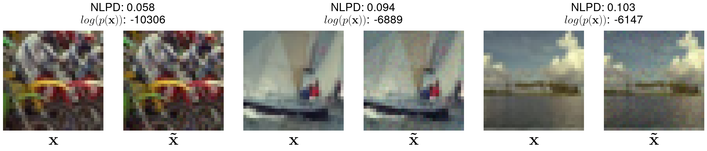
Figure 1: The concept: visual sensitivity may be easy to predict from image probability. Different images are corrupted by uniform noise of the same energy (on the surface of a sphere around ${\bf x}$ of Euclidean radius $\epsilon=1$), with the same RMSE = 0.018 (in [0, 1] range). Due to visual masking (Legge & Foley, 1980), noise of the same energy is more visible, i.e. human sensitivity is bigger, for smooth images. This is consistent with the reported NLPD distance (Laparra et al., 2016), and interestingly, sensitivity is also bigger for more probable images, where $log(p({\bf x}))$ is computed with PixelCNN++ (Salimans et al., 2017).

2.5 A convenient generative model

Our proposal requires a probability model that is able to give an accurate estimate of $p(\mathbf{x})$ at arbitrary points (images) $\mathbf{x}$, so that we can study the sensitivity-probability relation at many images. In this work we rely on PixelCNN++ (Salimans et al., 2017), since it is trained on CIFAR10 (Krizhevsky et al., 2009), a dataset made up of small colour images of a wide range of natural scenes. PixelCNN++ also achieves the lowest negative log-likelihood of the test set, meaning the PDF is accurate in this dataset. This choice is convenient for consistency with previous works (Hepburn et al., 2022) , but note that it is not crucial for the argument made here. In this regard, recent interesting models (Kingma & Dhariwal, 2018; Kadkhodaie et al., 2023) could also be used as probability estimates. Fig. 1 shows that cluttered images are successfully identified as less probable than smooth images by PixelCNN++, consistently with classical results on the average spectrum of natural images (Clarke, 1981; Atick et al., 1992; Malo et al., 2000; Simoncelli & Olshausen, 2001).

2.6 Distorted images

There are two factors to balance when looking for distortions so that the definition of perceptual sensitivity is meaningful. First; in order to understand the ratio in Eq. 1 as a variation per unit of euclidean distortion, we need the distorted image $\tilde{{\bf x}}$ to be close to the original ${\bf x}$. Secondly, the perceptual distances are optimised to recreate human judgements, so if the distortion is too small, such that humans are not able to see it, the distances are not trustworthy.

As such, we propose to use additive uniform noise on the surface of a sphere of radius $\epsilon$ around ${\bf x}$. We choose $\epsilon$ in order to generate $\tilde{{\bf x}}$ where the noise is small but still visible for humans ($\epsilon=1$ in $32\times 32\times 3$ images with colour values in the range [0,1]). Certain radius (or Euclidean distance) corresponds to a unique RMSE, with $\epsilon=1$ RMSE = 0.018 (about $2\%$ of the colour range). Examples of the noisy images can be seen in Fig. 1. Note that in order to use the perceptual distances and PixelCNN++, the image values must be in a specific range. After adding noise we clip the signal to keep that range. Clipping may modify substantially the Euclidean distance (or RMSE) so we only keep the images where $\textrm{RMSE}\in[0.017,0.018]$, resulting in 48,046 valid images out of 50,000.

3 Experiments

Firstly, we empirically show the relation between the sensitivity and the candidate probabilistic factors using conditional histograms, and use information theory measures to tell which factors are most related to the sensitivity. Then, we explore polynomial combinations of several of these factors using regression models. Lastly, we restrict ourselves to the two most important factors and identify simple functional forms to predict perceptual sensitivity.

3.1 Highlighting the relation: Conditional Histograms

Conditional histograms in Fig. 2 illustrate the sensitivities of the metrics conditioned to different probabilistic factors. In this case, the histograms describe the probabilities $\mathcal{P}(S\in[b_{j-1},b_{j}]|X=x)$ where $S$ is certain perceptual sensitivity partitioned into $m=30$ bins $[b_{j-1},b_{j})$, and $X$ is one of the possible probabilistic factors. This allows us to visually inspect which of the probabilistic factors are important for predicting sensitivity. The probabilistic factor used is given in each subplot title alongside with the Spearman correlation between perceptual sensitivity and the factor.

For all perceptual distances, $log(p({\bf x}))$ has a high correlation, and mostly follows a similar conditional distribution. NLPD is the only distance that significantly differs, with more sensitivity in mid-probability images. We also see a consistent increase in correlation and conditional means when looking at $log(p(\tilde{{\bf x}}))$, meaning the log-likelihood of the noisy sample is more indicative of perceptual sensitivity for all tested distances. Also note that the standard deviation $\sigma({\bf x})$ also has a strong (negative) correlation across the traditional distances, falling slightly with the deep learning based approaches. This is likely due to the standard deviation being closely related to the contrast of an image (Peli, 1990), and the masking effect: the sensitivity in known to decrease for higher contrasts (Legge & Foley, 1980; Martinez et al., 2019). Note that measures that take into account both points, $\int^{\tilde{{\bf x}}}_{\bf x}log(p({\bf x}))d{\bf x}$ and $\overrightarrow{J}_{\tilde{x}}({\bf x})$, have lower correlation than just taking into account the noisy sample, with the latter being insignificant in predicting perceptual sensitivity.

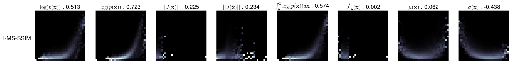
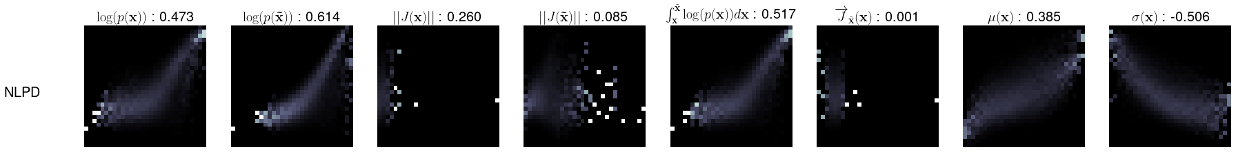
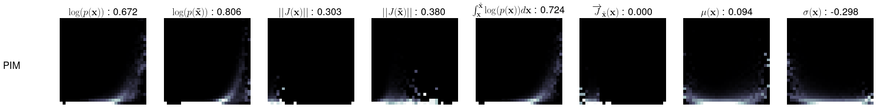
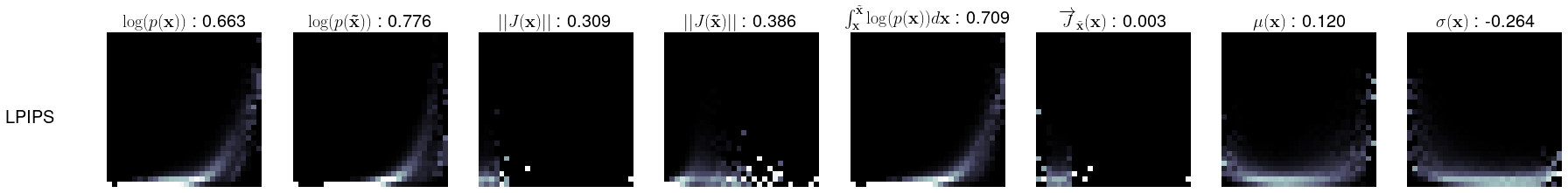
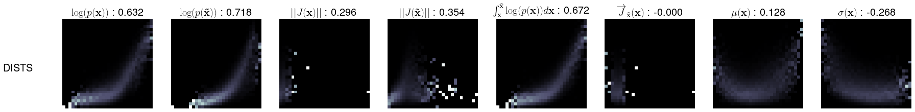
Figure 2: Conditional histograms, x-axis is the probability factor and y-axis is the sensitivity (Eq. 1) of the metric per row. Shown is the Spearman correlation between probabilistic factor and perceptual sensitivity.

3.2 Quantifying the relation: Mutual Information

To quantify the ability of probabilistic factors to predict perceptual sensitivity, we use information theoretic measures. Firstly, we use mutual information which avoids the definition of a particular functional model and functional forms of the features. This analysis will give us insights into which of the factors derived from the statistics of the data can be useful in order to later define a functional model that relates statistics and perception.

The mutual information has been computed using all 48046 samples and using the Rotation Based Iterative Gaussianisation (RBIG) (Laparra et al., 2011) as detailed here (Laparra et al., 2020). Instead of the mutual information value ($I(X,Y)$), we report the Information coefficient of correlation (Linfoot, 1957) (ICC) since the interpretation is similar to the Pearson coefficient and allows for easy comparison, where $\textrm{ICC}(X,Y)=\sqrt{1-e^{-2I(X,Y)}}$.

Figure 3 shows the ICC between each isolated probabilistic factor and the sensitivity of different metrics. It is clear that the most important factor to take into account in most models (second in MS-SSIM) is the probability of the noisy image $\log(p(\tilde{{\bf x}}))$, a consistent result with the conditional histograms.

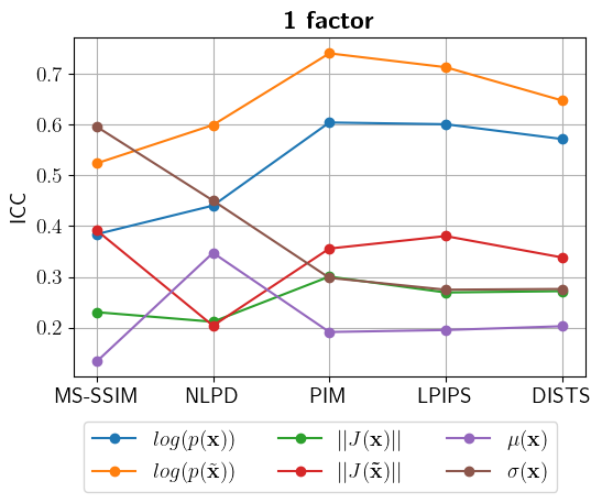
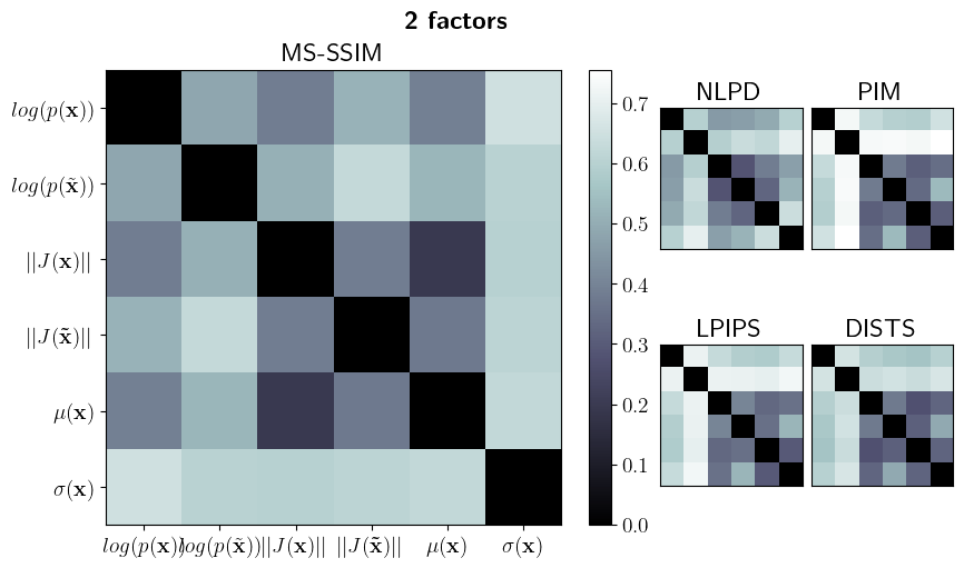
Figure 3: Information Coefficient of Correlation (ICC) between the sensitivity of different perceptual distances and isolated probabilistic factors (left: 1 factor) and different pairs of probabilistic factors (right: 2 factors). The considered factors are explicitly listed at the axes of the matrix of pairs for the MS-SSIM. The meaning of the entries for the matrices of the other distances is the same and all share the same colorbar for ICC.

Once we select the $log(p(\tilde{{\bf x}}))$ as the most important factor, we explore which other factor should be included as the second term. In order to do so we analyse the ICC between each possible combination of two factors with each metric (right panel of Fig. 3). The matrix of possible pairs is depicted in detail for MS-SSIM (with factors in the axes and a colourbar for ICC), and corresponding matrices for the other metrics are also shown in smaller size. We can see that the general trend in four out of five metrics is the same: the pairs where $log(p(\tilde{{\bf x}}))$ is involved have the maximum mutual information. The exception is MS-SSIM, which also behaves differently when using a single factor. In all the other cases the maximum relation with sensitivity is achieved when combining $log(p(\tilde{{\bf x}}))$ with the standard deviation of the original image $\sigma({\bf x})$.

The set of factors found to have a high relation with the variable to be predicted was expanded (one at a time) with the remaining factors. And we computed the mutual information and ICC for such expanded sets of factors. Reasoning as above (Fig. 3, right), we found that the next in relevance was $log(p({\bf x}))$, then the mean $\mu({\bf x})$, then the gradient $||J({\bf x})||$, to finally take into account all the probabilistic factors. Table 2 summarises the increase of ICC (the increase if information about the sensitivity) as we increase the number of probabilistic factors taken into account. In particular, we see that just by using $log(p(\tilde{{\bf x}}))$ we can capture between $[0.55-0.71]$ of the information depending on the metric. Then, for all the metrics, the consideration of additional factors (obviously) improves ICC, but this improvement saturates as new factors contain less independent information about the sensitivity.

Table 2: Information Coefficient of Correlation between the sensitivity and groups of probabilistic factors.

Factors	MS-SSIM	NLPD	PIM	LPIPS	DISTS	mean
1D: $\,\,\,log(p(\tilde{x}))$	0.55	0.57	0.71	0.68	0.61	0.62
2D: {$log(p(\tilde{x}))$, $\sigma(x)$}	0.57	0.66	0.72	0.69	0.63	0.65
3D: {$log(p(\tilde{x}))$, $\sigma(x)$, $log(p({\bf x}))$}	0.68	0.68	0.72	0.69	0.65	0.68
4D: {$log(p(\tilde{x}))$, $\sigma(x)$, $log(p({\bf x}))$, $\mu(x)\}$	0.68	0.76	0.75	0.71	0.66	0.71
5D: {$log(p(\tilde{{\bf x}}))$, $\sigma(x)$, $log(p({\bf x}))$, $\mu(x)$, $||J(x)||$}	0.68	0.78	0.75	0.73	0.66	0.72
6D: all factors	0.71	0.79	0.76	0.73	0.66	0.73

3.3 Accurate but non-interpretable model: non-parametric regression

The ultimate goal of an interpretable explanation of the sensitivity from probabilistic factors is obtaining a simple parametric function of the considered factors that predicts sensitivity. However, simple interpretable models will perform worse than more flexible non-parametric models. Despite the non-interpretability, non-parametric regression is useful to set a reference in performance (upper bound) to assess the quality of the simple interpretable models that we may develop.

In order to estimate this reference in performance, we consider a random forest regressor (Breiman, 2001) to predict the perceptual sensitivity from the probabilistic factors and 2nd order polynomial combinations of the factors. The inverse probability for both original and noisy images is also included. Regression trees are convenient for this task since it is easy to analyse the relevance of each feature and compare between models trained on different perceptual sensitivities. Values of feature importance are normalised so that they sum to $1$ for each model for easy comparison. We use a held out test set of 30% dataset in order to calculate correlations between predicted and ground truth. The average Pearson correlation obtained is 0.85, which serves as an illustrative upper bound reference for the interpretable functions proposed below in Section 3.4. We also trained a simple 3 layer multilayer perceptron on the same data and also achieved a correlation of 0.85.

Figure 5 in Appendix B shows the 6 probabilistic factors with the bigger importance across perceptual distances and their relative relevance for each distance. The Pearson (Spearman) correlations indicate how good the regression models are at predicting sensitivity. $log(p(\tilde{{\bf x}}))$ is by far the most important factor, which agrees with what was found in the mutual information analysis (sec. 3.2). It has been suggested that the derivative of the log-likelihood is important in learning representations (Bengio et al., 2013) since modifications in the slope of the distribution imply label change and the score-matching objective makes use of the gradient. However, we find that this derivative has low mutual information with human sensitivity and low influence in the regression.

3.4 Interpretable model: Simple Functional Forms

In order to get simple interpretable models of sensitivity, in this section we restrict ourselves to linear combinations of power functions of the probabilistic factors. We explore two situations: (1) a single-factor model, and (2) a two-factor model. According to the previous results on the relevance of the factors, the 1-factor model has to be based on $log(p(\tilde{{\bf x}}))$, and the 2-factor model has to be based on $log(p(\tilde{{\bf x}}))$ and $\sigma({\bf x})$.

1-factor model (1F). In the literature, the use of $log(p(\tilde{{\bf x}}))$ has been proposed using different exponents (see table 1). Therefore, first, we analysed which exponents get better results for a single component, i.e. $S({\bf x},\tilde{{\bf x}})=w_{0}+w_{1}~{}log(p(\tilde{{\bf x}}))^{\gamma}$. We found out that there is not a big difference between different exponents. Therefore we decided to go for the simplest solution: a regular polynomial (with natural numbers as exponents). Then, we explored which degree of the polynomial gets better results, and found that going beyond degree 2 does not substantially improve the correlation (detailed results are in Table 4 in Appendix C). We also explore a special situation where factors with different fractional and non-fractional exponents are linearly combined. The best overall reproduction of sensitivity across all perceptual metrics (Pearson correlation 0.73) can be obtained with a simple polynomial of degree two:

$$S({\bf x},\tilde{{\bf x}})=w_{0}+w_{1}~{}log(p(\tilde{{\bf x}}))+w_{2}~{}log(p(\tilde{{\bf x}}))^{2},$$ (3)

where the values for the weights for each perceptual distance are in Appendix D (table 6).

2-factor model (2F). In order to restrict the (otherwise intractable) exploration here we focus on polynomials that include the simpler versions of these factors isolated, i.e. $\{log(p(\tilde{{\bf x}})),log(p(\tilde{{\bf x}}))^{2}\}$ and $\{\sigma({\bf x}),\sigma({\bf x})^{2},\sigma({\bf x})^{-1}\}$, and the simplest products and quotients using both. We perform an ablation search of models that include these combinations as well as a LASSO regression (Tibshirani, 1996) (details in Appendix C (table 5)). In conclusion, a model that combines good predictions and simplicity is the one that simply adds the $\sigma({\bf x})$ factor to the 1-factor model:

$$S({\bf x},\tilde{{\bf x}})=w_{0}+w_{1}~{}log(p(\tilde{{\bf x}}))+w_{2}~{}log(p(\tilde{{\bf x}}))^{2}+w_{3}~{}\sigma({\bf x})$$ (4)

where the values of the weights for the different metrics are in Appendix D (table 7). The 2-factor model obtains an average Pearson correlation of $0.79$ across the metrics, which implies an increase of $0.06$ in correlation in regard to the 1-factor model. As a reference, a model that includes all nine analysed combinations for the two factors achieves an average $0.81$ correlation (not far from the performance obtained with the non-parametric regressor, $0.85$, in section 3.3).

4 Validation: reproduction of classical psychophysics

Variations of human visual sensitivity depending on luminance, contrast, and spatial frequency were identified by classical psychophysics (Weber, 1846; Legge & Foley, 1980; Campbell & Robson, 1968; Georgeson & Sullivan, 1975) way before the advent of the state-of-the-art perceptual distances considered here. Therefore, the reproduction of the trends of those classic behaviours is an independent way to validate the proposed models since it is not related to the recent image quality databases which are at the core of the perceptual distances.

We perform two experiments for this validation: (1) we compute the sensitivity to sinusoidal gratings of different frequencies but the same energy (or contrast), and we do that at different contrast levels, and (2) we compute the sensitivity for natural images depending on luminance and contrast. The first experiment is related to the concept of Contrast Sensitivity Function (CSF) (Campbell & Robson, 1968): the human transfer function in the Fourier domain, just valid for low contrasts, and the decay of such filter with contrast, as shown in the suprathreshold contrast matching experiments Georgeson & Sullivan (1975). The second experiment is related to the known saturation of the response (reduction of sensitivity) for higher luminances: the Weber law (Weber, 1846), and its equivalent (also reduction of the sensitivity) for contrast due to masking (Legge & Foley, 1980).

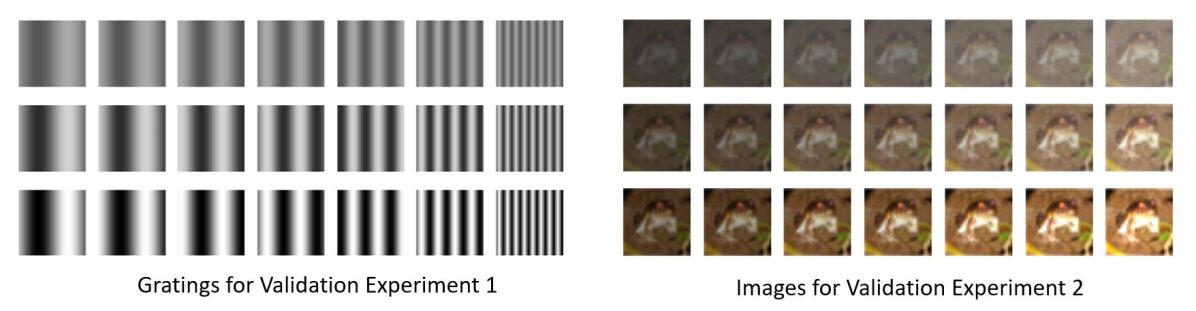
Figure 6: Stimuli for the perceptual tests of the proposed model. (left) Gratings are generated at wavelengths that can be accurately shown in a $32\times 32$ spatial size, generated at contrasts of $[0.2,0.4,0.7]$. (right) Shows one example of editing an image from the CIFAR10 dataset to vary contrast of $[0.2,0.4,0.7]$ and luminance values in $[60,140]$.

Gratings in Experiment 1 were generated with a fixed average luminance of 40 $cd/m^{2}$, and frequencies in the range [1,8] cycles per degree (cpd). We considered three Michelson contrast levels $c=\{0.2,0.4,0.7\}$. Barely visible noise in $\epsilon=1$ sphere was added to the gratings to generate the distorted stimuli $\tilde{{\bf x}}$, and we averaged the sensitivity for 100 samples of the noise. In Experiment 2, we define contrast as $c=\frac{\sigma({\bf x})\sqrt{2}}{\mu({\bf x})}$, which is applicable to natural images and reduces to Michelson contrast for gratings (Peli, 1990). We edited images from CIFAR10 to have the same contrast levels as in Experiment 1 and we explored the range of luminances $[60,140]$ so that the digital values for maximum contrast still were in the [0,255] range. We averaged the sensitivities for 1000 images. Examples of the images for both experiments are given in Fig. 6 in Appendix E. The resulting sensitivities for both experiments are plotted in Fig. 4.

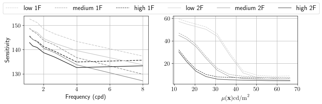
Figure 4: Validation experiment 1 (Contrast Sensitivity Function, left), and validation experiment 2 (Weber law and masking, right) for the 1-factor (1F) and 2-factors (2F) models tuned to the DISTS distance. Color corresponds to the different contrast levels (low=0.2, medium=0.4, high=0.7).

Regarding the sensitivity to gratings (left), results reproduce the decay of the CSF at high frequencies, its decay with contrast, and how the shape flattens with contrast, consistently with (Campbell & Robson, 1968; Georgeson & Sullivan, 1975). For sensitivity at different luminances and contrasts (right) there is a simultaneous reduction in both, consistent with the literature (Weber, 1846; Legge & Foley, 1980). Interestingly, both models 1-F and 2-F follow the same trends. Moreover, given the proportionality between the weights for the different distances (tables 6 and 7 in Appendix D), the trends also hold for all distances.

5 Discussion and Conclusion

We show that several functions of image probability computed from recent generative models share substantial information with the sensitivity of state-of-the-art perceptual metrics (mean ICC of 0.73, Sec. 3.2). Alongside this, a Random Forest regressor that predicts sensitivity from polynomial combinations of these probabilistic factors obtains an average Pearson correlation of 0.85 with actual sensitivity (Sec. 3.3). According to the shared information, the factors can be ranked as: $\{log(p(\tilde{{\bf x}})),\sigma({\bf x}),log(p({\bf x})),\mu({\bf x}),||J({\bf x})||\}$, in agreement with the relevance given by the regression tree that uses the same features. Using only $log(p(\tilde{{\bf x}}))$ obtains an average ICC of 0.62, and a simple quadratic model including only this factor achieves a 0.73 Pearson correlation. This is due to simultaneously including information about the distribution of the original image (in a differential context $p(\tilde{{\bf x}})\approx p({\bf x})$), and also about the specific direction of distortion. After an exhaustive ablation study keeping the factors with the highest ICC values, we propose simple functional forms of the sensitivity-probability relation using just 1 or 2 factors (Eqs. 3 based on $log(p(\tilde{{\bf x}}))$, and Eq. 4 based on $log(p(\tilde{{\bf x}}))$ and $\sigma({\bf x})$). These obtain average Pearson correlations with sensitivity of 0.73 and 0.79 respectively. These simple functions of image probability are validated through the reproduction of trends of the human frequency sensitivity, its suprathreshold variation, the Weber law, and contrast masking (Sec. 4).

This study is limited on the one hand by the probability model used (PixelCNN++), which was trained on a set of small images, with restricted contrast/luminance/color/content range. In order to have trustable $p({\bf x})$ we limited ourselves to using the same kind of (small, limited color range) images. As a proxy for human perception, we used perceptual metrics. Although they correlate with humans, even state-of-the-art metrics are not perfect. The ideal situation would be the direct reproduction of psychophysics (e.g. direct prediction of mean opinion score in image quality databases). However, this is not easy because the images in the subjective experiments usually fall out of the range where you can use the current probability models.

Nevertheless, shared information and correlations are surprisingly high given that the statistics of the environment is not the only in driving factor in vision (Erichsen & Woodhouse, 2012; Sterling & Laughlin, 2015). In fact, this successful prediction of sensitivity from accurate measures of image probability with such simple functional forms is a renewed direct evidence of the relevance of Barlow Hypothesis. Moreover, our results are in contrast with intuitions about the importance of the distribution gradient (Bengio et al., 2013): we found that the gradient of the probability has low shared mutual information and low feature influence in the human sensitivity.

Appendix A Performance of the considered perceptual metrics

Image quality metrics are able to predict visual human perception up to some level. In table 3 we show results of the different image quality metrics used in this work (see sec. 2.4) when evaluated on human rates databases. Although the metrics are not perfect, it is clear that they are a good proxy of human perception. We show results on a traditional perceptual dataset using large images, TID2013 (Ponomarenko et al., 2013), and a more recent dataset with smaller images (size $64\times 64$) but more distortions as using neural networks based ones, such as super-resolution, BAPPS (Zhang et al., 2018).

Table 3: Pearson and Spearman correlations with human opinion in TID2013, and agreement with human judgement (in %) in BAPPS.

	MSSSIM	NLPD	PIM	LPIPS	DISTS
TID2013 $\rho_{p}$ ($\rho_{s}$)	0.78 (0.80)	0.84 (0.80)	0.62 (0.65)	0.74 (0.67)	0.86 (0.83)
BAPPS (%)	61.7	61.5	64.5	69.2	69.0

Appendix B Relevance of factors using random forest regressors.

A random forest regression was fit using multiple combinations of the probability-related factors (see sec. 2.3) to predict the sensitivity of the different image quality metrics used in this work (see sec. 2.4). A total of 55 combinations were introduced as inputs. Figure 5 shows the most relevant ones selected by the random forest algorithm.

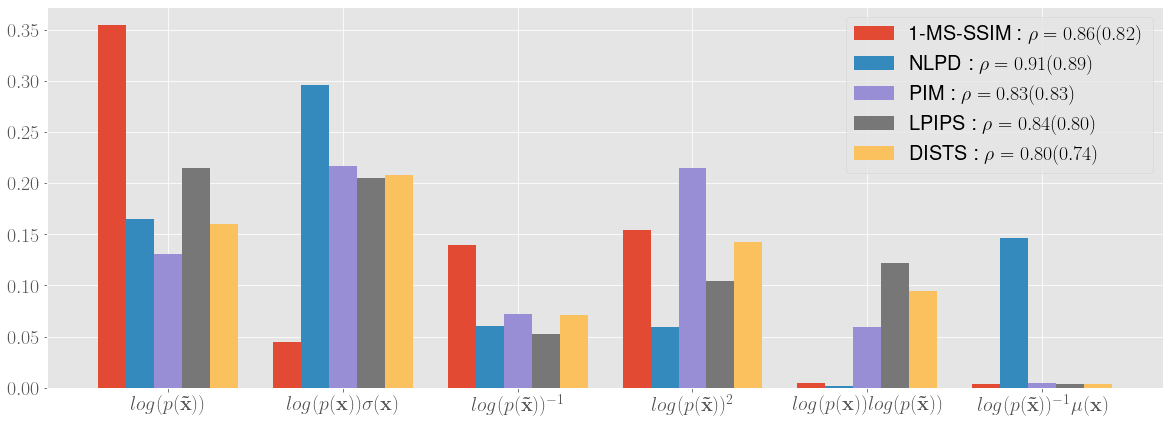
Figure 5: Top 6 feature importance from Random Forest regressors trained on polynomial combinations of the probabilistic factors in order to predict perceptual sensitivity. A separate model was trained for each perceptual distance. In the legend we include the Pearson (Spearman) correlation between the predictions and ground truth for a held out test set 30% of the dataset.

Appendix C Parameter selection for the functional forms.

Here we show the details for the selection of the parameters in section 4. For the one-factor model, we tried different possibilities on the selected factor $log(p(\tilde{{\bf x}}))$, details on the correlation of the different possibilities with sensitivity of perceptual measures are given in table 4 and section 3.4.

Table 4: Pearson correlation obtained between the prediction of the model and the sensitivity for different IQMs. All models are designed using versions of $log(p(\tilde{{\bf x}}))$ as input factor. The models are simple models with only one coefficient, $S({\bf x},\tilde{{\bf x}})=w_{0}+w_{1}~{}log(p(\tilde{{\bf x}}))^{\gamma}$, or polynomials of different degrees (d). The model Frac* is a special polynomial with exponents: [0’3,0’2,0’1,0,1,2,3].

	MSSIM	NLPD	PIM	LPIPS	DISTS	Mean
One coefficient
$\gamma$ = 1/10	0.71	0.64	0.66	0.69	0.72	0.68
$\gamma$ = 1/5	0.71	0.64	0.66	0.69	0.72	0.68
$\gamma$ = 1/3	0.71	0.64	0.66	0.69	0.72	0.68
$\gamma$ = 1/2	0.71	0.63	0.66	0.69	0.72	0.68
$\gamma$ = 2	0.69	0.63	0.64	0.68	0.71	0.67
$\gamma$ = -1	0.72	0.65	0.66	0.71	0.73	0.69
$\gamma$ = 1	0.7	0.63	0.65	0.68	0.72	0.68
Polynomials
d = 2	0.76	0.65	0.75	0.76	0.74	0.73
d = 3	0.76	0.65	0.75	0.75	0.74	0.73
d = 6	0.75	0.64	0.73	0.74	0.74	0.72
Frac*	0.76	0.65	0.76	0.76	0.74	0.73

For the two-factors model, we took the ones obtained in section 4.1 (i.e. $b$ (bias), $log(p(\tilde{{\bf x}}))$, and $log(p(\tilde{{\bf x}}))^{2}$), and factors of the standard deviation $\sigma_{x}$ as suggested by the mutual information in section 3.2. The combinations of the standard deviation have been alone: $\sigma_{x}$, $\frac{1}{\sigma_{x}}$,$\sigma_{x}^{2}$, and combined with the probability of the noisy image: $\frac{log(p(\tilde{{\bf x}}))}{\sigma_{x}}$, $\frac{\sigma_{x}}{log(p(\tilde{{\bf x}}))}$, and $log(p(\tilde{{\bf x}})){\sigma_{x}}$.

There are 9 candidates but we want the most compact and interpretable model. Analysing all the possible combinations is intractable so we are going to perform an ablation study: we are going to discard different candidates sequentially starting from the largest model (9 candidates). Besides, we are going to use LASSO regression with different amounts of regularisation to get models with different amounts of factors as comparison to the ablation study. Results in table 5 are shown in descending number of factors used. For each step, we remove the factor (or factors) that less influence has in the correlation. Besides, we show the correlation given by LASSO models where the regularization parameter has been adjusted in order to have the same number of factors. A model with 6 factors (number 17) has the same correlation (0.81) as the one with all the factors (number 1). The best trade-off between the number of factors and correlation is for models 25, 26, and 27, with 4 factors and a correlation of 0.79. We chose as our final functional model in section 4.2 the model 25 as its factors involve less computations.

Table 5: Linear models using different combinations of $b$ (bias), $log(p(\tilde{x}))=p$ and $\sigma(x)=s$, where $1$ indicates the factor is included in the model, and $0$ it is ablated. Models with $*$ in the model number (# M) have been computed using Lasso and a corresponding regularization parameter in order to have a particular number of combinations (# C). For the perceptual metrics, the Pearson correlation between the predicted and ground truth on a test set of CIFAR10 is reported.

$b$	$p$	$p^{2}$	$s$	$s^{2}$	$\frac{1}{s}$	$\frac{p}{s}$	$\frac{s}{p}$	$ps$	MSSIM	NLPD	PIM	LPIPS	DISTS	Mean	# C	#M
1	1	1	1	1	1	1	1	1	0.85	0.78	0.81	0.81	0.78	0.806	9	1
8 combinations
1	1	1	0	1	1	1	1	1	0.85	0.78	0.8	0.8	0.78	0.802	8	2
1	1	1	1	0	1	1	1	1	0.85	0.78	0.81	0.81	0.78	0.806	8	3
1	1	1	1	1	0	1	1	1	0.85	0.78	0.81	0.81	0.78	0.806	8	4
1	1	1	1	1	1	0	1	1	0.85	0.78	0.81	0.81	0.78	0.806	8	5
1	1	1	1	1	1	1	0	1	0.85	0.78	0.8	0.8	0.78	0.802	8	6
1	1	1	1	1	1	1	1	0	0.85	0.78	0.8	0.8	0.78	0.802	8	7
7 combinations
0	1	1	1	1	1	1	1	0	0.83	0.75	0.77	0.77	0.77	0.778	7	8
1	0	1	1	1	1	1	1	0	0.82	0.78	0.77	0.78	0.77	0.784	7	9
1	1	0	1	1	1	1	1	0	0.82	0.78	0.76	0.77	0.76	0.778	7	10
1	1	1	0	1	1	1	1	0	0.84	0.78	0.8	0.8	0.78	0.8	7	11
1	1	1	1	0	1	1	1	0	0.85	0.78	0.8	0.8	0.78	0.802	7	12
1	1	1	1	1	0	1	1	0	0.85	0.78	0.8	0.8	0.78	0.802	7	13
1	1	1	1	1	1	0	1	0	0.85	0.78	0.8	0.8	0.78	0.802	7	14
1	1	1	1	1	1	1	0	0	0.84	0.78	0.8	0.8	0.78	0.8	7	15
0	1	1	1	1	1	1	0	1	0.84	0.79	0.78	0.8	0.78	0.798	7	16*
6 combinations
1	1	1	1	0	0	0	1	1	0.85	0.78	0.81	0.81	0.78	0.806	6	17
0	1	1	0	1	1	1	0	1	0.84	0.79	0.78	0.8	0.78	0.798	6	18*
5 combinations
1	0	1	1	0	0	0	1	1	0.84	0.78	0.78	0.79	0.77	0.792	5	19
1	1	0	1	0	0	0	1	1	0.84	0.78	0.78	0.79	0.77	0.792	5	20
1	1	1	0	0	0	0	1	1	0.84	0.78	0.8	0.8	0.78	0.8	5	21
1	1	1	1	0	0	0	0	1	0.84	0.78	0.8	0.8	0.78	0.8	5	22
1	1	1	1	0	0	0	1	0	0.84	0.78	0.8	0.8	0.78	0.8	5	23
0	1	1	0	0	1	1	0	1	0.83	0.79	0.78	0.8	0.78	0.796	5	24*
4 combinations
1	1	1	1	0	0	0	0	0	0.83	0.78	0.77	0.78	0.77	0.786	4	25
1	1	1	0	0	0	0	1	0	0.83	0.78	0.78	0.78	0.77	0.788	4	26
1	1	1	0	0	0	0	0	1	0.83	0.78	0.77	0.78	0.77	0.786	4	27
1	1	0	0	0	0	0	1	1	0.8	0.78	0.72	0.74	0.76	0.76	4	28
1	0	1	0	0	0	0	1	1	0.79	0.77	0.7	0.73	0.75	0.748	4	29
0	1	1	1	0	0	0	1	0	0.76	0.65	0.75	0.76	0.74	0.732	4	30
1	0	1	1	0	0	0	1	0	0.79	0.77	0.7	0.72	0.75	0.746	4	31
1	1	0	1	0	0	0	1	0	0.8	0.77	0.71	0.74	0.75	0.754	4	32
0	1	1	0	0	0	1	0	1	0.83	0.79	0.78	0.76	0.77	0.786	4	33*
3 combinations
1	1	1	0	0	0	0	0	0	0.76	0.65	0.75	0.76	0.74	0.732	3	34
1	1	0	0	0	0	0	1	0	0.79	0.77	0.69	0.72	0.75	0.744	3	35
1	1	0	0	0	0	0	0	1	0.78	0.77	0.68	0.71	0.75	0.738	3	36
1	1	0	1	0	0	0	0	0	0.79	0.77	0.69	0.71	0.75	0.742	3	37
1	0	1	0	0	0	0	0	1	0.78	0.77	0.68	0.7	0.74	0.734	3	38
1	0	1	0	0	0	0	1	0	0.78	0.77	0.68	0.71	0.74	0.736	3	39
1	0	1	1	0	0	0	0	0	0.78	0.77	0.68	0.71	0.74	0.736	3	40
1	0	0	0	0	0	0	1	1	0.73	0.75	0.62	0.65	0.7	0.69	3	41
1	0	0	1	0	0	0	1	0	0.74	0.75	0.62	0.65	0.7	0.692	3	42
1	0	0	1	0	0	0	0	1	0.73	0.75	0.61	0.64	0.7	0.686	3	43
0	0	1	0	0	0	1	0	1	0.8	0.78	0.73	0.72	0.75	0.756	3	44*
2 combinations
1	1	0	0	0	0	0	0	0	0.7	0.63	0.65	0.68	0.72	0.676	2	45
1	0	1	0	0	0	0	0	0	0.69	0.63	0.64	0.68	0.71	0.67	2	46
1	0	0	1	0	0	0	0	0	0.43	0.52	0.29	0.28	0.3	0.364	2	47
1	0	0	0	0	0	0	1	0	0.34	0.43	0.21	0.2	0.2	0.276	2	48
1	0	0	0	0	0	0	0	1	0.51	0.59	0.36	0.36	0.38	0.44	2	49
0	0	1	0	0	0	1	0	0	0.71	0.76	0.68	0.71	0.74	0.72	2	50*

Appendix D Coefficients of the functional forms.

In section 4 we propose Eqs. 3 and 4 as estimators of the perceptual sensitivity for 1- and 2-factor models respectively. Note that each metric has a different interpretation of the sensitivity units, therefore the weights of the proposed equations are different for each measure. However the proportion of the weights for each probability factor are almost the same. In tables 6 and 7 we give the actual weights obtained in the experiments for each distance.

Table 6: Coefficients for the Eq. 3 for each metric.

Coefs	MSSIM	NLPD	PIM	LPIPS	DISTS
$w_{0}$	29.5	65	15400	198	161
$w_{1}$	$4.9~{}10^{-3}$	$9.5~{}10^{-3}$	2.62	$3.33~{}10^{-2}$	$2.58~{}10^{-2}$
$w_{2}$	$2.05~{}10^{-7}$	$3.62~{}10^{-7}$	$1.11~{}10^{-4}$	$1.41~{}10^{-6}$	$1.05~{}10^{-6}$

Table 7: Coefficients for the Eq. 4 for each metric.

Coefs	MSSIM	NLPD	PIM	LPIPS	DISTS
$w_{0}$	$28$	$58$	$15100$	$194$	$156$
$w_{1}$	$4.69~{}10^{-3}$	$8.19~{}10^{-3}$	$2.57$	$3.26~{}10^{-2}$	$2.49~{}10^{-2}$
$w_{2}$	$1.96~{}10^{-7}$	$3.09~{}10^{-7}$	$1.09~{}10^{-4}$	$1.37~{}10^{-6}$	$1.00~{}10^{-6}$
$w_{3}$	$-0.597$	$-3.74$	$-141$	$-1.93$	$-2.54$

Appendix E Perceptual tests on the model

Here we show the stimuli used for both perceptual tests performed using the proposed models.

References

- Atick (1992) JJ Atick. Could information theory provide an ecological theory of sensory processing? Network: Computation in Neural Systems, 3(2):213, 1992.
- Atick et al. (1992) JJ. Atick, Z. Li, and AN. Redlich. Understanding retinal color coding from first principles. Neural Comp., 4(4):559–572, 1992.
- Attneave (1954) F. Attneave. Some informational aspects of visual perception. Psychological Review, 61(3), 1954. doi: 10.1037/h0054663.
- Barlow (1961) H. B. Barlow. Possible principles underlying the transformation of sensory messages. Sensory Communication, pp. 217–234, 1961.
- Bell & Sejnowski (1997) Anthony J. Bell and Terrence J. Sejnowski. The ‘independent components’ of natural scenes are edge filters. Vision Research, 37(23):3327–38, 1997.
- Bengio et al. (2013) Yoshua Bengio, Aaron Courville, and Pascal Vincent. Representation learning: A review and new perspectives. IEEE transactions on pattern analysis and machine intelligence, 35(8):1798–1828, 2013. URL http://arxiv.org/abs/1206.5538. cite arxiv:1206.5538.
- Bertalmío et al. (2020) M. Bertalmío, A. Gomez-Villa, and J. et al. Malo. Evidence for the intrinsically nonlinear nature of receptive fields in vision. Scientific Reports, 10:16277, 2020.
- Bhardwaj et al. (2020) S. Bhardwaj, I. Fischer, J. Ballé, and T. Chinen. An unsupervised information-theoretic perceptual quality metric. In Adv. Neur. Inf. Proc. Syst. (NeurIPS), volume 33, pp. 13–24, 2020.
- Breiman (2001) Leo Breiman. Random forests. Machine learning, 45:5–32, 2001.
- Bruce & Tsotsos (2005) Neil Bruce and John Tsotsos. Saliency based on information maximization. In Advances in Neural Information Processing Systems, volume 18. MIT Press, 2005.
- Buchsbaum & Gottschalk (1983) G. Buchsbaum and A. Gottschalk. Trichromacy, opponent colours coding and optimum colour information transmission in the retina. Proc. Roy. Soc. Lond. B Biol. Sci., 220(1218):89–113, 1983.
- Campbell & Robson (1968) F. W. Campbell and J. G. Robson. Application of Fourier analysis to the visibility of gratings. The Journal of Physiology, 197(3):551–566, 1968. URL http://jp.physoc.org/content/197/3/551.abstract.
- Carandini & Heeger (2012) M. Carandini and D. Heeger. Normalization as a canonical neural computation. Nature Reviews. Neurosci., 13(1):51–62, 2012.
- Clarke (1981) R.J. Clarke. Relation between the karhunen loève and cosine transforms. IEE Proc. F, 128(6):359–360, 1981.
- Daly (1990) Scott J. Daly. Application of a noise-adaptive contrast sensitivity function to image data compression. Optical Engineering, 29(8):977 – 987, 1990.
- Ding et al. (2020) K. Ding, K. Ma, S. Wang, and E. P. Simoncelli. Image quality assessment: Unifying structure and texture similarity. arXiv preprint arXiv:2004.07728, 2020.
- Erichsen & Woodhouse (2012) Jonathan T. Erichsen and J. Margaret Woodhouse. Human and Animal Vision, pp. 89–115. Springer London, London, 2012. ISBN 978-1-84996-169-1. doi: 10.1007/978-1-84996-169-1˙3. URL https://doi.org/10.1007/978-1-84996-169-1_3.
- Fechner (1860) Gustav Theodor Fechner. Elements of psychophysics. Volume 1 / Gustav Fechner ; translated by Helmut E. Adler ; edited by David H. Howes, Edwin G. Boring ; with an introduction by Edwin G. Boring. Holt, Rinehart and Winston, Inc., New York, 1860.
- Ganguli & Simoncelli (2014) Deep Ganguli and Eero P. Simoncelli. Efficient sensory encoding and bayesian inference with heterogeneous neural populations. Neural Comput., 26(10):2103–2134, 2014.
- Gegenfurtner & Rieger (2000) Karl R Gegenfurtner and Jochem Rieger. Sensory and cognitive contributions of color to the recognition of natural scenes. Current Biology, 10(13):805–808, 2000.
- Georgeson & Sullivan (1975) M A Georgeson and G D Sullivan. Contrast constancy: deblurring in human vision by spatial frequency channels. The Journal of Physiology, 252(3):627–656, 1975.
- Gomez-Villa et al. (2020) A. Gomez-Villa, A. Martín, J. Vazquez-Corral, M. Bertalmío, and J. Malo. Color illusions also deceive CNNs for low-level vision tasks: Analysis and implications. Vision Research, 176:156 – 174, 2020.
- Hancock et al. (1992) P J B Hancock, R J Baddeley, and L S Smith. The principal components of natural images. Network: Computation in Neural Systems, 3(1):61, 1992.
- Heeger (1992) David Heeger. Normalization of cell responses in cat striate cortex. Vis. Neurosci., 9(2):181–197, 1992.
- Hepburn et al. (2020) Alexander Hepburn, Valero Laparra, Jesús Malo, Ryan McConville, and Raúl Santos-Rodríguez. Perceptnet: A human visual system inspired neural network for estimating perceptual distance. In IEEE ICIP 2020, pp. 121–125. IEEE, 2020.
- Hepburn et al. (2022) Alexander Hepburn, Valero Laparra, Raul Santos-Rodriguez, Johannes Ballé, and Jesus Malo. On the relation between statistical learning and perceptual distances. In Int. Conf. Learn. Repr. (ICLR), 2022. URL https://openreview.net/forum?id=zXM0b4hi5_B.
- Hillis & Brainard (2005) James M. Hillis and David H. Brainard. Do common mechanisms of adaptation mediate color discrimination and appearance? uniform backgrounds. J. Opt. Soc. Am. A, 22(10):2090–2106, 2005.
- Hyvärinen et al. (2009) Aapo Hyvärinen, Jarmo Hurri, and Patrick O Hoyer. Natural image statistics: A probabilistic approach to early computational vision., volume 39. Springer Science & Business Media, 2009.
- Kadkhodaie et al. (2023) Zahra Kadkhodaie, Florentin Guth, Stéphane Mallat, and Eero P Simoncelli. Learning multi-scale local conditional probability models of images. In The Eleventh International Conference on Learning Representations, 2023.
- Kingma & Dhariwal (2018) Durk P Kingma and Prafulla Dhariwal. Glow: Generative flow with invertible 1x1 convolutions. Advances in neural information processing systems, 31, 2018.
- Krizhevsky et al. (2009) A. Krizhevsky, G. Hinton, et al. Learning multiple layers of features from tiny images. 2009.
- Laparra & Malo (2015) V. Laparra and J. Malo. Visual aftereffects and sensory nonlinearities from a single statistical framework. Frontiers in Human Neuroscience, 9:557, 2015. doi: 10.3389/fnhum.2015.00557.
- Laparra et al. (2010) V. Laparra, J. Muñoz-Marí, and J. Malo. Divisive normalization image quality metric revisited. J. Opt. Soc. Am. A, 27(4):852–864, 2010.
- Laparra et al. (2012) V. Laparra, S. Jiménez, G. Camps, and J. Malo. Nonlinearities and adaptation of color vision from sequential principal curves analysis. Neural Comp., 24(10):2751–2788, 2012.
- Laparra et al. (2016) V. Laparra, J Ballé, A Berardino, and Simoncelli E P. Perceptual image quality assessment using a normalized laplacian pyramid. Electronic Imaging, 2016(16):1–6, 2016.
- Laparra et al. (2011) Valero Laparra, Gustavo Camps-Valls, and Jesús Malo. Iterative gaussianization: from ica to random rotations. IEEE transactions on neural networks, 22(4):537–549, 2011.
- Laparra et al. (2020) Valero Laparra, J Emmanuel Johnson, Gustau Camps-Valls, Raul Santos-Rodríguez, and Jesus Malo. Information theory measures via multidimensional gaussianization. arXiv preprint arXiv:2010.03807, 2020.
- Laughlin (1981) S. Laughlin. A simple coding procedure enhances a neuron’s information capacity. Zeit. Natur. C, Biosciences, 36(9-10):910—912, 1981. ISSN 0341-0382.
- Legge & Foley (1980) Gordon E. Legge and John M. Foley. Contrast masking in human vision. J. Opt. Soc. Am., 70(12):1458–1471, Dec 1980.
- Li et al. (2022) Qiang Li, Alex Gomez-Villa, Marcelo Bertalmío, and Jesús Malo. Contrast sensitivity functions in autoencoders. Journal of Vision, 22(6), 05 2022. doi: 10.1167/jov.22.6.8.
- Linfoot (1957) E.H. Linfoot. An informational measure of correlation. Information and Control, 1(1):85–89, 1957. ISSN 0019-9958. doi: https://doi.org/10.1016/S0019-9958(57)90116-X. URL https://www.sciencedirect.com/science/article/pii/S001999585790116X.
- Lloyd (1982) S. Lloyd. Least squares quantization in pcm. IEEE Transactions on Information Theory, 28(2):129–137, 1982.
- Macleod & von der Twer (2003) Donald Ia Macleod and Tassilo von der Twer. The pleistochrome: Optimal opponent codes for natural colours. In Mausfeld and Heyer (eds.), Colour Perception: Mind and the Physical World. Oxford University Press, 2003.
- Macq (1992) B. Macq. Weighted optimum bit allocations to orthogonal transforms for picture coding. IEEE Journal on Selected Areas in Communications, 10(5):875–883, 1992.
- Malo & Laparra (2010) J. Malo and V. Laparra. Psychophysically tuned divisive normalization approximately factorizes the pdf of natural images. Neural computation, 22(12):3179–3206, 2010.
- Malo et al. (1997) J. Malo, A.M. Pons, and J.M. Artigas. Subjective image fidelity metric based on bit allocation of the human visual system in the dct domain. Image and Vision Computing, 15(7):535–548, 1997.
- Malo et al. (2000) J. Malo, F. Ferri, J. Albert, J. Soret, and J.M. Artigas. The role of perceptual contrast non-linearities in image transform quantization. Image and Vision Computing, 18(3):233–246, 2000.
- Malo et al. (2021) J. Malo, B. Kheravdar, and Q. Li. Visual information fidelity with better vision models and better mutual information estimate. J. Vision, 21(9):2351, 2021. ISSN 0019-9958. doi: 10.1167/jov.21.9.2351.
- Malo & Gutiérrez (2006) Jesús Malo and Juan Gutiérrez. V1 non-linear properties emerge from local-to-global non-linear ica. Network: Computation in Neural Systems, 17(1):85–102, 2006.
- Marr & Poggio (1976) David Marr and Tomaso Poggio. From understanding computation to understanding neural circuitry. AI Memo No. AIM-357. MIT Libraries, 1976. URL http://hdl.handle.net/1721.1/5782.
- Martinez et al. (2018) M. Martinez, P. Cyriac, T. Batard, M. Bertalmío, and J. Malo. Derivatives and inverse of cascaded linear+ nonlinear neural models. PLoS ONE, 13(10):e0201326, 2018.
- Martinez et al. (2019) M. Martinez, M. Bertalmío, and J. Malo. In praise of artifice reloaded: Caution with image databases in modeling vision. Front. Neurosci., 13:1–17, 2019.
- Michelson (1927) AA. Michelson. Studies in Optics. U. Chicago Press, Chicago, Illinois, 1927.
- Miyasawa (1961) K. Miyasawa. An empirical bayes estimator of the mean of a normal population. Bull. Inst. Internat. Statist., 38:181––188, 1961.
- Olshausen & Field (1996) B.A. Olshausen and D.J. Field. Emergence of simple-cell receptive field properties by learning a sparse code for natural images. Nature, 381:607–609, June 1996.
- Peli (1990) Eli Peli. Contrast in complex images. J. Opt. Soc. Am. A, 7(10):2032–2040, 1990.
- Ponomarenko et al. (2013) N. Ponomarenko et al. Color image database tid2013: Peculiarities and preliminary results. In EUVIP, pp. 106–111. IEEE, 2013.
- Purves et al. (2011) Dale Purves, William T. Wojtach, and R. Beau Lotto. Understanding vision in wholly empirical terms. Proc. Nat. Acad. Sci., 108(supplement_3):15588–15595, 2011.
- Raphan & Simoncelli (2011) Martin Raphan and Eero P. Simoncelli. Least Squares Estimation Without Priors or Supervision. Neural Comp., 23(2):374–420, 02 2011.
- Salimans et al. (2017) T. Salimans, A. Karpathy, X. Chen, and D. P. Kingma. PixelCNN++: Improving the pixelcnn with discretized logistic mixture likelihood and other modifications. arXiv preprint arXiv:1701.05517, 2017.
- Schwartz & Simoncelli (2001) O. Schwartz and E. Simoncelli. Natural signal statistics and sensory gain control. Nature Neurosci., 4(8):819–825, 2001.
- Seriès et al. (2009) Peggy Seriès, Alan A. Stocker, and Eero P. Simoncelli. Is the Homunculus “Aware” of Sensory Adaptation? Neural Computation, 21(12):3271–3304, 12 2009.
- Shannon (1948) Claude Elwood Shannon. A mathematical theory of communication. The Bell System Technical Journal, 27:379–423, 1948.
- Sheikh & Bovik (2006) H. Sheikh and A. Bovik. Image information and visual quality. IEEE Trans. Im. Proc., 15(2):430–444, Feb 2006.
- Simoncelli & Olshausen (2001) Eero P Simoncelli and Bruno A Olshausen. Natural image statistics and neural representation. Annual review of neuroscience, 24(1):1193–1216, 2001.
- Simoncelli (1997) E.P. Simoncelli. Statistical models for images: compression, restoration and synthesis. In Conference Record of the Thirty-First Asilomar Conference on Signals, Systems and Computers (Cat. No.97CB36136), volume 1, pp. 673–678 vol.1, 1997. doi: 10.1109/ACSSC.1997.680530.
- Sterling & Laughlin (2015) Peter Sterling and Simon Laughlin. Principles of Neural Design. The MIT Press, 05 2015.
- Teo & Heeger (1994) P. Teo and D. Heeger. Perceptual image distortion. In IEEE ICIP, volume 2, pp. 982–986, 1994.
- Tibshirani (1996) Robert Tibshirani. Regression shrinkage and selection via the lasso. Journal of the Royal Statistical Society: Series B (Methodological), 58(1):267–288, 1996.
- Twer & MacLeod (2001) T. Twer and D. MacLeod. Optimal nonlinear codes for the perception of natural colours. Network: Comp. Neur. Syst., 12(3):395–407, 2001.
- van den Oord & Schrauwen (2014) Aäron van den Oord and Benjamin Schrauwen. The student-t mixture as a natural image patch prior with application to image compression. Journal of Machine Learning Research, 15(60):2061–2086, 2014.
- van den Oord et al. (2016) Aäron van den Oord, Nal Kalchbrenner, and Koray Kavukcuoglu. Pixel recurrent neural networks. CoRR, abs/1601.06759, 2016.
- Vincent (2011) Pascal Vincent. A Connection Between Score Matching and Denoising Autoencoders. Neural Comp., 23(7):1661–1674, 07 2011.
- Wang et al. (2003) Z. Wang, E. P. Simoncelli, and A. C. Bovik. Multiscale structural similarity for image quality assessment. In ACSSC, volume 2, pp. 1398–1402. Ieee, 2003.
- Wang et al. (2004) Z. Wang, A. C. Bovik, H. R. Sheikh, and E. P. Simoncelli. Image quality assessment: from error visibility to structural similarity. IEEE Trans. Image Process, 13(4):600–612, April 2004. ISSN 1057-7149. doi: 10.1109/TIP.2003.819861.
- Wang & Bovik (2009) Zhou Wang and Alan C. Bovik. Mean squared error: Love it or leave it? a new look at signal fidelity measures. IEEE Signal Processing Magazine, 26(1):98–117, 2009. doi: 10.1109/MSP.2008.930649.
- Watson (1993) A.B. Watson. Digital images and human vision. Cambridge, Mass. : MIT Press, 1993.
- Weber (1846) E. H. Weber. The sense of touch and common feeling, 1846, pp. 194–196. Appleton-Century-Crofts, NY, 1846. doi: 10.1037/11304-023.
- Whittle (1992) Paul Whittle. Brightness, discriminability and the “crispening effect”. Vision Research, 32(8):1493–1507, 1992.
- Wichmann et al. (2002) F.A. Wichmann, L.T. Sharpe, and K.R. Gegenfurtner. The contributions of color to recognition memory for natural scenes. J. Experim. Psychol.: Learn., Memory, and Cognit., 28(3):509–520, 2002.
- Zhang et al. (2018) R. Zhang, P. Isola, A. Efros, E. Shechtman, and O. Wang. The unreasonable effectiveness of deep features as a perceptual metric. In Proceedings of the IEEE CVPR, pp. 586–595, 2018.