Algebraic Compression of Free Fermionic Quantum Circuits:
Particle Creation, Arbitrary Lattices and Controlled Evolution

Abstract

Recently we developed a local and constructive algorithm based on Lie algebraic methods for compressing Trotterized evolution under Hamiltonians that can be mapped to free fermions [1, 2]. The compression algorithm yields a circuit which scales linearly in the number of qubits, is fixed depth for for arbitrarily long evolution times and is applicable to time dependent Hamiltonians, although is limited to simple nearest-neighbor spin interactions and fermionic hopping. In this work, we extend the algorithm to compress circuits simulating evolution with long-range spin interactions and fermionic hopping, thereby enabling embedding of arbitrary lattices onto a chain of qubits. Moreover, we show that controlled time evolution, as well as fermion creation and annihilation operators can also be compressed. We demonstrate our results by adiabatically preparing the ground state for a half-filled fermionic chain, and simulating a $4\times 4$ tight binding model on ibmq_washington. With these new developments, our results enable the simulation of a wider range of models of interest and the efficient compression of subcircuits.

I Introduction

Time evolution of a quantum state is one of the potential areas where quantum computers are expected to have an advantage over classical computers; while state preparation lies in the QMA complexity class, time evolution is part of the simpler BQP class. Importantly for applications in physics and chemistry, time evolution is a building block for quantum simulation of physical and chemical systems. It underpins state preparation via adiabatic time evolution, and is a critical step in determining dynamic response functions [3, 4, 5, 6, 7, 8, 9, 10]. Furthermore, time evolution under a piecewise contant Hamiltonian has also garnered some recent interest in the context of Floquet dynamics and phase transitions [11, 12, 13].

In all cases, a crucial challenge remains: How do we implement the time evolution operator $U(t)$ on a digital quantum computer? The Hamiltonian is typically a sum of Pauli strings $\sigma_{k}$,

$$\mathcal{H}(t)=\sum_{k}\alpha_{k}(t)\sigma_{k},$$ (1)

where $\alpha_{k}(t)$ are real functions of time $t$, and $U(t)$ is related to the Hamiltonian $\mathcal{H}(t)$ via the following equation

$$\partial_{t}U(t)=-i\mathcal{H}(t)U(t),$$ (2)

with initial condition $U(t=0)=\mathcal{I}$. In the simplest case, when the Hamiltonian $\mathcal{H}$ is time independent $U(t)=\exp(-i\mathcal{H}t)$. However, the Pauli strings $\sigma_{k}$ in the Hamiltonian Eq. 1 usually do not commute with each other, and thus $U(t)$ cannot be directly decomposed into the 1- and 2-qubit gates that are available on a quantum computer. Finding such a decomposition for $U(t)$ is entitled unitary synthesis, and is a difficult problem that generally scales exponentially in the number of qubits [14].

A natural choice for decomposition which covers the time dependent case as well, is by use of Trotterization, or expansion of the time evolution operator into small time steps $\delta t$,

$$U(t)\approx\underbrace{e^{-i\mathcal{H}(t_{1})\delta t}e^{-i\mathcal{H}(t_{2})\delta t}\cdots e^{-i\mathcal{H}(t_{N})\delta t}}_{N\,\mathrm{time\>steps}},$$ (3)

where $t_{n}=n\delta t$ and $\delta t=t/N$. This has the added advantage that the individual small time steps can be broken up to separate the Pauli strings

$$e^{-i\mathcal{H}(t_{n})\delta t}\approx\prod_{k}e^{-i\alpha_{k}(t_{n})\sigma_{k}\delta t}+\mathcal{O}(\delta t^{2}),$$ (4)

which leads to a natural circuit implementation. The downside of this approach is that the circuit depth grows with simulation time $t$, which is undesirable for current era noisy quantum computers.

There are a variety of methods proposed to overcome or bypass the problems that arise from the deep circuits from a naïve Trotter implementation. These include variational approaches to learn shorter circuits [15, 16], and decompositions based on algebraic methods that do not grow as a function of simulation time [17, 18, 19, 20, 1, 2].

In general, due to no-go theorems on fast-forwarding quantum evolution, these circuits may be exponentially deep [21, 22, 23]. However, for Hamiltonians that can be mapped onto free fermionic ones, shallow fixed depth circuits, that are independent of simulation time, exist [1, 2, 24, 25, 26, 27, 28]. Previous work by the authors and others have demonstrated that the circuit elements that arise from evolution under a 1D nearest-neighbor free fermionic Hamiltonian obey three algebraic properties — fusion, commutation and turnover — which can be used for an efficient compression algorithm that results in a fixed-depth circuit. While the class of free fermionic Hamiltonians is somewhat restrictive, since it includes some of the more common ones studied in quantum computing — such as the nearest-neighbor transverse field Ising model (TFIM) and nearest-neighbor transverse field XY model (TFXY) — the compression algorithm in applications[29, 10], or has otherwise set a benchmark for what comprises a minimal circuit[30, 31, 32, 33, 34]. Since the compression algorithm starts from a Trotter decomposition, it readily handles evolution under a time-dependent Hamiltonian as well. Moreover, the circuit compression is not limited to time evolution, but is applicable to any circuit elements that obey a few key relationships. Thus, the compression algorithm can also be used for subcircuits built of free fermionic operators. This situation arises regularly because part of interacting fermionic evolution is free fermion hopping.

Figure 1: Summary of the results from Refs. [1, 2] that we will use in this work. Panels (a-c) illustrate the block properties listed in Def. 1. Panel (d) illustrates the triangle structure and how it can absorb a block via the block properties. Panel (e) is an illustration of the usage of block properties to transform a triangle into a shallower square structure. Panels (f) and (g) illustrate two different realizations or representations of the abstract block objects as circuit elements for transverse field Ising model (TFIM) and transverse field XY (TFXY) model.

In this paper, we extend our previous compression work in four ways. We show that (i) long-range fermionic hopping can be compressed, (ii) single particle creation/annihilation operators can be compressed, (iii) fermionic swap (FSWAP) operators can be compressed, and (iv) singly-controlled free fermionic evolution can be compressed.

These developments, when combined, lead to a number of significant improvements and enhanced capabilities of our approach. First, long-range hopping and FSWAP compression enables the compression of free fermionic evolution on any lattice, not just linear chains. Moreover, the FSWAP operator is key in any situation where fermionic statistics matter. Second, compressing single-particle creation operators combines the preparation of a free fermionic or Hartree-Fock state into the time evolution. And finally, controlled evolution is an important yet difficult problem, and we show that it is possible to compress as long as there is a single control ancilla. The most notable application is the compression of Hadamard-test style circuits, where wave function overlaps need to be measured.

In this paper, we outline the mathematical developments required for these enhanced capabilities. We demonstrate the use of the compression of creation/annihilation operators for state preparation by selecting the appropriate particle number sector in a one-dimensional free fermionic chain. Finally, we report the results of a 16 qubit simulation of a 2D free fermionic evolution on a $4\times 4$ lattice using IBM quantum computers which shows exceptionally good fidelity both in the ordered and disordered regime.

The compression software is available as part of the fast free fermion compiler (F3C) [35, 36] at https://github.com/QuantumComputingLab. F3C is based on the QCLAB toolbox [37, 38] for creating and representing quantum circuits.

II Summary of the results

In Refs. [1, 2] we posited the existence of a structure called a “block” ${B}$ that may represent any number and type of quantum circuit elements. A block has an index $i$ and one or more parameters $\bm{\theta}$, which we often write as $B_{i}(\bm{\theta})$. A block satisfies three key properties that allow for compression:

Definition 1 (Block).

Define a “block” $B_{i}(\bm{\theta})$ as a structure that satisfies the following three properties:

1. Fusion: for any set of parameters $\bm{\alpha}$ and $\bm{\beta}$, there exist $\bm{a}$ such that

   $$B_{i}(\bm{\alpha})\,B_{i}(\bm{\beta})=B_{i}(\bm{a}),$$ (5)

2. Commutation: for any set of parameters $\bm{\alpha}$ and $\bm{\beta}$

   $$B_{i}(\bm{\alpha})\,B_{j}(\bm{\beta})=B_{j}(\bm{\beta})\,B_{i}(\bm{\alpha}),\qquad|i-j|>1,$$ (6)

3. Turnover: for any set of parameters $\bm{\alpha}$, $\bm{\beta}$ and $\bm{\gamma}$ there exist $\bm{a}$, $\bm{b}$ and $\bm{c}$ such that

   $$B_{i}(\bm{\alpha})\,B_{i+1}(\bm{\beta})\,B_{i}(\bm{\gamma})=B_{i+1}(\bm{a})\,B_{i}(\bm{b})\,B_{i+1}(\bm{c}).$$ (7)

These properties are summarized in Fig. 1 panels (a-c). With these properties, we have shown that any product that consist of only blocks can be compressed to a triangle, also indicated in Fig. 1 panel (d), where the block on the right follows the red line down –by means of repeated turnover operations– and fuses with the block at the end of the line. After that as shown in panel (e) the triangle at hand can be transformed into a shallower structure called square via block properties.

In order to show that a set of quantum circuit elements can be compressed it suffices to establish a block mapping, i.e., showing that the circuit elements obey the three properties. In our original work, we demonstrated block mappings that arise in the Trotterized quantum circuits for time evolution of three models: the transverse field Ising model (TFIM), the transverse field XY model (TFXY), and the Kitaev model. TFIM and TFXY block mappings are illustrated in Fig. 1 panel (f) and (g). Via the Jordan-Wigner transformation, this enables compressed free fermionic evolution under a Hamiltonian for an $n$-site chain of free fermions

$$\mathcal{H}(t)=\sum_{i=1}^{n-1}\big{(} h_{i}(t)c_{i}^{\dagger}c_{i+1}+p_{i}(t)c_{i}c_{i+1}\big{)}+\mathrm{h.c.}$$ (8)

where $h_{i}(t)$ and $p_{i}(t)$ are complex numbers, and $c_{i}(c_{i}^{\dagger})$ is a fermion annihilation(creation) operator on site $i$.

In this work, we extend the previous results in two significant directions:

II.1 New $B$-block mappings

As we will shortly introduce a second block mapping, we will refer to blocks satisfying Def. 1 as $B$-blocks.

1. We establish a $B$-block mapping for fermionic SWAP operators. This enables compression of fermion swap networks, and establishes that long-range hopping can be compressed.

2. We establish a $B$-block mapping for fermion creation/annihilation operators. This enables the incorporation of particle number changes into the compressed circuit.

Together, these generalize the compressible evolution Hamiltonian to

$$\mathcal{H}(t)=\sum_{i,j}\big{(}h_{ij}(t)\,c_{i}^{\dagger}c_{j}+p_{ij}(t)\,c_{i}c_{j}+q_{i}(t)\,c_{i}\big{)}+\mathrm{h.c.}$$ (9)

where the quadratic fermionic operators now connect any two sites, and single fermionic operators appear.

II.2 $P$-blocks and mappings

1. We define a new type of block, called $P$, with its own properties and relationships to $B$-blocks. Similarly to $B$-blocks, these can be efficiently compressed.

2. We establish a $P$-block mapping for controlled operations, specifically showing that a controlled TFXY $B$-block can be implemented via a $P$-block mapping.

This extends the compressible Hamiltonians into the following form

$$\begin{split}\mathcal{H}_{\mathrm{full}}(t)&=\sum_{i,j}\big{(}u_{ij}(t)c_{i}^{\dagger}c_{j}+v_{ij}(t)c_{i}c_{j}+\text{H.c.}\big{)}\\ &+\sum_{i,j}\big{(}u^{\prime}_{ij}(t)Z_{0}c_{i}^{\dagger}c_{j}+v^{\prime}_{ij}(t)Z_{0}c_{i}c_{j}+\text{H.c.}\big{)}.\end{split}$$ (10)

which include free fermionic evolution controlled via one ancilla qubit.

III Compressing Free Fermionic Evolution

In this section, we detail the mathematical developments. First, we review the results of our previous work on nearest neighbor fermionic hopping [1, 2]. We follow this with the details for compressing creation and annihilation operators in Sec. III.2, compressing fermionic long-range hopping and fermionic swap gates in Sec. III.3.

III.1 Review of Nearest-Neighbor Fermionic Hopping

The block mappings, first introduced in [1, 2], that we will be focusing on in this paper are the TFIM and TFXY block mappings. Mathematically, the TFIM block mapping is given by,

$$\begin{split}B^{\mathrm{TFIM}}_{2i-1}(\theta)&=e^{i\theta Z_{i}},\\ B^{\mathrm{TFIM}}_{2i}(\theta)&=e^{i\theta X_{i}X_{i+1}},\end{split}$$ (11)

and the TFXY blocks are,

$$\begin{split}B^{\mathrm{TFXY}}_{i}(\bm{\theta})=\ &e^{i\theta_{1}\>Z_{i}}e^{i\theta_{2}\>Z_{i+1}}e^{i\theta_{3}\>X_{i}X_{i+1}}\\ &e^{i\theta_{4}\>Y_{i}Y_{i+1}}\>e^{i\theta_{5}\>Z_{i}}e^{i\theta_{6}\>Z_{i+1}}.\end{split}$$ (12)

Fig. 1 panels (f) and (g) illustrates these mappings in terms of $Z$, $XX$ and $YY$ rotation gates.

It was proven in Ref. [1] that the mappings Eq. 11 and Eq. 12 obey the block rules. Note that we have drawn the TFIM mapping in gray and the TFXY mapping in turquoise to distinguish them from each other, and we have drawn the qubit lines to distinguish these concrete mappings from the abstract block structure.

These two block mappings are equivalent to each other and can be used interchangeably, TFXY blocks can be transformed to TFIM blocks and vice versa. For example, a conversion from TFIM to TFXY can be done as shown here

(13)

where we have used the TFIM block mapping, regrouped these as TFXY blocks, and used the TFXY merge operation. The reverse conversion is easier to realize: a $YY$ rotation is just an $XX$ rotation with additional $Z$ rotations on both qubits, thus

(14)

The two mappings have their own advantages: the TFXY mapping only requires half the number of CNOTs of the TFIM mapping because $XX$ rotation followed by $YY$ rotation can be implemented via 2 CNOTs [39], where as the same structure with TFIM require 4 CNOTs in general. On the other hand, compressing a TFIM mapping is approximately 20 times faster and more straightforward [2]. Throughout the paper we will mostly be using the TFXY mapping for circuits in order to minimize the number of CNOTs of the generated circuits.

The TFIM and TFXY models are connected to free fermions via the Jordan-Wigner transformation:

$$\begin{split}c_{n}&=\frac{1}{2}Z_{1}Z_{2}...Z_{n-1}(X_{n}-iY_{n}),\\ c_{n}^{\dagger}&=\frac{1}{2}Z_{1}Z_{2}...Z_{n-1}(X_{n}+iY_{n}).\end{split}$$ (15)

Then, for example, we have

$$\begin{split}c^{\dagger}_{n}c_{n+1}+\mathrm{h.c.}=&-\frac{1}{2}\left(X_{n}X_{n+1}+Y_{n}Y_{n+1}\right),\\ c^{\dagger}_{n}c_{n}=&-\frac{1}{2}\left(I-Z_{n}\right).\end{split}$$ (16)

In a similar way, $X_{n}X_{n+1}$, $Y_{n}X_{n+1}$, $X_{n}Y_{n+1}$, and $Y_{n}Y_{n+1}$ can be written as a linear combination of $c^{(\dagger)}_{n}c^{(\dagger)}_{n+1}$ terms. With this, we have shown that the TFIM and TFXY block mappings can be used to compress time evolution circuit for any time dependent, free fermionic Hamiltonian on a 1D open chain that with nearest-neighbor hopping $c_{i+1}^{\dagger}c_{i}$, nearest-neighbor pair creation (annihilation) $c_{i+1}c_{i}$ ($c_{i+1}^{\dagger}c_{i}^{\dagger}$) and onsite potential $c_{i}^{\dagger}c_{i}$ terms.

III.2 Fermion Annihilation / Creation

In this section, we demonstrate that the preparation of a product state of any number of free fermionic states can be compressed. Consider the following Hamiltonian on a 1-D $n$-site open chain:

$$\mathcal{H}(t)=\sum_{i=1}^{n-1}\big{(} h_{i}(t)\,c_{i}^{\dagger}c_{i+1}+p_{i}(t)\,c_{i}c_{i+1}\big{)}+q(t)\,c_{1}+\text{h.c.},$$ (17)

where $h_{i}(t)$, $p_{i}(t)$ and $q(t)$ are complex functions of time. The difference between this Hamiltonian and Eq. 8 is the presence of the first order terms $c_{1}$ and $c_{1}^{\dagger}$, which annihilates (resp. creates) fermions on site $1$. The standard TFIM and TFXY mappings from Eqs. 11 and 12 cover all the terms in Eq. 17 except for $c_{1}$ and $c_{1}^{\dagger}$. In Appendix B, we show that adding $B^{\mathrm{TFIM}}_{0}:=\exp(i\>\theta X_{1})$ to the TFIM block mapping preserves all block properties and is a valid $B$-block mapping which covers $c_{1}$ term in the Hamiltonian (17) for any complex function of time $q(t)$.

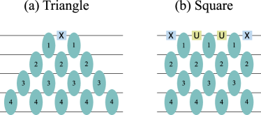
Figure 2: (a) Triangle and (b) square structures for the compression of the Hamiltonian with creation/annihilation operatorss (Eq. 17) for system size $n=4$. The compression is done via TFIM blocks, and then it is transformed into TFXY blocks via Eq. 13 to reduce the CNOT count. See Appendix B for a detailed discussion.

Figure 3: Panel (a) illustrates the compression of $r$ Trotter steps of the long-range hoppings in the Hamiltonian Eq. 18 into a square made out of TFXY blocks $B^{\mathrm{TFXY}}_{i}$. We have used stretched TFXY blocks to illustrate the long range hoppings. Panel (b) illustrates the compression of $r$ Trotter steps long-range hoppings and creation/annihilation on every site in the Hamiltonian in Eq. 25 into a square made out of TFXY blocks $B^{\mathrm{TFXY}}_{i}$ and single qubit rotations.

This new mapping enables compression of single particle creation/annihilation on one edge of the chain consisting of lattices labeled with $1,2,3,...,n$. As in our previous works [1, 2], we can produce two types of fixed depth circuits for this model, triangle and square, which are illustrated in Fig. 2 where U rotations are generic 1-qubit rotations (details of compression and the fixed depth circuits for this model can be found in Appendix B). For an $n$-site system, considering that each TFXY block require 2 CNOTs, the number of CNOTs for both of these circuits can be calculated as $(n+2)(n+1)$.

In order to produce multiple fermionic states, one generates a triangle structure (Fig. 2(a)) for each fermion, which are subsequently compressed to a single one via the block rules (c.f. Fig. 3). Thus, although the Hamiltonian in Eq. 17 has only one creation operator, the time evolution unitary applies the creation/annihilation operators repeatedly. TFXY blocks are capable of creating particle pairs via $XX$ and $YY$ rotations, and can change the particle number by an even number. The addition of one $X$ rotation gate allows us to change the particle number via odd amounts as well, thus giving us full control of the particle content. In other words, while seeing only one $X$ rotation on the triangle might seem to be limited to creating one particle, this structure can create or annihilate any number of particles.

III.3 Fermionic Swap Gate and Long-Range Hoppings

We next show that the TFXY and TFIM block mappings can compress any free fermionic Hamiltonian with long-range hoppings,

$$\mathcal{H}(t)=\sum_{i,j}\big{(}h_{ij}(t)\,c_{i}^{\dagger}c_{j}+p_{ij}(t)\,c_{i}c_{j}+\text{h.c.}\big{)}.$$ (18)

To this end, we introduce the fermionic swap gate, which on qubits $i$ and $i+1$ is defined as

$$\mathcal{F}_{i,i+1}=i\begin{bmatrix}1&0&0&0\\ 0&0&1&0\\ 0&1&0&0\\ 0&0&0&-1\end{bmatrix}.$$ (19)

Up to a global phase, this operation is equivalent to a swap operation that keeps track of the sign generated by fermion exchange. The global phase $i$ is added so that $\mathcal{F}_{i,i+1}$ is equivalent to a TFXY block (12) with index $i$, and parameters $\theta_{1}=\theta_{2}=0$ and $\theta_{3}=\theta_{4}=\theta_{5}=\theta_{6}=\pi/4$ as shown in Appendix A. $\mathcal{F}_{i,i+1}$ can thus can be compressed within the existing TFXY compression algorithm

$\mathcal{F}$ operation shifts the index of creation/annihilation operators down or up by one as follows

$$\begin{split}\mathcal{F}_{i,i+1}\ c_{i}^{(\dagger)}\ \mathcal{F}_{i,i+1}^{\dagger}&=c_{i+1}^{(\dagger)},\\ \mathcal{F}_{i,i+1}\ c_{i+1}^{(\dagger)}\ \mathcal{F}_{i,i+1}^{\dagger}&=c_{i}^{(\dagger)}.\end{split}$$ (20)

See Appendix A for details. Using the above, we can relate creation (annihilation) operators on any site. For example $c^{(\dagger)}_{4}$ can be written in terms of $c^{(\dagger)}_{1}$ and fermionic swap operators as

$$c^{(\dagger)}_{4}=\mathcal{F}_{3,4}\mathcal{F}_{2,3}\mathcal{F}_{1,2}\ c^{(\dagger)}_{1}\ \mathcal{F}_{1,2}^{\dagger}\mathcal{F}_{2,3}^{\dagger}\mathcal{F}_{3,4}^{\dagger},$$ (21)

which can be illustrated as

(22)

On the left hand side representing $c^{(\dagger)}_{4}$, we have a rotation generated via Pauli $X_{4}$ with a $Z$-tail due to the Jordan-Wigner transformation (15). Using this approach, we can generate long-range quadratic terms from nearest-neighbor terms:

$$c_{1}^{(\dagger)}c_{4}^{(\dagger)}=\mathcal{F}_{3,4}\mathcal{F}_{2,3}\ c_{1}^{(\dagger)}c_{2}^{(\dagger)}\ \mathcal{F}_{2,3}^{\dagger}\mathcal{F}_{3,4}^{\dagger},$$ (23)

which we illustrate as follows:

(24)

where we have illustrated the long range hopping between sites 1 and 4 as a stretched TFXY block.

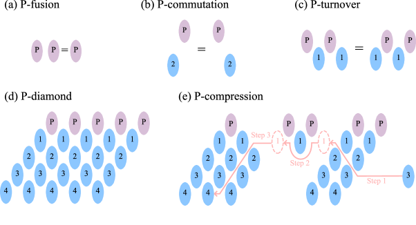
Figure 4: (a-c) P-block properties given in Def. 2. (d) The diamond structure defined in Def. 3 with height $n=4$. (e) Proof of Thm. 1, i.e. how the diamond can absorb a block. For this specific illustration, size of the diamond is $n=4$ and the index of the block is $i=3$. The block is lifted by other blocks via turnover, passes through the P-blocks via P-turnover, and then finally gets absorbed by other blocks via block properties.

This means that the TFIM and TFXY block mappings given in Eqs. 11 and 12 are capable of generating long-range quadratic terms, and can be used to compress quadratic fermionic Hamiltonians on any lattice of form Eq. 18. An illustration of this is given in Fig. 3 panel (a). Moreover, the fermionic swap gate allows us to move the fermion creation (annihilation) operator around as illustrated in Eq. 21. Therefore, leveraging the simple observation that the fermionic swap gate is a TFXY block, we are able to extend our compression method to the following Hamiltonian

$$\begin{split}\mathcal{H}(t)=\sum_{i,j}\big{(}&h_{ij}(t)\,c_{i}^{\dagger}c_{j}+p_{ij}(t)\,c_{i}c_{j}+q_{i}(t)\,c_{i}\big{)}+\text{h.c.},\end{split}$$ (25)

where $h_{ij}(t)$, $p_{ij}(t)$ and $q_{i}(t)$ are complex functions of time. Eq. 25 includes long-range hoppings and fermion creation (annihilation) on any site. Compressibility of Eq. 25 is illustrated in Fig. 3 panel (b).

IV Compression of Controlled Free Fermion Evolution

In this section, we extend our compression method by introducing a new object, called a $P$-block, that satisfies a new set of rules. We show that the combination of these new rules with the $B$-block rules given in Def. 1 leads to a compression algorithm applicable to any circuit that consists of $P$-blocks and $B$-blocks. The circuits are of a fixed depth that is independent of simulation time. We then show that evolution of a controlled free fermionic Hamiltonian can be mapped to this structure of $B$-blocks and $P$-blocks.

IV.1 $P$-Block Compression

We define a $P$-block as a mathematical object that satisfies the following relations.

Definition 2 ($P$-Block).

Given blocks $B_{i}$ with $i\geq 1$, define a “$P$-Block” $P=P(\bm{\theta})$ as a structure that satisfies

1. $P$-fusion: For any set of parameters $\bm{\alpha}$ and $\bm{\beta}$, there exist $\bm{a}$ such that

   $$P(\bm{\alpha})\,P(\bm{\beta})=P(\bm{a}),$$ (26)

2. $P$-commutation: For any set of parameters $\bm{\alpha}$ and $\bm{\beta}$

   $$P(\bm{\alpha})\,B_{i}(\bm{\beta})=B_{i}(\bm{\beta})\,P(\bm{\alpha}),\qquad i>1,$$ (27)

3. $P$-turnover: For any set of parameters $\bm{\alpha}$, $\bm{\beta}$, $\bm{\gamma}$ and $\bm{\theta}$ there exist $\bm{a}$, $\bm{b}$, $\bm{c}$ and $\bm{d}$ such that

   $$B_{1}(\bm{\alpha})\,P(\bm{\beta})\,B_{1}(\bm{\gamma})\,P(\bm{\theta})=P(\bm{a})\,B_{1}(\bm{b})\,P(\bm{c})\,B_{1}(\bm{d}).$$ (28)

If $P$ and blocks $B_{i}$ satisfy the properties listed above, we will say that $\{P,B_{i}\}$ is a $P$-block mapping.

These $P$-block properties are illustrated in Fig. 4 panels (a-c).

Let us define the following structure:

Definition 3 (Diamond).

Define a “diamond” with height $n$ as

$$D_{n}(\vec{\bm{\alpha}},\vec{\bm{\beta}}):=\prod_{m=1}^{n}\left[\left(\prod_{i=n\downarrow}^{1}B_{i}(\bm{\alpha}_{i,m})\right)P(\bm{\beta_{m}})\right]$$ (29)

where $B_{i}$ are blocks, $P$ is a P-block and each term in the product can have different variables.

An illustration of P-diamond with height 4 can be found in Fig. 4 panel (d). Now let us prove that this structure can absorb any block and P-block.

Theorem 1 ($P$-compression).

A diamond with height $n$ can be merged with any block $B_{i}$ with $i=1,2,...,n$ and P-block $P$:

$$\begin{split}&D_{n}(\vec{\bm{\alpha}},\vec{\bm{\beta}})\,P(\bm{\gamma})=D_{n}(\vec{\bm{a}},\vec{\bm{b}}),\\ &D_{n}(\vec{\bm{\alpha}},\vec{\bm{\beta}})B_{i}(\bm{\theta})=D_{n}(\vec{\bm{u}},\vec{\bm{v}}).\end{split}$$ (30)

Merging $P$ requires only one $P$-fusion. Merging $B_{i}$ requires $n-i-2$ turnovers, $1$ $P$-turnover and $1$ fusion.

Proof.

The proof of this results is given diagramatically in Fig. 4 panel (e). Since it is trivial to show that the diamond structure can absorb a $P$-block using the $P$-fusion operation, we only discuss how the diamond can absorb $B_{i}$. The illustration is for $n=4$ and $i=3$ case, but the same mechanism generalizes to arbitrary (finite) system sizes and $B_{i}$.

In step 1, the block $B_{i}$ gets shifted upwards through the diamond via normal block turnover operations until its index reaches $1$. Starting at index $i$ (which is 3 in the figure above), this upward movement requires $i-1$ turnover operations. In step 2 a $P$-turnover is applied, which brings the block from the right side to the left side of the formation of blocks shown in the middle of the figure above. Finally, in step 3, we can shift the block downward to the final row of blocks in the diamond. This again requires only normal block turnover operations, more precisely, we need $n-1$ turnover operations to move the block down to the bottom row of a $P$-diamond of height $n$ ($n=4$ in the figure above). At this stage, the block can then be fused with corresponding index $n$ block. This operation requires $n-i-2$ turnover operations, $1$ $P$-turnover operation and $1$ fusion operation in total. ∎

In the next section we discuss controlled free fermionic Hamiltonians as an example of a $P$-compressible Hamiltonian. However, we note that the theorem does not directly rely on the Hamiltonian, it only requires a set of circuit elements that follow the $B$-block and $P$-block rules. Thus, any circuit that is solely composed of gates that satisfy these rules can be compressed to a diamond, whether it is a controlled time evolution circuit of a free fermionic system or not.

IV.2 Controlled Free Fermions

Consider the following Hamiltonian representing a free fermion system coupled to an ancilla qubit with index 0,

$$\begin{split}\mathcal{H}_{\mathrm{full}}(t)&=\sum_{i,j}\big{(}u_{ij}(t)\,c_{i}^{\dagger}c_{j}+v_{ij}(t)\,c_{i}c_{j}+\text{h.c.}\big{)}\\ &+\sum_{i,j}\big{(}u^{\prime}_{ij}(t)\,Z_{0}c_{i}^{\dagger}c_{j}+v^{\prime}_{ij}(t)\,Z_{0}c_{i}c_{j}+\text{h.c.}\big{)}.\end{split}$$ (31)

This Hamiltonian applies a free fermionic evolution with hoppings $u_{ij}\pm u^{\prime}_{ij}$ and $v_{ij}\pm v^{\prime}_{ij}$ where the sign in between is $+$ if the ancilla is in $\ket{0}$ state, and $-$ if the ancilla is in $\ket{1}$ state.

This Hamiltonian is a generalization of a controlled free fermionic Hamiltonian version where the system remains the same if the ancilla is $\ket{0}$, and evolves if the ancilla is $\ket{1}$. To clarify, the controlled version of Eq. 18 can be represented via Eq. 31 with $u_{ij}=-u^{\prime}_{ij}=h_{ij}/2$ and $v_{ij}=-v^{\prime}_{ij}=p_{ij}/2$

By using (compressible) FSWAP gates as previously described in Sec. III.3, we can simply assume that all hoppings in a free fermionic Hamiltonian are nearest-neighbor. It directly follows that the time evolution of $\mathcal{H}_{\mathrm{full}}$ with the additional control generates the following controlled triangle structure,

(32)

where the top most qubit is the ancilla at index $0$, and the $Z_{0}$ attached blocks represent the quadratic terms in the second sum in Eq. 31.

In order to reduce the set of gates we need to consider to analyze the controlled triangle to a single new gate, we extend Eq. 23 to the controlled case,

$$Z_{0}c_{1}c_{4}=\mathcal{F}_{3,4}\mathcal{F}_{2,3}\ Z_{0}c_{1}c_{2}\ \mathcal{F}_{2,3}^{\dagger}\mathcal{F}_{3,4}^{\dagger},$$ (33)

which follows directly from Eq. 23 as the FSWAP gates do not act on the $0$th qubit and therefore commute with $Z_{0}$. Graphically, this equality looks like,

(34)

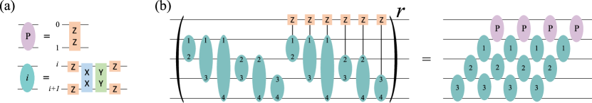
Figure 5: (a) The controlled TFXY P-block mapping given in Eq. 36. (b) Compression of the time evolution circuit of the Hamiltonian Eq. 31 into a diamond. For $n$ qubits, the number of CNOTs scales as $O(n^{2})$, and the depth scales as $O(n)$ up to a constant factor.

It follows from Eq. 33 that we only need to consider $Z_{0}c_{1}c_{2}$ which, in terms of blocks, corresponds to a controlled $B^{\mathrm{TFXY}}_{1}$ block. $B^{\mathrm{TFXY}}_{1}$ can be considered as the time evolution operator of a quadratic fermionic Hamiltonian on 2 sites. Therefore, it can be diagonalized via a combination of a Bogolyubov transformation and a basis transformation. The combined similarity transformation is just a TFXY block. In diagonal form, the Hamiltonian becomes $\epsilon_{1}\,c_{1}^{\dagger}c_{1}+\epsilon_{2}\,c_{2}^{\dagger}c_{2}$, which is a linear combination of $Z_{1}$ and $Z_{2}$. Therefore, $B^{\mathrm{TFXY}}_{1}$ is diagonalized via a $B^{\mathrm{TFXY}}_{1}$ rotation, and its diagonal part is a product of $Z_{1}$ and $Z_{2}$ rotations. In the case of a controlled $B^{\mathrm{TFXY}}_{1}$ block, only the diagonal part has to be controlled due to nature of a similarity transformation. It follows that a controlled $B^{\mathrm{TFXY}}_{1}$ block can be written as,

(35)

where, in the second equality, we have lifted the $Z_{2}$ rotation to a $Z_{1}$ rotation using a fermionic swap operation.

This shows that the only new gate we are adding to the TFXY block mapping is $P^{\mathrm{TFXY}}(\theta)=e^{i\theta Z_{0}Z_{1}}$. The $P^{\mathrm{TFXY}}(\theta)$ gate trivially satisfies the $P$-fusion and $P$-commutation rules. In Appendix D we show that this gate also satisfies the $P$-turnover property in combination with the TFXY block mapping. Therefore, $\{P^{\mathrm{TFXY}},B_{i}^{\mathrm{TFXY}}\}$ is a P-block mapping by Def. 2, and by Thm. 1 any circuit consisting of the gates given in the following mapping can be compressed into a diamond,

$$\begin{split}P^{\mathrm{TFXY}}(\theta)\equiv\ &e^{i\theta Z_{0}Z_{1}},\\ B^{\mathrm{TFXY}}_{i}(\bm{\theta})\equiv\ &e^{i\theta_{1}\>Z_{i}}e^{i\theta_{2}\>Z_{i+1}}e^{i\theta_{3}\>X_{i}X_{i+1}}\\ &e^{i\theta_{4}\>Y_{i}Y_{i+1}}\>e^{i\theta_{5}\>Z_{i}}e^{i\theta_{6}\>Z_{i+1}}.\end{split}$$ (36)

The mapping is illustrated in Fig. 5 panel (a).

We remark that the main advantage of the diamond structure is that it still only requires nearest-neighbor QPU connectivity compared to the all-to-one connectivity required for the controlled triangle we started from. If the circuit was to be implemented as given in Eq. 32, for all to all connected hardware the circuit would require 4 times as many CNOT gates compared to TFXY triangle. This is because a controlled TFXY block can be implemented as in the middle expression in Eq. 35, which has 2 TFXY blocks and 2 $ZZ$ gates, leading to 8 CNOTs for all to all connected topology. If the hardware has only a linear topology, the number of CNOTs gets to scale as $O(n^{3})$ compared to the $O(n^{2})$ scaling of the non-controlled case. The additional $n$ in the complexity comes from the fact that the ancilla need to reach to every qubit in the system. And finally, since everything is connected to the ancilla, none of these operations could be parallelized, leading to $O(n^{2})$ depth for all to all connectivity, and $O(n^{3})$ depth for the linear connectivity. For the linear topology, we will reduce the required number of CNOT gates to approximately 2 times of the TFXY triangle which scales as $O(n^{2})$, and the depth to the depth of the TFXY triangle which scales as $O(n)$.

V Results

V.1 Ground State Preparation of 1-D Free Fermions via Adiabatic State Preparation

We will be generating the ground state of the following Hamiltonian

$$\mathcal{H}_{0}=-\tilde{t}\sum_{i=1}^{n-1}\left(c^{\dagger}_{i}c^{\phantom{\dagger}}_{i+1}+c^{\dagger}_{i+1}c^{\phantom{\dagger}}_{i}\right)-\mu\sum_{i=1}^{n}c^{\dagger}_{i}c^{\phantom{\dagger}}_{i},$$ (37)

for $\tilde{t}=1$ and $\mu=0$. For large negative values of $\mu$, the chemical potential term will dominate and the ground state will be the empty state $\ket{000...0}$, which is easy to prepare. Thus, if we change $\mu$ sufficiently slowly, by the adiabatic theorem we can prepare the ground state of the Hamiltonian with $\mu=0$ as long as the energy gap between the ground state and the first excited state does not become zero. This method is called adiabatic state preparation (ASP).

ASP comes with competing challenges for the current noisy hardware. First, the Hamiltonian needs to be changed adiabatically — a small $d\mu/dt$ which requires a long evolution time $T$. At the same time, due to the Trotter decomposition, the time step $\delta t$ should be small. Altogether, this leads to a large number of Trotter steps $r=T/\delta t\gg 1$. For the non-compressable cases, it is difficult to simulate $r\gg 1$ due to hardware noise.

A second challenge for the adiabatic state preparation $\mathcal{H}_{0}$ ground state preparation comes from the symmetries of the Hamiltonian. The Hamiltonian Eq. 37 conserves particle number, which makes the adiabatic state preparation approach difficult. When $\mu=0$ the Hamiltonian Eq. 37 is particle-hole symmetric, and the ground state will be half filled. However, the initial state has no particles in it. Thus, without a symmetry breaking term, it is not possible to reach the ground state of $\mathcal{H}_{0}(\mu=0)$ since evolution under Eq. 37 does not change the particle number. More generally, the system has protected level crossings in the spectrum which makes the adiabatic state preparation impossible, unless an additional symmetry breaking term is added to the Hamiltonian to open gaps at those level crossing points.

In the TFXY model (which is equivalent to Eq. 37 after a Jordan-Wigner transformation), a global transverse $X$-direction magnetic field can generate gaps in the spectrum [40]. A global magnetic field is however not compressible; a field on the second site ($X_{2}=Z_{1}\big{(}c_{2}+c^{\dagger}_{2}\big{)}$) is cubic in fermion terms, which makes the dynamical Lie algebra grow exponentially with the system size. However, as we show above, a field on the first site ($c_{1}+c^{\dagger}_{1}=X_{1}$) is. Thus, we will add a single term that creates/annihilates particles on site 1

$$\mathcal{H}^{\prime}(t)=\lambda(t)\big{(}c_{1}+c^{\dagger}_{1}\big{)}$$ (38)

which in spin language corresponds to a local magnetic field in $X$ direction. This is sufficient to generate gaps between the ground state and the first excited state. Thus the addition of $\mathcal{H}^{\prime}$ addresses both of the challenges listed above: it opens up gaps by breaking the particle conservation symmetry, and its evolution together with $\mathcal{H}_{0}(\mu)$ is compressible into a circuit that is independent of the number of Trotter steps $r$ which needs to be large for ASP.

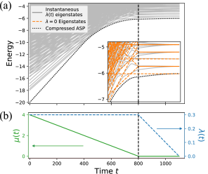
Figure 6: Adiabatic state preparation for the 1D chain via fermionic compression. (a) Instantaneous eigenstates and the result of the compressed time evolution with the parameters discussed in the text. Inset: a close-up view near the end of the evolution, with the instantaneous eigenvalues of $\mathcal{H}_{0}$ (orange dashed lines) and $\mathcal{H}=\mathcal{H}_{0}+\mathcal{H}^{\prime}$ (gray lines). (b) Time evolution of the chemical potential $\mu(t)$ and symmetry-breaking field $\lambda(t)$.

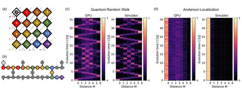
Figure 7: Simulation results from ibm_washington of a free-fermion on a two-dimensional (2D) lattice. (a) Schematic of the 16-site, 2D lattice, color-coded by the distance $M$ each lattice site is from the reference lattice site, labeled ‘0’. The fermion is initialized at reference lattice site ‘0’, and is allowed to evolve freely in time. (b) The topology of the qubits in the ibmq_washington quantum processing unit (QPU) is shown, along with how the lattice sites from the schematic in panel (a) are mapped to the particular 16 qubits used in these simulations. (c) The occupation number at each distance $M$ versus time with no disorder in the lattice. This leads to ballistic transport of the fermion. The left-hand plot shows results from the QPU, while the right-hand plot shows results from a noise-free quantum simulator. (d) The occupation number at each distance $M$ versus time with random disorder in the lattice. This leads to Anderson localization of the fermion. The left-hand plot shows results from the QPU, while the right-hand plot shows results from a noise-free quantum simulator.

Fig. 6 shows the results of adiabatic state preparation of the ground state of $\mathcal{H}_{0}$ for $N=10$ sites on a simulator. We initiate our state with no particles $\ket{\psi(t=0)}=\ket{000...0}$ with $\lambda(t=0)=0.3$ and $\mu(t=0)=-4$. The amplitude of the chemical potential is large enough to ensure that the $0-$particle state has large overlap with the ground state, even with non-zero $\lambda$. We evolve the state with $d\mu/dt=-0.005$ and constant $\lambda=0.3$ to keep the gaps open until we reach $\mu(t)=0$ at $t=800$. As a final step, we slowly turn off $\lambda$ with $d\lambda/dt=-0.001$ and $\mu=0$ until we reach $\lambda=0$ to obtain the true ground state of $\mathcal{H}_{0}$ in Eq. 37 at $\mu=0$.

As can be seen in Fig. 6, the energies obtained through adiabatic evolution compare well to the instantaneous ground state energies of $\mathcal{H}=\mathcal{H}_{0}+\mathcal{H}^{\prime}$ with $\lambda=0.3$. In the inset, it is clear that the ground and the first excited state $\mathcal{H}_{0}$ cross frequently — this is due to particle number conservation of $\mathcal{H}_{0}$. The nonzero $\lambda$ breaks the symmetry and opens up a gap at each of these level crossings between the ground and the first excited states. However, the gap is relatively small, therefore rate of change of $\mu$ must be small.

Satisfying the requirements of slow changes in the Hamiltonian, small $\delta t$, and a symmetry breaking field is enabled by the compression algorithm, which allows for arbitrarily long evolution at a fixed depth. Thus, both $\delta t$ and $d\mu/dt$ can be as small as desired in the Trotter expansion. As a simple first order Trotter circuit without compression, using $\delta t=0.4$ until $t=800$ and $\delta t=0.2$ for the remainder, this circuit consists of 3500 Trotter steps and 315,000 CNOTs. After compression, the circuit is structured as shown in Fig. 2 with 108 CNOTs.

V.2 2-D Fermionic Random Walk

In this example, we demonstrate how our compressed circuits can be used to simulate transport of free-fermions with long-range hopping [41]. In particular, we consider a fermion initialized on a reference lattice site, and observe how it evolves freely through a two-dimensional (2D) lattice. The lattice, pictured in Fig. 7a, comprises 16 sites with open boundary conditions. The lattice site labeled ’0’ is considered our reference site, where a fermion will be initialized. The lattice sites are color-coded by their distance $M$ to this reference site. Each lattice site is mapped to a qubit on the ibmq_washington quantum processing unit (QPU), which is one of the IBM Quantum Eagle r1 processors. While we assume only nearest-neighbor interactions between lattice sites, note that the 2D lattice of sites is mapped to a one-dimensional chain on the QPU, and thus requires long-range hopping operations. For example, in the 2D lattice, the fermion can hop between nearest-neighbor sites 11 and 15 (see Fig. 7a), but when the lattice is mapped to the qubits in the QPU, sites 11 and 15 are no longer neighbors (see Fig. 7b), and thus a long-range interaction between these qubits must be implemented. We examine transport of a fermion on this 16-site lattice both with and without disorder. To do this, we track the occupation number at varying distances $M$ from the reference site as the fermion evolves freely through time. When there is no disorder in the system, we expect the fermion to behave ballistically and oscillate back and forth within the lattice. Fig. 7c shows results from simulating a free fermion on a 2D lattice with no disorder on the ibmq_washington QPU as well as on a noise-free quantum simulator. The colors in the plots correspond to the occupation number at each distance $M$ versus evolution time. When there is large random disorder in the system, we expect the fermion to exhibit Anderson localization. Fig. 7d shows results from simulating a free fermion on a 2D lattice with large random disorder on the ibmq_washington QPU as well as on a noise-free quantum simulator. All simulations on the QPU were performed with 100,000 shots and any shot that did not conserve particle number was discarded. While results from the QPU are still noisy, a difference in transport can clearly be identified between lattices with and without disorder. We attribute the impressive results of these 16-qubit dynamic simulations on a real QPU to our compression algorithm, which produces short-depth circuits that do not grow with increasing evolution time.

VI Discussion and Outlook

With the developments in this paper, we have significantly extended the class of Hamiltonians whose evolution may be compressed. Specifically, any mean field Hamiltonian on an arbitrary lattice can now be simulated efficiently. In addition to that, currently we can add particles on a given mode with any amplitude. In [10] it was shown that for momentum conserving Hamiltonians, obtaining Green’s functions directly on the momentum basis via perturbing the system with $c^{\dagger}_{k}$ yields less noisy results compared to obtaining perturbing with $c^{\dagger}_{r}$ and post processing via Fourier transformation. For other systems such as chemistry examples, these single particle modes are more general, and can be obtained via our compression algorithm. With the addition of controlled evolution, these techniques are now applicable in a broader regime. Controlled evolution is a key step in quantum phase estimation, and similarly plays a role in computing Hamiltonian matrix elements for real time subspace expansions [42].

The compression algorithm discussed here is not limited to compressing time evolution. Rather, it may be applied to any set of quantum gates that obey the $B$-block and $P$-block properties. As long as the block mapping can be found, the algorithms developed here can be readily applied. We do not expect that general state preparation or other similar algorithms can be fully compressed as the compressed circuits lack expressibility; the states that can be reached are somewhat limited [20, 43]. However, there may be sizable subsets of the full quantum circuits whose elements do obey the block properties, and may be significantly shortened. We expect that the developments made in this work can thus have significant impact in transpiler software.

Appendix A Block Mapping for Long-Range Hoppings

Here we will show that we can build long-range fermion hopping and pair annihilation/creation operators using fermionic swap gates and TFXY blocks. We will define the fermionic swap operation as the following gate:

$$\mathcal{F}=\exp\left(i\frac{\pi}{2}\begin{bmatrix}1&0&0&0\\ 0&0&1&0\\ 0&1&0&0\\ 0&0&0&-1\end{bmatrix}\right).$$ (39)

Since the exponent matrix squares to identity,

$$\mathcal{F}=\cos\left(\frac{\pi}{2}\right)I_{4\times 4}+i\sin\left(\frac{\pi}{2}\right)\begin{bmatrix}1&0&0&0\\ 0&0&1&0\\ 0&1&0&0\\ 0&0&0&-1\end{bmatrix}=i\begin{bmatrix}1&0&0&0\\ 0&0&1&0\\ 0&1&0&0\\ 0&0&0&-1\end{bmatrix},$$ (40)

thus $\mathcal{F}$ is just a SWAP gate that keeps track of the fermionic sign up to a global phase. Calculating the Pauli string coefficients of the exponent yields

$$\begin{bmatrix}1&0&0&0\\ 0&0&1&0\\ 0&1&0&0\\ 0&0&0&-1\end{bmatrix}=\frac{1}{2}\begin{bmatrix}Z+I&X-iY\\ X+iY&Z-I\end{bmatrix}=\frac{1}{2}\big{(}XX+YY+IZ+ZI\big{)}.$$ (41)

where we use the notation $BA$ rather than $A_{1}B_{2}$ index notation for convenience. Combining with Eq. 39 and using $[XX+YY,IZ+ZI]=0$,

$$\begin{split}\mathcal{F}&=e^{i\frac{\pi}{4}(XX+YY+IZ+ZI)},\\ &=e^{i\frac{\pi}{4}(XX+YY)}e^{i\frac{\pi}{4}(IZ+ZI)},\\ &=e^{i\frac{\pi}{4}XX}e^{i\frac{\pi}{4}YY}e^{i\frac{\pi}{4}IZ}e^{i\frac{\pi}{4}ZI}.\end{split}$$ (42)

which is of TFXY block form as given in Eq. 12 with $\theta_{1}=\theta_{2}=0$ and $\theta_{3}=\theta_{4}=\theta_{5}=\theta_{6}=\pi/4$.

Now, let us check the effect $\mathcal{F}$ has on particle creation-annihilation operators:

$$\begin{split}\mathcal{F}\>IX\>\mathcal{F}^{\dagger}&=e^{i\frac{\pi}{4}XX}e^{i\frac{\pi}{4}YY}e^{i\frac{\pi}{4}ZI}e^{i\frac{\pi}{4}IZ}\ IX\ e^{-i\frac{\pi}{4}IZ}e^{-i\frac{\pi}{4}ZI}e^{-i\frac{\pi}{4}YY}e^{-i\frac{\pi}{4}XX},\\ &=e^{i\frac{\pi}{4}XX}e^{i\frac{\pi}{4}YY}e^{i\frac{\pi}{4}ZI}\ (-IY)\ e^{-i\frac{\pi}{4}ZI}e^{-i\frac{\pi}{4}YY}e^{-i\frac{\pi}{4}XX},\\ &=e^{i\frac{\pi}{4}XX}\ (-IY)\ e^{-i\frac{\pi}{4}XX},\\ &=XZ.\end{split}$$ (43)

Similarly for $IY$ we have that,

$$\begin{split}\mathcal{F}\>IY\>\mathcal{F}^{\dagger}&=e^{i\frac{\pi}{4}XX}e^{i\frac{\pi}{4}YY}e^{i\frac{\pi}{4}ZI}e^{i\frac{\pi}{4}IZ}\ IY\ e^{-i\frac{\pi}{4}IZ}e^{-i\frac{\pi}{4}ZI}e^{-i\frac{\pi}{4}YY}e^{-i\frac{\pi}{4}XX},\\ &=e^{i\frac{\pi}{4}XX}e^{i\frac{\pi}{4}YY}e^{i\frac{\pi}{4}ZI}\ IX\ e^{-i\frac{\pi}{4}ZI}e^{-i\frac{\pi}{4}YY}e^{-i\frac{\pi}{4}XX},\\ &=e^{i\frac{\pi}{4}YY}\ IX\ e^{-i\frac{\pi}{4}YY},\\ &=YZ.\end{split}$$ (44)

Considering the fact that,

$$\begin{split}\mathcal{F}^{2}&=e^{i\frac{\pi}{2}\big{(}XX+YY+IZ+ZI\big{)}},\\ &=e^{i\frac{\pi}{2}XX}e^{i\frac{\pi}{2}YY}e^{i\frac{\pi}{2}IZ}e^{i\frac{\pi}{2}ZI},\\ &=i^{4}\>XX\>.\>YY\>.\>IZ\>.\>ZI=-II.\end{split}$$ (45)

We can show that Eqs. 43 and 44 hold in the reverse direction as well,

$$\mathcal{F}\>XZ\>\mathcal{F}^{\dagger}=\mathcal{F}^{2}\>IX\>(\mathcal{F}^{2})^{\dagger}=(-II)\>IX\>(-II)=IX,$$ (46)

and

$$\mathcal{F}\>YZ\>\mathcal{F}^{\dagger}=\mathcal{F}^{2}\>IY\>(\mathcal{F}^{2})^{\dagger}=(-II)\>IY\>(-II)=IY.$$ (47)

Then we can show that after a Jordan-Wigner transformation,

$$c_{1} =\frac{1}{2}(IX-iIY), c_{2}=\frac{1}{2}(XZ-iYZ),$$

$$c_{1}^{\dagger} =\frac{1}{2}(IX+iIY), c_{2}^{\dagger}=\frac{1}{2}(XZ+iYZ),$$ (48)

we have that,

$$\mathcal{F}c_{1}\mathcal{F}^{\dagger} =c_{2}, \mathcal{F}c_{2}\mathcal{F}^{\dagger}=c_{1},$$

$$\mathcal{F}c_{1}^{\dagger}\mathcal{F}^{\dagger} =c_{2}^{\dagger}, \mathcal{F}c_{2}^{\dagger}\mathcal{F}^{\dagger}=c_{1}^{\dagger}.$$ (49)

In words, under a similarity transformation with $\mathcal{F}$, a creation (annihilation) operation on the first site is moved the the second site, and vice versa. Note that with this mapping, the computational basis states $\ket{0}$ and $\ket{1}$ correspond to the one and zero fermion states respectively, i.e., $\ket{0}$ corresponds to a site with one fermion, and $\ket{1}$ corresponds to an empty site.

We have assumed so far that $\mathcal{F}$ acts on qubits $1$ and $2$. Now, we will show that this holds in general for any nearest-neighbor sites. We denote $\mathcal{F}$ acting on qubits $i$ and $j$ as $\mathcal{F}_{ij}$. Using the Jordan-Wigner mapping,

$$\begin{split}c_{n}&=\frac{1}{2}Z_{1}Z_{2}...Z_{n-1}(X_{n}-iY_{n}),\\ c_{n}^{\dagger}&=\frac{1}{2}Z_{1}Z_{2}...Z_{n-1}(X_{n}+iY_{n}),\end{split}$$ (50)

we immediately see that the effect of $\mathcal{F}_{n,n+1}$ gate is similar to what we have obtained previously for sites $1$ and $2$,

$$\mathcal{F}_{n,n+1}\ c_{n}\ \mathcal{F}_{n,n+1}^{\dagger} =c_{n+1}, \mathcal{F}_{n,n+1}\ c_{n+1}\ \mathcal{F}_{n,n+1}^{\dagger}=c_{n},$$

$$\mathcal{F}_{n,n+1}\ c_{n}^{\dagger}\ \mathcal{F}_{n,n+1}^{\dagger} =c_{n+1}^{\dagger}, \mathcal{F}_{n,n+1}\ c_{n+1}^{\dagger}\ \mathcal{F}_{n,n+1}^{\dagger}=c_{n}^{\dagger}.$$ (51)

which is Eq. 20. By repeatedly applying this property, creation/annihilation operators on any site can be related to the ones in another site.

Here we have shown that fermionic swap $\mathcal{F}$ gate is a TFXY block, and that it allows us to carry the fermionic creation and annihilation operators between any pair of sites, leading to the compressibility of long-range hoppings give in Sec. III.3

Appendix B Block Mapping for Annihilation/Creation operators

Let us re-state the TFIM block mapping [1, 2]

$$\begin{split}B^{\mathrm{TFIM}}_{2i-1}(\theta)&=e^{i\theta Z_{i}},\\ B_{2i}^{\mathrm{TFIM}}(\theta)&=e^{i\theta X_{i}X_{i+1}}\end{split}$$ (52)

With FSWAP which can be represented via TFIM blocks, we have shown that this mapping covers any free fermionic Hamiltonian with quadratic terms. Now we will show that with the inclusion of $B^{\mathrm{TFIM}}_{0}(\theta)=\exp(i\theta X_{1})$, we can compress a free fermionic Hamiltonian with creation/annihilation terms as well. Since we have already proved in Ref. [1] that $B^{\mathrm{TFIM}}_{i}$ are blocks for $i>1$, we will only focus on the relations that $B^{\mathrm{TFIM}}_{0}$ should satisfy:

Fusion: Since $B^{\mathrm{TFIM}}_{0}(a)B^{\mathrm{TFIM}}_{0}(b)=B^{\mathrm{TFIM}}_{0}(a+b)$, fusion is satisfied.

Commutation: Since $B^{\mathrm{TFIM}}_{0}$ acts on qubit 1 only, it commutes with any $B^{\mathrm{TFIM}}_{i}$ for $i>2$. We also have $[B^{\mathrm{TFIM}}_{0},B^{\mathrm{TFIM}}_{2}]=0$ since $B^{\mathrm{TFIM}}_{2}(\theta)=\exp(i\theta X_{1}X_{2})$, and $[X_{1},X_{1}X_{2}]=0$. Thus, $B^{\mathrm{TFIM}}_{0}$ commutes with all $B^{\mathrm{TFIM}}_{i}$ with $i>2$.

Turnover: We are to prove

$$B^{\mathrm{TFIM}}_{1}B^{\mathrm{TFIM}}_{0}B^{\mathrm{TFIM}}_{1}=B^{\mathrm{TFIM}}_{0}B^{\mathrm{TFIM}}_{1}B^{\mathrm{TFIM}}_{0}.$$ (53)

The Lie algebra generated via the exponents $X_{1}$ and $Z_{1}$ is $\mathfrak{su}(2)$, and the equation above is the well known Euler decomposition of it. Since the $X$ and $Z$ directions can be chosen arbitrarily as long as they are orthogonal, any term in $SU(2)$ can be written as $R_{x}R_{z}R_{x}$ and/or $R_{z}R_{x}R_{z}$, which proves the turnover property.

Now, in fermion language, $B_{1}$ can be written as

$$B^{\mathrm{TFIM}}_{1}(\theta)=e^{i\theta(c_{1}+c_{1}^{\dagger})},$$ (54)

therefore we can create/destroy particles. If we want to do it with a phase rather than direct summation of creation and annihilation operators, we should use

$$\begin{split}e^{i\phi}c_{1}+e^{-i\phi}c_{1}^{\dagger}&=\cos\phi(c_{1}+c_{1}^{\dagger})+i\sin\phi(c_{1}-c_{1}^{\dagger})\\ &=\cos\phi X_{1}+\sin\phi Y_{1}\\ &=e^{-i\phi Z_{1}}X_{1}=e^{-i\frac{\phi}{2}Z_{1}}X_{1}e^{i\frac{\phi}{2}Z_{1}}\end{split}$$ (55)

Therefore a generic Hermitian linear combination of annihilation/creation operators at cite 1 can be written in terms of blocks as

$$\begin{split}e^{i\theta(e^{i\phi}c_{1}+e^{-i\phi}c_{1}^{\dagger})}&=e^{-i\frac{\phi}{2}Z_{1}}e^{i\theta X_{1}}e^{i\frac{\phi}{2}Z_{1}}\\ &=B^{\mathrm{TFIM}}_{2}\Big{(}-\frac{\phi}{2}\Big{)}B^{\mathrm{TFIM}}_{1}(\theta)B^{\mathrm{TFIM}}_{2}\Big{(}\frac{\phi}{2}\Big{)}\end{split}$$ (56)

Therefore that is compressible as well.

Applying Eq. 21 on Eq. 56, and defining $M_{n}=\prod_{k=n-1\downarrow}^{1}\mathcal{F}_{k,k+1}$ as a short notation, it is easy to create/annihilate fermions in a generic unitary way:

$$\begin{split}e^{i\theta(e^{i\phi}c_{n}+e^{-i\phi}c_{n}^{\dagger})}&=M_{n}\>e^{-i\frac{\phi}{2}Z_{1}}e^{i\theta X_{1}}e^{i\frac{\phi}{2}Z_{1}}M_{n}^{\dagger}\\ &=M_{n}B^{\mathrm{TFIM}}_{2}\Big{(}-\frac{\phi}{2}\Big{)}B^{\mathrm{TFIM}}_{1}(\theta)B^{\mathrm{TFIM}}_{2}\Big{(}\frac{\phi}{2}\Big{)}M_{n}^{\dagger}\end{split}$$ (57)

Now, fermionic swap gates are TFXY blocks, and as it was stated before, TFIM and TFXY mappings are equivalent. Therefore we conclude that creation/annihilation at any site can be compressed down to a TFIM triangle circuit structure. Thus, every term in the following Hamiltonian

$$\begin{split}\mathcal{H}(t)=\sum_{i,j}\big{(}&h_{ij}(t)c_{i}^{\dagger}c_{j}+p_{ij}(t)c_{i}c_{j}\\ &+q_{i}(t)c_{i}+\text{H.c.}\big{)}.\end{split}$$ (58)

can be represented via TFIM blocks, and can be compressed into a triangle.

As it was stated in the manuscript and in [1, 2], TFXY mapping has 2 times less CNOT compared to TFIM. After obtaining the TFIM representation of the time evolution circuit for Eq. 58, we can use

(59)

to transform groups of TFIM blocks in the circuit can be merged into TFXY blocks to reduce the CNOT count by half, and obtain the following triangle structure given in Fig. 2(a):

(60)

The depth can be reduced by transforming the TFIM triangle into a TFIM square via Theorem 2 [1] before switching to TFXY blocks. While the endproduct is already shown in Fig. 2(b), the following illustrates how to obtain it for 5 qubits:

(61)

where U gates are generic one qubit rotations arising from the left out $B^{\mathrm{TFIM}}_{0}B^{\mathrm{TFIM}}_{1}B^{\mathrm{TFIM}}_{0}=R_{x}R_{z}R_{x}$ on the top line.

Appendix C Fermion Creation with Definite Momentum

One of the interesting features we can exploit from the compressibility of Eq. 25 is that it allows us to create particles in any single particle mode. Here we will specifically show how to generate a circuit that creates a particle with a definite momentum $k$.

Creation operators in momentum space $c^{\dagger}_{k}$ are a discrete Fourier transformation of creation operators in position space $c^{\dagger}_{r}$:

$$c^{\dagger}_{k}=\sum_{r=1}^{n}e^{2\pi ikr/n}c^{\dagger}_{r},$$ (62)

where $k=0,1,2,...,n-1$ and $n$ is the number of lattice sites. The $c_{k}$ satisfy the anti-commutation relations $\{c_{p},c_{k}\}=\{c_{p}^{\dagger},c_{k}^{\dagger}\}=0$ and $\{c_{p},c_{k}^{\dagger}\}=\delta_{pq}$ where $\delta_{pq}$ is the Kronecker delta.

The state we would like to create is $\ket{\psi_{k}}=c^{\dagger}_{k}\ket{0}$ where $\ket{0}$ represents the empty fermion state, which is $\ket{000...0}$ in the computational basis. Unfortunately $c_{k}^{\dagger}$ is not a unitary operator. However, $c^{\dagger}_{k}+c^{\phantom{\dagger}}_{k}$ is Hermitian and due to the anti-commutation relations, we have $\big{(}c^{\dagger}_{k}+c^{\phantom{\dagger}}_{k}\big{)}^{2}=1$. Moreover, $c_{k}\ket{0}=0$. Combining these, we have

$$e^{i\theta\big{(}c^{\dagger}_{k}+c^{\phantom{\dagger}}_{k}\big{)}}\ket{0}=\cos(\theta)\ket{0}+i\sin(\theta)\big{(}c^{\dagger}_{k}+c^{\phantom{\dagger}}_{k}\big{)}\ket{0}=\cos(\theta)\ket{0}+i\sin(\theta)\ket{\psi_{k}}.$$ (63)

For $\theta=\pi/2$, we obtain $\psi_{k}$ up to a global phase

$$e^{i\frac{\pi}{2}\big{(}c^{\dagger}_{k}+c^{\phantom{\dagger}}_{k}\big{)}}\ket{0}=i\ket{\psi_{k}}.$$ (64)

Thus, if we implement time evolution unitary under $\mathcal{H}_{k}=c^{\dagger}_{k}+c^{\phantom{\dagger}}_{k}$ for time $t=-\pi/2$, we can create a particle with momentum $k$. Now, this Hamiltonian is a special case for the Hamiltonian in Eq. 25, and therefore we can generate a circuit via Trotter decomposition and compress it into a fixed depth circuit.

This method is not limited to creating a single particle. One can use the same unitary with different momentum $p$ to add another particle. Because $\ket{\psi_{k}}$ does not contain any particle with momentum $p\neq k$, $c_{p}\ket{\psi_{k}}=0$ still holds, and we can obtain

$$e^{i\frac{\pi}{2}\big{(}c^{\dagger}_{p}+c^{\phantom{\dagger}}_{p}\big{)}}e^{i\frac{\pi}{2}\big{(}c^{\dagger}_{k}+c^{\phantom{\dagger}}_{k}\big{)}}\ket{0}=ie^{i\frac{\pi}{2}\big{(}c^{\dagger}_{p}+c^{\phantom{\dagger}}_{p}\big{)}}\ket{\psi_{k}}=-\big{(}c^{\dagger}_{p}+c^{\phantom{\dagger}}_{p}\big{)}\ket{\psi_{k}}=-c^{\dagger}_{p}\ket{\psi_{k}}=-c^{\dagger}_{p}\>c^{\dagger}_{k}\ket{0}.$$ (65)

This corresponds to first evolving under $\mathcal{H}_{k}=c^{\dagger}_{k}+c^{\phantom{\dagger}}_{k}$, then under $\mathcal{H}_{p}=c^{\dagger}_{p}+c^{\phantom{\dagger}}_{p}$. This is still a special case of one evolution under the Hamiltonian Eq. 25 since the coefficient in Eq. 25 are time dependent. Switching from $\mathcal{H}_{k}$ to $\mathcal{H}_{p}$ is just changing coefficients via simulation time. This can be applied for different creating more particles with different momenta as well. Thus we can create any number of particles with different momenta via using the compression of Eq. 25.

As a remark, this is not limited to creating momentum definite states. This can be done for any orthonormal single particle basis simply by changing the coefficients of Eq. 62.

Appendix D Proof of $P$-block rules for $P^{\mathrm{TFXY}}(\theta)=\exp(i\theta Z_{0}Z_{1})$

In the manuscript, we have claimed that the mapping given in Eq. 12 is a P-set, and therefore can be compressed down to a diamond defined in Def. 3. Here we will prove that $P^{\mathrm{TFXY}}(\theta)=e^{i\theta Z_{0}Z_{1}}$ satisfy P-block rules.

Fusion: P-fusion is trivially satisfied since $P^{\mathrm{TFXY}}(a)P^{\mathrm{TFXY}}(b)=P^{\mathrm{TFXY}}(a+b)$.

Commutation: P-commutation is satisfied because $P^{\mathrm{TFXY}}$ only acts on qubits 0 and 1 whereas $B^{\mathrm{TFXY}}_{i}$ with $i\geq 2$ does not. The only remaining property is then P-turnover.

Turnover: To prove the P-turnover property, we will show that $B^{\mathrm{TFXY}}_{1}P^{\mathrm{TFXY}}B^{\mathrm{TFXY}}_{1}P^{\mathrm{TFXY}}$ can absorb $B^{\mathrm{TFXY}}_{1}$ and $P^{\mathrm{TFXY}}$ from right. To do so, let us switch to TFIM blocks via Eq. 14

(66)

In the second equality, we have used the fact that $Y$ can be obtained via rotating $X$ on the $Z$ axis, and in the last one we have used the triangle compression theorem for TFIM blocks. Also we have omitted the indices for convenience.

In addition, we have ommitted block indices for simplicity, and there are no qubit lines in the block representation because some blocks are 1 qubit gates and some are two qubit gates. If we represent $Z_{0}Z_{1}$ rotation gate as a dark TFIM block, we then will have

(67)

Observe that $Z_{0}Z_{1}$ commutes with $Z_{1}$, therefore $[P^{\mathrm{TFXY}},B^{\mathrm{TFIM}}_{1}]=0$ ((a) in the figure below). In addition, $Z_{0}Z_{1}$ and $X_{1}X_{2}$ generate a representation of $\mathfrak{su}(2)$, therefore by Euler decomposition, they satisfy a mixed kind of turnover property: $P^{\mathrm{TFXY}}B^{\mathrm{TFIM}}_{2}P^{\mathrm{TFXY}}=B^{\mathrm{TFIM}}_{2}P^{\mathrm{TFXY}}B^{\mathrm{TFIM}}_{2}$ ((b) in the figure below). And finally, we see that $P^{\mathrm{TFXY}}$ and $B^{\mathrm{TFIM}}_{3}$ act on different qubits, therefore they commute ((c) in the figure below). These properties can be illustrated as the following:

Figure S1: Relations $Z_{0}Z_{1}$ rotation gate satisfy with $B^{\mathrm{TFIM}}_{i}$ for $i=1,2,3$.

Using these relations and TFIM block relations, we can simplify Eq. 67:

(68)

Now we shall prove that this structure is capable of absorbing $P^{\mathrm{TFXY}}$ and $B_{1}^{\mathrm{TFXY}}$ (or rather $B_{1}^{\mathrm{TFIM}}$, $B_{2}^{\mathrm{TFIM}}$ and $B_{3}^{\mathrm{TFIM}}$).

(69)

The $P^{\mathrm{TFXY}}$ absorption is trivial, the new $P^{\mathrm{TFXY}}$ just merges to the right most $P^{\mathrm{TFXY}}$. $B_{1}^{\mathrm{TFIM}}$ absorption has 2 steps: it first commutes with $P^{\mathrm{TFXY}}$, and then gets absorbed via TFIM block rules. $B_{3}^{\mathrm{TFIM}}$ absorption has 3 steps: it first gets lifted via TFIM turnovers, commutes with $P^{\mathrm{TFXY}}$, and then gets absorbed via TFIM block rules. The more complex operation is the $B_{2}^{\mathrm{TFIM}}$ absorption: it gets lifted and becomes $P^{\mathrm{TFXY}}$ via the mixed turnover rule first. Then it commutes with $B_{1}^{\mathrm{TFIM}}$, pushed down via mixed turnover to be $B_{2}^{\mathrm{TFIM}}$ again and then gets absorbed via TFIM block rules.

Now that we have proved that $B^{\mathrm{TFXY}}_{1}P^{\mathrm{TFXY}}B^{\mathrm{TFXY}}_{1}P^{\mathrm{TFXY}}$ can absorb $P^{\mathrm{TFXY}}$ and $B^{\mathrm{TFXY}}_{1}$, consider the other ordering: $P^{\mathrm{TFXY}}B^{\mathrm{TFXY}}_{1}P^{\mathrm{TFXY}}B^{\mathrm{TFXY}}_{1}$. This expression consists of $P^{\mathrm{TFXY}}$ and $B^{\mathrm{TFXY}}_{1}$, therefore can be transformed into the form given in Eq. 68 by following the steps given in Eq. 69. Thus we have proven

(70)

The other direction can also be proven simply by inverting all the figures. It can be done since the TFIM block rules and mixed rules are symmetric under reflection. Therefore, we have proven that $P^{\mathrm{TFXY}}(\theta)=\exp(i\theta Z_{0}Z_{1})$ is a P-block for TFXY block mapping.