Distributionally Robust Optimization using Cost-Aware Ambiguity Sets

Abstract

We present a novel frameworkfor distributionally robust optimization (DRO),called cost-aware DRO (Cadro).The key idea of Cadro is to exploit the cost structurein the design of the ambiguity set to reduce conservatism.Particularly, the set specifically constrains theworst-case distributionalong the direction in which theexpected cost of an approximate solutionincreases most rapidly.We prove that Cadro provides both a high-confidenceupper bound and a consistent estimator of the out-of-sample expected cost, andshow empirically that it produces solutions that aresubstantially less conservative than existing DRO methods,while providing the same guarantees.

I Introduction

We consider the stochastic programming problem

$$\operatorname*{minimize}_{x\in X}\operatorname{{\rm I\mathchoice{}{}{}{}E}}[\ell(x,\xi)]$$ (1)

with $X\subseteq\Re^{n}$ a nonempty, closed set of feasible decision variables,$\xi\in\Xi$ a random variable following probability measure $\prob$,and $\ell:\Re^{n}\times\Xi\to\Re$ a known cost function.This problem is foundational in many fields, includingoperations research [shapiro_LecturesStochasticProgramming_2021],machine learning [hastie_ElementsStatisticalLearning_2009],and control (e.g., stochastic model predictive control) [mesbah_StochasticModelPredictive_2016].Provided that the underlying probability measure $\prob$ is known exactly,this problem can effectively be solved using traditionalstochastic optimization methods [royset_OptimizationPrimer_2021, shapiro_LecturesStochasticProgramming_2021].In reality, however, only a data-driven estimate $\hat{\prob}$ of $\prob$ istypically available, which may be subject to misestimations—known as ambiguity.Perhaps the most obvious method for handling this issue is to disregard thisambiguity and instead apply a sample average approximation (SAA) (also known as empirical risk minimization (ERM) in the machine learning literature), where(1) is solved using $\hat{\prob}$ as a plug-inreplacement for $\prob$.However, this is known to produce overly optimistic estimates ofthe optimal cost[royset_OptimizationPrimer_2021, Prop. 8.1],potentially resulting in unexpectedly high realizations of thecost when deploying the obtained optimizers on new, unseen samples.This downward bias of SAA is closely related to the issue of overfitting,and commonly refered to as the optimizer’s curse[smith_OptimizerCurseSkepticism_2006a, vanparys_DataDecisionsDistributionally_2021].Several methods have been devised over the years to combat this undesirable behavior.Classical techniques such as regularization and cross-validation arecommonly used in machine learning [hastie_ElementsStatisticalLearning_2009],although typically, they are used as heuristics, providing few rigorous guarantees,in particular for small sample sizes.Alternatively, the suboptimality gap of the SAA solution may be statistically estimatedby reserving a fraction of the dataset for independent replications [bayraksan_AssessingSolutionQuality_2006].However, these results are typically based on asymptotic arguments,and are therefore notvalid in the low-sample regime. Furthermore, although this type of approachmay be used to validate the SAA solution,it does not attempt to improve it, by taking into accountpossible estimation errors.More recently, distributionally robust optimization (DRO) has garnered considerable attention,as it provides a principled way of obtaining ahigh-confidence upper bound on the true out-of-sample cost [delage_DistributionallyRobustOptimization_2010, mohajerinesfahani_DatadrivenDistributionallyRobust_2018, vanparys_DataDecisionsDistributionally_2021].In particular, its capabilities to providerigorous performance and safety guarantees hasmade it an attractivetechnique for data-driven and learning-basedcontrol [hakobyan_DistributionallyRobustRisk_2022, schuurmans_SafeLearningbasedMPC_2023, tac2023].DRO refers to a broad class of methods in whicha variant of (1) is solvedwhere $\prob$ is replaced with a worst-case distribution withina statistically estimated set of distributions, called an ambiguity set.As the theory essentially requires only that the ambiguity setcontains the true distribution with a prescribed level of confidence,a substantial amount of freedom is left in the design of the geometry ofthese sets. As a result, manydifferent classes of ambiguity sets have beenproposed in the literature, e.g.,Wasserstein ambiguity sets [mohajerinesfahani_DatadrivenDistributionallyRobust_2018],divergence-based ambiguity sets [tac2023, vanparys_DataDecisionsDistributionally_2021, bayraksan_DataDrivenStochasticProgramming_2015]and moment-based ambiguity sets [delage_DistributionallyRobustOptimization_2010, coppens_DatadrivenDistributionallyRobust_2020];See [rahimian_FrameworksResultsDistributionally_2022, lin_DistributionallyRobustOptimization_2022]for recent surveys.Despite the large variety of existing classes of ambiguity sets,a common characteristic is that their design isconsidered separately from the optimization problem in question.Although this simplifies the analysis in some cases,it may also induce a significant level of conservatism;In reality, we are only interested in excluding distributions from theambiguity set which actively contribute to increasing the worst-case cost.Requiring that the true distribution deviates little from the data-driven estimatein all directions may therefore be unnecessarily restrictive.This intuition motivates the introduction of a new DRO methodology, which is aimedat designing the geometry of the ambiguity sets with the original problem (1)in mind. The main idea is that by only excluding those distributions that maximally affectthe worst-case cost, higher levels of confidence can be attained withoutintroducing additional conservatism to the cost estimate.

Contributions

1 We propose a novel class of ambiguity setsfor DRO,taking into account the structure of the underlying optimization problem; 2 We prove that the DRO cost is both a high-confidence upper boundand a consistent estimate of the optimal cost of the original stochastic program (1); 3 We demonstrate empirically that the provided ambiguity set outperforms existing alternatives.

Notation

We denote$[n]=\{1,\dots,n\},$for $n\in\N$.$|S|$ denotes the cardinality of a (finite) set $S$.$\e_{i}\in\Re^{n}$ is the $i$th standard basis vector in$\Re^{n}$. Its dimension $n$ will be clear from context.We denote the level sets of a function $f:\Re^{n}\to\Re$ as$\operatorname{lev}_{\leq\alpha}f\dfn\{x\in\Re^{n}\mid f(x)\leq\alpha\}$.We write ‘$\as$’ to signify that a random event occurs almost surely, i.e., with probability 1.We denote the largest and smallest entries of a vector $v\in\Re^{n}$as $v_{\mathrm{max}}\dfn\max_{i\in[n]}v_{i}$ and $v_{\mathrm{min}}=\min_{i\in[n]}v_{i}$,respectively, and define its range as$\operatorname{rg}(v)\dfn v_{\mathrm{max}}-v_{\mathrm{min}}.$$\delta_{X}$ is the indicator of a set $X$: $\delta_{X}(x)=0$ if $x\in X$,$+\infty$ otherwise.

II Problem Statement

We will assume that the random variable $\xi$ is finitely supported,so thatwithout loss of generality, we may write$\Xi=\{1,\dots,\nModes\}$.This allows us to define the probability mass vector$p=(\prob[\xi=i])_{i=1}^{\nModes},$and enumerate the cost realizations $\ell_{i}=\ell(\hskip 1.00006pt\mathbf{\cdot}\hskip 1.00006pt,i)$, $i\in[\nModes]$.Furthermore, it will be convenient to introduce the mapping$L:\Re^{n}\to\Re^{\nModes}$as$L(x)=(\ell_{1}(x),\dots,\ell_{\nModes}(x)).$We will pose the following (mostly standard) regularity assumption on the cost function.

Assumption II.1 (Problem regularity).

For all $i\in[\nModes]$

1. $\ell_{i}$ is continuous on $X$;

2. $\overline{\ell}_{i}\dfn\ell_{i}+\delta_{X}$ is level-bounded;

Since any continuous function is lsc (lsc),Assumption II.1 combined with the closedness of $X$ impliesinf-compactness, which ensures attainment of the minimum [rockafellar_VariationalAnalysis_1998, Thm. 1.9].Continuity of $\ell_{i}$ is used mainlyin LABEL:lem:parametric-stabilityto establish continuity of thesolution mapping $V^{\!\star}$—defined below, see (2).However, a similar result can be obtained by replacing condition (i)by lower semicontinuity and uniform level-boundedness on $X$.However, for ease of exposition, we will not cover this modification explicitly.Let $p^{\star}\in\Delta_{\nModes}\dfn\{p\in\Re^{\nModes}_{+}\mid{\textstyle\sum}_{i=1}^{\nModes}p_{i}=1\}$denote the true-but-unknown probability mass vector, anddefine$V:\Re^{n}\times\Delta_{\nModes}\to\Re:(x,p)\mapsto\langle p,L(x)\rangle$,to obtain the parametric optimization problem with optimal cost and solution set

$$V^{\!\star}(p)=\min_{x\in X}V(x,p)\text{ and }X^{\!\star}(p)=\operatorname*{\arg\!\min}_{x\in X}V(x,p).$$ (2)

The solution of (1) is retrieved by solving (2) with $p=p^{\star}$.Assume we have access toa dataset $\hat{\Xi}\dfn\{\xi_{1},\dots,\xi_{m}\}\in\Xi^{m}$collected i.i.d. from $p^{\star}$.In order to avoid the aforementioneddownward bias of SAA,our goal is to obtain adata-driven decision $\hat{x}_{m}$ along with an estimate$\hat{V}_{m}$ such that

$$\prob[V(\hat{x}_{m},p^{\star})\leq\hat{V}_{m}]\geq 1-\beta,$$ (3)

where $\beta\in(0,1)$ is a user-specified confidence level.We address this problem by means of distributionally robust optimization,where instead of (2), one solves the surrogate problem

$$\hat{V}_{m}=\min_{x\in X}\max_{p\in\mathcal{A}_{m}}V(x,p).$$ (DRO)

Here, $\mathcal{A}_{m}\subseteq\Delta_{\nModes}$ is a (typically data-dependent, and thus, random) set ofprobability distributions that is designed to contain the true distribution $p^{\star}$ withprobability $1-\beta$, ensuring that (3) holds.Trivially, (3) is satisfied with $\beta=0$ by taking $\mathcal{A}_{m}\equiv\Delta_{\nModes}$.This recovers a robust optimization method, i.e., $\min_{x\in X}\max_{i\in[\nModes]}\ell_{i}(x)$.Although it satisfies (3), this robust approach tends to be overly conservativeas it neglects all available statistical data.The aim of distributionally robust optimization is to additionally ensurethat $\hat{V}_{m}$ is a consistent estimator, i.e.,

$$\lim_{m\to\infty}\hat{V}_{m}=V^{\!\star}(p^{\star}),\quad\as.$$ (4)

We will say that a class of ambiguity sets is admissible if thesolution $\hat{V}_{m}$ of the resulting DRO problem (DRO)satisfies (3) and (4).Our objectiveis to develop a methodology forconstructing admissible ambiguity sets that take into account thestructure of (DRO) and in doing so, providetighter estimates of the cost, while maintaining (3) witha given confidence level $\beta$.

III Cost-Aware DRO

In this section, we describe the proposed DROframework, which we will refer to as cost-aware DRO (Cadro).The overall method is summarized in LABEL:alg:cadro.

III-A Motivation

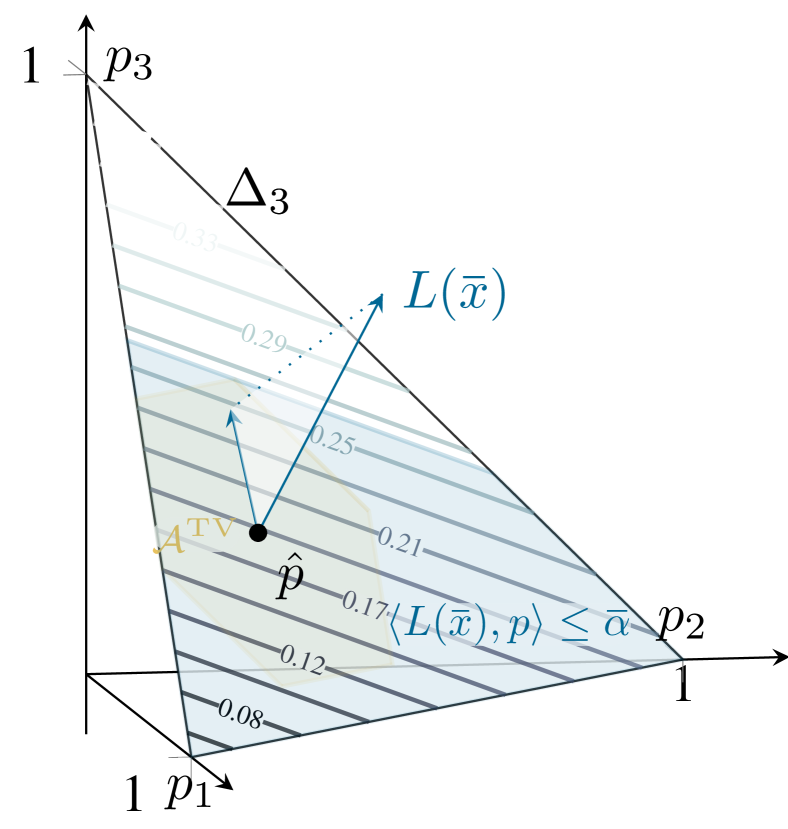
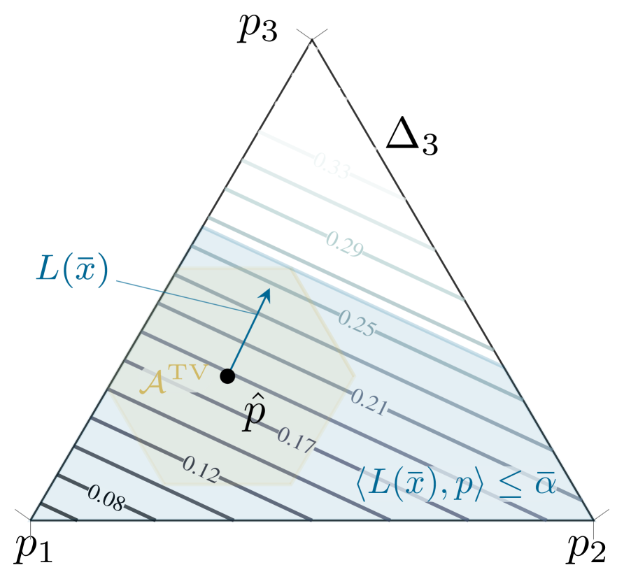
Figure 1: Conceptual motivation for the structure of theambiguity set (6).The cost contour lines$\{p\in\Delta_{3}\mid\langle L(\mkern 1.5mu\overline{\mkern-1.5mux\mkern-1.5mu}\mkern 1.5mu),p\rangle=\alpha\}$ corresponding tosome $\mkern 1.5mu\overline{\mkern-1.5mux\mkern-1.5mu}\mkern 1.5mu\in X$ are shown for increasing values of $\alpha$ (dark to light),together with the sets $\mathcal{A}^{\scriptscriptstyle\mathrm{TV}}\dfn\Delta_{3}\cap\ball_{1}(\hat{p},\varrho)$and $\mathcal{A}\dfn\{p\in\Delta_{3}\mid\langle L(\mkern 1.5mu\overline{\mkern-1.5mux\mkern-1.5mu}\mkern 1.5mu),p\rangle\leq\mkern 1.5mu\overline{\mkern-1.5mu\alpha\mkern-1.5mu}\mkern 1.5mu\}$.Here, $\varrho>0$ is determined to satisfy (5)and $\mkern 1.5mu\overline{\mkern-1.5mu\alpha\mkern-1.5mu}\mkern 1.5mu=\max_{p\in\mathcal{A}^{\scriptscriptstyle\mathrm{TV}}}\langle L(\mkern 1.5mu\overline{\mkern-1.5mux\mkern-1.5mu}\mkern 1.5mu),p\rangle$.Since $\mathcal{A}^{\scriptscriptstyle\mathrm{TV}}\subset\mathcal{A}$, $\mathcal{A}$ satisfies (5)with a higher confidence level $1-\beta$, but nevertheless, we have$\max_{p\in\mathcal{A}}V(\mkern 1.5mu\overline{\mkern-1.5mux\mkern-1.5mu}\mkern 1.5mu,p)=\max_{p\in\mathcal{A}^{\scriptscriptstyle\mathrm{TV}}}V(\mkern 1.5mu\overline{\mkern-1.5mux\mkern-1.5mu}\mkern 1.5mu,p)$.

We start by providing some intuitive motivation.Consider the problem (DRO).In order to provide a guarantee of the form(3),it obviously suffices to design $\mathcal{A}_{m}$such that

$$\prob[p^{\star}\in\mathcal{A}_{m}]\geq 1-\beta.$$ (5)

However, this condition alone still leavesa considerable amount of freedom to the designer.A common approach is to select$\mathcal{A}_{m}$ to be a ball (expressed in somestatistical metric/divergence)around an empiricalestimate $\hat{p}$ of the distribution.Depending on the choice of metric/divergence(e.g., total variation [rahimian_IdentifyingEffectiveScenarios_2019],Kullback-Leibler [vanparys_DataDecisionsDistributionally_2021],Wasserstein [mohajerinesfahani_DatadrivenDistributionallyRobust_2018], …),several possible variants may be obtained.Using concentration inequalities,one can then select the appropriate radius of this ball,such that (5) is satisfied.A drawback of this approach, however,is that the construction of $\mathcal{A}_{m}$ isdecoupled from the original problem (1).Indeed, given that $\mathcal{A}_{m}$ takes the form of a ball,(5) essentially requires the deviationof $\hat{p}$ from $p^{\star}$ to be small along every direction.If one could instead enlarge the ambiguity setwithout increasing the worst-case cost, then (5)could be guaranteed for smaller values of $\beta$ withoutintroducing additional conservatism.This idea is illustrated in Fig. 1.Conversely, for a fixed confidence level $\beta$,one could thus construct a smaller upper bound $\hat{V}_{m}$,by restricting the choice of $p$ only in a judiciously selected direction.Particularly, we may set$\mathcal{A}_{m}=\{p\in\Delta_{\nModes}\mid\langle L(\mkern 1.5mu\overline{\mkern-1.5mux\mkern-1.5mu}\mkern 1.5mu),p\rangle\leq\alpha_{m}\}$for some candidate solution $\mkern 1.5mu\overline{\mkern-1.5mux\mkern-1.5mu}\mkern 1.5mu\in X$,where $\alpha_{m}$ is the smallest (potentially data-dependent) quantitysatisfying (5).This directly yields an upper bound on the estimate$\hat{V}_{m}$. Namely,for $x^{\star}\in X^{\!\star}(p^{\star})$,we have with probability $1-\beta$,

$$V(x^{\star},p^{\star}) \stackrel{{\scriptstyle\hypertarget{a}{(a)}}}{{\leq}}V(\hat{x}_{m},p^{\star})\leq\max_{p\in\mathcal{A}_{m}}V(\hat{x}_{m},p)=\hat{V}_{m}$$

$$=\min_{x\in X}\max_{p\in\mathcal{A}_{m}}V(x,p)\stackrel{{\scriptstyle\hypertarget{b}{(b)}}}{{\leq}}\max_{p\in\mathcal{A}_{m}}V(\mkern 1.5mu\overline{\mkern-1.5mux\mkern-1.5mu}\mkern 1.5mu,p)=\alpha_{m}.$$

Here, inequalities (a) and (b)become equalities when $\hat{x}_{m}=x^{\star}=\mkern 1.5mu\overline{\mkern-1.5mux\mkern-1.5mu}\mkern 1.5mu$.Thus, a reasonable aim would be to select $\mkern 1.5mu\overline{\mkern-1.5mux\mkern-1.5mu}\mkern 1.5mu$to be a good approximation of $x^{\star}$.We will return to the matter of selecting $\mkern 1.5mu\overline{\mkern-1.5mux\mkern-1.5mu}\mkern 1.5mu$ in Section III-C.First, however,we will assume $\mkern 1.5mu\overline{\mkern-1.5mux\mkern-1.5mu}\mkern 1.5mu$ to be given and focus onestablishing the coverage condition (5).

III-B Ambiguity set parameterization and coverage

Motivated by the previous discussion,we propose a family of ambiguity sets parameterizedas follows.Let $v\in\Re^{\nModes}$ be a fixed vector(we will discuss the choice of $v$ in Section III-C).Given a sample $\hat{\Xi}=\{\xi_{1},\dots,\xi_{m}\}$ of size $|\hat{\Xi}|=m$drawn i.i.d. from $p^{\star}$,we consider ambiguity sets of the form

$$\mathcal{A}_{\hat{\Xi}}(v)\dfn\{p\in\Delta_{\nModes}\mid\langle p,v\rangle\leq\alpha_{\hat{\Xi}}(v)\},$$ (6)

where $\alpha:\Xi^{m}\times\Re^{\nModes}\ni(\hat{\Xi},v)\mapsto\alpha_{\hat{\Xi}}(v)\in\Re$is a data-driven estimator for $\langle p^{\star},v\rangle$,selected to satisfy the following assumption,which implies that (5) holdsfor $\mathcal{A}_{m}=\mathcal{A}_{\hat{\Xi}}(v)$.

Assumption III.1.

$\prob[\langle p^{\star},v\rangle\leq\alpha_{\hat{\Xi}}(v)]\geq 1-\beta,\;\forall v\in\Re^{\nModes}.$

Note that the task of selecting $\alpha$ to satisfy Assumption III.1is equivalent to findinga high-confidence upper bound on the mean of the scalar random variable$\langle v,\e_{\xi}\rangle$, $\xi\sim p^{\star}$.It is straightforward to derivesuch bounds by bounding thedeviation of a random variable from its empirical meanusing classical concentration inequalities like Hoeffding’s inequality.

Proposition III.2 (Hoeffding bound).

Fix $v\in\Re^{\nModes}$ and let$\hat{\Xi}$ with $|\hat{\Xi}|=m$, be an i.i.d. sample from $p^{\star}\in\Delta_{\nModes}$,with empirical distribution$\hat{p}_{{\scriptscriptstyle\hat{\Xi}}}=\tfrac{1}{m}{\textstyle\sum}_{\xi\in\hat{\Xi}}\e_{\xi}$.Consider the bound

$$\alpha_{\hat{\Xi}}(v)=\langle v,\hat{p}_{{\scriptscriptstyle\hat{\Xi}}}\rangle+r_{m}\operatorname{rg}(v).$$ (7)

This bound satisfies Assumption III.1, if $r_{m}$ satisfies

$$r_{m}=\min\big{\{}1,\sqrt{\tfrac{\log(\nicefrac{{1}}{{\beta}})}{2m}}\big{\}}.$$ (8)

Proof.

Define$y_{k}\dfn\langle p^{\star}-\e_{\xi_{k}},v\rangle,$so that $\tfrac{1}{m}{\textstyle\sum}_{k=1}^{m}y_{k}=\langle p^{\star}-\hat{p}_{m},v\rangle$.Since $v$ is fixed, $y_{k},k\in[m]$ are i.i.d., and we have$\operatorname{{\rm I\mathchoice{}{}{}{}E}}[y_{k}]=0$ and(by LABEL:lem:aux-upper-bound),$|y_{k}|\leq\operatorname{rg}(v)$, $\forall k\in\N$.This establishes the (vacuous) case $r_{m}=1$ in (8).For the nontrivial case,we applyHoeffding’s inequality[wainwright_HighdimensionalStatisticsNonasymptotic_2019, eq. 2.11]

$$\prob\big{[}\tfrac{1}{m}{\textstyle\sum}_{k=1}^{m}y_{k}>t\big{]}\leq\exp\left(\tfrac{-2mt^{2}}{\operatorname{rg}(v)^{2}}\right).$$ (9)

Setting $t=r_{m}\operatorname{rg}(v)$,equating the right-hand side of (9) to the desired confidence level $\beta$,and solving for $r_{m}$ yields the desired result.∎

Although attractive for its simplicity, this type of bounds has thedrawback that it applies a constant offset (depending only on thesample size, not the data) to the empirical mean,which may be conservative, especially for small samples.Considerably sharper boundscan be obtained through a more direct approach.In particular, we will focus our attention on the following resultdue to Anderson [anderson_ConfidenceLimitsExpected_1969],which is a special case of the framework presented in[coppens_RobustifiedEmpiricalRisk_2023].We provide an experimental comparison between the bounds inAppendix LABEL:sec:comparison-hoeffding.

Proposition III.3 (Ordered mean bound [coppens_RobustifiedEmpiricalRisk_2023]).

Let $\eta_{k}\dfn\langle v,\e_{\xi_{k}}\rangle$, $k\in[m]$,so that $\operatorname{{\rm I\mathchoice{}{}{}{}E}}[\eta_{k}]=\langle v,p^{\star}\rangle$.Let $\eta_{(1)}\leq\eta_{(2)}\leq\dots\leq\eta_{(m)}\leq\mkern 1.5mu\overline{\mkern-1.5mu\eta\mkern-1.5mu}\mkern 1.5mu$ denote the sorted sequence, with ties broken arbitrarily,where $\mkern 1.5mu\overline{\mkern-1.5mu\eta\mkern-1.5mu}\mkern 1.5mu\dfn\max_{i\in[\nModes]}v_{i}$.Then, there exists a $\gamma\in(0,1)$ such thatAssumption III.1 holds for

$$\alpha_{\hat{\Xi}}(v)=\big{(}\tfrac{\kappa}{m}-\gamma\big{)}\eta_{(\kappa)}+{\textstyle\sum}_{i=\kappa+1}^{m}\tfrac{\eta_{(i)}}{m}+\gamma\mkern 1.5mu\overline{\mkern-1.5mu\eta\mkern-1.5mu}\mkern 1.5mu,\;\kappa=\lceil m\gamma\rceil.$$ (10)

For finite $m$, the smallest value of $\gamma$ensuring that Proposition III.3 holds, can be computedefficiently by solving a scalar root-finding problem[coppens_RobustifiedEmpiricalRisk_2023, Rem. IV 3].Furthermore, it can be shown that the result holds for[wilks_MathematicalStatistics_1963, Thm. 11.6.2]

$$\gamma=\sqrt{\tfrac{\log(\nicefrac{{1}}{{\beta}})}{2m}},\text{ for sufficiently large }m.$$ (11)

This asymptotic expression will be useful when establishing theoretical guaranteesin LABEL:sec:theory.

III-C Selection of $v$

The proposed ambiguity set (6)depends on a vector $v$.As discussed in Section III-A,we would ideally take $v=L(x^{\star})$ with $x^{\star}\in X^{\!\star}(p^{\star})$.However, since this ideal is obviously out of reach,we instead look for suitable approximations.In particular, we propose to usethe available dataset $\hat{\Xi}$in part to select $v$ to approximate $L(x^{\star})$, and in part tocalibrate the mean bound $\alpha$.To this end, we will partition the available dataset $\hat{\Xi}$into a training set and a calibration set.Let $\tau:\N\to\N$be a user-specified function determining the size of the training set,which satisfies

$$\tau(m) \leq cm\;\text{ for some }c\in(0,1);\text{ and }$$ (12a)

$$\tau(m) \to\infty\;\text{ as }m\to\infty.$$ (12b)

Correspondingly, let $\{\hat{\Xi}_{\scriptscriptstyle{\mathrm{T}}},\hat{\Xi}_{\scriptscriptstyle{\mathrm{C}}}\}$ be a partition of$\hat{\Xi}$, i.e., $\hat{\Xi}_{\scriptscriptstyle{\mathrm{T}}}\cap\hat{\Xi}_{\scriptscriptstyle{\mathrm{C}}}=\emptyset$ and $\hat{\Xi}_{\scriptscriptstyle{\mathrm{T}}}{}\cup{}\hat{\Xi}_{\scriptscriptstyle{\mathrm{C}}}=\hat{\Xi}$.Given that $|\hat{\Xi}|=m$, we ensure that$|\hat{\Xi}_{\scriptscriptstyle{\mathrm{T}}}|=\tau(m)$ and thus $|\hat{\Xi}_{\scriptscriptstyle{\mathrm{C}}}|=m^{\prime}\dfn m-\tau(m)$.Note that by construction, $m^{\prime}\geq(1-c)m$, with $c\in(0,1)$,and thus, both $|\hat{\Xi}_{\scriptscriptstyle{\mathrm{T}}}|\to\infty$ and $|\hat{\Xi}_{\scriptscriptstyle{\mathrm{C}}}|\to\infty$ as $m\to\infty$.Due to the statistical independence of the elements in $\hat{\Xi}$,it is inconsequential how exactly the individual data pointsare divided into $\hat{\Xi}_{\scriptscriptstyle{\mathrm{T}}}$ and $\hat{\Xi}_{\scriptscriptstyle{\mathrm{C}}}$.Therefore, without loss of generality, we may take$\hat{\Xi}_{\scriptscriptstyle{\mathrm{T}}}=\{\xi_{1},\dots,\xi_{\tau(m)}\}$ and$\hat{\Xi}_{\scriptscriptstyle{\mathrm{C}}}=\{\xi_{\tau(m)+1},\dots,\xi_{m}\}$.With an independent dataset $\hat{\Xi}_{\scriptscriptstyle{\mathrm{T}}}$ at our disposal,we may use it to design a mapping $v_{\tau(m)}:\Xi^{\tau(m)}\to\Re^{\nModes}$,whose output will be adata-driven estimate of $L(x^{\star})$. For ease of notation, we will omit the explicit dependenceon the data, i.e., we write $v_{\tau(m)}$ instead of $v_{\tau(m)}(\hat{\Xi}_{\scriptscriptstyle{\mathrm{T}}})$.We propose the following construction.Let $\hat{p}_{\tau(m)}=\tfrac{1}{\tau(m)}\sum_{k=1}^{\tau(m)}\e_{\xi_{k}}$denote the empirical distribution of $\hat{\Xi}_{\scriptscriptstyle{\mathrm{T}}}$ and set

$$v_{\tau(m)} =L(\mkern 1.5mu\overline{\mkern-1.5mux\mkern-1.5mu}\mkern 1.5mu_{\tau(m)}),\text{ with }$$ (13)

$$\mkern 1.5mu\overline{\mkern-1.5mux\mkern-1.5mu}\mkern 1.5mu_{\tau(m)} \in\operatorname*{\arg\!\min}_{x\in X}V(x,\hat{p}_{\tau(m)}).$$

Remark III.4.

We underline that although (13)is a natural choice, several alternativesfor the training vectorcould in principle be considered.To guide this choice, LABEL:lem:consistency-conditionsprovides sufficient conditions on the combination of $\alpha$ and $v_{\tau(m)}$to ensure consistency of the method.

Given $v_{\tau(m)}$ as in (13),we will from hereon use the following shorthand notation whenever convenient:

$$\mathcal{A}_{m}\dfn\mathcal{A}_{\hat{\Xi}_{\scriptscriptstyle{\mathrm{C}}}}(v_{\tau(m)}),\quad\alpha_{m}\dfn\alpha_{\hat{\Xi}_{\scriptscriptstyle{\mathrm{C}}}}(v_{\tau(m)}),$$ (14)

with $\mathcal{A}_{\hat{\Xi}_{\scriptscriptstyle{\mathrm{C}}}}(v_{\tau(m)})$ as in (6).We correspondingly obtain the cost estimate$\hat{V}_{m}$ according to (DRO).

III-D Selection of $\tau$

Given the conditions in (12),there is still some flexibility in the choice of $\tau(m)$,which defines a trade-off between the quality of $v_{\tau(m)}$ asan approximator of $L(x^{\star})$ and the size of the ambiguity set$\mathcal{A}_{m}$.An obvious choice is to reserve a fixed fraction of theavailable data for the training set, i.e.,set $\nicefrac{{\tau(m)}}{{m}}$ equal to some constant.However, for low sample counts $m$,the mean bound $\alpha_{m}$will typically be large andthus $\mathcal{A}_{m}$ will not be substantially smaller than the unit simplex $\Delta_{\nModes}$, regardless of $v_{\tau(m)}$.As a result, the obtained solution will also be rather insensitive to $v_{\tau(m)}$.In this regime, it is therefore preferable to reducethe conservativeness of $\alpha_{m}$quickly byusing small values of $\nicefrac{{\tau(m)}}{{m}}$ (i.e., large values of $m^{\prime}=m-\tau(m)$).Conversely, for large sample sizes,$\alpha_{m}$ is typically a good approximation of$\langle p^{\star},v_{\tau(m)}\rangle$and the solution to (DRO)will be more strongly biased to align with $v_{\tau(m)}$.Thus, the marginal benefit of improving the quality of $v_{\tau(m)}$takes priority over reducing $\alpha_{m}$,and large fractions $\nicefrac{{\tau(m)}}{{m}}$ become preferable.Based on this reasoning, we propose the heuristic

$$\tau(m)=\lfloor\mu\nu\tfrac{m(m+1)}{\mu m+\nu}\rfloor,\quad\mu,\nu\in(0,1).$$ (15)

Note that $\mu$ and $\nu$ are the limits of $\nicefrac{{\tau(m)}}{{m}}$ as$m\to 0$ and $m\to\infty$, respectively. Eq. (15) then interpolates between theseextremes, depending on the total amount of data available.We have found $\mu=0.01,\nu=0.8$ to be suitable choices for several test problems.

III-E Tractable reformulation

The proposed ambiguity set takes the form of a polytope,and thus, standard reformulations based on conic ambiguity setsapply directly [sopasakis_RiskaverseRiskconstrainedOptimal_2019a].Nevertheless, as we will now show,a tractable reformulation of (DRO)specialized to the ambiguity set (6)may be obtained,which requires fewer auxiliary variables and constraints.

Proposition III.5 (Tractable reformulation of (DRO)).

Fix parameters$\hat{p}\in\Delta$, $v\in\Re^{\nModes}$, and $\alpha\in\Re$andlet$\mathcal{A}=\{p\in\Delta_{\nModes}\mid\langle p,v\rangle\leq\alpha\}$be an ambiguity set of the form (6).Denoting $V_{\mathcal{A}}\dfn\min_{x\in X}\max_{p\in\mathcal{A}}V(x,p)$, we have

$$V_{\mathcal{A}}=\min_{\begin{subarray}{c}x\in X,\lambda\geq 0\end{subarray}}\lambda\alpha+\max_{i\in[\nModes]}\{\ell_{i}(x)-\lambda v_{i}\}.$$ (16)

Proof.

Let$g(z)\dfn\max_{p\in\Delta_{\nModes}}\{\langle p,z\rangle\mid\langle p,v\rangle\leq\alpha\},$where $z\in\Re^{\nModes}$ and$\alpha$are constants with respect to $p$. By strong duality oflinear programming [ben-tal_LecturesModernConvex_2001],

$$g(z) =\min_{\lambda\geq 0}\max_{p\in\Delta_{\nModes}}\langle p,z\rangle-\lambda(\langle p,v\rangle-\alpha)$$

$$=\min_{\lambda\geq 0}\lambda\alpha+\max_{p\in\Delta_{\nModes}}\langle p,z-\lambda v\rangle$$

Noting that $\max_{p\in\Delta_{\nModes}}y=\max_{i\in[\nModes]}y_{i},$ $\forall y\in\Re^{\nModes}$ and that $V_{\mathcal{A}}=\min_{x\in X}g(L(x))$, we obtain (16).∎

If the functions $\{\ell_{i}\}_{i\in[\nModes]}$ are convex, then (16)is a convex optimization problem, which can be solved efficiently usingoff-the-shelf solvers.In particular, if they are convex, piecewise affine functions,then it reduces to