This is some thing

Stock Price Prediction Using Temporal Graph Model with Value Chain Data

Abstract

Stock price prediction is a crucial element in financial trading as it allows traders to make informed decisions about buying, selling, and holding stocks. Accurate predictions of future stock prices can help traders optimize their trading strategies and maximize their profits. In this paper, we introduce a neural network-based stock return prediction method, the Long Short-Term Memory Graph Convolutional Neural Network (LSTM-GCN) model, which combines the Graph Convolutional Network (GCN) and Long Short-Term Memory (LSTM) Cells. Specifically, the GCN is used to capture complex topological structures and spatial dependence from value chain data, while the LSTM captures temporal dependence and dynamic changes in stock returns data. We evaluated the LSTM-GCN model on two datasets consisting of constituents of Eurostoxx 600 and S&P 500. Our experiments demonstrate that the LSTM-GCN model can capture additional information from value chain data that are not fully reflected in price data, and the predictions outperform baseline models on both datasets.

I Introduction

Predicting financial time series has always been a highly sought-after topic among researchers and investors, as it allows for better decision-making in financial markets [1]. The accuracy of predicted returns is a crucial aspect of any portfolio construction model, as it directly affects the performance and profitability of the portfolio. Historically, research has primarily focused on the techniques of fundamental analysis and technical analysis [2]. However, in recent years, with the increasing availability of computational power, statistical models and machine learning (ML) algorithms have become more prevalent in financial forecasting. These algorithms can analyze large amounts of data and identify patterns that may not be discernible to human traders, allowing for more accurate predictions and better decision-making in financial markets. For instance, statistical models like autoregressive models (AR), vector autoregression models (VAR), autoregressive integrated moving average models (ARIMA) [3], and heterogeneous autoregressive models (HAR) [4], in conjunction with multivariate linear regression models [5], are commonly used as benchmarks to be compared with more sophisticated approaches. In fact, with the increasing prevalence of ML and deep learning (DL) models, they are becoming more common tools for financial predictions. Researchers have been using these techniques in recent years to replicate the success seen in other areas of research, such as natural language processing and image processing. However, predicting financial time series poses a unique challenge: compared to ML tasks mentioned above, there is no absolute or objective ”ground truth” for the stock price. The value of a stock is ultimately determined by the collective beliefs and expectations of all market participants. These beliefs and expectations can be influenced by a wide range of factors, including economic conditions, company performance, news events, and investor sentiment [6]. Therefore, while predicting stock prices, the ultimate goal is to uncover hidden information from the market to produce excess returns from setting up appropriate investment strategies.

Machine Learning Models

Among different ML approaches [7], we now briefly introduce the ones we focus on in this study.

Convolutional Neural Networks (CNN) have proven to be very efficient in extracting features from visual images [8][9]. Compared to the Multi-Layer Perceptron model (MLP) where all pixels are put into a 1-d tensor in the first step, CNN is better to capture the 2-d features. CNN applies a 2-d filter (i.e.convolutional kernel) to the input image by sliding it across the image and computing the dot product between the filter weights and the image pixels. The output of the filter is a feature map which is then used as input to the next layer in the network.

The Graph Neural Network (GNN) was inspired by CNN [10]. However, the non-Euclidean nature of graphs, where each node does have a different number of edges, makes the convolutions and filtering on graphs not as well-defined as on images. Researchers have been working on how to conduct convolutional operations on graphs. Based on how the filter is applied, these can be grouped into spectral-based models and spatial-based models [11].

A recurrent neural network (RNN) is a deep learning model designed for predicting time series. It applies the same feedforward neural network to a series of data and keeps the cell state as well as the hidden state (memory). Literature on applying the Long Short-Term Memory model (LSTM) for stock prediction is ample, and it includes [12] [13], [14], [13], [15], [16]. Literature can also be found in applying the LSTM together with CNN, including [17] and [18]. In particular, LSTM networks are able to capture long-term dependencies in sequential data by using a memory cell that can store information for an extended period of time. This allows them to effectively model sequences that have dependencies that are far apart in time.

Just as CNNs and RNNs can be combined to process temporal visual data, GNNs and RNNs can be combined to process graph data with temporal node features. Graph data is characterized by a set of nodes and edges that define relationships between them. GNNs are a type of neural network specifically designed to operate on graph-structured data, where the nodes and edges have associated features. Different models have been developed that incorporate both GNN and RNN architectures. For example, in [19], a Chebyshev spectral graph convolutional operator is applied to the input hidden state of the LSTM cell. In [20], a Chebyshev spectral graph convolutional operator is applied to both the input signal and hidden state from an LSTM or a GRU cell. In [21], a graph convolutional operator [22] is applied to the input signal of a GNN. In particular, [23] combined the LSTM with a multi-graph attention network to predict the direction of movement of stock prices. In [24], a spatial-temporal graph-based model was deployed to forecasting global stock market volatility.

Value Chain Data

In addition to using state-of-the-art ML methods, there is an increasing focus on identifying non-standard sources of information that can be used to extract valuable patterns for financial predictions. This is because traditional financial data sources, such as stock prices and company financial statements, may not provide a complete picture of market trends and may not be sufficient to make accurate predictions. Therefore, researchers are exploring alternative data sources, such as social media sentiment, news articles, satellite imagery, and web traffic data, to supplement traditional financial data and improve predictive accuracy. This approach is often referred to as ”alternative data” or ”big data” in finance, and it has become an essential area of research in recent years. Among the alternative source of information, value chain Data has so far found some narrow applications. For example, [25] found evidence of return predictability across economically linked firms through supply-customer relationships. However, [25] have also discovered that stock prices do not immediately reflect news about related companies. This delayed correlation is difficult to capture using linear models because the lag for different companies can vary. In this paper, we employ deep learning methods to account for this lagged correlation and improve price prediction. By incorporating value chain data into the prediction model, we assume that there is valuable information, that is not reflected in the existing price data, and that can be extracted to generate excess returns. Still, due to the delayed patterns, the quality and timing of the data are critical.

In recent years, more research can be found on stock prediction using GCN through graph representation learning. In order to construct the underlying graph, both nodes and edges need to be defined. While it is very straightforward to define the node as single stock or company and use the stock price or any derived signals from it e.g. technical indicators like Moving Average, Momentum, Relative Strength Index, or Moving Average Convergence Divergence as the node features, the construction of edges are more complex. In general, they can be divided into three groups [26]: relationships constructed by human knowledge, relationships extracted via knowledge graph, and relationships calculated with similarity. While the second and third approaches are extracting information for edge construction using textual data (Knowledge Graph) or price data (Calculated with Similarity), the approach with human knowledge provides direct and explicit relationships between companies. These relationships can be that two companies are in the same industry ([27],[28]), with the same business [29], or that they are in competition, collaboration, and strategic alliance ([30] [31], [32]). Especially, [30] proposed an attribute-driven graph attention network to model momentum spillovers, using industry category, supply chain, competition, customer, and strategic alliance for constructing graphs.

Our Proposal

To our knowledge, so far no research has been done on predicting explicit stock return by combining both the temporal feature from the price and the spatial feature of value chain data. In particular, we introduce the so-called LSTM-GCN model, combining LSTM and Graph Convolutional Network (GCN) such that topological information can be extracted from value chain data through the use of graph models. We use the value chain data to construct an undirected graph where each node is a stock and the historical price movements of single stocks are node features. For each snapshot of the graph, we apply GCN to extract spatial information. The time series of the spatial information is then put into LSTM layers to extract the temporal information. Our model differs from the models proposed by [23] that we apply GCN for feature extraction on all inputs (last cell state, last hidden state, and current node features) of the LSTM cell. In Section IV, we show that better performance can be achieved when applying GCN on all inputs of LSTM cell instead of on the node features only.

The paper is organized as follows. In Section II, we describe the LSTM-GCN model. In Section III, we explain the data and methodology used to test the model. Section IV presents the empirical results of the study, comparing LSTM-GCN model to the baseline models and demonstrating its superior properties. We also simulate the model’s outcomes to generate a real financial portfolio and compute end-of-period cumulative returns. Finally, Section V provides concluding remarks.

II The LSTM-GCN Model

GCN is a type of neural network used for semi-supervised learning on graph-structured data. For GCNs, the goal is to learn a function of signal/features on a graph. It takes as input the feature matrix $\mathbf{X}$ and the adjacency matrix $\mathbf{A}$. The feature matrix $\mathbf{X}$ has size ($n\times d$) where $n$ is the number of nodes and $d$ is the number of features. The rows of $\mathbf{X}$ are $x_{1},...,x_{n}\in\mathbb{R}^{d}$ and denote the features for each node i=1,..,n. An adjacency matrix $\mathbf{A}$ is a square matrix that represents the connections between the nodes or vertices in a graph. Let’s denote the graph as $G=(V,E)$, where $V$ is the set of nodes and $E$ is the set of edges. The entries of the adjacency matrix are defined as $\mathbf{A}_{ij}$ = 1 if $(i,j)\in E$ otherwise $\mathbf{A}_{ij}$ = 0. If the edges are weighted, then the value of $\mathbf{A}_{ij}$ takes the value of the edge weights which are usually normalized to have values between 0 and 1. As we are working with graphs constructed through human knowledge of supply-chain structure, we are not interested in updating the graph itself during training. Therefore, each neural network layer can then be written as a non-linear function [10]:

$$\mathbf{H}^{(l+1)}=f(\mathbf{H}^{(l)},\mathbf{A}),$$ (1)

with $\mathbf{H}^{(0)}=\mathbf{X}$ and $\mathbf{H}^{(L)}=\mathbf{Z}$ where $\mathbf{Z}$ is the node-level output and $L$ the number of layers.

In general, there are two types of the function $f(\cdot,\cdot)$ [10], each using spatial filtering [10] and spectral filtering [33]. Our model uses the spatial filtering proposed in [10], but we also test the model with the spectral approach as a baseline model for comparison.

Following the spatial filtering approach, the graph Laplacian matrix $\mathbf{L}$ from the adjacency matrix $\mathbf{A}$ is calculated:

$$\mathbf{L}=\mathbf{D}^{-\frac{1}{2}}\mathbf{A}\mathbf{D}^{-\frac{1}{2}},$$

where $D$ is the degree matrix, which is a diagonal matrix that contains the degree (i.e., the number of neighbors) of each node.

We then define a weight matrix $\mathbf{W}$ and apply it to the input feature matrix $\mathbf{X}$:

$$\mathbf{Z}=\mathbf{\tilde{D}}^{-\frac{1}{2}}\mathbf{\tilde{A}}\mathbf{\tilde{D}}^{-\frac{1}{2}}\mathbf{X}\mathbf{W},$$

where $\mathbf{\tilde{A}}=\mathbf{A}+\mathbf{I}_{n}$ is the adjacency matrix with added self-loops, $\mathbf{\tilde{D}}$ is the degree matrix of $\mathbf{\tilde{A}}$, and $\mathbf{I}_{n}$ is the identity matrix of size $n\times n$.

We can then apply a nonlinear activation function $f$ to the weighted sum of the features of each node’s neighbors:

$$\mathbf{H}=f(\mathbf{Z}).$$

This operation can be thought of as a graph convolution operation, where each node’s feature vector is updated based on the features of its neighbors. We can stack multiple GCN layers to obtain a deep GCN. In particular, we use two-layer GCNs in our model, so that for each input node features $\mathbf{X}_{t}$ we have:

$$\mathbf{\tilde{H}}(\mathbf{X}_{t})=\mathbf{H}^{2}(\mathbf{X}_{t})=f(\mathbf{H}^{1},A)=f(f(\mathbf{X}_{t},A),A)$$

The core of our model is an LSTM cell with additional GCN combined with three GCN layers. As shown in Figure 2, hidden state $\mathbf{c}_{t-1}$, cell state $\mathbf{h}_{t-1}$ and the current node feature matrix $\mathbf{X}_{t}$ from the last cell output are processed by GCN firstly, before they enter the LSTM cell. The updating process for each step can then be written as:

$$\mathbf{f}_{t} =\sigma(\mathbf{W}_{f}\cdot[\mathbf{\tilde{H}}(\mathbf{h}_{t-1}),\mathbf{\tilde{H}}(\mathbf{X}_{t})]+\mathbf{b}_{f})$$

$$\mathbf{i}_{t} =\sigma(\mathbf{W}_{i}\cdot[\mathbf{\tilde{H}}(h\mathbf{h}_{t-1}),\mathbf{\tilde{H}}(\mathbf{X}_{t})]+\mathbf{b}_{i})$$

$$\mathbf{c}_{t} =\mathbf{f}_{t}\odot\mathbf{\tilde{H}}(c_{t-1})+\mathbf{i}_{t}\odot\tanh(W_{c}\cdot[\mathbf{\tilde{H}}(\mathbf{h}_{t-1}),\mathbf{\tilde{H}}(\mathbf{X}_{t})]+\mathbf{b}_{c})$$

$$\mathbf{o}_{t} =\sigma(\mathbf{W}_{o}\cdot[\mathbf{\tilde{H}}(\mathbf{h}_{t-1}),\mathbf{\tilde{H}}(\mathbf{X}_{t})]+\mathbf{b}_{o})$$

$$\mathbf{h}_{t} =\mathbf{o}_{t}\odot\tanh(\mathbf{c}_{t})$$

with $\mathbf{f}_{t}$ as forget gate, $\mathbf{i}_{t}$ the input gate, $\mathbf{c}_{t}$ the cell state, $\mathbf{o}_{t}$ the output gate and $\mathbf{h}_{t}$ the hidden gate. The final model we rely on is shown in Figure 2. We used a rolling window approach to capture the returns of the past $d$ days as the node feature. Then, we constructed the graph $\mathbf{A}_{t}$ using value chain data from the last day of the rolling window and used it as a GCN layer to update the input gates of the LSTM cells. We employed three LSTM cells, each with two layers. The final hidden states from the LSTM cells were flattened and subsequently fed into a MLP network to predict the final stock returns. It’s worth noting that the number of final nodes in the MLP network didn’t have to match the number of nodes in the input graph. In our experiments, we predicted the next day’s returns for only a subset of the stocks that were used as nodes in the graph.

Figure 1: Illustration of the GCLSTM cell, two Chebyshev spectral graph convolutional operators developed by [33] are applied to both the last hidden state and the last cell state.

Figure 2: Illustration of the model with GCLSTM cells. The input for each GCLSTM cell is a rolling window of graphs with graph edges, edges weights and node features. The hidden states of the cells from each time step are concatenated. The concatenated tensors are then flattened to a 1-d tensor and used as input for an MLP. For each rolling window, we used the value chain data available on the last day to construct the graph

III Data and Methodological Set Up

III-A Datasets

We assess the prediction accuracy of the LSTM-GCN model on two empirical datasets, namely the Eurostoxx 600 and S&P 500. The Eurostoxx 600 and S&P 500 are stock market indices that gauge the performance of the stock markets in Europe and the United States, respectively. The Eurostoxx 600 comprises the largest 600 companies from 17 European countries, with the index weighted by market capitalization. Similarly, the S&P 500 encompasses the largest 500 publicly traded firms in the United States, spanning various sectors such as technology, healthcare, financials, and consumer goods. The main difference between these indices lies in their geographical focus and composition.

We acquire the supplier-customer relationships of each company in the Eurostoxx 600 and S&P 500 from the value chain data provided by Thomson Reuters Refinitiv. For each company, we download the list of suppliers and customers for each constituent of the Eurostoxx 600 and S&P 500 and then create the supply chain networks, represented as a graph with nodes (i.e. companies) connected by edges that denote supplier and customer relationships. The value chain data of Reuters are derived from company reports, wherein each supplier-customer relationship contains a last updated date and a confidence score reflecting the degree of confidence that Thomson Reuters Refinitiv holds regarding the validity of the supplier-customer relationship. For each company pair, Thomson Reuters Refinitiv employs an algorithm to collect all detected relations (i.e., evidence snippets) from the source documents and estimates the likelihood of a valid supply-customer relationship between them. This estimation accounts for the source type (e.g., News, Filings) and all collected evidence snippets. Moreover, Thomson Reuters Refinitiv excludes any supplier-customer relationship that has a confidence score below 20%.

TABLE I: Summary of the network properties of Eurostoxx 600 and S&P500

	Eurostoxx 600	S&P 500
# nodes	1576	1694
# edges	2501	2446
density	8.105 $10^{-4}$	6.513 $10^{-4}$
# of connected components	799	912
maximum size of connected components	674	638
average size of connected components	1.9724	1.8465
# features of nodes	59	59
# output nodes	550	656

(a) Value chain graph of Eurostoxx 600

(b) Value chain graph of S&P 500

Figure 3: Value chain graphs of Eurostoxx600 and S&P 500 datasets. Nodes are the listed companies. Red nodes denote companies that are constituents of the corresponding indexes. Edges represent the supplier/customer relationships between two entities. In this layout, components less connected to other components are placed in peripheral space. The graph of Eurostoxx 600 looks denser although the total number of edges in both graphs is comparable. This is due to the fact that the connections in S&P value chain data are more concentrated on fewer nodes in the inner space.

III-B Preprocessing

To mitigate survivorship bias, we initially consider all companies that were included in the respective index (i.e. Eurostoxx 600 or S&P500) and retrieve the value chain data for each of them. Companies lacking value chain data are excluded from the graph model. Subsequently, we obtain historical closing prices of these companies and their respective customers/suppliers from 2000-01-01 to 2022-09-30. To minimize the impact of sparsity, trading days with fewer than 50 prices are excluded, primarily arising from Sharia trading days in Islamic countries. Furthermore, companies with fewer than 4000 trading days are omitted to reduce the number of artificially filled NaNs with zeroes. The daily return data of these companies serve as input for the model. We employ a 60-day rolling window to forecast the daily return of the next day based on the previous 59 days’ daily returns. We restrict the model output to stocks with at least 5000 trading days history to decrease the number of spurious zeros in the model output. In addition to that, we restrict the output stocks for Eurostoxx 600 to the ones from the 19 European Countries (i.e. Austria, Belgium, Czech Republic, Denmark, Finland, France, Germany, Greece, Ireland, Italy, Luxembourg, the Netherlands, Norway, Poland, Portugal, Spain, Sweden, Switzerland, and the United Kingdom), and for S&P 500 the ones listed in US market. The impact of this step is larger for Eurostoxx 600 because a significant part of the stocks from its supplier-customer network is from non-EU countries e.g. USA. Consequently, the number of stocks used for prediction is less than the number of stocks predicted. Table I summarizes the attributes of both datasets and the network configuration. We notice that the Eurostoxx 600 graph has a higher density than S&P 500 one, while also being more connected than S&P 500. The Eurostoxx 600 nodes can be divided into 799 disjoint non-connected components with a maximum size of 674 and a mean size of 1.9724, while the S&P contains more non-connected components with a smaller maximum (638) and mean size (1.8465) of them. Fig. 3 visualizes both graphs. In both Figures, non-connected components are placed in peripheral space. It can be seen that the edges from S&P 500 are denser in the inner space and have more non-connected components.

Rolling Window Set Up

We partition 80% of the rolling data for training and reserve 20% for the test dataset. Since we’re using recurrent models, shuffling isn’t applied, because the ordering of the data is critical for the LSTM cell to memorize long-term dependencies in sequential data. We establish the last update date as the initial date for a valid edge in the graph. We also use the confidence score as the edge weight, which ranges from 0 to 100% and reflects the signal strength transmitted through the edge. All edges are set to be bidirectional.

III-C Comparison of Models

We compare the following models

1. ARIMA: we apply a rolling window of 60 days; for each rolling window we rely on the package [34] to determine the optimal ARIMA parameters and use them for prediction.

2. FCL: Multi-Layer neural network with four layers (10 * n_input_stock, 5 * n_input_stock, 10 * n_input_stock, 10 * n_output_stock). The input of the model is the historical returns from the last ten days. The tensor with shape (10, n_input_stock) is flattened and fed into the model.

3. LSTM: we apply a two layers LSTM model (59, 60, 6) on the input tensor. The output hidden state of the LSTM model is flattened and given to an MLP with two fully connected layers (6 * n_input_stock, 10 * n_input_stock, 1 * n_output_stock). The cell states of the LSTM cells are updated through the rolling window and used for the training dataset and then for the testing dataset.

4. GCN: we apply GCN directly and put the output from GCN layers to a FCL network.

5. GCLSTM: Graph Convolutional Long Short Term Memory Cell is a model developed by [35]. It differs from our model as it applies Chebyshev spectral graph convolutional operator [19] instead of GCN.

6. TGCN: Temporal Graph Convolutional Gated Recurrent Cell proposed by [36]. It differs from our model as it only applied GCN to the node feature matrix $X_{t}$.

The model outputs are compared regarding their mean squared error (MSE) and mean average error (MAE). We also calculate the mean $R^{2}$ value of the predicted returns from all output nodes. $R^{2}$ usually takes values greater than 0 and less than 1. However, when predicting stock returns, $R^{2}$ is always close to 0 due to the noise in the stock market [37]. Most models can only achieve a slightly better prediction power compared to just using zeroes or historical mean as predicted values. Besides the measures mentioned above, we also show the rates of predicting the correct direction of price movement for each model. For better evaluation, we exclude the zeros from true values for comparison as they often refer to non-trading days.

We notice that both MAE and MSE might not be the best measures for comparing model predictions, e.g. having a predicted return of +3% where the true value is 1% might have a less negative impact on the overall portfolio return than having a predicted return of -1%, although both MSE and MAE are the same in both cases. For that reason, we also compared the models by running simulations with a simple portfolio. We deploy a naive market-neutral strategy. The portfolio is re-balanced on daily basis: the next day’s weight on a single stock is its predicted return. The predicted returns are capped to +/- 50% to avoid single stock being over-weighted, thus diversifying the risk. Weights are normalized separately for long and short positions so that the sum of all positive weights equals 1 and the sum of all negative weights equals -1. In order to have investable portfolios, we also downloaded the historical components from Eurostoxx 600 and S&P 500. The portfolio is only allocated to stocks that are in the indices at the time of re-balancing. We then compare the simulation results regarding its performance using measures such as annualized returns, Sharpe ratios, and Sortino ratios. The Sharpe ratio [38] and Sortino ratio [39] are both risk-adjusted performance measures used to evaluate the return of an investment relative to its risk. The Sharpe ratio measures the excess return of an investment compared to a risk-free asset per unit of risk (usually standard deviation), while the Sortino ratio measures the excess return of an investment compared to the downside risk (usually the standard deviation of negative returns). The formulas for Sharpe ratio and Sortino ratio are as follows:

Sharpe Ratio:

$$S=\frac{R_{p}-R_{f}}{\sigma_{p}}$$

with $R_{p}$ = average return of the investment, $R_{f}$ = risk-free rate of return and $\sigma_{p}$ = standard deviation of the investment’s returns.

Sortino Ratio:

$$S_{Sortino}=\frac{R_{p}-R_{f}}{\sigma_{D}}$$

with $R_{p}$ = average return of the investment, $R_{f}$ = risk-free rate of return, $\sigma_{D}$ = standard deviation of the investment’s negative returns (or downside deviation).

Both ratios can be used to compare the risk-adjusted performance of different investments, with a higher value indicating a better risk-adjusted return. However, the Sortino ratio may be more appropriate for investments with asymmetric returns, as it only considers downside risk.

In our experiments, we use Euro OverNight Index Average (EONIA) for Eurostoxx 600 and the Overnight US Dollar USD Libor interest rate (US LIBOR US00O/N) for S&P 500, as risk-free rates of return.

IV Empirical Results

The cumulative performance of the market-neutral strategy for the two datasets can be found in Fig. 4 and Fig. 5. Notice how the LSTM-GCN model outperforms all the baseline models on both datasets. We also notice that all temporal graph models (GCLSTM, TGCN and LSTM-GCN) experienced high volatility in Q1 2020 during the COVID-19, however, TGCN and LSTM-GCN recovered faster than GCLSTM, showing the advantage of spatial filtering over spectral filtering for extracting information from value chain data.

Table II and Table III report the key summary statistics. LSTM-GCN does not only outperform the other models with respect to MAE or MSE, but it also shows the highest rates of predicting correct directness for Eurostoxx 600. Only in S&P 500, the rate of the correctness of LSTM-GCN is slightly lower than TGCN.

We notice that the $R^{2}$ of baseline models are negative. LSTM-GCN shows slightly positive $R^{2}$ values for both datasets.

The simulation shows the highest cumulative returns, Sharpe ratio, and Sortino ratio with the LSTM-GCN model. We also notice that the TGCN model performs well next to the LSTM-GCN model, which is not a surprise as both models share a similar structure.

When comparing results from both datasets, we notice that in general, the graph models (GCN, GCLSTM, TGCN, and LSTM-GCN) perform better on Eurostoxx 600 than S&P 500. One explanation is the sparsity of the graph from S&P 500 compared to Eurostoxx 600, which can be found in Table I. The sparsity may originate from the way we preprocess the data, or from the quality of the raw data. Another possible explanation is that the US market (S&P 500) as a whole is well researched, thus the hidden information from value chain data is already partially reflected in the historical price data. The European market (Eurostoxx 600) is more segregated compared to the US market, thus higher excess returns can be found together with value chain data.

We evaluated the model’s robustness by manipulating the number of node features within the range of $\pm 10$ and $\pm 20$ days. The simulation results are presented in Fig. 6 and Fig. 7. We tested the significance level of $R^{2}>0$ using the t-Test. Results can be found in Table IV and Table V.

For the S&P 500, we observed positive mean $R^{2}$ values for all output stocks within rolling window lengths of 50 and 60 days. In the case of Eurostoxx 600, we found positive $R^{2}$ values for all rolling windows except for a length of 40 days. For all rolling windows with positive $R^{2}$, t-test results show that we can reject the null hypothesis $R^{2}\leq 0$ with a significance level of 0.1%. It is important to note that the same model parameters were applied to all rolling windows, and therefore, the model may not be optimal for longer rolling windows. Moreover, the lower mean $R^{2}$ value for a rolling window length of 40 days may be due to a lack of sufficient data points.

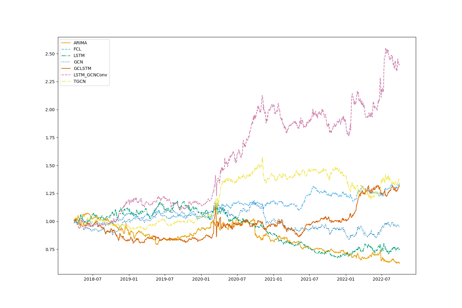
Figure 4: Performance of long-short strategy of all stocks with a restricted country list, stocks return limit at +/- 50%

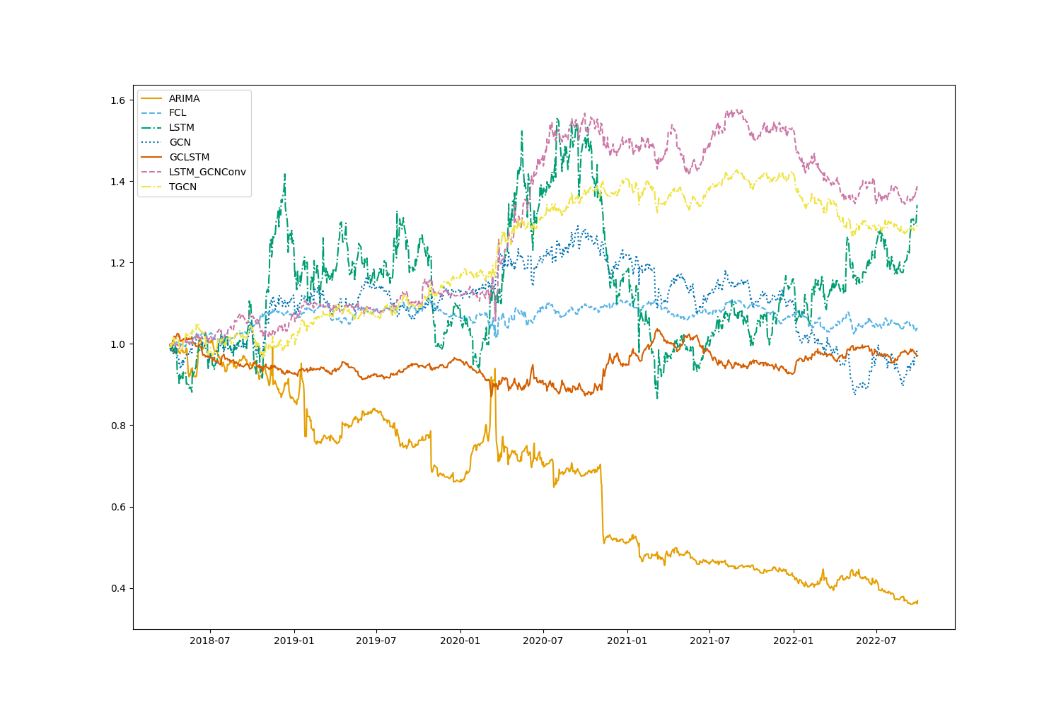
Figure 5: Performance of long-short strategy of all stocks with a restricted country list, stocks return limit at +/- 50%

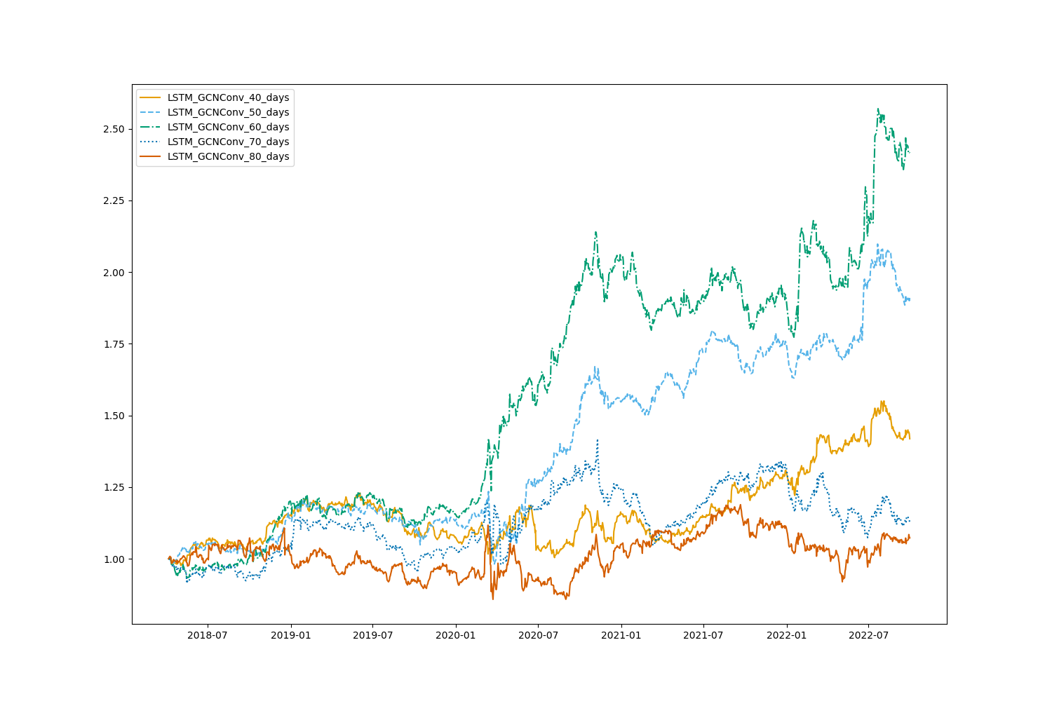
Figure 6: Robustness test on dataset Eurostoxx 600. All simulations show positive annualized returns, Sharpe ratio, and Sortino ratio.

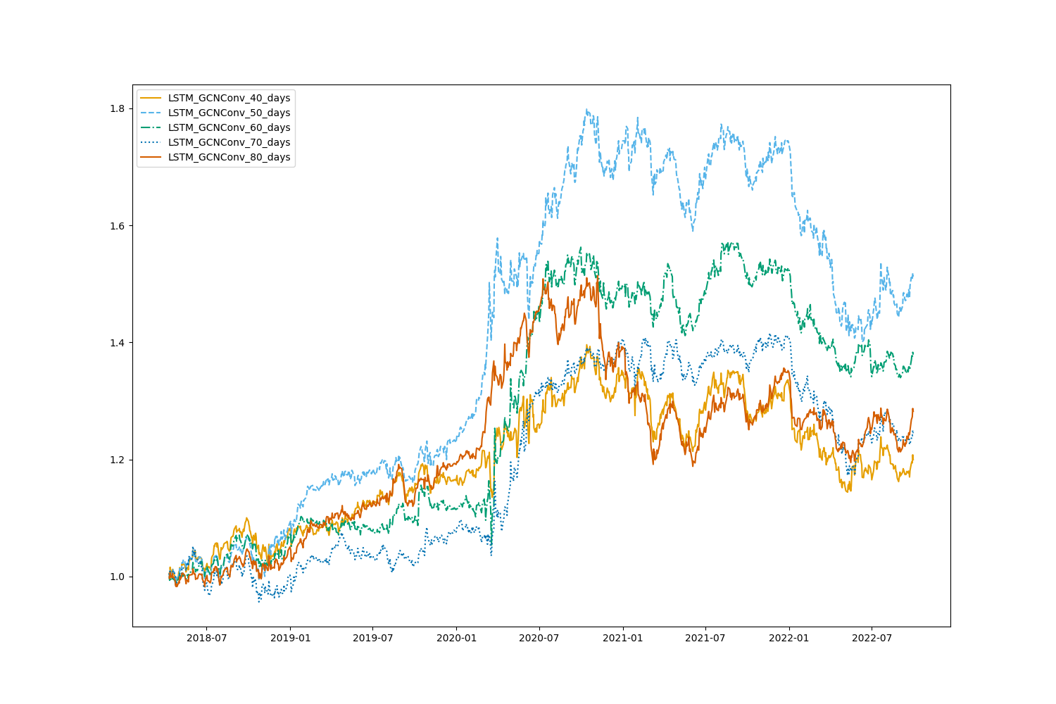
Figure 7: Robustness test on dataset S&P 500. All simulations show positive annualized returns, Sharpe ratio, and Sortino ratio.

TABLE II: Comparison of Models for Eurostoxx 600

models	MAE	MSE	$R^{2}$	Correctness (%)	ann. Return (%)	ann. Sharpe Ratio	ann. Sortino Ratio
ARIMA	8.0733 $10^{-4}$	1.7691 $10^{-2}$	-0.1853	21.2756	-7.8119	-0.5536	-0.6806
FCL	7.2651 $10^{-4}$	1.6716 $10^{-2}$	-0.0123	50.3497	5.0726	0.5787	0.9276
LSTM	7.2118 $10^{-4}$	1.6618 $10^{-2}$	-0.0008	50.3231	-4.8658	-0.3605	-0.5827
GCN	7.2128 $10^{-4}$	1.6639 $10^{-2}$	-0.0017	50.7231	-0.9653	-0.0805	-0.1109
GCLSTM	7.2203 $10^{-4}$	1.6637 $10^{-2}$	-0.0022	50.4616	4.8830	0.2911	0.3366
TGCN	7.2111 $10^{-4}$	1.6614 $10^{-2}$	-0.0007	50.7679	5.5689	0.4153	0.5460
LSTM-GCN	7.1993 $\mathbf{10^{-4}}$	1.6607 $\mathbf{10^{-2}}$	0.0010	51.0170	16.3031	1.0759	1.6872

TABLE III: Comparison of Models for S&P 500

models	MAE	MSE	$R^{2}$	Correctness (%)	ann. Return (%)	ann. Sharpe Ratio	ann. Sortino Ratio
ARIMA	2.0477 $10^{-3}$	2.2001 $10^{-2}$	-0.1569	23.1054	-16.1552	-0.8375	-0.9020
FCL	1.8643 $10^{-3}$	2.1694 $10^{-2}$	-0.0594	50.5791	0.6716	0.0131	0.0164
LSTM	1.8383 $10^{-3}$	2.1024 $10^{-2}$	-0.0005	51.1683	5.3151	0.1890	0.2546
GCN	1.8372 $10^{-3}$	2.1024 $10^{-2}$	-0.0007	51.1574	-0.4178	-0.0859	-0.1224
GCLSTM	1.8745 $10^{-3}$	2.1223 $10^{-2}$	-0.0135	50.5980	-0.5192	-0.1629	-0.2497
TGCN	1.8367 $10^{-3}$	2.1032 $10^{-2}$	-0.0014	50.9658	4.6013	0.5100	0.7920
LSTM-GCN	1.8353 $\mathbf{10^{-3}}$	2.1013 $\mathbf{10^{-2}}$	0.0006	50.9596	5.8904	0.5345	0.8349

TABLE IV: Robustness Test for Eurostoxx 600

length of rolling window	ann. Return (%)	ann. Sharpe Ratio	ann. Sortino Ratio	$R^{2}$	t-statistic	p-value
40	6.2434	0.5200	0.7345	-0.0004	-3.1303	-
50	11.8664	0.9407	1.2455	0.0004	3.4384	3.1476 $10^{-4}$
60	16.4957	1.0956	1.7176	0.0010	7.9738	4.4904 $10^{-15}$
70	2.0968	0.1456	0.1987	0.0005	3.8080	7.7959 $10^{-5}$
80	1.2250	0.0860	0.1099	0.0007	6.0850	1.0933 $10^{-9}$

TABLE V: Robustness Test for S&P 500

length of rolling window	ann. Return (%)	ann. Sharpe Ratio	ann. Sortino Ratio	$R^{2}$	t-statistic	p-value
40	3.2779	0.2592	0.3660	-0.0001	-1.4048	-
50	7.6080	0.6639	0.9638	0.0004	5.0718	2.5690 $10^{-7}$
60	5.8591	0.5307	0.8291	0.0006	6.1369	7.2860 $10^{-10}$
70	3.9570	0.3587	0.5565	-0.0008	-6.5909	-
80	3.4417	0.4180	0.5733	-0.0004	-8.2550	-

V Conclusion

In this paper, we introduce a neural network-based approach LSTM-GCN for stock price prediction, which combines LSTM and GCN. We use a graph network to model the value chain data in which the nodes on the graph represent companies, the edges represent the supplier-customer relationships between companies. The historical performance of the stocks is used as the nodes’ feature/attribute. The GCN is used to capture the topological structure of the graph to obtain the spatial dependencies, while the LSTM model is used to capture the dynamic change of node features to obtain the temporal dependence.

Our experimental results on Eurostoxx 600 and S&P 500 datasets demonstrate the superiority of LSTM-GCN over the baseline models regarding MSE and MAE. We also evaluated the models by running simulations using predicted values for constructing a market-neutral strategy. Results show that our model results in the highest cumulative returns, Sharpe ration, and Sortino ratio. We noticed that the performances of the models differ in the two datasets significantly. We discussed the reason. Overall, we show that for both datasets, even though the amount may vary, excess returns can be found by applying temporal graph models on the value chain data.

Furthermore, we ran a robustness test by varying the length of the rolling window. For each rolling window length, we ran a t-test to evaluate whether $R^{2}$ is significantly larger than zero. Results show that for Eurostoxx 600, rolling window 50, 60, 70, and 80 days, and for S&P 500, rolling window 50, and 60 days, the null hypothesis that $R^{2}\leq 0$ can be rejected, meaning that our model is significantly better than use mean values as predicted values.

Our findings suggest that even though the magnitude of excess returns generated may vary across different datasets, applying temporal graph models on value chain data can be an effective approach to identifying profitable investment opportunities in the stock market. Future research could explore further enhancements to our model, such as incorporating external data sources or applying it to different domains beyond stock price prediction. Especially, we are interested in including additional graphs to the model to have multi-modalities. These could be graphs constructed through data other than from human knowledge, e.g. graphs based on similarity calculated from price data, or heterogeneous graphs with additional entities as nodes other than listed companies e.g. investment managers with a focus on cash equity.

References

- [1] D. P. Gandhmal and K. Kumar, “Systematic analysis and review of stock market prediction techniques,” Computer Science Review, vol. 34, p. 100190, 2019. [Online]. Available: https://www.sciencedirect.com/science/article/pii/S157401371930084X
- [2] R. T. Farias Nazário, J. L. e Silva, V. A. Sobreiro, and H. Kimura, “A literature review of technical analysis on stock markets,” The Quarterly Review of Economics and Finance, vol. 66, pp. 115–126, 2017. [Online]. Available: https://www.sciencedirect.com/science/article/pii/S1062976917300443
- [3] A. A. Ariyo, A. O. Adewumi, and C. K. Ayo, “Stock price prediction using the arima model,” in 2014 UKSim-AMSS 16th International Conference on Computer Modelling and Simulation, 2014, pp. 106–112.
- [4] M. Liu, W.-C. Choo, C.-C. Lee, and C.-C. Lee, “Trading volume and realized volatility forecasting: Evidence from the china stock market,” Journal of Forecasting, vol. 42, no. 1, pp. 76–100, 2023. [Online]. Available: https://onlinelibrary.wiley.com/doi/abs/10.1002/for.2897
- [5] B. Bini and T. Mathew, “Clustering and regression techniques for stock prediction,” Procedia Technology, vol. 24, pp. 1248–1255, 2016, international Conference on Emerging Trends in Engineering, Science and Technology (ICETEST - 2015). [Online]. Available: https://www.sciencedirect.com/science/article/pii/S2212017316301931
- [6] B. G. Malkiel and E. F. Fama, “Efficient capital markets: A review of theory and empirical work*,” The Journal of Finance, vol. 25, no. 2, pp. 383–417, 1970. [Online]. Available: https://onlinelibrary.wiley.com/doi/abs/10.1111/j.1540-6261.1970.tb00518.x
- [7] M. de Prado, Machine Learning for Asset Managers, ser. Elements in Quantitative Finance. Cambridge University Press, 2020. [Online]. Available: https://books.google.de/books?id=0D8LEAAAQBAJ
- [8] Y. Lecun, L. Bottou, Y. Bengio, and P. Haffner, “Gradient-based learning applied to document recognition,” Proceedings of the IEEE, vol. 86, no. 11, pp. 2278–2324, 1998.
- [9] A. Krizhevsky, I. Sutskever, and G. E. Hinton, “Imagenet classification with deep convolutional neural networks,” Commun. ACM, vol. 60, no. 6, p. 84–90, may 2017. [Online]. Available: https://doi.org/10.1145/3065386
- [10] T. N. Kipf and M. Welling, “Semi-supervised classification with graph convolutional networks,” arXiv preprint arXiv:1609.02907, 2016.
- [11] F. D. Paiva, R. T. N. Cardoso, G. P. Hanaoka, and W. M. Duarte, “Decision-making for financial trading: A fusion approach of machine learning and portfolio selection,” Expert Systems with Applications, vol. 115, pp. 635–655, 2019. [Online]. Available: https://www.sciencedirect.com/science/article/pii/S0957417418305037
- [12] J. Eapen, D. Bein, and A. Verma, “Novel deep learning model with cnn and bi-directional lstm for improved stock market index prediction,” in 2019 IEEE 9th Annual Computing and Communication Workshop and Conference (CCWC), 2019, pp. 0264–0270.
- [13] M. A. Hossain, R. Karim, R. Thulasiram, N. D. B. Bruce, and Y. Wang, “Hybrid deep learning model for stock price prediction,” in 2018 IEEE Symposium Series on Computational Intelligence (SSCI), 2018, pp. 1837–1844.
- [14] K. Chen, Y. Zhou, and F. Dai, “A lstm-based method for stock returns prediction: A case study of china stock market,” in 2015 IEEE International Conference on Big Data (Big Data), 2015, pp. 2823–2824.
- [15] B. Lei, Z. Liu, and Y. Song, “On stock volatility forecasting based on text mining and deep learning under high-frequency data,” Journal of Forecasting, vol. 40, no. 8, pp. 1596–1610, 2021. [Online]. Available: https://onlinelibrary.wiley.com/doi/abs/10.1002/for.2794
- [16] S. Borovkova and I. Tsiamas, “An ensemble of lstm neural networks for high-frequency stock market classification,” Journal of Forecasting, vol. 38, no. 6, pp. 600–619, 2019. [Online]. Available: https://onlinelibrary.wiley.com/doi/abs/10.1002/for.2585
- [17] J. M.-T. Wu, Z. Li, G. Srivastava, M.-H. Tasi, and J. C.-W. Lin, “A graph-based convolutional neural network stock price prediction with leading indicators,” Software: Practice and Experience, vol. 51, no. 3, pp. 628–644, 2021. [Online]. Available: https://onlinelibrary.wiley.com/doi/abs/10.1002/spe.2915
- [18] J.-E. Choi and D. W. Shin, “Parallel architecture of cnn-bidirectional lstms for implied volatility forecast,” Journal of Forecasting, vol. 41, no. 6, pp. 1087–1098, 2022. [Online]. Available: https://onlinelibrary.wiley.com/doi/abs/10.1002/for.2844
- [19] M. Defferrard, X. Bresson, and P. Vandergheynst, “Convolutional neural networks on graphs with fast localized spectral filtering,” CoRR, vol. abs/1606.09375, 2016. [Online]. Available: http://arxiv.org/abs/1606.09375
- [20] Y. Seo, M. Defferrard, P. Vandergheynst, and X. Bresson, “Structured sequence modeling with graph convolutional recurrent networks,” 12 2016. [Online]. Available: http://arxiv.org/abs/1612.07659
- [21] L. Ruiz, F. Gama, and A. Ribeiro, “Gated graph recurrent neural networks,” IEEE Transactions on Signal Processing, vol. 68, pp. 6303–6318, 2020. [Online]. Available: https://doi.org/10.1109%2Ftsp.2020.3033962
- [22] T. N. Kipf and M. Welling, “Semi-supervised classification with graph convolutional networks,” 2016. [Online]. Available: https://arxiv.org/abs/1609.02907
- [23] Q. Chen and C.-Y. Robert, “Graph-based learning for stock movement prediction with textual and relational data,” The Journal of Financial Data Science, vol. 4, no. 4, pp. 152–166, 2022. [Online]. Available: https://jfds.pm-research.com/content/4/4/152
- [24] B. Son, Y. Lee, S. Park, and J. Lee, “Forecasting global stock market volatility: The impact of volatility spillover index in spatial-temporal graph-based model,” Journal of Forecasting, vol. n/a, no. n/a. [Online]. Available: https://onlinelibrary.wiley.com/doi/abs/10.1002/for.2975
- [25] L. Cohen, A. Frazzini, J. Chevalier, K. Daniel, D. Diamond, G. Fama, W. Goetzmann, R. Jagannathan, A. Kashyap, J. Lakonishok, O. Lamont, J. Lewellen, T. Moskowitz, L. Pedersen, M. Piazzesi, J. Piotroski, J. Rauh, D. Skinner, M. Spiegel, R. Stambaugh, A. Sufi, J. Thomas, T. Vuolteenaho, I. Welch, and W. Xiong, “Economic links and predictable returns,” 2008.
- [26] Y. Wang, Y. Qu, and Z. Chen, “Review of graph construction and graph learning in stock price prediction,” Procedia Computer Science, vol. 214, pp. 771–778, 2022, 9th International Conference on Information Technology and Quantitative Management. [Online]. Available: https://www.sciencedirect.com/science/article/pii/S1877050922019500
- [27] J. Gao, X. Ying, C. Xu, J. Wang, S. Zhang, and Z. Li, “Graph-based stock recommendation by time-aware relational attention network,” ACM Trans. Knowl. Discov. Data, vol. 16, no. 1, jul 2021. [Online]. Available: https://doi.org/10.1145/3451397
- [28] C. Xu, H. Huang, X. Ying, J. Gao, Z. Li, P. Zhang, J. Xiao, J. Zhang, and J. Luo, “Hgnn: Hierarchical graph neural network for predicting the classification of price-limit-hitting stocks,” Information Sciences, vol. 607, pp. 783–798, 2022. [Online]. Available: https://www.sciencedirect.com/science/article/pii/S0020025522005928
- [29] W. Li, R. Bao, K. Harimoto, D. Chen, J. Xu, and Q. Su, “Modeling the stock relation with graph network for overnight stock movement prediction,” in Proceedings of the Twenty-Ninth International Joint Conference on Artificial Intelligence, IJCAI-20, C. Bessiere, Ed. International Joint Conferences on Artificial Intelligence Organization, 7 2020, pp. 4541–4547, special Track on AI in FinTech. [Online]. Available: https://doi.org/10.24963/ijcai.2020/626
- [30] R. Cheng and Q. Li, “Modeling the momentum spillover effect for stock prediction via attribute-driven graph attention networks,” Proceedings of the AAAI Conference on Artificial Intelligence, vol. 35, no. 1, pp. 55–62, May 2021. [Online]. Available: https://ojs.aaai.org/index.php/AAAI/article/view/16077
- [31] L. Lai, C. Li, and W. Long, “A new method for stock price prediction based on mrfs and ssvm,” in 2017 IEEE International Conference on Data Mining Workshops (ICDMW), 2017, pp. 818–823.
- [32] C. K.-S. Leung, R. K. MacKinnon, and Y. Wang, “A machine learning approach for stock price prediction,” in Proceedings of the 18th International Database Engineering & Applications Symposium, ser. IDEAS ’14. New York, NY, USA: Association for Computing Machinery, 2014, p. 274–277. [Online]. Available: https://doi.org/10.1145/2628194.2628211
- [33] M. Defferrard, X. Bresson, and P. Vandergheynst, “Convolutional neural networks on graphs with fast localized spectral filtering,” 2016. [Online]. Available: https://arxiv.org/abs/1606.09375
- [34] T. G. Smith et al., “pmdarima: Arima estimators for Python,” 2017–, [Online; accessed ¡today¿]. [Online]. Available: http://www.alkaline-ml.com/pmdarima
- [35] J. Chen, X. Wang, and X. Xu, “Gc-lstm: Graph convolution embedded lstm for dynamic link prediction,” 12 2018. [Online]. Available: http://arxiv.org/abs/1812.04206
- [36] L. Zhao, Y. Song, C. Zhang, Y. Liu, P. Wang, T. Lin, M. Deng, and H. Li, “T-GCN: A temporal graph convolutional network for traffic prediction,” IEEE Transactions on Intelligent Transportation Systems, vol. 21, no. 9, pp. 3848–3858, sep 2020. [Online]. Available: https://doi.org/10.1109%2Ftits.2019.2935152
- [37] S. Gu, B. Kelly, and D. Xiu, “Empirical Asset Pricing via Machine Learning,” The Review of Financial Studies, vol. 33, no. 5, pp. 2223–2273, 02 2020. [Online]. Available: https://doi.org/10.1093/rfs/hhaa009
- [38] W. F. Sharpe, “The sharpe ratio,” The Journal of Portfolio Management, vol. 21, no. 1, pp. 49–58, 1994. [Online]. Available: https://jpm.pm-research.com/content/21/1/49
- [39] F. A. Sortino and R. van der Meer, “Downside risk,” The Journal of Portfolio Management, vol. 17, no. 4, pp. 27–31, 1991. [Online]. Available: https://jpm.pm-research.com/content/17/4/27