A parsimonious neural network approach to solve portfolio optimization problems without using dynamic programming

Abstract

We present a parsimonious neural network approach, which does not rely on dynamic programming techniques, to solve dynamic portfolio optimization problems subject to multiple investment constraints. The number of parameters of the (potentially deep) neural network remains independent of the number of portfolio rebalancing events, and in contrast to, for example, reinforcement learning, the approach avoids the computation of high-dimensional conditional expectations. As a result, the approach remains practical even when considering large numbers of underlying assets, long investment time horizons or very frequent rebalancing events. We prove convergence of the numerical solution to the theoretical optimal solution of a large class of problems under fairly general conditions, and present ground truth analyses for a number of popular formulations, including mean-variance and mean-conditional value-at-risk problems. We also show that it is feasible to solve Sortino ratio-inspired objectives (penalizing only the variance of wealth outcomes below the mean) in dynamic trading settings with the proposed approach. Using numerical experiments, we demonstrate that if the investment objective functional is separable in the sense of dynamic programming, the correct time-consistent optimal investment strategy is recovered, otherwise we obtain the correct pre-commitment (time-inconsistent) investment strategy. The proposed approach remains agnostic as to the underlying data generating assumptions, and results are illustrated using (i) parametric models for underlying asset returns, (ii) stationary block bootstrap resampling of empirical returns, and (iii) generative adversarial network (GAN)-generated synthetic asset returns.

Keywords: Asset allocation, portfolio optimization, neural network, dynamic programming

JEL classification: G11, C61

1 Introduction

We present, and analyze the convergence of, a parsimonious and flexible neural network approach to obtain the numerical solution of a large class of dynamic (i.e. multi-period) portfolio optimization problems that can be expressed in the following form,

$$\inf_{\xi\in\mathbb{R}}\inf_{\mathcal{P}\in\mathcal{A}}\left\{\>E_{\mathcal{P}}^{t_{0},w_{0}}\left[F\left(W\left(T\right),\xi\right)+G\left(W\left(T\right),E_{\mathcal{P}}^{t_{0},w_{0}}\left[W\left(T\right)\right],w_{0},\xi\right)\begin{array}[]{c}\!\!\!\!\!\!\!\!\\ \!\!\!\!\!\!\!\!\end{array}\right]\>\right\}.$$ (1.1)

While rigorous definitions and assumptions are discussed in subsequent sections, here we simply note that in general, $F:\mathbb{R}^{2}\rightarrow\mathbb{R}$ and $G:\mathbb{R}^{4}\rightarrow\mathbb{R}$ denote some continuous functions and $\xi\in\mathbb{R}$ some auxiliary variable, with $T>0$ denoting the investment time horizon, $W\left(t\right),t\in\left[t_{0},T\right]$, the controlled wealth process, and $\mathcal{P}$ representing the investment strategy (or control) implemented over $\left[t_{0},T\right]$. Typically, $\mathcal{P}$ specifies the amount or fraction of wealth to invest in each of (a potentially large number of) the underlying assets at each portfolio rebalancing event, which in practice occurs at some discrete subset of rebalancing times in $\left[t_{0},T\right]$. $\mathcal{A}$ denotes the set of admissible investment strategies encoding the (possibly multiple) investment constraints faced by the investor. Finally, $E_{\mathcal{P}}^{t_{0},w_{0}}\left[\cdot\right]$ denotes the expectation given control $\mathcal{P}$ and initial wealth $W\left(t_{0}\right)=w_{0}$.

Although (1.1) is written for objective functions involving the terminal portfolio wealth $W\left(T\right)$, the approach and convergence analysis could be generalized without difficulty to objective functions that are wealth path-dependent, i.e. functions of $\left\{W\left(t\right):t\in\mathcal{T}\right\}$ for some subset $\mathcal{T}\subseteq\left[t_{0,}T\right]$ - see Forsyth et al. (2022); Van Staden et al. (2022a) for examples. However, since a sufficiently rich class of problems are of the form (1.1), this will remain the main focus of this paper.

The proposed approach does not rely on the separability of the objective functional in (1.1) in the sense of dynamic programming, remains agnostic as to the underlying data generation assumptions, and is sufficiently flexible such that practical considerations such as multiple investment constraints and discrete portfolio rebalancing can be incorporated without difficulty.

Leaving the more formal treatment for subsequent sections, for introductory purposes we highlight some specific examples of problems of the form (1.1):

1. Utility maximization (see for example Vigna (2014)), in which case there is no outer optimization problem and $G\equiv 0$, while $w\rightarrow U\left(w\right)$ denotes the investor’s utility function, so that (1.1) therefore reduces to

   $$\sup_{\mathcal{P}\in\mathcal{A}}\left\{E_{\mathcal{P}}^{t_{0},w_{0}}\left[U\left(W\left(T\right)\right)\right]\right\}.$$ (1.2)

2. Mean-variance (MV) optimization (see e.g. Zhou and Li (2000); Li and Ng (2000)), with $\rho>0$ denoting the scalarization (or risk aversion) parameter, where the problem

   $$\sup_{\mathcal{P}\in\mathcal{A}}\left\{E_{\mathcal{P}}^{t_{0},w_{0}}\left[W\left(T\right)\right]-\rho\cdot Var_{\mathcal{P}}^{t_{0},w_{0}}\left[W\left(T\right)\right]\right\},$$ (1.3)

   can also be written in the general form (1.1).

3. Mean-Conditional Value-at-Risk (CVaR) optimization, in which case we do have both an inner and an outer optimization problems (see e.g. Miller and Yang (2017); Forsyth (2020), resulting in a problem of the form

   $$\inf_{\xi\in\mathbb{R}}\inf_{\mathcal{P}\in\mathcal{A}}\left\{E_{\mathcal{P}}^{t_{0},w_{0}}\left[F\left(W\left(T\right),\xi\right)\right]\right\},$$ (1.4)

   for a particular choice of the function $F$ (see (2.17) below).

4. To illustrate the flexibility and generality of the proposed approach, we also consider a “mean semi-variance” portfolio optimization problem that is inspired by the popular Sortino ratio (Bodie et al. (2014)) in the case of one-period portfolio analysis, where only the variance of downside outcomes relative to the mean is penalized. In the case of dynamic trading strategies, this suggests an objective function of the form

   $$\sup_{\mathcal{P}\in\mathcal{A}}\left\{E_{\mathcal{P}}^{t_{0},w_{0}}\left[W\left(T\right)-\rho\cdot\left(\min\left\{W\left(T\right)-E_{\mathcal{P}}^{t_{0},w_{0}}\left[W\left(T\right)\right],0\right\}\right)^{2}\right]\right\},$$ (1.5)

   where, as in the case of (1.3), the parameter $\rho>0$ encodes the trade-off between risk and return. Note that (1.5) is not separable in the sense of dynamic programming, and in the absence of embedding results (analogous to those of Zhou and Li (2000); Li and Ng (2000) in the case of MV optimization (1.3)), problem (1.5) cannot be solved using traditional dynamic programming-based methods.

However, we emphasize that (1.2)-(1.5) are only a selection of examples, and the proposed approach and theoretical analysis remains applicable to problems that can be expressed in the general form (1.1).

Portfolio optimization problems of the form (1.1) can give rise to investment strategies that are not time-consistent due to the presence of the (possibly non-linear) function $G$ (Bjork et al. (2021)). Since the objective in (1.1) is therefore potentially not separable in the sense of dynamic programming (see for example (1.3) or (1.5)). This gives rise to two related problems: (i) Since (1.1) cannot be solved using a dynamic programming-based approach, some other solution methodology has to be implemented, or some re-interpretation of the problem or the concept of “optimality” might be required (see for example Vigna (2022); Bjork and Murgoci (2014)), (ii) if the investment strategies are time-inconsistent, this can raise questions as to whether these strategies are feasible to implement as practical investment strategies.

We make the following general observations:

• It may be desirable to avoid using dynamic programming (DP) even if (1.1) can be solved using DP techniques, such as in the special case where $G\equiv 0$ in (1.1) and the investment strategies are time-consistent. For example, it is well known that DP has an associated “curse of dimensionality”, in that as the number state variables increases linearly, the computational burden increases exponentially (Han and Weinan (2016); Fernández-Villaverde et al. (2020)). In addition, since DP techniques necessarily incur estimation errors at each time step, significant error amplification can occur which is further exacerbated in high-dimensional settings (see for example Wang and Foster (2020); Tsang and Wong (2020); Li et al. (2020)).

  However, instead of relying on DP-based techniques and attempting to address the challenges of dimensionality using machine learning techniques (see for example Dixon et al. (2020); Park et al. (2020); Lucarelli and Borrotti (2020); Gao et al. (2020); Fernández-Villaverde et al. (2020); Henry-Labordère (2017); Huré et al. (2021); Bachouch et al. (2022)), the proposed method fundamentally avoids DP techniques altogether. This is especially relevant in our setting, since we have shown that in the case of portfolio optimization problems specifically, DP can be unnecessarily high-dimensional even in simple settings (see Van Staden et al. (2022b)). This occurs since the objective functional (or performance criteria (Oksendal and Sulem (2019)) ) is typically high-dimensional while the optimal investment strategy (the fundamental quantity of concern) remains relatively low-dimensional. The proposed method therefore forms part of the significant recent interest in developing machine learning techniques to solve multi-period portfolio optimization problems that avoids using DP techniques altogether (see for example Li and Forsyth (2019); Tsang and Wong (2020); Van Staden et al. (2022b); Ni et al. (2022)).

• Time-inconsistent problems naturally arise in financial applications (see Bjork et al. (2021) for numerous examples), and as a result their solution is often an area of active research due to the unique challenges involved in solving these problems without resorting to DP techniques. Examples include the mean-variance problem, which remained an open problem for decades until the solution using the embedding technique of Zhou and Li (2000); Li and Ng (2000). As a result, being able to obtain a numerical solution to problems of the form (1.1) directly is potentially very valuable for research.

  The solution of time-inconsistent problems is also practical interest, since in many cases, there exists an induced time consistent objective function (Strub et al. (2019b, a); Forsyth (2020)). The optimal policy for this induced time consistent objective function is identical to the pre-commitment policy at time zero. The induced time consistent strategy is, of course implementable (Forsyth (2020)), in the sense that the investor has no incentive to deviate from the strategy determined at time zero, at later times.

  An alternative approach to handling time-inconsistent problems is to search for the equilibrium control (Bjork et al. (2021)). A fascinating result obtained in Bjork and Murgoci (2010) is that for every equilibrium control, there exists a standard, time consistent problem which has the same control, under a different objective function.

  This essentially means that the question of time-consistency is a often matter of perspective, since there may be alternative objective functions which give rise to the same pre-commitment control, yet are time-consistent. In fact, other subtle issues arise in comparing pre-commitment and time consistent controls, see Vigna (2020, 2022) for further discussion.

  Furthermore, over very short time horizons such as those encountered in optimal trade execution, time consistency or its absence may not be of much concern to the investor or market participant (see for example Forsyth et al. (2011); Tse et al. (2013)).

  In addition, as noted by Bernard and Vanduffel (2014), if the strategy is realized in an investment product sold to a retail investor, then the optimal policy from the investor’s point of view is in fact of pre-commitment type, since the retail client does not herself trade in the underlying assets during the lifetime of the contract.

As a result of these observations, we will consider problem (1.1) in its general form. Our method builds on and formalizes the initial results described in Li and Forsyth (2019) where a shallow NN was applied to a portfolio optimization problem with an objective that is separable in the sense of DP. The contributions of this paper are as follows:

1. We present a flexible neural network (NN) approach to solve problems of the form (1.1) that does not rely on DP techniques. Our approach only requires the solution of a single optimization problem, and therefore avoids the error amplification problems associated with the time-recursion in DP-based techniques, including for example Reinforcement Learning algorithms such as Q-learning (see for example Park et al. (2020); Dixon et al. (2020); Gao et al. (2020)) or other algorithms relying at some level on the DP principle for a time-stepping backward recursion (see for example Bachouch et al. (2022); Van Heeswijk and Poutré (2019)). Perhaps the best descriptor of our approach is Policy Function Approximation, in the taxonomy in Powell (2023).

   We make very limited assumptions regarding the underlying asset dynamics. In particular, if underlying asset (and by extension wealth) dynamics are specified, this can be incorporated as easily as the case where the underlying dynamics can only be observed without any parametric assumptions.

   The proposed solution methodology is parsimonious, in that the number of parameters does not scale with the number of rebalancing events. This contrasts the proposed methodology with for example that of Han and Weinan (2016); Tsang and Wong (2020); Huré et al. (2021), and ensures that our approach remains feasible even for problems with very long time horizons (for example the accumulation phase of a pension fund - see Forsyth et al. (2019)) or with shorter time horizon but with frequent trading/rebalancing (for example the trade execution problems encountered in Forsyth et al. (2011)). The solution approach only places very weak requirements on the form of the investment objective in (1.1). In addition, we find that using relatively shallow neural networks (at most two hidden layers) in our approach achieve very accurate results in ground truth testing, thereby ensuring that the resulting NN in the proposed approach is relatively easy and efficient to train since it is less likely to be susceptible to problems of vanishing or exploding gradients associated with very deep neural networks (Goodfellow et al. (2016)).

2. We analyze the convergence of the proposed approach, and show that the theoretical optimal investment strategy of (1.1), provided it exists, can be attained by the numerical solution.

3. Finally, we present ground truth analyses confirming that the proposed approach is very effective in solving portfolio optimization problems of the form (1.1). The results illustrate numerically that if (1.1) is not separable in the sense of DP, our approach recovers the correct pre-commitment (time-inconsistent) optimal control, otherwise it recovers the correct time-consistent optimal control. To emphasize that the approach remains agnostic to the underlying data generation assumptions, results are illustrated using (i) parametric models for asset dynamics, (ii) stationary block bootstrap resampling of empirical asset returns, and (ii) generative adversarial network (GAN)-generated synthetic asset returns.

The remainder of the paper is organized as follows: Section 2 presents the problem formulation, while Section 3 provides a summary of the proposed approach, with additional technical and practical details provided in Appendix A and Appendix B. Section 4 presents the convergence analysis of the proposed approach. Finally, Section 5 provides ground truth analyses, with Section 6 concluding the paper and discussing possible avenues for future research.

2 Problem formulation

We start by formulating portfolio optimization problems of the form (1.1) more rigorously in a setting of discrete portfolio rebalancing and multiple investment constraints. Throughout, we work on filtered probability space $\left(\Omega,\mathcal{F},\left\{\mathcal{F}\left(t\right)\right\}_{t\in\left[t_{0},T\right]},\mathbb{P}\right)$ satisfying the usual conditions, with $\mathbb{P}$ denoting the actual (and not the risk-neutral) probability measure.

Let $\mathcal{T}$ denote the set of $N_{rb}$ discrete portfolio rebalancing times in $\left[t_{0}=0,T\right]$, which we assume to be equally-spaced to lighten notation,

$$\mathcal{\mathcal{T}} = \left\{\left.t_{m}=m\Delta t\right|m=0,...,N_{rb}-1\right\},\qquad\Delta t=T/N_{rb},$$ (2.1)

where we observe that the last rebalancing event occurs at time $t_{N_{rb}-1}=T-\Delta t$.

At each rebalancing time $t_{m}\in\mathcal{T}$, the investor observes the $\mathcal{F}\left(t_{m}\right)$-measurable vector $\boldsymbol{X}\left(t_{m}\right)=\left(X_{i}\left(t_{m}\right):i=1,...,\eta_{X}\right)\in\mathbb{R}^{\eta_{X}}$, which can be interpreted informally as the information taken into account by the investor in reaching their asset allocation decision. As a concrete example, we assume below that $\boldsymbol{X}\left(t_{m}\right)$ includes at least the wealth available for investment, an assumption which can be rigorously justified using analytical results (see for example Van Staden et al. (2022b)).

Given $\boldsymbol{X}\left(t_{m}\right)$, the investor then rebalances a portfolio of $N_{a}$ assets to new positions given by the vector

$$\boldsymbol{p}_{m}\left(t_{m},\boldsymbol{X}\left(t_{m}\right)\right) = \left(p_{m,i}\left(t_{m},\boldsymbol{X}\left(t_{m}\right)\right):i=1,..,N_{a}\right)\in\mathbb{R}^{N_{a}},$$ (2.2)

where $p_{m,i}\left(t_{m},\boldsymbol{X}\left(t_{m}\right)\right)$ denotes the fraction of wealth $W\left(t_{m}\right)$ invested in the $i$th asset at rebalancing time $t_{m}$. The subscript “$m$” in the notation $\boldsymbol{p}_{m}$ emphasizes that in general, each rebalancing time $t_{m}\in\mathcal{T}$ could be associated with potentially a different function $\boldsymbol{p}_{m}:\mathbb{R}^{\eta_{X}+1}\rightarrow\mathbb{R}^{N_{a}}$, while the subscript is removed below when we consider a single function that is simply evaluated at different times, in which case we will write $\boldsymbol{p}:\mathbb{R}^{\eta_{X}+1}\rightarrow\mathbb{R}^{N_{a}}$.

For purposes of concreteness, we assume that the investor is subject to the constraints of (i) no short-selling and (ii) no leverage being allowed, although the proposed methodology can be adjusted without difficulty to treat different constraint formulations. For illustrative purposes, we therefore assume that each allocation (2.2) is only allowed to take values in $\left(N_{a}-1\right)$-dimensional probability simplex $\mathcal{Z}$,

$$\mathcal{Z} = \left\{\left(y_{1},...,y_{N_{a}}\right)\in\mathbb{R}^{N_{a}}:\sum_{i=1}^{N_{a}}y_{i}=1\textrm{ and }y_{i}\geq 0\textrm{ for all }i=1,...,N_{a}\right\}.$$ (2.3)

In this setting, an investment strategy or control $\mathcal{P}$ applicable to $\left[t_{0},T\right]$ is therefore of the form,

$$\mathcal{P} = \left\{\boldsymbol{p}_{m}\left(t_{m},\boldsymbol{X}\left(t_{m}\right)\right)=\left(p_{m,i}\left(t_{m},\boldsymbol{X}\left(t_{m}\right)\right):i=1,..,N_{a}\right):t_{m}\in\mathcal{T}\right\},$$ (2.4)

while the set of admissible controls $\mathcal{A}$ is defined by

$$\mathcal{A} = \left\{\left.\mathcal{P}=\left\{\boldsymbol{p}_{m}\left(t_{m},\boldsymbol{X}\left(t_{m}\right)\right):t_{m}\in\mathcal{T}\right\}\right|\boldsymbol{p}_{m}\left(t_{m},\boldsymbol{X}\left(t_{m}\right)\right)\in\mathcal{Z},\forall t_{m}\in\mathcal{T}\right\}.$$ (2.5)

The randomness in the system is introduced through the returns of the underlying assets. Specifically, let $R_{i}\left(t_{m}\right)$ denote the $\mathcal{F}\left(t_{m+1}\right)$-measurable return observed on asset $i$ over the interval $\left[t_{m},t_{m+1}\right]$. We make no assumptions regarding the underlying asset dynamics, but at a minimum, we do require ($\mathbb{P}$) integrability, i.e. $\mathbb{E}\left|R_{i}\left(t_{m}\right)\right|<\infty$ for all $i\in\left\{1,...,N_{a}\right\}$ and $m\in\left\{0,...,N_{rb}-1\right\}$. Informally, we will refer to the set

$$\boldsymbol{Y} = \left\{\left(Y_{i}\left(t_{m}\right)\coloneqq 1+R_{i}\left(t_{m}\right):i=1,...,N_{a}\right)^{\top}:m\in\left\{0,...,N_{rb}-1\right\}\right\}$$ (2.6)

as the path of (joint) asset returns over the investment time horizon $\left[t_{0},T\right]$.

To clarify the subsequent notation, for any functional $\psi\left(t\right),t\in\left[t_{0},T\right]$ we will use the notation $\psi\left(t^{-}\right)$ and $\psi\left(t^{+}\right)$ as shorthand for the one-sided limits $\psi\left(t^{-}\right)=\lim_{\epsilon\downarrow 0}\psi\left(t-\epsilon\right)$ and $\psi\left(t^{+}\right)=\lim_{\epsilon\downarrow 0}\psi\left(t+\epsilon\right)$, respectively.

Given control $\mathcal{P}\in\mathcal{A}$, asset returns $\boldsymbol{Y}$, initial wealth $W\left(t_{0}^{-}\right)\coloneqq w_{0}>0$ and a (non-random) cash contribution schedule $\left\{q\left(t_{m}\right):t_{m}\in\mathcal{T}\right\}$, the portfolio wealth dynamics for $m=0,...,N_{rb}-1$ are given by the general recursion

$$W\left(t_{m+1}^{-};\mathcal{P},\boldsymbol{Y}\right) = \left[W\left(t_{m}^{-};\mathcal{P},\boldsymbol{Y}\right)+q\left(t_{m}\right)\right]\cdot\sum_{i=1}^{N_{a}}p_{m,i}\left(t_{m},\boldsymbol{X}\left(t_{m}\right)\right)\cdot Y_{i}\left(t_{m}\right).$$ (2.7)

Note that we write $W\left(u\right)=W\left(u;\mathcal{P},\boldsymbol{Y}\right)$ to emphasize the dependence of wealth on the control $\mathcal{P}$ and the (random) path of asset returns in $\boldsymbol{Y}$ that relates to the time period $t\in\left[t_{0},u\right]$. In other words, despite using $\boldsymbol{Y}$ in the notation for simplicity, $W\left(u;\mathcal{P},\boldsymbol{Y}\right)$ is $\mathcal{F}\left(u\right)$-measurable. Finally, since there are no contributions or rebalancing at maturity, we simply have $W\left(t_{N_{rb}}^{-}\right)=W\left(T^{-}\right)=W\left(T\right)=W\left(T;\mathcal{P},\boldsymbol{Y}\right)$.

2.1 Investment objectives

Given this general investment setting and wealth dynamics (2.7), our goal is to solve dynamic portfolio optimization problems of the general form

$$\inf_{\xi\in\mathbb{R}}\inf_{\mathcal{P}\in\mathcal{A}}J\left(\mathcal{P},\xi;t_{0},w_{0}\right),$$ (2.8)

where, for some given continuous functions $F:\mathbb{R}^{2}\rightarrow\mathbb{R}$ and $G:\mathbb{R}^{3}\rightarrow\mathbb{R}$, the objective functional $J$ is given by

$$J\left(\mathcal{P},\xi;t_{0},w_{0}\right) = E_{\mathcal{P}}^{t_{0},w_{0}}\left[F\left(W\left(T;\mathcal{P},\boldsymbol{Y}\right),\xi\right)+G\left(W\left(T;\mathcal{P},\boldsymbol{Y}\right),E_{\mathcal{P}}^{t_{0},w_{0}}\left[W\left(T;\mathcal{P},\boldsymbol{Y}\right)\right],w_{0},\xi\right)\begin{array}[]{c}\!\!\!\!\!\!\!\!\\ \!\!\!\!\!\!\!\!\end{array}\right].$$ (2.11)

Note that the expectations $E^{t_{0},w_{0}}\left[\cdot\right]$ in (2.11) are taken over $\boldsymbol{Y}$, given initial wealth $W\left(t_{0}^{-}\right)=w_{0}$, control $\mathcal{P}\in\mathcal{A}$ and auxiliary variable $\xi\in\mathbb{R}$. In addition to the assumption of continuity of $F$ and $G$, we will make only the minimal assumptions regarding the exact properties of $J$, including that $\xi\rightarrow F\left(\cdot,\xi\right)$ and $\xi\rightarrow G\left(\cdot,\cdot,w_{0},\xi\right)$ are convex for all admissible controls $\mathcal{P}\in\mathcal{A}$, and the standard assumption (see for example Bjork et al. (2021)) that an optimal control $\mathcal{P}^{\ast}\in\mathcal{A}$ exists.

For illustrative and ground truth analysis purposes, we consider a number of examples of problems of the form (2.8)-(2.11).

As noted in the Introduction, the simplest examples of problems of the form (2.8) arise in the special case where $G\equiv 0$ and there is no outer optimization problem over $\xi$, such as in the case of standard utility maximization problems. As concrete examples of this class of objective functions, we will consider the quadratic target minimization (or quadratic utility) described in for example Vigna (2014); Zhou and Li (2000),

$$\left(DSQ\left(\gamma\right)\right): \inf_{\mathcal{P}\in\mathcal{A}}\left\{E^{t_{0},w_{0}}\left[\left(W\left(T;\mathcal{P},\boldsymbol{Y}\right)-\gamma\right)^{2}\right]\right\},\qquad\gamma>0,$$ (2.12)

as well as the (closely-related) one-sided quadratic loss minimization used in for example Dang and Forsyth (2016); Li and Forsyth (2019),

$$\left(OSQ\left(\gamma\right)\right):\qquad \inf_{\mathcal{P}\in\mathcal{A}}\left\{E^{t_{0},w_{0}}\left[\left(\min\left\{W\left(T;\mathcal{P},\boldsymbol{Y}\right)-\gamma,0\right\}\right)^{2}-\epsilon\cdot W\left(T;\mathcal{P},\boldsymbol{Y}\right)\right]\right\},\qquad\gamma>0.$$ (2.13)

The term $\epsilon W(\cdot)$ in equation (2.13) ensures that the problem remains well-posed in the event that $W(t)\gg\gamma$. Observe that problems of the form (2.12) or (2.13) are separable in the sense of dynamic programming, so that the resulting optimal control is therefore time-consistent.

As a classical example of the case where $G$ is nonlinear and the objective functional (2.11) is not separable in the sense of dynamic programming, we consider the mean-variance (MV) objective with scalarization or risk-aversion parameter $\rho>0$ (see for example Bjork et al. (2017)),

$$\left(MV\left(\rho\right)\right): \sup_{\mathcal{P}\in\mathcal{A}}\left\{E^{t_{0},w_{0}}\left[W\left(T;\mathcal{P},\boldsymbol{Y}\right)\right]-\rho\cdot Var^{t_{0},w_{0}}\left[W\left(T;\mathcal{P},\boldsymbol{Y}\right)\right]\right\},\qquad\rho>0.$$ (2.14)

$$= \sup_{\mathcal{P}\in\mathcal{A}}E_{\mathcal{P}}^{t_{0},w_{0}}\left[W\left(T;\mathcal{P},\boldsymbol{Y}\right)-\rho\cdot\left(W\left(T;\mathcal{P},\boldsymbol{Y}\right)-E_{\mathcal{P}}^{t_{0},w_{0}}\left[W\left(T;\mathcal{P},\boldsymbol{Y}\right)\right]\right)^{2}\right].$$

Note that issues relating to the time-inconsistency of the optimal control of (2.14) are discussed in Remark 2.1 below, along with the relationship between (2.12) and (2.14).

As an example of a problem involving both the inner and outer optimization in (2.8), we consider the Mean - Conditional Value-at-Risk (or Mean-CVaR) problem, subsequently simply abbreviated the MCV problem. First, as a measure of tail risk, the CVaR at level $\alpha$, or $\alpha$-CVaR, is the expected value of the worst $\alpha$ percent of wealth outcomes, with typical values being $\alpha\in\left\{1\%,5\%\right\}$. As in Forsyth (2020), a larger value of the CVaR is preferable to smaller value, since our definition of $\alpha$-CVaR is formulated in terms of the terminal wealth, not in terms of the loss. Informally, if the distribution of terminal wealth $W\left(T\right)$ is continuous with PDF $\hat{\psi}$, then the $\alpha$-CVaR in this case is given by

$$\textrm{CVAR}_{\alpha} = \frac{1}{\alpha}\int_{-\infty}^{w_{\alpha}^{\ast}}W\left(T\right)\cdot\hat{\psi}\left(W\left(T\right)\right)\cdot dW\left(T\right),$$ (2.15)

where $w_{\alpha}^{\ast}$ is the corresponding Value-at-Risk (VaR) at level $\alpha$ defined such that $\int_{-\infty}^{w_{\alpha}^{\ast}}\hat{\psi}\left(W\left(T\right)\right)dW\left(T\right)=\alpha$. We follow for example Forsyth (2020) in defining the MCV problem with scalarization parameter $\rho>0$ formally as

$$\sup_{\mathcal{P}\in\mathcal{A}}\left\{\rho\cdot E^{t_{0},w_{0}}\left[W\left(T\right)\right]+\textrm{CVAR}_{\alpha}\right\},\qquad\rho>0.$$ (2.16)

However, instead of (2.15), we use the definition of CVaR from Rockafellar and Uryasev (2002) that is applicable to more general terminal wealth distributions, so that the MCV problem definition used subsequently aligns with the definition given in Miller and Yang (2017); Forsyth (2020)),

$$\left(MCV\left(\rho\right)\right): \inf_{\xi\in\mathbb{R}}\inf_{\mathcal{P}\in\mathcal{A}}E^{t_{0},w_{0}}\left[-\rho\cdot W\left(T;\mathcal{P},\boldsymbol{Y}\right)-\xi+\frac{1}{\alpha}\max\left(\xi-W\left(T;\mathcal{P},\boldsymbol{Y}\right),0\right)\right],\quad\rho>0.$$ (2.17)

Finally, as noted in the Introduction, we apply the ideas underlying the Sortino ratio where the variance of returns below the mean are penalized, to formulate the following objective function for dynamic trading,

$$\left(MSemiV\left(\rho\right)\right):\sup_{\mathcal{P}\in\mathcal{A}}\left\{E_{\mathcal{P}}^{t_{0},w_{0}}\left[W\left(T;\mathcal{P},\boldsymbol{Y}\right)-\rho\cdot\left(\min\left\{W\left(T;\mathcal{P},\boldsymbol{Y}\right)-E_{\mathcal{P}}^{t_{0},w_{0}}\left[W\left(T;\mathcal{P},\boldsymbol{Y}\right)\right],0\right\}\right)^{2}\right]\right\},$$ (2.18)

which we refer to as the “Mean- Semi-variance” problem, with scalarization (or risk-aversion) parameter $\rho>0$.

The following remark discusses issues relating to the possible time-inconsistency of the optimal controls of (2.14) , (2.17) and (2.18).

Remark 2.1.

(Time-inconsistency and induced time-consistency) Formally, the optimal controls for problems $MV\left(\rho\right)$, $MCV\left(\rho\right)$ and $MSemiV\left(\rho\right)$ are not time-consistent, but instead are of the pre-commitment type (see Basak and Chabakauri (2010); Bjork and Murgoci (2014); Forsyth (2020)). However, in many cases, there exists an induced time consistent problem formulation which has the same controls at time zero as the pre-commitment problem (see Strub et al. (2019a); Forsyth (2020); Strub et al. (2019b)).

As a concrete example of induced time-consistency, the embedding result of Li and Ng (2000); Zhou and Li (2000) establishes that the $DSQ\left(\gamma\right)$ objective is the induced time-consistent objective function associated with the $MV\left(\rho\right)$ problem, which is a result that we exploit for ground truth analysis purposes in Section 5.

Similarly, there is an induced time consistent objective function for the Mean-CVAR problem $MCV\left(\rho\right)$ in (2.17) - see Forsyth (2020).

Consequently, when we refer to a strategy as optimal, for either the Mean-CVAR ($MCV\left(\rho\right)$) or Mean-Variance ($MV\left(\rho\right)$) problems, this will be understood to mean that at any $t>t_{0}$, the investor follows the associated induced time-consistent strategy rather than a pre-commitment strategy.

In the Mean-Semi-variance $\left(MSemiV\left(\rho\right)\right)$ case as per (2.18), there is no obvious induced time consistent objective function. In this case, we seek the pre-commitment policy.

For a detailed discussion of the many subtle issues involved in the case of time-inconsistency, induced time-consistency, and equilibrium controls, see for example Forsyth (2020); Strub et al. (2019a, b); Vigna (2022, 2020); Bjork and Murgoci (2014); Bjork et al. (2021). ∎

3 Neural network approach

In this section, we provide an overview of the neural network (NN) approach. Additional technical details and practical considerations are discussed in Appendices A and B, while the theoretical justification via convergence analysis will be discussed in Section 4 (and Appendix B).

Recall from (2.2) that $\boldsymbol{X}\left(t_{m}\right)\in\mathbb{R}^{\eta_{X}}$ denotes the information taken into account in determining the investment strategy (2.2) at rebalancing time $t_{m}$. Using the initial experimental results of Li and Forsyth (2019) and the analytical results of Van Staden et al. (2022b) applied to this setting, we assume that $\boldsymbol{X}\left(t_{m}\right)$ includes at least the wealth available for investment at time $t_{m}$, so that

$$W\left(t_{m}^{+};\mathcal{P},\boldsymbol{Y}\right)\coloneqq W\left(t_{m}^{-};\mathcal{P},\boldsymbol{Y}\right)+q\left(t_{m}\right) \in \boldsymbol{X}\left(t_{m}\right),\qquad\forall t_{m}\in\mathcal{T}.$$ (3.1)

However, we emphasize that $\boldsymbol{X}\left(t_{m}\right)$ may include additional variables in different settings. For example, in non-Markovian settings or in the case of certain solution approaches involving auxiliary variables, it is natural to “lift the state space” by including additional quantities in $\boldsymbol{X}$ such as relevant historical quantities related to market variables, or other auxiliary variables - see for example Forsyth (2020); Miller and Yang (2017); Tsang and Wong (2020).

Let $\mathcal{D}_{\boldsymbol{\phi}}\subseteq\mathbb{R}^{\eta_{X}+1}$ be the set such that $\left(t_{m},\boldsymbol{X}\left(t_{m}\right)\right)\in\mathcal{D}_{\boldsymbol{\phi}}$ for all $t_{m}\in\mathcal{T}$. Let $C\left(\mathcal{D}_{\boldsymbol{\phi}},\mathcal{Z}\right)$ denote the set of all continuous functions from $\mathcal{D}_{\boldsymbol{\phi}}$ to $\mathcal{Z}\subset\mathbb{R}^{N_{a}}$ (see (2.3)). We will use the notation $\boldsymbol{X}^{\ast}$ to denote the information taken into account by the optimal control, since in the simplest case implied by (3.1), we simply have $\boldsymbol{X}^{\ast}=W^{\ast}$, where $W^{\ast}$ denotes the wealth under the optimal strategy. We make the following assumption.

Assumption 3.1.

(Properties of the optimal control) Considering the general form of the problem (2.8), we assume that there exists an optimal feedback control $\mathcal{P}^{\ast}\in\mathcal{A}$. Specifically, we assume that at each rebalancing time $t_{m}\in\mathcal{T}$, the time $t_{m}$ itself together with the information vector under optimal behavior $\boldsymbol{X}^{\ast}\left(t_{m}\right)$, which includes at least the wealth $W^{\ast}\left(t_{m}^{+}\right)$ available for investment (see (3.1)), are sufficient to fully determine the optimal asset allocation $\boldsymbol{p}_{m}^{\ast}\left(t_{m},\boldsymbol{X}^{\ast}\left(t_{m}\right)\right)$.

Furthermore, we assume that there exists a continuous function $\boldsymbol{p}^{\ast}\in C\left(\mathcal{D}_{\boldsymbol{\phi}},\mathcal{Z}\right)$ such that $\boldsymbol{p}_{m}^{\ast}\left(t_{m},\boldsymbol{X}^{\ast}\left(t_{m}\right)\right)=\boldsymbol{p}^{\ast}\left(t_{m},\boldsymbol{X}^{\ast}\left(t_{m}\right)\right)$ for all $t_{m}\in\mathcal{T}$, so that the optimal control $\mathcal{P}^{\ast}$ can be expressed as

$$\mathcal{P}^{\ast} = \left\{\boldsymbol{p}^{\ast}\left(t_{m},\boldsymbol{X}^{\ast}\left(t_{m}\right)\right):\forall t_{m}\in\mathcal{T}\right\},\quad\textrm{where }\quad\boldsymbol{p}^{\ast}\in C\left(\mathcal{D}_{\boldsymbol{\phi}},\mathcal{Z}\right).$$ (3.2)

We make the following observations regarding Assumption 3.1:

1. Continuity of $\boldsymbol{p}^{\ast}$ in space and time: While assuming the optimal control is a continuous map in the state space $\boldsymbol{X}$ is fairly standard in the literature, especially in the context of using neural network approximations (see for example Han and Weinan (2016); Tsang and Wong (2020); Huré et al. (2021)), the assumption of continuity in time in (3.2) is therefore worth emphasizing. This assumption enforces the requirement that in the limit of continuous rebalancing (i.e. when $\Delta t\rightarrow 0$), the control remains a continuous function of time, which is a practical requirement for any reasonable investment policy. In particular, this ensures that the asset allocation retains its smooth behavior as the number of rebalancing events in $\left[0,T\right]$ is increased, which we consider a fundamental requirement ensuring that the resulting investment strategy is reasonable. In addition, in Section 5 we demonstrate how the known theoretical solution to a problem assuming continuous rebalancing ($\Delta t\rightarrow 0$) can be approximated very well using $\Delta t\gg 0$ in the NN approach, even though the resulting NN approximation is only truly optimal in the case of $\Delta t\gg 0$.

2. The control is a single function for all rebalancing times; note that the function $\boldsymbol{p}^{\ast}$ is not subscripted by time. If the portfolio is rebalanced only at discrete time intervals, the investment strategy can be found (as suggested in (3.2)) by evaluating this continuous function at discrete time intervals, i.e. $\left(t_{m},\boldsymbol{X}\left(t_{m}\right)\right)\rightarrow\boldsymbol{p}^{\ast}\left(t_{m},\boldsymbol{X}\left(t_{m}\right)\right)=\left(p_{i}^{\ast}\left(t_{m},\boldsymbol{X}\left(t_{m}\right)\right):i=1,...,N_{a}\right)$, for all $t_{m}\in\mathcal{T}$. We discuss below how we solve for this (single) function directly, without resorting to dynamic programming, which avoids not only the challenge with error propagation due to value iteration over multiple timesteps, but also avoids solving for the high-dimensional conditional expectation (also termed the performance criteria by Oksendal and Sulem (2019)) if we are only interested in the relatively low-dimensional optimal control (see for example Van Staden et al. (2022b)).

These observations ultimately suggest the NN approach discussed below, while the soundness of Assumption 3.1 is experimentally confirmed in the ground truth results presented in Section 5.

Given Assumption 3.1 and in particular (3.2), we therefore limit our consideration to controls of the form

$$\mathcal{P} = \left\{\boldsymbol{p}\left(t_{m},\boldsymbol{X}\left(t_{m}\right)\right):\forall t_{m}\in\mathcal{T}\right\},\quad\textrm{for some }\quad\boldsymbol{p}\in C\left(\mathcal{D}_{\boldsymbol{\phi}},\mathcal{Z}\right).$$ (3.3)

To simplify notation, we identify an arbitrary control $\mathcal{P}$ of the form (3.3) with its associated function $\boldsymbol{p}=\left(p_{i}:i=1,...,N_{a}\right)\in C\left(\mathcal{D}_{\boldsymbol{\phi}},\mathcal{Z}\right)$, so that the objective functional (2.11) is written as

$$J\left(\boldsymbol{p},\xi;t_{0},w_{0}\right) = E^{t_{0},w_{0}}\left[F\left(W\left(T;\boldsymbol{p},\boldsymbol{Y}\right),\xi\right)+G\left(W\left(T\right),E^{t_{0},w_{0}}\left[W\left(T;\boldsymbol{p},\boldsymbol{Y}\right)\right],w_{0},\xi\right)\begin{array}[]{c}\!\!\!\!\!\!\!\!\\ \!\!\!\!\!\!\!\!\end{array}\right].$$ (3.6)

In (3.6), $W\left(\cdot;\boldsymbol{p},\boldsymbol{Y}\right)$ denotes the controlled wealth process using a control of the form (3.3), so that the wealth dynamics (2.7) for $t_{m}\in\mathcal{T}$ (recall $t_{N_{rb}}^{-}=T$) now becomes

$$W\left(t_{m+1}^{-};\boldsymbol{p},\boldsymbol{Y}\right) = \left[W\left(t_{m}^{-};\boldsymbol{p},\boldsymbol{Y}\right)+q\left(t_{m}\right)\right]\cdot\sum_{i=1}^{N_{a}}p_{i}\left(t_{m},\boldsymbol{X}\left(t_{m}\right)\right)\cdot Y_{i}\left(t_{m}\right).$$ (3.7)

Therefore, using Assumption 3.1 and (3.6)-(3.7), problem (2.8) is therefore expressed as

$$V\left(t_{0},w_{0}\right) = \inf_{\xi\in\mathbb{R}}\inf_{\boldsymbol{p}\in C\left(\mathcal{D}_{\boldsymbol{\phi}},\mathcal{Z}\right)}J\left(\boldsymbol{p},\xi;t_{0},w_{0}\right).$$ (3.8)

We now provide a brief overview of the proposed methodology to solve problems of the form (3.8). This consists of two steps discussed in the following subsections, namely (i) the NN approximation to the control, and (ii) computational estimate of the optimal control.

3.1 Step 1: NN approximation to control

Let $n\in\mathbb{N}$. Consider a fully-connected, feedforward NN $\boldsymbol{f}_{n}$ with parameter vector $\boldsymbol{\theta}_{n}\in\mathbb{R}^{\nu_{n}}$ and a fixed number $\mathcal{L}^{h}\geq 1$ of hidden layers, where each hidden layer contains $\hbar\left(n\right)\in\mathbb{N}$ nodes. The NN has $\left(\eta_{X}+1\right)$ input nodes, mapping feature (input) vectors of the form $\boldsymbol{\phi}\left(t\right)=\left(t,\boldsymbol{X}\left(t\right)\right)\in\mathcal{D}_{\boldsymbol{\phi}}$ to $N_{a}$ output nodes. For a more detailed introduction to neural networks, see for example Goodfellow et al. (2016).

Additional technical and practical details can be found in Appendices A and B. For this discussion, we simply note that the index $n\in\mathbb{N}$ is used for the purposes of the analytical results and convergence analysis, where we fix a choice of $\mathcal{L}^{h}\geq 1$ while $\hbar\left(n\right),n\in\mathbb{N}$ is assumed to be a monotonically increasing sequence such that $\lim_{n\rightarrow\infty}\hbar\left(n\right)=\infty$ (see Section 4 and Appendix A). However, for practical implementation, a fixed value of $\hbar\left(n\right)\in\mathbb{N}$ is chosen (along with $\mathcal{L}^{h}\geq 1$) to ensure the NN has sufficient depth and complexity to solve the problem under consideration (see Appendix B).

Any NN considered is constructed such that $\boldsymbol{f}_{n}:\mathcal{D}_{\boldsymbol{\phi}}\rightarrow\mathcal{Z}\subset\mathbb{R}^{N_{a}}$. In other words, the values of the $N_{a}$ outputs are automatically in the set $\mathcal{Z}$ defined in (2.3) for any $\boldsymbol{\phi}\in\mathcal{D}_{\boldsymbol{\phi}}$,

$$\boldsymbol{f}_{n}\left(\boldsymbol{\phi}\left(t\right);\boldsymbol{\theta}_{n}\right) = \left(f_{n,i}\left(\boldsymbol{\phi}\left(t\right);\boldsymbol{\theta}_{n}\right):i=1,...,N_{a}\right)\in\mathcal{Z}.$$ (3.9)

As a result, the outputs of the NN $\boldsymbol{f}_{n}$ in (3.9) can be interpreted as portfolio weights satisfying the required investment constraints. While a more detailed discussion of the structure can be found in Assumption A.1 in Appendix A, we summarize some key aspects of the NN structure illustrated in Figure 3.1:

1. We emphasize that the rebalancing time is an input into the NN as per the feature vector $\boldsymbol{\phi}\left(t\right)=\left(t,\boldsymbol{X}\left(t\right)\right)\in\mathcal{D}_{\boldsymbol{\phi}}$, so that the NN parameter vector $\boldsymbol{\theta}_{n}$ itself does not depend on time.

2. While we assume sigmoid activations for the hidden nodes for concreteness and convenience (see Assumption A.1), any of the commonly-used activation functions can be implemented with only minor modifications to the technical results presented in Section 4.

3. Since we are illustrating the approach using the particular form of $\mathcal{Z}$ in (2.3) because of its wide applicability (no short-selling and no leverage), a softmax output layer is used to ensure the NN output remains in $\mathcal{Z}\subset\mathbb{R}^{N_{a}}$ for any $\boldsymbol{\phi}\left(t\right)$ (see (3.9)). However, different admissible control set formulations can be handled without difficulty.

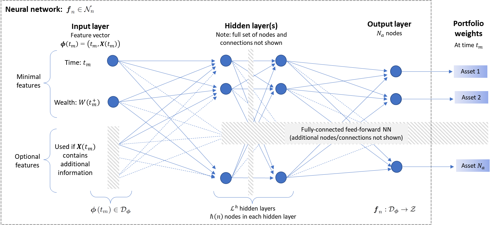
Figure 3.1: Illustration of the structure of the NN as per (3.9). Additional construction and implementation details can be found in Appendix A.

For some fixed value of the index $n\in\mathbb{N}$, let $\mathcal{N}_{n}$ denote the set of NNs constructed in the same way as $\boldsymbol{f}_{n}$ for the fixed and given values of $\mathcal{L}^{h}$ and $\hbar\left(n\right)$. While a formal definition of the set $\mathcal{N}_{n}$ is provided in Appendix A, here we simply note that each NN $\boldsymbol{f}_{n}\left(\cdot;\boldsymbol{\theta}_{n}\right)\in\mathcal{N}_{n}$ only differs in terms of the parameter values constituting its parameter vector $\boldsymbol{\theta}_{n}$ (i.e. for a fixed $n$, each $\boldsymbol{f}_{n}\in\mathcal{N}_{n}$ has the same number of hidden layers $\mathcal{L}^{h}$, hidden nodes $\hbar\left(n\right)$, activation functions etc.).

Observing that $\mathcal{N}_{n}\subset C\left(\mathcal{D}_{\boldsymbol{\phi}},\mathcal{Z}\right)$, our first step is to approximate (3.8) by performing the optimization over $\boldsymbol{f}_{n}\left(\cdot;\boldsymbol{\theta}_{n}\right)\in\mathcal{N}_{n}$ instead. In other words, we approximate the control $\boldsymbol{p}$ by a neural network $\boldsymbol{f}_{n}\in\mathcal{N}_{n}$,

$$\boldsymbol{p}\left(\boldsymbol{\phi}\left(t\right)\right) \simeq \boldsymbol{f}_{n}\left(\boldsymbol{\phi}\left(t\right);\boldsymbol{\theta}_{n}\right),\qquad\textrm{where }\quad\boldsymbol{\phi}\left(t\right)=\left(t,\boldsymbol{X}\left(t\right)\right),\boldsymbol{p}\in C\left(\mathcal{D}_{\boldsymbol{\phi}},\mathcal{Z}\right),\boldsymbol{f}_{n}\in\mathcal{N}_{n}.$$ (3.10)

We identify the NN $\boldsymbol{f}_{n}\left(\cdot;\boldsymbol{\theta}_{n}\right)$ with its parameter vector $\boldsymbol{\theta}_{n}$, so that the (approximate) objective functional using approximation (3.10) is written as

$$J_{n}\left(\boldsymbol{\theta}_{n},\xi;t_{0},w_{0}\right) = E^{t_{0},w_{0}}\left[F\left(W\left(T;\boldsymbol{\theta}_{n},\boldsymbol{Y}\right),\xi\right)+G\left(W\left(T;\boldsymbol{\theta}_{n},\boldsymbol{Y}\right),E^{t_{0},w_{0}}\left[W\left(T;\boldsymbol{\theta}_{n},\boldsymbol{Y}\right)\right],w_{0},\xi\right)\begin{array}[]{c}\!\!\!\!\!\!\!\!\\ \!\!\!\!\!\!\!\!\end{array}\right].$$ (3.13)

Combining (3.9) and (3.10), the wealth dynamics (3.7) is expressed as

$$W\left(t_{m+1}^{-};\boldsymbol{\theta}_{n},\boldsymbol{Y}\right) = \left[W\left(t_{m}^{-};\boldsymbol{\theta}_{n},\boldsymbol{Y}\right)+q\left(t_{m}\right)\right]\cdot\sum_{i=1}^{N_{a}}f_{n,i}\left(\boldsymbol{\phi}\left(t_{m}\right);\boldsymbol{\theta}_{n}\right)\cdot Y_{i}\left(t_{m}\right),\quad m=0,...,N_{rb}-1.$$ (3.14)

Using (3.10) and (3.13), for fixed and given values of $\mathcal{L}^{h}$ and $\hbar\left(n\right)$, we therefore approximate problem (3.8) by

$$V_{n}\left(t_{0},w_{0}\right) = \inf_{\xi\in\mathbb{R}}\inf_{\boldsymbol{f}_{n}\left(\cdot;\boldsymbol{\theta}_{n}\right)\in\mathcal{N}_{n}}J_{n}\left(\boldsymbol{\theta}_{n},\xi;t_{0},w_{0}\right)$$

$$= \inf_{\xi\in\mathbb{R}}\inf_{\boldsymbol{\theta}_{n}\in\mathbb{R}^{\nu_{n}}}J_{n}\left(\boldsymbol{\theta}_{n},\xi;t_{0},w_{0}\right)$$

$$= \inf_{\left(\boldsymbol{\theta}_{n},\xi\right)\in\mathbb{R}^{\nu_{n}+1}}J_{n}\left(\boldsymbol{\theta}_{n},\xi;t_{0},w_{0}\right).$$ (3.16)

We highlight that the optimization in (3.16) is unconstrained since, by construction, each NN $\boldsymbol{f}_{n}\left(\cdot;\boldsymbol{\theta}_{n}\right)\in\mathcal{N}_{n}$ always generates outputs in $\mathcal{Z}$.

The notation $\left(\boldsymbol{\theta}_{n}^{\ast},\xi^{\ast}\right)$ and the associated NN $\boldsymbol{f}_{n}^{\ast}\left(\cdot;\boldsymbol{\theta}_{n}^{\ast}\right)\in\mathcal{N}_{n}$ are subsequently used to denote the values achieving the optimum in (3.16) for given values of $\mathcal{L}^{h}$ and $\hbar\left(n\right)$. Note however that we do not assume that the optimal control $\boldsymbol{p}^{\ast}\in C\left(\mathcal{D}_{\boldsymbol{\phi}},\mathcal{Z}\right)$ satisfying Assumption 3.1 is also a NN in $\mathcal{N}_{n}$, since by the universal approximation results (see for example Hornik et al. (1989)), we would expect that the error in approximating (3.8) by (3.16) can be made arbitrarily small for sufficiently large $\hbar\left(n\right)$. These claims are rigorously confirmed in Section 4 below, where we consider a sequence of NNs $\boldsymbol{f}_{n}\left(\cdot;\boldsymbol{\theta}_{n}\right)\in\mathcal{N}_{n}$ obtained by letting $\hbar\left(n\right)\rightarrow\infty$ as $n\rightarrow\infty$ (for any fixed value of $\mathcal{L}^{h}\geq 1$).

3.2 Step 2 : Computational estimate of the optimal control

In order to solve the approximation (3.16) to problem (3.8), we require estimates of the expectations in (3.13). For computational purposes, suppose we take as given a set $\mathcal{Y}_{n}\in\mathbb{R}^{n\times N_{a}\times N_{rb}}$, consisting of $n\in\mathbb{N}$ independent realizations of the paths of joint asset returns $\boldsymbol{Y}$,

$$\mathcal{Y}_{n} = \left\{\boldsymbol{Y}^{\left(j\right)}:j=1,...,n\right\}.$$ (3.17)

We highlight that each entry $\boldsymbol{Y}^{\left(j\right)}\in\mathcal{Y}_{n}$ consists of a path of joint asset returns (see (2.6)), and we assume that the paths are independent, we do not assume that the asset returns constituting each path are independent. In particular, both cross-correlations and autocorrelation structures within each path of returns are permitted.

Constructing the set $\mathcal{Y}_{n}$ in practical applications is further discussed in Appendix B. In the numerical examples in Section 5, we use examples where $\mathcal{Y}_{n}$ is generated using (i) Monte Carlo simulation of parametric asset dynamics, (ii) stationary block bootstrap resampling of empirical asset returns, (Anarkulova et al. (2022)) and (iii) generative adversarial network (GAN)-generated synthetic asset returns (Yoon et al. (2019)). While we let $n\rightarrow\infty$ in (3.17) for convergence analysis purposes, in practical applications (e.g. the results of Section 5) we simply choose $n$ sufficiently large such that we are reasonably confident that reliable numerical estimates of the expectations in (3.13) are obtained.

Given a NN $\boldsymbol{f}_{n}\left(\cdot;\boldsymbol{\theta}_{n}\right)\in\mathcal{N}_{n}$ and set $\mathcal{Y}_{n}$, the wealth dynamics (3.14) along path $\boldsymbol{Y}^{\left(j\right)}\in\mathcal{Y}_{n}$ is given by

$$W^{\left(j\right)}\left(t_{m+1}^{-};\boldsymbol{\theta}_{n},\mathcal{Y}_{n}\right) = \left[W^{\left(j\right)}\left(t_{m}^{-};\boldsymbol{\theta}_{n},\mathcal{Y}_{n}\right)+q\left(t_{m}\right)\right]\cdot\sum_{i=1}^{N_{a}}f_{n,i}\left(\boldsymbol{\phi}^{\left(j\right)}\left(t_{m}\right);\boldsymbol{\theta}_{n}\right)\cdot Y_{i}^{\left(j\right)}\left(t_{m}\right),$$ (3.18)

for $m=0,...,N_{rb}-1$. We introduce the superscript $\left(j\right)$ to emphasize that the quantities are obtained along the $j$th entry of (3.17).

The computational estimate of $J_{n}\left(\boldsymbol{\theta}_{n},\xi;t_{0},w_{0}\right)$ in (3.13) is then given by

$$\hat{J}_{n}\left(\boldsymbol{\theta}_{n},\xi;t_{0},w_{0},\mathcal{Y}_{n}\right) = \frac{1}{n}\sum_{j=1}^{n}F\left(W^{\left(j\right)}\left(T;\boldsymbol{\theta}_{n},\mathcal{Y}_{n}\right),\xi\right)$$ (3.19)

$$+\frac{1}{n}\sum_{j=1}^{n}G\left(W^{\left(j\right)}\left(T;\boldsymbol{\theta}_{n},\mathcal{Y}_{n}\right),\frac{1}{n}\sum_{k=1}^{n}W^{\left(k\right)}\left(T;\boldsymbol{\theta}_{n},\mathcal{Y}_{n}\right),w_{0},\xi\right),$$

so that we approximate problem (3.16) by

$$\hat{V}_{n}\left(t_{0},w_{0};\mathcal{Y}_{n}\right) = \inf_{\left(\boldsymbol{\theta}_{n},\xi\right)\in\mathbb{R}^{\nu_{n}+1}}\hat{J}_{n}\left(\boldsymbol{\theta}_{n},\xi;t_{0},w_{0},\mathcal{Y}_{n}\right).$$ (3.20)

The numerical solution of (3.20) can then proceed using standard (stochastic) gradient descent techniques (see Appendix B). For subsequent reference, let $\left(\hat{\boldsymbol{\theta}}_{n}^{\ast},\hat{\xi}_{n}^{\ast}\right)$ denote the optimal point in (3.20) relative to the training data set $\mathcal{Y}_{n}$ in (3.20).

In the case of sufficiently large datasets (3.17), in other words as $n\rightarrow\infty$, we would expect that the error in approximating (3.16) by (3.20) can be made arbitrarily small. However, as noted above, as $n\rightarrow\infty$ and the number of hidden nodes $\hbar\left(n\right)\rightarrow\infty$ (for any fixed $\mathcal{L}^{h}\geq 1$), (3.16) is also expected to approximate (3.8) more accurately. As a result, we obtain the necessary intuition for establishing the convergence of (3.20) to (3.8) under suitable conditions, which is indeed confirmed in the results of Section 4.

Note that since $\mathcal{Y}_{n}$ is used in (3.20) to obtain the optimal NN parameter vector $\hat{\boldsymbol{\theta}}_{n}^{\ast}$, it is usually referred to as the NN “training” dataset (see for example Goodfellow et al. (2016)). Naturally, we can also construct a “testing” dataset $\mathcal{Y}_{\hat{n}}^{test}$, that is of a similar structure as (3.17), but typically based on a different implied distribution of $\boldsymbol{Y}$ as a result of different data generation assumptions. For example, $\mathcal{Y}_{\hat{n}}^{test}$ can be obtained using a different time period of historical data for its construction, or different process parameters if there are parametric asset dynamics specified. The resulting approximation $\boldsymbol{f}_{n}^{\ast}\left(\cdot;\hat{\boldsymbol{\theta}}_{n}^{\ast}\right)\in\mathcal{N}_{n}$ to the optimal control $\boldsymbol{p}^{\ast}\in C\left(\mathcal{D}_{\boldsymbol{\phi}},\mathcal{Z}\right)$ obtained using the training dataset in (3.20) can then be implemented on the testing dataset for out-of-sample testing or scenario analysis. This is discussed in more detail in Appendix B.

Remark 3.1.

(Extension to wealth path-dependent objectives) As noted in the Introduction, the NN approach as well as the convergence analysis of Section 4 can be extended to objective functions that depend on the entire wealth path $\left\{W\left(t\right):t\in\mathcal{T}\right\}$ instead of just the terminal wealth $W\left(T\right)$. This is achieved by simply modifying (3.19) appropriately and ensuring the wealth is assessed at the desired intervals using (3.18). ∎

3.3 Advantages of the NN approach

The following observations highlight some advantages of the proposed NN approach:

1. The approach does not rely on dynamic programming (DP) methods for the solution of problem (3.20), and therefore does not require value iteration or backward time stepping. In particular, we observe that due to the explicit time-dependence of the NN feature vector, the optimization problem (3.20) itself only indirectly depends on the number of rebalancing events, while time recursion is limited to the (computationally inexpensive) wealth dynamics (3.18). As result, problems relating to the error amplification associated with DP methods (Wang and Foster (2020); Tsang and Wong (2020); Li et al. (2020)) are avoided, and only a single optimization problem that is independent of the number of portfolio rebalancing events is solved, in contrast to DP-based methods (see for example Bachouch et al. (2022); Van Heeswijk and Poutré (2019)).

   Not relying on DP techniques also makes the approach significantly more flexible, in that it can directly handle objective functions that are not separable in the sense of DP, without requiring theoretical results such as embedding in the case of MV optimization (see for example Zhou and Li (2000); Li and Ng (2000)). As an example of this, we present the solution of the mean - semi-variance problem (2.18) in Section 5.

2. The proposed methodology is parsimonious, in the sense that the NN parameter vector remains independent of number of rebalancing events. Specifically, we observe that the NN parameter vector $\boldsymbol{\theta}_{n}\in\mathbb{R}^{\nu_{n}}$ of the NN does not depend on the rebalancing time $t_{m}\in\mathcal{T}$ or on the sample path $j$. This contrasts our approach with the approaches of for example Han and Weinan (2016); Tsang and Wong (2020), where the number of parameters scale with the number of rebalancing events. As a result, the NN approach presented here can lead to potentially significant computational advantages in the cases of (i) long investment time horizons or (ii) short trading time horizons with a frequent number of portfolio rebalancing events.

   A natural question might be whether the NNs in the proposed approach are required to be very deep, thus potentially exposing the training of the NN in (3.20) to problem of vanishing or exploding gradients (see for example Goodfellow et al. (2016)). However, the ground truth results presented in Section 5 demonstrate that we obtain very accurate results with relatively shallow NNs (at most two hidden layers). We suspect this might be due to the optimal control being relatively low-dimensional compared to the high-dimensional objective functionals in portfolio optimization problems with discrete rebalancing (see Van Staden et al. (2022b) for a rigorous analysis), while in this NN approach approach the optimal control is obtained directly without requiring the solution of the (high-dimensional) objective functional at rebalancing times.

Note that these advantages also contrast the NN approach with Reinforcement Learning-based algorithms to solve portfolio optimization problems, as the following remark discusses.

Remark 3.2.

(Contrast of NN approach to Reinforcement Learning). Reinforcement learning (RL) algorithms (for example, Q-learning) relies fundamentally on the DP principle for the numerical solution of the portfolio optimization problem (see for example Gao et al. (2020); Lucarelli and Borrotti (2020); Park et al. (2020)). This requires, at each value iteration step, the approximation of a (high-dimensional) conditional expectation. As a result, RL is associated with standard DP-related concerns related to error amplification and the curse of dimensionality discussed above, and also cannot solve general problems of the form (1.1) without relying on for example an embedding approach to obtain an associated problem that can be solved using DP methods.∎

4 Convergence analysis

In this section, we present the theoretical justification of the proposed NN approach as outlined in Section 3. We confirm that the numerical solution of (3.20) can be used to approximate the theoretical solution of (3.8) arbitrarily well (in probability) under suitable conditions. This section only summarizes the key convergence results which are among the main contributions of this paper, while additional technical details and proofs are provided in Appendix A.

We start with Theorem 4.1, which confirms the validity of Step 1 (Subsection 3.1), namely using a NN $\boldsymbol{f}_{n}\left(\cdot;\boldsymbol{\theta}_{n}\right)\in\mathcal{N}_{n}$ to approximate the control. Note that Theorem 4.1 relies on two assumptions, presented in Appendix A.2: We emphasize that Assumption A.3 is purely made for purposes of convenience, since its requirements can easily be relaxed with only minor modifications to the proofs (as discussed in Remark A.1), but at the cost of significant notational complexity and no additional insights. In contrast, Assumption A.2 is critical to establish the result of Theorem 4.1, and requires that the optimal investment strategy (or control) satisfies Assumption 3.1, places some basic requirements on $F$ and $G$, and assumes that the sequence of NNs $\left\{\boldsymbol{f}_{n}\left(\cdot;\boldsymbol{\theta}_{n}\right),n\in\mathbb{N}\right\}$ is constructed such that the number of nodes in each hidden layer $\hbar\left(n\right)\rightarrow\infty$ as $n\rightarrow\infty$ (no assumptions are yet required regarding the exact form of $n\rightarrow\hbar\left(n\right)$).

Theorem 4.1.

(Validity of NN approximation) We assume that Assumption A.2 holds, and for ease of exposition, we also assume that Assumption A.3 holds. Then the NN approximation to the control in (3.10) is valid, in the sense that $V\left(t_{0},w_{0}\right)$ in (3.8) can be approximated arbitrarily well by $V_{n}\left(t_{0},w_{0}\right)$ in (3.16) for sufficiently large $n$, since

$$\lim_{n\rightarrow\infty}\left|V_{n}\left(t_{0},w_{0}\right)-V\left(t_{0},w_{0}\right)\right| = \lim_{n\rightarrow\infty}\left|\inf_{\left(\boldsymbol{\theta}_{n},\xi\right)\in\mathbb{R}^{\nu_{n}+1}}J_{n}\left(\boldsymbol{\theta}_{n},\xi;t_{0},w_{0}\right)-\inf_{\xi\in\mathbb{R}}\inf_{\boldsymbol{p}\in C\left(\mathcal{D}_{\boldsymbol{\phi}},\mathcal{Z}\right)}J\left(\boldsymbol{p},\xi;t_{0},w_{0}\right)\right|$$ (4.1)

$$= 0.$$

Proof.

See Appendix A.3. ∎

Having justified Step 1 of the approach, Theorem 4.2 now confirms the validity of Step 2 of the NN approach (see Subsection 3.2), namely using the computational estimate $\boldsymbol{f}_{n}^{\ast}\left(\cdot;\hat{\boldsymbol{\theta}}_{n}^{\ast}\right)\in\mathcal{N}_{n}$ from (3.20) as an approximation of the true optimal control $\boldsymbol{p}^{\ast}\in C\left(\mathcal{D}_{\boldsymbol{\phi}},\mathcal{Z}\right)$. Note that in addition to the assumptions of Theorem 4.1, Theorem 4.2 also requires Assumption A.4, which by necessity includes computational considerations such as the structure of the training dataset $\mathcal{Y}_{n}$, the rate of divergence of the number of hidden nodes $\hbar\left(n\right)\rightarrow\infty$ as $n\rightarrow\infty$, and assumptions regarding the optimization algorithm used in solving problem (3.20).

Theorem 4.2.

(Validity of computational estimate) We assume that Assumption A.2, Assumption A.3 and Assumption A.4 hold. Then the computational estimate to the optimal control (3.2) obtained using (3.10) and (3.20) is valid, in the sense that the value function $V\left(t_{0},w_{0}\right)$ in (3.8) can be approximated arbitrarily well in probability by $\hat{V}_{n}\left(t_{0},w_{0};\mathcal{Y}_{n}\right)$ in (3.20) for sufficiently large $n$, since

$$\left|\hat{V}_{n}\left(t_{0},w_{0};\mathcal{Y}_{n}\right)-V\left(t_{0},w_{0}\right)\right| = \left|\inf_{\left(\boldsymbol{\theta}_{n},\xi\right)\in\mathbb{R}^{\eta_{n}+1}}\hat{J}_{n}\left(\boldsymbol{\theta}_{n},\xi;t_{0},w_{0},\mathcal{Y}_{n}\right)-\inf_{\xi\in\mathbb{R}}\inf_{\boldsymbol{p}\in C\left(\mathcal{D}_{\boldsymbol{\phi}},\mathcal{Z}\right)}J\left(\boldsymbol{p},\xi;t_{0},w_{0}\right)\right|$$ (4.2)

$$\overset{P}{\longrightarrow} 0,\qquad\textrm{as }n\rightarrow\infty.$$

Proof.

See Appendix A.3. ∎

Taken together, Theorem 4.1 and Theorem 4.2 establish the theoretical validity of the NN approach to solve problems of the form (1.1).

5 Numerical results

In this section, we present numerical results obtained by implementing the NN approach described in Section 3. For illustrative purposes, the examples focus on investment objectives as outlined in Subsection 2.1, and we use three different data generation techniques for obtaining the training data set $\mathcal{Y}_{n}$ of the NN: (i) parametric models for underlying asset returns, (ii) stationary block bootstrap resampling of empirical returns, and (ii) generative adversarial network (GAN)-generated synthetic asset returns.

5.1 Closed-form solution: $DSQ\left(\gamma\right)$ with continuous rebalancing

Under certain conditions, some of the optimization problems in Subsection 2.1 can be solved analytically. In this subsection, we demonstrate how a closed-form solution of problem $DSQ\left(\gamma\right)$ in (2.12), assuming continuous rebalancing (i.e. if we let $\Delta t\rightarrow 0$ in (2.1)), can be approximated very accurately using a very simple NN (1 hidden layer, only 3 hidden nodes) using discrete rebalancing with $\Delta t\gg 0$ in (2.1). This simultaneously illustrates how parsimonious the NN approach is, as well as how useful the imposition of time-continuity is in ensuring the smooth behavior of the (approximate) optimal control.

In this subsection as well as in Subsection 5.2, we assume parametric dynamics for the underlying assets. For concreteness, we consider the scenario of two assets, $N_{a}=2$, with unit values $S_{i},i=1,2$, evolving according to the following dynamics,

$$\frac{dS_{i}\left(t\right)}{S_{i}\left(t^{-}\right)} = \left(\mu_{i}-\lambda_{i}\kappa_{i}^{\left(1\right)}\right)\cdot dt+\sigma_{i}\cdot dZ_{i}\left(t\right)+d\left(\sum_{k=1}^{\pi_{i}\left(t\right)}\left(\vartheta_{i}^{\left(k\right)}-1\right)\right),\qquad i=1,2.$$ (5.1)

Note that (5.1) takes the form of the standard jump diffusion models in finance - see e.g. Merton (1976); Kou (2002) for more information. For each asset $i$ in (5.1), $\mu_{i}$ and $\sigma_{i}$ denote the (actual, not risk-neutral) drift and volatility, respectively, $Z_{i}$ denotes a standard Brownian motion, $\pi_{i}\left(t\right)$ denotes a Poisson process with intensity $\lambda_{i}\geq 0$, and $\vartheta_{i}^{\left(k\right)}$ are i.i.d. random variables with the same distribution as $\vartheta_{i}$, which represents the jump multiplier of the $i$th risky asset with $\kappa_{i}^{\left(1\right)}=\mathbb{E}\left[\vartheta_{i}-1\right]$ and $\kappa_{i}^{\left(2\right)}=\mathbb{E}\left[\left(\vartheta_{i}-1\right)^{2}\right]$. While the Brownian motions can be correlated with $dZ_{1}\left(t\right)dZ_{2}\left(t\right)=\rho_{1,2}\cdot dt$, we make the standard assumption that the jump components are independent (see for example Forsyth and Vetzal (2022)).

For this subsection only, we treat the first asset ($i=1$ in (5.1)) as a “risk-free” asset, and set $\mu_{1}=r>0$ where $r$ is the risk-free rate, so that we have $\lambda_{1}=0$, $\sigma_{1j}=0$ $\forall j$, and $Z_{1}\equiv 0$, while the second asset ($i=2$ in (5.1)) is assumed to be a broad equity market index (the “risky asset”). In this scenario, if problem $DSQ\left(\gamma\right)$ in (2.12) is solved subject to dynamics (5.1) together with the assumptions of costless continuous trading, infinite leverage, and uninterrupted trading in the event of insolvency, then the $DSQ\left(\gamma\right)$-optimal control can be obtained analytically as

$$\boldsymbol{p}^{\ast}\left(t,W^{\ast}\left(t\right)\right) =\left[1-p_{2}^{\ast}\left(t,W^{\ast}\left(t\right)\right),p_{2}^{\ast}\left(t,W^{\ast}\left(t\right)\right)\right]\in\mathbb{R}^{2},$$ (5.2)

where the fraction of wealth in the broad stock market index (asset $i=2$) is given by (Zweng and Li (2011))

$$p_{2}^{\ast}\left(t,W^{\ast}\left(t\right)\right) =\frac{\mu_{2}-r}{\sigma_{2}^{2}+\lambda_{2}\kappa_{2}^{\left(2\right)}}\cdot\left[\frac{\gamma e^{-r\left(T-t\right)}-W^{\ast}\left(t\right)}{W^{\ast}\left(t\right)}\right],\qquad w_{0}<\gamma e^{-r\left(T-t\right)}.$$ (5.3)

By design, the NN approach is not constructed to solve problems with unrealistic assumptions such as continuous trading, infinite leverage and short-selling, or trading in the event of bankruptcy, all of which are required to derive (5.3). However, if the implicit quadratic wealth target for the DSQ problem (i.e. the value of $\gamma$, see Vigna (2014)) is not too aggressive, the analytical solution (5.3) does not require significant leverage or lead to a large probability of insolvency. In such a scenario, we can use the NN approach to approximate (5.3).

We select $w_{0}=100$, $T=1$ year and $\gamma=138.33$, and simulate $n=2.56\times 10^{6}$ paths of the underlying assets using (5.1) and parameters as in Table C.1 (Appendix C). On this set of paths, the true analytical solution (5.3) is implemented using 7,200 time steps. In contrast, for the NN approach, we use only 4 rebalancing events in $\left[0,T=1\right]$, and therefore aggregate the simulated returns in quarterly time intervals to construct the training data set $\mathcal{Y}_{n}$. We consider only a very shallow NN, consisting of a single hidden layer and only 3 hidden nodes.

Figure 5.1 compares the resulting optimal investment strategies by illustrating the optimal proportion of wealth invested in the the broad equity market index (asset $i=2$) as a function of time and wealth. We emphasize that the NN strategy in Figure 5.1(b) is not expected to be exactly identical to the analytical solution in Figure 5.1(a), since it is based on fundamentally different assumptions such as discrete rebalancing and investment constraints (2.5).

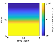
(a) Closed-form solution, $\Delta t\rightarrow 0$ ($w_{0}\in\mathbb{R}$)

      

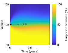
(b) Shallow NN, $\Delta t=0.25$ ($w_{0}=100$)

Figure 5.1: Closed-form solution - $DSQ\left(\gamma\right)$ with continuous rebalancing: Optimal proportion of wealth invested in the broad equity market index as a function of time and wealth. The NN approximation is obtained for a specific initial wealth of $w_{0}=$100, and only four rebalancing events in $\left[0,T\right]$.

However, requiring that the NN feature vector includes time in the proposed NN approach, together with a NN parameter vector that does not depend on time, we guarantee the smooth behavior in time of the NN approximation observed in Figure 5.1(b). As a result, Table 5.1 shows that the shallow NN strategy trained with $\Delta t\gg 0$ results in a remarkably accurate and parsimonious approximation to the true analytical solution where $\Delta t\rightarrow 0$, since we obtain nearly identical optimal terminal wealth distributions.

Table 5.1: Closed-form solution - $DSQ\left(\gamma\right)$ with continuous rebalancing: Percentiles of the simulated ( $n=2.56\times 10^{6}$) terminal wealth distributions obtained by implementing the optimal strategies in Figure 5.1. In both cases, a mean terminal wealth of 105 is obtained. Note that the NN approximation was obtained under the assumption of quarterly rebalancing only, no leverage or short-selling, and therefore no trading in insolvency.

		$W\left(T\right)$ percentiles
Solution approach	Rebalancing	5th	20th	50th	80th	95th
Closed-form solution	Continuous, $\Delta t$$\rightarrow 0$	86.81	98.02	106.35	112.82	118.15
Shallow NN approximation	Discrete, $\Delta t=0.25$, total of $N_{rb}=4$ only	86.62	97.30	105.67	112.54	118.85

5.2 Ground truth: Problem $MCV\left(\rho\right)$

In the case of the Mean-CVaR problem $MCV\left(\rho\right)$ in (2.17), Forsyth and Vetzal (2022) obtain an MCV-optimal investment strategy subject to the same investment constraints as in Section 2 (namely discrete rebalancing, no short-selling or leverage allowed, and no trading in insolvency) using the partial (integro-)differential equation (PDE) approach of Forsyth (2020).

For ground truth analysis purposes, we therefore consider the same investment scenario as in Forsyth and Vetzal (2022), where two underlying assets are considered, namely 30-day US T-bills and a broad equity market index (the CRSP VWD index) - see Appendix C for definitions. However, in contrast to the preceding section where one asset was taken as the risk-free asset, both assets are now assumed to evolve according to dynamics of the form (5.1), using the double-exponential Kou (2002) formulation for the jump distributions. The NN training data set is therefore constructed by simulating the same underlying dynamics. While further details regarding the context and motivation for the investment scenario can be found in Forsyth and Vetzal (2022), here we simply note that the scenario involves $T=5$ years, quarterly rebalancing, a set of admissible strategies satisfying (2.5), and parameters for (5.1) as in Table C.2.

As discussed in Appendix B, the inherently higher complexity of the Mean-CVaR optimal control requires the NN to be deeper than in the case of the problem considered in Subsection 5.1. As a result, we consider approximating NNs with two hidden layers, each with 8 hidden nodes, while relatively large mini-batches of 2,000 paths were used in the stochastic gradient descent algorithm (see Appendix B) to ensure sufficiently accurate sampling of the tail of the returns distribution in selecting the descent direction at each step. Note that despite using a deeper NN, this NN structure is still very parsimonious and relatively shallow compared to the rebalancing time-dependent structures considered in for example Han and Weinan (2016), where a new set of parameters is introduced at each rebalancing event.

Table 5.2 compares the PDE results reported in Forsyth and Vetzal (2022) with the corresponding NN results. Note that the PDE optimal control was determined by solving a Hamilton-Jacobi-Bellman PDE numerically. The statistics for the PDE generated control were computed using $n=2.56\times 10^{6}$ Monte Carlo simulations of the joint underlying asset dynamics in order to calculate the results of Table 5.2, while the NN was trained on $n=2.56\times 10^{6}$ paths of the same underlying asset dynamics but which were independently simulated. While some variability of the results are therefore to be expected due to the underlying samples, the results in Table 5.2 demonstrate the robustness of the proposed NN approach.

Table 5.2: Ground truth - problem $MCV\left(\rho\right)$: The PDE results are obtained from Forsyth and Vetzal (2022) for selected points on the Mean-CVaR “efficient frontier”. The “Value function” column reports the value of the objective function (2.16) under the corresponding optimal control, while “% difference” reports the percentage difference in the reported value functions for the NN solution compared to the PDE solution.

$\rho$	5% CVaR		$E^{t_{0},w_{0}}\left[W\left(T\right)\right]$		Value function		% difference
	PDE	NN	PDE	NN	PDE	NN
0.10	940.60	940.55	1069.19	1062.97	1047.52	1046.85	-0.06%
0.25	936.23	937.39	1090.89	1081.99	1208.95	1207.88	-0.09%
1.00	697.56	690.11	1437.73	1444.16	2135.29	2134.27	-0.05%
1.50	614.92	611.65	1508.10	1510.07	2877.07	2876.76	-0.01%

5.3 Ground truth: Problems $MV\left(\rho\right)$ and $DSQ\left(\gamma\right)$

In this subsection, we demonstrate that if the investment objective (1.1) is separable in the sense of dynamic programming, the correct time-consistent optimal investment strategy is recovered, otherwise we obtain the correct pre-commitment (time-inconsistent) investment strategy.

To demonstrate this, the theoretical embedding result of Li and Ng (2000); Zhou and Li (2000), which establishes the equivalence of problems $MV\left(\rho\right)$ and $DSQ\left(\gamma\right)$ under fairly general conditions, can be exploited for ground truth analysis purposes as follows. Suppose we solved problems $MV\left(\rho\right)$ and $DSQ\left(\gamma\right)$ on the same underlying training data set. We remind the reader that in the proposed NN approach, problem $MV\left(\rho\right)$ can indeed be solved directly without difficulty, which is not possible in dynamic programming-based approaches. Then, considering the numerical results, there should be values of parameters $\rho\equiv\tilde{\rho}$ and $\gamma\equiv\tilde{\gamma}$ such that the optimal strategy of $MV\left(\rho\equiv\tilde{\rho}\right)$ corresponds exactly to the optimal strategy of $DSQ\left(\gamma\equiv\tilde{\gamma}\right)$, with a specific relationship holding between $\tilde{\rho}$ and $\tilde{\gamma}$. The NN approach can therefore enable us to numerically demonstrate the embedding result of Li and Ng (2000); Zhou and Li (2000) in a setting where the underlying asset dynamics are not explicitly specified and where multiple investment constraints are present. We start by recalling the embedding result.

Proposition 5.1.

(Embedding result of Li and Ng (2000); Zhou and Li (2000)) Fix a value $\tilde{\rho}>0$. If $\mathcal{P}^{\ast}\in\mathcal{A}$ is the optimal control of problem $MV\left(\rho\equiv\tilde{\rho}\right)$ in (2.14), then $\mathcal{P}^{\ast}$ is also the optimal control for problem $DSQ\left(\gamma=\tilde{\gamma}\right)$ in (2.12), provided that

$$\tilde{\gamma} = \frac{1}{2\tilde{\rho}}+E^{t_{0},w_{0}}\left[W^{\ast}\left(T;\mathcal{P}^{\ast},\boldsymbol{Y}\right)\right].$$ (5.4)

Proof.

See Li and Ng (2000); Zhou and Li (2000). We also highlight the alternative proof provided in Dang and Forsyth (2016), which shows that this result is valid for any admissible control set $\mathcal{A}$. ∎

Since (5.4) is valid for any admissible control set $\mathcal{A}$, we consider a factor investing scenario where portfolios are constructed using popular long-only investable equity factor indices (Momentum, Value, Low Volatility, Size), a broad equity market index (the CRSP VWD index), 30-day T-bills and 10-year Treasury bonds (see Appendix C for definitions). For illustrative purposes in the case of an investor primarily concerned with long-run factor portfolio performance, we use a horizon of $T=10$ years, $w_{0}=120$, annual contributions of $q\left(t_{m}\right)=12$, and annual rebalancing.

Given historical returns data for the underlying assets, we construct training and testing (out-of-sample) data sets for the NN, $\mathcal{Y}_{n}$ and $\mathcal{Y}_{\hat{n}}^{test}$, respectively, using stationary block bootstrap resampling of empirical historical asset returns (see Appendix C), which is popular with practitioners (Anarkulova et al. (2022); Cogneau and Zakalmouline (2013); Dichtl et al. (2016); Scott and Cavaglia (2017); Cavaglia et al. (2022); Simonian and Martirosyan (2022)) and is designed to handle weakly stationary time series with serial dependence. See Ni et al. (2022) for a discussion concerning the probability of obtaining a repeated path in block bootstrap resampling (which is negligible for any realistic number of samples). Due to availability of historical data we use inflation-adjusted monthly empirical returns from 1963:07 to 2020:12. The training data set ($n=10^{6}$) is obtained using an expected block size of 6 months of joint returns from 1963:07 to 2009:12, while the testing data set ($n=10^{6}$) uses an expected block size of 3 months and returns from 2010:01 to 2020:12. We consider NNs with two hidden layers, each with only eight hidden nodes.

Choosing two values of $\tilde{\rho}>0$ to illustrate different levels of risk aversion (see Table 5.3), we solve problem $MV\left(\rho=\tilde{\rho}\right)$ in (2.14) directly using the proposed approach to obtain the optimal investment strategy $\boldsymbol{f}\left(\cdot;\hat{\boldsymbol{\theta}}_{mv}^{\ast}\right)$. Note that since we consider a fixed NN structure in this setting rather than a sequence of NNs, we drop the subscript “$n$” in the notation $\boldsymbol{f}\left(\cdot;\hat{\boldsymbol{\theta}}_{mv}^{\ast}\right)$. Using this result together with (5.4), we can approximate the associated value of $\tilde{\gamma}$ by

$$\tilde{\gamma} \simeq \frac{1}{2\tilde{\rho}}+\frac{1}{n}\sum_{j=1}^{n}W^{\ast\left(j\right)}\left(T;\hat{\boldsymbol{\theta}}_{mv}^{\ast},,\mathcal{Y}_{n}\right),$$ (5.5)

and solve problem $DSQ\left(\gamma=\tilde{\gamma}\right)$ independently using the proposed approach on the same training data set $\mathcal{Y}_{n}$.

According to Proposition 5.1, the resulting investment strategy $\boldsymbol{f}\left(\cdot;\hat{\boldsymbol{\theta}}_{dsq}^{\ast}\right)$ should be (approximately) identical to the strategy $\boldsymbol{f}\left(\cdot;\hat{\boldsymbol{\theta}}_{mv}^{\ast}\right)$ if the proposed approach works as required. Note that the parameter vectors are expected to be different (i.e. $\hat{\boldsymbol{\theta}}_{dsq}^{\ast}\neq\hat{\boldsymbol{\theta}}_{mv}^{\ast}$) due to a variety of reasons (multiple local minima, optimization using SGD, etc.), but the resulting wealth distributions and asset allocation should agree, i.e. $\boldsymbol{f}\left(\cdot;\hat{\boldsymbol{\theta}}_{dsq}^{\ast}\right)\simeq\boldsymbol{f}\left(\cdot;\hat{\boldsymbol{\theta}}_{mv}^{\ast}\right)$.

Figure 5.2 demonstrates the investment strategies $\boldsymbol{f}\left(\cdot;\hat{\boldsymbol{\theta}}_{mv}^{\ast}\right)$ and $\boldsymbol{f}\left(\cdot;\hat{\boldsymbol{\theta}}_{dsq}^{\ast}\right)$ obtained by training the NNs on the same training data set using values of $\tilde{\rho}=0.017$ and $\tilde{\gamma}=429.647$, respectively. Note that the values $\tilde{\rho}$ and $\tilde{\gamma}$ are rounded to three decimal places, and Figure 5.2 corresponds to Results set 1 in Table 5.3. In this example, only four of the underlying candidate assets have non-zero investments, which is to be expected due to the high correlation between long-only equity factor indices.

(a) $MV\left(\rho=\tilde{\rho}\right)$ - Momentum

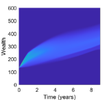
(b) $MV\left(\rho=\tilde{\rho}\right)$ - Value

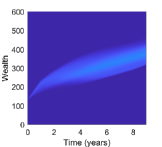
(c) $MV\left(\rho=\tilde{\rho}\right)$ - B10

(d) $MV\left(\rho=\tilde{\rho}\right)$ - T30

(e) $DSQ\left(\gamma=\tilde{\gamma}\right)$ - Momentum

(f) $DSQ\left(\gamma=\tilde{\gamma}\right)$ - Value

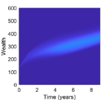
(g) $DSQ\left(\gamma=\tilde{\gamma}\right)$ - B10

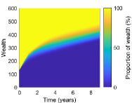
(h) $DSQ\left(\gamma=\tilde{\gamma}\right)$ - T30

Figure 5.2: Ground truth - problems $MV\left(\rho=\tilde{\rho}\right)$ and $DSQ\left(\gamma=\tilde{\gamma}\right)$: investment strategies $\boldsymbol{f}\left(\cdot;\hat{\boldsymbol{\theta}}_{mv}^{\ast}\right)$ and $\boldsymbol{f}\left(\cdot;\hat{\boldsymbol{\theta}}_{dsq}^{\ast}\right)$ obtained by training the NNs using values of $\tilde{\rho}=0.017$ and $\tilde{\gamma}=429.647$ (rounded to three decimal places), respectively. Each figure shows the proportion of wealth invested in the asset as a function of the minimal NN features, namely time and available wealth. Zero investment under the optimal strategies in the broad market index and the Size factor.

Table 5.3 confirms that the associated optimal terminal wealth distributions of $MV\left(\rho=\tilde{\rho}\right)$ and $DSQ\left(\gamma=\tilde{\gamma}\right)$ indeed correspond, both in-sample (training data set) and out-of-sample (testing data set).

Table 5.3: Ground truth - problems $MV\left(\rho=\tilde{\rho}\right)$ and $DSQ\left(\gamma=\tilde{\gamma}\right)$: Terminal wealth results obtained using $n=10^{6}$ joint paths for the underlying assets. Note that the values of $\tilde{\rho}$ and $\tilde{\gamma}$ are rounded to three decimal places, .

	Results set 1: $\tilde{\rho}=0.017$, $\tilde{\gamma}=429.647$				Results set 2: $\tilde{\rho}=0.0097$, $\tilde{\gamma}=493.196$
$W\left(T\right)$	Training data		Testing data		Training data		Testing data
distribution	MV	DSQ	MV	DSQ	MV	DSQ	MV	DSQ
Mean	400.2	400.3	391.2	391.6	441.5	441.8	441.8	441.5
Stdev	55.4	55.4	26.2	25.7	79.6	79.7	39.4	39.5
5th percentile	276.5	276.4	346.6	347.5	255.2	254.6	367.8	367.1
25th percentile	391.8	392.3	382.4	382.8	422.4	423.6	430.9	430.7
50th percentile	416.1	416.3	396.5	396.8	469.8	470.1	451.3	451.2
75th percentile	429.9	429.8	406.4	406.7	487.7	489.6	465.0	464.8
95th percentile	452.1	452.1	418.9	419.0	516.1	516.5	480.9	480.2

The proposed NN approach therefore clearly works as expected, in that we demonstrated that the result of Proposition 5.1 in a completely model-independent way in a portfolio optimization setting where no known analytical solutions exist. In particular, we emphasize that no assumptions were made regarding parametric underlying asset dynamics, the results are entirely data-driven. As a result, we can interpret the preceding results as showing that the approach correctly recovers the time-inconsistent (or pre-commitment) strategy without difficulty if the objective is not separable in the sense of dynamic programming, such as in the case of the $MV\left(\rho\right)$ problem, whereas if the objective is separable in the sense of dynamic programming, such as in the case of the $DSQ\left(\gamma\right)$ problem, the approach correctly recovers the associated time-consistent strategy.

5.4 Mean - Semi-variance strategies

Having demonstrated the reliability of the results obtained using the proposed NN approach with the preceding ground truth analyses, we now consider the solution of the Mean - Semi-variance problem (2.18). To provide the necessary context to interpret the $MSemiV\left(\rho\right)$-optimal results, we compare the results of the optimal solutions of the $MCV\left(\rho=\rho_{mcv}\right)$, $MSemiV\left(\rho=\rho_{msv}\right)$, and $OSQ\left(\gamma=\gamma_{osq}\right)$ problems, where the values of $\rho_{mcv}$, $\rho_{msv}$ and $\gamma_{osq}$ are selected to obtain the same expected value of terminal wealth on the NN training data set. This is done since the MCV- and OSQ-optimal strategies have been analyzed in great detail (Dang and Forsyth (2016); Forsyth (2020)), and are therefore well understood. Note that since all three strategies are related to the maximization of the mean terminal wealth and while simultaneously minimizing some risk measure (which is implicitly done in the case of the OSQ problem, see Dang and Forsyth (2016)), it is natural to compare the strategies on the basis of equal expectation of terminal wealth.

To highlight the main qualitative features of the $MSemiV\left(\rho\right)$-optimal results, we consider a simple investment scenario of two assets, namely 30-day T-bills and a broad equity market index (the VWD index) - see Appendix C for definitions. We choose $T=$5 years, $w_{0}=1000$, and zero contributions to demonstrate a lump sum investment scenario with quarterly rebalancing.

To illustrate the flexibility of the NN approach to underlying data generating assumptions, the NN training data sets are constructed using generative adversarial network (GAN)-generated synthetic asset returns obtained by implementing the TimeGAN algorithm proposed by Yoon et al. (2019). In more detail, using empirical monthly asset returns from 1926:01 to 2019:12 for the underlying assets (data sources are specified in Appendix C), the TimeGAN is trained with default parameters as in Yoon et al. (2019) using block sizes of 6 months to capture both correlation and serial correlation aspects of the (joint) time series. Once trained, the TimeGAN is then used to generate a set of $n=10^{6}$ paths of synthetic asset returns, which is used as the training data set to train the NNs corresponding to the MCV, MSemiV and OSQ-optimal investment strategies.

Figure 5.3 illustrates the resulting optimal investment strategies, and we observe that the MSemiV-optimal strategy is fundamentally different from the MCV and OSQ-optimal strategies, while featuring elements of both. Specifically, Figure 5.4, which illustrates the resulting optimal terminal wealth distributions (with the same expectation), demonstrates that the MSemiV strategy, like the MCV strategy, can offer better downside protection than the OSQ strategy, while the MSemiV strategy retains some of the qualitative elements of the OSQ distribution such as the left skew.

Having illustrated that the MSemiV problem can be solved in a dynamic trading setting using the proposed NN approach to obtain investment strategies that offer potentially valuable characteristics, we leave a more in-depth investigation of the properties and applications of MSemiV-optimal strategies for future work.

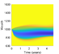
(a) $MCV\left(\rho=\rho_{mcv}\right)$

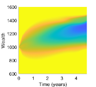
(b) $MSemiV\left(\rho=\rho_{msv}\right)$

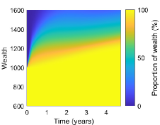
(c) $OSQ\left(\gamma=\gamma_{osq}\right)$

Figure 5.3: Optimal investment strategies for the $MCV\left(\rho=\rho_{mcv}\right)$, $MSemiV\left(\rho=\rho_{msv}\right)$, and $OSQ\left(\gamma=\gamma_{osq}\right)$ strategies, obtaining identical expectation of terminal wealth on the training data set. Each figure shows the proportion of wealth invested in the broad equity market index as a function of the minimal NN features, namely time and available wealth.

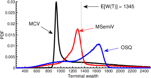
(a) PDFs of $W^{\ast}\left(T\right)$

      

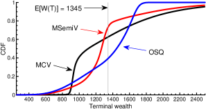
(b) CDFs of $W^{\ast}\left(T\right)$

Figure 5.4: PDFs and CDFs of optimal terminal wealth obtained under the $MCV\left(\rho=\rho_{mcv}\right)$, $MSemiV\left(\rho=\rho_{msv}\right)$, and $OSQ\left(\gamma=\gamma_{osq}\right)$ strategies, where the values of $\rho_{mcv}$, $\rho_{msv}$ and $\gamma_{osq}$ are selected to obtain the same expected value of optimal terminal wealth on the NN training data set.

6 Conclusion

In this paper, we presented a flexible NN approach, which does not rely on dynamic programming techniques, to solve a large class of dynamic portfolio optimization problems. In the proposed approach, a single optimization problem is solved, issues of instability and error propagation involved in estimating high-dimensional conditional expectations are avoided, and the resulting NN is parsimonious in the sense that the number of parameters does not scale with the number of rebalancing events.

We also presented theoretical convergence analysis results which show that the numerical solution obtained using the proposed approach can recover the optimal investment strategy, provided it exists, regardless of whether the resulting optimal investment strategy is time-consistent or (formally) time-inconsistent.

Numerical results confirmed the advantages of the NN approach, and showed that accurate results can be obtained in ground truth analyses in a variety of settings. The numerical results also highlighted that the approach remains agnostic as to the underlying data generating assumptions, so that for example empirical asset returns or synthetic asset returns can be used without difficulty.

We conclude by noting that the NN approach is not necessarily limited to portfolio optimization problems such a those encountered during the accumulation phase of pension funds, and could be extended to address the significantly more challenging problems encountered during the decumulation phase of defined contribution pension funds (see for example Forsyth (2022)). We leave this extension for future work.

7 Declarations

The authors have no competing interests to declare that are relevant to the content of this article. P.A. Forsyth’s work was supported by the Natural Sciences and Engineering Research Council of Canada (NSERC) grant RGPIN-2017-03760.

Appendix A NN approach: technical details and analytical results

In this appendix, additional analytical results, relating to the convergence analysis presented in Section 4, are presented.

A.1 NN structural assumptions

In this section, we discuss the NN structural assumptions. First, we introduce the necessary notation - for a more detailed treatment of NNs, see for example Goodfellow et al. (2016). Consider a fully-connected, feed-forward NN $\boldsymbol{f}_{n}$ with $\mathcal{L}^{h}\geq 1$ hidden layers. The NN layers are indexed by $\ell\in\left\{0,...,\mathcal{L}\right\}$, where $\ell=0$ and $\ell=\mathcal{L}^{h}+1\equiv\mathcal{L}$ denote the input and output layers, respectively. Let $\eta_{n,\ell}\in\mathbb{N}$ denote the number of nodes in layer $\ell$ of $\boldsymbol{f}_{n}$. With the exception of the input layer, each layer $\ell\in\left\{1,...,\mathcal{L}\right\}$ is associated with a weights matrix $\boldsymbol{x}_{n}^{\left[\ell\right]}\in\mathbb{R}^{\eta_{n,\ell}\times\eta_{n,\ell-1}}$ into the layer, an optional bias vector $\boldsymbol{b}_{n}^{\left[\ell\right]}\in\mathbb{R}^{\eta_{n,\ell}}$, as well as an activation function $\boldsymbol{\mathfrak{a}}_{n}^{\left[\ell\right]}:\mathbb{R}^{\eta_{\ell}}\rightarrow\mathbb{R}^{\eta_{\ell}}$ which is applied to the weighted inputs into the layer.

The parameter vector of the NN $\boldsymbol{f}_{n}$, which consists of all weights and biases, is denoted by $\boldsymbol{\theta}_{n}\in\mathbb{R}^{\nu_{n}}$, where $\nu_{n}\in\mathbb{N}$ denotes the total number of weights and biases. In other words, the weights matrices $\left\{\boldsymbol{x}_{n}^{\left[\ell\right]}:\ell=1,...,\mathcal{L}\right\}$ and optional bias vectors $\left\{\boldsymbol{b}_{n}^{\left[\ell\right]}:\ell=1,...,\mathcal{L}\right\}$ are transformed into a single vector $\boldsymbol{\theta}_{n}=\left(\theta_{1},...,\theta_{\nu_{n}}\right)$, where each $\theta_{n,i}\in\boldsymbol{\theta}_{n}$ can be uniquely mapped to a single weight or bias in some layer.

Note that no activation function is applied at the input layer ($\ell=0$), so that the $\eta_{0}\equiv\eta_{n,0}$ output values of the input layer corresponds to feature (input) vector of the NN, which will be denoted by $\boldsymbol{\phi}\in\mathbb{R}^{\eta_{0}}$. Recalling that $\eta_{\mathcal{L}}\equiv\eta_{n,\mathcal{L}}$ is the number of nodes in the output layer ($\ell=\mathcal{L}$) and setting the bias vectors $\boldsymbol{b}_{n}^{\left[\ell\right]}\equiv\boldsymbol{0}$ for convenience, the NN can therefore be written as a single function $\boldsymbol{f}_{n}\left(\boldsymbol{\phi};\boldsymbol{\theta}_{n}\right):\mathbb{R}^{\eta_{0}}\rightarrow\mathbb{R}^{\eta_{\mathcal{L}}}$, where

$$\boldsymbol{f}_{n}\left(\boldsymbol{\phi};\boldsymbol{\theta}_{n}\right) \coloneqq \left(f_{n,1}\left(\boldsymbol{\phi};\boldsymbol{\theta}_{n}\right),...,f_{n,\eta_{\mathcal{L}}}\left(\boldsymbol{\phi};\boldsymbol{\theta}_{n}\right)\right),\qquad\boldsymbol{\phi}\in\mathbb{R}^{\eta_{0}},\boldsymbol{\theta}_{n}\in\mathbb{R}^{\nu_{n}}$$ (A.1)

We highlight that the output of the $i$th node in the output layer is given by $f_{n,i}\left(\boldsymbol{\phi};\boldsymbol{\theta}_{n}\right)=\mathfrak{a}_{n,i}^{\left[\mathcal{L}\right]}$.

Given this standard fully-connected, feedforward NN formulation, we introduce the following NN structural assumption.

Assumption A.1.

(NN structure) Let $\boldsymbol{f}_{n}\left(\cdot;\boldsymbol{\theta}_{n}\right),n\in\mathbb{N}$, be a sequence of fully-connected feedforward neural networks, and let $\hbar\left(n\right),n\in\mathbb{N}$ be a monotonically increasing sequence (i.e. $\hbar\left(n\right)<\hbar\left(n+1\right)$, $\forall n\in\mathbb{N}$) such that $\lim_{n\rightarrow\infty}\hbar\left(n\right)=\infty$. For each $n\in\mathbb{N}$, the NN $\boldsymbol{f}_{n}$ is constructed to satisfy the following structural assumptions.

1. The number of hidden layers $\mathcal{L}^{h}\geq 1$ ($\mathcal{L}^{h}\in\mathbb{N}$) remains fixed for all $n\in\mathbb{N}$. For notational simplicity, we assume that each of the $\mathcal{L}^{h}$ hidden layers of the NN $\boldsymbol{f}_{n}$ has the same number $\hbar\left(n\right)$ of hidden nodes,

   $$\eta_{n,\ell} \equiv \hbar\left(n\right),\qquad\forall\ell=1,...,\mathcal{L}-1,\quad\textrm{ for some }\hbar\left(n\right)\in\mathbb{N}.$$ (A.2)

2. For convenience, we assume that the sigmoid activation function $\sigma^{h}$ is applied at each hidden node,

   $$\sigma^{h}\left(y\right)=\frac{1}{1+e^{-y}} \equiv \mathfrak{a}_{n,i}^{\left[\ell\right]}\left(y\right),\quad\textrm{where }y=\left(\sum_{k=1}^{\eta_{n,\ell-1}}x_{n,ik}^{\left[\ell\right]}\mathfrak{a}_{n,k}^{\left[\ell-1\right]}\right)+b_{n,i}^{\left[\ell\right]},$$ (A.3)

   for all $\ell=1,...,\mathcal{L}^{h}$ and $i=1,...,\hbar\left(n\right)$. Note that in principle, any of the popular activation functions can be used instead of (A.3), with minor modifications to the theoretical analysis presented in this paper.

3. The NN $\boldsymbol{f}_{n}$ has $\eta_{0}=\eta_{X}+1\equiv\eta_{n,0}$ input nodes (i.e. the number of input nodes are independent of $n\in\mathbb{N}$), with feature (input) vectors $\boldsymbol{\phi}\in\mathbb{R}^{\eta_{0}}$ of the form

   $$\boldsymbol{\phi}\coloneqq\boldsymbol{\phi}\left(t\right) \coloneqq \left(t,\boldsymbol{X}\left(t\right)\right)\in\mathcal{D}_{\boldsymbol{\phi}}\subseteq\mathbb{R}^{\eta_{X}+1},\qquad\textrm{with }\boldsymbol{X}\left(t\right)=\left(W\left(t^{+}\right),\hat{\boldsymbol{X}}\left(t\right)\right),$$ (A.4)

   where $W\left(t^{+}\right)$ denotes the wealth available for investment at time $t$ after any contributions to the portfolio at time $t$, while $\hat{\boldsymbol{X}}\left(t\right)$ denotes a vector of additional information taken into account by the investment strategy. We emphasize that (A.4) clarifies that at time $t\in\left[t_{0},T\right]$, at least time $t$ itself and $W\left(t^{+}\right)$ are always assumed to be inputs into the NN.

4. The NN $\boldsymbol{f}_{n}$ has $N_{a}=\eta_{n,\mathcal{L}}$ output nodes (i.e. the number of output nodes are independent of $n\in\mathbb{N}$), with the output of node $i$, denoted by $f_{n,i}\left(\boldsymbol{\phi}\left(t\right);\boldsymbol{\theta}_{n}\right)$, being associated with the proportion of available wealth $W\left(t^{+}\right)$ invested in asset $i\in\left\{1,...,N_{a}\right\}$ after rebalancing the portfolio at time $t$.

5. The output layer ($\ell=\mathcal{L}=\mathcal{L}^{h}+1$) of each NN $\boldsymbol{f}_{n}$ uses the softmax activation function (see for example Gao and Pavel (2018)). Therefore we have $\boldsymbol{\mathfrak{a}}_{n}^{\left[\mathcal{L}\right]}=\boldsymbol{\psi}:\mathbb{R}^{N_{a}}\rightarrow\mathbb{R}^{N_{a}}$, where the $i$th component of $\boldsymbol{\psi}=\left(\psi_{i}:i=1,..,N_{a}\right)$ is given by

   $$\psi_{i}=\mathfrak{a}_{n,i}^{\left[\mathcal{L}\right]}=\frac{\exp\left\{z_{n,i}^{\left[\mathcal{L}\right]}\right\}}{\sum_{m=1}^{N_{a}}\exp\left\{z_{n,m}^{\left[\mathcal{L}\right]}\right\}},\quad\textrm{where }z_{n,i}^{\left[\mathcal{L}\right]}=\sum_{k=1}^{N_{a}}x_{n,ik}^{\left[\mathcal{L}\right]}\mathfrak{a}_{n,k}^{\left[\mathcal{L}-1\right]}+b_{n,i}^{\left[\mathcal{L}\right]},\quad i=1,...,N_{a}.$$ (A.5)

For a given $n\in\mathbb{N}$, we define the set $\mathcal{N}_{n}$ as the set of all neural networks satisfying Assumption (A.1),

$$\mathcal{N}_{n}=\left\{\left.\boldsymbol{f}_{n}:\mathcal{D}_{\boldsymbol{\phi}}\rightarrow\mathcal{Z}\right|\boldsymbol{f}_{n}\left(\cdot;\boldsymbol{\theta}_{n}\right)\textrm{ satisfies Assumption }\ref{assu: Appendix NN structure assumptions}\textrm{ with }\hbar\left(n\right)\textrm{ nodes in each hidden layer}\right\}.$$ (A.6)

In other words, each $\boldsymbol{f}_{n}\left(\cdot;\boldsymbol{\theta}_{n}\right)\in\mathcal{N}_{n}$ has the same number of hidden nodes $\hbar\left(n\right)$ in each hidden layer, but a potentially different parameter vector $\boldsymbol{\theta}_{n}$ (i.e. different values associated with the weights and biases).

We make the following observations regarding Assumption A.1:

• Any NN constructed to satisfy Assumption A.1 will, for any input vector $\boldsymbol{\phi}\left(t\right)$, automatically generate an output in the set $\mathcal{Z}$, hence the definition (A.6) noting that $\boldsymbol{f}_{n}:\mathcal{D}_{\boldsymbol{\phi}}\rightarrow\mathcal{Z}$. In other words, the given constraints are automatically satisfied. However, different sets of constraints simply requires modifications to the output activation, or post-processing of NN outputs, without affecting the technical results.

• Note that further assumptions regarding the rate of at which the sequence $\hbar\left(n\right)$ increases relative to that of the sequence $\left\{n\right\}_{n\in\mathbb{N}}$ will be introduced in the convergence analysis of Section 4 (see Assumption A.4.

• In practical applications, it is not necessary to consider a sequence of NNs; instead, we will use a single NN $\boldsymbol{f}_{\tilde{n}}$ with $\hbar\left(\tilde{n}\right)$ hidden nodes in each of the hidden layers to get a reasonable trade-off between accuracy and computational efficiency. However, we emphasize that any such $\boldsymbol{f}_{\tilde{n}}$ is still constructed to satisfy Assumption A.1.

A.2 Assumptions for convergence analysis

Assumption A.2 introduces the main assumptions used in rigorously justifying the approximation (3.10) and therefore to prove Theorem 4.1.

Assumption A.2.

(Convergence analysis: NN approximation to control) To establish the validity of the NN approximation to the control, we make the following assumptions:

1. The optimal investment strategy (or control) satisfies Assumption 3.1.

2. The functions $F$ and $G$ in the objective functional $J\left(\boldsymbol{p},\xi;t_{0},w_{0}\right)$ (see (3.6)) are continuous, and $\xi\rightarrow F\left(\cdot,\xi\right)$ and $\xi\rightarrow G\left(\cdot,\cdot,\cdot,\xi\right)$ are convex for any admissible strategy $\boldsymbol{p}\in C\left(\mathcal{D}_{\boldsymbol{\phi}},\mathcal{Z}\right)$. Note that in for example the Mean - Conditional Value-at-Risk problem (2.17) where there is an inner and outer optimization problem, this assumption is standard in computational settings (Forsyth (2020)).

3. The NN approximation $\eqref{eq: NN as control}$ of the investment strategy $\boldsymbol{p}\in C\left(\mathcal{D}_{\boldsymbol{\phi}},\mathcal{Z}\right)$ is implemented by a NN $\boldsymbol{f}_{n}\left(\cdot;\boldsymbol{\theta}_{n}\right)\in\mathcal{N}_{n}$, where $\mathcal{N}_{n}$ is given by (A.6). In other words, each approximating NN in the sequence of NNs $\boldsymbol{f}_{n},n\in\mathbb{N}$ is constructed according to Assumption A.1.

Note that Assumption A.2(iii) specifically requires that Assumption A.1 is satisfied, so each $\boldsymbol{f}_{n},n\in\mathbb{N}$, has $\hbar\left(n\right)$ nodes in each hidden layer, where we recall that the sequence $\hbar\left(n\right),n\in\mathbb{N},$ is monotonically increasing and satisfies $\hbar\left(n\right)\rightarrow\infty$ as $n\rightarrow\infty$. However, we make no further assumptions yet regarding the form of $n\rightarrow\hbar\left(n\right)$.

For ease of exposition, we introduce Assumption A.3 below. We emphasize that Assumption A.3 is purely for the sake of convenience, with Remark A.1 below discussing briefly how each component of Assumption A.3 can be relaxed with only minor (but tedious and notationally demanding) modifications to the subsequent proofs.

Assumption A.3.

(Convergence analysis: Assumptions for ease of exposition) For convenience, we introduce the following assumptions which can be relaxed without difficulty, as discussed in Remark A.1 below.

1. We assume that the optimal control $\boldsymbol{p}^{\ast}$ as per Assumption 3.1 is a function of time and wealth only, i.e. $\boldsymbol{X}^{\ast}\left(t_{m}\right)=W^{\ast}\left(t_{m}^{+}\right)$ for each $t_{m}\in\mathcal{T}$ in (3.2). As a result, we work with the minimal form of the NN feature vector satisfying Assumption A.1. Specifically, in the subsequent results we will always assume that $\boldsymbol{X}\left(t\right)=W\left(t^{+}\right)$, so that we will consider feature vectors (A.4) of the form

   $$\boldsymbol{\phi}\left(t\right) = \left(t,W\left(t^{+};\boldsymbol{\theta}_{n},\boldsymbol{Y}\right)\right)\in\mathcal{D}_{\boldsymbol{\phi}}\subseteq\mathbb{R}^{2}.$$ (A.7)

2. The wealth process with dynamics given by (3.14) remains bounded. In other words, we assume that there exists a value $w_{max}>0$ such that

   $$0\leq W\left(t;\boldsymbol{\theta}_{n},\boldsymbol{Y}\right)\leq w_{max}\quad\textrm{a.s.}\qquad\textrm{for all }t\in\left[t_{0},T\right],\boldsymbol{\theta}_{n}\in\mathbb{R}^{\nu_{n}},$$ (A.8)

   so that $\mathcal{D}_{\boldsymbol{\phi}}$ in (A.7) satisfies

   $$\mathcal{D}_{\boldsymbol{\phi}} = \left[t_{0},T\right]\times\left[0,w_{max}\right].$$ (A.9)

The following remark discusses how Assumption A.3 can be relaxed.

Remark A.1.

(Relaxing Assumption A.3) As noted above, Assumption A.3 has been introduced for ease of exposition. We therefore briefly describe how each element of element of Assumption A.3 can be relaxed without difficulty.

1. In the case where the state $\boldsymbol{X}^{\ast}\left(t_{m}\right)$ depends on variables in addition to the portfolio wealth, for example historical returns or additional variables (see for example Forsyth (2020); Tsang and Wong (2020)), it is straightforward to incorporate these extra values without materially impacting the key aspects of the convergence analysis. However, it is essential that portfolio wealth is included in $\boldsymbol{X}^{\ast}\left(t_{m}\right)$ as per Assumption 3.1.

2. The assumption of bounded wealth (A.8) is clearly practical, in that while it is undoubtedly true that the entire wealth of the world is very large, it remains finite. However, from a theoretical perspective, the only reason we introduce (A.8) is to ensure that, given the minimal form of the feature vector (A.7), the controls take inputs in a compact domain (A.9). While boundedness assumptions can be relaxed without theoretical difficulty using straightforward localization arguments (see for example Huré et al. (2021); Tsang and Wong (2020)), this simply introduces yet further notational complexity without providing additional insights into the fundamental arguments underlying the subsequent proofs.

∎

In the convergence analysis of Step 2 of the proposed approach, namely the computational estimate of the optimal control obtained using (3.20), we need to introduce some additional assumptions (Assumption A.4 below) since this step involves the training dataset $\mathcal{Y}_{n}$ of the NN and numerical solution of problem (3.20).

Assumption A.4.

(Convergence analysis: Computational estimate of optimal control) We introduce the following assumptions:

1. The training data set $\mathcal{Y}_{n}=\left\{\boldsymbol{Y}^{\left(j\right)}:j\in\left\{1,...,n\right\}\right\}$ used for training the NN (see (3.17) and associated discussion) is constructed with independent joint asset return paths $\boldsymbol{Y}^{\left(j\right)}\in\mathcal{Y}_{n}$. As noted before, this does not assume that the joint asset returns along a given path are independent or serially independent.

2. Number of nodes in each hidden layer $\hbar\left(n\right)$,$n\in\mathbb{N}$: As $n\rightarrow\infty$ ($n\in\mathbb{N}$), in the case of one hidden layer $\left(\mathcal{L}^{h}=1\right)$, we assume that $\hbar\left(n\right)=o\left(n^{1/4}\right)$. For deeper NNs $\left(\mathcal{L}^{h}>1\right)$, we assume that $\hbar\left(n\right)=o\left(n^{1/6}\right)$.

3. For each $n\in\mathbb{N}$, the optimization algorithm used in solving problem (3.20) attains the minimum $\left(\hat{\boldsymbol{\theta}}_{n}^{\ast},\hat{\xi}_{n}^{\ast}\right)\in\mathbb{R}^{\nu_{n}+1}$ corresponding to a given training data set $\mathcal{Y}_{n}$.

Since stochastic gradient descent (SGD) is used in training the NN, Assumption A.4(iii) is very strong; however, it is a standard assumption in convergence analyses in the literature (see for example Huré et al. (2021); Tsang and Wong (2020)) in order to focus on the key aspects of a proposed approach. For detailed treatments of theoretical aspects regarding optimization errors (i.e. the differences between the attained values and the true minima) arising when training NNs, the reader is referred to for example Beck et al. (2022); Jentzen et al. (2021). Note that Assumption A.4(ii), which can also be found in Tsang and Wong (2020), is used to establish a version of the law of large numbers that is applicable to our setting.

Remark A.2 (Increase in number of training samples as $\hbar$ increases).

Informally, Assumption A.4(ii) requires that the number of training samples $n$ grows faster than $O(\hbar^{4})$ for $\mathcal{L}^{h}=1$ and $O(\hbar^{6})$ for $\mathcal{L}^{h}>1$, where $\hbar$ is the number of nodes in each hidden layer. Since we require a large $\hbar$ (number of nodes in each layer) for good function approximation, this would suggest that convergence in terms of both function approximation and sampling error requires a very large number of sample paths. This would appear to result in a barrier to obtaining accurate results, for practical numbers of samples. However, our numerical examples seem to produce solutions with reasonable errors, hence the requirements of Assumption A.4(ii) are probably not sharp. Regardless, we can certainly expect that the number of samples should be significantly increased as we increase $\hbar$.

A.3 Proof of Theorem 4.1

Before presenting the proof of Theorem 4.1, we first prove some auxiliary results that are preliminary requirements for the proof.

We start with Lemma A.5, which combines and applies selected universal approximation results to our setting. The use of the notation $\boldsymbol{f}_{n}^{\ast}\left(\cdot,\boldsymbol{\theta}_{n}^{\ast}\right)\in\mathcal{N}_{n}$ in Lemma A.5, which has been defined in Subsection 3.1 as the NN using the optimal parameter vector consistent with problem (3.1)-(3.16), will be become clear in the subsequent results.

Lemma A.5.

(Convergence to optimal control) Suppose that Assumption A.2 and Assumption A.3 hold. As per (3.2), let $\boldsymbol{p}^{\ast}=\left(p_{i}^{\ast}:i=1,...,N_{a}\right)\in C\left(\mathcal{D}_{\boldsymbol{\phi}},\mathcal{Z}\right)$ denote the optimal control associated with problem (3.8). Then there exists a sequence of neural networks, $\boldsymbol{f}_{n}^{\ast}\in\mathcal{N}_{n}$, $n\in\mathbb{N}$, where each $\boldsymbol{f}_{n}^{\ast}=\left(f_{n,i}^{\ast}:i=1,...,N_{a}\right)$ has parameter vector $\boldsymbol{\theta}_{n}^{\ast}\in\mathbb{R}^{\nu_{n}}$,such that

$$\lim_{n\rightarrow\infty}\sup_{\boldsymbol{\phi}\in\mathcal{D}_{\boldsymbol{\phi}}}\left|f_{n,i}^{\ast}\left(\boldsymbol{\phi};\boldsymbol{\theta}_{n}^{\ast}\right)-p_{i}^{\ast}\left(\boldsymbol{\phi}\right)\right| = 0,\qquad\forall i=1,...,N_{a},$$ (A.10)

Proof.

For ease of reference, recall that we have defined $\mathcal{N}_{n}$ as the set of NNs with $\hbar\left(n\right)$ hidden nodes in each of the (fixed number of) $\mathcal{L}^{h}\geq 1$ hidden layers, constructed according to Assumption A.1,

$$\mathcal{N}_{n}=\left\{\left.\boldsymbol{f}_{n}:\mathcal{D}_{\boldsymbol{\phi}}\rightarrow\mathcal{Z}\right|\boldsymbol{f}_{n}\left(\cdot;\boldsymbol{\theta}_{n}\right)\textrm{ satisfies Assumption }\ref{assu: Appendix NN structure assumptions}\textrm{ with }\hbar\left(n\right)\textrm{ nodes in each hidden layer}\right\}.$$ (A.11)

Consider another sequence of NNs, $\overset{\circ}{\boldsymbol{f}}_{n},n\in\mathbb{N}$, where each $\overset{\circ}{\boldsymbol{f}}_{n}:\mathcal{D}_{\boldsymbol{\phi}}\rightarrow\mathbb{R}^{N_{a}}$ is structurally identical to the corresponding $\boldsymbol{f}_{n}\in\mathcal{N}_{n}$ in terms of Assumption A.1, except that $\overset{\circ}{\boldsymbol{f}}_{n}$ uses the identity as the (linear) output activation function. Specifically, we assume that $\overset{\circ}{\boldsymbol{f}}_{n}$ does not apply the activation (A.1) at its output layer, but instead replaces (A.1) with $\overset{\circ}{\boldsymbol{\mathfrak{a}}}_{n}^{\left[\mathcal{L}\right]}=\left(\overset{\circ}{\mathfrak{a}}_{n,i}^{\left[\mathcal{L}\right]}:i=1,...,N_{a}\right):\mathbb{R}^{N_{a}}\rightarrow\mathbb{R}^{N_{a}}$ where

$$\overset{\circ}{\mathfrak{a}}_{n,i}^{\left[\mathcal{L}\right]}\left(\boldsymbol{z}_{n}^{\left[\mathcal{L}\right]}\right) = z_{n,i}^{\left[\mathcal{L}\right]}=\sum_{k=1}^{N_{a}}x_{n,ik}^{\left[\mathcal{L}\right]}\mathfrak{a}_{n,k}^{\left[\mathcal{L}-1\right]}+b_{n,i}^{\left[\mathcal{L}\right]},\qquad\forall i=1,...,N_{a}.$$ (A.12)

For any given $n\in\mathbb{N}$, the relationship between $\boldsymbol{f}_{n}$ and $\overset{\circ}{\boldsymbol{f}}_{n}$ are illustrated in Figure A.1. Note that the entire parameter vector $\boldsymbol{\theta}_{n}$ of $\boldsymbol{f}_{n}$ is inherited by $\overset{\circ}{\boldsymbol{f}}_{n}$, since all the weights, biases, and hidden layers and nodes of $\overset{\circ}{\boldsymbol{f}}_{n}$ and $\boldsymbol{f}_{n}$ are identical. As a result, we define the set $\overset{\circ}{\mathcal{N}}_{n}$

$$\overset{\circ}{\mathcal{N}}_{n} = \left\{\left.\overset{\circ}{\boldsymbol{f}}_{n}:\mathcal{D}_{\boldsymbol{\phi}}\rightarrow\mathbb{R}^{N_{a}}\right|\overset{\circ}{\boldsymbol{f}}_{n}\left(\cdot;\boldsymbol{\theta}_{n}\right)\textrm{ satisfies Assumption }\ref{assu: Appendix NN structure assumptions},\textrm{ except }\right.$$ (A.13)

$$\left.\qquad\qquad\qquad\qquad\textrm{ output activation \eqref{eq: Softmax output} is replaced by }\eqref{eq: Linear identity output activation}.\right\},$$

where we note that the outputs of $\overset{\circ}{\boldsymbol{f}}_{n}$ take values which are no longer in $\mathcal{Z}\subset\mathbb{R}^{N_{a}}$, but instead merely in $\mathbb{R}^{N_{a}}$. The main benefit of working with $\overset{\circ}{\boldsymbol{f}}_{n}\in\overset{\circ}{\mathcal{N}}_{n}$ instead of $\boldsymbol{f}_{n}\in\mathcal{N}_{n}$, is that the linear output layer (A.12) means that each $\overset{\circ}{\boldsymbol{f}}_{n}\in\overset{\circ}{\mathcal{N}}_{n}$ is in the standard form used by most universal approximation theorems for NNs (see for example Leshno et al. (1993); Funahashi (1989); Hornik et al. (1989); Hornik (1991)).

Recalling for convenience the definition of the softmax function $\boldsymbol{\psi}=\left(\psi_{i}:i=1,..,N_{a}\right):\mathbb{R}^{N_{a}}\rightarrow\mathbb{R}^{N_{a}}$ in (A.5),

$$\psi_{i}\left(\boldsymbol{y}\right) = \frac{\exp\left\{y_{i}\right\}}{\sum_{i=1}^{N_{a}}\exp\left\{y_{j}\right\}},\qquad\forall\boldsymbol{y}=\left(y_{i}:i=1,..,N_{a}\right)\in\mathbb{R}^{N_{a}},$$ (A.14)

we therefore observe that for any $n\in\mathbb{N}$, the NN $\boldsymbol{f}_{n}\left(\cdot;\boldsymbol{\theta}_{n}\right)\in\mathcal{N}_{n}$ can be expressed as a transformation of the corresponding NN $\overset{\circ}{\boldsymbol{f}}_{n}\left(\cdot;\boldsymbol{\theta}_{n}\right)\in\overset{\circ}{\mathcal{N}}_{n}$, provided both NNs use the same parameter vector $\boldsymbol{\theta}_{n}\in\mathbb{R}^{\nu_{n}}$:

$$\boldsymbol{f}_{n}\left(\cdot;\boldsymbol{\theta}_{n}\right)= \boldsymbol{\psi}\circ\overset{\circ}{\boldsymbol{f}}_{n}\left(\cdot;\boldsymbol{\theta}_{n}\right),\qquad\textrm{where }\overset{\circ}{\boldsymbol{f}}_{n}\left(\cdot;\boldsymbol{\theta}_{n}\right)\in\overset{\circ}{\mathcal{N}}_{n}.$$ (A.15)

As per Assumption A.1, recall that $\hbar\left(n\right),n\in\mathbb{N}$ satisfies $\hbar\left(n\right)<\hbar\left(n+1\right),\forall n\in\mathbb{N}$ such that $\lim_{n\rightarrow\infty}\hbar\left(n\right)=\infty$. Inspired by the notation of Hornik (1991), we define the sets $\mathcal{N}_{\infty}$ and $\mathcal{\overset{\circ}{\mathcal{N}}}_{\infty}$ as the sets of NNs constructed according to (A.11) and (A.13), respectively, but with an arbitrarily large number of hidden nodes,

$$\mathcal{N}_{\infty}=\bigcup_{n\in\mathbb{N}}\mathcal{N}_{n},\qquad\textrm{and }\qquad\overset{\circ}{\mathcal{N}}_{\infty}=\bigcup_{n\in\mathbb{N}}\mathcal{\overset{\circ}{\mathcal{N}}}_{n}.$$ (A.16)

Since $\mathcal{D}_{\boldsymbol{\phi}}\subset\mathbb{R}^{\eta_{X}+1}$ is compact by (A.9) as per Assumption A.3 (note that this requirement can be relaxed without difficulty as discussed in Remark A.1), we know by the results of Hornik (1991); Hornik et al. (1989) that $\overset{\circ}{\mathcal{N}}_{\infty}$ is uniformly dense in $C\left(\mathcal{D}_{\boldsymbol{\phi}},\mathbb{R}^{N_{a}}\right)$. In other words, for any function $\overset{\circ}{\boldsymbol{g}}=\left(\overset{\circ}{g}_{i}:i=1,...,N_{a}\right)\in C\left(\mathcal{D}_{\boldsymbol{\phi}},\mathbb{R}^{N_{a}}\right)$ and any $\epsilon>0$, there exists a value of $n=n_{\epsilon}$ sufficiently large such that the corresponding NN $\overset{\circ}{\boldsymbol{f}}_{n_{\epsilon}}=\left(\overset{\circ}{f}_{n_{\epsilon},i}:i=1,...,N_{a}\right)\in\overset{\circ}{\mathcal{N}}_{n_{\epsilon}}$ such that

$$\sup_{\boldsymbol{\phi}\in\mathcal{D}_{\boldsymbol{\phi}}}\left|\overset{\circ}{f}_{n_{\epsilon},i}\left(\boldsymbol{\phi};\boldsymbol{\theta}_{n\left(\epsilon\right)}\right)-\overset{\circ}{g}_{i}\left(\boldsymbol{\phi}\right)\right| < \epsilon,\qquad\forall i=1,...,N_{a}.$$ (A.17)

Note that (A.17) holds for any given number $\mathcal{L}^{h}\geq 1$ of hidden layers (see for example Corollary 2.7 in Hornik et al. (1989)).

Using the results of Gao and Pavel (2018) , the softmax (A.14) is (Lipschitz) continuous and surjective, since $\psi_{i}\left(\boldsymbol{y}\right)=\psi_{i}\left(\boldsymbol{y}+c\right)$ for any $\boldsymbol{y}\in\mathbb{R}^{N_{a}}$ and $c\in\mathbb{R}$, where $\boldsymbol{y}+c\coloneqq\left(y_{i}+c:i=1,..,N_{a}\right)$. In addition, it has a continuous right-inverse; as an example, we can simply consider the function $\overleftarrow{\boldsymbol{\psi}}\left(\boldsymbol{z}\right)=\left(\log\left(z_{i}\right):i=1,...,N_{a}\right)$ where each $z_{i}\in\left(0,1\right)$ and that $\sum_{i}z_{i}=1$. Furthermore, by Assumption A.1, no activation function is applied at the input layer (i.e. the “input activation” is trivially injective and continuous). Using these properties of the input and output layers of any $\boldsymbol{f}_{n}\in\mathcal{N}_{n}$ together with the results (A.15) and (A.17), we can conclude by the results of Kratsios and Bilokopytov (2020) that the set $\mathcal{N}_{\infty}$ is uniformly dense in $C\left(\mathcal{D}_{\boldsymbol{\phi}},\mathcal{Z}\right)$.

Applying this result specifically to the optimal control $\boldsymbol{p}^{\ast}\in C\left(\mathcal{D}_{\boldsymbol{\phi}},\mathcal{Z}\right)$ as per Assumption 3.1, we can conclude that, for any $\epsilon>0$, there exists a value $n=n_{\epsilon}$ sufficiently large such that the corresponding NN $\boldsymbol{f}_{n_{\epsilon}}^{\ast}\left(\cdot;\boldsymbol{\theta}_{n_{\epsilon}}^{\ast}\right)\in\mathcal{N}_{n_{\epsilon}}$ satisfies

$$\sup_{\boldsymbol{\phi}\in\mathcal{D}_{\boldsymbol{\phi}}}\left|f_{n_{\epsilon},i}^{\ast}\left(\boldsymbol{\phi};\boldsymbol{\theta}_{n_{\epsilon}}^{\ast}\right)-p_{i}^{\ast}\left(\boldsymbol{\phi}\right)\right| < \epsilon,\qquad\forall i=1,...,N_{a}.$$ (A.18)

Note that the exact output of the NN $\boldsymbol{f}_{n_{\epsilon}}^{\ast}\in\mathcal{N}_{n_{\epsilon}}$, which we recall has $\hbar\left(n_{\epsilon}\right)$ hidden nodes in each hidden layer, can be attained by a NN with $\hbar\left(n_{\epsilon}+k\right)$, $k\in\mathbb{N}$ hidden nodes, since we can always set the weights and biases corresponding to the additional $\hbar\left(n_{\epsilon}+k\right)-\hbar\left(n_{\epsilon}\right)$ nodes identically to zero. In other words, (A.18) implies the existence of a sequence of NNs $\boldsymbol{f}_{n}^{\ast}\left(\cdot;\boldsymbol{\theta}_{n}^{\ast}\right),n\in\mathbb{N}$, where each $\boldsymbol{f}_{n}^{\ast}\left(\cdot;\boldsymbol{\theta}_{n}^{\ast}\right)\in\mathcal{N}_{n}$, such that for any $\epsilon>0$ and sufficiently large $n_{\epsilon}\in\mathbb{N}$, we have

$$\sup_{\boldsymbol{\phi}\in\mathcal{D}_{\boldsymbol{\phi}}}\left|f_{n,i}^{\ast}\left(\boldsymbol{\phi};\boldsymbol{\theta}_{n}^{\ast}\right)-p_{i}^{\ast}\left(\boldsymbol{\phi}\right)\right| < \epsilon,\qquad\forall n\geq n_{\epsilon},\;i=1,...,N_{a},$$ (A.19)

completing the proof of (A.10). ∎

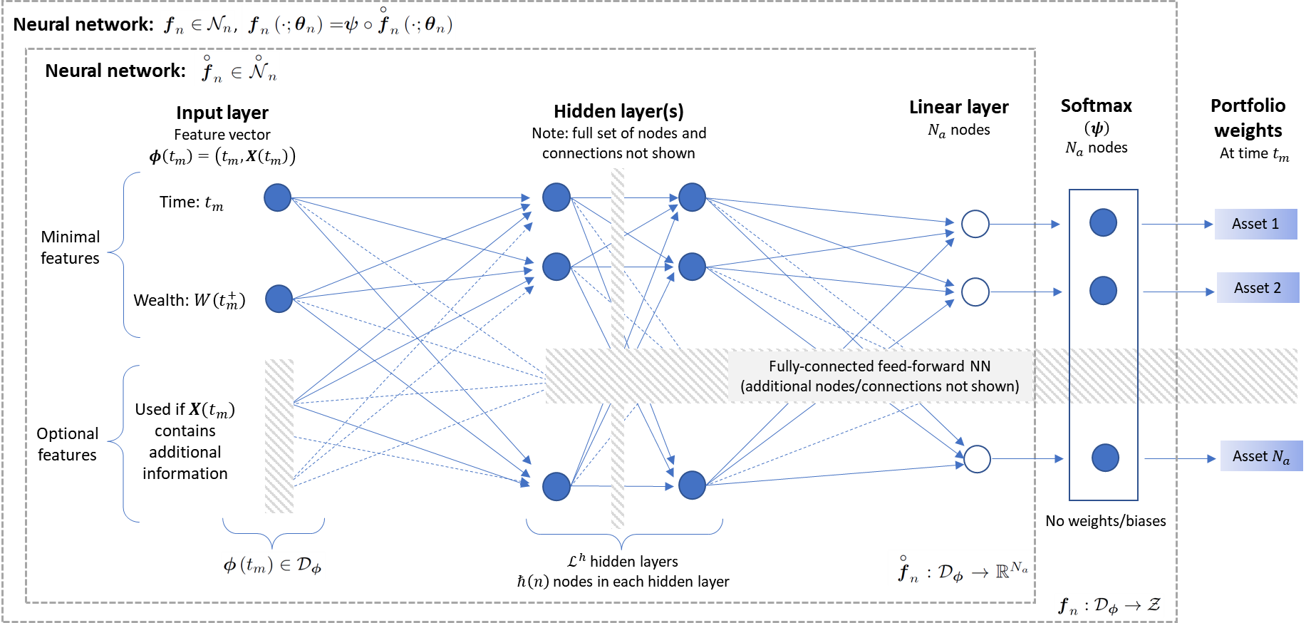
Figure A.1: Illustration of the interpretation of the NN $\boldsymbol{f}_{n}\left(\cdot;\boldsymbol{\theta}_{n}\right)$ as a composition of the softmax $\boldsymbol{\psi}$ and the NN $\overset{\circ}{\boldsymbol{f}}_{n}\left(\cdot;\boldsymbol{\theta}_{n}\right)$ as per equation (A.15).

If Assumption 3.2 and Assumption A.3 are applicable, the wealth dynamics (3.7) using the optimal control is given by

$$W^{\ast}\left(t_{m+1}^{-};\boldsymbol{p}^{\ast},\boldsymbol{Y}\right) = W^{\ast}\left(t_{m}^{+};\boldsymbol{p}^{\ast},\boldsymbol{Y}\right)\cdot\sum_{i=1}^{N_{a}}p_{i}^{\ast}\left(t_{m},W^{\ast}\left(t_{m}^{+};\boldsymbol{p}^{\ast},\boldsymbol{Y}\right)\right)\cdot Y_{i}\left(t_{m}\right),\qquad t_{m}\in\mathcal{T},$$ (A.20)

where we recall that $W^{\ast}\left(t_{m}^{+};\boldsymbol{p}^{\ast},\boldsymbol{Y}\right)=W^{\ast}\left(t_{m}^{-};\boldsymbol{p}^{\ast},\boldsymbol{Y}\right)+q\left(t_{m}\right)$, $\boldsymbol{X}^{\ast}\left(t_{m}\right)=W^{\ast}\left(t_{m}^{+};\boldsymbol{p}^{\ast},\boldsymbol{Y}\right)$ and $W^{\ast}\left(t_{N_{rb}}^{-}\right)\coloneqq W^{\ast}\left(T\right)$. Furthermore, associated with every NN in the sequence $\boldsymbol{f}_{n}^{\ast}\left(\cdot,\boldsymbol{\theta}_{n}^{\ast}\right)\in\mathcal{N}_{n}$ identified in Lemma A.5, we have the corresponding wealth dynamics as per (3.14) that satisfies

$$W^{\ast}\left(t_{m+1}^{-};\boldsymbol{\theta}_{n}^{\ast},\boldsymbol{Y}\right) =W^{\ast}\left(t_{m}^{+};\boldsymbol{\theta}_{n}^{\ast},\boldsymbol{Y}\right)\cdot\sum_{i=1}^{N_{a}}f_{n,i}^{\ast}\left(t_{m},W^{\ast}\left(t_{m}^{+};\boldsymbol{\theta}_{n}^{\ast},\boldsymbol{Y}\right);\boldsymbol{\theta}_{n}^{\ast}\right)\cdot Y_{i}\left(t_{m}\right),\qquad t_{m}\in\mathcal{T},n\in\mathbb{N}.$$ (A.21)

The following lemma justifies the use of the notation $W^{\ast}$ in the wealth dynamics (A.21).

Lemma A.6.

(Convergence to optimal wealth) Suppose that Assumption A.2 and Assumption A.3 hold. Let $\boldsymbol{f}_{n}^{\ast}\left(\cdot,\boldsymbol{\theta}_{n}^{\ast}\right)\in\mathcal{N}_{n}$ be the sequence identified in Lemma A.5 such that (A.10) holds. Then the wealth dynamics $W^{\ast}\left(t;\boldsymbol{\theta}_{n}^{\ast},\boldsymbol{Y}\right)$ associated with each $\boldsymbol{f}_{n}^{\ast}$, obtained as per (A.21), converges to the true optimal wealth dynamics $W^{\ast}\left(t;\boldsymbol{p}^{\ast},\boldsymbol{Y}\right)$ as $n\rightarrow\infty$ almost surely. In more detail, we have

$$\lim_{n\rightarrow\infty}W^{\ast}\left(t_{m}^{-};\boldsymbol{\theta}_{n}^{\ast},\boldsymbol{Y}\right) = W^{\ast}\left(t_{m}^{-};\boldsymbol{p}^{\ast},\boldsymbol{Y}\right)\quad\textrm{a.s.},\qquad\forall t_{m}\in\mathcal{T},$$ (A.22)

and

$$\lim_{n\rightarrow\infty}W^{\ast}\left(T;\boldsymbol{\theta}_{n}^{\ast},\boldsymbol{Y}\right) = W^{\ast}\left(T;\boldsymbol{p}^{\ast},\boldsymbol{Y}\right)\quad\textrm{a.s.}$$ (A.23)

Proof.

Note that (A.23) is stated separately since the terminal time $T$ is not a rebalancing time (see (2.1)) and the terminal wealth is critical in the evaluation of the objective functional.

At the start of the time horizon $\left[t_{0},T\right]$, we are given the initial wealth $W\left(t_{0}^{-}\right)=w_{0}>0$. Therefore, at the first rebalancing time $t_{0}\in\mathcal{T}$, the wealth available for investment does not depend on the control, so that

$$w_{0}^{+}\coloneqq w_{0}+q\left(t_{0}\right)=W^{\ast}\left(t_{0}^{+};\boldsymbol{\theta}_{n}^{\ast},\boldsymbol{Y}\right)=W^{\ast}\left(t_{0}^{+};\boldsymbol{p}^{\ast},\boldsymbol{Y}\right),\qquad\forall n\in\mathbb{N}.$$ (A.24)

Using dynamics (A.20) and (A.21) to compare the wealth at time $t_{0}+\Delta t=t_{1}\in\mathcal{T}$, we have

$$\lim_{n\rightarrow\infty}W^{\ast}\left(t_{1}^{-};\boldsymbol{\theta}_{n}^{\ast},\boldsymbol{Y}\right)-W^{\ast}\left(t_{1}^{-};\boldsymbol{p}^{\ast},\boldsymbol{Y}\right) = w_{0}^{+}\cdot\sum_{i=1}^{N_{a}}\left[\lim_{n\rightarrow\infty}f_{n,i}^{\ast}\left(t_{0},w_{0}^{+};\boldsymbol{\theta}_{n}^{\ast}\right)-p_{i}^{\ast}\left(t_{0},w_{0}^{+}\right)\right]\cdot Y_{i}\left(t_{0}\right)$$ (A.25)

$$= 0\qquad\textrm{a.s.},$$

which follows from Lemma A.5 and the fact that $Y_{i}\left(t_{0}\right)<\infty$ a.s. by assumption (see definition (2.6)).

For purposes of induction, assume that at some $t_{m}\in\mathcal{T}$, we have

$$\lim_{n\rightarrow\infty}W^{\ast}\left(t_{m}^{-};\boldsymbol{\theta}_{n}^{\ast},\boldsymbol{Y}\right) = W^{\ast}\left(t_{m}^{-};\boldsymbol{p}^{\ast},\boldsymbol{Y}\right)\qquad\textrm{a.s.}$$ (A.26)

If (A.26) holds, then we have

$$\lim_{n\rightarrow\infty}W^{\ast}\left(t_{m}^{+};\boldsymbol{\theta}_{n}^{\ast},\boldsymbol{Y}\right)=\lim_{n\rightarrow\infty}\left[W^{\ast}\left(t_{m}^{-};\boldsymbol{\theta}_{n}^{\ast},\boldsymbol{Y}\right)+q\left(t_{m}\right)\right]=W^{\ast}\left(t_{m}^{+};\boldsymbol{p}^{\ast},\boldsymbol{Y}\right)\qquad\textrm{a.s.},$$ (A.27)

as well as

$$\lim_{n\rightarrow\infty}\left|f_{n,i}^{\ast}\left(t_{m},W^{\ast}\left(t_{m}^{+};\boldsymbol{\theta}_{n}^{\ast},\boldsymbol{Y}\right);\boldsymbol{\theta}_{n}^{\ast}\right)-p_{i}^{\ast}\left(t_{m},W^{\ast}\left(t_{m}^{+};\boldsymbol{p}^{\ast},\boldsymbol{Y}\right)\right)\right|$$ (A.28)

$$\leq \lim_{n\rightarrow\infty}\left|f_{n,i}^{\ast}\left(t_{m},W^{\ast}\left(t_{m}^{+};\boldsymbol{\theta}_{n}^{\ast},\boldsymbol{Y}\right);\boldsymbol{\theta}_{n}^{\ast}\right)-p_{i}^{\ast}\left(t_{m},W^{\ast}\left(t_{m}^{+};\boldsymbol{\theta}_{n}^{\ast},\boldsymbol{Y}\right)\right)\right|$$

$$+\lim_{n\rightarrow\infty}\left|p_{i}^{\ast}\left(t_{m},W^{\ast}\left(t_{m}^{+};\boldsymbol{\theta}_{n}^{\ast},\boldsymbol{Y}\right)\right)-p_{i}^{\ast}\left(t_{m},W^{\ast}\left(t_{m}^{+};\boldsymbol{p}^{\ast},\boldsymbol{Y}\right)\right)\right|$$

$$\leq \lim_{n\rightarrow\infty}\sup_{\boldsymbol{\phi}\in\mathcal{D}_{\boldsymbol{\phi}}}\left|f_{n,i}^{\ast}\left(\boldsymbol{\phi};\boldsymbol{\theta}_{n}^{\ast}\right)-p_{i}^{\ast}\left(\boldsymbol{\phi}\right)\right|$$

$$= 0\qquad\textrm{a.s.},\qquad\forall i=1,...,N_{a},$$

which is a consequence of Lemma A.5 and the continuity of $\boldsymbol{p}^{\ast}\in C\left(\mathcal{D}_{\boldsymbol{\phi}},\mathcal{Z}\right)$. From (A.27) and (A.28), we therefore conclude that

$$\lim_{n\rightarrow\infty}\left|W^{\ast}\left(t_{m}^{+};\boldsymbol{\theta}_{n}^{\ast},\boldsymbol{Y}\right)\cdot f_{n,i}^{\ast}\left(t_{m},W^{\ast}\left(t_{m}^{+};\boldsymbol{\theta}_{n}^{\ast},\boldsymbol{Y}\right);\boldsymbol{\theta}_{n}^{\ast}\right)-W^{\ast}\left(t_{m}^{+};\boldsymbol{p}^{\ast},\boldsymbol{Y}\right)\cdot p_{i}^{\ast}\left(t_{m},W^{\ast}\left(t_{m}^{+};\boldsymbol{p}^{\ast},\boldsymbol{Y}\right)\right)\right|$$

$$= 0\qquad\textrm{a.s.},\qquad\forall i=1,...,N_{a}.$$ (A.29)

Using dynamics (A.20) and (A.21) to compare the wealth at time $t_{m}+\Delta t=t_{m+1}$, we have

$$\lim_{n\rightarrow\infty}W^{\ast}\left(t_{m+1}^{-};\boldsymbol{\theta}_{n}^{\ast},\boldsymbol{Y}\right)-W^{\ast}\left(t_{m+1}^{-};\boldsymbol{p}^{\ast},\boldsymbol{Y}\right) = \lim_{n\rightarrow\infty}W^{\ast}\left(t_{m}^{+};\boldsymbol{\theta}_{n}^{\ast},\boldsymbol{Y}\right)\cdot\sum_{i=1}^{N_{a}}f_{n,i}^{\ast}\left(t_{m},W^{\ast}\left(t_{m}^{+};\boldsymbol{\theta}_{n}^{\ast},\boldsymbol{Y}\right);\boldsymbol{\theta}_{n}^{\ast}\right)\cdot Y_{i}\left(t_{m}\right)$$ (A.30)

$$-W^{\ast}\left(t_{m}^{+};\boldsymbol{p}^{\ast},\boldsymbol{Y}\right)\cdot\sum_{i=1}^{N_{a}}p_{i}^{\ast}\left(t_{m},W^{\ast}\left(t_{m}^{+};\boldsymbol{p}^{\ast},\boldsymbol{Y}\right)\right)\cdot Y_{i}\left(t_{m}\right)$$

$$= 0\qquad\textrm{a.s.},$$

which follows from (A.29) and $Y_{i}\left(t_{m}\right)<\infty$ a.s. By induction, we therefore conclude that (A.22) holds if $t_{m+1}\in\mathcal{T}$ (i.e. if $m<N_{rb}-1$), and (A.23) holds in the case where $t_{m+1}=t_{N_{rb}}=T$ (i.e. $m=N_{rb}-1$). ∎

The following lemma establishes the convergence of the sequence of objective functionals using the NN approximations identified in Lemma A.5.

Lemma A.7.

(Convergence of objective functionals) Suppose that Assumption A.2 and Assumption A.3 hold. Let $\boldsymbol{f}_{n}^{\ast}\left(\cdot,\boldsymbol{\theta}_{n}^{\ast}\right)\in\mathcal{N}_{n}$ be the sequence identified in Lemma A.5 such that (A.10) holds. Then

$$\lim_{n\rightarrow\infty}J_{n}\left(\boldsymbol{\theta}_{n}^{\ast},\xi;t_{0},w_{0}\right) = J\left(\boldsymbol{p}^{\ast},\xi;t_{0},w_{0}\right),\qquad\forall\xi\in\mathbb{R},$$ (A.31)

where $J_{n}$ is defined in (3.13), and $J$ is defined in (3.6).

Proof.

Let $\xi\in\mathbb{R}$ be arbitrary. By Lemma A.6 and the continuity of $F$, we have

$$\lim_{n\rightarrow\infty}F\left(W^{\ast}\left(T;\boldsymbol{\theta}_{n}^{\ast},\boldsymbol{Y}\right),\xi\right) = F\left(W^{\ast}\left(T;\boldsymbol{p}^{\ast},\boldsymbol{Y}\right),\xi\right)\qquad\textrm{a.s}.$$ (A.32)

Therefore, by using the boundedness of wealth as per Assumption A.3, the dominated convergence theorem gives

$$\lim_{n\rightarrow\infty}E^{t_{0},w_{0}}\left[F\left(W^{\ast}\left(T;\boldsymbol{\theta}_{n}^{\ast},\boldsymbol{Y}\right),\xi\right)\right] = E^{t_{0},w_{0}}\left[F\left(W^{\ast}\left(T;\boldsymbol{p}^{\ast},\boldsymbol{Y}\right),\xi\right)\right].$$ (A.33)

Similarly, by the continuity of $G$, Lemma A.6, the boundedness of wealth and the dominated convergence theorem, we have

$$\lim_{n\rightarrow\infty}E^{t_{0},w_{0}}\left[G\left(W^{\ast}\left(T;\boldsymbol{\theta}_{n}^{\ast},\boldsymbol{Y}\right),E^{t_{0},w_{0}}\left[W^{\ast}\left(T;\boldsymbol{\theta}_{n}^{\ast},\boldsymbol{Y}\right)\right],w_{0},\xi\right)\right]$$ (A.34)

$$= E^{t_{0},w_{0}}\left[G\left(W^{\ast}\left(T;\boldsymbol{p}^{\ast},\boldsymbol{Y}\right),E^{t_{0},w_{0}}\left[W^{\ast}\left(T;\boldsymbol{p}^{\ast},\boldsymbol{Y}\right)\right],w_{0},\xi\right)\right].$$

Finally, using the definitions of $J$ in (3.6) and $J_{n}$ in (3.13), we combine (A.33) and (A.34) to conclude (A.31). ∎

Proof of Theorem 4.1

Using the preceding results, we are finally in the position to prove Theorem 4.1. Note that this proof also motivates the use of the notation $\boldsymbol{f}_{n}^{\ast}\left(\cdot,\boldsymbol{\theta}_{n}^{\ast}\right)$ and its associated wealth $W^{\ast}\left(T;\boldsymbol{\theta}_{n}^{\ast},\boldsymbol{Y}\right)$ for the sequence of NNs identified in Lemma A.5 and subsequently used in Lemmas A.6 and A.7 above.

Since $\xi\rightarrow F\left(w,\xi\right)$ and $\xi\rightarrow G\left(w,x,w_{0},\xi\right)$ are convex by Assumption A.2, and the convexity is preserved by taking the expectation of $F$, we have the result that $\xi\rightarrow J_{n}\left(\boldsymbol{\theta}_{n},\xi;t_{0},w_{0}\right)$ and $\xi\rightarrow J\left(\boldsymbol{p},\xi;t_{0},w_{0}\right)$ are also convex, so that the infimum over $\xi\in\mathbb{R}$ in each case can be attained and is unique. With $\boldsymbol{p}^{\ast}$ still denoting the optimal control, define $\xi^{\ast}$ as the value

$$\xi^{\ast} \coloneqq \inf_{\xi\in\mathbb{R}}J\left(\boldsymbol{p}^{\ast},\xi;t_{0},w_{0}\right).$$ (A.35)

Since $\mathcal{N}_{n}\subset C\left(\mathcal{D}_{\boldsymbol{\phi}},\mathcal{Z}\right)$, we have, for all $\xi\in\mathbb{R}$ and all $n\in\mathbb{N}$,

$$\inf_{\boldsymbol{\theta}_{n}\in\mathbb{R}^{\nu_{n}}}J_{n}\left(\boldsymbol{\theta}_{n},\xi;t_{0},w_{0}\right)=\inf_{\boldsymbol{f}_{n}\left(\cdot;\boldsymbol{\theta}_{n}\right)\in\mathcal{N}_{n}}J\left(\boldsymbol{f}_{n},\xi;t_{0},w_{0}\right) \geq \inf_{\boldsymbol{p}\in C\left(\mathcal{D}_{\boldsymbol{\phi}},\mathcal{Z}\right)}J\left(\boldsymbol{p},\xi;t_{0},w_{0}\right).$$ (A.36)

Taking the infimum in (A.36) over $\xi\in\mathbb{R}$, and exchanging the order of minimization, we therefore have

$$\inf_{\left(\boldsymbol{\theta}_{n},\xi\right)\in\mathbb{R}^{\nu_{n}+1}}J_{n}\left(\boldsymbol{\theta}_{n},\xi;t_{0},w_{0}\right) = \inf_{\boldsymbol{\theta}_{n}\in\mathbb{R}^{\nu_{n}}}\inf_{\xi\in\mathbb{R}}J_{n}\left(\boldsymbol{\theta}_{n},\xi;t_{0},w_{0}\right)$$ (A.37)

$$\geq \inf_{\boldsymbol{p}\in C\left(\mathcal{D}_{\boldsymbol{\phi}},\mathcal{Z}\right)}\inf_{\xi\in\mathbb{R}}J\left(\boldsymbol{p},\xi;t_{0},w_{0}\right),\qquad\forall n\in\mathbb{N}.$$

Taking limits in (A.37), we obtain

$$\lim_{n\rightarrow\infty}\inf_{\left(\boldsymbol{\theta}_{n},\xi\right)\in\mathbb{R}^{\nu_{n}+1}}J_{n}\left(\boldsymbol{\theta}_{n},\xi;t_{0},w_{0}\right) \geq \inf_{\xi\in\mathbb{R}}\inf_{\boldsymbol{p}\in C\left(\mathcal{D}_{\boldsymbol{\phi}},\mathcal{Z}\right)}J\left(\boldsymbol{p},\xi;t_{0},w_{0}\right).$$ (A.38)

Now consider specifically the sequence $\boldsymbol{f}_{n}^{\ast}\left(\cdot,\boldsymbol{\theta}_{n}^{\ast}\right)$ identified in Lemma A.5 and the value $\xi^{\ast}$ in (A.35). Since $\boldsymbol{f}_{n}^{\ast}\left(\cdot,\boldsymbol{\theta}_{n}^{\ast}\right)\in\mathcal{N}_{n}$ (so that $\boldsymbol{\theta}_{n}^{\ast}\in\mathbb{R}^{\nu_{n}}$) and $\xi^{\ast}\in\mathbb{R}$, we have

$$\inf_{\left(\boldsymbol{\theta}_{n},\xi\right)\in\mathbb{R}^{\nu_{n}+1}}J_{n}\left(\boldsymbol{\theta}_{n},\xi;t_{0},w_{0}\right) \leq J_{n}\left(\boldsymbol{\theta}_{n}^{\ast},\xi^{\ast};t_{0},w_{0}\right),\qquad\forall n\in\mathbb{N}.$$ (A.39)

By Lemma A.7, we have

$$\lim_{n\rightarrow\infty}J_{n}\left(\boldsymbol{\theta}_{n}^{\ast},\xi^{\ast};t_{0},w_{0}\right) = J\left(\boldsymbol{p}^{\ast},\xi^{\ast};t_{0},w_{0}\right),\quad\textrm{ where }\xi^{\ast}\textrm{ is given by \eqref{eq: Appendix xi star}}.$$ (A.40)

Therefore, taking limits in (A.39) and using (A.40), we obtain the inequality

$$\lim_{n\rightarrow\infty}\inf_{\left(\boldsymbol{\theta}_{n},\xi\right)\in\mathbb{R}^{\nu_{n}+1}}J_{n}\left(\boldsymbol{\theta}_{n},\xi;t_{0},w_{0}\right) \leq \lim_{n\rightarrow\infty}J_{n}\left(\boldsymbol{\theta}_{n}^{\ast},\xi^{\ast};t_{0},w_{0}\right)$$ (A.41)

$$= J\left(\boldsymbol{p}^{\ast},\xi^{\ast};t_{0},w_{0}\right)$$

$$= \inf_{\xi\in\mathbb{R}}\inf_{\boldsymbol{p}\in C\left(\mathcal{D}_{\boldsymbol{\phi}},\mathcal{Z}\right)}J\left(\boldsymbol{p},\xi;t_{0},w_{0}\right).$$

Combining (A.38) and (A.41), we therefore have equality in both (A.38) and (A.41), and obtain

$$\lim_{n\rightarrow\infty}\inf_{\left(\boldsymbol{\theta}_{n},\xi\right)\in\mathbb{R}^{\nu_{n}+1}}J_{n}\left(\boldsymbol{\theta}_{n},\xi;t_{0},w_{0}\right) = \inf_{\xi\in\mathbb{R}}\inf_{\boldsymbol{p}\in C\left(\mathcal{D}_{\boldsymbol{\phi}},\mathcal{Z}\right)}J\left(\boldsymbol{p},\xi;t_{0},w_{0}\right),$$ (A.42)

which concludes the proof of Theorem 4.1. Finally, the notation $\boldsymbol{f}_{n}^{\ast}\left(\cdot,\boldsymbol{\theta}_{n}^{\ast}\right)$ in Lemma A.5 is motivated by the fact that equality holds in (A.41).∎

A.4 Proof of Theorem 4.2

We start with the following auxiliary result, which is essentially a version of the law of large numbers applicable to the current setting.

Lemma A.8.

(Applicable version of the law of large numbers) Suppose that Assumption A.2, Assumption A.3 and Assumption A.4 hold. Then

$$\sup_{\boldsymbol{\theta}_{n}\in\mathbb{R}^{\nu_{n}}}\left|\frac{1}{n}\sum_{j=1}^{n}W^{\left(j\right)}\left(T;\boldsymbol{\theta}_{n},\mathcal{Y}_{n}\right)-E^{t_{0},w_{0}}\left[W\left(T;\boldsymbol{\theta}_{n},\boldsymbol{Y}\right)\right]\right| \overset{P}{\longrightarrow} 0,\;\textrm{as }n\rightarrow\infty,$$ (A.43)

and

$$\sup_{\left(\boldsymbol{\theta}_{n},\xi\right)\in\mathbb{R}^{\nu_{n}+1}}\left|\frac{1}{n}\sum_{j=1}^{n}F\left(W^{\left(j\right)}\left(T;\boldsymbol{\theta}_{n},\mathcal{Y}_{n}\right),\xi\right)-E^{t_{0},w_{0}}\left[F\left(W\left(T;\boldsymbol{\theta}_{n},\boldsymbol{Y}\right),\xi\right)\right]\right| \overset{P}{\longrightarrow} 0,\;\textrm{as }n\rightarrow\infty.$$ (A.44)

Proof.

Since for any fixed number of hidden layers, our NN formulation also requires $\mathcal{O}\left(\hbar_{n}\right)$ evaluations of the exponential function, exactly the same steps as in Tsang and Wong (2020) (specifically, see Corollary 7.4 and Theorem 4.3 in Tsang and Wong (2020)) can be used to establish (A.43) and (A.44). ∎

The following lemma establishes a required auxiliary result involving the function $G$.

Lemma A.9.

(Convergence of $G$ in probability) Suppose that Assumption A.2, Assumption A.3 and Assumption A.4 hold. Then

$$\sup_{\left(\boldsymbol{\theta}_{n},\xi\right)\in\mathbb{R}^{\nu_{n}+1}}\left|\frac{1}{n}\sum_{j=1}^{n}G\left(W^{\left(j\right)}\left(T;\boldsymbol{\theta}_{n},\mathcal{Y}_{n}\right),\frac{1}{n}\sum_{k=1}^{n}W^{\left(k\right)}\left(T;\boldsymbol{\theta}_{n},\mathcal{Y}_{n}\right),w_{0},\xi\right)\right.$$

$$\left.-E^{t_{0},w_{0}}\left[G\left(W\left(T;\boldsymbol{\theta}_{n},\boldsymbol{Y}\right),E^{t_{0},w_{0}}\left[W\left(T;\boldsymbol{\theta}_{n},\boldsymbol{Y}\right)\right],w_{0},\xi\right)\right]\begin{array}[]{c}\!\!\!\!\!\!\!\!\\ \!\!\!\!\!\!\!\!\end{array}\right| \overset{P}{\longrightarrow} 0,$$ (A.47)

as $n\rightarrow\infty$.

Proof.

For given values of $\xi\in\mathbb{R}$, $w_{0}>0$ and $w\in\mathbb{R}$, consider the function $x\rightarrow G\left(x,w,w_{0},\xi\right)$. By the results of Lemma A.8, we have

$$\sup_{\left(\boldsymbol{\theta}_{n},\xi\right)\in\mathbb{R}^{\nu_{n}+1}}\left|\frac{1}{n}\sum_{j=1}^{n}G\left(W^{\left(j\right)}\left(T;\boldsymbol{\theta}_{n},\mathcal{Y}_{n}\right),w,w_{0},\xi\right)-E^{t_{0},w_{0}}\left[G\left(W\left(T;\boldsymbol{\theta}_{n},\boldsymbol{Y}\right),w,w_{0},\xi\right)\right]\right| \overset{P}{\longrightarrow} 0,$$ (A.48)

as $n\rightarrow\infty$. Keeping $x$ fixed, consider the function $w\rightarrow G\left(x,w,w_{0},\xi\right):\left[0,w_{max}\right]\rightarrow\mathbb{R}$. Since $G$ is continuous, there exists a sequence of functions $\left(G_{m}\right)_{m\in\mathbb{N}}$, where for each $m\in\mathbb{N}$, the function $w\rightarrow G_{m}\left(x,w,w_{0},\xi\right):\left[0,w_{max}\right]\rightarrow\mathbb{R}$ is $L_{m}$-Lipschitz, such that $\left(G_{m}\right)$ converges uniformly to $G$ on $\left[0,w_{max}\right]$ - see for example Miculescu (2000). Therefore, for an arbitrary value of $\epsilon>0$, there exists a sufficiently large value $\tilde{m}\in\mathbb{N}$ such that

$$\left|G_{\tilde{m}}\left(x,w,w_{0},\xi\right)-G\left(x,w,w_{0},\xi\right)\right|< \frac{\epsilon}{2},\qquad\forall w\in\left[0,w_{max}\right].$$ (A.49)

Observing that $\frac{1}{n}\sum_{j=1}^{n}W^{\left(j\right)}\left(T;\boldsymbol{\theta}_{n},\mathcal{Y}_{n}\right)\in\left[0,w_{max}\right]$ and by the monotonicity of expectation we also have $E^{t_{0},w_{0}}\left[W\left(T;\boldsymbol{\theta}_{n},\boldsymbol{Y}\right)\right]\in\left[0,w_{max}\right]$, we use (A.49) to obtain

$$\left|G_{\tilde{m}}\left(x,\frac{1}{n}\sum_{j=1}^{n}W^{\left(j\right)}\left(T;\boldsymbol{\theta}_{n},\mathcal{Y}_{n}\right),w_{0},\xi\right)-G\left(x,\frac{1}{n}\sum_{j=1}^{n}W^{\left(j\right)}\left(T;\boldsymbol{\theta}_{n},\mathcal{Y}_{n}\right),w_{0},\xi\right)\right|$$ (A.52)

$$+\left|G_{\tilde{m}}\left(x,E^{t_{0},w_{0}}\left[W\left(T;\boldsymbol{\theta}_{n},\boldsymbol{Y}\right)\right],w_{0},\xi\right)-G\left(x,E^{t_{0},w_{0}}\left[W\left(T;\boldsymbol{\theta}_{n},\boldsymbol{Y}\right)\right],w_{0},\xi\right)\begin{array}[]{c}\!\!\!\!\!\!\!\!\\ \!\!\!\!\!\!\!\!\end{array}\right|$$

$$< \epsilon,$$ (A.53)

for any given values of $\xi\in\mathbb{R}$ and $w_{0}>0$. In addition, since $G_{\tilde{m}}$ is $L_{\tilde{m}}$-Lipschitz, we have

$$\left|G_{\widetilde{m}}\left(x,\frac{1}{n}\sum_{j=1}^{n}W^{\left(j\right)}\left(T;\boldsymbol{\theta}_{n},\mathcal{Y}_{n}\right),w_{0},\xi\right)-G_{\widetilde{m}}\left(x,E^{t_{0},w_{0}}\left[W\left(T;\boldsymbol{\theta}_{n},\boldsymbol{Y}\right)\right],w_{0},\xi\right)\right|$$ (A.54)

$$\leq L_{\widetilde{m}}\cdot\left|\frac{1}{n}\sum_{j=1}^{n}W^{\left(j\right)}\left(T;\boldsymbol{\theta}_{n},\mathcal{Y}_{n}\right)-E^{t_{0},w_{0}}\left[W\left(T;\boldsymbol{\theta}_{n},\boldsymbol{Y}\right)\right]\right|.$$

Using (A.53) and (A.54) as well as the triangle inequality, we therefore have

$$\left|G\left(x,\frac{1}{n}\sum_{j=1}^{n}W^{\left(j\right)}\left(T;\boldsymbol{\theta}_{n},\mathcal{Y}_{n}\right),w_{0},\xi\right)-G\left(x,E^{t_{0},w_{0}}\left[W\left(T;\boldsymbol{\theta}_{n},\boldsymbol{Y}\right)\right]\right),w_{0},\xi\right|$$ (A.55)

$$< \epsilon+L_{\widetilde{m}}\cdot\left|\frac{1}{n}\sum_{j=1}^{n}W^{\left(j\right)}\left(T;\boldsymbol{\theta}_{n},\mathcal{Y}_{n}\right)-E^{t_{0},w_{0}}\left[W\left(T;\boldsymbol{\theta}_{n},\boldsymbol{Y}\right)\right]\right|,$$

for any given values of $\xi\in\mathbb{R}$ and $w_{0}>0$. Taking the supremum over $\left(\boldsymbol{\theta}_{n},\xi\right)\in\mathbb{R}^{\nu_{n}+1}$ in (A.55), using the result (A.43) from Lemma A.8 as well as the fact that $\epsilon>0$ was arbitrary, we therefore have

$$\sup_{\left(\boldsymbol{\theta}_{n},\xi\right)\in\mathbb{R}^{\nu_{n}+1}}\left|G\left(x,\frac{1}{n}\sum_{k=1}^{n}W^{\left(k\right)}\left(T;\boldsymbol{\theta}_{n},\mathcal{Y}_{n}\right),w_{0},\xi\right)-G\left(x,E^{t_{0},w_{0}}\left[W\left(T;\boldsymbol{\theta}_{n},\boldsymbol{Y}\right)\right],w_{0},\xi\right)\right| \overset{P}{\longrightarrow} 0.$$ (A.56)

The results (A.48) and (A.56), together with the triangle inequality, therefore gives

$$\sup_{\left(\boldsymbol{\theta}_{n},\xi\right)\in\mathbb{R}^{\nu_{n}+1}}\left|\frac{1}{n}\sum_{j=1}^{n}G\left(W^{\left(j\right)}\left(T;\boldsymbol{\theta}_{n},\mathcal{Y}_{n}\right),\frac{1}{n}\sum_{k=1}^{n}W^{\left(k\right)}\left(T;\boldsymbol{\theta}_{n},\mathcal{Y}_{n}\right),w_{0},\xi\right)\right.$$ (A.65)

$$\qquad\qquad\left.\qquad\qquad-E^{t_{0},w_{0}}\left[G\left(W\left(T;\boldsymbol{\theta}_{n},\boldsymbol{Y}\right),E^{t_{0},w_{0}}\left[W\left(T;\boldsymbol{\theta}_{n},\boldsymbol{Y}\right)\right],w_{0},\xi\right)\right]\begin{array}[]{c}\!\!\!\!\!\!\!\!\\ \!\!\!\!\!\!\!\!\end{array}\right|$$

$$\leq \frac{1}{n}\sum_{j=1}^{n}\sup_{\left(\boldsymbol{\theta}_{n},\xi\right)\in\mathbb{R}^{\nu_{n}+1}}\left|\frac{1}{n}\sum_{j=1}^{n}G\left(W^{\left(j\right)}\left(T;\boldsymbol{\theta}_{n},\mathcal{Y}_{n}\right),\frac{1}{n}\sum_{k=1}^{n}W^{\left(k\right)}\left(T;\boldsymbol{\theta}_{n},\mathcal{Y}_{n}\right),w_{0},\xi\right)\right.$$

$$\qquad\qquad\left.\qquad\qquad-G\left(W^{\left(j\right)}\left(T;\boldsymbol{\theta}_{n},\mathcal{Y}_{n}\right),E^{t_{0},w_{0}}\left[W\left(T;\boldsymbol{\theta}_{n},\boldsymbol{Y}\right)\right],w_{0},\xi\right)\begin{array}[]{c}\!\!\!\!\!\!\!\!\\ \!\!\!\!\!\!\!\!\end{array}\right|$$

$$+\sup_{\left(\boldsymbol{\theta}_{n},\xi\right)\in\mathbb{R}^{\nu_{n}+1}}\left|\frac{1}{n}\sum_{j=1}^{n}G\left(W^{\left(j\right)}\left(T;\boldsymbol{\theta}_{n},\mathcal{Y}_{n}\right),E^{t_{0},w_{0}}\left[W\left(T;\boldsymbol{\theta}_{n},\boldsymbol{Y}\right)\right],w_{0},\xi\right)\right.$$

$$\qquad\qquad\left.\qquad\qquad-E^{t_{0},w_{0}}\left[G\left(W\left(T;\boldsymbol{\theta}_{n},\boldsymbol{Y}\right),E^{t_{0},w_{0}}\left[W\left(T;\boldsymbol{\theta}_{n},\boldsymbol{Y}\right)\right],w_{0},\xi\right)\right]\begin{array}[]{c}\!\!\!\!\!\!\!\!\\ \!\!\!\!\!\!\!\!\end{array}\right|$$

$$\overset{P}{\longrightarrow} 0\qquad\textrm{as }n\rightarrow\infty.$$ (A.66)

∎

Proof of Theorem 4.2

The expression in (4.2), together with the triangle inequality, imply that

$$\left|\inf_{\left(\boldsymbol{\theta}_{n},\xi\right)\in\mathbb{R}^{\nu_{n}+1}}\hat{J}_{n}\left(\boldsymbol{\theta}_{n},\xi;t_{0},w_{0},\mathcal{Y}_{n}\right)-\inf_{\xi\in\mathbb{R}}\inf_{\boldsymbol{p}\in C\left(\mathcal{D}_{\boldsymbol{\phi}},\mathcal{Z}\right)}J\left(\boldsymbol{p},\xi;t_{0},w_{0}\right)\right|$$ (A.68)

$$\leq \left|\inf_{\left(\boldsymbol{\theta}_{n},\xi\right)\in\mathbb{R}^{\nu_{n}+1}}\hat{J}_{n}\left(\boldsymbol{\theta}_{n},\xi;t_{0},w_{0},\mathcal{Y}_{n}\right)-\inf_{\left(\boldsymbol{\theta}_{n},\xi\right)\in\mathbb{R}^{\eta_{n}+1}}J_{n}\left(\boldsymbol{\theta}_{n},\xi;t_{0},w_{0}\right)\right|$$

$$+\left|\inf_{\left(\boldsymbol{\theta}_{n},\xi\right)\in\mathbb{R}^{\nu_{n}+1}}J_{n}\left(\boldsymbol{\theta}_{n},\xi;t_{0},w_{0}\right)-\inf_{\xi\in\mathbb{R}}\inf_{\boldsymbol{p}\in C\left(\mathcal{D}_{\boldsymbol{\phi}},\mathcal{Z}\right)}J\left(\boldsymbol{p},\xi;t_{0},w_{0}\right)\right|.$$

Using the definitions of $\hat{J}_{n}\left(\boldsymbol{\theta}_{n},\xi;t_{0},w_{0},\mathcal{Y}_{n}\right)$ in (3.19) and $J_{n}\left(\boldsymbol{\theta}_{n},\xi;t_{0},w_{0}\right)$ in (3.13), the expression (A.68) gives

$$\left|\inf_{\left(\boldsymbol{\theta}_{n},\xi\right)\in\mathbb{R}^{\nu_{n}+1}}\hat{J}_{n}\left(\boldsymbol{\theta}_{n},\xi;t_{0},w_{0},\mathcal{Y}_{n}\right)-\inf_{\left(\boldsymbol{\theta}_{n},\xi\right)\in\mathbb{R}^{\eta_{n}+1}}J_{n}\left(\boldsymbol{\theta}_{n},\xi;t_{0},w_{0}\right)\right|$$ (A.71)

$$\leq \sup_{\left(\boldsymbol{\theta}_{n},\xi\right)\in\mathbb{R}^{\nu_{n}+1}}\left|\hat{J}_{n}\left(\boldsymbol{\theta}_{n},\xi;t_{0},w_{0},\mathcal{Y}_{n}\right)-J_{n}\left(\boldsymbol{\theta}_{n},\xi;t_{0},w_{0}\right)\begin{array}[]{c}\!\!\!\!\!\!\!\!\\ \!\!\!\!\!\!\!\!\end{array}\right|$$

$$\leq \sup_{\left(\boldsymbol{\theta}_{n},\xi\right)\in\mathbb{R}^{\nu_{n}+1}}\left|\frac{1}{n}\sum_{j=1}^{n}F\left(W^{\left(j\right)}\left(T;\boldsymbol{\theta}_{n},\mathcal{Y}_{n}\right),\xi\right)-E^{t_{0},w_{0}}\left[F\left(W\left(T;\boldsymbol{\theta}_{n},\boldsymbol{Y}\right),\xi\right)\right]\right|$$ (A.75)

$$+\sup_{\left(\boldsymbol{\theta}_{n},\xi\right)\in\mathbb{R}^{\nu_{n}+1}}\left|\frac{1}{n}\sum_{j=1}^{n}G\left(W^{\left(j\right)}\left(T;\boldsymbol{\theta}_{n},\mathcal{Y}_{n}\right),\frac{1}{n}\sum_{k=1}^{n}W^{\left(k\right)}\left(T;\boldsymbol{\theta}_{n},\mathcal{Y}_{n}\right),w_{0},\xi\right)\right.$$

$$\qquad\qquad\left.\qquad\qquad-E^{t_{0},w_{0}}\left[G\left(W\left(T;\boldsymbol{\theta}_{n},\boldsymbol{Y}\right),E^{t_{0},w_{0}}\left[W\left(T;\boldsymbol{\theta}_{n},\boldsymbol{Y}\right)\right],w_{0},\xi\right)\right]\begin{array}[]{c}\!\!\!\!\!\!\!\!\\ \!\!\!\!\!\!\!\!\end{array}\right|.$$

As per Lemma A.8 and Lemma A.9, (A.75) and (A.75) converge to zero in probability as $n\rightarrow\infty$. As a result, since (A.68) therefore converges to zero in probability as $n\rightarrow\infty$ and, by Theorem 4.1, (A.68) converges to zero as $n\rightarrow\infty$, we conclude that the result (4.2) of Theorem 4.2 holds. ∎

Appendix B NN approach: Selected practical considerations

We summarize some practical considerations with respect to the NN approach:

1. Constructing training and testing datasets $\mathcal{Y}_{n}$ and $\mathcal{Y}_{\hat{n}}^{test}$: Since these sets correspond to finite samples of $\boldsymbol{Y}$ and $\boldsymbol{Y}^{test}$, any data generation technique generating paths of underlying asset returns can be used for the construction of training and testing data sets. As illustrated in Section 5, data generation techniques like (i) Monte Carlo simulation of parametric asset dynamics, (ii) block bootstrap resampling of empirical returns, or for example (iii) GAN-generated synthetic returns can all be employed without difficulty, but we emphasize that the approach remains agnostic regarding the underlying data generation methodology. Note that the underlying data generation assumptions typically differ for $\mathcal{Y}_{n}$ and $\mathcal{Y}_{\hat{n}}^{test}$, respectively, depending on for example the time periods of empirical data considered for in-sample and out-of-sample testing.

   As for the number of paths $n$ in each of $\mathcal{Y}_{n}$ and $\mathcal{Y}_{\hat{n}}^{test}$, experiments show that in the case of measures of tail risk in the objectives such as CVaR (see (2.17)), a significantly larger number of paths are required in order to obtain a sufficiently large sample of tail outcomes in the training and testing data, than for example in cases where variance is the risk measure. To give a concrete examples, at least 2 million paths in the training set of the NN in Subsection 5.2 is required to produce reliable results for the CVaR, whereas 1 million paths in the training set of the NN in Subsection 5.1 are more than sufficient to obtain reliable results.

2. Depth (number of hidden layers $\mathcal{L}^{h}$) and width (number of nodes in each hidden layer $\hbar\left(n\right)$) of the NN: As the examples in Section 5 show, remarkably accurate can be obtained with NNs no deeper than 2 hidden layers and a relatively small number of nodes in each hidden layer. For objectives involving more complex investment strategies such as MCV and Mean - Semi-variance (where, even in the case of two assets, the behavior of the optimal strategy is clearly more complex than in the case of for example the MV-optimal strategy), experiments show that two hidden layers lead to stable and reliable results, with the number of hidden nodes in each hidden layer chosen to be slightly more than the number of assets, for example $\hbar\left(n\right)=N_{a}+2$. For objectives such as DSQ and MV, a single hidden layer is often sufficient.

3. Activation functions: As highlighted in Assumption A.1, we use logistic sigmoid activations as a concrete example for convergence analysis purposes, but that these theoretical results can be modified for any of the commonly-used activations (see for example Sonoda and Murata (2017)). Note that since NNs of one or two hidden layers were found to be very effective in solving the problems under consideration, we did not encounter any problems related to vanishing or exploding gradients in the case of logistic sigmoid activations. However, if deeper NNs are required, activation functions could be changed to e.g. ReLU or ELU without affecting the theoretical foundations for the proposed approach.

4. For the solution of (3.20) by gradient descent, we used the Gadam algorithm of Granziol et al. (2020). This is simply a combination of the Adam algorithm (Kingma and Ba (2015)) with tail iterate averaging for improved convergence properties and variance reduction (Polyak and Juditsky (1992); Mucke et al. (2019); Neu and Rosasco (2018)). For the Adam algorithm component, the default algorithm parameters of Kingma and Ba (2015) performed well in our setting, typically with no more than 50,000 SGD steps. Note that the mini-batch size selected depends on the problem to be solved: we found that mini-batch sizes of at least 1,000 paths of the training data set $\mathcal{Y}_{n}$ are required for measures of tail risk in the objective (such as CVaR), since smaller batch sizes typically means that the tail of the returns distribution is not sufficiently well represented in choosing the descent direction, leading to unreliable results in ground truth analyses.

   While the technical results of Section 5 formally do not require continuous differentiability (in addition to continuity) of the functions $F$ and $G$, improved convergence properties of the SGD algorithm can be obtained if the objective is at least continuously differentiable (see for example Shapiro and Wardi (1996)). For implementation purposes, we can therefore smooth objectives like (2.17) in a straightforward way, by for example replacing $\max\left(x,0\right)$ in (2.17) with a continuously differentiable approximation used in Alexander et al. (2006),

   $$\max\left(x,0\right) \simeq \begin{cases}x,&\textrm{if }x>\lambda_{mcv},\\ \frac{1}{4\lambda_{mcv}}x^{2}+\frac{1}{2}x+\frac{1}{4}\lambda_{mcv},&\textrm{if }-\lambda_{mcv}\leq x\leq\lambda_{mcv}\\ 0,&\textrm{otherwise},\end{cases},$$ (B.1)

   where $\lambda_{mcv}$ is some small smoothing parameter (e.g. $\lambda_{mcv}=10^{-3})$.

   In addition to considering the smoothing of certain objectives, minor modifications to objective functions to avoid (mathematical) ill-posedness may be desirable in certain situations. For example, in the case of the OSQ objective (2.13), the term $\epsilon W(\cdot)$ is added to ensure the problem remains well-posed even if $W(t)\gg\gamma$. In this case, when implementing the numerical solution, small values of $\epsilon$ (for example $\epsilon=10^{-6}$ was chosen in the numerical results of Section 5) do not have a noticeable effect on either the summary statistics or the optimal controls.

Appendix C Additional parameters for numerical results

In this appendix, additional parameters related to the numerical results of Section 5 are discussed.

The historical returns data for the basic assets such as the T-bills/bonds and the broad market index were obtained from the CRSP , whereas factor data for Size and Value (see Fama and French (1992, 2015)) were obtained from Kenneth French’s data library (KFDL). The detailed time series sourced for each asset is as follows:

1. T30 (30-day Treasury bill): CRSP, monthly returns for 30-day Treasury bill.

2. B10 (10-year Treasury bond): CRSP, monthly returns for 10-year Treasury bond.

3. Market (broad equity market index): CRSP, monthly returns, including dividends and distributions, for a capitalization-weighted index consisting of all domestic stocks trading on major US exchanges (the VWD index).

4. Size (Portfolio of small stocks): KFDL, “Portfolios Formed on Size”, which consists of monthly returns on a capitalization-weighted index consisting of the firms (listed on major US exchanges) with market value of equity, or market capitalization, at or below the 30th percentile (i.e. smallest 30%) of market capitalization values of NYSE-listed firms.

5. Value (Portfolio of value stocks): KFDL, “Portfolios Formed on Book-to-Market”, which consists of monthly returns on a capitalization-weighted index of the firms (listed on major US exchanges) consisting of the firms (listed on major US exchanges) with book-to-market value of equity ratios at or above the 70th percentile (i.e. highest 30%) of book-to-market ratios of NYSE-listed firms.

The historical asset returns time series are inflation-adjusted using inflation data from the US Bureau of Labor Statistics.

For the purposes of obtaining the parameters for (5.1) in Subsections (5.1) and (5.2), we use the same calibration methodology as outlined in Dang and Forsyth (2016); Forsyth and Vetzal (2017), and assume the jump dynamics of the Kou (2002) model.

In particular, we assume that in the dynamics (5.1), $\log\vartheta_{i}$ has a asymmetric double-exponential distribution,

$$f_{\vartheta_{i}}\left(\vartheta_{i}\right) = \nu_{i}\zeta_{i,1}\vartheta_{i}^{-\zeta_{i,1}-1}\mathbb{I}_{\left[\vartheta_{i}\geq 1\right]}\left(\vartheta_{i}\right)+\left(1-\nu_{i}\right)\zeta_{i,2}\vartheta_{i}^{\zeta_{i,2}-1}\mathbb{I}_{\left[0\leq\vartheta_{i}<1\right]}\left(\vartheta_{i}\right),$$ (C.1)

where $\upsilon_{i}\in\left[0,1\right]\textrm{ and }\zeta_{i,1}>1,\zeta_{i,2}>0$. In (C.1), $\nu_{i}$ denotes the probability of an upward jump given that a jump occurs. The resulting parameters are obtained using the filtering technique for the calibration of jump diffusion processes - see Dang and Forsyth (2016); Forsyth and Vetzal (2017) for the relevant methodological details. For calibration purposes, a jump threshold equal to 3 has been used in the methodology of Dang and Forsyth (2016).

Table C.1 and Table C.2 summarize the parameters for the asset dynamics for Subsections (5.1) and (5.2), respectively.

Table C.1: Calibrated, inflation-adjusted parameters for asset dynamics in Subsection 5.1: Ground truth - $DSQ\left(\gamma\right)$ with continuous rebalancing. In this example, the first asset is assumed to be a risk-free asset, so we set $\mu_{1}=r$, while the second asset follows jump dynamics. The parametric asset returns are (trivially) uncorrelated, and parameters are based on the inflation-adjusted returns of the T30 and VWD time series, respectively, over the period 1926:01 to 2019:12

Parameter	$\mu$i	$\sigma$i	$\lambda_{i}$	$\upsilon_{i}$	$\zeta_{i,1}$	$\zeta_{i,2}$
Asset 1 (T30)	0.0043	-	-	-	-	-
Asset 2(VWD)	0.0877	0.1459	0.3191	0.2333	4.3608	5.504

Table C.2: Calibrated, inflation-adjusted parameters for asset dynamics in Subsection 5.2: Ground truth - problem $MCV\left(\rho\right)$. In this example, there are two assets with jump dynamics (see Forsyth and Vetzal (2022)), with parameters based on the inflation-adjusted returns of the T30 and VWD time series over the period 1926:01 to 2019:12. The Brownian motions in (5.1) have correlation $dZ_{1}dZ_{2}=\rho_{1,2}dt$.

Parameter	$\mu$i	$\sigma$i	$\lambda_{i}$	$\upsilon_{i}$	$\zeta_{i,1}$	$\zeta_{i,2}$	$\rho_{1,2}$
Asset 1 (T30)	0.0045	0.0130	0.5106	0.3958	65.85	57.75	0.08228
Asset 2(VWD)	0.0877	0.1459	0.3191	0.2333	4.3608	5.504	0.08228

References

• Alexander et al. (2006) Alexander, S., T. Coleman, and Y. Li (2006). Minimizing CVaR and VaR for a portfolio of derivatives. Journal of Banking and Finance (30), 583–605.
• Anarkulova et al. (2022) Anarkulova, A., S. Cederburg, and M. S. O’Doherty (2022). Stocks for the long run? Evidence from a broad sample of developed markets. Journal of Financial Economics 143:1, 409–433.
• Bachouch et al. (2022) Bachouch, A., C. Huré, N. Langrené, and H. Pham (2022). Deep neural networks algorithms for stochastic control problems on finite horizon: Numerical applications. Methodology and Computing in Applied Probability (24), 143–178.
• Basak and Chabakauri (2010) Basak, S. and G. Chabakauri (2010). Dynamic mean-variance asset allocation. Review of Financial Studies 23, 2970–3016.
• Beck et al. (2022) Beck, C., A. Jentzen, and B. Kuckuck (2022). Full error analysis for the training of deep neural networks. Infinite dimensional analysis, quantum probability and related topics 25(2).
• Bernard and Vanduffel (2014) Bernard, C. and S. Vanduffel (2014). Mean-variance optimal portfolios in the presence of a benchmark with applications to fraud detection. European Journal of Operational Research 234, 469–480.
• Bjork et al. (2017) Bjork, T., M. Khapko, and A. Murgoci (2017). On time-inconsistent stochastic control in continuous time. Finance and Stochastics 21, 331–360.
• Bjork et al. (2021) Bjork, T., M. Khapko, and A. Murgoci (2021). Time-inconsistent control theory with finance applications. Springer Finance.
• Bjork and Murgoci (2010) Bjork, T. and A. Murgoci (2010). A general theory of Markovian time inconsistent stochastic control problems. Working paper .
• Bjork and Murgoci (2014) Bjork, T. and A. Murgoci (2014). A theory of Markovian time-inconsistent stochastic control in discrete time. Finance and Stochastics (18), 545–592.
• Bodie et al. (2014) Bodie, Z., A. Kane, and A. J. Marcus (2014). Investments. McGraw Hill New York, 10th edition edition.
• Cavaglia et al. (2022) Cavaglia, S., L. Scott, K. Blay, and S. Hixon (2022). Multi-asset class factor premia: A strategic asset allocation perspective. The Journal of Portfolio Management 48:9, 14–32.
• Cogneau and Zakalmouline (2013) Cogneau, P. and V. Zakalmouline (2013). Block bootstrap methods and the choice of stocks for the long run. Quantitative Finance (13), 1443–1457.
• Dang and Forsyth (2016) Dang, D. and P. Forsyth (2016). Better than pre-commitment mean-variance portfolio allocation strategies: A semi-self-financing Hamilton–Jacobi–Bellman equation approach. European Journal of Operational Research (250), 827–841.
• Dichtl et al. (2016) Dichtl, H., W. Drobetz, and M. Wambach (2016). Testing rebalancing strategies for stock-bond portfolos across different asset allocations. Applied Economics 48, 772–788.
• Dixon et al. (2020) Dixon, M. F., I. Halperin, and P. Bilokon (2020). Machine learning in finance. Springer International Publishing.
• Fama and French (2015) Fama, E. and K. French (2015). A five-factor asset pricing model. Journal of Financial Economics 116(1), 1–22.
• Fama and French (1992) Fama, E. F. and K. R. French (1992). The cross-section of expected stock returns. Journal of Finance 47, 427–465.
• Fernández-Villaverde et al. (2020) Fernández-Villaverde, J., G. Nuño, G. Sorg-Langhans, and M. Vogler (2020). Solving high-dimensional dynamic programming problems using deep learning. Working paper .
• Forsyth (2020) Forsyth, P. (2020). Multiperiod mean conditional value at risk asset allocation: Is it advantageous to be time consistent? SIAM Journal on Financial Mathematics 11(2), 358–384.
• Forsyth et al. (2011) Forsyth, P., J. Kennedy, S. Tse, and H. Windcliff (2011). Optimal trade execution: A mean quadratic variation approach. Journal of Economic Dynamics and Control 36:12, 1971–1991.
• Forsyth and Vetzal (2017) Forsyth, P. and K. Vetzal (2017). Dynamic mean variance asset allocation: Tests for robustness. International Journal of Financial Engineering 4:2. 1750021 (electronic).
• Forsyth et al. (2019) Forsyth, P., K. Vetzal, and G. Westmacott (2019). Management of portfolio depletion risk through optimal life cycle asset allocation. North American Actuarial Journal 23(3), 447–468.
• Forsyth (2022) Forsyth, P. A. (2022). A stochastic control approach to defined contribution plan decumulation: The nastiest, hardest problem in finance. North American Actuarial Journal 26:2, 227–252.
• Forsyth et al. (2022) Forsyth, P. A., P. M. Van Staden, and Y. Li (2022). Beating a constant weight benchmark: easier done than said. Working paper Cheriton School, University of Waterloo.
• Forsyth and Vetzal (2022) Forsyth, P. A. and K. R. Vetzal (2022). Multi-period mean expected-shortfall strategies: Cut your losses and ride your gains. Working paper Cheriton School, University of Waterloo.
• Funahashi (1989) Funahashi, K.-I. (1989). On the approximate realization of continuous mappings by neural networks. Neural Networks 2, 183–189.
• Gao and Pavel (2018) Gao, B. and L. Pavel (2018). On the properties of the softmax function with application in game theory and reinforcement learning. Working paper ArXiv 1704.00805.
• Gao et al. (2020) Gao, Z., Y. Gao, Y. Hu, Z. Jiang, and J. Su (2020). Application of deep q-network in portfolio management. In 2020 5th IEEE International Conference on Big Data Analytics (ICBDA), pp. 268–275.
• Goodfellow et al. (2016) Goodfellow, I., Y. Bengio, and A. Courville (2016). Deep learning. MIT press.
• Granziol et al. (2020) Granziol, D., X. Wan, and S. Roberts (2020). Gadam: Combining adaptivity with iterate averaging gives greater generalisation. Working paper .
• Han and Weinan (2016) Han, J. and E. Weinan (2016). Deep learning approximation for stochastic control problems. NIPS Deep Reinforcement Learning Workshop .
• Henry-Labordère (2017) Henry-Labordère, P. (2017). Deep primal-dual algorithm for BSDEs: Application of machine learning to CVA and IM. Working paper .
• Homer and Sylla (2015) Homer, S. and R. Sylla (2015). A History of Interest Rates. New York: Wiley.
• Hornik (1991) Hornik, K. (1991). Approximation capabilities of multilayer feedforward networks. Neural Networks 4, 251–257.
• Hornik et al. (1989) Hornik, K., M. Stinchcombe, and H. White (1989). Multilayer feedforward networks are universal approximators. Neural Networks 2, 359–366.
• Huré et al. (2021) Huré, C., H. Pham, A. Bachouch, and N. Langrené (2021). Deep neural networks algorithms for stochastic control problems on finite horizon: Convergence analysis. SIAM Journal on Numerical Analysis 59(1).
• Jentzen et al. (2021) Jentzen, A., B. Kuckuck, A. Neufeld, and P. von Wurstemberger (2021). Strong error analysis for stochastic gradient descent optimization algorithms. IMA Journal of Numerical Analysis 41(1), 455–492.
• Jin et al. (2005) Jin, H. Q., J. A. Yan, and X. Y. Zhou (2005). Continuous-time mean-risk portfolio selection. Annales Henri Poincaré 18, 171–183.
• Kingma and Ba (2015) Kingma, D. P. and J. L. Ba (2015). Adam: A method for stochastic optimization. Published as a conference paper at ICLR 2015 .
• Kou (2002) Kou, S. G. (2002). A jump-diffusion model for option pricing. Management Science 48(8), 1086–1101.
• Kratsios and Bilokopytov (2020) Kratsios, A. and E. Bilokopytov (2020). Non-euclidean universal approximation. Proceedings of the 34th Conference on Neural Information Processing Systems (NeurIPS 2020).
• Leshno et al. (1993) Leshno, M., V. Y. Lin, A. Pinkus, and S. Schocken (1993). Multilayer feedforward networks with a nonpolynomial activation function can approximate any function. Neural Networks 6, 861–867.
• Li and Ng (2000) Li, D. and W.-L. Ng (2000). Optimal dynamic portfolio selection: multi period mean variance formulation. Mathematical Finance 10, 387–406.
• Li and Forsyth (2019) Li, Y. and P. Forsyth (2019). A data-driven neural network approach to optimal asset allocation for target based defined contribution pension plans. Insurance: Mathematics and Economics (86), 189–204.
• Li et al. (2020) Li, Z., K. H. Tsang, and H. Y. Wong (2020). Lasso-based simulation for high-dimensional multi-period portfolio optimization. IMA Journal of Management Mathematics 31(3), 257–280.
• Lucarelli and Borrotti (2020) Lucarelli, G. and M. Borrotti (2020). A deep q-learning portfolio management framework for the cryptocurrency market. Neural Computing and Applications 32(23), 17229–17244.
• Merton (1976) Merton, R. (1976). Option pricing when underlying stock returns are discontinuous. Journal of Financial Economics 3, 125–144.
• Miculescu (2000) Miculescu, R. (2000). Approximation of continuous functions by Lipschitz functions. Real Analysis Exchange 26(1), 449–452.
• Miller and Yang (2017) Miller, C. and I. Yang (2017). Optimal control of conditional value-at-risk in continuous time. SIAM Journal on Control and Optimization 55(2), 856–884.
• Mucke et al. (2019) Mucke, N., G. Neu, and L. Rosasco (2019). Beating SGD saturation with tail-averaging and minibatching. 33rd Conference on Neural Information Processing Systems (NeurIPS 2019) .
• Neu and Rosasco (2018) Neu, G. and L. Rosasco (2018). Iterate averaging as regularization for stochastic gradient descent. Proceedings of Machine Learning Research, 31st Annual Conference on Learning Theory 75, 1–21.
• Ni et al. (2022) Ni, C., Y. Li, P. Forsyth, and R. Carroll (2022). Optimal asset allocation for outperforming a stochastic benchmark target. Quantitative Finance 22:9, 1595–1626.
• Oksendal and Sulem (2019) Oksendal, B. and A. Sulem (2019). Applied Stochastic Control of Jump Diffusions. Springer, 3rd edition.
• Park et al. (2020) Park, H., M. K. Sim, and D. G. Choi (2020). An intelligent financial portfolio trading strategy using deep q-learning. Expert Systems with Applications 158.
• Politis and Romano (1994) Politis, D. and J. Romano (1994). The stationary bootstrap. Journal of the American Statistical Association 89, 1303–1313.
• Polyak and Juditsky (1992) Polyak, B. T. and A. B. Juditsky (1992). Acceleration of stochastic approximation by averaging. SIAM Journal on Control and Optimization 30(4), 838–855.
• Powell (2023) Powell, W. (2023). A universal framework for sequential decision problems. OR/MS Today February. https://tinyurl.com/PowellORMSfeature/.
• Rockafellar and Uryasev (2002) Rockafellar, R. and S. Uryasev (2002). Conditional value-at-risk for general loss distributions. Journal of Banking and Finance (26), 1443–1471.
• Scott and Cavaglia (2017) Scott, L. and S. Cavaglia (2017). A wealth management perspective on factor premia and the value of downside protection. The Journal of Portfolio Management 43:3, 1–9.
• Shapiro and Wardi (1996) Shapiro, A. and Y. Wardi (1996). Convergence analysis of gradient descent stochastic algorithms. Journal of Optimization Theory and Applications 91(2).
• Simonian and Martirosyan (2022) Simonian, J. and A. Martirosyan (2022). Sharpe parity redux. The Journal of Portfolio Management 48:9, 183–193.
• Sonoda and Murata (2017) Sonoda, S. and N. Murata (2017). Neural network with unbounded activation functions is universal approximator. Applied and Computational Harmonic Analysis 43, 233–268.
• Strub et al. (2019a) Strub, M., D. Li, and X. Cui (2019a). An enhanced mean-variance framework for robo-advising applications. SSRN 3302111.
• Strub et al. (2019b) Strub, M. S., D. Li, X. Cui, and J. Gao (2019b). Discrete-time mean-CVaR portfolio selection and time-consistency induced term structure of the CVaR. Journal of Economic Dynamics and Control 108(103751).
• Tsang and Wong (2020) Tsang, K. H. and H. Y. Wong (2020). Deep-learning solution to portfolio selection with serially dependent returns. SIAM Journal on Financial Mathematics 11(2), 593–619.
• Tse et al. (2013) Tse, S., P. Forsyth, J. Kennedy, and H. Windcliff (2013). Comparison between the mean-variance optimal and the mean-quadratic-variation optimal trading strategies. Applied Mathematical Finance 20(5), 415–449.
• Van Heeswijk and Poutré (2019) Van Heeswijk, W. and H. L. Poutré (2019). Approximate dynamic programming with neural networks in linear discrete action spaces approximate dynamic programming with neural networks in linear discrete action spaces. Working paper .
• Van Staden et al. (2022a) Van Staden, P. M., P. A. Forsyth, and Y. Li (2022a). Across-time risk-aware strategies for outperforming a benchmark. Working paper .
• Van Staden et al. (2022b) Van Staden, P. M., P. A. Forsyth, and Y. Li (2022b). Beating a benchmark: dynamic programming may not be the right numerical approach. SIAM Journal on Financial Mathematics To appear.
• Vigna (2014) Vigna, E. (2014). On efficiency of mean-variance based portfolio selection in defined contribution pension schemes. Quantitative Finance 14(2), 237–258.
• Vigna (2020) Vigna, E. (2020). On time consistency for mean-variance portfolio selection. International Journal of Theoretical and Applied Finance 23(6).
• Vigna (2022) Vigna, E. (2022). Tail optimality and preferences consistency for intertemporal optimization problems. SIAM Journal on Financial Mathematics 13(1).
• Wang and Foster (2020) Wang, R. and D. P. Foster (2020). What are the statistical limits of offline RL with linear function approximation? Working paper .
• Yoon et al. (2019) Yoon, J., D. Jarrett, and M. Van der Schaar (2019). Time-series generative adversarial networks. 33rd Conference on Neural Information Processing Systems (NeurIPS 2019) https://proceedings.neurips.cc/paper/2019/file/c9efe5f26cd17ba6216bbe2a7d26d490-Paper.pdf.
• Zhou and Li (2000) Zhou, X. and D. Li (2000). Continuous time mean variance portfolio selection: a stochastic LQ framework. Applied Mathematics and Optimization 42, 19–33.
• Zweng and Li (2011) Zweng, Y. and Z. Li (2011). Asset liability management under benchmark and mean-variance criteria in a jump diffusion market. Journal of Systems Science and Complexity (24), 317–327.