Subspace Hybrid Beamforming for head-worn microphone arrays

Abstract

A two-stage multi-channel speech enhancement method is proposed which consists of a novel adaptive beamformer, Hybrid Minimum Variance Distortionless Response (MVDR), Isotropic-MVDR (Iso), and a novel multi-channel spectral Principal Components Analysis (PCA) denoising. In the first stage, the Hybrid-MVDR performs multiple MVDRs using a dictionary of pre-defined noise field models and picks the minimum-power outcome, which benefits from the robustness of signal-independent beamforming and the performance of adaptive beamforming. In the second stage, the outcomes of Hybrid and Iso are jointly used in a two-channel PCA-based denoising to remove the ‘musical noise’ produced by Hybrid beamformer. On a dataset of real ‘cocktail-party’ recordings with head-worn array, the proposed method outperforms the baseline superdirective beamformer in noise suppression (fwSegSNR, SDR, SIR, SAR) and speech intelligibility (STOI) with similar speech quality (PESQ) improvement.

Index Terms—  subspace, eigenvalue decomposition, beamforming, microphone arrays, augmented reality

1 Introduction

With growing popularity of microphone arrays in devices such as wearables, speech enhancement takes advantage of multi-channel processing by exploiting the signal spatial characteristics. Multi-channel speech enhancement has applications in hearing aids, augmented reality, teleconferencing and robot audition [1, 2, 3] and typically consists of a Multiple-Input-Single-Output (MISO) block optionally followed by a single-channel post-processing. The focus in the work is on the MISO block for a single target, however, the problem can be extended to multi-target by repeating a method for different targets.

The existing MISO methods can be generally grouped into analytical or Machine Learning (ML) approaches. The ML methods [4, 5] have shown promising results but may not generalise to unseen conditions. For wearable arrays, this is potentially problematic due to the additional dimensions of complexity and variation caused by rapid movements (translation and rotation) of the array.

For analytical approaches, beamforming has been widely used for decades due to its computational simplicity and robustness. Signal-independent beamformers, such as superdirective [6] or delay-and-sum, provide fast and robust computation with pre-calculated weights whereas adaptive beamformers, such as MVDR [7, 8], can potentially provide better results but at the cost of more computation and the risk of signal distortion [9, 10] due to errors in the array steering vector or target Direction-of-Arrival (DOA). A particular challenge for adaptive beamforming in the context of wearable arrays is that the short-term stationarity assumption [11] may be violated during head rotations, especially for anisotropic noise fields.

In this work, we consider the ‘cocktail party’ [12] scenario where the subject wearing the array and the single target are surrounded by temporally dynamic ambient noise such as babble noise and with possible presence of nearby interference(s). The target DOA with respect to the rotated array and the array’s Acoustic Transfer Functions with realistic accuracy are assumed to be either known a priori or else can be estimated [13, 11, 14].

The remainder of the paper is structured as follows: Section 2 reviews the technical background for the signal-independent and adaptive beamformers used as baseline. Section 3 introduces the proposed method and its novel blocks. In Section 4, two versions of the proposed method are compared with the baseline using real-recording ‘cocktail party’ scenario with head-worn array. Finally, conclusions are given in Section 5.

2 Baseline Beamformers

Let ${\mathbf{x}}{({\tau},{f})}=[{X}_{1}{({\tau},{f})}\ldots{X}_{{Q}}{({\tau},{f})}]^{T}\in\mathbb{C}^{{Q}\times 1}$ denote the vector of the observed signals ${X}_{{q}}{({\tau},{f})}$ at time frame index ${\tau}$, frequency index ${f}$, microphone index ${q}$ for a total of ${Q}$ microphones. The beamformer output is

$${Y}{({\tau},{f})}={\mathbf{w}}^{H}{({\tau},{f})}{\mathbf{x}}{({\tau},{f})},$$ (1)

where ${\mathbf{w}}\in\mathbb{C}^{{Q}\times 1}$ is beamformer weights and $(.)^{H}$ is the Hermitian transpose. For notational simplicity, the ${({\tau},{f})}$ dependency will be omitted for the remaining of the paper unless stated otherwise.

Based on the MVDR beamformer, the weights can be derived as [8]

$${\mathbf{w}}=({\mathbf{d}}^{H}{\mathbf{R}}^{-1}{\mathbf{d}})^{-1}{\mathbf{R}}^{-1}{\mathbf{d}},$$ (2)

where ${\mathbf{d}}={\mathbf{a}}({\Omega}_{s})\in\mathbb{C}^{{Q}\times 1}$ is the steering vector ${\mathbf{a}}$ for the target DOA ${\Omega}_{s}$, ${\mathbf{R}}\in\mathbb{C}^{{Q}\times{Q}}$ is the Noise Covariance Matrix (NCM) and $(.)^{-1}$ denotes the inversion operator.

2.1 Iso-MVDR (Superdirective)

The Isotropic-MVDR, referred to as Iso, assumes a stationary spherically isotropic NCM as ${\mathbf{R}}$ in (2). This is equivalent to assuming uncorrelated plane waves with equal power arriving from all directions. The spherically isotropic diffuse covariance matrix can be obtained as

$${\mathbf{R}}_{\gamma}=\int_{{\Omega}}{\mathbf{a}}({\Omega}){{\mathbf{a}}}^{H}({\Omega})d{\Omega},$$ (3)

where $\int_{{\Omega}}d{\Omega}=\int_{0}^{2\pi}\int_{0}^{\pi}\sin({\theta})d{\theta}d{\varphi}$ denotes integration along azimuth ${\varphi}\in[0,2\pi)$ and inclination ${\theta}\in[0,\pi]$.

Assuming the ATF of the array is available for a discrete set of directions $\mathcal{I}$ from a grid of uniform distribution across azimuth and inclination, then (3) is approximated by quadrature-weighting the grid of discrete points as

$${\mathbf{R}}_{\text{Iso}}=\sum_{i\in\mathcal{I}}w_{i}{\mathbf{a}}({\Omega}_{i}){{\mathbf{a}}}^{H}({\Omega}_{i}),$$ (4)

where $w_{i}$ is the quadrature weight for each sample point given by [15]

$$w_{i}=\frac{2\sin{\theta}_{i}}{N_{\varphi}N_{\theta}}\sum_{m=0}^{0.5N_{\theta}-1}\frac{\sin\left(\left(2m+1\right){\theta}_{i}\right)}{2m+1},$$ (5)

in which ${\theta}_{i}$ is the inclination of sample point $i$ and the number of sample points in azimuth and inclination are $N_{\varphi}$ and $N_{\theta}$ respectively. Note that the quadrature weighting is done to preserve the uniform power isotropy by compensating for higher density of points closer to the poles in a uniform grid spatial sampling scheme. The use of other spatial sampling schemes may require no or different weighting. Using ${\mathbf{R}}={\mathbf{R}}_{\text{Iso}}$ in (2) and substituting it in (1), the output of this beamformer is denoted as ${Y}_{\text{Iso}}$.

2.2 MPDR

The Minimum Power Distortionless Response (MPDR) assumes Sample Covariance Matrix (SCM) as the ${\mathbf{R}}$ in (2) given as

$${\mathbf{R}}_{\text{SCM}}=\mathbb{E}\{{\mathbf{x}}{\mathbf{x}}^{H}\},$$ (6)

where $\mathbb{E}\{.\}$ is the expectation operator. An estimate of the SCM is obtained by applying an Exponential Moving Average (EMA) to the instantaneous covariance matrix

$${\mathbf{R}}_{\text{MPDR}}{({\tau},{f})}=\alpha{\mathbf{R}}_{\text{MPDR}}({\tau}-1,{f})$$ (7)

$$+(1-\alpha){\mathbf{x}}{({\tau},{f})}{\mathbf{x}}^{H}{({\tau},{f})},$$

where $\alpha=e^{-\Delta t/T}$ is the smoothing factor (between $0$ and $1$), $\Delta t$ is the time step between frames and $T$ is the time constant.

3 Proposed Method

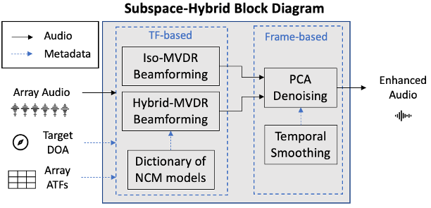
Fig. 1: The proposed system block diagram.

As illustrated in Fig. 1, the proposed method consists of two-stage multi-channel processing. In the first stage two types of beamforming are performed at every Time-Frequency (TF) bin. In the second stage, the spectrum output of both beamformers at each time frame are combined to form a two-channel data on which PCA [16] is performed to output the final enhanced signal. In addition to Iso-MVDR, described in Section 2.1, the system makes use of two novel processing blocks described as follows.

3.1 Hybrid-MVDR

This block, referred to as Hybrid, performs multiple MVDR beamforming with the same steering vector for a known target direction but various NCMs taken from a dictionary of pre-defined noise sound field models. The dictionary denoted as $P=\{{\mathbf{w}}_{m}({f},\Omega)\}$ contains the pre-calculated beamformer weights for each sample noise field model $m$, frequency index ${f}$ and steering direction $\Omega$ where $1\leq m\leq{M}$ for a total number of ${M}$ models. The output with the minimum power among the models is selected and denoted as

$${Y}_{\text{Hyb}}=({\mathbf{w}}_{j})^{H}{\mathbf{x}},$$ (8)

$$\mathrm{with\quad} j=\operatorname*{arg\,min}_{m}{\{\lVert({\mathbf{w}}_{m})^{H}{\mathbf{x}}\rVert^{2}\}}.$$ (9)

The dictionary can contain beamformer weights based on a variety of noise field models such as isotropic, anisotropic, Plane-Waves, spatially uncorrelated (diagonal covariance), and potentially more complex ones such as combination of basic ones or previously measured NCMs. The size and the models used in the dictionary are described in Section 3.3.

As will be shown in Section 4, although Hybrid beamformer results in stronger acoustic noise reduction, the output contains ‘musical noise’ due to rapid switching of beam pattern caused by potential selection of highly different models for neighbouring time frames and frequencies. To suppress this musical noise, which is assumed to be uncorrelated, or only partially correlated, with the acoustic noise, the next proposed block extracts that component of Hybrid-MVDR output which is correlated with the Iso-MVDR output.

3.2 Spectral PCA Denoising

In each time frame, let ${\mathbf{y}}({\tau})=[{Y}({\tau},1)\ldots{Y}({\tau},{F})]^{T}$ denote the spectrum output for a beamformer with a total of ${F}$ frequency bands. The associated outputs from Hybrid and Iso beamformers (identified by subscript) are joint to form a two-channel complex-value array of data

$${\mathbf{Z}}({\tau})=[{\mathbf{y}}_{\text{Hyb}}({\tau}),{\mathbf{y}}_{\text{Iso}}({\tau})].$$ (10)

The $2\times 2$ inter-channel covariance matrix of ${\mathbf{Z}}({\tau})$ is then

$${\mathbf{R}}({\tau})=\mathbb{E}\{{\mathbf{Z}}^{H}({\tau}){\mathbf{Z}}({\tau})\},$$ (11)

which can be approximated, using EMA, as

$${\mathbf{R}}_{\text{Z}}({\tau})=\alpha{\mathbf{R}}_{\text{Z}}({\tau}-1)+(1-\alpha)({\mathbf{Z}}^{H}({\tau}){\mathbf{Z}}({\tau})).$$ (12)

Using EigenValue Decomposition (EVD), ${\mathbf{R}}_{\text{Z}}$ is decomposed as

$${\mathbf{R}}_{\text{Z}}({\tau})={\mathbf{U}}({\tau}){\mathbf{\Sigma}}({\tau}){\mathbf{U}}^{-1}({\tau}),$$ (13)

where ${\mathbf{U}}\in\mathbb{C}^{2\times 2}$ and ${\mathbf{\Sigma}}$ are respectively the eigenvectors and diagonal matrix of eigenvalues. Assuming the columns of ${\mathbf{\Sigma}}$ are sorted in descending order of eigenvalues, the first column of $\mathbf{U}({\tau})=[\mathbf{U}_{S}({\tau}),\mathbf{U}_{N}({\tau})]$ is considered as signal eigenvector denoted as $\mathbf{U}_{S}({\tau})\in\mathbb{C}^{2\times 1}$.

The Signal Subspace (SS) of the ${\mathbf{Z}}({\tau})$ is reconstructed as

$${\mathbf{Z}}_{\text{SS}}({\tau})={\mathbf{Z}}({\tau}){\mathbf{U}}_{S}({\tau}){\mathbf{U}}_{S}^{H}({\tau}),$$ (14)

where the first column of ${\mathbf{Z}}_{\text{SS}}({\tau})=[{\mathbf{y}}_{\text{SS-Hyb}}({\tau}),{\mathbf{y}}_{\text{SS-Iso}}({\tau})]$ is considered as the final spectrum output of the system and denoted as ${\mathbf{y}}_{\text{SS-Hyb}}$.

3.3 Dictionary composition

Two variations of dictionary $P$, in Hybrid are considered using available ATFs. In the first version, denoted as SS-Hyb, the NCM models consist of the identity matrix, spherically isotropic noise and five unimodal anisotropic distributions across horizon, as shown in Fig. 2, horizontally rotated for every $6\text{\,}\deg$ azimuth spacing as for the peak position and were quadrature weighted along the inclination to form the 3D sound field. For unimodal anisotropic models, the power was a linear function of azimuth with power dynamic ranges of $\{8,16,24,32,40\}$\text{\,}\mathrm{dB}$$. The second version, denoted as SS-HybX, extends the number of models in the dictionary by additionally including individual PW models for all available ATF directions.

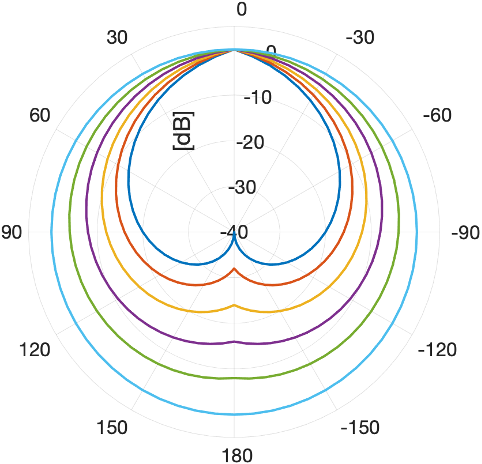
Fig. 2: Isotropic and five unimodal anisotropic models for the horizontal isotropy of the noise field.

4 Evaluations

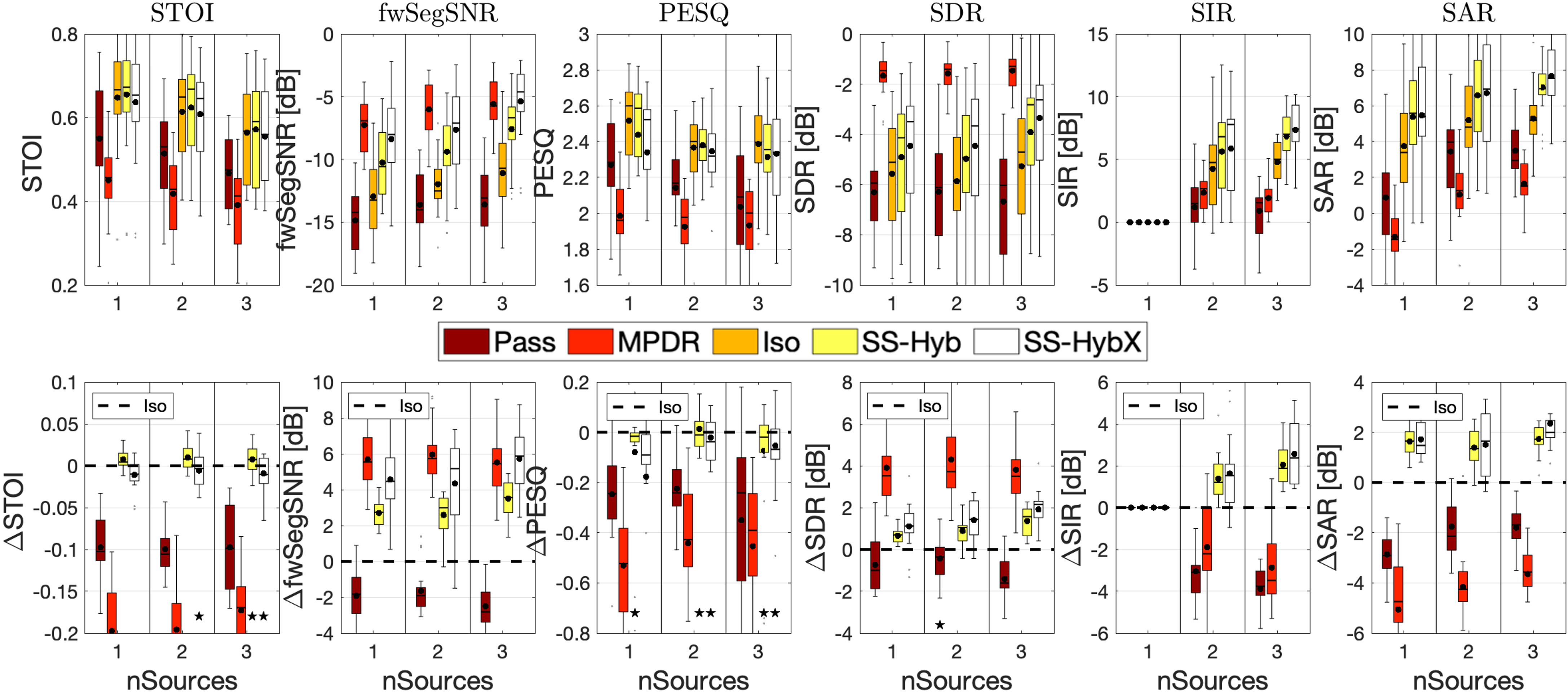
Fig. 3: The absolute (top) and relative (bottom) STOI [17], fwSegSNR [18], PESQ [19], SDR [20], SIR [20] and SAR [20].

In this section, the two implementations of the proposed method are compared with the Iso-MVDR and adaptive MPDR baseline beamformers as well as the ‘passthrough’ signal at the reference microphone.

4.1 Dataset and Array

In the context of augmented hearing and augmented reality, the EasyCom dataset [21] was used for evaluation. It contains recordings of ‘cocktail-party’ scenarios where a subject with 6-channel head-worn array (four microphones fixed to a pair of glasses and two positioned in the ears) was sat down with multiple talkers at a table surrounded by ten loudspeakers playing restaurant-like ambient noises. The target DOA over time is provided via head-tracking metadata for each talker. For this evaluation, the dataset is split into $6\text{\,}\mathrm{s}$ chunks such that the target onset occurs after $2\text{\,}\mathrm{s}$ based on the voice activity metadata in [21]. For the results visualization, the chunks were categorized according to the number of active sources per chunk denoted as ‘nSources’ = $[1,2,3]$. Close-talking headset microphones for each talker, also included in [21], were time- and level-aligned to the array reference microphone for use in intrusive metrics.

To avoid spatial aliasing due to the array geometry, data was down-sampled to $10\text{\,}\mathrm{kHz}$ sample rate. The Short Time Fourier Transform (STFT) used $16\text{\,}\mathrm{ms}$ time-window and $8\text{\,}\mathrm{ms}$ step. The smoothing factor $\alpha$ in (7) and (12) was chosen empirically with $T=$50\text{\,}\mathrm{ms}$$ and $T=$80\text{\,}\mathrm{ms}$$, respectively, for MPDR and SS-Hybrid. The condition number of the ${\mathbf{R}}$ for PWs in the dictionary of SS-HybX was limited to maximum of $100$ via NCM diagonal loading to avoid ill-condition covariance matrices. Our investigation showed no necessity of condition number limiting for the other NCM models, at least for this dataset.

4.2 Results and Discussions

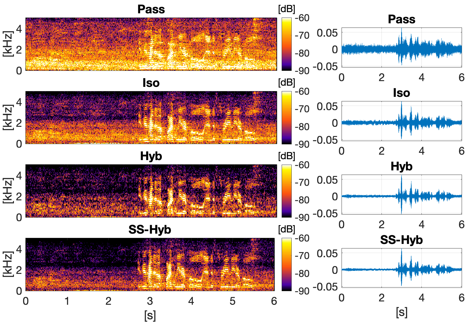
Fig. 4: Spectrograms of the methods for a trial (nSources=$1$).

Some audio examples of the results and animated visualization of the beam patterns are available at [22]. Figure 3 shows the absolute (top row) and relative (bottom row) performance according to various intrusive metrics. The black dot indicates the mean while a star indicates no significant difference from the Iso-MVDR (dashed line) according to paired t-test at $p=5\%$ level.

It can be seen that SS-Hyb outperforms the best baseline (Iso) by an average of $0.01$ STOI, $3\text{\,}\mathrm{dB}$ fwSegSNR, $1.5\text{\,}\mathrm{dB}$ SDR, $2\text{\,}\mathrm{dB}$ SIR, $1.8\text{\,}\mathrm{dB}$ SAR while sharing the best PESQ with Iso. On the other hand, SS-HybX performs better than SS-Hyb in noise suppression with additional mean of $2\text{\,}\mathrm{dB}$ fwSegSNR, $1\text{\,}\mathrm{dB}$ SDR, SIR and SAR particularly in the presence of interferer talker(s) (nSource$>1$), due to utilization of PW models, while sharing the same STOI and PESQ with Iso. Although MPDR provides the highest noise suppression, substantial target distortion caused by proneness to imperfection in target ATFs and DOA leads to poor STOI, PESQ, SIR and SAR scores.

Figure 4 shows the spectrograms of Passthrough, Iso, Hybrid and SS-Hybrid for a representative trial. Although Hybrid provides more noise suppression than Iso, it contains noticeable musical noise, which is suppressed in SS-Hybrid via PCA.

5 Conclusions

A novel two-stage multi-channel speech enhancement method is proposed which combines the robustness and computational simplicity of signal-independent beamforming with the performance of adaptive beamforming. The system proposes a Hybrid beamformer which performs multiple MVDR beamformers with different noise field models including isotropic and a variety of anisotropic distributions. The outputs from an Iso and optimal Hybrid beamformers are then jointly used to remove the musical noise via multi-channel PCA denoising. The evaluation results, using real-recording ‘cocktail-party’ scenario with head-worn microphone array, demonstrate the benefit of the proposed method in term of improved noise suppression and speech intelligibility with similar speech quality metric, compared to the baseline static and adaptive beamformers.

References

- [1] S. Doclo, S. Gannot, et al., “Acoustic beamforming for hearing aid applications,” in Handbook on Array Processing and Sensor Networks, S. Haykin and K. J. R. Liu, Eds., pp. 269–302. John Wiley & Sons, Inc., 2010.
- [2] H. W. Löllmann, A. H. Moore, et al., “Microphone array signal processing for robot audition,” in Proc. Joint Workshop on Hands-Free Speech Communication and Microphone Arrays (HSCMA), San Francisco, CA, USA, Mar. 2017, pp. 51–55.
- [3] R. Haeb-Umbach, S. Watanabe, et al., “Speech processing for digital home assistants: Combining signal processing with deep-learning techniques,” IEEE Signal Processing Magazine, vol. 36, no. 6, pp. 111–124, Nov 2019.
- [4] Y. Liu, A. Ganguly, et al., “Neural network based time-frequency masking and steering vector estimation for two-channel mvdr beamforming,” in IEEE International Conference on Acoustics, Speech and Signal Processing (ICASSP). Apr 2018, IEEE.
- [5] H. Erdogan, J. R. Hershey, et al., “Improved MVDR beamforming using single-channel mask prediction networks.,” in Proc. Interspeech, 2016, pp. 1981–1985.
- [6] J. Bitzer and K. U. Simmer, “Superdirective microphone arrays,” in Microphone Arrays: Signal Processing Techniques and Applications, M. Brandstein and D. Ward, Eds., Digital Signal Processing, pp. 19–38. Springer, Berlin, Heidelberg, 2001.
- [7] H. L. van Trees, Detection, Estimation, and Modulation Theory, vol. IV, Optimum Array Processing, John Wiley & Sons, Inc., New York, USA, Apr. 2002.
- [8] J. Capon, “High-resolution frequency-wavenumber spectrum analysis,” Proc. IEEE, vol. 57, no. 8, pp. 1408–1418, Aug. 1969.
- [9] H. Cox, “Resolving power and sensitivity to mismatch of optimum array processors,” J. Acoust. Soc. Am., vol. 54, no. 3, pp. 771–785, Sept. 1973.
- [10] L. Ehrenberg, S. Gannot, et al., “Sensitivity analysis of MVDR and MPDR beamformers,” in IEEE Conv. Electrical and Electronics Engineers, Eilat, Israel, Nov. 2010, pp. 416–420.
- [11] S. Gannot, E. Vincent, et al., “A consolidated perspective on multimicrophone speech enhancement and source separation,” IEEE/ACM Trans. Audio, Speech, Language Process., vol. 25, no. 4, pp. 692–730, Apr. 2017.
- [12] E. C. Cherry, “Some experiments on the recognition of speech, with one and with two ears,” J. Acoust. Soc. Am., vol. 25, no. 5, pp. 975–979, Sept. 1953.
- [13] J. Zhang, R. Heusdens, and R. C. Hendriks, “Relative acoustic transfer function estimation in wireless acoustic sensor networks,” IEEE/ACM Transactions on Audio, Speech, and Language Processing, vol. 27, no. 10, pp. 1507–1519, Oct 2019.
- [14] O. Schwartz, S. Gannot, and E. A. P. Habets, “An Expectation-Maximization Algorithm for Multimicrophone Speech Dereverberation and Noise Reduction With Coherence Matrix Estimation,” IEEE/ACM Transactions on Audio, Speech, and Language Processing, vol. 24, no. 9, pp. 1495–1510, Sept. 2016.
- [15] J. R. Driscoll and D. M. Healy, “Computing Fourier transforms and convolutions on the 2-sphere,” Advances in Applied Mathematics, vol. 15, no. 2, pp. 202–250, June 1994.
- [16] I. T. Jolliffe, Principal Component Analysis, New York, 2002.
- [17] C. H. Taal, R. C. Hendriks, et al., “An algorithm for intelligibility prediction of time-frequency weighted noisy speech,” IEEE Trans. Audio, Speech, Language Process., vol. 19, no. 7, pp. 2125–2136, Sept. 2011.
- [18] Y. Hu and P. C. Loizou, “Evalution of objective quality measures for speech enhancement,” IEEE/ACM Trans. Audio, Speech, Language Process., vol. 16, no. 1, Jan. 2008.
- [19] A. Rix, J. Beerends, et al., “Perceptual evaluation of speech quality (PESQ)-a new method for speech quality assessment of telephone networks and codecs,” in Proc. IEEE Int. Conf. on Acoust., Speech and Signal Process. (ICASSP), Salt Lake City, UT, USA, May 2001, vol. 2, pp. 749–752.
- [20] E. Vincent, R. Gribonval, and C. Févotte, “Performance measurement in blind audio source separation,” IEEE Trans. Audio, Speech, Language Process., vol. 14, no. 4, pp. 1462–1469, July 2006.
- [21] J. Donley, V. Tourbabin, et al., “EasyCom: An Augmented Reality Dataset to Support Algorithms for Easy Communication in Noisy Environments,” arXiv:2107.04174 [cs, eess], Oct. 2021.
- [22] “SS-Hybrid audio demo [online],” https://imperialcollegelondon.github.io/sap-SSHybrid-demo/.