Ms.FPOP: An Exact and Fast Segmentation Algorithm With a Multiscale Penalty

Abstract

Given a time series in $\mathbb{R}^{n}$ with a piecewise constant mean and independent noises, we propose an exact dynamic programming algorithm to minimize a least square criterion with a multiscale penalty promoting well-spread changepoints. Such a penalty has been proposed in Verzelen et al. (2020), and it achieves optimal rates for changepoint detection and changepoint localization.

Our proposed algorithm, named Ms.FPOP, extends functional pruning ideas of Rigaill (2015) and Maidstone et al. (2017) to multiscale penalties. For large signals, $n\geq 10^{5}$, with relatively few real changepoints, Ms.FPOP is typically quasi-linear and an order of magnitude faster than PELT. We propose an efficient C++ implementation interfaced with R of Ms.FPOP allowing to segment a profile of up to $n=10^{6}$ in a matter of seconds.

Finally, we illustrate on simple simulations that for large enough profiles ($n\geq 10^{4}$) Ms.FPOP using the multiscale penalty of Verzelen et al. (2020) is typically more powerfull than FPOP using the classical BIC penalty of Yao 1989.

1 Introduction

A National Research Council report [1] identifies changepoint detection as one of the “inferential giants” in massive data analysis. Detecting changepoints, whether a posteriori or online, is important in areas as diverse as bioinformatics [2, 3], econometrics and finance [4, 5], climate [6], autonomous driving [7], computer vision [8] and neuroscience [9]. The most common and prototypical changepoint detection problem is that of detecting changes in mean of a univariate gaussian signal :

$$y_{t}=f_{t}+\varepsilon_{t},\quad\text{for }t=1,\ldots,n,$$ (1)

where $f_{t}$ is a deterministic piecewise constant with changepoints whose number $D$ and locations, $0<\tau_{1}<\ldots<\tau_{D}<n$, are unknown, and $\varepsilon_{t}$ are independant and follow a Gaussian distribution of mean 0 and variance 1. A large number of approaches have been proposed to solve this problem (amongst many others [10, 11, 12, 13, 14], see [15, 16] for a review).

Recently, [17] characterize optimal rates for changepoint detection and changepoint localization and proposed a least-squares estimator with a multiscale penalty achieving these optimal rates. This multiscale penalty depends on minus the log-length of the segments which promotes well spread changepoints. It can be written as :

$$\sum_{d=1}^{D+1}\gamma+\beta\log(n)-\beta\log(\tau_{d}-\tau_{d-1}),$$ (2)

where $\gamma=qL$ and $\beta=2L$ with $q$ positive and $L>1$, and with the convention that $\tau_{0}=0$ and $\tau_{D+1}=n$.

Up to a multiplicative constant this penalty is always smaller than the BIC penalty ($2\log(n)$) [10]. Intuitively, it favors balanced segmentation as:

• the penalty of a fixed sized segment ($r$) increases with $n$ : $\beta\log(n/r).$

• while the penalty for a segment whose size is proportionnal to $n$ ($\alpha.n$) is constant of $n$ : $\beta\log(1/\alpha).$

Contribution

In this paper, we propose a dynamic programming algorithm, named Ms.FPOP optimizing a slightly more general penalty. where the $\log(\tau_{d}-\tau_{d-1})$ is replaced by $g(\tau_{d}-\tau_{d-1})$ for an arbitrary function $g$ satistying assumption A1.

Existing works

Ms.FPOP extends functional pruning techniques as in PDPA or FPOP [18, 19] to the case of multiscale penalties. A key condition for FPOP and PDPA is that the cost function is point additive (condition C1 in [19]). As we will explain in more details later, this condition is not verified for the multiscale penalty (2), making the extension not trivial. The key idea behind functionnal pruning is to store the set of parameter values for which a particular change is optimal. For a classical penalty (i.e. with a point additive cost function) this set gets smaller with every new datapoint. This is not the case with the multiscale penalty making the update more complex. A key insight of Ms.FPOP is to store a slightly larger set that is easy to update.

Importantly, it is possible to optimize the multiscale criteria of [17] using inequality based pruning as in PELT. We will call Ms.PELT this strategy. However for large signals with relatively few true changepoints it is our experience that Ms.PELT is quadratic while Ms.FPOP is quasi-linear. For example it can be seen on Figure 1.A that it takes about 193 seconds for Ms.PELT to process a signal of size $n=128000$ without any changepoint. In the same amount of time Ms.FPOP can process signals of size larger than $n=4\times 10^{6}.$ In the presence of true changepoints, (one every thousand datapoints) Ms.PELT as expected is much faster but still slower than Ms.FPOP (see Figure 1.B).

Figure 1: Runtimes of PELT and Ms.FPOP as a function of $n$ to optimize the multiscale penalty of [17] with $\beta=2.25$ and $q=9$ on an Intel Core i7-10810U CPU @ 1.10GHzx12 computer for signals without changes (A) or signal with a change of size 1 every thousand datapoints (B).

Outline

In the rest of the paper we will (1) introduce our notations, (2) review the key idea behind FPOP, (3) explain how and under which conditions we extend FPOP to multiscale penalty, (4) study the performance of Ms.FPOP relative to FPOP for various signals and (5) conclude with a discussion.

1.1 Multiple Changepoint Model

In this section we describe our changepoint notations and the multiscale criteria we want to optimize.

Segmentations and set of segmentations

For any $n$ in $\mathbb{N}$ we write $1:n=\{1,\cdots,n\}$. For any integer $D\geq 0$ we define a segmentation with $D$ changes of $1:n$ as an ordered subset of $1:(n-1)$ of size $D,$ with $\tau_{j}$ the location of the $j^{th}$ change for $j$ in $1,\ldots,D$. It will be usefull to also consider the dummy indices $\tau_{0}=0$ and $\tau_{D+1}=n$. We call $\mathcal{M}^{D}_{1:n}$ the set of all such segmentations in $D$ changes and $\mathcal{M}_{1:n}$ the union of all these sets : $\bigcup_{0\leq D\leq n-1}\mathcal{M}^{D}_{1:n}.$ For any segmentation $\tau$ in $\mathcal{M}_{1:n}$ we note $|\tau|$ the number of segments of $\tau$. In other words, if $\tau$ is in $\mathcal{M}^{D}_{1:n}$ then $|\tau|=D+1.$ We can enumerate the elements of $\mathcal{M}_{1:n}$ and we get :

$$|\mathcal{M}_{1:n}|=\sum_{D=0}^{n-1}|\mathcal{M}^{D}_{1:n}|=\sum_{D=0}^{n-1}\binom{n-1}{D}=2^{n-1}$$

Multiscale penalized likelihood

Under the piecewise constant model 1 a classical method to estimate the position and the number of changes is to optimize a penalized likelihood criterion. It is common to use a penalty that is linear in the number of changepoints [10, 20, 19] and optimization wise the goal is to compute:

$${\Large{\boldsymbol{\tau}}}^{*}_{n} = \operatorname*{arg\,min}_{\tau\in\mathcal{M}_{1:n}}\ \left\{\displaystyle\sum_{j=1}^{|\tau|}\min_{\mu}\left(\displaystyle\sum_{i=\tau_{j-1}+1}^{\tau{j}}(y_{i}-\mu)^{2}\right)+\alpha|\tau|\right\},$$

$$F_{n} = \min_{\tau\in\mathcal{M}_{1:n}}\ \left\{\displaystyle\sum_{j=1}^{|\tau|}\min_{\mu}\left(\displaystyle\sum_{i=\tau_{j-1}+1}^{\tau{j}}(y_{i}-\mu)^{2}\right)+\alpha|\tau|\right\},$$

(3)

where $\alpha$ is a constant to be calibrated (e.g. $\alpha=2\log(n)$).

Here we consider a more general penalty that depends on the length of the segments:

$${\Large{\boldsymbol{\tau}}}^{*}_{n} = \operatorname*{arg\,min}_{\tau\in\mathcal{M}_{1:n}}\ \left\{\displaystyle\sum_{j=1}^{|\tau|}\min_{\mu}\left(\displaystyle\sum_{i=\tau_{j-1}+1}^{\tau{j}}(y_{i}-\mu)^{2}-\beta g(\tau_{j}-\tau_{j-1})\right)+\alpha|\tau|\right\},$$

$$F_{n} = \min_{\tau\in\mathcal{M}_{1:n}}\ \left\{\displaystyle\sum_{j=1}^{|\tau|}\min_{\mu}\left(\displaystyle\sum_{i=\tau_{j-1}+1}^{\tau{j}}(y_{i}-\mu)^{2}-\beta g(\tau_{j}-\tau_{j-1})\right)+\alpha|\tau|\right\},$$

(4)

where $g$ is a function satistfying assumption A1 described in the next paragraph, and $\alpha$ and $\beta$ are constants to be calibrated. We recover the multiscale criteria proposed in [17] taking $g=\log$, $\alpha=\gamma+\beta g(n)$, and $\gamma$ a constant that remains to be chosen. We recover the classical penalty of [10] taking $g=0$, $\alpha=2\log(n).$

Assumption 1.

$h(t,s,s^{\prime})=g(t-s^{\prime})-g(t-s)$ is a non-decreasing function in $t$, and $\lim_{t\to\infty}h(t,s,s^{\prime})=0$ therefore $h(t,s,s^{\prime})\leq 0$.

This assumption will be useful later to bound the difference between the cost of two changes $s$ and $s^{\prime}$. Intuitively, assumption A1 states that $g$ favors older changes but that asymptotically (large enough $t$ relative to $s$ and $s^{\prime}$) this advantage for older changes vanishes. Importantly, this assumption is true for the multiscale penalty proposed in [17] as $\beta>0$ and $g(t-s^{\prime})-g(t-s)=\log(1-(s^{\prime}-s)/(t-s))$ is increasing with $t$.

1.2 Optimization with Dynamic Programming

In this section we explain how one can optimize equation (4) using dynamic programming ideas with (i) inequality based pruning and (ii) functional pruning.

Dynamic programming with inequality based pruning

The penalised cost of a segmentation $\tau$ inside the $\arg\min$ of equation (4) can be written as a sum over all segments of $\tau$ :

$$\sum_{j=1}^{|\tau|}\min_{\mu}\left(\displaystyle\sum_{i=\tau_{j-1}+1}^{\tau{j}}(y_{i}-\mu)^{2}-\beta g(\tau_{j}-\tau_{j-1})+\alpha\right),$$

therefore the optimisation can be done iteratively using the Optimal Partionning (OP) algorithm proposed in [21] using dynamical programming ideas developped in [22] and [23]. It is possible to speed calculations using the PELT  algorithm [20] because equation (4) of [20] is true at least for constant $K=-\beta(\max_{1\leq\ell\leq n}\{g(\ell)\}-2\min_{1\leq\ell\leq n}\{g(\ell)\})$ (see A). If $g$ is concave (as in the penalty (2) proposed in [17]), $K$ can be chosen much closer to zero : $K=-\beta(g(2)-2g(1))$ (see A), or adaptively to the last segment length $\ell$ : $\ K_{\ell}=-\beta(g(\ell)+g(1)-g(\ell+1))$ (see B). Our implementation of PELT optimizing (4) with $g=\log$ and $K_{\ell}=-\beta\log(\frac{1}{\ell}+1)$ is called Ms.PELT. Note that $K_{\ell}\leq-\beta\log(2)$.

As shown in the Figure 1, if the number of real changepoints is not linear in $n$, for $g=\log$, and a positive $\beta$, Ms.PELT is quadratic. This makes the analysis of large profiles with $10^{5}$ or $10^{6}$ datapoints long and unpractical (e.g. $>100$ seconds for a profile with $10^{5}$ datapoints and 1 changepoint, $>1$ hour for a profile with $10^{6}$ datapoints and 1 changepoint ).

Dynamic programming with functional pruning

In the rest of the paper, we present a functional pruning algorithm (called Ms.FPOP), in the sense of the PDPA [18] or FPOP [19], to solve (4), making it possible to optimize (4) in a matter of seconds even for $n=10^{6}$ As the cost of equation (4) is not point-additive, condition C1 of [19] is not true, and maintaining the set of means for which a change is optimal is more complex. Our key idea is to maintain a slightly larger set that is easier to update.

2 Functional Pruning

2.1 Functional Pruning Optimal Partioning (FPOP)

To better explain Ms.FPOP we first review some of the key elements of FPOP to optimize equation (3). FPOP introduces for every change $s$ its best cost as function of the last parameter $\mu$ at time $t$, $\widetilde{f}_{t,s}(\mu)$. Formally this is:

$$\widetilde{f}_{t,s}(\mu)=F_{s}+\displaystyle\sum_{i=s+1}^{t}(y_{i}-\mu)^{2}+\alpha,\text{ }\text{ }\text{ with }\text{ }\text{ }\widetilde{f}_{t,t}(\mu)=F_{t}+\alpha\text{ }\text{ }\text{ and }\text{ }\text{ }F_{0}=-\alpha.$$ (5)

$\widetilde{f}_{t,s}(\mu)$ is a second degree polynomial in $\mu$ defined by three coefficients : $a_{2}\mu^{2}+a_{1}\mu+a_{0}$ with $a_{2}=t-s,$ $a_{1}=-2\sum_{i=s+1}^{t}y_{i}$ and $a_{0}=F_{s}+\alpha+\displaystyle\sum_{i=s+1}^{t}y_{i}^{2}$. The update of these coefficients is straightforward using the following formula:

$$\widetilde{f}_{t,s}(\mu)=\widetilde{f}_{t-1,s}(\mu)+(y_{t}-\mu)^{2}.$$ (6)

At each time step $t$, FPOP updates the minimum of all $\widetilde{f}_{t,s}(\mu)$, denoted $\widetilde{F}_{t}(\mu)=\min_{s\leq t}\ \left\{\widetilde{f}_{t,s}(\mu)\right\}.$ The key idea behind FPOP is that to compute and update $\widetilde{F}_{t}(\mu)$ one only need to consider changes $s$ with a none empty “living-set” : $\mathcal{F}_{t}=\{s\leq t|Z_{t,s}^{*}\neq\emptyset\}$ where the “living-set” of change $s$ is $Z_{t,s}^{*}=\{\mu|\widetilde{f}_{t,s}(\mu)=\widetilde{F}_{t}(\mu)\}$. Given those definitions we have $\widetilde{F}_{t}(\mu)=\min_{s\in\mathcal{F}_{t}}\ \left\{\widetilde{f}_{t,s}(\mu)\right\}$. In other words, $s$ is pruned as soon as its “living-set” is empty, which is justified because

$$Z_{t,s}^{*}\supset Z_{t+1,s}^{*}.\text{ }\text{ }\text{ }\text{and }\text{ }\text{ }\text{ }Z_{t,s}^{*}=\emptyset\implies Z_{t+1,s}^{*}=\emptyset\ .$$ (7)

Note that we can then retrieve $F_{t}$ by minimizing $\widetilde{F}_{t}(\mu)$ on $\mu$.

2.2 Ms.FPOP : functional Pruning for a Multiscale Penalty

Ms.FPOP optimizes equation (4). As for FPOP we introduce for every change $s$ its best cost as a function of the last parameter $\mu$ at time $t$, $\widetilde{f}_{t,s}(\mu)$. Formally this is :

$$\widetilde{f}_{t,s}(\mu)=F_{s}+\displaystyle\sum_{i=s+1}^{t}(y_{i}-\mu)^{2}+\alpha-\beta g\left(t-s\right),$$ (8)

with $\widetilde{f}_{t,t}(\mu)=F_{t}+\alpha$ and $F_{0}=-\alpha$. As in FPOP, $\widetilde{f}_{t,s}(\mu)$ can be stored as a second degree polynomial in $\mu$. The update is also straightforward using the following formula:

$$\widetilde{f}_{t,s}(\mu)=\widetilde{f}_{t-1,s}(\mu)+(y_{t}-\mu)^{2}+\beta g\left(t-1-s\right)-\beta g\left(t-s\right)$$ (9)

Analogously to FPOP we can calculate $F_{t}$ by minimizing $\widetilde{f}_{t,s}$ both on $\mu$ and $s$. The main difference with FPOP is that the rule (7) is no longer true for Ms.FPOP because $\widetilde{f}_{t,s}(\mu)-\widetilde{f}_{t,s^{\prime}}(\mu)$ depends on $t$:

$$\widetilde{f}_{t,s}(\mu)-\widetilde{f}_{t,s^{{}^{\prime}}}(\mu)=F_{s}-F_{s^{{}^{\prime}}}+\displaystyle\sum_{i=s+1}^{s{{}^{\prime}}}(y_{i}-\mu)^{2}+\beta(\underbrace{g(t-s^{{}^{\prime}})-g(t-s))}_{\begin{subarray}{c}\text{{a function varying}}\\ \text{{with t, s et s'}}\end{subarray}}).$$ (10)

Because of that, in the course of the algorithm we need to re-evaluate the set on which the candidate change $s$ is better than $s^{\prime}$ at various $t$, $I_{t,s,s^{{}^{\prime}}}$ with $s<s^{{}^{\prime}}$:

$$I_{t,s,s^{{}^{\prime}}}=\{\mu\ |\ \widetilde{f}_{t,s}(\mu)\ \leq\ \widetilde{f}_{t,s^{{}^{\prime}}}(\mu)\}.$$ (11)

For arbitrary functions $g$ the set $I_{t,s,s^{{}^{\prime}}}$ may vary drastically from one $t$ to the next. Using assumption A1 we can control those variations.

2.2.1 Update of The Candidate Changes Living Set ($Z_{t,s}$)

Rather than evaluating the exact living set $Z_{t,s}^{*}$ of all changes, we are seeking to update a slightly larger set, $Z_{t,s}$, including $Z_{t,s}^{*}$ and such that if $Z_{t,s}$ is empty we can guarantee that $Z_{t+h,s}^{*}$ is also empty for all $h>0$. The possibility of defining such a $Z_{t,s}$ depends on the property of the function $g$.

Assume A1 we propose to update $Z_{t+1,s}$ as follow:

$$Z_{t+1,s}=Z_{t,s}\ \cap\overbrace{(\ \bigcap_{s^{\prime}\in\mathcal{A}_{t,s}}I_{t+1,s,s{{}^{\prime}}})}^{\text{{comparison with future changes}}}\backslash\overbrace{(\ \bigcup_{s^{\prime\prime}\in\mathcal{B}_{s}}I_{\infty,s{{}^{\prime\prime}},s})}^{\text{{comparison with past changes}}}\ ,$$ (12)

where $\mathcal{A}_{t,s}$ is any subset of $\{s+1,...,t\}$, $\mathcal{B}_{s}$ is any subset of $\{1,...,s-1\}$, and $I_{\infty,s,s^{{}^{\prime}}}$ correspond to $I_{t,s,s^{{}^{\prime}}}$ when $t\to\infty$ (which is properly define under assumption A1).

Pruning

Based on update (12) it should be clear that if $Z_{t,s}$ is empty so are all $Z_{t+h,s},$ for $h>0.$ In the next lemma we show that $Z_{t,s}$ includes $Z^{*}_{t,s}.$ Therefore we further have that if $Z_{t,s}$ is empty so are all $Z^{*}_{t+h,s},$ and change $s$ can be pruned.

Lemma 1.

Taking $Z_{s,s}=]min_{i}y_{i},\max_{i}y_{i}[$, updating $Z_{t+1,s}$ using equation (12) and assuming A1 we have

$$Z_{t,s}^{*}\subset Z_{t,s}\ ,$$ (13)

and for an integer $h>0$

$$Z_{t+h,s}^{*}\subset Z_{t+1,s}\ .$$ (14)

Proof.

For any $t$, we will prove by induction that for any $t^{\prime}$ in $\{s,\cdots,t\}$ we have $Z_{t,s}^{*}\subset Z_{t^{\prime},s}.$

For $t^{\prime}=s$ and for any $t$ larger or equal to $s$ we have (by definition of $Z_{s,s}$) that $Z_{t,s}^{*}\subset Z_{t^{\prime},s}=Z_{s,s}.$

Now assume that for $t^{\prime}<t$ we have $Z_{t,s}^{*}\subset Z_{t^{\prime},s}.$ As $h$ is non-decreasing for any $t^{\prime}+1\leq t$ we have the following two inclusions :

$$I_{t,s,s^{{}^{\prime}}} \subset I_{t^{\prime}+1,s,s^{{}^{\prime}}}.$$ (15)

$$I_{\infty,s,s^{{}^{\prime}}} \subset I_{t^{\prime}+1,s,s^{{}^{\prime}}}$$ (16)

Therefore for $t^{\prime}<t$ we have

$$Z^{*}_{t,s} = \qquad\quad(\ \bigcap_{s<s^{{}^{\prime}}\leq t}I_{t,s,s^{{}^{\prime}}})\backslash(\ \bigcup_{s^{{}^{\prime\prime}}<s}I_{t,s{{}^{\prime\prime}},s})\qquad\quad\quad\text{ by definition of }Z^{*}_{t,s}$$

$$Z^{*}_{t,s} \subset Z_{t^{\prime},s}\ \cap(\ \bigcap_{s<s^{{}^{\prime}}\leq t}I_{t,s,s^{{}^{\prime}}})\backslash(\ \bigcup_{s^{{}^{\prime\prime}}<s}I_{t,s{{}^{\prime\prime}},s})\qquad\quad\quad\text{by induction}$$

$$\subset Z_{t^{\prime},s}\ \cap(\ \bigcap_{s\ <s^{{}^{\prime}}\leq\ t}I_{t^{\prime}+1,s,s^{{}^{\prime}}})\backslash(\ \bigcup_{s^{{}^{\prime\prime}}<\ s}I_{\infty,s^{{}^{\prime\prime}},s})\quad\text{using equation \eqref{inclus2} and\eqref{inclus1}}$$

$$\subset Z_{t^{\prime},s}\ \cap(\ \bigcap_{s^{{}^{\prime}}\in\ \mathcal{A}_{t^{\prime},s}}I_{t^{{}^{\prime}}+1,s,s^{{}^{\prime}}})\backslash(\ \bigcup_{s^{{}^{\prime\prime}}\in\ \mathcal{B}_{s}}I_{\infty,s^{{}^{\prime\prime}},s})\quad\text{by definition of }\mathcal{A}_{t^{\prime},s}\text{ and }\mathcal{B}_{s}.$$

Using equation (12) we thus get that $Z^{*}_{t,s}\subset Z_{t^{\prime}+1,s},$ proving the induction.

To recover equation (14) we notice from update (12) that $Z_{t+1,s}\subset Z_{t,s}$ and apply equation (13). ∎

2.2.2 Ms.FPOP Algorithm, Choice of $\mathcal{A}_{t,s}$ and $\mathcal{B}_{s}$

The update rule (12) suggest that for each candidate change $s$ we should compare it future change $s^{\prime}$ in $\mathcal{A}_{t,s}$, and past change $s^{\prime\prime}$ in $\mathcal{B}_{s}$. For past candidate changes $s^{{}^{\prime\prime}}$ this comparison can be done once and for all considering that $t$ goes to infinity ($I_{\infty,s^{{}^{\prime\prime}},s}$). For future candidate changes $s^{{}^{\prime}}$, on the contrary, it might be usefull to update the interval $I_{t,s,s^{{}^{\prime}}}$. Performing at each time step, for each $s$, a comparison with all s’ is time consuming. Intuitively, the complexity of each time step is in $\mathcal{O}(\text{number of candidate changes}^{2}).$ Ideally, for each $s$, one would like to make the minimum number of comparisons that would result in its pruning. In the Algorithm 1 we consider a generic sampling function of $s^{\prime}$ that returns $\mathcal{A}_{t,s}$ (see the Sampling Strategies paragraph in section 3).

Input: $Y=(y_{1},...,y_{n})$, $\ \alpha$,$\ \beta$, $\ g=log(.)$

Output: set of last best changes $cp_{n}$

1 $n\leftarrow|Y|$;

2 $F_{0}\leftarrow-\alpha$;

3 $cp_{0}\leftarrow\emptyset$;

4 $R_{1}\leftarrow\{0\}$;

5 $D\leftarrow[min(Y),\ max(Y)]$;

6 $Z_{0,0}\leftarrow D$;

7 $\widetilde{f}_{0,0}\leftarrow F_{0}+\alpha\ (=0)$;

8 for $t\leftarrow 1,...,n$ do

9       for $s\in R_{t}$ do

10             $\widetilde{f}_{t,s}(\mu)\leftarrow\widetilde{f}_{t,s}(\mu)+(y_{t}-\mu)^{2}+\beta\times g(t-1-s)-\beta\times g(t-s)$;

11            

12       end for

13      $F_{t}\leftarrow\min_{s\in R_{t}}(\operatorname*{min}_{\mu\in Z_{t,s}}(\widetilde{f}_{t,s}(\mu)))$;

14       $s_{t}\leftarrow\operatorname*{arg\,min}_{s\in R_{t}}(\min_{\mu\in Z_{t,s}}(\widetilde{f}_{t,s}(\mu)))$;

15       $cp_{t}\leftarrow(cp_{s_{t}},s_{t})$;

16       $\widetilde{f}_{t,t}\leftarrow F_{t}+\alpha$;

17       $Z_{t,t}\leftarrow D$;

18       for $s\in R_{t}$ do

19             $Z_{t,t}\leftarrow Z_{t,t}\ \backslash\ I_{\infty,s,t}$;

20             $\mathcal{A}_{t,s}\leftarrow sample(\{s^{{}^{\prime}}\in\{R_{t}\cup\{t\}\}:s^{{}^{\prime}}>s\})$;

21             $Z_{t,s}\leftarrow Z_{t,s}\cap(\bigcap_{s^{{}^{\prime}}\in\ \mathcal{A}_{t,s}}I_{t,s,s^{{}^{\prime}}})$;

22            

23       end for

24      $R_{t+1}\leftarrow\{s\in\{R_{t}\cup\{t\}\}:Z_{t,s}\neq\emptyset\}$;

25      

26 end for

Algorithm 1 Ms.FPOP

3 Rcpp Implementation of Ms.FPOP Algorithm

Ms.FPOP R package

The dynamic programming and functional pruning procedures describe in the algorithm 1 are implemented in C++. The input and output operations are interfaced with the R programming language thanks to Rcpp R package. The main function MsFPOP() takes as input the sequence of obervations, a vector of weights for these obervations, the parameters $\beta$ and $\alpha$ of the multiscale penalty. The function returns the set of optimal changepoints in the sense of (4). Analogously, we implemented a version of the PELT algorithm, MsPELT(), that optimizes (4).

Sampling Strategies

To recover $\mathcal{A}_{t,s}$ we consider either an exhaustive sampling of all future changes $s^{\prime}>s$ in $R_{t}$ or a uniform random subsampling of them without replacement. The main function parameter size can be set by the user to specify for each $s$ the number of sampled $s^{\prime}$. In the appendix we compare the runtime of different sampling strategies (see D).

4 Simultation Study

4.1 Calibration of Constants $\gamma$ and $\beta$ from The Multiscale Penalty

Paper [17] does not recommend values for $\gamma$ and $\beta$ in their penalty (2). As explained in detail below, we calibrated those values to control the percentage of falsely detecting at least one change in profiles simulated without any actual change.

No change simulation

We repeatedly simulate iid Gaussian signals of mean 0, variance 1 and varying lengths $n$ ($n\in\{10^{2},10^{3},10^{4},10^{5},2.5\times 10^{5}\}$). On these profiles we run Ms.FPOP for different $\gamma$ values (ten $\gamma$ values evenly spaced on the interval $[1,20]$) and different $\beta$ values ($\beta\in\{2,2.25,2.5,2.75,3\})$.

Percentage of false detection

We denote $R_{>0}$ as the proportion of replicates for which Ms.FPOP returns at least 1 changepoint. These changepoints are false positives. Our goal is to find a combination of $\beta$ and $\gamma$ such that

$$R_{>0}<0.05\ (\text{significance level})\quad.$$ (17)

Empirical Results

In Figure 2 we observe that, by setting $\beta=2.25$, a conservative range of $\gamma$ satisfying inequality (17) can be reached for $\gamma\in[7.5,10]$. Note that this interval satisfy inequality (17) for all tested $n$ and $\beta$ (see C).

Based on these results, in the following simulations we set $\gamma=9$ and $\beta=2.25$ for all methods optimizing (4) (Ms.FPOP, Ms.PELT). We set $\alpha=2\sigma^{2}\log(n)$ for all methods optimizing (3) (FPOP, PELT).

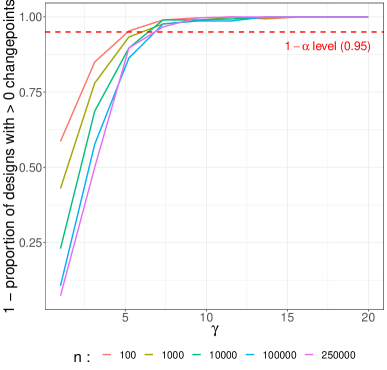
Figure 2: Proportion of stationary Gaussian signal replicates on which Ms.FPOP returns at least 1 changepoint ($R_{>0}$). $R_{>0}$ is computed for a series of $\gamma$ and profile lengths (see Design of Simulations). In these simulations we set $\beta=2.25$. Results for other $\beta$ values are availables in C.

4.2 Evalutation of Ms.FPOP: Speed Benchmark

Design of Simulations

We repeatedly simulate iid Gaussian signals with $10^{5}$ datapoints. The profiles are affected by one or more changepoints in their mean ($D\in\{1,5,10,15,20,25,30,45,50,100,150,200,250,300,350,400,450,$
$500,550,600,650,700,750,800,850,900,950,1000\}$). The mean of segments alternates between 0 and 1, starting with 0. The variance of each segment is fixed at 1. On these profiles we run two methods optimizing the penalized likelihood defines in (3): PELT [20] and FPOP [19], as well as methods optimizing the multiscale penalized likelihood defines in (4): Ms.PELT and Ms.FPOP. For Ms.FPOP, after comparisons with other sampling strategies (see D), we choose to randomly sample 1 future candidate change.

Metric

For each replicate we time in seconds the compared methods.

Empirical Results

In Figure 3 we firstly observe that for both criteria (multiscale penalized likelihood and penalized likelihood), functional pruning methods are always faster than inequality based pruning ones. Indeed, Ms.FPOP and FPOP are always faster than Ms.PELT and PELT, respectively. The smaller $D$, the larger the time difference between functional pruning methods and inequality based pruning ones. For $D=1$, Ms.FPOP runs in 2.4 seconds in average and is about 50 times faster than Ms.PELT (121.3 seconds in average). For $D=1000$, Ms.FPOP runs in 0.7 second in average and is about 1.3 times faster than Ms.PELT (0.9 second in average). Marginally to $D$, FPOP runs always under 0.05 seconds. Similar trends can be observed on iid Gaussian signals with $10^{6}$ datapoints (see Figure 8).

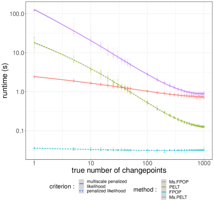
Figure 3: Runtimes as a function of the true number of changepoints. We timed PELT, Ms.PELT, FPOP, Ms.FPOP on profiles of length $n=10^{5}$ with varying number of true changepoints $D$ (see Design of Simulations) on an Intel Core i7-10810U CPU @ 1.10GHzx12 computer. The comparison between sampling strategies of future candidate changes implemented in Ms.FPOP is available in Figure 7. The comparison of PELT, FPOP, Ms.FPOP on profiles of length $n=10^{6}$ is available in Figure 8.

4.3 Evalutation of Ms.FPOP relative to FPOP: Accuracy Benchmarks

In this section we seek to illustrate using minimalist simulations the performances of the multiscale criteria proposed in [17] and implemented in Ms.FPOP relative to the BIC criteria proposed in [10] and implemented in FPOP.

4.3.1 Hat Simulations

Design of Simulations

We repeatedly simulate iid Gaussian signals of varying size $n\in\{10^{3},10^{4},10^{5}\}$. Each signal is affected by 2 changepoints. The second changepoint ($\tau_{2}$) is fixed at position $\lfloor\frac{2n}{3}\rfloor$ while we vary the position of the first changepoint ($\tau_{1}$) (see Figure 4.A). $\tau_{1}$ takes a series of 30 positive integers evenly spaced on the $\log$ scale on the interval $[1,\lfloor\frac{n}{3}\rfloor]$. We also look at the symmetry of this series builds around $\lfloor\frac{n}{3}\rfloor$ (i.e. $\lfloor\frac{2n}{3}\rfloor-\tau_{1}$, see dotted line in Figure 9). Note that for $\tau_{1}=\lfloor\frac{n}{3}\rfloor$ the segmentation is balanced. The means of the three resulting segments are set to $\mu_{1}=0$ , $\mu_{2}=\sqrt{\frac{100}{n}}$ and $\mu_{3}=0$. We run both Ms.FPOP and FPOP on these profiles. Ms.FPOP incorporates a multiscale penalty, while FPOP assigns equal weight to all segment sizes and serves as a reference point for comparison with Ms.FPOP. We anticipate that the multiscale penalty in Ms.FPOP will lead to more accurate segmentations of profiles with well-spread changepoints compared to FPOP. Additionally, as the size of the data ($n$) increases, we expect Ms.FPOP to get similar performance or outperform FPOP in terms of accuracy for all segment sizes.

Metric

We denote $R_{2}$ the proportion of replicates for which a method returns exactly two changepoints. We also denote $\Delta_{R_{2}}$, the $\log_{2}$-ratio between $R_{2}$ of Ms.FPOP and FPOP.

Empirical Results

In Figure 4.B and 9 we observe that with both Ms.FPOP and FPOP, $R_{2}$ increases when $\tau_{1}$ tends towards $\lfloor\frac{n}{3}\rfloor$ (balanced segmentation). Note that the maximum is reached before $\tau_{1}=\lfloor\frac{n}{3}\rfloor$.

Furthermore, in agreement with our expectations, in Figure 4.B we observe that $\Delta_{R_{2}}$ increases when $\tau_{1}$ tends towards $\lfloor\frac{n}{3}\rfloor$. When $n$ increases, the differences observed on small segments in favor of FPOP ($\Delta_{R_{2}}<0$) disappear ($\Delta_{R_{2}}\to 0$) and the differences on other segments in favor of Ms.FPOP ($\Delta_{R_{2}}>0$) are accentuated.

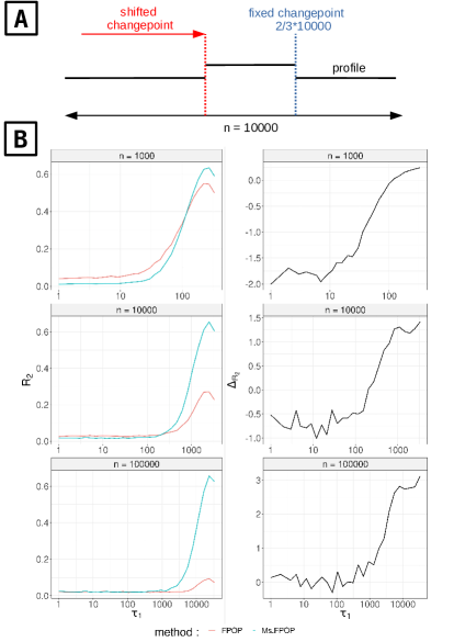
Figure 4: Ms.FPOP increases the probability of finding well spread changepoints on hat simulations. - (A) denoised profile with 2 changepoints. The second changepoint is fixed at $\lfloor\frac{2n}{3}\rfloor$ while the first one ($\tau_{1}$) varies on the interval $[1,\lfloor\frac{n}{3}\rfloor$]. The means of the three resulting segments are set to $\mu_{1}=0$ , $\mu_{2}=\sqrt{\frac{100}{n}}$ and $\mu_{3}=0$ which gives the profile a hat-like appearance. An iid Gaussian noise of mean 0 and variance one is then added (see Design of simulations). - (B) The proportion of replicates for which Ms.FPOP and FPOP return 2 changepoints ($R_{2}$) as well as the $\log_{2}$-ratio of the two estimations ($\Delta_{R_{2}}$) are computed for varying $\tau_{1}$ and $n$.

4.3.2 Extended Range of Simulation Scenarios

Design of Simulations

Following a protocol written by Fearnhead et al. 2020, we simulate different scenarios of iid Gaussian signals. Each scenario is defined by a combination of $D$, $n$, $\tau$, $\mu$. For each scenario we vary the variance $\sigma^{2}$ (see Supplementary Data of [24]). All the simulated profiles, with a variance one, can be seen in H. Based on these initial scenarios we simulate another set of profiles in which profile lengths are multiplied so that each segments contain at least 300 datapoints. These new set of simulated profiles can be seen in G. For each scenario and tested $\sigma^{2}$ we simulate 300 replicates.

Metric

We denote $AE\%$, the average number of times a method is at least as good as other methods in terms of absolute difference between the true number of changes and the estimated number of changes ($\Delta_{D}$), mean squared error (MSE) or adjusted rand index (ARI). The closer to 100 (AE%), the better the method. See Supplementary Data of [24] for a formal definition of this criterion.

Empirical Results

On the simulation of [24] in which a large portion of the segments have a length under 100 the performance of Ms.FPOP are worse than FPOP and MOSUM [25] on almost all scenarios except Dt7 that do not contain any changepoint (see H).

On the second set of profiles, using $\Delta_{D}$ as comparison criterion, we observe on Figure 5 that Ms.FPOP get similar performance or is better than FPOP and MOSUM in all scenarios marginaly to $\sigma^{2}$. The results are similar when we use MSE or ARI as a criterion of comparison (see G).

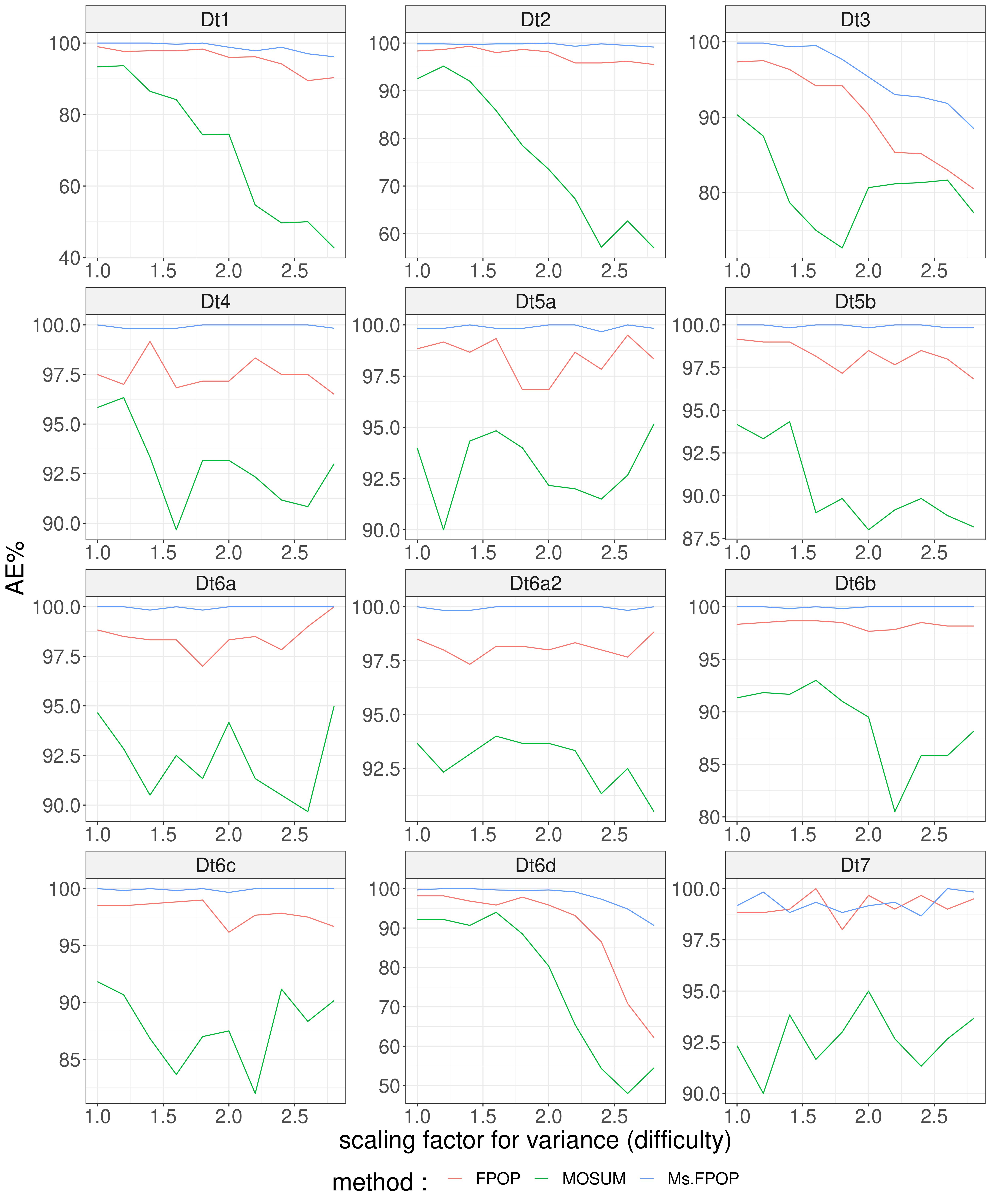
Figure 5: AE% as a function of the scaling factor for the variance (comparison criterion : $\Delta_{D}$). The average number of times a method is at least as good as other methods in terms of $\Delta_{D}$ is computed for FPOP, Ms.FPOP, and MOSUM on different scenarios of iid Gaussian signals and varying $\sigma^{2}$. The smallest segment length is greater or equal to 300 (see Design of Simulations). Each panel stands for the results on one scenario. Corresponding profiles can be viewed in G.

5 Discussion

Extending Functional Pruning Techniques to the Multiscale Penalty

In section 2.2 we have explained how to extend functional pruning techniques to the case of multiscale penalty. In Figures 1 and 3 we have seen that for large signals ($n\geq 10^{5}$) with few changepoints, Ms.FPOP is an order of magnitude faster than Ms.PELT (which relies on inequality based pruning, see A). Even when the number of changepoints increased linearly with the size of the data, Ms.FPOP was still faster than Ms.PELT.

The main update rule 12 of our dynamic programming algorithm suggests to compare each candidate change $s$ with a set of future candidate changes $s^{\prime}$. As we have seen in D, the strategy of randomly drawing one $s^{\prime}$ according to a uniform distribution is the best strategy and allows us to tackle large signals. It is likely that uniform sampling is not optimal. The algorithm alternates between good draws (leading to a strong reduction of $Z_{t,s}$ or even the pruning of $s$) and bad draws (leading to a weak reduction $Z_{t,s}$). On average this is sufficient but improvements are possible. In particular the study of $h(t,s,s^{\prime})=\log(\frac{t-s^{\prime}}{t-s})$ (see Assumption A1), suggests disfavoring $s^{\prime}$ that are too recent or that have been compared recently.

Calibration of $\gamma$ and $\beta$ from the Multiscale Penalty

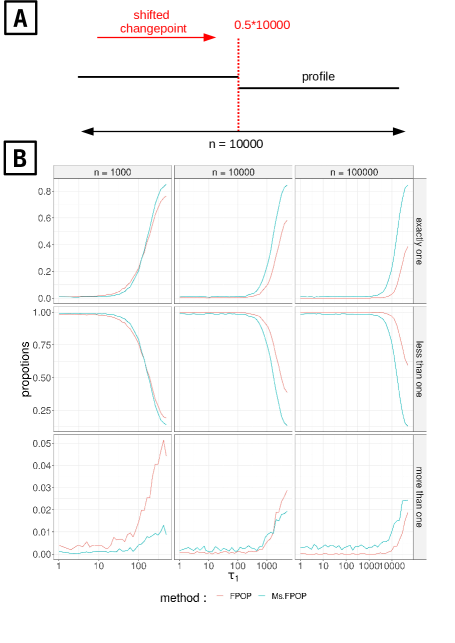
Figure 10: Ms.FPOP increases the probability of finding well spread changepoint on step profiles. - (A) denoised profile with 1 changepoint. The first and unique changepoint ($\tau_{1}$) varies on the interval $[1,\lfloor\frac{n}{2}\rfloor$] (40 positive integers evenly spaced on the $\log$ scale). The difference in mean between the second and the first segment is set to $\sqrt{\frac{70}{n}}$. An iid Gaussian noise of variance one is then added. - (B) The proportion of replicates on which Ms.FPOP and FPOP return one changepoint, less than one changepoint and more than one changepoints are computed for varying profile lengths ($n\in{10^{3},10^{4},10^{5}}$) and $\tau_{1}$.

The least-squares estimator with multiscale penalty proposed by [17] involves two constants $\gamma$ and $\beta$ that still need to be investigated. Using signals simulated under the null hypothesis (no changepoint) we have seen that it is possible to find a pair of constants $\gamma=9$ and $\beta=2.25$ for which Ms.FPOP controls $R_{>0}$. Under this setting we have shown on hat (see section 4.3.1) and step (see Figure 10) simulations that Ms.FPOP is more powerful than FPOP on segmentations with well-spread changepoints. This difference of power grows with $n$. For segmentation with small segments FPOP is more powerful Ms.FPOP when $n$ is small ($\approx 10^{3}$), but for larger $n$ ($\geq 10^{4}$) this difference disappears.

We also tested Ms.FPOP on the benchmark proposed in [24]. The performances of Ms.FPOP are not so good on the original benchmark containing mostly small profiles with small segments but much better for an extended benchmark with larger profiles (see section 4.3.2).

Without additional work on the calibration of the constants, we would thus recommend using Ms.FPOPfor large profiles ($\geq 10^{4}$).

Unknown Variance

All our simulations have been done on signals with known variance, $\sigma^{2}$. However, in real-world situations, this may not always be the case. One approach is to estimate $\sigma^{2}$ and then plugging-in it in the problem, i.e scaling the signal or the penalty by $\frac{1}{\sigma^{2}}$ or $\sigma^{2}$, respectively. A robust estimate of $\sigma^{2}$ can be obtained by calculating the variance of $\Delta_{Y}=Y_{i+1}-Y_{i}$ using either the median absolute deviation or the estimator suggested in [26]. As an alternative, [17] pointed out that one could calibrate the multiplicative constant $L$ of the penalized least-squares estimator using the slope heuristic [27]. Investigating the performances of these various approaches is outside the scope of this paper.

6 Availability of Materials

The scripts used to generate the figures are available in the following GitHub repository: https://github.com/aLiehrmann/MsFPOP_paper . A reference implementation of the Ms.FPOP (and Ms.PELT) algorithm is available in the R package of the same name: https://github.com/aLiehrmann/MsFPOP.

Appendix A PELT for Multiscale Penalized Likelihood

Following the notation of the PELT paper [20] the cost of a segment from $s+1$ to $s^{\prime}$, $s+1:s^{\prime}$ is defined as $\mathcal{C}_{s+1:s^{\prime}}=\sum_{i=s+1}^{s^{\prime}}(y_{i}-\bar{y}_{s+1:s^{\prime}})^{2}-\beta g(s^{\prime}-s).$ In what follow we consider three time points $s<s^{\prime}<t$. Let $\ell=s^{\prime}-s$ denote the length of the sequence of observations between time $s$ and $s^{\prime}$ and $\ell^{\prime}=t-s^{\prime}$ denote the length of the sequence of observations between time $s^{\prime}$ and $t$.

The key condition to apply the PELT algorithm [20] is that up to a constant $K$ adding a changepoints always reduce the cost, that is :

Assumption 2.

$$\mathcal{C}_{s+1:s^{\prime}}+\mathcal{C}_{s^{\prime}+1:t}+K\leq\mathcal{C}_{s+1:t}$$ (18)

The following lemma ensure that such $K$ exists for any $n$ and provide explicit values for $K$ in general and if $g$ is concave.

Lemma 2.

(a) For any function $g$ from $\mathbb{R}$ to $\mathbb{R}$, $\beta\geq 0$, and any $n$, Assumption 2 is true at least for $K=2\beta\min_{1\leq\ell\leq n}\{g(\ell)\}-\beta\max_{1\leq\ell\leq n}\{g(\ell)\}$. (b) If $g$ is concave the condition is true for $K=-\beta g(2)+2\beta g(1).$

Proof.

We first note that

$$m_{n}=\underset{1\leq\ell<n}{\min}\left\{\underset{\begin{subarray}{c}1\leq\ell^{\prime}<n\\ \ell+\ell^{\prime}\leq n\end{subarray}}{\min}\left\{g(\ell)+g(\ell^{\prime})-g(\ell+\ell^{\prime})\right\}\right\}$$

is well defined as the minimum of a finite set. By definition of $m_{n}$ we thus have, for any $1\leq s<s^{\prime}<t\leq n$ and for any $K<\beta m_{n}$, that

$$-\beta g(s^{\prime}-s)-\beta g(t-s^{\prime})+K \leq -\beta g(t-s)$$

Combining this with

$$\sum_{i=s+1}^{s^{\prime}}(y_{i}-\bar{y}_{s+1:s^{\prime}})^{2}+\sum_{i=s^{\prime}+1}^{t}(y_{i}-\bar{y}_{s^{\prime}+1:t})^{2} \leq \sum_{i=s+1}^{t}(y_{i}-\bar{y}_{s+1:t})^{2}.$$

we recover that equation (2) is true for any $K<\beta m_{n}.$

Now for any $\ell$, $\ell^{\prime}$ in $\{1,\ldots,n\}^{2}$ such that $\ell+\ell^{\prime}\leq n$ we have

$$2\min_{1\leq\ell\leq n}\{g(\ell)\}-\max_{1\leq\ell\leq n}\{g(\ell)\}\leq g(\ell)+g(\ell^{\prime})-g(\ell+\ell^{\prime}).$$

Hence we get

$$2\min_{1\leq\ell\leq n}\{g(\ell)\}-\max_{1\leq\ell\leq n}\{g(\ell)\}\leq m_{n},$$

and we recover (a).

In case $g$ is concave using the technical lemma 3 two times we get :

$$\underset{\begin{subarray}{c}1\leq\ell^{\prime}<n\\ \ell+\ell^{\prime}\leq n\end{subarray}}{\min}\left\{g(\ell)+g(\ell^{\prime})-g(\ell+\ell^{\prime})\right\}=g(\ell)+g(1)-g(\ell+1)$$ (19)

and

$$\underset{1\leq\ell<n}{\min}\left\{\underset{\begin{subarray}{c}1\leq\ell^{\prime}<n\\ \ell+\ell^{\prime}\leq n\end{subarray}}{\min}\left\{g(\ell)+g(\ell^{\prime})-g(\ell+\ell^{\prime})\right\}\right\}=2g(1)-g(2)$$

For example, if $g=\log$ we get $K=-\beta\log(2)$ ∎

Lemma 3.

If $g$ is concave then for any $\delta>0$, the function $h:x\rightarrow g(x+\delta)-g(x)$ is non increasing.

Proof.

Consider any $\delta^{\prime}>0$. We have $x+\delta=(1-\alpha)x+\alpha(x+\delta+\delta^{\prime})$ for $\alpha=\delta/(\delta+\delta^{\prime})$ and similarly $x+\delta^{\prime}=(1-\alpha^{\prime})x+\alpha^{\prime}(x+\delta+\delta^{\prime})$ with $\alpha^{\prime}=\delta^{\prime}/(\delta+\delta^{\prime}).$ Using concavity we have

$$g(x+\delta) \geq (1-\alpha)g(x)+\alpha g(x+\delta+\delta^{\prime})$$

$$g(x+\delta^{\prime}) \geq (1-\alpha^{\prime})g(x)+\alpha^{\prime}g(x+\delta+\delta^{\prime}).$$

Suming these two lines and noting that $\alpha+\alpha^{\prime}=1$ we get $g(x+\delta)-g(x)\geq g(x+\delta^{\prime}+\delta)-g(x+\delta^{\prime})$

∎

Appendix B Adaptative PELT for Concave Multiscale Penalty

In the following lemma we show that for our multiscale penalty assuming the function $g$ is concave the constant $K$ in theorme 3.1 of [20] can be chosen adaptively to the length of the last segment.

Lemma 4.

If $g$ is concave and $\beta\geq 0.$ then if at time $s^{\prime}$ we have,

$$F_{s}+\sum_{i=s+1}^{s^{\prime}}(y_{i}-\bar{y}_{s+1:s^{\prime}})^{2}-\beta g(\ell)+K_{s^{\prime}-s=\ell}\geq F_{s^{\prime}},$$

with $K_{\ell}=\beta(g(\ell)+g(1)-g(\ell+1))$ then for any time $t$ larger than $s^{\prime}$ we have :

$$F_{s}+\sum_{i=s+1}^{t}(y_{i}-\bar{y}_{s+1:t})^{2}-\beta g(\ell+\ell^{\prime})\geq F_{s^{\prime}}+\sum_{i=s^{\prime}+1}^{t}(y_{i}-\bar{y}_{s^{\prime}+1:t})^{2}-\beta g(\ell^{\prime}),$$

and thus for any time $t\geq s^{\prime}$, a change at $s$ can never be optimal. Taking $g=\log$ we get $K_{\ell}=-\beta\log(\frac{1}{\ell}+1)\leq-\beta\log(2)$.

Proof.

We follows the proof of Theorem 3.1 of [20] using the fact that if $g$ is concave then equation 19 is true. ∎

Appendix C Ms.FPOP : Calibration of Constants $\gamma$ and $\beta$ from The Multiscale Penalty

The following plots were generated to calibrate the constants in the multiscale penalty of [17]. They are generated as explained in section 4.1.

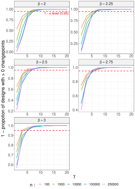
Figure 6: Proportion of stationary Gaussian process replicates on which Ms.FPOP returns at least 1 changepoint ($R_{>0}$). $R_{>0}$ is computed for a series of $\gamma$, $\beta$, and profile lengths (see Design of Simulations in section 4.1).

Appendix D Ms.FPOP Speed Benchmark

Sampling Strategies

We compared the runtime of Ms.FPOP for various sampling strategies (see section 2.2.2). We tested sampling 1, 2, 3 and all future changes. We call these strategies respectively rand 1, rand 2, rand 3 and all. We tested them on the simulation described in section 4.2.

It can be seen on the Figure 7 that sampling 1 future change uniformaly at random is the fastest for all true number of changes and $n=10^{5}.$

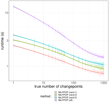
Figure 7: Runtimes as a function of the true number of changepoints. We timed strategies consisting in randomly sampling one, two, three, four or all future candidates on profiles of length $n=10^{5}$ with varying number of true changepoints $D$ (see Design of Simulations in section 4.2) on an Intel Core i7-10810U CPU @ 1.10GHzx12 computer. We observe that, marginaly to $D$, randomly sampling 1 future candidate (Ms.FPOP rand 1) is faster than randomly sampling more than one future candidates, in particular all future candidates.

Larger Profile Lengths $(n=10^{6})$

Figure 8 is obtained as explained in section 4.2, with $n=10^{6}$ and $D\in\{1,500,1000,1500,2000,2500,3000,3500,4000,4500,$
$5000,5500,6000,6500,7000,7500,8000,8500,9000,9500,10000\}$.

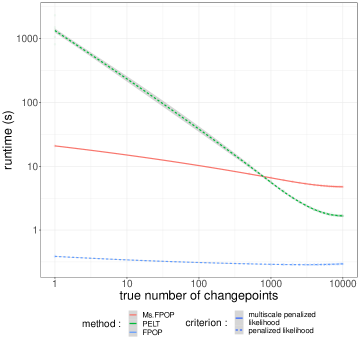
Figure 8: Runtimes as a function of the true number of changepoints. We timed PELT, FPOP, Ms.FPOP on profiles of length $n=10^{6}$ with varying number of true changepoints $D$ (see D) on an Intel Core i7-10810U CPU @ 1.10GHzx12 computer.

Appendix E FPOP vs Ms.FPOP : Simulations on Hat Profiles

Figure 9 is obtained as explained in section 4.3.1.

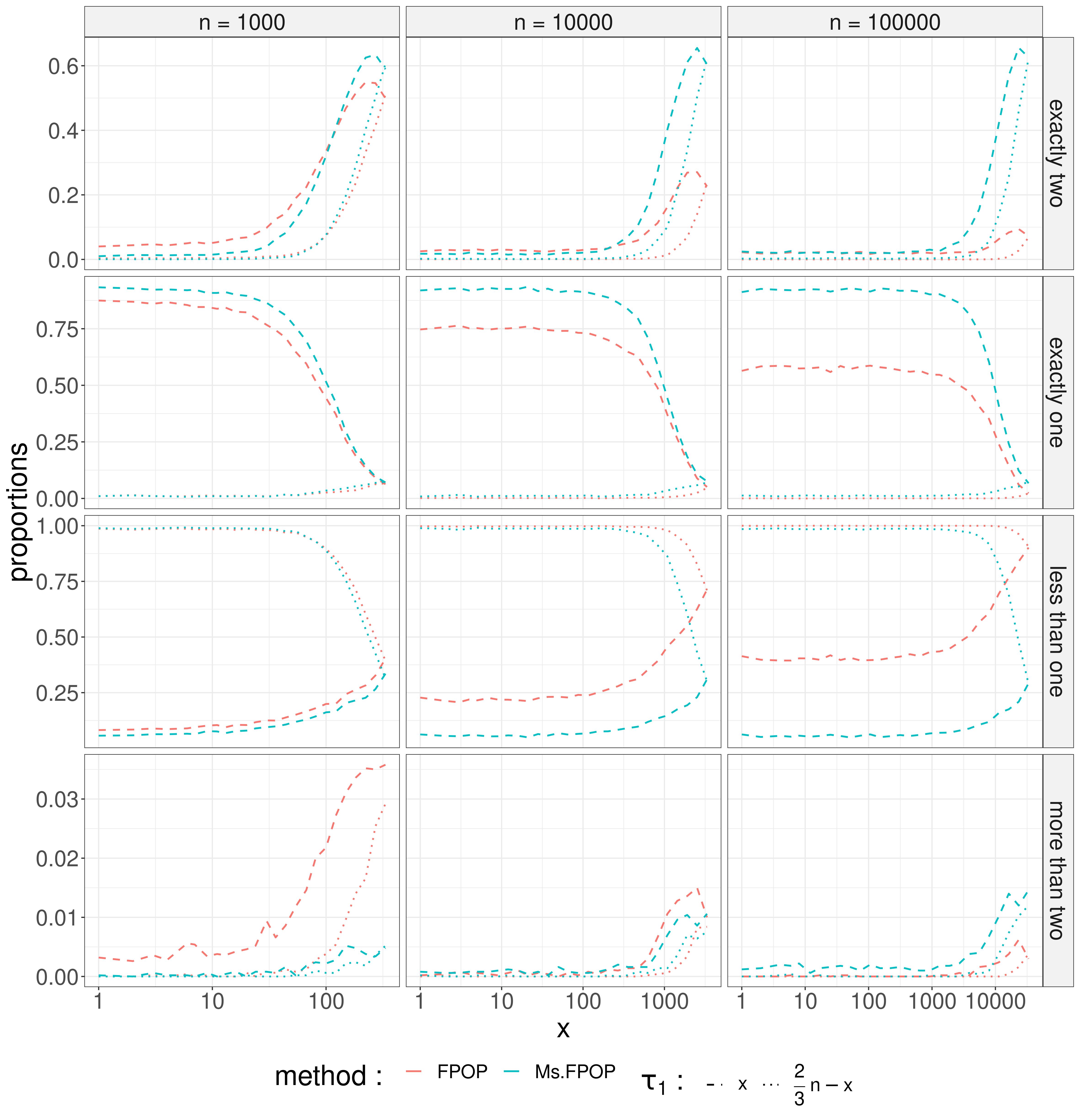
Figure 9: Ms.FPOP increases the probability of finding well spread changepoints on hat profiles. The proportion of replicates for which Ms.FPOP and FPOP return two changepoints, one changepoint, zero changepoint, and more than two changepoints are computed for varying $\tau_{1}\in[1,\lfloor\frac{2}{3}n\rfloor-1]$ and $n\in[10^{3},10^{4},10^{5}]$ on the hat-like profiles (see Design of Simulations in section 4.3.1).

Appendix F FPOP vs Ms.FPOP : Simulations on Step Profiles

Appendix G FPOP vs Ms.FPOP vs MOSUM : Simulations on Several Scenarios of Gaussian Signals (segments length $>300$)

Figures 11, 5, 12, 13 were obtained as explained in section 4.3.2 when considering the benchmark in [24]. On these simulations a large portion of the segments have a length under 100.

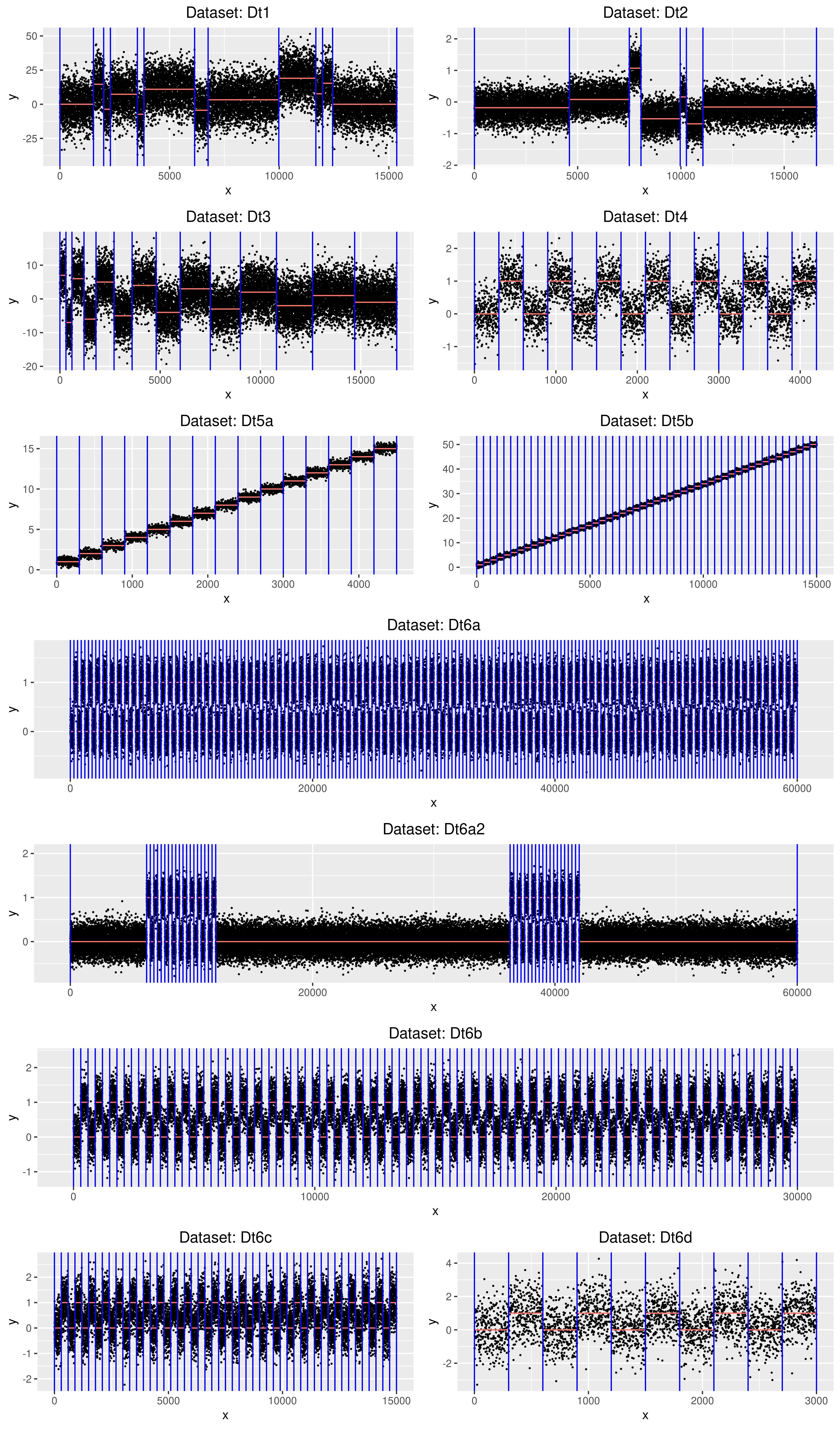
Figure 11: Simulated scenarios of Gaussian signals with minimum segments length equal to 300. All scenarios have been simulated following the protocol written by Fearnhead et al 2020. The length of each segment are scaled so that, in each profile, all segments contain at least 300 datapoints.

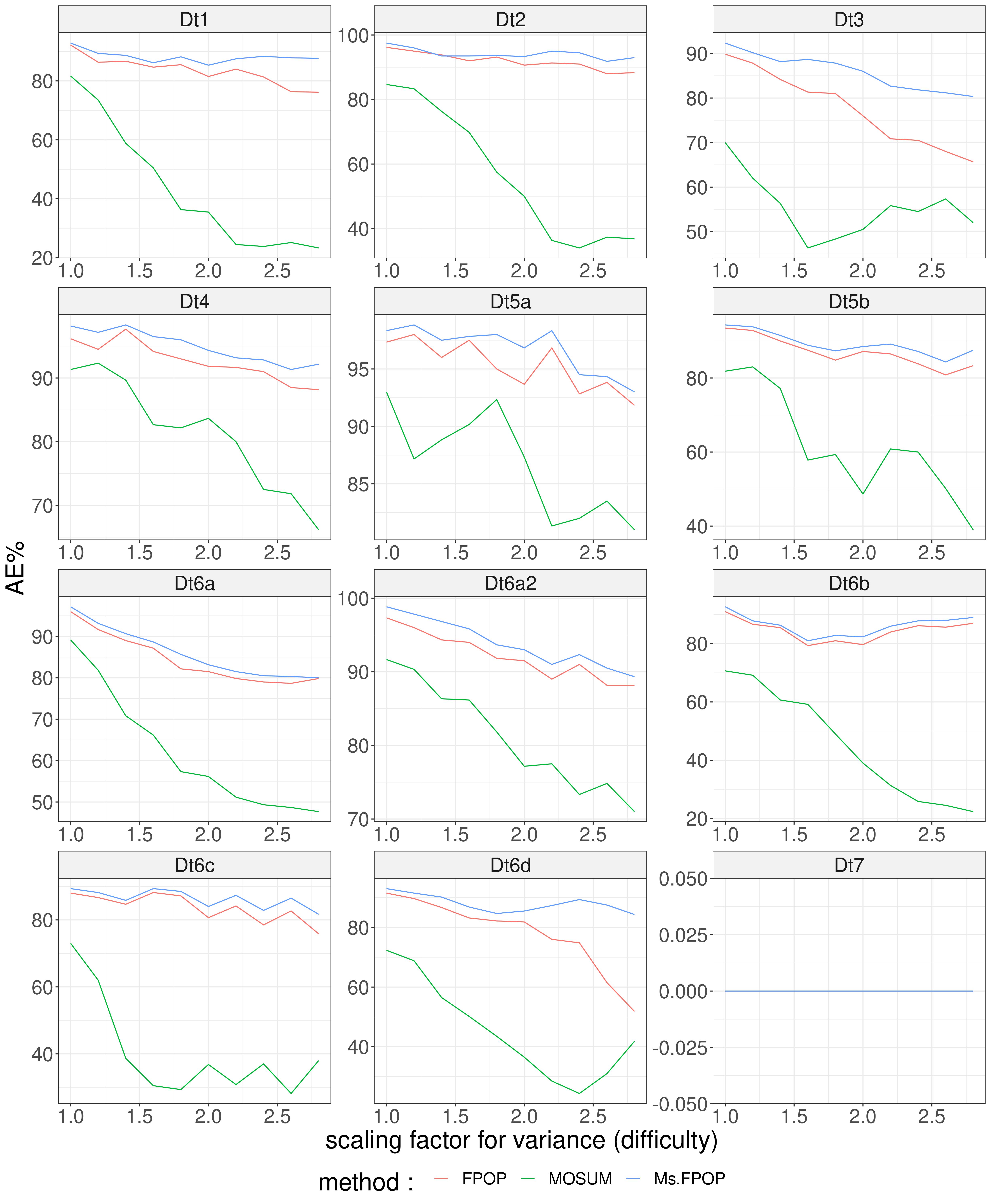
Figure 12: AE% as a function of the scaling factor for the variance (comparison criterion : ARI). The average number of times a method is at least as good as other methods in terms of ARI is computed for FPOP, Ms.FPOP, and MOSUM on different scenarios of iid Gaussian signals and varying $\sigma^{2}$. The smallest segment length is greater or equal to 300 (see Design of Simulations). Each panel stands for the results on one scenario. Corresponding profiles can be viewed in G.

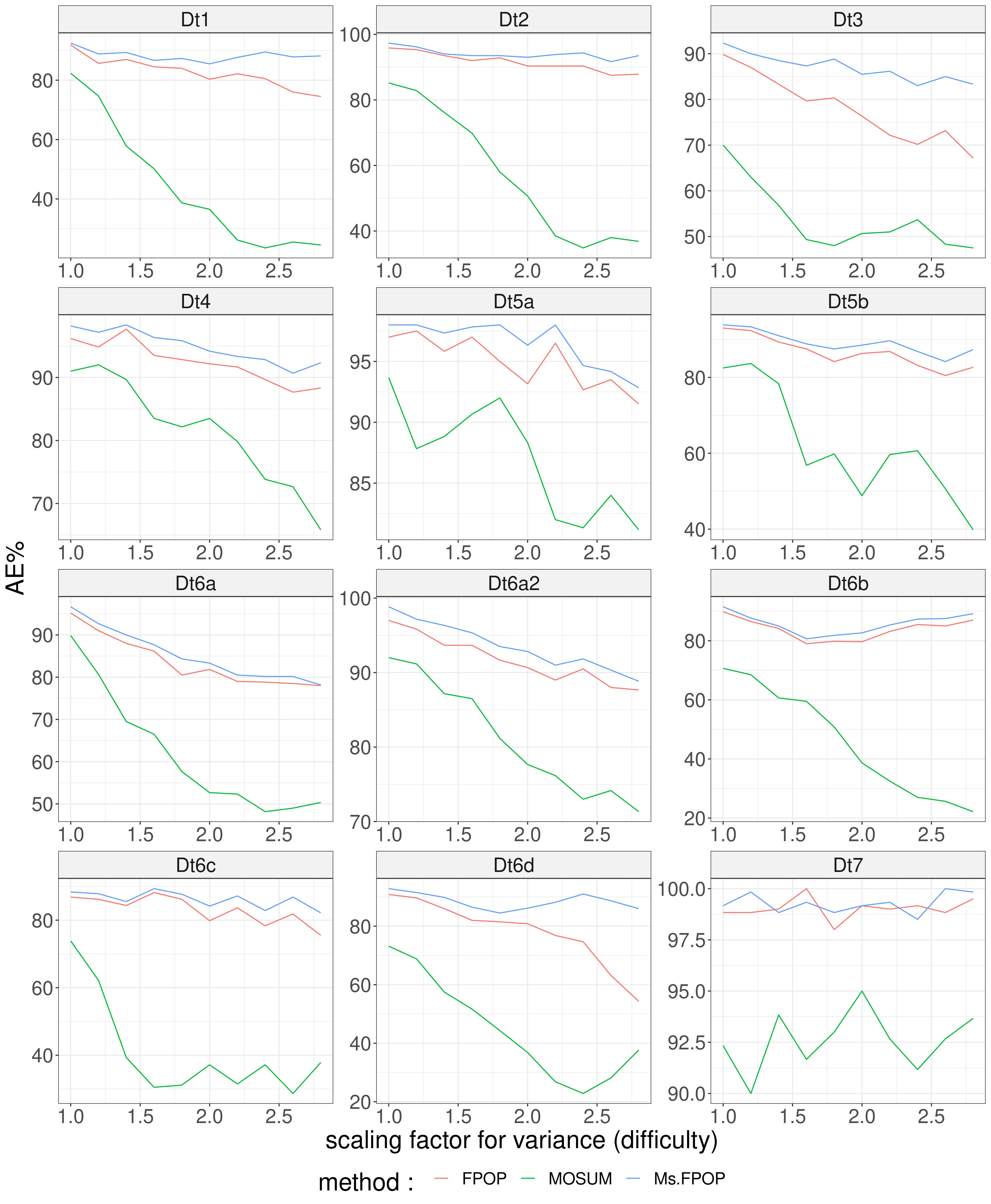
Figure 13: AE% as a function of the scaling factor for the variance (comparison criterion : MSE). The average number of times a method is at least as good as other methods in terms of MSE is computed for FPOP, Ms.FPOP, and MOSUM on different scenarios of iid Gaussian signals and varying $\sigma^{2}$. The smallest segment length is greater or equal to 300 (see Design of Simulations). Each panel stands for the results on one scenario. Corresponding profiles can be viewed in G.

Appendix H FPOP vs Ms.FPOP vs MOSUM : Simulations on Several Scenarios of Gaussian Signals

Figures 14, 15, 16, 17 were obtained as explained in section 4.3.2 when considering an extension of the benchmark in [24]. Based on the initial scenarios we simulated another set of profiles in which segments length are multiplied so that each of segments contain at least 300 datapoints.

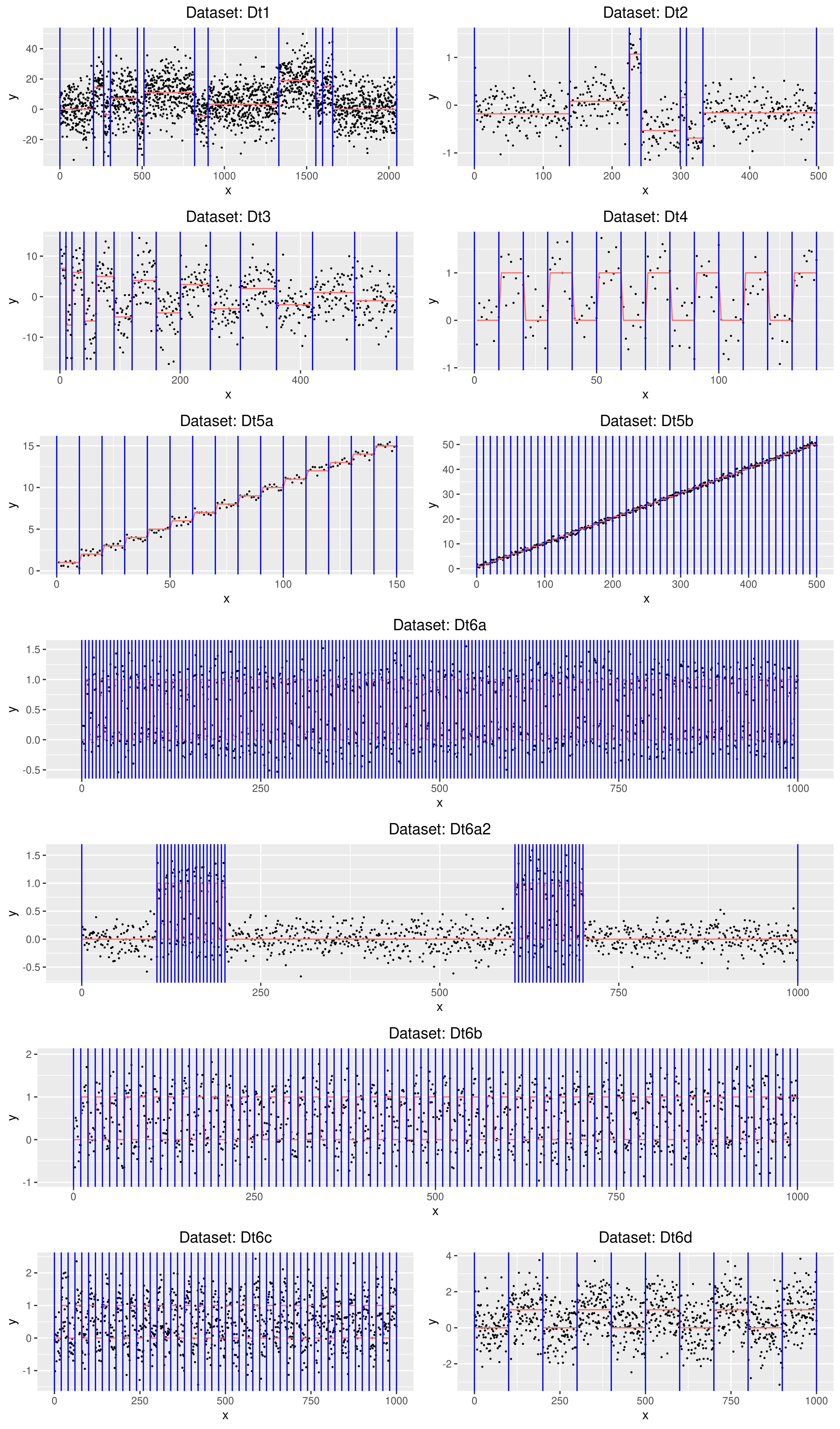
Figure 14: Simulated scenarios of Gaussian signals. All scenarios have been simulated following the protocol written by Fearnhead et al 2020.

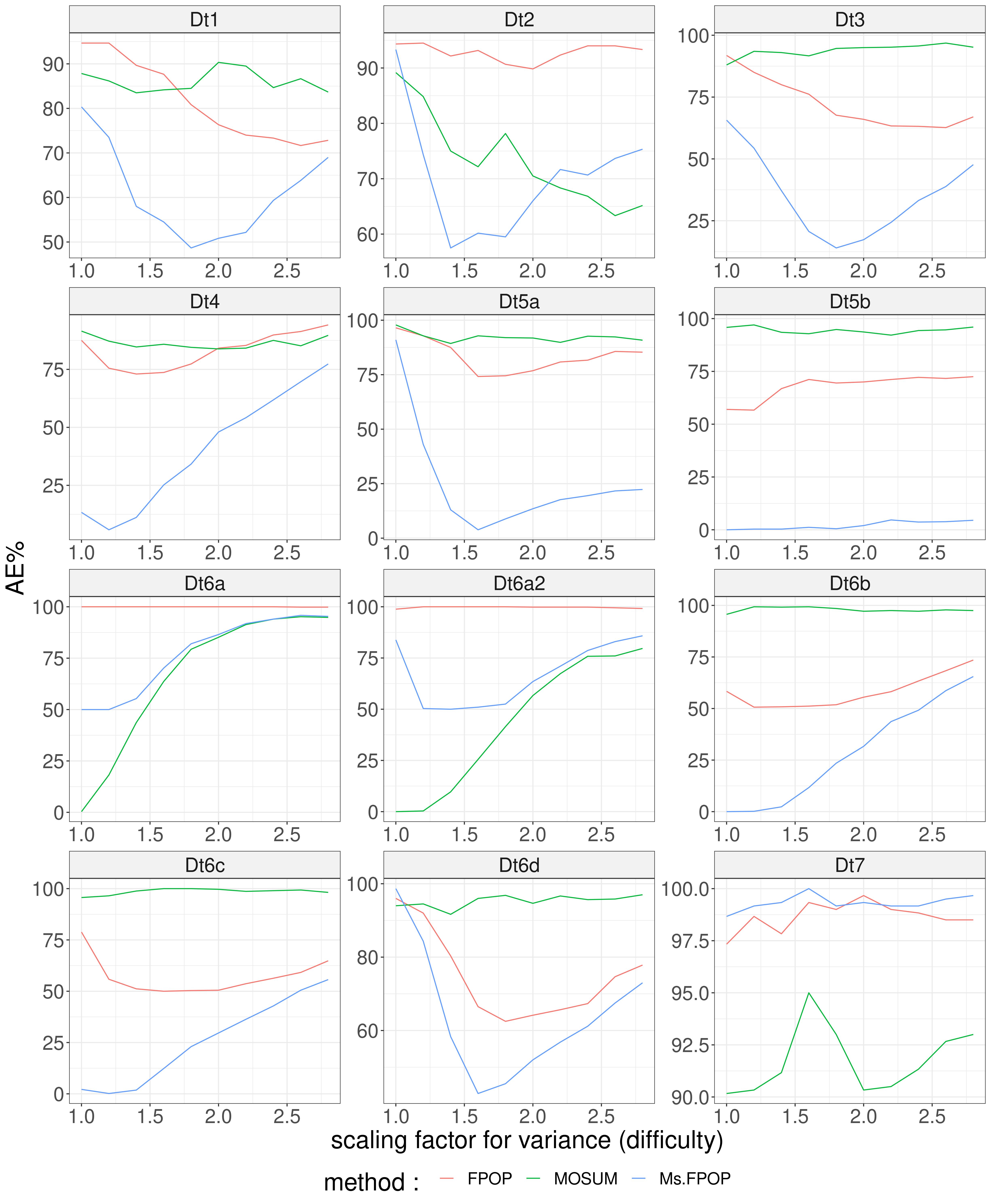
Figure 15: AE% as a function of the scaling factor for the variance (comparison criterion : $\Delta_{D}$). The average number of times a method is at least as good as other methods in terms of $\Delta_{D}$ is computed for FPOP, Ms.FPOP, and MOSUM on different scenarios of iid Gaussian signals and varying $\sigma^{2}$. (see Design of Simulations). Each panel stands for the results on one scenario. Corresponding profiles can be viewed in H.

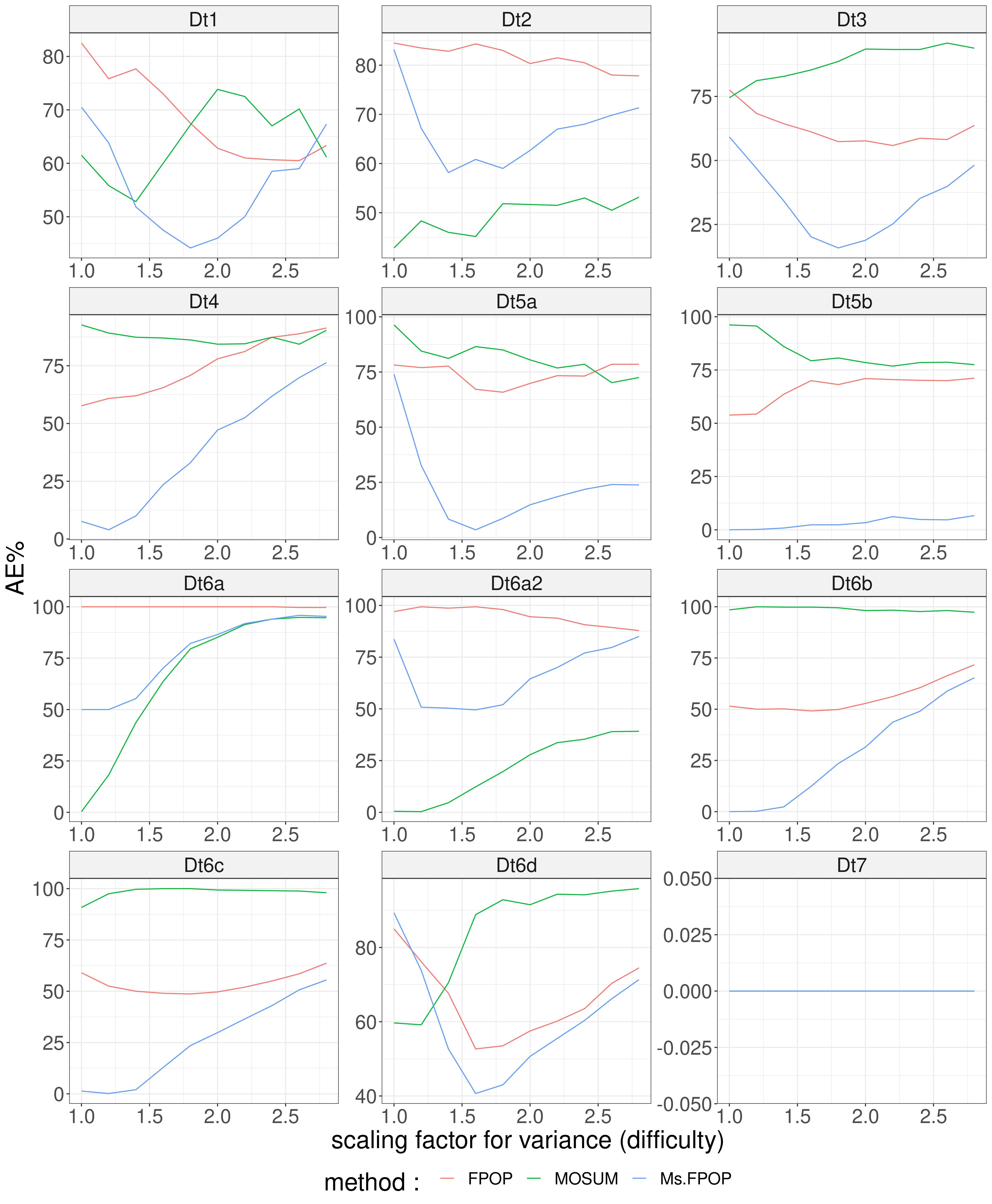
Figure 16: AE% as a function of the scaling factor for the variance (comparison criterion : ARI). The average number of times a method is at least as good as other methods in terms of ARI is computed for FPOP, Ms.FPOP, and MOSUM on different scenarios of iid Gaussian signals and varying $\sigma^{2}$. (see Design of Simulations). Each panel stands for the results on one scenario. Corresponding profiles can be viewed in H.

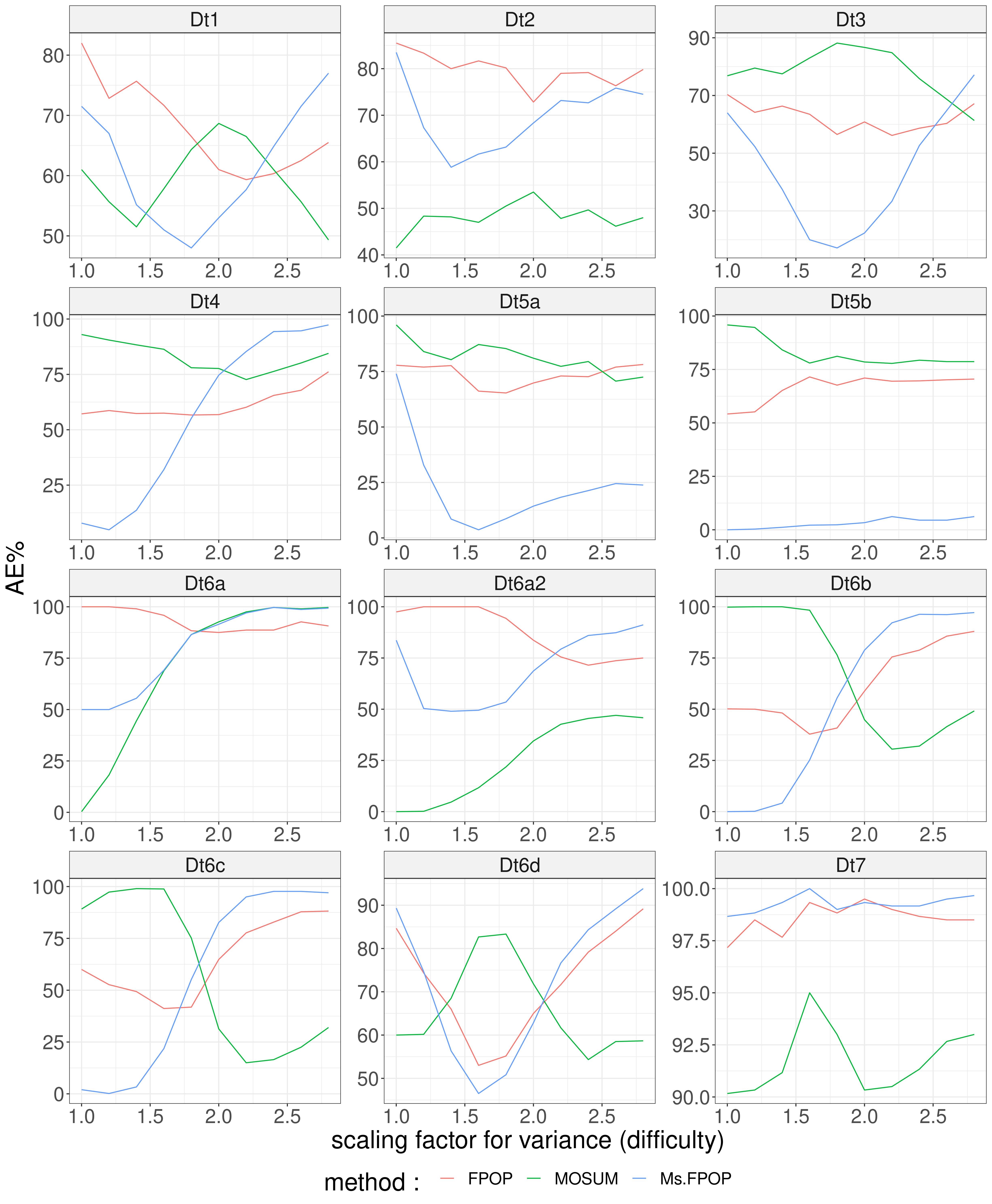
Figure 17: AE% as a function of the scaling factor for the variance (comparison criterion : MSE). The average number of times a method is at least as good as other methods in terms of MSE is computed for FPOP, Ms.FPOP, and MOSUM on different scenarios of iid Gaussian signals and varying $\sigma^{2}$. (see Design of Simulations). Each panel stands for the results on one scenario. Corresponding profiles can be viewed in H.

References

- [1] N. R. Council, et al., Frontiers in massive data analysis, National Academies Press, 2013.
- [2] A. B. Olshen, E. S. Venkatraman, R. Lucito, M. Wigler, Circular binary segmentation for the analysis of array-based dna copy number data, Biostatistics 5 (4) (2004) 557–572.
- [3] F. Picard, S. Robin, M. Lavielle, C. Vaisse, J.-J. Daudin, BMC Bioinformatics 6 (1) (2005) 27.
- [4] J. Bai, P. Perron, Computation and analysis of multiple structural change models, Journal of applied econometrics 18 (1) (2003) 1–22.
- [5] S. Thies, P. Molnár, Bayesian change point analysis of bitcoin returns, Finance Research Letters 27 (2018) 223–227.
- [6] J. Reeves, J. Chen, X. L. Wang, R. Lund, Q. Q. Lu, A review and comparison of changepoint detection techniques for climate data, Journal of Applied Meteorology and Climatology 46 (6) (2007) 900–915.
- [7] E. Galceran, A. G. Cunningham, R. M. Eustice, E. Olson, Multipolicy decision-making for autonomous driving via changepoint-based behavior prediction: Theory and experiment, Autonomous Robots 41 (6) (2017) 1367–1382.
- [8] A. Ranganathan, Pliss: labeling places using online changepoint detection, Autonomous Robots 32 (4) (2012) 351–368.
- [9] S. W. Jewell, T. D. Hocking, P. Fearnhead, D. M. Witten, Fast nonconvex deconvolution of calcium imaging data, Biostatistics 21 (4) (2020) 709–726.
- [10] Y.-C. Y. et al., Least-squares estimation of a step function., Indian Journal of Statistics. 51 (1989) 370–81.
- [11] Émilie Lebarbier, Detecting multiple change-points in the mean of a gaussian process by model selection., Signal Proces. 87 (2005) 717–36.
- [12] Z. Harchaoui, C. Lévy-Leduc, Multiple change-point estimation with a total variation penalty, Journal of the American Statistical Association 105 (492) (2010) 1480–1493.
- [13] K. F. et al., Multiscale change point inference., Royal Statistical Society. 76 (2014) 495–580.
- [14] P. Fryzlewicz, Detecting possibly frequent change-points: Wild binary segmentation 2 and steepest-drop model selection, Journal of the Korean Statistical Society 49 (4) (2020) 1027–1070.
- [15] S. Aminikhanghahi, D. J. Cook, A survey of methods for time series change point detection, Knowledge and information systems 51 (2) (2017) 339–367.
- [16] C. Truong, L. Oudre, N. Vayatis, Selective review of offline change point detection methods, Signal Processing 167 (2020) 107299.
- [17] N. Verzelen, M. Fromont, M. Lerasle, P. Reynaud-Bouret, Optimal change-point detection and localization, arXiv preprint arXiv:2010.11470 (2020).
- [18] G. R. et al., A pruned dynamic programming algorithm to recover the best segmentations with 1 to kmax change-points., Brief Bioinform. 156 (2010) 180–205.
- [19] R. M. et al., On optimal multiple changepoint algorithms for large data., Statistics and Computing. 27 (2017) 519–33.
- [20] R. K. et al., Optimal detection of changepoints with a linear computational cost., Statistics and Computing. 107 (2012) 1590–98.
- [21] B. J. et al., An algorithm for optimal partitioning of data on an interval., IEEE Signal Processing Letters. 12 (2005) 105–8.
- [22] A. et al.., Algorithms for the optimal identification of segment neighborhoods., Bull Math Biol. 51 (1989) 39–54.
- [23] R. Bellman, On the approximation of curves by line segments using dynamic programming., Communications of the ACM. 4 (1961) 284.
- [24] P. Fearnhead, G. Rigaill, Relating and comparing methods for detecting changes in mean, Stat 9 (1) (Jan. 2020).
- [25] A. Meier, C. Kirch, H. Cho, mosum: A package for moving sums in change-point analysis, Journal of Statistical Software 97 (2021) 1–42.
- [26] P. Hall, J. Kay, D. Titterington, Asymptotically optimal difference-based estimation of variance in nonparametric regression, Biometrika 77 (3) (1990) 521–528.
- [27] S. Arlot, Minimal penalties and the slope heuristics: a survey (2019).