Dually Enhanced Propensity Score Estimation in Sequential Recommendation

Abstract.

Sequential recommender systems train their models based on a large amount of implicit user feedback data and may be subject to biases when users are systematically under/over-exposed to certain items. Unbiased learning based on inverse propensity scores (IPS), which estimate the probability of observing a user-item pair given the historical information, has been proposed to address the issue. In these methods, propensity score estimation is usually limited to the view of item, that is, treating the feedback data as sequences of items that interacted with the users. However, the feedback data can also be treated from the view of user, as the sequences of users that interact with the items. Moreover, the two views can jointly enhance the propensity score estimation. Inspired by the observation, we propose to estimate the propensity scores from the views of user and item, called Dually Enhanced Propensity Score Estimation (DEPS). Specifically, given a target user-item pair and the corresponding item and user interaction sequences, DEPS firstly constructs a time-aware causal graph to represent the user-item observational probability. According to the graph, two complementary propensity scores are estimated from the views of item and user, respectively, based on the same set of user feedback data. Finally, two transformers are designed to make the final preference prediction. Theoretical analysis showed the unbiasedness and variance of DEPS. Experimental results on three publicly available and an industrial datasets demonstrated that DEPS can significantly outperform the state-of-the-art baselines.

1. Introduction

Sequential recommendation (Sun et al., 2019; Tan et al., 2016; Liu et al., 2018) has attracted increasing attention from both industry and academic communities. Basically, the key advantage of sequential recommender models lies in the explicit modeling of item chronological correlations. To capture such information accurately, recent years have witnessed lots of efforts based on either Markov chains or recurrent neural networks. While these models have achieved remarkable successes, the observed item correlations can be skewed due to the exposure or selection bias (Chen et al., 2020a). As exampled in Figure 1(a), given a user behavior sequence, the observed next item is a coffeepot cleaner. By building models based on the observational data, one can learn the correlations between cleaner and coffeepot. However, from the user preference perspective, the next item can also be the ink-boxes. But the model has no opportunities to capture the correlations between printer and ink-box because they are not recommended and observed in the data. The bias makes the recommendation less effective, especially when testing environment is more related with the office products.

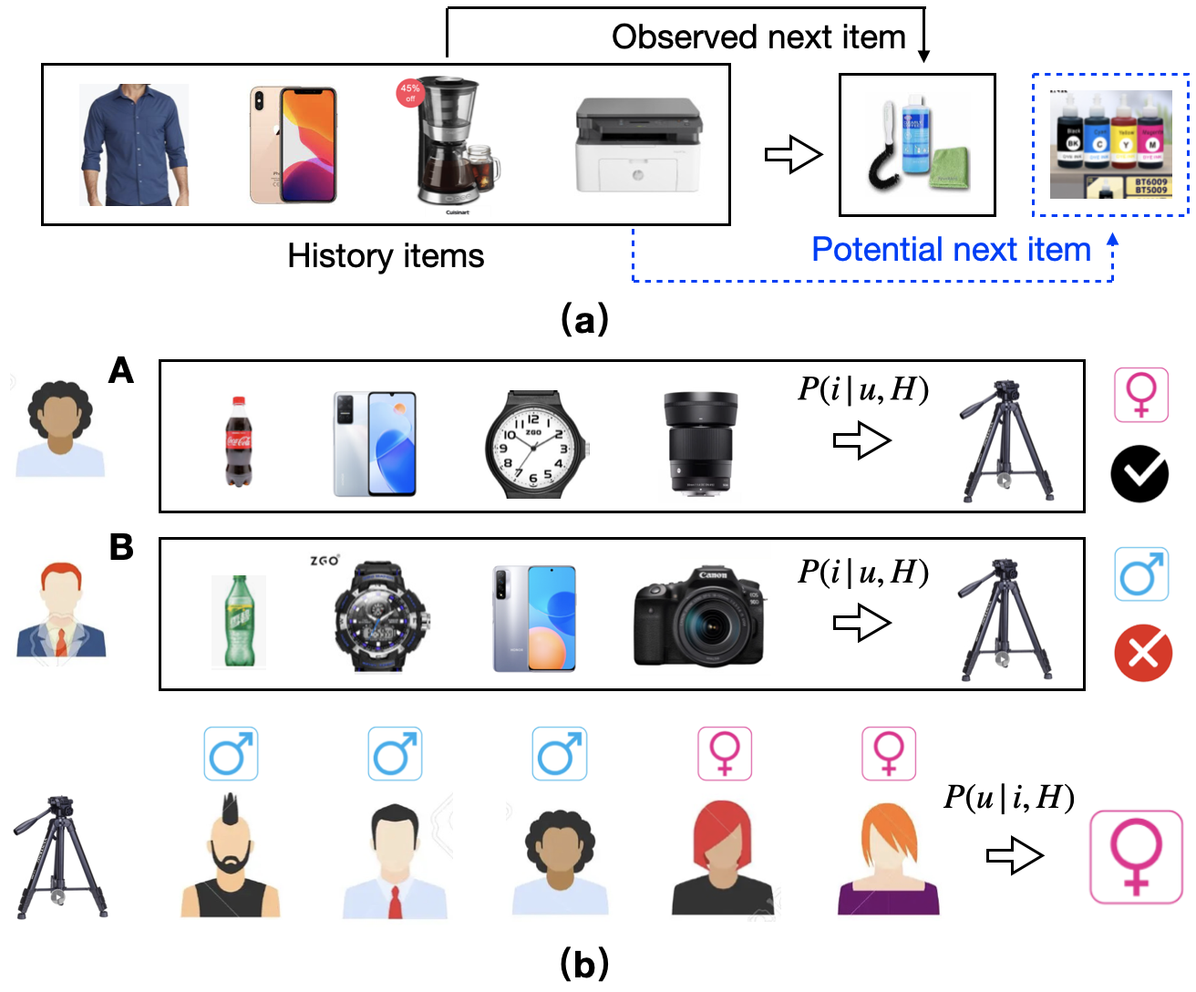
Figure 1. (a) Motivating example of unbiased sequential recommendation. (b) A toy example on the complementary roles of the user prediction problem for existing IPS methods.

In order to alleviate the above problem, previous models are mostly based on the technique of inverse propensity score (IPS) (Schnabel et al., 2016), where if a training sample is more likely to appear in the dataset, then it should have lower weight in the optimization process. In this research line, the key is to accurately approximate the probability of observing a user-item pair $(u,i)$ given the historical information $H$, i.e., $P(u,i|H)$. To this end, previous methods usually decompose $P(u,i|H)$ as $P(i|u,H)P(u|H)$, and focus on parameterizing $P(i|u,H)$ (i.e., estimating $P(u,i|H)$ from view of item (Wang et al., 2022)) to predict which item the user will interact in the next given the previous items. One reason is that estimating propensity scores from the view of item matches well with the online process of sequential recommendation: the users come to the system randomly and the system aims to provide the recommended items immediately.

While these methods are effective, we argue that the probability of observing a user-item pair can also be considered from a dual perspective, that is, for an item, predicting the next interaction user given the ones who have previously interacted with it. In principle, this is equal to decomposing $P(u,i|H)$ in another manner by $P(u|i,H)P(i|H)$, where $P(u|i,H)$ exactly aims to predict the user given an item and the history users (i.e. estimating $P(u,i|H)$ from view of user). Intuitively, for the same item, if two users interact with it for a short time, they should share some similarities at that time. As a result, the previous users may provide useful signals (Fan et al., 2021b) for predicting the next user and the observation of the user-item pair. We believe such a user-oriented method can provide complementary information to the previous item-oriented models.

For example, in Figure 1(b), from the item prediction perspective, the tripod can be observed as the next item for both sequences A and B, since the historical information is similar. However, from the user prediction perspective, we may infer that sequence A should be more likely to be observed, since recently, the tripod is more frequently interacted with by female users, for example, due to the reasons like the promotion sales for the Women’s Day. This example suggests that the temporal user correlation signals may well compensate for traditional item-oriented IPS methods, which should be taken seriously for debiasing sequential recommender.

This paper proposes to build an unbiased sequential recommender model with dually enhanced IPS estimation (called DEPS). The major challenges lie in three aspects: To begin with, the item- and user-oriented IPS are useful, how do we estimate them from the same set of the user feedback data? Secondly, how to combine them is still not clear, especially, since we have to consider the chronological information. At last, how to theoretically ensure that the proposed objective is still unbiased also needs our careful design.

To solve these challenges, we use two GRUs to estimate the propensity scores, one from the view of item and another from the view of user. Also, to make our model DEPS practical, two transformers are used to make the final recommendation, one encodes the historical interacted item sequence of the target user, and the other encodes the user sequence that interacted with the target item. The encoded sequences’ embeddings, as well as the target item and user embeddings, are jointly used to predict the final recommendation score. Moreover, a two-stage learning procedure is designed to estimate the parameters from the modules of propensity score estimation and the item recommendation.

Major contributions of this paper can be concluded as follows:

(1) We highlighted the importance of propensity score estimation from two views and proposed a dually enhanced IPS method for debiasing sequential recommender models.

(2) To achieve the above idea, we implement a double GRU architecture to consider both user- and item-oriented IPS estimation, and theoretically proof the unbiasedness of our objective.

(3) We conduct extensive experiments to demonstrate the effectiveness of our model by comparing it with the state-of-the-art methods based on three publicly available benchmarks and an industrial-scale commercial dataset.

2. Related Work

A lot of research efforts have been made to develop models for sequential recommendation (Sun et al., 2019; Zhou et al., 2018; Chen et al., 2019b; Zhou et al., 2019; Tan et al., 2016; Liu et al., 2018; Fan et al., 2021a). Compared to traditional recommendation (Xue et al., 2017; Rendle et al., 2012), sequential recommendation tries to capture the item chronological correlations. Models based on either Markov chains or recurrent neural networks have been proposed. For example, GRU4Rec+ (Tan et al., 2016) introduces an RNN to encode the historical item sequences as the user preference. BERT4Rec (Sun et al., 2019) proposes an attention-based way (Parikh et al., 2016) to model user behavior sequences practically. BST (Chen et al., 2019b) utilizes the transformer (Parikh et al., 2016) to capture the user preference from the interaction sequences. LightSANs (Fan et al., 2021a) introduce a low-rank decomposed self-attention to the model context of the item. As for model training, S3-Rec (Zhou et al., 2020) incorporates self-supervised and adapts the Pre-train/fine-tune paradigm.

Modern recommender systems have to face variant biases, including selection bias (Marlin et al., 2012), position bias (Zheng et al., 2020; Collins et al., 2018), popularity bias (Zhang et al., 2021a), and exposure bias (Liu et al., 2020; Saito et al., 2020a; Chen et al., 2019a; Chen et al., 2020b; Abdollahpouri and Mansoury, 2020). Biases usually happen on multi sides (Abdollahpouri and Mansoury, 2020; Chen et al., 2020a). For example, item exposure is affected by both the user’s previous behaviors (Liu et al., 2020; Saito et al., 2020a) and the user’s background (Chen et al., 2018, 2019a; Chen et al., 2020b). Wang et al. (2021); Zhang et al. (2021b); Wang et al. (2022) pointed out that sequential scenarios are different and more studies are needed.

One common way to remedy the bias is through inverse propensity score (IPS) (Schnabel et al., 2016). Hu et al. (2008); Devooght et al. (2015) used the prior experience as propensity score to uniformly re-weight the samples. UIR (Saito et al., 2020a) and UBPR (Saito, 2020b) propose to utilize the latent probabilistic model to estimate propensity score. Agarwal et al. (2019); Fang et al. (2019) utilized the intervention harvesting to learn the propensity. Qin et al. (2020); Joachims et al. (2017) learns propensity model with EM algorithms.USR (Wang et al., 2022) proposed a network to estimate propensity scores from the view of item in the sequential recommendation. (Chen et al., 2018, 2019a) pointed out that it is useful to carefully consider the user’s perspective when estimating propensity.

3. Problem Formulation

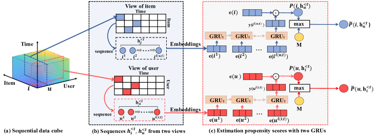
Figure 2. Propensity score estimation in sequential recommendation. (a) Representing historical user-item interactions as a data cube, where item and user can be placed on the axis in any order; (b) Construction of two interaction sequences correspond to a target tuple $(u,i,t)$, from the views of item and user, respectively; (c) Using two GRUs to estimate the propensity scores.

3.1. Sequential Recommendation

Suppose that a sequential recommender system manages a set of user-item historical interactions $\mathcal{D}=\{(u,i,c_{t})\}$ were each tuple $(u,i,c_{t})$ records that at time stamp $t$, a user $u\in\mathcal{U}$ accessed the system and interacted with an item $i\in\mathcal{I}$, and the user’s feedback is $c_{t}\in\{0,1\}$, where $\mathcal{U}$ and $\mathcal{I}$ respectively denote the set of users and items in the system, and $c_{t}=1$ means that the user $u$ clicked the item $i$ and 0 otherwise at time $t$. Moreover, the context information of $(u,i)$ (e.g. user profile and item attribute) collected from the system is often represented as real-valued vectors (embeddings) $\mathbf{e}(u),\mathbf{e}(i)\in\mathbb{R}^{d}$, where $d$ denotes the dimensions of the embeddings.

At a specific time $t$ and given a target user-item pair $(u,i)$, two types interaction sequences can be derived from $\mathcal{D}$: (1) the sequence of items that the user $u$ previously interacted before time $t$: $\mathbf{h}^{<t}_{u}=[i^{1},i^{2},\cdots,i^{l(u,t)}]$, where $l(u,t)$ denotes the number of items the user $u$ interacted before time $t$; (2) the sequence of the users that item $i$ was previously interacted with before time $t$: $\mathbf{h}^{<t}_{i}=[u^{1},u^{2},\cdots,u^{l(i,t)}]$, where $l(i,t)$ denotes the number of users the item $i$ was interacted before time $t$.

Figure 2 (a,b) illustrate that $\mathbf{h}^{<t}_{u}$ and $\mathbf{h}^{<t}_{i}$ are actually dual views of the data cube derived from $\mathcal{D}$. Specifically, by considering the user, item, and time as three axes, $\mathcal{D}$ can be represented as a sparse data cube where the $(u,i,t)$-th element is 1 if $u$ clicked $i$ at time $t$, 0 if observed but not clicked, and NULL if not-interacted. It is obvious that $\mathbf{h}^{<t}_{i}$ and $\mathbf{h}^{<t}_{u}$ are two views of the data cube: (1) view of item: given a user $u$, her/his historical interactions before $t$ are stored in the matrix sliced by $u$. Since $u$ can only interact with one item at a time, we can remove the non-clicked items, sort the remaining items according to the time, and achieve the list $\mathbf{h}^{<t}_{u}$, where $l(u,t)$ is the number of nonzero elements in the sliced matrix; (2) view of user: given an item $i$ and its interaction history, the matrix sliced by $i$ can also be aggregated into another list $\mathbf{h}^{<t}_{i}$.

The task of sequential recommendation becomes, based on the user-item interactions and users’ feedback in $\mathcal{D}$, learning a function $\hat{r}_{t}=f(u,i,\mathbf{h}_{u}^{<t},\mathbf{h}_{i}^{<t})$ that predicts user $u$’s preference on item $i$ at time $t$. It is expected that the predicted preference is close the true while un-observable user preference $r_{t}\in\{0,1\}$ at time $t$, where $r_{t}=1$ means that $i$ is preferred by $u$ at time $t$, and 0 otherwise.

3.2. Biases in Sequential Recommendation

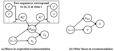
Figure 3. Causal graphs of bias in (sequential) recommendation.

In sequential recommendation, bias happens when the user $u$ is systematically under/over-exposed to certain items. As shown in Figure 3(a) and from a causal sense, a user clicks an item at time $t$ ($c_{t}=1$) only if the item $i$ is relevant to the user $u$ ($r_{t}=1$) and the $i$ is exposed to $u$ ($o_{uit}=1$), where $o_{uit}\in\{0,1\}$ and $r_{t}\in\{0,1\}$ respectively denote whether the user $u$ is aware of item $i$ and is relevant to $i$, or formally $c_{t}=r_{t}\cdot o_{uit}$. Further suppose that the two interaction sequences $\mathbf{h}^{<t}_{u}$ and $\mathbf{h}^{<t}_{i}$ will also influence whether $u$ is aware of the $i$. Since the model predicts the user preference $r_{t}$ with the observed clicks $c_{t}$, the prediction is inevitably biased by the item exposure $o_{uit}$. This is because the $o_{uit}$ becomes a confounder after observing the click in the causal graph (i.e., click as a collider (Pearl, 2009)).

Formally, the probability of a user $u$ clicks an item $i$ at time $t$ can be factorized as the probability that $i$ is observable to the user (i.e., $o_{uit}=1$) and the probability that $(u,i)$ is relevant $r_{t}=1$:

(1) $$P(c_{t}=1|u,i,t)=P(r_{t}=1|u,i,\mathbf{h}^{<t}_{u},\mathbf{h}^{<t}_{i})\cdot P(o_{uit}=1).$$

As have shown in Figure 1, existing studies usually estimate $P(o_{uit}=1)$ only from the view of item, ignoring the dual view of user. Also, the estimation need to take the chronological information (i.e., $\mathbf{h}^{<t}_{u}$ and $\mathbf{h}^{<t}_{i}$) into consideration.

3.3. Unbiased Objective for Recommendation

Ideally, the learning objective for recommendation (including the sequential and non-sequential scenarios) should be constructed based on the correlations between the true preference and the predicted score by the recommendation model:

(2) $$\mathcal{L}^{\text{ideal}}_{n}=\sum_{u\in\mathcal{U}}\sum_{i\in\mathcal{I}}\delta(r,\hat{r}(u,i)),$$

where $\hat{r}(u,i)$ is the prediction by the recommendation model, $r$ is the true preference, and $\delta(\cdot,\cdot)$ is the loss function defined over each user-item pair. Note that in non-sequential recommendation, time $t$ and historical information $\mathbf{h}_{u}^{<t},\mathbf{h}_{i}^{<t}$ are not considered. In real world, however, $\mathcal{L}^{\text{ideal}}_{n}$ cannot be directly optimized because the true preference $r$ cannot be observed.

Traditional RS regard the observed clicks $c$ as the labels to learn the models, which is inevitably influenced by the exposure or self-selection bias as shown in Figure 3(b). A practical solution is to remedy the biases through the propensity score of the confounder (Chen et al., 2020a). A typical approach developed under the non-sequential scenarios is utilizing the propensity score $P(o=1)$ to weigh each observed interaction:

(3) $$\mathcal{L}^{\text{unbiased}}_{n}=\sum_{u\in\mathcal{U}}\sum_{i\in\mathcal{I}}\left[\mathbb{I}(o_{ui}=1)\frac{\delta(c,\hat{r}(u,i))}{P(o_{ui}=1)}\right],$$

where $\mathbb{I}(\cdot)$ is the indicator function, and Eq. (3) is an unbiased estimation of the ideal objective Eq. (2), i.e., $\mathbb{E}_{o}\left[\mathcal{L}^{\mathrm{unbiased}}_{n}\right]$ = $\mathcal{L}^{\mathrm{ideal}}_{n}$. Please refer to (Chen et al., 2020a) for more details.

Unbiased recommendation models have been developed under the framework. Generalizing these methods to sequential recommendation is a non-trial task. In this paper, we presented an approach to utilizing the user-item interaction sequences to estimate the propensity scores framework called DEPS.

4. Our Approach: DEPS

In this section, we proposed an unbiased objective for the sequential recommendation. After that, a dually enhanced IPS estimation model called DEPS is developed to estimate the propensity scores in the objective of sequential recommendations. Finally, two transformers are proposed to adapt our framework in a practical way.

4.1. Unbiased Loss for Sequential Recommendation

Given a user-item historical interactions $\mathcal{D}$, we define the ideal learning objective of sequential recommendation as evaluating the preference at each time that the users access the system:

(4) $$\mathcal{L}^{\text{ideal}}_{s}=\sum_{u\in\mathcal{U}}\sum_{t:(u,i^{\prime},c_{t})\in\mathcal{D}}\sum_{i\in\mathcal{I}}\delta(r_{t},\hat{r}_{t}(u,i,\mathbf{h}^{<t}_{i},\mathbf{h}^{<t}_{u})),$$

where $\hat{r}(u,i,\mathbf{h}_{i}^{<t},\mathbf{h}_{u}^{<t})$ is the prediction by the sequential recommendation model, and $r_{t}$ is the true while un-observable preference at time $t$. Different from the non-sequential unbiased recommender models, the propensity score in sequential recommendation is related to the time, as shown in the causal graph in Figure 3(a). One way to achieve the unbiased sequential recommendation learning objective is estimating the propensity score $P(o_{uit}=1)$ corresponds to $(u,i)$ at time $t$, based on the historical interaction sequences of $\mathbf{h}^{<t}_{i}$ and $\mathbf{h}^{<t}_{u}$, as shown in the following theorem.

Theorem 1 (Time-aware Unbiased Learning Objective).

Given user-item interactions $\mathcal{D}=\{(u,i,c_{t})\}$, we have

(5) $$\mathbb{E}_{o}\left[\mathcal{L}^{\mathrm{unbiased}}_{s}\right]=\mathbb{E}_{o}\left[\alpha\mathcal{L}_{u}+(1-\alpha)\mathcal{L}_{i}\right]=\mathcal{L}^{\mathrm{ideal}}_{s},$$

where $\alpha\in[0,1]$ is the co-efficient that balances the two objectives:

$$\mathcal{L}_{u}=\sum_{(u,i,c_{t})\in\mathcal{D}}\left[\frac{\delta(c_{t},\hat{r}_{t})}{P(i,\mathbf{h}^{<t}_{u})}\right]=\sum_{u\in\mathcal{U}}\sum_{(i,c_{t})\in\mathcal{D}^{u}}\frac{\delta(c_{t},\hat{r}_{t})}{P(i,\mathbf{h}^{<t}_{u})},$$

$$\mathcal{L}_{i}=\sum_{(u,i,c_{t})\in\mathcal{D}}\left[\frac{\delta(c_{t},\hat{r}_{t})}{P(u,\mathbf{h}^{<t}_{i})}\right]=\sum_{i\in\mathcal{I}}\sum_{(u,c_{t})\in\mathcal{D}^{i}}\frac{\delta(c_{t},\hat{r}_{t})}{P(u,\mathbf{h}^{<t}_{i})},$$

where $\mathcal{D}^{u}=\{(i,c_{t}):(u,i,c_{t})\in\mathcal{D}\}$, $\mathcal{D}^{i}=\{(u,c_{t}):(u,i,c_{t})\in\mathcal{D}\}$, $P(i,\mathbf{h}^{<t}_{u})$ is the probability that $i$ and $\mathbf{h}^{<t}_{i}$ appear, and $P(u,\mathbf{h}^{<t}_{i})$ is the probability that $u$ and $\mathbf{h}^{<t}_{i}$ appear.

Proof of Theorem 1 can be found in the Appendix A.1. From the theorem, we can see that an unbiased learning objective for sequential recommendation can be achieved either from the view of user $\mathcal{L}_{u}$ or the view of item $\mathcal{L}_{i}$. Moreover, it is easy to know that the average of the two unbiased losses, i.e., $\mathcal{L}_{s}^{\text{unbiased}}$ defined in Eq. (5), is still an unbiased objective.

Considering that the propensity scores play as the denominators in $\mathcal{L}_{i}$ and $\mathcal{L}_{u}$. To enhance the estimation stability, clip technique (Saito et al., 2020b) is applied to the estimated probabilities in Eq. (8) and Eq. (9), achieving

(6) $$\widetilde{P}(i,\mathbf{h}^{<t}_{u})= \max\{P(i,\mathbf{h}^{<t}_{u}),M\},$$

(7) $$\widetilde{P}(u,\mathbf{h}^{<t}_{i})= \max\{P(u,\mathbf{h}^{<t}_{i}),M\},$$

where $M\in(0,1)$ is the clip value. We show that with the clipped propensity scores the estimation variance can be bounded:

Theorem 2 (Estimation Variance).

Let $L_{u}^{t}=\frac{\delta(c_{t},\hat{r}_{t})}{\widetilde{P}(u,\mathbf{h}^{<t}_{i})}$ and $L_{i}^{t}=\frac{\delta(c_{t},\hat{r}_{t})}{\widetilde{P}(i,\mathbf{h}^{<t}_{u})}$ are two random variables w.r.t. loss on a single training sample $(i,u,c_{t})\in\mathcal{D}$, $\alpha L_{u}^{t}+(1-\alpha)L_{i}^{t}$’s estimation variance satisfies:

$$\mathbb{V}\left[\alpha L_{u}^{t}+(1-\alpha)L_{i}^{t}\right]\leq\max\{\mathbb{V}\left[L_{u}^{t}\right],\mathbb{V}\left[L_{i}^{t}\right]\}\leq\left(\frac{1}{M}-1\right)\delta^{2}(r_{t},\hat{r}_{t}).$$

Proof of Theorem 2 can be found in the Appendix A.2. We conclude that the averaged loss would not bring additional variance. Intuitively, the clip value $M$ is a trade-off between the unbiasedness and the variance and provides a mechanism to control the variance. A larger $M$ leads to lower variance and more bias. We show that the clip technique in  Saito et al. (2020b) still works in a dual perspective.

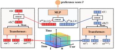
Figure 4. Two transformers based sequential recommender model with sequences from both users and items.

The above analysis provides an elegant and theoretically sound approach to learning an unbiased sequential recommendation model with three steps: (1) for each tuple $(u,i,\mathbf{h}^{<t}_{u},\mathbf{h}^{<t}_{i})$, estimating two propensity scores $\widetilde{P}(i,\mathbf{h}^{<t}_{u})$ and $\widetilde{P}(u,\mathbf{h}^{<t}_{i})$; (2) developing a sequential recommender model, and (3) training the parameters which involves minimizing the averaged loss $\alpha\mathcal{L}_{i}+(1-\alpha)\mathcal{L}_{u}$. Next, we show an implementation of the step (1) with two GRUs in Section 4.2. Secton 4.3 and Section 4.4 respectively implement the step (2) and step (3).

4.2. Estimating Propensity Scores with GRUs

In the real world, sequences $\mathbf{h}^{<t}_{u}$ and $\mathbf{h}^{<t}_{i}$ are very sparse and short compared to the whole sets of items and users. In this paper, we resort to the neural language model of GRU (Cho et al., 2014) for estimating the propensity scores. Also, according to Theorem 2, the clip technique is applied to the estimated propensity scores.

Specifically, two GRUs are respectively used to estimate the $P(i,\mathbf{h}^{<t}_{u})$ and $P(u,\mathbf{h}^{<t}_{i})$, as shown in Figure 2(c). Specifically, given a tuple $(u,i,\mathbf{h}^{<t}_{u},\mathbf{h}^{<t}_{i})$, its propensity score from the view of item is estimated as the maximum value of $M$ and $P(i,\mathbf{h}^{<t}_{u})$, where $P(i,\mathbf{h}^{<t}_{u})$ is proportional to the dot product of $i$’s embedding $\mathbf{e}(i)$, and the output of a GRU which takes the sequence $\mathbf{h}^{<t}_{u}=[i^{1},i^{2},\cdots,i^{l(u,t)}]$ as input. By applying the clip technique in Eq. (6), we write the estimated propensity score from view of item as:

(8) $$\widetilde{P}(i,\mathbf{h}^{<t}_{u})=\max\left\{\frac{\exp{\left(\mathbf{e}(i)^{T}\mathbf{y}(i^{l(u,t)})\right)}}{\sum_{i^{\prime}\in\mathcal{I}}\exp{\left(\mathbf{e}(i^{\prime})^{T}\mathbf{y}(i^{l(u,t)})\right)}},M\right\},$$

where $\mathbf{y}(i^{l(u,t)})\in\mathbb{R}^{d}$ is the GRU output from its last layer (i.e., corresponds to the $l(u,t)$-th input). The GRU scans the items in $\mathbf{h}^{<t}_{u}$ as follows: at the $k$-th ($k=1,\cdots,l(u,t)$) layer, it takes the embedding of the $k$-th item $\mathbf{e}(i^{k})$ as input, and outputs $\mathbf{y}(i^{k})$ which is the representation for the scanned sub-sequence $[i^{1},i^{2},\cdots,i^{k}]$:

$$\mathbf{y}(i^{k}),\mathbf{z}^{k}=\textbf{GRU}_{1}(\mathbf{e}(i^{k}),\mathbf{z}^{k-1}),$$

where $\mathbf{z}^{k}$ and $\mathbf{z}^{k-1}$ are the hidden vectors of $k$-th and $(k-1)$-th steps, and GRU₁ is the GRU cell that processes the sequence from the view of item.

Similarly, given a tuple $(u,i,\mathbf{h}^{<t}_{u},\mathbf{h}^{<t}_{i})$, its propensity score can also be estimated from the view of user: the maximum of $P(u,\mathbf{h}^{<t}_{i})$ and $M$, where $P(u,\mathbf{h}^{<t}_{i})$ is proportional to the dot product of the user embedding $\mathbf{e}(u)$ and the representation of sequence $\mathbf{h}^{<t}_{i}=[u^{1},u^{2},\cdots,u^{l(i,t)}]$. By applying the clip technique in Eq. (7), we write the estimated propensity score from view of user as:

(9) $$\widetilde{P}(u,\mathbf{h}^{<t}_{i})=\max\left\{\frac{\exp{\left(\mathbf{e}(u)^{T}\mathbf{y}(u^{l(i,t)})\right)}}{\sum_{u^{\prime}\in\mathcal{U}}\exp{\left(\mathbf{e}(u^{\prime})^{T}\mathbf{y}(u^{l(i,t)})\right)}},M\right\},$$

where $\mathbf{y}(i^{l(u,t)})\in\mathbb{R}^{d}$ is the output of another GRU which scans $\mathbf{h}^{<t}_{i}$ as follows: at the $k$-th layer, it takes the embedding of the $k$-th user $\mathbf{e}(u^{k})$ as input, and output $\mathbf{y}(u^{k})$ representation for the scanned sub-sequence $[u^{1},u^{2},\cdots,u^{k}]$:

$$\mathbf{y}(u^{k}),\mathbf{z}^{k}=\textbf{GRU}_{2}(\mathbf{e}(u^{k}),\mathbf{z}^{k-1}),$$

where $\mathbf{z}^{k}$ and $\mathbf{z}^{k-1}$ are the hidden vectors, and $\textbf{GRU}_{2}$ is another GRU that processes the interaction sequence from the view of user.

4.3. Backbone: Transformer-based Recommender

As shown Figure 4, the implementation of the sequential recommendation model consists of a Transformer Layer and a Prediction Layer. The Transformer Layer consists of two transformers (Parikh et al., 2016). One converts the sequence $\mathbf{h}_{u}^{<t}$ and the target item $i$ into representation vector, and another converts the sequence $\mathbf{h}_{i}^{<t}$ and the target user $u$ into another representation vector. The Prediction Layer concatenates the vectors and makes the prediction with an MLP.

4.3.1. Transformer Layer

The overall item representation of the input tuple $(u,i,t)$ can be represented as the concat of item id embedding and user historical sequence embeddings:

(10) $$\mathbf{e}^{\textrm{iv}}(u,i,t)=\left[\mathbf{e}(\mathbf{h}^{<t}_{u})\|\mathbf{e}(i)\right],$$

where operator ‘$\|$’ concatenates two vectors, $\mathbf{e}(i)$ is the embedding of the items, $\mathbf{h}^{<t}_{u}=[i^{1},i^{2},\cdots,i^{l(u,t)}]$ is the user sequence related to the target user $u$, and $\mathbf{e}(\mathbf{h}^{<t}_{u})$ is the vector that encodes the sequence, defined as the mean of the vectors outputted by a transformer:

(11) $$\mathbf{e}(\mathbf{h}^{<t}_{u})=\text{Mean}\left(\textbf{Transformer${}_{1}$}\left([\mathbf{e}(i^{1}),\cdots,\mathbf{e}(i^{l(u,t)})]\right)\right),$$

where ‘Mean’ is the mean pooling operation for all the input vectors, and Transformer₁($\cdot$) is a transformer (Parikh et al., 2016) architecture.

Similarly, the overall item representation of the input tuple $(u,i,t)$ can be represented as the concat of user id embedding and item historical sequence embeddings:

(12) $$\mathbf{e}^{\textrm{uv}}(u,i,t)=\left[\mathbf{e}(\mathbf{h}^{<t}_{i})\|\mathbf{e}(u)\right],$$

$\mathbf{e}(u)$ is the embedding of the target user $i$, $\mathbf{h}^{<t}_{i}=[u^{1},u^{2},\cdots,u^{l(i,t)}]$ is item sequence interacted by the target item $i$, and $\mathbf{e}(\mathbf{h}^{<t}_{i})$ is the mean of the output of another transformer:

(13) $$\mathbf{e}(\mathbf{h}^{<t}_{i})=\text{Mean}\left(\textbf{Transformer${}_{2}$}\left([\mathbf{e}(u^{1}),\cdots,\mathbf{e}(u^{l(i,t)})]\right)\right),$$

where Transformer₂($\cdot$) is another transformer architecture.

4.3.2. Prediction Layer

Finally, an Multi-Layer Perception (MLP) is applied which takes $\mathbf{e}^{\textrm{iv}}(u,i,t)$ and $\mathbf{e}^{\textrm{uv}}(u,i,t)$ as inputs, and outputs the predicted preference $\hat{r}$:

(14) $$\hat{r}=\sigma(\textbf{MLP}(\mathbf{e}^{\text{iv}}(u,i,t)||\mathbf{e}^{\text{uv}}(u,i,t))),$$

where ‘$\sigma$’ is the sigmoid function operation and MLP is a two-layer fully connected neural network that takes both $\mathbf{e}^{\text{iv}}(u,i,t)$ and $\mathbf{e}^{\text{uv}}(u,i,t)$ as inputs.

0:  Training set $\mathcal{D}=\{(u,i,c_{t})\}$, iteration numbers $n_{p},n_{u},n_{b}$, coefficients $\lambda_{p}$

0:  $\mathbf{\Theta}=\{\theta_{e},\theta_{p},\theta_{t},\theta_{m}\}$

1:  $\mathbf{\Theta}\leftarrow$ random values

2:  $\mathcal{H}\leftarrow\left\{\mathbf{h}_{u}^{<t}|u\in\mathcal{U}\right\}\cup\left\{\mathbf{h}_{i}^{<t}|i\in\mathcal{I}\right\}${Extract seq. from $\mathcal{D}$}

3:  for $n=1,\cdots,n_{p}$ do

4:     Update $\theta_{p}$ by minimizing $\mathcal{L}_{u}^{\text{AR}}+\mathcal{L}_{i}^{\text{AR}}$

5:     Update $\theta_{e},\theta_{t}$ by minimizing $\lambda_{p}(\mathcal{L}^{{\text{MLM}}}_{u}+\mathcal{L}^{{\text{MLM}}}_{i})$

6:  end for

7:  for $n=1,\cdots,n_{u}$ do

8:     Extract the sequence $\mathbf{h}_{u}^{<t},\mathbf{h}_{i}^{<t}$ from $(u,i,t)$

9:     for $k=1,\cdots,n_{b}$ do

10:        Update $\theta_{p}$ by minimizing the loss $\mathcal{L}_{u}^{{\text{AR}}}+\mathcal{L}_{i}^{{\text{AR}}}$.

11:     end for

12:     Calculate preference score $\hat{r}=f(u,i,\mathbf{h}_{u}^{<t},\mathbf{h}_{i}^{<t})$ (Eq. (14))

13:     Calculate propensity score $\widetilde{P}(i,\mathbf{h}^{<t}_{u}),\widetilde{P}(u,\mathbf{h}^{<t}_{i})$ (Eq. (6), (7))

14:     Update $\theta_{e},\theta_{t},\theta_{m}$ by minimizing the loss $\mathcal{L}^{\textrm{unbiased}}_{s}$.

15:  end for

Algorithm 1 Learning Algorithm of DEPS

4.4. Learning with Estimated Propensity Scores

The proposed model has a set of parameters to learn, denoted as $\mathbf{\Theta}=\{\theta_{e},\theta_{p},\theta_{t},\theta_{m}\}$, where parameters $\theta_{e}$ denotes the parameters in the embedding models which output the user and item embeddings, the parameters $\theta_{p}$ in GRU₁ and GRU₂ for estimating propensity scores, the parameters $\theta_{t}$ in Transformer₁, Transformer₂, and the parameters $\theta_{m}$ in MLP for making the final recommendation.

Inspired by the pre-train and then fine-tune paradigm, we also design a two-stage learning procedure to learn the model parameters. In the first stage, the parameters of $\{\theta_{e},\theta_{p},\theta_{t}\}$ are trained in an unsupervised learning manner, achieving a relatively good initialization. Then, the second stage learns all of the parameters with the aforementioned unbiased learning objectives. Adam (Kingma and Ba, 2015) optimizer is used for conducting the optimization.

For stage-1, we apply $n_{p}$ epochs to optimize the $\mathcal{L}^{\textrm{stage-1}}$. For stage-2, we apply $n_{u}$ epochs to alternative train, where in each epoch, $n_{b}$ epochs to optimize the $\mathcal{L}^{\textrm{AR}}_{u}+\mathcal{L}^{\textrm{AR}}_{i}$ and 1 epoch is set to optimize the $\mathcal{L}^{\textrm{unbiased}}_{s}$, respectively. The overall algorithm process can be seen in Algorithm 1.

4.4.1. First Stage: Unsupervised Learning

In the first stage, the two views of all user-system interaction sequences, i.e., $\mathbf{h}^{<t}_{i}$’s and $\mathbf{h}^{<t}_{u}$’s for all $u\in\mathcal{U}$ and $i\in\mathcal{I}$, are utilized as the unsupervised training instances. Inspired by the success of the Autoregressive language models and the masked language models, two learning tasks are designed which respectively apply these two languages models to the user sequences and item sequences, resulting in a total loss $\mathcal{L}^{\text{stage-1}}$ that consists of four parts:

(15) $$\mathcal{L}^{\text{stage-1}}=(\mathcal{L}^{\text{AR}}_{u}+\mathcal{L}^{\text{AR}}_{i})+\lambda_{p}(\mathcal{L}^{\text{MLM}}_{u}+\mathcal{L}^{\text{MLM}}_{i}),$$

where $\lambda_{p}>0$ is the a trade-off coefficient, $\mathcal{L}^{\text{AR}}_{u}$ and $\mathcal{L}^{\text{AR}}_{i}$ are the losses correspond to respectively apply the Autoregressive language models to the sequences of $\mathcal{L}^{\text{AR}}_{u}$ and $\mathcal{L}^{AR}_{i}$. Specifically, $\mathcal{L}^{\text{AR}}_{u}$ is defined as:

$$\mathcal{L}^{\text{AR}}_{u}=\sum_{u\in\mathcal{U}}\text{AR}(\mathbf{h}^{<t}_{u})=\sum_{u\in\mathcal{U}}\sum_{m=1}^{l(u,t)}-\log P\left(i^{m}|\left[i^{1},\cdots,i^{m-1}\right]\right),$$

where $i^{m}$ is the $m$-th item in sequence $\mathbf{h}^{<t}_{u}$ and $\left[i^{1},\cdots,i^{m-1}\right]$ is the $(m-1)$-length prefix of $\mathbf{h}^{<t}_{u}$, and the probability $P(\cdot|\cdot)$ is calculated according to Eq. (8). Similarly, $\mathcal{L}^{AR}_{i}$ is defined as:

$$\mathcal{L}^{\text{AR}}_{i}=\sum_{i\in\mathcal{I}}\text{AR}(\mathbf{h}^{<t}_{i})=\sum_{i\in\mathcal{I}}\sum_{m=1}^{l(i,t)}-\log P\left(u^{m}|\left[u^{1},\cdots,u^{m-1}\right]\right),$$

probability $P(\cdot|\cdot)$ is calculated according to Eq. (9).

As for $\mathcal{L}^{\text{MLM}}_{u}$ and $\mathcal{L}^{\text{MLM}}_{i}$, following the practice in BERT4Rec (Sun et al., 2019), we respectively apply the masked language models to the sequences of $\mathbf{h}^{<t}_{u}$ and $\mathbf{h}^{<t}_{i}$, achieving:

$$\mathcal{L}^{\text{MLM}}_{u}=\sum_{u\in\mathcal{U}}\text{MLM}\left(\mathbf{h}^{<t}_{u}\right);\mathcal{L}^{\text{MLM}}_{i}=\sum_{i\in\mathcal{I}}\text{MLM}\left(\mathbf{h}^{<t}_{i}\right),$$

where MLM($\cdot$) calculates the masked language model loss on the inputted sequence. The MLM task will make our training phase of the second stage more stable.

4.4.2. Second Stage: Unbiased Learning

In the second stage training, given $\mathcal{D}=\{(u,i,c_{t})\}$, the estimated propensity scores is used to re-weight the original biased loss $\delta(c,\hat{r})$, achieving the unbiased loss $\mathcal{L}^{\text{stage-2}}$:

(16) $$\mathcal{L}^{\text{stage-2}}=\mathcal{L}^{\text{unbiased}}_{s},$$

where unbiased objective $\mathcal{L}^{\text{unbiased}}_{s}$ is constructed based on the Eq. (5) in Theorem 1, by substituting the estimated propensity scores in Eq. (6) and Eq. (7) to Eq. (5).

Note that the second-stage also empirically involves $\mathcal{L}^{AR}_{u}$ and $\mathcal{L}^{AR}_{i}$ for avoiding the high variance of propensity score estimation for alternate training. In all of the experiments of this paper, he original loss $\delta(c,\hat{r})$ was set to the binary cross entropy:

$$\delta(c,\hat{r})=c\cdot\log(\hat{r})+(1-c)\log(1-\hat{r}),$$

where $\hat{r}$ is predicted by Eq. (14).

5. Experiments

We conducted experiments to verify the effectiveness of DEPS.

5.1. Experimental Settings

The experiments were conducted on four large scale publicly available sequential recommendation benchmarks:

MIND: a large scale news recommendation dataset. Users/items interacted with less than 5 items/users were removed for avoiding extremely sparse cases.

Amazon-Beauty/Amazon-Digital-Music: Two subsets (beauty and digital music domains) of Amazon Product dataset. Similarly, users/items interacted with less than 5 items/users were removed. We treated the 4-5 star ratings of Amazon dataset made by users as positive feedback (labeled with $1$), and others as negative feedback (labeled with $0$).

Huawei Dataset: To verify the effectiveness of our method on production data, we collect 1 month traffic log from the Huawei music service system, with about 245K interactions after sampling.

Table 1 lists statistics of the four datasets. Following the practices in (Sun et al., 2019; Rendle et al., 2010), Debiased recommender models need to be evaluated based on unbiased testing sets (Saito et al., 2020b). Following the practice of  (Saito, 2020a), we utilized the first 50% interactions sorted by interaction times for training and re-sample other 50% data for evaluation and test. Specifically, suppose item $i$ were clicked $m_{i}$ times, we used the inverse probability $m_{i}/\max_{j\in\mathcal{I}}m_{j}$ to sample. Then we utilized 20% and 30% sorted data for validation and test, respectively.

Table 1. Statistics of the datasets.

Dataset	#User	#Item	#Interaction	Sparsity
MIND	13863	2464	59228	99.82%
Amazon-Beauty	24411	32371	94641	99.98%
Amazon-Digital-Music	4424	5365	32314	99.86%
Huawei	1997	17490	245564	99.29%

The following representative sequential recommendation models were chosen as the baselines: STAMP (Liu et al., 2018) which models the long- and short-term preference of users; GRU4Rec+ (Tan et al., 2016) is an improved version of GRU4Rec with data augmentation and accounting for the shifts in the inputs; BERT4Rec (Sun et al., 2019) employs an attention module to model user behaviors and trains with unsupervised style; FPMC (Rendle et al., 2010) captures users’ preference by combing matrix factorization with first-order Markov chains; DIN (Zhou et al., 2018) applies an attention module to adaptively learn the user interests from their historical behaviors; BST (Chen et al., 2019b) applies the transformer architecture to adaptively learn user interests from historical behaviors and the side information of users and items; LightSANs (Fan et al., 2021a) is a low-rank decomposed SANs-based recommender model. We also chose the following unbiased recommendation models as the baselines: UIR (Saito et al., 2020b) is an unbiased recommendation model that estimates the propensity score using heuristics; CPR (Wan et al., 2022) is a pairwise debiasing approach for exposure bias; UBPR (Saito, 2020b)is an IPS method for non-negative pair-wise loss. DICE (Zheng et al., 2021): A debiasing model focused on the user communities. USR (Wang et al., 2022): A debiasing sequential model that aims to alleviate bias raised by latent confounders.

Table 2. Performance comparisons between DEPS and the baselines on MIND, Beauty, Music, and Huawei datasets. ‘$*$’ means the improvements over the best baseline (the underlined number) are statistical significant (t-tests and $p$-value $<0.05$).

		Sequential recommender baselines							Unbiased recommender baselines					Our approach
Dataset	Metric	STAMP	DIN	BERT4Rec	FPMC	GRU4Rec+	BST	LightSANs	UIR	CPR	UBPR	DICE	USR	DEPS	Improv.
MIND	NDCG@5	0.0471	0.1149	0.0900	0.0670	0.0865	0.0865	0.1148	0.0594	0.0582	0.0588	0.0612	0.0658	0.1197*	4.2%
	NDCG@10	0.0669	0.1548	0.1277	0.1006	0.1306	0.1233	0.1650	0.0823	0.0847	0.0863	0.0861	0.0955	0.1728*	4.7%
	NDCG@20	0.0997	0.1948	0.1817	0.1400	0.1819	0.1753	0.2159	0.1233	0.1204	0.1237	0.1235	0.1339	0.2249*	4.2%
	HR@5	0.0861	0.2090	0.1671	0.1229	0.1504	0.1607	0.2024	0.1141	0.1037	0.1048	0.1201	0.1207	0.2200*	8.7%
	HR@10	0.1519	0.3379	0.2922	0.2359	0.2918	0.2825	0.3692	0.1909	0.1898	0.1942	0.2030	0,2194	0.3961*	7.3%
	HR@20	0.2863	0.5019	0.5145	0.3999	0.5052	0.4948	0.5760	0.3577	0.3379	0.3511	0.3571	0.3807	0.6078*	5.5%
	NDCG@5	0.0985	0.1139	0.1008	0.1225	0.1050	0.1156	0.1312	0.1188	0.1172	0.0918	0.1238	0.1046	0.1362*	3.8%
	NDCG@10	0.1330	0.1407	0.1333	0.1563	0.1438	0.1548	0.1661	0.1603	0.1465	0.1214	0.1645	0.1429	0.1830*	10.2%
Amazon-	NDCG@20	0.1780	0.1699	0.1722	0.1962	0.1919	0.1983	0.2078	0.2109	0.1823	0.1580	0.2127	0.1903	0.2302*	8.2%
Beauty	HR@5	0.1945	0.2160	0.1964	0.2292	0.2132	0.2134	0.2430	0.2338	0.2119	0.1780	0.2365	0.2064	0.2557*	8.1%
	HR@10	0.3349	0.3174	0.3166	0.3530	0.3555	0.3679	0.3696	0.3836	0.3176	0.2879	0.3834	0.3435	0.4175*	8.8%
	HR@20	0.5364	0.4434	0.4864	0.5233	0.5656	0.5524	0.5424	0.5980	0.4756	0.4465	0.5890	0.5470	0.6130*	2.5%
	NDCG@5	0.0727	0.1220	0.1419	0.1355	0.0651	0.1556	0.1940	0.0691	0.1664	0.1353	0.1170	0.0921	0.2256*	16.3%
Amazon-	NDCG@10	0.0961	0.1513	0.1771	0.1799	0.0961	0.1976	0.2192	0.0912	0.2121	0.1643	0.1432	0.1222	0.2766*	30.4%
Digital-	NDCG@20	0.1305	0.1890	0.2231	0.2153	0.1385	0.2454	0.2586	0.1317	0.2558	0.2060	0.1789	0.1643	0.3273*	26.6%
Music	HR@5	0.1373	0.2745	0.2606	0.2941	0.1709	0.3249	0.3613	0.1541	0.3473	0.2521	0.2185	0.2017	0.4093*	13.3%
	HR@10	0.2437	0.3950	0.4249	0.4391	0.3025	0.4902	0.4737	0.2437	0.5014	0.3754	0.3361	0.3305	0.5852*	16.7%
	HR@20	0.4034	0.5518	0.5949	0.6091	0.4874	0.6779	0.6162	0.4314	0.6415	0.5546	0.4902	0.5098	0.7757*	14.4%
Huawei	NDCG@5	0.0919	0.1081	0.1247	0.1079	0.1090	0.1016	0.1335	0.0554	0.1414	0.1033	0.0670	0.0922	0.1400	-1.0%
	NDCG@10	0.1024	0.1195	0.1352	0.1193	0.1163	0.1125	0.1323	0.0634	0.1489	0.1192	0.0767	0.1042	0.1503*	1.0%
	NDCG@20	0.1202	0.1421	0.1561	0.1416	0.1357	0.1344	0.1454	0.0793	0.1711	0.1409	0.0926	0.1234	0.1755*	2.5%
	HR@5	0.3569	0.3874	0.4192	0.3954	0.3941	0.3594	0.4576	0.2129	0.4726	0.3880	0.2453	0.3435	0.4765*	0.9%
	HR@10	0.5540	0.6138	0.6242	0.6174	0.5833	0.5625	0.6315	0.3569	0.6730	0.6132	0.4155	0.5552	0.6852*	1.8%
	HR@20	0.7404	0.8011	0.8090	0.8188	0.7890	0.7785	0.7889	0.5625	0.8603	0.8115	0.6107	0.7529	0.8713*	1.3%

To evaluate the performances of DEPS and baselines, we utilized two types of metrics: the accuracy of recommendation (Rendle et al., 2010; Sun et al., 2019) in terms of NDCG@K and HR@K. Following the practices in (Sun et al., 2019; Zhou et al., 2018), for representing the users and items in the sequences (i.e., users in $\mathbf{h}_{i}^{<t}$ and items in $\mathbf{h}_{u}^{<t}$), sequence position embedding were added to the original embedding.

As for the hyper parameters in all models, the learning rate was tuned among $[1e-3,1e-4]$ and the propensity score estimation clip coefficient $M$ was tuned among $[0.01,0.2]$. The trade-off coefficients in the first-stage $\lambda_{p}$ was set to $0.5$. The trade-off coefficients $\alpha$ of two views was tuned among $[0.4,0.6]$. The hidden dimensions of the neural networks $d$ was tuned among $\{64,128,256\}$, the dropout rate was tuned among $\{0.1,0.2,0.3,0.4,0.5\}$, and number of transformer layers was tuned among $\{2,3,4\}$.

All the baselines and the experiments were developed and conducted under the Recbole recommender tools (Zhao et al., 2021) and Pytorch (Paszke et al., 2017). All the models were trained on a single NVIDIA GeForce RTX 3090, with the batch size tuned among $\{1024,2048,4096\}$.

5.2. Experimental Results

Table 2 reports the experimental results of DEPS and the baselines on all of the four datasets, in terms of NDCG@K and HR@K which measure the recommendation accuracy. ‘$*$’ means the improvements over the best baseline are statistical significant (t-tests and $p$-value $<0.05$). Underlines indicate the best-performed methods.

From the reported results, we can see that DEPS significantly outperformed nearly all of the baselines in terms of NDCG and HR expect NDCG@5 on Huawei commercial data, verified the effectiveness of DEPS in terms of improving the sequential recommendation accuracy. Moreover, DEPS significantly outperformed the unbiased models, demonstrating the importance of estimating propensity scores from the views of item and user sequential recommendation.

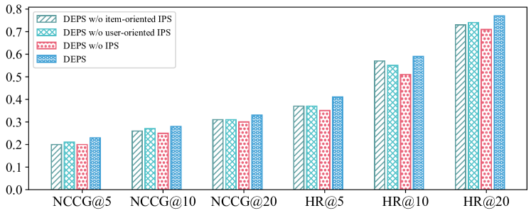
Figure 5. Empirical analysis based on Amazon-Digital Music: DEPS variation performances of NDCG@K and HR@K

5.3. Experimental Analysis

We conducted more experiments to analyze DEPS, based on the Amazon-Digital-Music test data.

5.3.1. Ablation Study

To further show the importance of estimating propensity scores with the two types of sequences from the view of user and the view of item, we also studied their unbiased performance in the second stage of training when the $\mathcal{L}^{unbiased}$ is optimized. Specifically, we showed the NDCG@K and HR@K of several DEPS variations. These variations include learning the recommendation model with no propensity score estimation (denoted as “w/o IPS”), estimating propensity scores with view of item sequences only (“w/o user-oriented IPS”), with the view of user sequences only (“w/o item-oriented IPS”). From the performances shown in Figure 5, we found that (1) “w/o propensity” performed the worst, indicating the importance of propensity scores are in unbiased sequence recommendation; (2) “w/o user-oriented IPS” and “w/o item-oriented IPS” performed much better, indicating that the propensity scores estimated from either of the two views are effective; (3) DEPS with dual propensity scores performed best, verified the effectiveness of DEPS by using both views to conduct the propensity scores estimation.

Table 3. Ablation study on Amazon-Digital-Music test set.

Metric	NDCG@K			HR@K
K	5	10	20	5	10	20
w/o $\mathbf{h}_{u}^{<t}$	0.2161	0.2720	0.3192	0.3599	0.5467	0.7115
w/o $\mathbf{h}_{i}^{<t}$	0.2034	0.2541	0.3035	0.3819	0.5383	0.7253
w/o stage-1	0.1953	0.2423	0.2869	0.3489	0.5082	0.6869
DEPS	0.2256	0.2766	0.3273	0.4093	0.5852	0.7747

Dual-transformer depends on several important mechanisms for estimating propensity scores and learning model parameters, including estimating with the interaction sequences from both $\mathbf{h}_{u}^{<t}$’s and $\mathbf{h}_{u}^{<t}$’s, and using the first stage unsupervised learning for initializing the parameters. Based on the Amazon-Digital-Music dataset, we conducted ablation studies to test the performances of DEPS variations by removing these components shown in Table 3. These DEPS variations include: estimating the propensity scores and conducting recommendation without using $\mathbf{h}_{u}^{<t}$ (denoted as “w/o $\mathbf{h}_{u}^{<t}$”), without using $\mathbf{h}_{i}^{<t}$ (denoted as “w/o $\mathbf{h}_{i}^{<t}$”), and training by skipping the first stage tuning (denoted “w/o stage-1”).

Table 4. Performance comparisons between DEPS and non-sequential IPS methods on Amazon-Digital-Music test set.

Metric	NDCG@K			HR@K
K	5	10	20	5	10	20
Item-Pro	0.1984	0.2385	0.1928	0.3819	0.5220	0.7170
User-Pro	0.2044	0.2494	0.2983	0.3681	0.5275	0.7088
Item-User-Pro	0.2133	0.2665	0.3156	0.3736	0.5495	0.7273
DEPS	0.2256	0.2766	0.3273	0.4093	0.5852	0.7747

According to the results reported in Table 3, we found that compared with the original DEPS, the performances of all DEPS variations dropped, indicating the importance of these mechanisms. Specifically, we found that the performances dropped a lot when either sequence of $\mathbf{h}_{u}^{<t}$’s or $\mathbf{h}_{i}^{<t}$’s were removed from the model, verified the importance of estimating propensity scores from both views simultaneously in sequence recommendation. The results also indicate that the first stage of unsupervised learning did enhance recommendation accuracy.

5.3.2. Influence of Sequential IPS Estimation Methods

In this section, we study the influence of sequential IPS estimation methods compared to non-sequential IPS estimation methods. In our model, the user-oriented and item-oriented IPS are estimated through GRU. We compared it with the non-sequential IPS estimation methods (frequency-based propensity score). The user-oriented IPS are calculated as $p_{u,*}=m_{u}/\max_{u^{\prime}\in\mathcal{I}}m_{u^{\prime}}$ and item-oriented IPS are calculated as $p_{*,i}=m_{i}/\max_{i^{\prime}\in\mathcal{I}}m_{i^{\prime}}$, where $m_{u}$ and $m_{i}$ denotes the interaction numbers of user $u$ and item $i$.

We studied their unbiased performance in the second stage of training when the unbiased loss function $\mathcal{L}^{\textrm{unbiased}}$ is optimized. Specifically, we showed the NDCG@K and HR@K of several DEPS variations, including learning the recommendation model with a single propensity score $p_{*,i}$ (denoted as “Item-Pro”), with a single propensity score $p_{u,*}$ (denoted as “User-Pro”), and with dual propensity scores $p_{*,i},p_{u,*}$ (i.e., replacing estimated propensity score $P(i,\mathbf{h}_{u}^{<t}),P(u,\mathbf{h}_{i}^{<t})$ in DEPS as $p_{*,i},p_{u,*}$ respectively, and denoted as “Item-User-Pro”).

From the performances shown in Table 4, we found that (1) “DEPS” outperformed “Item-User-Pro” by a large margin, indicating the importance of estimating the propensity scores sequentially; (2) “Item-Pro” and “User-Pro” performed worse than “Item-User-Pro”, indicating that the propensity scores estimated from both views (user or item) are effective and complementary.

Table 5. Performance comparisons between DEPS variations where the underlying recommendation model is replaced with GRU4Rec+ or FPMC. Experiments were conducted on Amazon-Digital-Music and ‘$*$’ means the improvements over the underlying models are statistical significant (t-test and $p$-value $<0.05$).

Metric	NDCG@K			HR@K
TopK	5	10	20	5	10	20
GRU4Rec+	0.0651	0.0961	0.1385	0.1709	0.3025	0.4874
DEPS(GRU4Rec+)	0.0861*	0.1219*	0.1608*	0.1905*	0.3272*	0.5182*
FPMC	0.1355	0.1799	0.2153	0.2941	0.4391	0.6091
DEPS(FPMC)	0.1396*	0.1858*	0.2189*	0.3025*	0.4566*	0.6426*

5.3.3. DEPS as a Model-Agnostic Framework

Though DEPS designs a transformer-based model for conducting the recommendation, it can also be used as a model-agnostic framework, by replacing the underlying model (the transformers and the MLP shown in Section 4.3) with other sequential recommendation models. In the experiments, we replaced it with GRU4Rec+ (Tan et al., 2016) and FPMC (Rendle et al., 2010), achieving two new models, denoted as “DEPS (GRU4Rec+)” or “DEPS (FPMC)”, respectively. Please note that the sequential recommendation models of GRU4Rec and FPCM cannot be trained on MLM tasks. Therefore, the loss functions in the first stage training of DEPS (GRU4Rec+) and DEPS (FPMC) degenerates to $\mathcal{L}_{u}^{\text{AR}}+\mathcal{L}_{i}^{\text{AR}}$. From the results reported in Table 5, we found that the DEPS (GRU4Rec+) and DEPS (FPMC) respectively achieved improvements over their underlying models of GRU4Rec+ and FPMC. The results indicate that the propensity scores estimated by DEPS is general. They can be used to improve other sequential recommendation models in a model-agnostic manner.

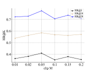
(a) HR@K curve

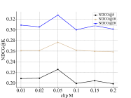
(b) NDCG@K curve

Figure 6. NDCG and HR curves of DEPS w.r.t. clip value $M$

5.3.4. Impact of the Clipping Value M

According to Theorem 2, the clip value $M$ balances the unbiasedness and variance in DEPS. In this experiment, we studied how NDCG@K and HR@K changed when the clip value $M$ was set to different values from $[0.05.0.2]$. From the curves shown in Figure 6, we found the performance improved when $M\in[0.01,0.05]$ and then dropped between $[0.05,0.2]$. The results verified the theoretical analysis that too small $M$ (e.g., $M=0.01$) results in large variance estimation while too large $M$ (e.g., $M=0.2$) results in large bias. It is important to balance the unbiasedness and variance in real applications.

6. Conclusion

This paper proposes a novel IPS estimation method called Dually Enhanced Propensity Score Estimation (DEPS) to remedy the exposure or selection bias in the sequential recommendation. DEPS estimates the propensity scores from the views of item and user and offers several advantages: theoretical soundness, model-agnostic nature, and end2end learning. Extensive experimental results on four real datasets demonstrated that DEPS can significantly outperform the state-of-the-art baselines under the unbiased test settings.

Appendix A Proof of Theorems

A.1. Proof of Theorem 1

Proof.

Let $q_{\mathbf{h}^{<t}_{u},i}\in\{0,1\}$ where $q_{\mathbf{h}^{<t}_{u},i}=1$ indicates item $i$ is observed in the historical interaction sentence $\mathbf{h}^{<t}_{u}$, otherwise $q_{\mathbf{h}^{<t}_{u},i}=0$. According to the definition, $P(q_{\mathbf{h}^{<t}_{u},i}=1)=P(i,\mathbf{h}^{<t}_{u})$ in sequential recommendation. Abbreviate historical information $\mathbf{h}_{u}^{<t},\mathbf{h}_{i}^{<t}$ to $H$. Therefore,

$$\mathbb{E}_{o}\left[\mathcal{L}_{u}\right] =\mathbb{E}_{o}\left[\sum_{u\in\mathcal{U}}\sum_{(i,c_{t})\in\mathcal{D}^{u}}\left[\frac{\delta(c_{t},\hat{r}_{t}(u,i^{t},H))}{P(i^{t},\mathbf{h}^{<t}_{u})}\right]\right]$$

$$=\sum_{u\in\mathcal{U}}\sum_{t:(u,i^{\prime},c_{t})\in\mathcal{D}}\sum_{i\in\mathcal{I}}\mathbb{E}_{q}\left[q_{\mathbf{h}^{<t}_{u},i}\cdot\frac{\delta(r_{t},\hat{r}_{t}(u,i,H))}{P(i,\mathbf{h}^{<t}_{u})}\right]$$

$$=\sum_{u\in\mathcal{U}}\sum_{t:(u,i^{\prime},c_{t})\in\mathcal{D}}\sum_{i\in\mathcal{I}}\delta(r_{t},\hat{r}_{t}(u,i,H))=\mathcal{L}^{\text{ideal}}_{s}$$

Similarly, let $q_{\mathbf{h}^{<t}_{i},u}\in\{0,1\}$ where $q_{\mathbf{h}^{<t}_{i},u}=1$ indicates the user $u$ appeared in the historical interaction sentence $\mathbf{h}^{<t}_{i}$. We have $P(q_{\mathbf{h}^{<t}_{i},u}=1)=P(u,\mathbf{h}^{<t}_{i})$, and

$$\mathbb{E}_{o}\left[\mathcal{L}_{i}\right] =\mathbb{E}_{o}\left[\sum_{i\in\mathcal{I}}\sum_{(i,c_{t})\in\mathcal{D}^{i}}\left[\frac{\delta(c_{t},\hat{r}_{t}(u^{l(i,t+1)},i,H))}{P(u^{l(i,t+1)},\mathbf{h}^{<t}_{i})}\right]\right]$$

$$=\sum_{i\in\mathcal{I}}\sum_{t:(u,i^{\prime},c_{t})\in\mathcal{D}}\sum_{u\in\mathcal{U}}\mathbb{E}_{q}\left[q_{\mathbf{h}^{<t}_{i},u}\frac{\delta(r,\hat{r}(u,i,H))}{P(u,\mathbf{h}^{<t}_{i})}\right]$$

$$=\sum_{u\in\mathcal{U}}\sum_{t:(u,i^{\prime},c_{t})\in\mathcal{D}}\sum_{i\in\mathcal{I}}\delta(r_{t},\hat{r}_{t}(u,i,H))=\mathcal{L}^{\text{ideal}}_{s}.$$

Therefore, $\mathcal{L}^{\mathbf{ideal}}_{s}=\mathbb{E}\left[\mathcal{L}^{\mathbf{unbiased}}_{s}\right]=\mathbb{E}\left[\alpha\mathcal{L}_{u}+(1-\alpha)\mathcal{L}_{i}\right]$ ∎

A.2. Proof of Theorem 2

Proof.

Following the notations defined Theorem 1, we can write $L_{u}^{t}=\frac{\delta(r_{t},\hat{r}_{t})}{p(u,\mathbf{h}^{<t}_{i})}q_{\mathbf{h}^{<t}_{i},u}$, and according to the clip operation shown in Eq. (7) we have $\widetilde{P}(u,\mathbf{h}^{<t}_{i})\geq M$. Therefore,

$$\mathbb{V}\left[L_{u}^{t}\right] =\mathbb{E}\left[L_{u}^{t}\right]^{2}-\left(\mathbb{E}\left[L_{u}^{t}\right]\right)^{2}=\frac{\delta^{2}(r_{t},\hat{r}_{t})}{\widetilde{P}(u,\mathbf{h}^{<t}_{i})}-\delta^{2}(r_{t},\hat{r}_{t})$$

$$=\left(\frac{1}{\widetilde{P}(u,\mathbf{h}^{<t}_{i})}-1\right)\delta^{2}(r_{t},\hat{r}_{t})\leq\left(\frac{1}{M}-1)\delta^{2}(r_{t},\hat{r}_{t})\right).$$

Similarly, we can bound the variance of objective functions $L_{i}^{t}$ as,

$$\mathbb{V}\left[L_{i}^{t}\right]=\left(\frac{1}{\widetilde{P}(i,\mathbf{h}^{<t}_{u})}-1\right)\delta^{2}(r_{t},\hat{r}_{t})\leq\left(\frac{1}{M}-1\right)\delta^{2}(r_{t},\hat{r}_{t}).$$

Applying the Cauchy-Schwarz’ inequality, we can bound the variance of average loss $\mathcal{L}_{s}^{\textrm{unbiased}}=\alpha L_{i}^{t}+(1-\alpha)L_{u}^{t}$ as:

$$\mathbb{V}\left[\mathcal{L}_{s}^{\textrm{unbiased}}\right] =\alpha^{2}\mathbb{V}\left[L_{i}^{t}\right]+(1-\alpha)^{2}\mathbb{V}\left[L_{u}^{t}\right]+2\alpha(1-\alpha)\text{Cov}(L_{i}^{t},L_{u}^{t})$$

$$\leq\alpha^{2}\mathbb{V}\left[L_{i}^{t}\right]+(1-\alpha)^{2}\mathbb{V}\left[L_{u}^{t}\right]+2\alpha(1-\alpha)\sqrt{\mathbb{V}\left[L_{i}^{t}\right]\mathbb{V}\left[L_{u}^{t}\right]}$$

$$\leq\max\left\{\mathbb{V}\left[L_{i}^{t}\right],\mathbb{V}\left[L_{u}^{t}\right]\right\}\leq(\frac{1}{M}-1)\delta^{2}(r,\hat{r}).$$

∎

References

- (1)
- Abdollahpouri and Mansoury (2020) Himan Abdollahpouri and Masoud Mansoury. 2020. Multi-sided Exposure Bias in Recommendation. CoRR abs/2006.15772 (2020).
- Agarwal et al. (2019) Aman Agarwal, Ivan Zaitsev, Xuanhui Wang, Cheng Li, Marc Najork, and Thorsten Joachims. 2019. Estimating position bias without intrusive interventions. In Proceedings of the Twelfth ACM International Conference on Web Search and Data Mining. 474–482.
- Chen et al. (2020a) Jiawei Chen, Hande Dong, Xiang Wang, Fuli Feng, Meng Wang, and Xiangnan He. 2020a. Bias and Debias in Recommender System: A Survey and Future Directions. CoRR abs/2010.03240 (2020).
- Chen et al. (2018) Jiawei Chen, Yan Feng, Martin Ester, Sheng Zhou, Chun Chen, and Can Wang. 2018. Modeling Users’ Exposure with Social Knowledge Influence and Consumption Influence for Recommendation. In Proceedings of the 27th ACM International Conference on Information and Knowledge Management. 953–962.
- Chen et al. (2020b) Jiawei Chen, Can Wang, Sheng Zhou, Qihao Shi, Jingbang Chen, Yan Feng, and Chun Chen. 2020b. Fast adaptively weighted matrix factorization for recommendation with implicit feedback. In Proceedings of the AAAI Conference on Artificial Intelligence, Vol. 34. 3470–3477.
- Chen et al. (2019a) Jiawei Chen, Can Wang, Sheng Zhou, Qihao Shi, Yan Feng, and Chun Chen. 2019a. Samwalker: Social recommendation with informative sampling strategy. In The World Wide Web Conference. 228–239.
- Chen et al. (2019b) Qiwei Chen, Huan Zhao, Wei Li, Pipei Huang, and Wenwu Ou. 2019b. Behavior sequence transformer for e-commerce recommendation in alibaba. In Proceedings of the 1st International Workshop on Deep Learning Practice for High-Dimensional Sparse Data. 1–4.
- Cho et al. (2014) Kyunghyun Cho, Bart van Merrienboer, Çaglar Gülçehre, Dzmitry Bahdanau, Fethi Bougares, Holger Schwenk, and Yoshua Bengio. 2014. Learning Phrase Representations using RNN Encoder-Decoder for Statistical Machine Translation. In Proceedings of the 2014 Conference on Empirical Methods in Natural Language Processing, EMNLP. ACL, 1724–1734.
- Collins et al. (2018) Andrew Collins, Dominika Tkaczyk, Akiko Aizawa, and Joeran Beel. 2018. A study of position bias in digital library recommender systems. arXiv preprint arXiv:1802.06565 (2018).
- Devooght et al. (2015) Robin Devooght, Nicolas Kourtellis, and Amin Mantrach. 2015. Dynamic matrix factorization with priors on unknown values. In Proceedings of the 21th ACM SIGKDD Conference. 189–198.
- Fan et al. (2021a) Xinyan Fan, Zheng Liu, Jianxun Lian, Wayne Xin Zhao, Xing Xie, and Ji-Rong Wen. 2021a. Lighter and better: low-rank decomposed self-attention networks for next-item recommendation. In Proceedings of the 44th International ACM SIGIR Conference on Research and Development in Information Retrieval. 1733–1737.
- Fan et al. (2021b) Ziwei Fan, Zhiwei Liu, Jiawei Zhang, Yun Xiong, Lei Zheng, and Philip S Yu. 2021b. Continuous-time sequential recommendation with temporal graph collaborative transformer. In Proceedings of the 30th ACM CIKM Conference. 433–442.
- Fang et al. (2019) Zhichong Fang, Aman Agarwal, and Thorsten Joachims. 2019. Intervention harvesting for context-dependent examination-bias estimation. In Proceedings of the 42nd International ACM SIGIR Conference on Research and Development in Information Retrieval. 825–834.
- Hu et al. (2008) Yifan Hu, Yehuda Koren, and Chris Volinsky. 2008. Collaborative filtering for implicit feedback datasets. In 2008 Eighth IEEE International Conference on Data Mining. Ieee, 263–272.
- Joachims et al. (2017) Thorsten Joachims, Adith Swaminathan, and Tobias Schnabel. 2017. Unbiased learning-to-rank with biased feedback. In Proceedings of the Tenth ACM International Conference on Web Search and Data Mining. 781–789.
- Kingma and Ba (2015) Diederik P. Kingma and Jimmy Ba. 2015. Adam: A Method for Stochastic Optimization. In 3rd International Conference on Learning Representations.
- Liu et al. (2020) Dugang Liu, Pengxiang Cheng, Zhenhua Dong, Xiuqiang He, Weike Pan, and Zhong Ming. 2020. A general knowledge distillation framework for counterfactual recommendation via uniform data. In Proceedings of the 43rd International ACM SIGIR Conference. 831–840.
- Liu et al. (2018) Qiao Liu, Yifu Zeng, Refuoe Mokhosi, and Haibin Zhang. 2018. STAMP: short-term attention/memory priority model for session-based recommendation. In Proceedings of the 24th ACM SIGKDD. 1831–1839.
- Marlin et al. (2012) Benjamin Marlin, Richard S Zemel, Sam Roweis, and Malcolm Slaney. 2012. Collaborative filtering and the missing at random assumption. arXiv preprint arXiv:1206.5267 (2012).
- Parikh et al. (2016) Ankur Parikh, Oscar Täckström, Dipanjan Das, and Jakob Uszkoreit. 2016. A Decomposable Attention Model for Natural Language Inference. In Proceedings of the 2016 Conference on EMNLP. 2249–2255.
- Paszke et al. (2017) Adam Paszke, Sam Gross, Soumith Chintala, Gregory Chanan, Edward Yang, Zachary DeVito, Zeming Lin, Alban Desmaison, Luca Antiga, and Adam Lerer. 2017. Automatic differentiation in PyTorch. (2017).
- Pearl (2009) Judea Pearl. 2009. Causal inference in statistics: An overview. Statistics surveys 3 (2009), 96–146.
- Qin et al. (2020) Zhen Qin, Suming J Chen, Donald Metzler, Yongwoo Noh, Jingzheng Qin, and Xuanhui Wang. 2020. Attribute-based propensity for unbiased learning in recommender systems: Algorithm and case studies. In Proceedings of the 26th ACM SIGKDD International Conference on Knowledge Discovery & Data Mining. 2359–2367.
- Rendle et al. (2012) Steffen Rendle, Christoph Freudenthaler, Zeno Gantner, and Lars Schmidt-Thieme. 2012. BPR: Bayesian personalized ranking from implicit feedback. arXiv preprint arXiv:1205.2618 (2012).
- Rendle et al. (2010) Steffen Rendle, Christoph Freudenthaler, and Lars Schmidt-Thieme. 2010. Factorizing personalized markov chains for next-basket recommendation. In Proceedings of the 19th international conference on World wide web. 811–820.
- Saito (2020a) Yuta Saito. 2020a. Asymmetric Tri-training for Debiasing Missing-Not-At-Random Explicit Feedback. In Proceedings of the 43rd International ACM SIGIR Conference on Research and Development in Information Retrieval. 309–318.
- Saito (2020b) Yuta Saito. 2020b. Unbiased pairwise learning from biased implicit feedback. In Proceedings of the 2020 ACM SIGIR on International Conference on Theory of Information Retrieval. 5–12.
- Saito et al. (2020a) Yuta Saito, Suguru Yaginuma, Yuta Nishino, Hayato Sakata, and Kazuhide Nakata. 2020a. Unbiased recommender learning from missing-not-at-random implicit feedback. In Proceedings of the 13th International Conference on Web Search and Data Mining. 501–509.
- Saito et al. (2020b) Yuta Saito, Suguru Yaginuma, Yuta Nishino, Hayato Sakata, and Kazuhide Nakata. 2020b. Unbiased recommender learning from missing-not-at-random implicit feedback. In Proceedings of the 13th International Conference on Web Search and Data Mining. 501–509.
- Schnabel et al. (2016) Tobias Schnabel, Adith Swaminathan, Ashudeep Singh, Navin Chandak, and Thorsten Joachims. 2016. Recommendations as treatments: Debiasing learning and evaluation. In ICML. PMLR, 1670–1679.
- Sun et al. (2019) Fei Sun, Jun Liu, Jian Wu, Changhua Pei, Xiao Lin, Wenwu Ou, and Peng Jiang. 2019. BERT4Rec: Sequential recommendation with bidirectional encoder representations from transformer. In Proceedings of the 28th ACM international conference on information and knowledge management. 1441–1450.
- Tan et al. (2016) Yong Kiam Tan, Xinxing Xu, and Yong Liu. 2016. Improved recurrent neural networks for session-based recommendations. In Proceedings of the 1st workshop on deep learning for recommender systems. 17–22.
- Wan et al. (2022) Qi Wan, Xiangnan He, Xiang Wang, Jiancan Wu, Wei Guo, and Ruiming Tang. 2022. Cross Pairwise Ranking for Unbiased Item Recommendation. In Proceedings of the ACM Web Conference 2022. 2370–2378.
- Wang et al. (2022) Zhenlei Wang, Shiqi Shen, Zhipeng Wang, Bo Chen, Xu Chen, and Ji-Rong Wen. 2022. Unbiased Sequential Recommendation with Latent Confounders. In Proceedings of the ACM Web Conference 2022. 2195–2204.
- Wang et al. (2021) Zhenlei Wang, Jingsen Zhang, Hongteng Xu, Xu Chen, Yongfeng Zhang, Wayne Xin Zhao, and Ji-Rong Wen. 2021. Counterfactual data-augmented sequential recommendation. In Proceedings of the 44th International ACM SIGIR Conference on Research and Development in Information Retrieval. 347–356.
- Xue et al. (2017) Hong-Jian Xue, Xinyu Dai, Jianbing Zhang, Shujian Huang, and Jiajun Chen. 2017. Deep Matrix Factorization Models for Recommender Systems.. In IJCAI, Vol. 17. Melbourne, Australia, 3203–3209.
- Zhang et al. (2021b) Shengyu Zhang, Dong Yao, Zhou Zhao, Tat-Seng Chua, and Fei Wu. 2021b. Causerec: Counterfactual user sequence synthesis for sequential recommendation. In Proceedings of the 44th International ACM SIGIR Conference on Research and Development in Information Retrieval. 367–377.
- Zhang et al. (2021a) Yang Zhang, Fuli Feng, Xiangnan He, Tianxin Wei, Chonggang Song, Guohui Ling, and Yongdong Zhang. 2021a. Causal Intervention for Leveraging Popularity Bias in Recommendation. arXiv preprint arXiv:2105.06067 (2021).
- Zhao et al. (2021) Wayne Xin Zhao, Shanlei Mu, Yupeng Hou, Zihan Lin, Yushuo Chen, Xingyu Pan, Kaiyuan Li, Yujie Lu, Hui Wang, Changxin Tian, Yingqian Min, Zhichao Feng, Xinyan Fan, Xu Chen, Pengfei Wang, Wendi Ji, Yaliang Li, Xiaoling Wang, and Ji-Rong Wen. 2021. RecBole: Towards a Unified, Comprehensive and Efficient Framework for Recommendation Algorithms. arXiv:2011.01731 [cs.IR]
- Zheng et al. (2020) Yu Zheng, Chen Gao, Xiang Li, Xiangnan He, Yong Li, and Depeng Jin. 2020. Disentangling user interest and popularity bias for recommendation with causal embedding. arXiv preprint arXiv:2006.11011 (2020).
- Zheng et al. (2021) Yu Zheng, Chen Gao, Xiang Li, Xiangnan He, Yong Li, and Depeng Jin. 2021. Disentangling user interest and conformity for recommendation with causal embedding. In Proceedings of the Web Conference 2021. 2980–2991.
- Zhou et al. (2019) Guorui Zhou, Na Mou, Ying Fan, Qi Pi, Weijie Bian, Chang Zhou, Xiaoqiang Zhu, and Kun Gai. 2019. Deep interest evolution network for click-through rate prediction. In Proceedings of the AAAI conference on artificial intelligence, Vol. 33. 5941–5948.
- Zhou et al. (2018) Guorui Zhou, Xiaoqiang Zhu, Chenru Song, Ying Fan, Han Zhu, Xiao Ma, Yanghui Yan, Junqi Jin, Han Li, and Kun Gai. 2018. Deep interest network for click-through rate prediction. In Proceedings of the 24th ACM SIGKDD International Conference on Knowledge Discovery & Data Mining. 1059–1068.
- Zhou et al. (2020) Kun Zhou, Hui Wang, Wayne Xin Zhao, Yutao Zhu, Sirui Wang, Fuzheng Zhang, Zhongyuan Wang, and Ji-Rong Wen. 2020. S3-rec: Self-supervised learning for sequential recommendation with mutual information maximization. In Proceedings of the 29th ACM International Conference on Information & Knowledge Management. 1893–1902.