The transition to synchronization of networked systems

Abstract

With the only help of eigenvalues and eigenvectors of the graph’s Laplacian matrix, we show that the transition to synchronization of a generic networked dynamical system can be entirely predicted and completely characterized. In particular, the transition is made of a well defined sequence of events, each of which corresponds to either the nucleation of one (or several) cluster(s) of synchronized nodes or to the merging of multiple synchronized clusters into a single one. The network’s nodes involved in each of such clusters can be exactly identified, and the value of the coupling strength at which such events are taking place (and therefore, the complete events’ sequence) can be rigorously ascertained. We moreover clarify that the synchronized clusters are formed by those nodes which are indistinguishable at the eyes of any other network’s vertex, and as so they receive the same dynamical input from the rest of the network. Therefore, such clusters are more general subsets of nodes than those defined by the graph’s symmetry orbits, and at the same time more specific than those described by network’s equitable partitions. Finally, we present large scale simulations which show how accurate are our predictions in describing the synchronization transition of both synthetic and real-world large size networks, and we even report that the observed sequence of clusters is preserved in heterogeneous networks made of slightly non identical systems.

I Introduction

From brain dynamics and neuronal firing, to power grids or financial markets, synchronization of networked units is the collective behavior characterizing the normal functioning of most natural and man made systems [1, 2, 3, 4, 5, 6, 7]. As an order parameter (typically the coupling strength in each link of the network) increases, a transition occurs between a fully disordered and gaseous-like phase (where the units evolve in a totally incoherent manner) to an ordered or solid-like phase (in which, instead, all units follow the same trajectory in time).

The transition between such two phases can be discontinuous and irreversible, or smooth, continuous, and reversible. The first case is known as Explosive Synchronization [8], which has been described in various circumstances [9, 10, 11, 12, 13, 14], and which refers to an abrupt onset of synchronization following an infinitesimally small change in the order parameter, with hysteresis loops that may be observed in a thermodynamic first-order phase transition. The second case is the most commonly observed one, and corresponds instead to a second-order phase transition, resulting in intermediate states emerging in between the two phases. Namely, the path to synchrony [15] is here characterized by a sequence of events where structured states emerge made of different functional modules (or clusters), each one evolving in unison. This is known as cluster synchronization (CS) [16, 17, 18], and a lot of studies pointed out that the structural properties of the graph are responsible for the way nodes cluterize during CS [19, 20, 21, 22]. In particular, it was argued that the clusters formed during the transition are to be connected to the symmetry orbits and/or to the equitable partitions of the graph [20].

In our work, we provide the full elucidation of the transition to synchronization in a network of identical systems, for all possible dynamical systems and all possible network’s architectures. Namely, we introduce a (simple, effective, and limited in computational demand) method which is able to: i) predict the entire sequence of events that are taking place during the transition, ii) identify exactly which graph’s node is belonging to each of the emergent clusters, and iii) provide a rigorous calculation of the critical coupling strength value at which each of such clusters is observed to synchronize. We also demonstrate that such a sequence is in fact universal, in that it is independent on the specific dynamical system operating in each network’s node and depends, instead, only on the graph’s structure. Our study, moreover, allows to clarify that the emerging clusters are those groups of nodes which are indistinguishable at the eyes of any other network’s vertex. This means that all nodes in a cluster have the same connections (and the same weights) with nodes not belonging to the cluster, and therefore they receive the same dynamical input from the rest of the network. As such, we prove theorematically that synchronizable clusters in a network are subsets more general than those defined by the graph’s symmetry orbits, and at the same time more specific than those described by equitable partitions. Finally, we present extensive numerical simulations with both synthetic and real-world networks, which demonstrate how high is the accuracy of our predictions, and also report on synchronization features in heterogenous networks showing that the predicted cluster sequence is maintained even for networks made of non identical dynamical units.

II The synchronization solution

The starting point is a generic ensemble of $N$ identical dynamical systems interplaying over a network $G$. The equations of motion are

$$\dot{\mathbf{x}}_{i} =\mathbf{f}(\mathbf{x}_{i})+d\sum_{j=1}^{N}{\cal L}_{ij}\>\mathbf{g}(\mathbf{x}_{j}),$$ (1)

where $\mathbf{x}_{i}(t)$ is the $m$-dimensional vector state describing the dynamics of each node $i$, $\mathbf{f}:\mathbb{R}^{m}\longrightarrow\mathbb{R}^{m}$ describes the local (identical in all units) dynamical flow, $d$ is a real-valued coupling strength, ${\cal L}_{ij}$ is the $ij$ entry of the Laplacian matrix associated to $G$, and $\mathbf{g}:\mathbb{R}^{m}\longrightarrow\mathbb{R}^{m}$ is the output function through which units interact. ${\cal L}$ is a zero-row matrix, a property which, in turn, guarantees existence and invariance of the synchronized solution $\mathbf{x}_{s}(t)=\mathbf{x}_{1}(t)=\ldots=\mathbf{x}_{N}(t)$.

The necessary condition for the stability of such solution can be assessed by means of the Master Stability Function (MSF) approach, a method initially developed for pairwise coupled systems [23], and later extended in many ways to heterogeneous networks [24], and to time-varying [25, 26] and higher-order [27] interactions. As the MSF is of rather standard use, we decided to convey all details about the associated mathematics in our Supplementary Information text, and to concentrate in the following only in the conceptual steps involved.

The main idea is that one considers a perturbation $\delta{\mathbf{X}}\in\mathbb{R}^{Nm}\equiv(\delta{\mathbf{x}}_{1},\delta{\mathbf{x}}_{2},\dots,\delta{\mathbf{x}_{N}})^{T}$ around the synchronous state (where $\delta\mathbf{x}_{i}=\mathbf{x}_{i}-\mathbf{x}_{s}$ for $i=1,\dots,N$) and performs linear stability analysis of Eq. (1). One has that ${\cal L}$ is a symmetric, zero row sum, matrix. As so, it is diagonalizable, and the set of its eigenvectors forms an orthonormal basis of $\mathbb{R}^{N}$. Then, one calls as $\lambda_{1}\leq\lambda_{2}\leq\lambda_{3}\leq\dots\leq\lambda_{N}$ the strictly real and positive eigenvalues of ${\cal L}$ ordered in size, and as $\mathbf{v}_{1},\mathbf{v}_{2},\dots,\mathbf{v}_{N}$ the associated orthonormal basis of eigenvectors, in the same order. The zero row sum property of ${\cal L}$ implies furthermore that $\lambda_{1}=0$ and that $\mathbf{v}_{1}=\frac{1}{\sqrt{N}}(1,1,\dots,1,1)^{T}$. Therefore, all components of $\mathbf{v}_{1}$ are equal, and this means that $\mathbf{v}_{1}$ is aligned, in phase space, to the synchronization manifold ${\cal M}$, and that an orthonormal basis for the space ${\cal T}$ tangent to ${\cal M}$ is just provided by the set of eigenvectors $\mathbf{v}_{2},\mathbf{v}_{3},\dots,\mathbf{v}_{N}$.

An immediate consequence is that one can expand the error as a linear combination of the eigenvectors $\{\mathbf{v}_{i}\}$ i.e., $\delta{\mathbf{X}}=\sum_{i=1}^{N}{\mathbf{\eta}}_{i}\otimes{\mathbf{v}}_{i}$, where $\otimes$ stands for the direct product. Then, the coefficients $\mathbf{\eta}_{i}\in\mathbb{R}^{m}$ obey $\dot{\mathbf{\eta}_{i}}=\left[J\mathbf{f}(\mathbf{x}_{s})-d\lambda_{i}J\mathbf{g}(\mathbf{x}_{s})\right]\mathbf{\eta}_{i}$, where $J\mathbf{f}(\mathbf{x}_{s})$ and $J\mathbf{g}(\mathbf{x}_{s})$ are, respectively, the $m\times m$ Jacobian matrices of the flow and of the output function, both calculated along the synchronization solution’s trajectory.

The equations for the ${\mathbf{\eta}_{i}}$ are variational, and only differ (at different $i^{\prime}s$) for the eigenvalue $\lambda_{i}$ appearing in the evolution kernel. Therefore, one can separate the structural and dynamical contributions. This is done by introducing a parameter $\nu\equiv d\lambda$, and by studying the variational parametric equation $\dot{\mathbf{\eta}}=\left[J\mathbf{f}(\mathbf{x}_{s})-\nu J\mathbf{g}(\mathbf{x}_{s})\right]\mathbf{\eta}=K(\nu)\mathbf{\eta}$.

Now, the kernel $K(\nu)$ only depends on $\mathbf{f}$ and $\mathbf{g}$ (i.e., on the dynamics), and the structure of the network is encoded within a specific set of $\nu$ values (those obtained by multiplying $d$ times the Laplacian’s eigenvalues).

The maximum Lyapunov exponent $\Lambda$ (i.e., the maximum of the $m$ Lyapunov exponents) can then be computed for each value of $\nu$. The function $\Lambda(\nu)$ is the Master Stability Function (MSF), and only depends on $\mathbf{f}$ and $\mathbf{g}$. At each value of $d$, a given network architecture is just mapped to a set of $\nu\neq 0$ values. The corresponding values of $\Lambda(\nu)$ provide the expansion (if positive) or contraction (if negative) rates in the directions of the eigenvectors $\mathbf{v}_{2},\mathbf{v}_{3},\dots,\mathbf{v}_{N}$, and therefore one needs all these values to be negative in order for ${\cal M}$ to be attractive in all directions of ${\cal T}$.

Now, $\nu=0$ corresponds to $\lambda_{1}=0$ i.e., to the eigenvector $\mathbf{v}_{1}$ aligned with ${\cal M}$. Therefore, $\Lambda(0)$ is equal to the maximum Lyapunov exponent of the isolated system $\dot{\mathbf{x}}=\mathbf{f}(\mathbf{x})$. In turn, this implies that the MSF starts with a value which is strictly positive (strictly equal to 0) if the network’s units are chaotic (periodic).

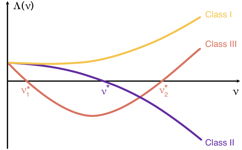
Figure 1: Classes in the Master Stability Function. The maximum Lyapunov exponent $\Lambda$ as a function of the parameter $\nu$ (see text for definitions), for a chaotic flow ($\Lambda(0)>0$). The curve $\Lambda(\nu)$ is called the Master Stability Function (MSF). Given any pair of $\mathbf{f}$ and $\mathbf{g}$, only three classes of systems are possible: Class I systems (yellow line) for which the MSF does not intercept the horizontal axis; Class II systems (violet line), for which the MSF has a unique intercept with the horizontal axis at $\nu=\nu^{*}$ ; Class III systems (brown line), for which the MSF intercepts the horizontal axis at two critical points $\nu=\nu^{*}_{1}$ and $\nu=\nu^{*}_{2}$.

As noticed for the first time in Chapter 5 of Ref. [3], and as illustrated in Fig. 1, all possible choices of (chaotic) flows and output functions, are in fact categorizable into only three classes of systems:

• Class I systems, for which the MSF does not intercept the horizontal axis, like the yellow curve in Fig. 1. These systems intrinsically defy synchronization, because all directions of ${\cal T}$ are always (i.e., at all values of $d$) expanding, no matter which network architecture is used for connecting the nodes. Therefore, neither the synchronized solution $\mathbf{x}_{s}(t)$ nor any other cluster-synchronized state will ever be stable.

• Class II systems, for which the MSF has a unique intercept with the horizontal axis at a critical value $\nu=\nu^{*}$, like the violet line of Fig. 1. The scenario here is the opposite of that of Class I. Indeed, given any network $G$, the condition $d\lambda_{2}>\nu^{*}$ warrants stability of the synchronized solution. These systems, therefore, are always synchronizable, and the threshold for synchronization is $d_{c}\equiv\frac{\nu^{*}}{\lambda_{2}}$ i.e., is inversely proportional to the second smallest eigenvalue of the Laplacian matrix.

• Class III systems, for which the MSF intercepts instead the horizontal axis at two critical points $\nu=\nu^{*}_{1}$ and $\nu=\nu^{*}_{2}$, like the brown V-shaped curve of Fig. 1. In order for the synchronization solution to be stable, it is required in this case that the entire spectrum of eigenvalues of ${\cal L}$ falls (when multiplied by $d$) in between $\nu^{*}_{1}$ and $\nu^{*}_{2}$. In other words, the two conditions $d\lambda_{N}<\nu^{*}_{2}$ and $d\lambda_{2}>\nu^{*}_{1}$ must be simultaneously verified, and this implies that not all networks succeed to synchronize Class III systems. In fact, the former condition gives a bound $d_{\text{m}ax}=\frac{\nu^{*}_{2}}{\lambda_{N}}$ for the coupling strength above which instabilities in tangent space start to occur in the direction of $\mathbf{v}_{N}$, the latter provides once again the threshold $d_{c}\equiv\frac{\nu^{*}_{1}}{\lambda_{2}}$ for complete synchronization to occur.

III The path to synchronization

With all this in mind, let us now move to describe all salient features characterizing the transition to the synchronization solution (as $d$ increases from 0), and in particular to predict all the intermediate events that are taking place during such a transition. Since now, we anticipate that our results are valid for all systems in Class II, as well as for those in Class III (up to the maximum allowed value of the coupling strength i.e., for $d<\frac{\nu^{*}_{2}}{\lambda_{N}}$).

There are three conceptual steps that need to be made.

The first step is that, as $d$ progressively increases, the eigenvalues $\lambda_{i}$ cross the critical point ($\nu=\nu^{*}$ in Class II, or $\nu=\nu^{*}_{1}$ in Class III) sequentially. The first condition which will be met will be, indeed, $d\lambda_{N}>\nu^{*}$ in Class II ($d\lambda_{N}>\nu^{*}_{1}$ in Class III), while for larger values of $d$ the other eigenvalues will cross the critical point one by one (if they are not degenerate) and in the reverse order of their size.

Therefore, one can use this very same order to progressively unfold the tangent space ${\cal T}$. In particular, at any value of $d$, ${\cal T}$ can be factorized as ${\cal T}^{+}(d)\otimes{\cal T}^{-}(d)$, where ${\cal T}^{+}(d)$ [${\cal T}^{-}(d)$] is the subspace generated by the set of eigenvectors $\{\mathbf{v}_{i}\}$ whose corresponding $d\lambda_{i}$ are below (above) the stability condition, i.e., for which one has $d\lambda_{i}\leq\nu^{*}$ ($d\lambda_{i}>\nu^{*}$) in Class II, or $d\lambda_{i}\leq\nu^{*}_{1}$ ($d\lambda_{i}>\nu^{*}_{1}$) in Class III. In other words, the subspace ${\cal T}^{+}(d)$ [${\cal T}^{-}(d)$] contains only expanding (contracting) directions, and therefore the projection on it of the synchronization error $\delta{\mathbf{X}}$ will exponentially increase (shrink) in size.

The second step consists in taking note that, if one constructs the matrix $V$ having as columns the eigenvectors $\mathbf{v}_{i}=(v_{i1},v_{i2},\dots,v_{iN})$, that is

$$V=\begin{pmatrix}v_{11}&v_{21}&\cdots&v_{N1}\\ v_{12}&v_{22}&\cdots&v_{N2}\\ \vdots&\vdots&\ddots&\vdots\\ v_{1N}&v_{2N}&\cdots&v_{NN}\end{pmatrix},$$ (2)

then the rows of matrix (2) provide an orthonormal basis of $\mathbb{R}^{N}$ as well, since $V^{T}V=\mathbb{I}$ implies $V^{T}=V^{-1}$, and hence also $VV^{T}=\mathbb{I}$.

Therefore, one can now examine the eigenvectors componentwise and, for each eigenvector $\mathbf{v}_{i}$, define the following matrix

$$E_{\lambda_{i}}=\begin{pmatrix}(v_{i1}-v_{i1})^{2}&(v_{i2}-v_{i1})^{2}&\cdots&(v_{iN}-v_{i1})^{2}\\ (v_{i1}-v_{i2})^{2}&(v_{i2}-v_{i2})^{2}&\cdots&(v_{iN}-v_{i2})^{2}\\ \vdots&\vdots&\ddots&\vdots\\ (v_{i1}-v_{iN})^{2}&(v_{i2}-v_{iN})^{2}&\cdots&(v_{iN}-v_{iN})^{2}\end{pmatrix}.$$

Furthermore, following the same sequence which is progressively unfolding ${\cal T}$, one recursively defines the following set of matrices $S_{n}$

$$S_{N}=E_{\lambda_{N}},$$

$$S_{N-1}=S_{N}+E_{\lambda_{N-1}},$$

$$\dots\ ,$$

$$S_{2}=S_{3}+E_{\lambda_{2}},$$

$$S_{1}=S_{2}+E_{\lambda_{1}}.$$

It is worth discussing a few properties of such matrices. First of all, as $\mathbf{v}_{1}$ is aligned with ${\cal M}$, all its components are equal, and therefore $E_{\lambda_{1}}=0$ and $S_{1}=S_{2}$. Second, all the $E$-matrices, and thus all the $S$-matrices, are symmetric, non negative and have all diagonal entries equal to zero. In fact, the off diagonal $ij$ elements of the matrix $S_{n}$ ($n=1,\dots,N$) are nothing but the square of the norm of the vector obtained as the difference between the two vectors defined by rows $i$ and $j$ of matrix (2), truncated to their $n$ last components. As so, the maximum value that any entry $i,j$ may have in the matrices $S_{n}$ is 2, which corresponds to the case in which such two vectors are orthogonal. In particular, all off-diagonal entries of $S_{2}=S_{1}$ are equal to 2.

The third conceptual step consists in considering the fact that the Laplacian matrix ${\cal L}$ uniquely defines $G$, and as so any clustering property of the network $G$ has to be reflected into a corresponding spectral feature of ${\cal L}$ [28, 29]. In this paper, we prove rigorously that the synchronized clusters emerging during the transition of $G$ can be associated to a localization of a group of the Laplacian eigenvectors on the clustered nodes. Namely, let us first define that a subset ${\cal S}\subseteq\{\mathbf{v}_{2},\mathbf{v}_{3},\dots,\mathbf{v}_{N}\}$ consisting of $k-1$ eigenvectors forms a spectral block localized at nodes $\{i_{1},\dots,i_{k}\}$ if

• each eigenvector belonging to ${\cal S}$ has all entries (except $i_{1},i_{2},...,i_{k}$) equal to 0;

• for each other eigenvector $\mathbf{v}$ not belonging to ${\cal S}$, the entries $i_{1},i_{2},\dots,i_{k}$ are all equal i.e., $v_{i_{1}}=v_{i_{2}}=\dots=v_{i_{k}}$.

Moreover, all eigenvectors $\{\mathbf{v}_{2},\mathbf{v}_{3},\dots,\mathbf{v}_{N}\}$ are orthogonal to $\mathbf{v}_{1}$, and therefore the sum of all their entries must be equal to 0.

The main theoretical result underpinning our study is the Theorem stated below.

Theorem. The following two statements are equivalent:

1. All $k$ nodes belonging to a cluster defined by the indices $\{i_{1},\ldots,i_{k}\}$ have the same connections with the same weights with all other nodes not belonging to the cluster, i.e., for any $p,q\in\{i_{1},\ldots,i_{k}\}$ and $j\not\in\{i_{1},\ldots,i_{k}\}$ one has ${\cal L}_{pj}={\cal L}_{qj}$.

2. There is a spectral block ${\cal S}$ made of $k-1$ Laplacian’s eigenvectors localized at nodes $\{i_{1},...,i_{k}\}$.

A group of nodes satisfying condition (1) of the theorem is also called an external equitable cell [30].

The reader interested in the mathematical proof of the theorem is referred to our Supplementary Information. We here concentrate, instead, on the main concepts involved. Conceptually, the first statement of the Theorem is tantamount to assert that the nodes belonging to a given cluster are indistinguishable to the eyes of any other node of the network, but puts no constraints on the way such nodes are connected among them within the cluster. Therefore, fulfillment of the statement is realized by (but not limited to) the case of a network’s symmetry orbit. In other words, the first statement of the theorem says that the clustered nodes receive an equal input from the rest of the network, and therefore (for the principle that a same input will eventually - i.e., at sufficiently large coupling -imply a same output) they may synchronize independently on the synchronization properties of the rest of the graph. Therefore, the intermediate structured states emerging in the path to synchrony of a network are more general than the graph’s symmetry orbits, but more specific than the graph’s equitable partitions.

However, the most relevant consequence of the theorem is that the localization of the eigenvectors’ components implies that the matrices $S_{n}$ may actually display entries equal to 2 also for $n$ strictly larger than 2! Indeed, the ($ij$) entry of the matrices $S_{n}$ is just equal to

$$\sum_{k=n}^{N}(v_{kj}-v_{ki})^{2}.$$

Now, suppose that $\mathcal{S}$ is a spectral block localized at $i$, $j$ and some other nodes. Then, if $\mathbf{v}_{k}$ does not belong to $\mathcal{S}$, the term $(v_{kj}-v_{ki})^{2}=0$, and one has therefore that the $(ij)$-entry of $S_{n}$ has contributions only from those eigenvectors $\mathbf{v}_{n}$ belonging to $\mathcal{S}$. Now, all the times that a localized spectral block ${\cal S}$ is contained in the set of those eigenvectors generating ${\cal T}^{-}(d)$ the corresponding cluster of nodes will emerge as a stable synchronization cluster, because the tangent space of the corresponding synchronized solution (where synchrony is limited to those specific nodes) can be fully disentangled from the rest of ${\cal T}$ and will consist, moreover, of only contractive directions.

IV Complete description of the transition

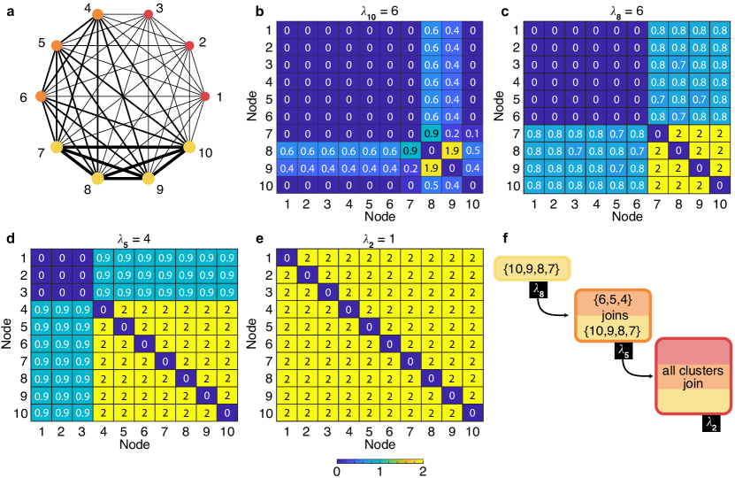
Figure 2: Predicting the transition to synchronization. (a) An all-to-all connected, symmetric, weighted graph of $N=10$ nodes is considered. The graph is endowed with three symmetry orbits: the one composed by the red nodes $\{1,2,3\}$, the one made of the orange nodes $\{4,5,6\}$, and the one made of the four yellow nodes $\{7,8,9,10\}$. In the sketch, the widths of the links are proportional to the corresponding weights, and the sizes of the nodes are proportional to the corresponding strengths. (b) The entries of $S_{10}$, which corresponds to $\lambda_{10}=6$. (c) $S_{8}$ (associated to $\lambda_{8}=6$), where the entries equal to 2 clearly define a cluster formed by nodes $\{7,8,9,10\}$. The first predicted event in the transition then consists in the synchronization of such nodes at $d_{1}=\nu^{*}/\lambda_{8}=\nu^{*}/6$. (d) $S_{5}$ (related to $\lambda_{5}=4$), where additional entries become equal to 2, indicating a second foreseen event in which nodes $\{4,5,6\}$ join the existent synchronization cluster at $d_{2}=\nu^{*}/\lambda_{5}=\nu^{*}/4$. (e) $S_{2}$ (corresponding to $\lambda_{2}=1$) where it is seen that nodes $\{1,2,3\}$ also join the existing synchronized cluster at $d_{3}=\nu^{*}/\lambda_{2}=\nu^{*}$ in a third predicted event where complete synchronization of the network takes place. (f) The expected events (and their exact sequence) occurring in the path to synchrony of the network’s architecture depicted in panel (a). The bar at the bottom of the Figure gives the color code used in panels (b-e) for matrices’ entries.

All needed ingredients are on the table, and one can now cook the cake! An extremely simple (and computationally low demanding) technique can indeed be introduced, able to monitor and track localization of eigenvectors along the transition, and therefore to completely describe the path to synchronization for any generic network and any generic dynamical system.

The method consists in the following steps:

• given a network $G$, one considers the Laplacian matrix ${\cal L}$, and extracts its $N$ eigenvalues $\lambda_{i}$ (ordered in size) and the corresponding eigenvectors $\{\mathbf{v}_{i}\}$;

• one then calculates the $N$ matrices $E_{\lambda_{i}}$ and $S_{n}$ ($i=1,\dots,N;n=1,\dots,N$);

• one inspects the matrices $S_{n}$ in the same order with which the Laplacian’s eigenvalues (when multiplied by $d$) crosses the critical point $\nu^{*}$ (i.e., $N,N-1,N-2,\dots,2,1$), and looks for entries which are equal to 2;

• when, for the first time in the sequence (say, for index $p$) a entry in matrix $S_{p}$ is (or multiple entries are) found equal to 2, a prediction is made that an event will occur in the transition: the cluster (or clusters) formed by the nodes with labels equal to those of the found entry (entries) will synchronize at the coupling strength value $\nu^{*}/\lambda_{p}$. The inspection of matrices $S_{n}$ then continues, focusing only on the entries different from those already found to be 2 at level $S_{p}$;

• after having inspected all $S_{n}$ matrices, one obtains the complete description of the sequence of events occurring in the transition, with the exact indication of all the values of the critical coupling strengths at which each of such events is occurring. By events, we here mean either the formation of one (or many) new synchronized cluster(s), or the merging of different clusters into a single synchronized one.

Let us now move to illustrate the method in a simple case, in order for the reader to have an immediate understanding (and a full appreciation) of the consequences of the various steps that have been discussed so far. For this purpose, we consider the network sketched in panel (a) of Fig. 2, which consists of an all-to-all connected, symmetric, weighted graph of $N=10$ nodes. By construction, the graph is endowed with three symmetric orbits: the first being composed by the pink nodes $1,2$ and $3$, the second containing the blue nodes $4,5$ and $6$, and the third being made of the four green nodes $7,8,9$ and $10$. The 10 eigenvalues of the Laplacian matrix, when ordered in size, are $\{0,1,1,1,4,4,4,6,6,6\}$.

After calculations of the corresponding eigenvectors, the matrices $E_{\lambda_{i}}$ and $S_{n}$ are evaluated. Then, one starts inspecting matrices $S_{n}$ in the reverse order of the size of the corresponding eigenvalues. Panel (b) of Fig. 2 shows $S_{10}$, which corresponds to $\lambda_{10}=6$, and it can be seen that there are no entries equal to 2 in such a matrix. Nor entries equal to 2 are found in $S_{9}$ (not shown). However, when inspecting $S_{8}$ (which corresponds to $\lambda_{8}=6$), one immediately identifies [panel (c) of Fig. 2] many entries equal to 2, which clearly define a cluster formed by nodes $7,8,9$ and $10$. A prediction is then made that the first event observed in the transition will be the synchronization of such nodes in a cluster, occurring exactly at $d_{1}=\nu^{*}/\lambda_{8}=\nu^{*}/6$.

Then, one continues inspecting the matrices $S_{n}$ and concentrates only on all the other entries. No further entry is found equal to 2 in $S_{7}$, nor in $S_{6}$. When scrutinizing $S_{5}$ [panel (d) of Fig. 2] one sees that other entries becomes equal to 2, and they indicate that the cluster formed by nodes $4,5$ and $6$ will merge at $d_{2}=\nu^{*}/\lambda_{5}=\nu^{*}/4=\frac{3}{2}d_{1}$ with the already existing group of synchronized nodes, forming this way a larger synchronized cluster. No further features are observed in $S_{4}$ and $S_{3}$, while the analysis of $S_{2}$ [panel (e) of Fig. 2] reveals that at $d_{3}=\nu^{*}/\lambda_{2}=\nu^{*}=4d_{2}$ also nodes $1,2$ and $3$ join the existing cluster, determining the setting of the final synchronized state, where all nodes of the network evolve in unison.

Panel (f) of Fig. 2 schematically summarizes the predicted sequence of events: if a dynamical system is networking with the architecture of panel (a) of Fig. 2, its path to synchrony will first (at $d=d_{1}$) see the formation of the synchronized cluster $\{7,8,9,10\}$, then (at $d=d_{2}$) nodes $\{4,5,6\}$ will join that cluster, and eventually (at $d=d_{3}$) all nodes will synchronize. Already at this stage it should be remarked that all predictions made are totally independent on $\mathbf{f}$ and $\mathbf{g}$: changing the dynamical system $\mathbf{f}$ operating on each node and/or the output function $\mathbf{g}$ will result in exactly the same sequence of events. The only different will be that the values $d_{i}$ at which the $i^{th}$ event will occur will be rescaled with the corresponding value of $\nu^{*}$.

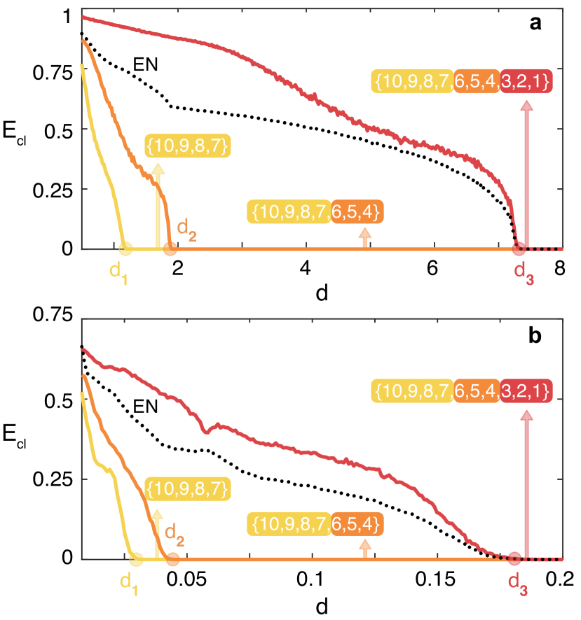
Figure 3: The numerical verification of the predicted transition. The normalized synchronization errors $E_{cl}$ (see text for definition) as a function of $d$, for the Lorenz [panel (a)] and the Rössler [panel (b)] case (see text for the differential equations defining both systems). Data refers to ensemble averages over 500 different numerical simulations of the network sketched in panel (a) of Fig. 2. Cluster 1 (yellow line) is formed by nodes $\{7,8,9,10\}$, Cluster 2 (orange line) is formed by nodes $\{4,5,6\}$, and Cluster 3 (red line) is formed by nodes $\{1,2,3\}$. The black dotted line refers to the synchronization error of the entire network (EN). In both panels it is seen that the expected sequence of events taking place during the transition is verified perfectly. Furthermore, the values $d_{1}=7.322/6=1.220$ ($d_{1}=0.179/6=0.0298$), $d_{2}=7.322/4=1.8305$ ($d_{2}=0.179/4=0.04475$) and $d_{3}=7.322$ ($d_{3}=0.179$) are marked in the horizontal axis respectively with a yellow, orange, and red filled dot in panel (a) (in panel (b)), indicating how accurate are the predictions made on the corresponding critical values for the coupling strength. For each interval, the arrow points to the composition of the synchronized cluster that is being observed, once again in perfect harmony with the predictions made. Finally, we have verified that no extra synchronization features emerge during the transition, other than those explicitly foreseen in Fig. 2.

In order to show how factual is our prediction, we monitored the transition in numerical simulations of Eq. (1), by using the Laplacian matrix of the network of panel (a) of Fig. 2, and by considering two different dynamical systems: the Rössler [31] and the Lorenz system [32] with proper output functions [33]. Precisely, the case of the Rössler system corresponds to $\mathbf{x}\equiv(x,y,z),\ \mathbf{f}(\mathbf{x})=(-y-z,x+ay,b+z(x-c))$ and $\mathbf{g}(\mathbf{x})=(0,y,0)$, while the case of the Lorenz system corresponds to $\mathbf{x}\equiv(x,y,z),\ \mathbf{f}(\mathbf{x})=(\sigma(y-z),x(\rho-z)-y,xy-\beta z)$ and $\mathbf{g}(\mathbf{x})=(x,0,0)$. When parameters are set to $a=0.1,b=0.1,c=18,\sigma=10,\rho=28,\beta=2$, both systems are chaotic and belong to Class II, with $\nu^{*}=7.322$ for the Lorenz case and $\nu^{*}=0.179$ for the Rössler case.

On the other hand, in order to properly quantify synchronization, one calculates the synchronization error over a given cluster, as

$$E_{cl}=\left<\left(\frac{1}{N_{cl}}\sum_{i}\mid\mathbf{x}_{i}-\bar{\mathbf{x}}_{cl}\mid^{2}\right)^{\frac{1}{2}}\right>_{\Delta T},$$ (3)

where the sum runs over all nodes $i$ forming the cluster, $\langle\dots\rangle_{\Delta T}$ stands for a temporal average over a suitable time span $\Delta T$, $\bar{\mathbf{x}}_{cl}$ is the average value of the vector $\mathbf{x}$ in the cluster, and $N_{cl}$ is the number of nodes in the cluster. In addition, the synchronization error is normalized to its maximum value, so as to range from 1 to 0 [34].

The results are reported in Fig. 3, where the normalized synchronization errors is reported as a function of $d$ (for both the Lorenz and the Rössler case) for the entire network (black dotted line) and for each of the three orbits in the network (yellow, orange and red lines). It is clearly seen that all predictions made are fully satisfied.

V Synthetic networks of large size

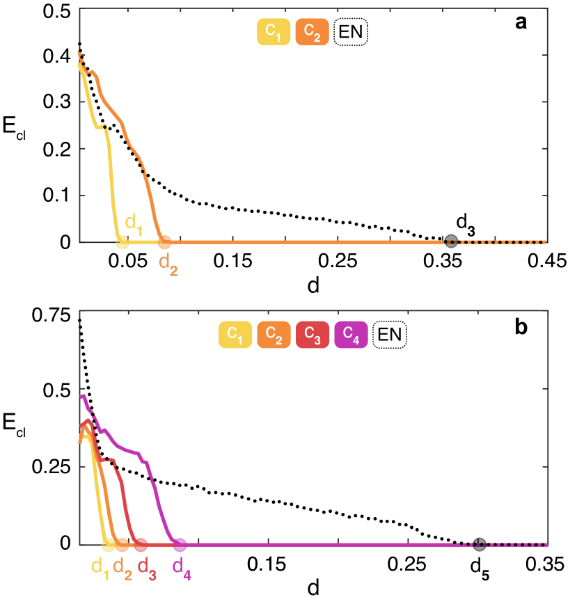
Figure 4: Applications to large size synthetic networks. $E_{cl}$ (see text for definition) vs. $d$, for the Rössler system (see the differential equations in the text). Data in panel (a) [in panel (b)] refer to ensemble averages over 50 (150) different numerical simulations of the graph $G_{1}$ ($G_{2}$) described in the main text. In both panels, the legend sets the color code for the curves corresponding to each of the existing clusters $C_{i}$ and to the Entire Network (EN). Once again, the two predicted transitions are perfectly verified. (a) Cluster 1 synchronizes at $d_{1}=0.179/4=0.04475$ (marked with a yellow dot), Cluster 2 synchronizes at $d_{2}=0.179/2=0.0895$ (orange dot), and the entire network synchronizes at $d_{3}=0.179/0.4758=0.376$ (black dot), as predicted. (b) The cluster with 30 nodes synchronizes at $d_{1}=0.179/5=0.0358$ (yellow dot), the cluster with 100 nodes at $d_{2}=0.179/4=0.04475$ (orange dot), the cluster with 300 nodes at $d_{3}=0.179/3=0.0597$ (red dot), the cluster with 1,000 nodes at $d_{4}=0.179/2=0.0895$ (violet dot), and the entire network at $d_{5}=0.179/0.6025=0.297$ (black dot).

The next step is to test the accuracy of the method in the case of large size graphs. To this purpose, we consider 2 networks that were synthetically generated in Refs. [35, 36]. The first network $G_{1}$ is of size $N=1,000$ nodes, and is endowed with two symmetry orbits that generate two distinct clusters of sizes $20$ nodes (Cluster 1) and $10$ nodes (Cluster 2), respectively. The second network $G_{2}$ is made of $N=10,000$ nodes and is endowed with four symmetry orbits generating four clusters of sizes that span more than an order of magnitude (Clusters 1 to 4 contain, respectively, 1,000, 300, 100, and 30 nodes).

Following the expectations which are detailed in the theorems of our Supplementary Information, the calculation of the Laplacian eigenvalues of $G_{1}$ allows one to identify a first group of 19 degenerate eigenvalues $\lambda_{277,278,\dots,295}=4$ and a second group of 9 degenerate eigenvalues $\lambda_{59,60,\dots,67}=2.$ The analysis of the matrices $S_{n}$ then reveals that the first event in the transition is the synchronization of Cluster 1 at $d_{1}=\nu^{*}/4$, followed by the synchronization of Cluster 2 at $d_{2}=\nu^{*}/2=2d_{1}$, this time in a state which is not synchronized with cluster 1, thus determining an overall state where two distinct synchronization clusters coexist. Eventually, the entire network synchronizes at $d_{3}=\nu^{*}/\lambda_{2}=\nu^{*}/0.4758$.

In the case of $G_{2}$, four blocks of degenerate eigenvalues are indeed found in correspondence with the four clusters. The transition predicted by inspection of the matrices $S_{n}$ is characterized by the sequence of five events. First, the cluster with 30 nodes synchronizes at $d_{1}=\nu^{*}/5$. Second, at $d_{2}=\nu^{*}/4$, the cluster with 100 nodes synchronizes. At $d_{3}=\nu^{*}/3$ ($d_{4}=\nu^{*}/2$) also the cluster with 300 nodes (with 1,000 nodes) synchronizes. The four clusters evolve in four different synchronized states. Eventually, at $d_{5}=\nu^{*}/0.6025$ the entire network synchronizes.

We then simulated the Rössler system on $G_{1}$ and $G_{2}$ and reported the results in Fig. 4, which are actually fully confirming the predicted scenarios.

VI Real-world and heterogeneous networks

We move now to show an application to a real-world network.

To that purpose, we have considered the network of the US power grid. The PowerGrid network consists of 4,941 nodes and 6,594 links, and it is publicly available at https://toreopsahl.com/datasets/#uspowergrid. It was already the object of several studies in the literature, the first of which was the celebrated 1998 paper on small world networks [37]. In the PowerGrid network, nodes are either generators, transformators or substations forming the power grid of the Western States of the United States of America, and therefore they have a specific geographical location. Recently, it was proven that a fraction of $16.7\%$ of its nodes are forming non trivial clusters corresponding to symmetry orbits which are small in size, due to the geographical embedding of the graph [29].

Application of our method detects that the synchronization transition is made of a very well defined sequence of events, which involves the emergence of 381 clusters. The clusters that are being formed are all small in size, because of the constraints made by the geographical embedding. In particular, 310 clusters contain only 2 nodes, 49 clusters are made of 3 nodes, 14 clusters are formed by 4 nodes, 4 clusters have 5 nodes, 2 clusters appear with 6 nodes, 1 cluster has 7 nodes, and 1 cluster is made of 9 nodes. The overall number of network’s nodes which get clustered during the transition is 871. A partial list of these clusters (spanning about one order of magnitude in the size of the corresponding eigenvalues) and the various values of coupling strengths at which the different events are predicted is available in Table 1 of the Supplementary Information.

We have then simulated the Rössler system on the PowerGrid network, and monitored the synchronization error on 6 specific clusters (highlighted in red in the list of Table 1 of the Supplementary Material) that our method foresees to emerge during the path to synchrony in a well established sequence and at well specific values of the coupling strength ($d_{1}=0.04475$, $d_{2}=0.0596$, $d_{3}=0.0895$, $d_{4}=0.1294$, $d_{5}=0.179$, $d_{6}=0.3056$) . The values $d_{1},\dots,d_{6}$ are explicitly calculated in the Supplementary Information, and are marked as filled dots in the horizontal axis of Fig. 5 with the same colors identifying the corresponding clusters. Looking at Fig. 5 (a) one sees that, once again, the observed sequence of events perfectly matches the predicted one, with an excellent fit with the values $d_{1},\dots,d_{6}$.

Finally, we test how robust is the predicted scenario against possible heterogeneities present in the network. To this purpose, one again simulates the Rössler system on the PowerGrid network, but this time one distributes randomly different values of the parameter $b$ to different network’s nodes. Precisely, for each node $i$ of the network, one uses a parameter $b_{i}$ in the Rössler equations which is randomly sorted from a uniform distribution in the interval $[0.1-\epsilon,0.1+\epsilon]$, with the extra parameter $\epsilon$ that now quantifies the extent of heterogeneity in the graph. The results are reported in panel (b) of Fig. 5 for $\epsilon=0.01$, corresponding to 10 % of the value ($b=0.1$) which was used for all nodes in the case of identical systems, thus representing a case of a rather large heterogeneity.

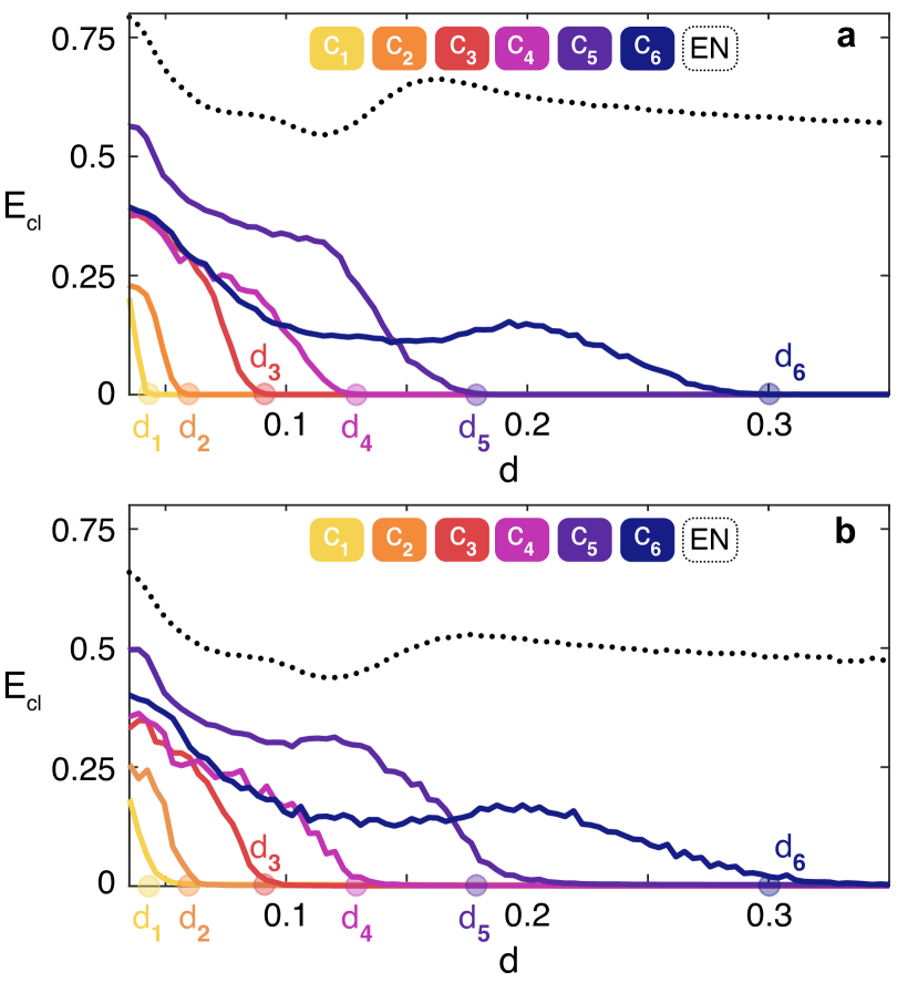
Figure 5: Applications to the PowerGrid network. $E_{cl}$ (see text for definition) vs. $d$, for the Rössler system (see the differential equations in the text). Data in panel (a) [in panel (b)] refer to ensemble averages over 850 (200) different numerical simulations of the PowerGrid network. As in Fig. 4, the legends of both panels set the color code for the curves corresponding to each of the reported clusters $C_{i}$ and to the Entire Network (EN). Panel (a) reports the case of identical Rössler systems, and the error of 6 specific clusters is plotted (see Table 1 of the Supplementary Information for the composition of each of the 6 clusters $C_{i}$). The observed sequence of events perfectly matches the predicted one, with an excellent fit with the values $d_{1},\dots,d_{6}$. In panel (b) the effects of heterogeneity in the network are reported. Namely, for each node $i$ of the PowerGrid network, the parameter $b_{i}$ in the Rössler equations is randomly sorted from a uniform distribution in the interval $[0.1-\epsilon,0.1+\epsilon]$. The curves plotted refer to $\epsilon=0.01$.

It has to be remarked that, when the networked units are not identical, the very same synchronization solution ceases to exist, and therefore it formally makes no sense to speak of the stability of a solution that does not even exist. Indeed, if one selects no matter which ensemble of nodes, the synchronization error never vanishes exactly in the ensemble. Nonetheless, it is still observed that the values of the normalized synchronization errors fluctuate around zero for some sets (clusters) of network’s nodes which, therefore, anticipate the setting of the almost completely synchronized state (wherein all nodes evolve almost in unison). In Fig. 5 (b) it is clearly seen that, while the synchronization errors approach zero at values that are obviously different from those predicted in the case of identical systems, the sequence at which the different clusters emerge during the transition is still preserved. Similar scenarios characterize the evolution of the network also when the heterogeneity is affecting the other two parameters ($a$ and $c$) entering into the equations of the Rössler system.

VII Conclusions

In conclusion, our work gives the complete description of the transition to synchronization in a network of identical systems, for all possible dynamical systems and all possible network’s architectures.

We unveil, indeed, that the path to synchronization is made of a sequence of events, each of which can be exactly identified as either the nucleation of one (or several) cluster(s) of synchronized nodes, or to the merging of multiple synchronized clusters into a single one, or to the growth of an already existing synchronized cluster which enlarges its size.

By combing methodologies borrowed from stability of nonlinear systems with tools of algebra and symmetries, we have been able to introduce a simple and effective method which provides the complete prediction of the sequence of such events, to identify which graph’s node is belonging to each of the emergent clusters, and to give a rigorous forecast of the critical coupling strength values at which such events are taking place.

The results of our manuscript are grounded upon a fully rigorous approach, which demonstrates that the events’ sequence is independent on the specific dynamical system operating in each network’s node and depends, instead, only on the graph’s structure and, more precisely, on the only knowledge of the full spectrum of eigenvalues and eigenvectors of the Laplacian matrix.

Our study, moreover, allows to clarify once forever the intimate nature of the clusters that are being formed along the transition path: they are formed by those nodes which are indistinguishable at the eyes of any other network’s vertex. This implies that nodes in a synchronized cluster have the same connections (and the same weights) with nodes not belonging to the cluster, and therefore they receive the same dynamical input from the rest of the network. Synchronizable clusters in a network are therefore subsets more general than those defined by the graph’s symmetry orbits, and at the same time more specific than those described by equitable partitions.

Finally, our work gave evidence of several extensive numerical simulations with both synthetic and real-world networks, and demonstrates how high is the accuracy of our predictions. Remarkably, the synchronization scenario in heterogenous networks (i.e., networks made of non identical units) preserves the predicted cluster sequence along the entire synchronization path.

Our results provide therefore a full understanding of the transition to synchronization of networked dynamical systems, and call for a lot of applications of general interest in nonlinear science, ranging from synthesizing networks equipped with desired cluster(s) and modular behavior, until predicting the parallel (clustered) functioning of real-world networks from the analysis of their structure.

VIII Acknowledgements

G.C.-A. and K.A.-B. acknowledge funding from projects 2022-SOLICI-120936, 2023/00004/001M2978, and 2023/00005/016M3033 (URJC Grants). G.C.-A. acknowledges funding from the URJC fellowship PREDOC-21-026-2164.

IX Author contributions

S.B. and S.J. designed the research project. A.B., F.N., G.C.-A. and K.A.-B. performed the simulations, K.K. and R.S.-G. developed the mathematical formalism. S.B. and S.J. jointly supervised the research. All authors jointly wrote and reviewed the manuscript.

X Competing interests

The authors declare no competing interests.

In this Supplementary Information (SI), the reader finds all details of the Master Stability Approach, which is used in the first part of the main text, and of our theorem relating the composition of clusters that support synchronization during the transition and the properties of the graph’s Laplacian matrix.

In what follows we consider a connected weighted undirected graph $G$ made of $N$ nodes and uniquely identified by its adjacency matrix $A$ and its Laplacian matrix ${\cal L}$. Furthermore, we will call $\lambda_{1}=0<\lambda_{2}\leq\lambda_{3}\ldots\leq\lambda_{N}$ the (ordered in size) real and positive eigenvalues of ${\cal L}$, and $\mathbf{v}_{1}=\frac{1}{\sqrt{N}}(1,1,1,\ldots,1)^{T},\mathbf{v}_{2},\mathbf{v}_{3},\ldots,\mathbf{v}_{N}$ the corresponding orthonormal eigenvectors. Finally, $V$ will be the matrix having as columns the eigenvectors $\mathbf{v}_{1},\ldots,\mathbf{v}_{N}$.

XI The Master Stability Function Approach

In the first part of the main text, the reader finds a rather extensive discussion on the Master Stability Function Approach and its Classes. Here below, we give all details related to the derivation of such a function.

The equation of motion governing a generic ensemble of $N$ identical dynamical systems interplaying over the network $G$ are

$$\dot{\mathbf{x}}_{i} =\mathbf{f}(\mathbf{x}_{i})+d\sum_{j=1}^{N}{\cal L}_{ij}\>\mathbf{g}(\mathbf{x}_{j}),$$ (4)

where $\mathbf{x}_{i}(t)$ is a $m$-dimensional vector state describing the dynamics of each node $i$, $\mathbf{f}:\mathbb{R}^{m}\longrightarrow\mathbb{R}^{m}$ is the local (identical in all units) dynamical flow describing the evolution of the isolated systems, $d$ is a real-valued coupling strength, ${\cal L}_{ij}$ is the $ij$ entry of the Laplacian matrix, and $\mathbf{g}:\mathbb{R}^{m}\longrightarrow\mathbb{R}^{m}$ is an output function describing the functional way through which units interplay.

${\cal L}$ is a zero-row matrix, a property which, in turn, guarantees existence and invariance of the synchronized solution

$$\mathbf{x}_{s}(t)=\mathbf{x}_{1}(t)=\ldots=\mathbf{x}_{N}(t).$$

In order to study stability of such a solution, one considers perturbations $\delta\mathbf{x}_{i}=\mathbf{x}_{i}-\mathbf{x}_{s}$ for $i=1,...,N$, and performs linear stability analysis of Eq. (4). The result are the following equations:

$$\dot{\delta\mathbf{x}}_{i} =J\mathbf{f}(\mathbf{x}_{s}){\delta\mathbf{x}}_{i}+d\sum_{j=1}^{N}{\cal L}_{ij}\>J\mathbf{g}(\mathbf{x}_{s}){\delta\mathbf{x}}_{j},$$ (5)

where $J\mathbf{f}(\mathbf{x}_{s})$ and $J\mathbf{g}(\mathbf{x}_{s})$ are, respectively, the $m\times m$ Jacobian matrices of the flow and of the output function, both evolving in time following the synchronization solution’s trajectory.

One can, in fact, consider the global error $\delta{\mathbf{X}}\in\mathbb{R}^{Nm}\equiv(\delta{\mathbf{x}}_{1},\delta{\mathbf{x}}_{2},...,\delta{\mathbf{x}_{N}})^{T}$ around the synchronous state, and recast Eqs. (5) as

$$\dot{\delta\mathbf{X}} =\left[J\mathbf{f}(\mathbf{x}_{s})\otimes{\mathbb{I}}+d{\cal L}\otimes J\mathbf{g}(\mathbf{x}_{s})\right]\delta\mathbf{X},$$ (6)

where ${\mathbb{I}}$ is the identity matrix, and $\otimes$ stands for the direct product.

Now, ${\cal L}$ is a symmetric, zero row sum, matrix. As so, it is always diagonalizable, and the set of its eigenvectors forms an orthonormal basis of $\mathbb{R}^{N}$. The zero row sum property of ${\cal L}$ implies furthermore that $\lambda_{1}=0$ and that $\mathbf{v}_{1}=\frac{1}{\sqrt{N}}(1,1,....,1,1)^{T}$. Therefore, all components of $\mathbf{v}_{1}$ are equal, and this means that $\mathbf{v}_{1}$ is aligned, in phase space, to the manifold ${\cal M}$ defined by the synchronization solution, and that an orthonormal basis for the space ${\cal T}$ tangent to ${\cal M}$ is just provided by the set of eigenvectors $\mathbf{v}_{2},\mathbf{v}_{3},...,\mathbf{v}_{N}$. For the synchronization solution to be stable, the necessary condition is then that all directions of the tangent space be contractive.

One can now expand the error $\delta{\mathbf{X}}$ as a linear combination of the eigenvectors $\{\mathbf{v}_{i}\}$ i.e.,

$$\delta{\mathbf{X}}=\sum_{i=1}^{N}{\mathbf{\eta}}_{i}\otimes{\mathbf{v}}_{i}.$$

Then, plugging the expansion in Eq. (6) and operating the scalar product of both the right and left part of the equation times the eigenvectors $\mathbf{v}_{i}$, one obtains that the coefficients $\mathbf{\eta}_{i}\in\mathbb{R}^{m}$ obey the equations

$$\dot{\mathbf{\eta}_{i}}=\left[J\mathbf{f}(\mathbf{x}_{s})-d\lambda_{i}J\mathbf{g}(\mathbf{x}_{s})\right]\mathbf{\eta}_{i}.$$

Notice that the equations for the coefficient ${\mathbf{\eta}_{i}}$ are variational, and only differ (at different $i^{\prime}s$) for the eigenvalue $\lambda_{i}$ appearing in the evolution kernel. This entitles one to cleverly separate the structural and dynamical contributions, by introducing a parameter $\nu\equiv d\lambda$, and by studying the $m$-dimensional parametric variational equation

$$\dot{\mathbf{\eta}}=\left[J\mathbf{f}(\mathbf{x}_{s})-\nu J\mathbf{g}(\mathbf{x}_{s})\right]\mathbf{\eta}=K(\nu)\mathbf{\eta}.$$ (7)

The kernel $K(\nu)$, indeed, only depends on $\mathbf{f}$ and $\mathbf{g}$ (i.e., on the dynamics), and the structure of the network is now encoded within a specific set of $\nu$ values (those obtained by multiplying $d$ times the Laplacian’s eigenvalues).

The maximum Lyapunov exponent $\Lambda$ [(i.e., the maximum of the $m$ Lyapunov exponents of Eq. (7)] can then be computed for each value of $\nu$. The function $\Lambda(\nu)$ is called the Master Stability Function, and only depends on $\mathbf{f}$ and $\mathbf{g}$. At each value of $d$, a given network architecture is just mapped to a set of $\nu\neq 0$ values. The corresponding values of $\Lambda(\nu)$ provide the expansion (if positive) or contraction (if negative) rates in the directions of the eigenvectors $\mathbf{v}_{2},\mathbf{v}_{3},...,\mathbf{v}_{N}$, and therefore one needs all these values to be negative in order for ${\cal M}$ to be attractive in all directions of ${\cal T}$.

Finally, notice that $\nu=0$ corresponds to $\lambda_{1}=0$ i.e., to the eigenvector $\mathbf{v}_{1}$ aligned with ${\cal M}$. Therefore, $\Lambda(0)$ is equal to the maximum Lyapunov exponent of the isolated system $\dot{\mathbf{x}}=\mathbf{f}(\mathbf{x})$. In turn, this implies that the Master Stability Function starts with a value which is strictly positive (strictly equal to 0) if the networks units are chaotic (periodic).

The 3 different Classes of systems supported by the Master Stability Function are illustrated in Fig. 1 of the main text, and largely discussed in our Manuscript.

XII The clusters emerging in the transition to synchronization and the structural properties of the network

This is the central Section of our Supplementary Information, where we give the mathematical proofs of the results stated in the main text about the nature of the clusters observed during the transition to synchronization.

Definition XII.1.

A subset ${\cal S}\subseteq\{\mathbf{v}_{2},\ldots,\mathbf{v}_{N}\}$ consisting of $k-1$ Laplacian eigenvectors is called a spectral block localized at nodes $\{i_{1},\ldots,i_{k}\}$ if

• each eigenvector from this set has all entries except $i_{1},i_{2},\ldots,i_{k}$ equal to $0$;

• any eigenvector $\mathbf{v}_{i}$ not belonging to this set has the entries $i_{1},i_{2},\ldots,i_{k}$ all equal, i.e. $v_{i_{1}}=v_{i_{2}}=\ldots=v_{i_{k}}$.

Note that, since all eigenvectors $\mathbf{v}_{2},\ldots,\mathbf{v}_{N}$ are orthogonal to $\mathbf{v}_{1}$, the sum of all entries of the eigenvectors $\mathbf{v}_{2},\ldots,\mathbf{v}_{N}$ has to be equal to $0$.

Theorem XII.2.

Let $G$ be a connected network with $N$ vertices and Laplacian $\mathcal{L}$ and let $\{i_{1},\ldots,i_{k}\}\subseteq\{1,\ldots,N\}$. Then the following two statements are equivalent:

1. All $k$ nodes belonging to a cluster defined by the indices $\{i_{1},\ldots,i_{k}\}$ have the same connections with the same weights with all other nodes not belonging to the cluster, i.e. for any $p,q\in\{i_{1},\ldots,i_{k}\}$ and $j\not\in\{i_{1},\ldots,i_{k}\}$ one has ${\cal L}_{pj}={\cal L}_{qj}$.

2. There is a spectral block ${\cal S}$ made of $k-1$ Laplacian eigenvectors localized at the nodes $\{i_{1},\ldots,i_{k}\}$.

In this case, starting from a given $n$, the $(p,q)$ entries of the matrices $S_{n}$ defined in the main text will be equal to $2$, for all $p,q\in\{i_{1},\ldots,i_{k}\}$, $p\neq q$. Moreover, the eigenvalues corresponding to this spectral block will only depend on the subgraph induced by the nodes $\{i_{1},\ldots,i_{k}\}$ and the total added degree from all other nodes of the network.

Proof.

Without loss of generality, we can assume $\{i_{1},\ldots,i_{k}\}=\{1,\ldots,k\}$.

$1\Longrightarrow 2$ Consider the $(k-1)$-dimensional subspace $U$ formed by the vectors ${\mathbf{u}}=(u_{1},u_{2},\ldots,u_{N})^{T}\in\mathbb{R}^{N}$ for which $u_{j}=0$ for all $j>k$ and the sum of all entries is equal to $0$, that is,

$$U=\left\{(u_{1},u_{2},\ldots,u_{N})^{T}\in\mathbb{R}^{N}\mid u_{j}=0\text{ for all }j>k\text{ and }\sum_{j=1}^{N}u_{j}=0\right\}.$$ (8)

This is indeed a $(k-1)$-dimensional subspace with (orthogonal) basis $\{\mathbf{e}_{2},\ldots,\mathbf{e}_{k}\}$, where $\mathbf{e}_{i}$ are those vectors where the unique non-zero entries are 1 at position 1 and $-1$ at position $i$. We want to show that $U$ is an invariant subspace of ${\cal L}$, that is, $\mathcal{L}\mathbf{u}\in U$ for all $\mathbf{u}\in U$.

Let $\mathbf{u}=(u_{1},u_{2},\ldots,u_{N})^{T}\in U$ and $j>k$. Then, the $j$-th entry of $\mathcal{L}\mathbf{u}$ is equal to

$$\sum_{i=1}^{N}{\cal L}_{ji}u_{i}=\sum_{i=1}^{k}{\cal L}_{ji}u_{i}.$$ (9)

By hypothesis, we have that ${\cal L}_{ji}={\cal L}_{ij}=a$ for all $i\in\{1,\ldots,k\}$, and hence

$$\sum_{i=1}^{k}{\cal L}_{ji}u_{i}=a\sum_{i=1}^{k}u_{i}=a\cdot 0=0.$$ (10)

It means that every entry of ${\cal L}\mathbf{u}$ after the $k$-th is $0$. The second part (the sum of all the entries of the vector $\mathcal{L}\mathbf{u}$ is zero) holds for any vector: the column (or row) sum of $\mathcal{L}$ is zero, that is, $\mathbf{1}_{N}\mathcal{L}=\mathbf{0}_{N}$, which implies $\mathbf{1}_{N}\mathcal{L}\mathbf{u}=\mathbf{0}_{N}$ for any vector $\mathbf{u}$, where $\mathbf{1}_{N}$ ($\mathbf{0}_{N}$) is a $N$-dimensional vector made of all entries equal to 1 (0).

Consider now $L^{\prime}$, the $k\times k$ principal submatrix of $\mathcal{L}$ given by the first $k$ rows and columns. If $\mathbf{u}\in U$, then $\mathbf{u}=(\mathbf{u}^{\prime}|\mathbf{0}_{N-k})^{T}$ and we can write, in matrix block form,

$$\mathcal{L}\mathbf{u}=\left(\begin{array}[]{c|c}L^{\prime}&A\\ \hline\cr B&C\end{array}\right)\left(\begin{array}[]{c}\mathbf{u}^{\prime}\\ \hline\cr\mathbf{0}\end{array}\right)=\left(\begin{array}[]{c}L^{\prime}\mathbf{u}^{\prime}\\ \hline\cr B\mathbf{u}^{\prime}\end{array}\right)=\left(\begin{array}[]{c}L^{\prime}\mathbf{u}^{\prime}\\ \hline\cr\mathbf{0}\end{array}\right)\in U.$$ (11)

In particular, $\mathcal{L}\mathbf{u}=\lambda\mathbf{u}$ if and only if $L^{\prime}\mathbf{u}^{\prime}=\lambda\mathbf{u}^{\prime}$.

Consider now the graph $G^{\prime}$ induced by the vertices $1,\ldots,k$. Its Laplacian $L(G^{\prime})$ equals $L^{\prime}$ except for the fact that it has diagonal elements $d_{i}^{\text{int}}$ instead of $d_{i}=d_{i}^{\text{int}}+d_{i}^{\text{ext}}$. By hypothesis, $d_{i}^{\text{ext}}=d$ for all $i\leq k$. All in all, $L(G^{\prime})=L^{\prime}-d\,\mathbb{I}_{k}$ and, in particular, $(\lambda,\mathbf{v})$ is an eigenpair of $L(G^{\prime})$ if and only if $(\lambda+d,\mathbf{v})$ is an eigenpair of $L^{\prime}$.

Let $\mathbf{u}^{\prime}_{1},\ldots,\mathbf{u}^{\prime}_{k}$ be an orthonormal basis of the Laplacian $L(G^{\prime})$ with $\mathbf{u}^{\prime}_{1}$ a constant vector. In particular, the sum of the entries of each $\mathbf{u}^{\prime}_{2},\ldots,\mathbf{u}^{\prime}_{k}$ must be zero. If we define $\mathbf{u}_{i}=(\mathbf{u}^{\prime}_{i}|\mathbf{0}_{N-k})^{T}$ for all $i=2,\ldots,k$, then such vectors are in the subspace $U$ and, following what discussed above, $\mathbf{u}_{2},\ldots,\mathbf{u}_{k}$ are eigenvectors of $\mathcal{L}$. Moreover, the eigenvalues corresponding to $\mathbf{u}_{2},\ldots,\mathbf{u}_{k}$ depend only on the structure of the induced graph $G^{\prime}$ and external added degree $d$.

Let $\mathbf{v}$ be a generic eigenvector of ${\cal L}$ orthogonal to $\mathbf{u}_{2},\ldots,\mathbf{u}_{k}$. Hence, $\mathbf{v}$ should be orthogonal to all vectors of $U$, and since all entries after the $k$-th of all vectors from $U$ are 0, then the scalar product between $\mathbf{v}$ and any vector from $U$ has to be equal to the scalar product of the restriction of these vectors to the first $k$ components. The restricted vectors of $U$ span a $(k-1)$-dimensional subspace, therefore the orthogonal subspace is 1-dimensional, containing therefore scalar multiples of $\mathbf{1}_{k}$. Hence, the coordinates of the restricted vector must be equal, implying that the entries $\{1,\ldots,k\}$ of $\mathbf{v}$ are equal.

$2\Longrightarrow 1$ Without loss of generality, we assume that the last $k-1$ eigenvectors form the spectral block localized at nodes $\{1,\ldots k\}$. Then, the matrix $V$ having the eigenvectors as columns can be written in block form as

$$V=\left(\begin{array}[]{c|c}C&V^{\prime}\\ \hline\cr V^{\prime\prime}&\mathbf{0}_{k-1,N-k}\end{array}\right),$$ (12)

where $V^{\prime}$ and $V^{\prime\prime}$ are $k\times(k-1)$ and $(N-k)\times(N-k+1)$ matrices respectively, $C$ is a $k\times(N-k+1)$ column-constant matrix ($C_{pj}=C_{qj}$ for all $p,q,j$), and $\mathbf{0}_{k-1,N-k}$ is a zero $(k-1)\times(N-k)$ matrix.

If $\Sigma$ is the diagonal matrix of the eigenvalues $\lambda_{1},\lambda_{2},\ldots,\lambda_{N}$, we can write the Laplacian as

$${\cal L}=V\Sigma V^{T}=\left(\begin{array}[]{c|c}C&V^{\prime}\\ \hline\cr V^{\prime\prime}&\mathbf{0}_{k-1,N-k}\end{array}\right)\Sigma\left(\begin{array}[]{c|c}C^{T}&(V^{\prime\prime})^{T}\\ \hline\cr(V^{\prime})^{T}&\mathbf{0}_{k-1,N-k}^{T}\end{array}\right).$$ (13)

In turn, this implies that the connections between the nodes $\{1,\ldots,k\}$ and the nodes $\{k+1,\ldots,N\}$ are described by the submatrix

$$\left(\begin{array}[]{c|c}C&V^{\prime}\end{array}\right)\Sigma\left(\begin{array}[]{c}(V^{\prime\prime})^{T}\\ \hline\cr\mathbf{0}_{k-1,N-k}^{T}\end{array}\right).$$ (14)

In particular, if $1\leq p,q\leq k$ and $j>k$,

$$\mathcal{L}_{pj}=\sum_{i=1}^{N-k+1}C_{pi}\Sigma_{ii}V^{\prime\prime}_{ji}+0=\mathcal{L}_{qj},$$ (15)

since $C_{pi}=C_{qi}$ for all $i\leq N-k+1$.

For the final part of the statement, let us remind the $ij$-th entry of $S_{n}$ is equal to

$$\sum_{k=n}^{N}(v_{kj}-v_{ki})^{2}.$$

Let $i,j$ be any two different nodes at which the spectral block $\mathcal{S}$ is localized. Then, if $\mathbf{v}_{k}$ does not belong to $\mathcal{S}$ the term $(v_{kj}-v_{ki})^{2}$ is equal to $0$. Hence, the $ij$-th entry of $S_{n}$ changes only when $\mathbf{v}_{n}$ belongs to $\mathcal{S}$. So, if $\lambda_{n}$ is greater than the maximum eigenvalue of $\mathcal{S}$ then the $ij$-th entry of $S_{n}$ is 0. On the other hand, if $\lambda_{n}$ is less than the minimal eigenvalue of $\mathcal{S}$ the $ij$-th entry of $S_{n}$ is $2$, as was to be shown. ∎

Actually, to be mathematically correct, the formulation of the second statement of the theorem should be There is an eigenbasis $\mathbf{v}_{1},\ldots,\mathbf{v}_{N}$ and a spectral block $\mathcal{S}$ localized at nodes $i_{1},\ldots,i_{k}$, since it could happen that eigenvectors not from $U$ could have the same eigenvalues as eigenvectors in $\mathcal{S}$, so they could be not orthogonal to $U$. However, such a possibility doesn’t affect the synchronization scenario, so we decided to omit to mention explicitly this extra case for the sake of simplicity.

One important example of equitable cells are symmetry orbits, that is, orbits under the action of the automorphism group of the graph. Moreover, most such orbits in real-world networks are either complete or empty subgraphs with all permutations of the vertices realized as network symmetries. This particular case can be characterised as follows.

Theorem XII.3.

Let $G$ be a connected network with $N$ vertices and Laplacian $\mathcal{L}$ and let $\{i_{1},\ldots,i_{k}\}\subseteq\{1,\ldots,N\}$. Then the following three statements are equivalent:

1. For any pair of vertices indexed in the set $\{i_{1},\ldots,i_{k}\}$ a permutation of this pair preserves the Laplacian of the network.

2. The graph induced by $\{i_{1},\ldots,i_{k}\}$ is either complete or empty, and for any $p,q\in\{i_{1},\ldots,i_{k}\}$ and $j\not\in\{i_{1},\ldots,i_{k}\}$ one has ${\cal L}_{pj}={\cal L}_{qj}$.

3. There is a spectral block $\mathcal{S}$ localized at nodes $i_{1},\ldots,i_{k}$ and all $k-1$ eigenvectors of $\mathcal{S}$ have the same, degenerate, eigenvalue.

In the proof of this theorem we will use the following proposition:

Proposition XII.4.

Let $\sigma$ be a permutation of nodes $\{1,\ldots,N\}$ with permutation matrix $P$. Then the following two statements are equivalent

1. Permutation $\sigma$ preserves $\mathcal{L}$, i.e. $P^{-1}\mathcal{L}P=\mathcal{L}$.

2. For any eigenvector $\mathbf{v}_{i}\in\{\mathbf{v}_{1},\ldots,\mathbf{v}_{N}\}$ with eigenvalue $\lambda_{i}$ the vector $P\mathbf{v}_{i}$ is also eigenvector of $\mathcal{L}$ with the same eigenvalue $\lambda_{i}$.

Proof of the Proposition XII.4.

$1\Longrightarrow 2$ Let us consider any eigenvector $\mathbf{v}$ of $\mathcal{L}$ with an eigenvalue $\lambda$. Then

$$\mathcal{L}P\mathbf{v}=PP^{-1}\mathcal{L}P\mathbf{v}=P\mathcal{L}\mathbf{v}=P\lambda\mathbf{v}=\lambda P\mathbf{v}.$$

$2\Longrightarrow 1$ We can write the Laplacian as

$$\mathcal{L}=V\Sigma V^{-1}.$$

Then, the vectors $\{P\mathbf{v}_{1},P\mathbf{v}_{2},\ldots,P\mathbf{v}_{N}\}$ are orthonormal eigenvectors with the same values $\lambda_{1},\lambda_{2},\ldots,\lambda_{N}$. So, we can diagonalize the Laplacian matrix using these eigenvectors. The matrix having $P\mathbf{v}_{1},P\mathbf{v}_{2},\ldots,P\mathbf{v}_{N}$ as columns is equal to $PV$, so

$$\mathcal{L}=(PV)\Sigma(PV)^{-1}=P(V\Sigma V^{-1})P^{-1}=P\mathcal{L}P^{-1}$$

which is equivalent to $\mathcal{L}P=P\mathcal{L}$ and $P^{-1}\mathcal{L}P=\mathcal{L}$.

∎

Proof of the Theorem XII.3.

Without loss of generality, we can assume $\{i_{1},\ldots,i_{k}\}=\{1,\ldots,k\}$.

$1\Longleftrightarrow 2$ One can permute vertices $i,j$ if and only if for any vertex $p\in\{1,\ldots,N\}$ one has ${\cal L}_{ip}={\cal L}_{jp}$. Hence, one can permute any $i,j\in\{1,\ldots,k\}$ if and only if for any $i,j\in\{1,\ldots,k\}$ and any $p\in\{1,N\}$ one has ${\cal L}_{ip}={\cal L}_{jp}$. So, one just needs to show that vertices $\{1,\ldots,k\}$ form a clique. And indeed, for any $i_{1},j_{1},i_{2},j_{2}\in\{1,\ldots,k\}$ one has ${\cal L}_{i_{1}j_{1}}={\cal L}_{i_{2}j_{1}}={\cal L}_{i_{2}j_{2}}$.

$2\Longrightarrow 3$ Theorem XII.2 guarantees that one has a spectral block localized at nodes $1,\ldots,k$, and it remains to show that all the corresponding eigenvalues are the same. Define the subspace $U$ as in the proof of Theorem XII.2. This subspace is generated by the vectors $\{\mathbf{e}_{i}\}_{i=2}^{k}$ such that for $\mathbf{e}_{i}$ entries number $1$ and $i$ are equal to $1$ and $-1$ correspondingly, and all other entries are equal to $0$. Let $\mathbf{u}=(u_{1}\ldots,u_{n})\in U$ be an eigenvector of $\mathcal{L}$ with an eigenvalue $\lambda$. Since $\mathbf{u}$ cannot be constant (the sum of all its entries must be equal to $0$), one can choose $j,l\in\{1,\ldots,k\}$ such that $a=u_{j}\neq u_{l}=b$. Since $1\Longleftrightarrow 2$, we know that the permutation $\sigma=(jl)$ of nodes $j$ and $l$ with permutation matrix $P$ preserves the Laplacian. Using the proof of Proposition XII.4, one then gets that $P\mathbf{u}$ is a $\lambda$-eigenvector. Therefore, $\mathbf{u}^{\prime}=(\mathbf{u}-P\mathbf{u})/(a-b)$ is also a $\lambda$-eigenvector, and only the entries $u^{\prime}_{j}=1$ and $u^{\prime}_{l}=-1$ of $\mathbf{u}^{\prime}$ are not equal to $0$. Using permutations $(1j)$ and $(il)$, one gets that $\mathbf{e}_{i}$ for any $i\in\{1,\ldots,k\}$ is a $\lambda$-eigenvector, and since they generate $U$, all eigenvectors from this spectral block have the same eigenvalue.

$3\implies 1$ Suppose that we have a spectral block $\mathcal{S}$ with one degenerate eigenvalue $\lambda$. The $k-1$ eigenvectors of this spectral block generate a subspace of eigenvectors with eigenvalue $\lambda$ of dimension $k-1$, so this subspace must be equal to $U$ (defined as above). Notice that any permutation $\sigma$ of $\{1,\ldots,k\}$ preserves $U$ and is an identity map for eigenvectors orthogonal to $U$, therefore by the Proposition XII.4 it preservers the Laplacian matrix ${\cal L}$.

∎

A partition of the vertex set of a graph into non-intersecting subsets $\{C_{1},\ldots,C_{r}\}$ is called an equitable partition if for any $i,j\in\{1,\ldots,r\}$ there is a nonnegative integer $b_{ij}$ such that any vertex from $C_{i}$ has exactly $b_{ij}$ neighbors in $C_{j}$ (subsets $C_{1},\ldots,C_{r}$ are called cells). An external equitable partition is defined similarly, except that one only requires the condition for $i\neq j$.

Then, the first statement of Theorem XII.2 can be reformulated as There is an external equitable partition with cells $\{j\mid j\not\in\{i_{1},\ldots,i_{k}\}\}$ and $\{i_{1},\ldots,i_{k}\}$. Therefore, if one has several spectral blocks one can assert that there is an equitable partition where every block has a cell and any two cells $C_{i}$ and $C_{j}$ form a complete bipartite subgraph with equal weights on all edges of this subgraph.

In summary, the condition 1 of the Theorem XII.2 is more general that just a symmetry orbit, but at the same time it is a particular case of equitable partitions. The relevant conclusion is therefore that the clusters observed in the transition to synchronization are more general than the graph symmetry orbits, but more specific than the network equitable partitions.

XIII The synchronization clusters of the PowerGrid network

This final Section contains a large list, which reports the output of the application of the method described in he main text to the PowerGrid network.

In the first column of the list, we report the values of $\lambda$ at which an event of cluster formation occurs along the transition, and the corresponding values of $1/\lambda$ which (once multiplied by $\nu^{*}$) give the critical coupling strength’s values at which such event has to be observed. Each event consists of the simultaneous emergence of synchronization clusters, and the nodes forming each one of them are reported in the second column of the list.

The 6 clusters that are highlighted in red are those whose synchronization error is reported in Fig. 5 of the main text, for a Rössler chaotic system with parameters and coupling function such that it belongs to Class II, displaying $\nu^{*}=0.179$. The predicted critical coupling strengths $d_{1},...,d_{6}$ reported in the horizontal axes of Fig. 5 of the main text are, therefore:

• $d_{1}=0.179*0.25=0.04475$

• $d_{2}=0.179*0.333=0.0596$

• $d_{3}=0.179*0.5=0.0895$

• $d_{4}=0.179*0.723=0.1294$

• $d_{5}=0.179*1=0.179$

• $d_{6}=0.179*1.707=0.3056$

As already discussed in the main text, a total of 381 clusters are found, involving an overall number of 871 network’s nodes which get clustered during the transition: 310 clusters contain only 2 nodes, 49 clusters are made of 3 nodes, 14 clusters are formed by 4 nodes, 4 clusters have 5 nodes, 2 clusters appear with 6 nodes, 1 cluster has 7 nodes, and 1 cluster is made of 9 nodes.

The list reported here below is limited to the first 11 predicted events.

$\lambda$	Clusters
$\begin{array}[]{c}\lambda=4\\ \frac{1}{\lambda}=0.25\end{array}$	[1081,1082] [2638,2640,2641] [2793,2794] [3037,3038] [3089,3090,3092] [3220,3222] [3226,3227] [3249,3250] [3252,3254] [3297,3298,3300] [3349,3350,3351]
$\begin{array}[]{c}\lambda=3\\ \frac{1}{\lambda}=0.333\end{array}$	[346,347] [2012,2013] [2153,2154] [2442,2443] [2452,2453] [2689,2690] [2917,2918] [3057,3058] [3065,3069] [3067,3068] [3075,3076] [3198,3199] [3260,3262] [3283,3284] [3299,3301] [3312,3313] [3319,3320] [3325,3326] [3359,3360] [3651,3652] [4480,4481]
$\begin{array}[]{c}\lambda=2\\ \frac{1}{\lambda}=0.5\end{array}$	[7,8] [122,123] [341,342] [632,633] [638,639] [641,643] [668,781] [860,861] [966,967] [1154,1155] [1476,1478] [1829,1834] [1956,1960] [1957,1961] [1968,2125] [2111,2112] [2184,2186] [2196,2262] [2221,2222] [2284,2285] [2318,2320] [2469,2470] [2489,2490] [2523,2830] [2655,2656] [2664,2665] [2813,2814] [2829,2834] [2841,2842] [2881,2882] [2929,2935] [3030,3031] [3185,3187,3188][3419,3420] [3474,3475] [3538,3539] [3554,3555] [3557,3558] [3726,3727] [3804,3805] [3902,3903] [4162,4163] [4455,4457] [4868,4923]
$\begin{array}[]{c}\lambda=1.753\\ \frac{1}{\lambda}=0.57\end{array}$	[582,586] [585,587] [635,636]
$\begin{array}[]{c}\lambda=1.382\\ \frac{1}{\lambda}=0.723\end{array}$	[1344,1345][1825,1826][1835,1836][2256,2257]
$\begin{array}[]{c}\lambda=1\\ \frac{1}{\lambda}=1\end{array}$	[12,4935] [14,173] [19,21] [32,34] [36,37] [66,154] [86,87,88] [101,102] [109,4510] [133,135,136] [206,207] [213,214,215,216] [218,4523] [248,249] [256,257,258] [284,285] [348,391] [355,357,360,361] [405,406] [416,417] [419,420] [435,436] [461,462,463,464] [468,469] [573,575] [591,592] [593,646] [596,597] [601,4519,4520,4521,4522] [605,607] [647,648] [654,655,656] [683,689] [690,703,704,705,706,707,708] [693,694] [699,700,702] [709,712] [717,719] [759,771] [778,779] [783,784,785] [806,807] [808,809] [825,836] [839,885] [841,842] [858,859] [870,878] [872,874] [912,913] [934,935,939,940,941,942,943,944,945] [981,982,983,984,985] [987,988,989] [1019,1020] [1021,1022] [1025,1026] [1027,1028] [1124,1126] [1131,1132,1133] [1142,1144,1145,1146] [1209,1565,1570] [1228,1230] [1394,1395] [1419,1420] [1481,2276] [1535,1536] [1767,1768] [1837,1838] [1840,1841] [1917,1921] [1935,1936] [2034,2139] [2060,2062] [2169,2170] [2249,2250] [2268,2269] [2272,2273] [2286,2442,2443] [2352,2354] [2386,2387] [2401,2402,2403] [2414,2415] [2449,2450] [2462,2463,2464] [2497,2498] [2553,2555,2562,2563] [2569,2571] [2576,2578] [2635,2636] [2642,2643] [2671,2672] [2705,2706] [2709,2710,2711] [2725,2726,2728] [2730,2731] [2742,2743] [2744,2746] [2748,2749] [2758,2759] [2835,2836,2838] [2839,2840] [2843,2844] [2872,2873] [2904,2905] [2910,2913,2914,2915] [2979,2980] [2997,2998] [3000,3001] [3004,3005,3006,3007,3008,3009] [3011,3012] [3023,3024] [3041,3042,3189,3190] [3054,3268] [3065,3067,3068,3069] [3075,3076,3077] [3080,3081,3082,3083] [3084,3311] [3088,3089,3090,3092] [3104,3105] [3196,3218,3219] [3201,3202] [3260,3261,3262] [3283,3284,3285] [3286,3287] [3288,3289] [3297,3298,3299,3300,3301] [3309,3310] [3318,3347,3364] [3327,3328] [3349,3350,3351,3369] [3363,3365] [3398,3399] [3410,3412,3413,3724] [3435,3436,3437] [3464,3465] [3480,3481] [3484,3485] [3559,3561] [3572,3577,3578] [3609,3632,4918] [3611,3613,3614] [3616,3730] [3619,3620] [3622,3629] [3624,3704] [3625,3801] [3630,3705,3706] [3639,3640] [3658,3660] [3661,3662,3666] [3700,3812] [3717,3718] [3778,3796] [3802,3818] [3809,3810] [3814,3838] [3840,3841] [3878,3879] [3882,3885] [3938,3944] [3946,3947,3948] [4097,4098] [4107,4174] [4110,4111,4113] [4125,4126] [4155,4156] [4171,4172,4173] [4175,4181] [4177,4179] [4195,4197] [4211,4213] [4217,4218,4219] [4223,4224,4225] [4232,4233] [4252,4253] [4262,4263] [4264,4266] [4270,4271] [4282,4283] [4287,4288,4289] [4303,4304,4305] [4307,4308,4309,4310] [4311,4312,4313] [4320,4321] [4325,4326] [4328,4329] [4330,4331] [4336,4337,4338,4339] [4340,4341] [4346,4347,4348,4349] [4351,4352,4353]
	[4354,4355] [4357,4358,4359,4360,4361] [4362,4363] [4365,4366,4367,4368,4369] [4370,4371,4372,4373] [4377,4378,4379,4380,4381,4382] [4384,4385] [4387,4388] [4389,4390,4391] [4393,4394] [4395,4396,4397] [4398,4399] [4400,4401] [4488,4489] [4511,4512] [4513,4515] [4516,4518] [4604,4605] [4643,4647,4648,4649] [4658,4659] [4679,4680,4681] [4684,4685] [4702,4703] [4717,4718,4719] [4729,4730] [4746,4860] [4799,4813] [4800,4802] [4829,4830] [4841,4842] [4843,4844] [4884,4885] [4907,4908]
$\begin{array}[]{c}\lambda=0.6972\\ \frac{1}{\lambda}=1.434\end{array}$	[2774,2939] [2775,2940] [4826,4828] [4827,4850]
$\begin{array}[]{c}\lambda=0.6228\\ \frac{1}{\lambda}=1.606\end{array}$	[614,615] [617,618] [622,623]
$\begin{array}[]{c}\lambda=0.5858\\ \frac{1}{\lambda}=1.707\end{array}$	[564,565,566] [2510,2949] [2511,2627] [2798,2799] [2831,2832,2833] [2852,2853,2854] [2911,2912] [2946,2947] [2964,2965] [3128,3177] [3208,3209] [3211,3212,3213] [3233,3234,3235] [3244,3245,3246] [3279,3280] [3372,3373]
$\begin{array}[]{c}\lambda=0.5188\\ \frac{1}{\lambda}=1.927\end{array}$	[3742,3746,3749][3743,3748,3750][3744,3745,3747]
$\begin{array}[]{c}\lambda=0.3820\\ \frac{1}{\lambda}=2.618\end{array}$	[868,907] [869,904] [1568,1571] [1616,2045] [2750,2774,2939] [2751,2775,2940] [2891,3043] [2892,2894] [2897,2901] [2898,2900] [3146,3150] [3147,3151] [3148,3272] [3149,3273]

References

- [1] A. Pikovsky, M. Rosenblum, and J. Kurths, Synchronization: a universal concept in nonlinear sciences, Vol. 12 (Cambridge University Press, 2003).
- [2] S. Strogatz, Sync: The emerging science of spontaneous order (Penguin UK, 2004).
- [3] S. Boccaletti, V. Latora, Y. Moreno, M. Chavez, and D.-U. Hwang, Complex networks: Structure and dynamics, Physics Reports 424, 175 (2006).
- [4] A. E. Motter, S. A. Myers, M. Anghel, and T. Nishikawa, Spontaneous synchrony in power-grid networks, Nature Physics 9, 191 (2013).
- [5] F. A. Rodrigues, T. K. D. Peron, P. Ji, and J. Kurths, The kuramoto model in complex networks, Physics Reports 610, 1 (2016).
- [6] M. Breakspear, Dynamic models of large-scale brain activity, Nature Neuroscience 20, 340 (2017).
- [7] S. Boccaletti, A.N. Pisarchik, C.I. Del Genio, A. Amann, Syncronization: From Couped Systems to Complex Networks, (Cambridge University Press, 2018).
- [8] S. Boccaletti, J. Almendral, S. Guan, I. Leyva, Z. Liu, I. Sendiña-Nadal, Z. Wang, Y. Zou, Explosive transitions in complex networks’ structure and dynamics: Percolation and synchronization, Physics Reports 660, 1-94 (2016).
- [9] H.-A. Tanaka, A. J. Lichtenberg, S. Oishi, First order phase transition resulting from finite inertia in coupled oscillator systems, Physical Review Letters 78, 2104 (1997).
- [10] D. Pazó, Thermodynamic limit of the first-order phase transition in the Kuramoto model, Physical Review E 72, 046211 (2005).
- [11] J. Gómez-Gardeñes, S. Gómez, A. Arenas, Y. Moreno, Explosive synchronization transitions in scale-free networks, Physical Review Letters 106, 128701 (2011).
- [12] I. Leyva, R. Sevilla-Escoboza, J. Buldú, I. Sendiña-Nadal, J. Gómez-Gardeñes, A. Arenas, Y. Moreno, S. Gómez, R. Jaimes-Reátegui, S. Boccaletti, Explosive first-order transition to synchrony in networked chaotic oscillators, Physical Review Letters 108, 168702 (2012).
- [13] X. Zhang, S. Boccaletti, S. Guan, Z. Liu, Explosive synchronization in adaptive and multilayer networks, Physical Review Letters 114, 038701 (2015).
- [14] T. Wu, S. Huo, K. Alfaro-Bittner, S. Boccaletti, and Z. Liu, Double explosive transition in the synchronization of multilayer networks, Physical Review Research 4, 033009 (2022).
- [15] J. Gómez-Gardeñes, Y. Moreno, and A. Arenas, Paths to synchronization on complex networks, Physical Review Letters 98, 034101 (2007).
- [16] F. Sorrentino and E. Ott, Network synchronization of groups, Physical Review E 76, 056114 (2007).
- [17] C. R. Williams, T. E. Murphy, R. Roy, F. Sorrentino, T. Dahms, and E. Schöll, Experimental observations of group synchrony in a system of chaotic optoelectronic oscillators, Physical Review Letters 110, 064104 (2013).
- [18] P. Ji, T. K. D. Peron, P. J. Menck, F. A. Rodrigues, and J. Kurths, Cluster explosive synchronization in complex networks, Physical Review Letters 110, 218701 (2013).
- [19] V. Nicosia, M. Valencia, M. Chavez, A. Díaz-Guilera, and V. Latora, Remote synchronization reveals network symmetries and functional modules, Physical Review Letters 110, 174102 (2013).
- [20] L. M. Pecora, F. Sorrentino, A. M. Hagerstrom, T. E. Murphy, and R. Roy, Cluster synchronization and isolated desynchronization in complex networks with symmetries, Nature Communications 5, 4079 (2014).
- [21] L. V. Gambuzza and M. Frasca, A criterion for stability of cluster synchronization in networks with external equitable partitions, Automatica 100, 212 (2019).
- [22] F. Della Rossa, L. Pecora, K. Blaha, A. Shirin, I. Klickstein, and F. Sorrentino, Symmetries and cluster synchronization in multilayer networks, Nature Communications 11, 1 (2020).
- [23] L. M. Pecora and T. L. Carroll, Master Stability Functions for Synchronized Coupled Systems, Physical Review Letters 80, 2109 (1998).
- [24] J. Sun, E. M. Bollt, and T. Nishikawa, Master stability functions for coupled nearly identical dynamical systems, Europhysics Letters 85, 60011 (2009).
- [25] S. Boccaletti, D.-U. Hwang, M. Chavez, A. Amann, J. Kurths, and L. M. Pecora, Synchronization in dynamical networks: Evolution along commutative graphs, Physical Review E 74, 016102 (2006).
- [26] C.I. del Genio, M. Romance, R. Criado, and S. Boccaletti, Synchronization in dynamical networks with unconstrained structure switching, Physical Review E 92, 062819 (2015).
- [27] L. V. Gambuzza, F. Di Patti L. Gallo, S. Lepri, M. Romance, R. Criado, M. Frasca, V. Latora, and S. Boccaletti, Stability of synchronization in simplicial complexes, Nature Communications 12, 1255 (2021).
- [28] B.D. MacArthur and R.J. Sánchez-García, Spectral characteristics of network redundancy Physical Review E, 80, 026117 (2009).
- [29] R.J. Sánchez-García, Exploiting symmetry in network analysis, Nature Communications Physics 3, 87 (2020).
- [30] M.T. Schaub, N. O’Clery, Y.N. Billeh, J-C. Delvenne, R. Lambiotte, and M. Barahona, Graph partitions and cluster synchronization in networks of oscillators, Chaos: An Interdisciplinary Journal of Nonlinear Science 26, 094821 (2016).
- [31] O. E. Rössler, An equation for continuous chaos, Physics Letters A 57, 397 (1976).
- [32] E.N. Lorenz, Deterministic nonperiodic flow, Journal of the Atmospheric Sciences 20, 130 (1963).
- [33] Simulations were performed with an adaptative Tsit integration algorithm implemented in Julia. In each trial, the network is simulated for a total period of 1,500 time units, and the synchronization errors are averaged over the last = 100 time units.
- [34] As one is only interested to monitor the vanishing of , with the purpose of saving calculations in all our simulations the synchronization error is computed by only taking into account those variables of the system’s state where the coupling is acting. This implies that, when referring to the Rössler (Lorenz) system, has been evaluated taking into account only the difference (). The results are, indeed, identical to those obtained when all state variables of the systems are accounted for in the evaluation of , as its formal definition of Eq. (3) would instead require.
- [35] P. Khanra, S. Ghosh, K. Alfaro-Bittner, P. Kundu, S. Boccaletti, C. Hens, and P. Pal, Identifying symmetries and predicting cluster synchronization in complex networks, Chaos, Solitons & Fractals 155, 111703 (2022).
- [36] P. Khanra, S. Ghosh, D. Aleja, K. Alfaro-Bittner, G. Contreras-Aso, R. Criado, M. Romance, S. Boccaletti, P. Pal, C. Hens, Endowing networks with desired symmetries and modular behavior, ArXiV 2302.10548 (2023).
- [37] D.J. Watts, and S.H. Strogatz, Collective dynamics of ‘small-world’ networks, Nature 393, 440 (1998).
Supplementary Information