Temperature dependence study of water dynamics in Fluorohectorite clays using Molecular dynamics simulations

Abstract

In this work, we have carried out molecular dynamics (MD) simulation techniques to study the diffusion coefficient of interlayer molecules at different temperature. Within the wider context of water dynamics in soils, and with a particular emphasis on clays, we present here the translational dynamics of water in clays, in a bi-hydrated states. We focus on temperatures between 293 K and 350 K, i.e., the range relevant to the environmental waste packages. A natural hectorite clay of interest is modified as a synthetic clay, which allows us to understand the determinantal parameters from MD simulations through a comparison with the experimental values. The activation energy $E_{a}$ determined by our simulation is $[8.50-16.62]\frac{kJ}{mol}$. The calculated diffusive constants are in the order of 10$\rm{}^{-5}\leavevmode\nobreak\ cm^{2}s^{-1}$. The simulation results are in good agreement with experiments for the relevant set of conditions, and they give more insight into the origin of the observed dynamics.

1 Introduction

Clay minerals are abundant, non-toxic, cheap and reusable [1]. They have large surface areas, making them ideal for applications in which we want to adsorb other molecules on the surface. Because of the layered nature of the structure of these materials, inserting different molecules between layers can result in adsorption with high binding energies. Today, clay, especially smectite clay, are studied for different applications like the possibilities for a carbon storage [2, 1, 3, 4], water retention and adsorpition [5, 6, 7], and drug delivery mechanism [8, 9, 10]. While clay mineral deposits can be found all over the world, their composition and impurities vary. Although kaolins and smectites are widely available in the commercial market, several useful clay minerals are not abundant in nature. Furthermore, two major issues arise in the use of clay minerals. These are the depletion of the natural deposits, especially those with easy access for mining, and the occurrence of this clay as a mixture of several phases instead of a pure single phase. To overcome these problems, scientists in the fields of geology, material science, and geochemistry have been taking particular interest in the laboratory synthesis of clay minerals over recent decades [11, 12, 13]. In this work, we will consider a specific type of clay material in the Synthetic smectite group, called Fluorohectorite. It is an important material in clay science that definitely underlines the statement that ”Clays may be considered as the material of the 21^st century” [14]. Analyzing water dynamics in anisotropic and confined media such as clay minerals is vital for comprehending transport features in such materials as split solids, porous media, soil models, in environmental sciences. Water plays a crucial role for clay materials when it comes to the storage of high radioactive wastes, since the waste is surrounded by water and ions that can disperse inside the clay, in what is called a phenomenon that requires long-term forecasting. This necessitates the understanding of the behaviour of water on several length-scales, the smallest of which is the nanoscale, and also for a range of temperature between 293 K and 350 K.

2 Computational Methods

2.1 System setup

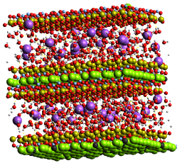
Figure 1: Snapshot of the pre-equilibrated systems with 48 interlayer cation, 480 water molecule with two half, and one full layer hectorite clay. Colors: O (red), H (white), Si (dark yellow), green (Mg), Na (purple), F (lightskyblue).

The unit-cell formula of Fluorohectorite clay is

$$[M_{x}]^{int}[{Mg}_{6-x}{Li}_{x}]^{oct}[{Si}_{8}]^{tet}{O}_{20}F_{4}$$ (1)

where $M$ denotes some form of an intercalated cation between clay layers. In the present work, the intercalated cations considered are monovalent cations such as Li⁺, Na⁺, K⁺, and Cs⁺. The simulation box is shown in Fig. 1, and the corresponding crystallographic positions of the atoms in the clay unit cell are given elsewhere [15]. Certain parameters in real clay, however, remain unknown. These are: the number of H₂O units per cation, the interlayer spacing, and the preferred orientations of adjacent clay surfaces. The sheets of clay are considered as rigid molecules. Our periodic simulation cell has three dimensional periodic boundary conditions. The SPC water model represents the water molecule in this clay-water interaction. The Lennard-Jones (L-J) potential model defines the van der Waals interactions between water-water, water-clay, water-cation, clay-clay, clay-cation, and cation-cation. Summations across all interaction sites yields the total potential energy for the system, where the pair-wise interaction is given by

$$V_{ij}=\frac{q_{i}q_{j}}{4\pi\varepsilon_{0}r_{ij}}+4\varepsilon_{ij}\Bigg{[}\Bigg{(}\frac{\sigma_{ij}}{r_{ij}}\Bigg{)}^{12}-\Bigg{(}\frac{\sigma_{ij}}{r_{ij}}\Bigg{)}^{6}\Bigg{]}$$ (2)

$q_{i}$ and $q_{j}$ are the partial charges carried by the atoms and ${\epsilon}_{ij}$ and ${\sigma}_{ij}$ are the Lennard-Jones parameters obtained from the corresponding atomic parameters using the Lorentz Berthelot mixing rule [16].

$${\varepsilon}_{ij}=\sqrt{{\varepsilon}_{i}{\varepsilon}_{j}}$$ (3)

$\&$

$${\sigma}_{ij}=\frac{{\sigma}_{i}+{\sigma}_{j}}{2}$$ (4)

All of these parameters depend on the force field chosen to describe the system. In our study, we choose the flexible clayFF force field, slightly adapted to our synthetic clay, because it is shown to give transport properties of water, close to experiment. The SPC model for H₂O molecules is preferred to be the TIP4P/2005 model [17]. The TIP4P/2005 water model has a dipole moment of $2.35\leavevmode\nobreak\ D$ and a polarization correction to the total energy of $5.52\leavevmode\nobreak\ {\frac{kg}{mol}}$, which is better as compared to other models [18]. When we simulate a water molecule inside a nanopore, we want to start out with a density close to the density of bulk water, which is ${\rho_{bulk}}=0.99\leavevmode\nobreak\ \frac{g}{{cm}^{3}}$. The distribution of interlayer cation and water perpendicular to the plane of the clay layers are analysed with atomic density profile (z-density plots). Density profiles were generated to investigate the distribution of the various species in the clay’s interlamellar space. The local coordination environment of interlayer ion by the basal oxygen atoms of the clay layer and water molecules (H₂O) are characterized by RDFs. The radial distribution function for species B around species A is calculated as follows,

$$G_{A-B}(r)=\frac{1}{4\pi\rho_{B}r^{2}}\frac{d(N_{A-B})}{dr}$$ (5)

where $\rho_{B}$ is a number density of species B, the fraction $\frac{d(N_{A-B})}{dr}$ is the average number of species particle B, lying in the region $r$ to $r+dr$, to a species particle A, and $N_{A-B}$ is the coordination number for species B around species A. The RDF gives the relative probability of finding a particle at a certain distance from a reference particle. From the first particle to first neighbour shell, there is no chance of penetration of atoms (up to the distance of diameters of atoms), so there is no radial distribution function and this region is regarded as exclusion region [19]. The dynamical properties of interlayer cation and water is determined by using the mean square displacement (MSD) of the ion and water molecule during the production run. The in-built in GROMACS package ”gmx msd” is used to calculate the self diffusion coefficients. This package generates a data file of average mean square displacement as a function of time. By performing a linear fit of this data, we can obtain the slope of the straight line. As required by Einstein relation, dividing the slope by the factor 6, see Eq. (6), we get self diffusion coefficients of interlayer cation and water molecules.

$$D=\lim_{t\rightarrow\infty}{\frac{1}{6N_{m}t}}\sum_{j=1}^{N_{m}}[r_{j}(t)-r_{j}(0)]^{2}$$ (6)

where $N_{m}$ is the number of selected species, $r_{j}(t)$ is the center of mass position of the $j^{th}$ species at time $t$. The horizontal/lateral diffusion coefficients were calculated using,

$$D_{||}=\lim_{t{\rightarrow}{\infty}}\frac{\langle x^{2}+y^{2}\rangle}{4t}$$ (7)

where the slope of the mean square displacement (MSD) parallel to the clay (xy plane) is a function of time between 100 $ps$ and 900 $ps$. So far, it has been determined that the diffusion coefficient is dependent on temperature. The Arrhenius equation reveals this temperature dependence [20], as follows,

$$D=D_{0}e^{\frac{-E_{a}}{RT}}$$ (8)

where $D_{0}$ is pre-exponential factor, which is also called frequency factor, $E_{a}$ is activation energy for diffusion, and $R$ is universal gas constant. This equation can be further written as

$$E_{a}=-R\frac{\partial(\ln D)}{\partial(1/T)}$$ (9)

The activation energy, $E_{a}$, can be obtained by a linear fit of $\ln(D)$ vs $\frac{1}{T}$ according to Eq. (9), by taking the slope of this graph and then multiplied by $-R$.

2.2 Molecular dynamics simulation

Just after mixing water and ion in the layer of the clay, our system will be in a condition that is far from equilibrium. As a result of the presence of strains, it produces unreasonably strong forces between the atoms, which leads to the failure of simulation [21]. The cause of such strains might be due to the atoms overlapping, and as a result, the system needs to be energy minimized.
When the maximum force on the system falls below a threshold value and the total potential energy is negative, the steepest descent procedure used to minimize energy stops. The calculations showing a negative potential energy are proof that the system is energy minimized. However, the energy reduction process is repeated twice while maintaining the same other circumstances and parameters as those used to analyse the diffusion phenomenon. First, a flexible bond is used to allow atoms to move apart from one another in a controlled way, and then a restricted bond is used to ensure that the new constrained positions do not experience strong forces. After energy minimization, the system is brought into temperature and pressure equilibrium. The system’s thermodynamic characteristics change depending on many factors including temperature, pressure, density, etc. The accuracy of those thermodynamic properties to be determined would be impacted by changes to these factors. Consequently, a system must undergo equilibration before a production run [22]. The clay-water system is equilibrated at four different temperatures ranging from 293 K to 350 K, and isobaric pressure of $1\leavevmode\nobreak\ bar$, with isothermal compressibility of $4.5\leavevmode\nobreak\ {\times}\leavevmode\nobreak\ 10^{-5}/bar$. For temperature coupling, a velocity rescale thermostat is employed, and for pressure coupling, a Berendsen barostat is used. The coupling time constants for the thermostat and the barostat are $0.1\leavevmode\nobreak\ ps$ and $2.0\leavevmode\nobreak\ ps$, respectively. The duration of the equilibration is $1000\leavevmode\nobreak\ ps$.
The Particle Mesh Ewald (PME) algorithm is used for long range interactions. The cut-off parameter of $1.2\leavevmode\nobreak\ nm$ is taken with periodic boundary conditions for coulomb and Lennard-Jones (LJ) interactions. After equilibration, production run is carried out to calculate the thermodynamical properties of the system such as partial density, RDF, and diffusion coefficient using NVE ensemble. The velocity rescale thermostat is used for this run. All structural and dynamical quantities are performed for $1000\leavevmode\nobreak\ ps$ with the time step of $0.001\leavevmode\nobreak\ ps$.

3 Results and Discussion

Figure 2 shows the calculated atomic density profiles of the interlayer ions and water at different temperature inside the pores of CsFht, KFht, LiFht, and NaFht clays. The profiles were computed along a direction perpendicular to the clay surface and averaged over the interlayer region of the simulation box using a 1000 $ps$ production time frame.

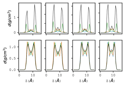
Figure 2: The density profile of interlayer cation water molecules of a Fluorohectorite clay as a function of $z$ coordinate, at various temperature values. The temperature values start from left and the top figure is for ions and below is water.  Colors: green-KFht , Orange-NaFht, black - CsFht and blue-LiFht for at T=350 K.

A detailed analysis requires the radial distribution function (RDF) of interlayer cation atoms with respect to reference oxygen atoms of water, which are shown in Figs. 3-6, with red color. For K and Cs-Fluorohectorite, the 1^st neighbouring peak has $g(r)$ peak intensity values of 7.64 at T=293 K; 7.30 at T=300 K; 7.22 at T=323 K; 7.33 at T=350 K; 5.47 at T=300 K; 5,46 at T=300 K; 5.45 at T=323 K; and 5.38 at T=350 K. However, for Li and Na-Fluorohectorite, the 1^st neighbouring peak has $g(r)$ peak intensity values of 25.13 at T=293 K; 24.50 at T=300 K; 23.92 at T=323 K; 22.45 at T=350 K; 19.76 at T=293 K, 19.55 at T=300 K; 18.47 at T=323 K; and 17.24 at T=350 K. This result simply shows that the peak intensity change owing to the presence of different interlayer cations. In addition to this, comparing with the hydration shell around K⁺¹ and Cs⁺¹ cations, we found that the $1^{st}$ neighbour cation oxygen are assembled more densely than compared to those in the case of Li⁺¹ and Na⁺¹ cations, which is the reason why the $1^{st}$ neighbour peak of K and Cs-Fluorohectorite are less than that of Li and Na-fluorohectorite. It is well known that the interaction of the clay cation with their environment depends on non-bonding electrostatics and van der Waals potentials. As shown in the Figures discussed above, the RDFs between the cation and the clay tetrahedral oxygen atom of the hydrated clay clearly show the structure. Similarly, the RDF of interlayer cation with reference to basal oxygen of clay is also plotted and represented by black color in all the Figs. 3-6. We can see the exclusion region up to a certain distance, where the probability of finding the particle with respect to the reference particle is zero. As we go to right side of each point, the height of the peaks keep on decreasing. This means that the distance between the reference atom and atom under the study increases. The correlation between them decreases and eventually there won’t be any long range correlation for a large value of $r$, i.e., $g(r)\leavevmode\nobreak\ {\rightarrow}\leavevmode\nobreak\ 1$ [23]. The exclusion region for cation-OW and cation-OB correlation pair are provided in Table 1 at all temperature.

Table 1: The exclusion region of each correlation pair in Å for different temperatures.

Correlation pair	Temperature [K]
	293 K	300 K	323 K	350 K
Cs-OW	0.267	0.269	0.272	0.268
Cs-OB	0.278	0.278	0.279	0.278
K-OW	0.249	0.250	0.250	0.250
K-OB	0.259	0.260	0.260	0.260
Li-OW	0.189	0.191	0.197	0.196
Li-OB	0.206	0.197	0.197	0.196
Na-OW	0.214	0.215	0.213	0.209
Na-OB	0.216	0.220	0.220	0.216

The coordination number of interlayer cations is the number of molecule of water and basal oxygen of the clay in the immediate neighbour of the cations. It depends on the distance between the water molecule as well as the basal oxygen of clay and cations. In Tables 2 $\&$ 3, the coordination number of each correlation pair is presented.

Table 2: The coordination number of different clays with different temperature.

T [K]	LiFht			NaFht
	Li-OW	Li-OB	Li-HW	Na-OW	Na-OB	Na-HW
293	1.93	1.23	1.67	1.85	1.24	1.65
300	1.90	1.22	1.64	1.85	1.24	1.64
323	1.92	1.23	1.67	1.83	1.24	1.63
350	1.90	1.24	1.65	1.79	1.25	1.60

Table 3: The coordination number of different clays with different temperature.

T [K]	KFht			CsFht
	K-OW	K-OB	K-HW	Cs-OW	Cs-OB	Cs-HW
293	1.54	1.24	1.44	1.49	1.32	1.42
300	1.54	1.34	1.45	1.49	1.32	1.42
323	1.54	1.34	1.45	1.49	1.32	1.42
350	1.55	1.30	1.46	1.50	1.32	1.42

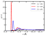
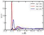
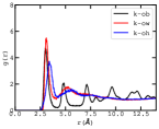
Figure 3: The RDF analysis of $g(r)$ at T=293 K. Colors: red for cation-OW, black for cation-OB, and blue for cation-HW. Cations from left to right are Li⁺, Na⁺, K⁺, and Cs⁺, respectively. For the interpretations of the references to color in this plot legend, the reader is referred to the web-version.

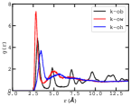
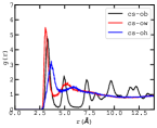
Figure 4: The RDF analysis of $g(r)$ at T=300 K. Colors: red for cation-OW, black for cation-OB, and blue for cation-HW. Cations from left to right are Li⁺, Na⁺, K⁺, and Cs⁺, respectively. For the interpretations of the references to color in this plot legend, the reader is referred to the web-version.

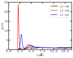
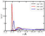
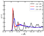
Figure 5: The RDF analysis of $g(r)$ at T=323 K. Colors: red for cation-OW, black for cation-OB, and blue for cation-HW. Cations from left to right are Li⁺, Na⁺, K⁺, and Cs⁺, respectively. For the interpretations of the references to color in this plot legend, the reader is referred to the web-version.

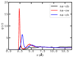
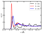
Figure 6: The RDF analysis of $g(r)$ at T=350 K. Colors: red for cation-OW, black for cation-OB, and blue for cation-HW. Cations from left to right are Li⁺, Na⁺, K⁺, and Cs⁺, respectively. For the interpretations of the references to color in this plot legend, the reader is referred to the web-version.

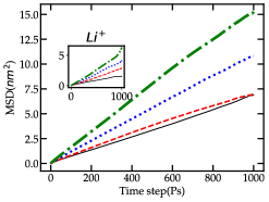
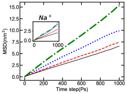
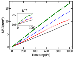
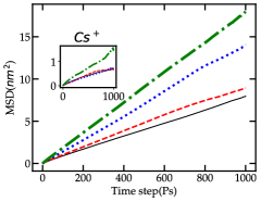
Figure 7: The mean square displacement graph as a function of time step ($ps$) of interlayer cations $\&$ water. Colors: black for T=393 K,  red for T=300 K, blue for T=323 K and green for T=350 K.

The Figure 7 show the mean square displacement (MSD) plots of interlayer cations (Cs⁺, K⁺, Li⁺, Na⁺), and H$\rm{}_{2}O$ molecule in CsFht, KFht, LiFht and NaFht, at different temperatures ranging from 293 K to 350 K, respectively. The corresponding simulated result of self diffusion coefficients in 3D and 2D are shown in Tables 4 $\&$ 5, respectively. It is clearly observed that when temperature increases, the generated velocities of the ions and water molecules also increase and the density of the system decreases. This provides more space for the molecule to execute random walk. Due to this, the mean square displacement increases. From Einstein’s relation in Eq. (6), as the mean square displacement increases, the self diffusion coefficient also increases.
Comparing the simulated results of the diffusion coefficients of water with the experiment and other simulation values, at T=300 K, water molecule within the bilayer has self diffusion coefficient of $[1.0-1.5]\leavevmode\nobreak\ {\times}\leavevmode\nobreak\ 10^{-5}{cm^{2}}s^{-1}$. According to a literature [24], it is varies from $[1.96-2.33]\leavevmode\nobreak\ {\times}\leavevmode\nobreak\ 10^{-6}{cm^{2}}s^{-1}$. Water diffusion coefficients in a synthetic hectorite clay is investigated by a literature [25], to be $[4.6\leavevmode\nobreak\ {\pm}\leavevmode\nobreak\ 0.3]\leavevmode\nobreak\ {\times}\leavevmode\nobreak\ 10^{-6}{cm^{2}}s^{-1}$ (NSE) and $[4.3\leavevmode\nobreak\ {\pm}\leavevmode\nobreak\ 0.1]\leavevmode\nobreak\ {\times}\leavevmode\nobreak\ 10^{-6}{cm^{2}}s^{-1}$ (TOF). But according to the recent measurement of (TOF) on bihydrated vermiculite, the results are slightly deviated from the above values, i.e., it is $2.7\leavevmode\nobreak\ {\times}\leavevmode\nobreak\ 10^{-5}{cm^{2}}s^{-1}$ [26]. The diffusion coefficient of water in sodium vermicutite (Na-Ver) and cesium vermicutite (Cs-Ver) is $1.6\leavevmode\nobreak\ {\times}\leavevmode\nobreak\ 10^{-6}{cm^{2}}s^{-1}$ and $1.8\leavevmode\nobreak\ {\times}\leavevmode\nobreak\ 10^{-6}{cm^{2}}s^{-1}$, respectively. From bihydrated (Na⁺, Cs⁺) montmorilonite clay, the result is $[1.2-1.5]\leavevmode\nobreak\ {\times}\leavevmode\nobreak\ 10^{-5}{cm^{2}}s^{-1}$ [27, 28]. Our result of diffusion coefficient of water in Na-Fht and Cs-Fht at 300 K is $[1.20\leavevmode\nobreak\ {\pm}\leavevmode\nobreak\ 0.06]\leavevmode\nobreak\ {\times}\leavevmode\nobreak\ 10^{-5}{cm^{2}}s^{-1}$ and $[1.52\leavevmode\nobreak\ {\pm}\leavevmode\nobreak\ 0.18]\leavevmode\nobreak\ {\times}\leavevmode\nobreak\ 10^{-5}{cm^{2}}s^{-1}$, respectively.
The actual diffusion coefficient of water is $2.27\leavevmode\nobreak\ {\times}\leavevmode\nobreak\ 10^{-5}{cm^{2}}s^{-1}$. These values of diffusion coefficients are higher than half of the bulk value for water, which is $D_{exp}^{bulk-{H_{2}}O}=2.3\leavevmode\nobreak\ {\times}\leavevmode\nobreak\ 10^{-5}{cm^{2}}s^{-1}$. This is true for three types of clay studied (hectorite, montmorillonite, vermiculite) and both mono and divalent counterions [29, 30, 25]. In Table 4, the diffusion coefficient of interlayer cation of synthetic fluorohectorite clay is presented. From this, one can see that the diffusivity of Na⁺ $>$ Li⁺ $>$ K⁺ $>$ Cs⁺ at T=293K, Na⁺ $>$ Li⁺ $>$ K⁺ $>$ Cs⁺ at T=300 K, Li⁺ $>$ Na⁺ $>$ K⁺ $>$ Cs⁺ at T=323 K, and Li⁺ $>$ Na⁺ $>$ K⁺ $>$ Cs⁺ at T=350 K. When the temperature is 323 K and 350 K, the diffusivity of Na⁺ ion is less than Li⁺ ion. This implies that the reactivity of sodium ion is also higher than that of lithium ion whenever there is increase in temperature. Thus, our choice of interlayer cation also affects the diffusivity of water. Our simulated result is compared with another natural smectite clay called montmorilonite and natural hectorite clay. For montmorilonite clays, using monovalent counterions called (Na⁺, Cs⁺) in bihydrated system, the self diffusion coefficient is $D_{sim}^{ions}=3.7-10.0\leavevmode\nobreak\ {\times}\ 10^{-6}{cm^{2}}s^{-1}$ [27, 28].
In the confining environment of nanochannels, the lateral self diffusion coefficients for motion parallel to the clay sheets are more relevant and necessary. Due to this, we have calculated the lateral diffusion coefficient of both interlayer cation and water for all temperature values and types of Fluorohectorite clay. The result is presented in Table 5. According to a literature [25], the lateral diffusion coefficient of water in Na-montmorilonite is $D_{xy}=[7.7\leavevmode\nobreak\ {\pm}\leavevmode\nobreak\ 1.0]\leavevmode\nobreak\ {\times}\ 10^{-6}{cm^{2}}s^{-1}$ (NSE). Generally, in all cases, the self diffusion coefficient of both cations and water depend on temperature. As the temperature increases, the diffusion coefficients also increase. Figure 7 shows the of MSD of ions and water at different temperatures. The main factor for the retarding diffusion coefficient of interlayer water and cation is the electrostatic interaction between water and cation with the clay sheet.

Table 4: Region-Specific Diffusivity (${\times}10^{-5}cm^{2}s^{-1}$) of interlayer cation and water through our Model Synthetic Clay.

T(K)	$D_{Cs}^{CsFht}$	$D_{H_{2}O}^{CsFht}$	$D_{K}^{KFht}$	$D_{H_{2}O}^{KFht}$	$D_{Li}^{LiFht}$	$D_{H_{2}O}^{LiFht}$	$D_{Na}^{NaFht}$	$D_{H_{2}O}^{NaFht}$
293	0.11 $\pm$ 0.05	1.28 $\pm$  0.01	0.19 $\pm$ 0.01	1.55 $\pm$  0.08	0.26 $\pm$ 0.01	1.12 $\pm$  0.09	0.34 $\pm$ 0.01	1.06 $\pm$  0.02
300	0.13 $\pm$ 0.09	1.52 $\pm$  0.18	0.29 $\pm$ 0.06	1.88 $\pm$  0.07	0.48 $\pm$ 0.06	1.17 $\pm$  0.18	0.49 $\pm$ 0.07	1.20 $\pm$  0.06
323	0.11 $\pm$ 0.01	2.42 $\pm$  0.09	0.29 $\pm$ 0.15	2.33 $\pm$  0.19	0.69 $\pm$ 0.03	1.82 $\pm$  0.04	0.68 $\pm$ 0.18	1.67 $\pm$  0.06
350	0.22 $\pm$ 0.01	2.97 $\pm$  0.08	0.43 $\pm$ 0.23	2.87 $\pm$  0.17	0.91 $\pm$ 0.07	2.59 $\pm$  0.22	0.68 $\pm$ 0.08	2.45 $\pm$  0.10

Table 5: Region-Specific Lateral Diffusivity (${\times}10^{-5}cm^{2}s^{-1}$) of interlayer cations and water through our Model Synthetic Clay.

T(K)	$D_{||}^{Cs}$	$D_{||(H_{2}O)}^{CsFht}$	$D_{||}^{K}$	$D_{||(H_{2}O)}^{KFht}$	$D_{||}^{Li}$	$D_{||(H_{2}O)}^{LiFht}$	$D_{||}^{Na}$	$D_{||(H_{2}O)}^{NaFht}$
293	0.15 $\pm$  0.07	1.92 $\pm$ 0.02	0.27 $\pm$ 0.01	2.32 $\pm$ 0.13	0.39 $\pm$ 0.02	1.68 $\pm$ 0.14	0.50 $\pm$  0.01	1.86 $\pm$  0.03
300	0.17 $\pm$ 0.12	2.28 $\pm$ 0.26	0.42 $\pm$ 0.10	2.83 $\pm$ 0.11	0.71 $\pm$ 0.08	1.75 $\pm$ 0.27	0.73 $\pm$ 0.12	1.80 $\pm$  0.103
323	0.15 $\pm$ 0.02	2.28 $\pm$ 0.26	0.42 $\pm$ 0.18	3.49 $\pm$ 0.29	1.03 $\pm$ 0.05	2.72 $\pm$ 0.06	1.01 $\pm$ 0.28	2.49 $\pm$  0.09
350	0.31 $\pm$ 0.03	4.46 $\pm$ 0.1	0.64 $\pm$ 0.33	4.30 $\pm$ 0.26	01.34 $\pm$ 0.10	3.88 $\pm$ 0.33	1.01 $\pm$  0.12	3.68 $\pm$  0.16

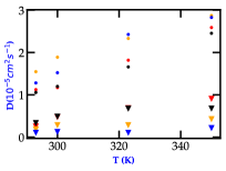
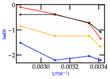
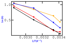
Figure 8: The (a) Diffusion coefficient vs temperature graph and (b) The natural logarithm of 3D diffusion coefficient vs inverse temperature graph of interlayer molecules of Li, Na, K and Cs-Fht clays. (c) The natural logarithm of 3D diffusion coefficient vs inverse temperature graph of water molecule. Colors: red-LiFht, black-NaFht, orange-KFht $\&$ black-CsFht.

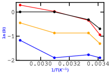
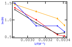
Figure 9: (a) Lateral diffusion coefficient vs temperature graph and (b) The natural logarithm of 2D diffusion coefficient vs inverse temperature graph of interlayer molecules of Li, Na, K and Cs-Fht clays. (c) The natural logarithm of 2D diffusion coefficient vs inverse temperature graph of water molecule. Colors: red-LiFht, black-NaFht, orange-KFht $\&$ black-CsFht.

Fig. 8(b) $\&$ (c) $\&$ Fig. 9(b) $\&$ (c) shows the Arrhenius plot of the diffusion coefficient plot of interlayer molecules. We may determine the pre-exponential factor by extrapolating the graph to zero. The activation energy of water calculated from the simulation was 13.05 $\frac{kJ}{mol}$, 12.46 $\frac{kJ}{mol}$, 8.68 $\frac{kJ}{mol}$, $\&$ 12.07 $\frac{kJ}{mol}$ in Li, Na, K, and Cs-Fht, respectively, and the activation energy of Li, Na, K, and Cs was 16.62 $\frac{kJ}{mol}$, 9.55 $\frac{kJ}{mol}$, 9.94 $\frac{kJ}{mol}$, $\&$ 8.52 $\frac{kJ}{mol}$, respectively, in 3D motion of molecules.

4 Conclusion

The transport characteristics of cations and water molecules in bihydrated Li, Na, K, and Cs-Fht clays were studied using MD simulations. Na⁺ and Li⁺ ions exhibit a qualitative difference from K⁺ and Cs⁺ ions, according to trajectory maps of the cations  on the simulation time scale 1000 $ps$. The former exhibits significant diffusion motion, including hopping events, whereas, the later exhibits more constrained motion, probably due to its stronger interaction with the stiff clay surface than with the mobile water molecules.
The reason looks to be due to more K⁺ $\&$ Cs⁺ ions than Na⁺ $\&$ Li⁺ ions adsorbing on the clay surface, according to density profiles. Consequently, it can be inferred that K⁺ $\&$ Cs⁺ ions screen the negatively charged surface more efficiently than Na⁺ $\&$ Li⁺ ions. The self-diffusion coefficient’s measurement reveal that the values rise as the temperature rises. Diffusion coefficients for bilayer states are typically in the order of $10^{-5}cm^{2}s^{-1}$ in most neutron scattering experiments (mostly TOF) on natural clays, like montmorillonite, hectorite, or vermiculite. In the synthetic hectorite clay, it is reasonable to expect that the liquid phase is evenly distributed throughout various interlayers and may even be better ordered. As a result, water would move more slowly in synthetic hectorite than in other systems. But, the outcomes for Na, Li, K, and Cs-Fht are satisfactorily consistent with other simulation and experiment literatures.

This shows that the clay interlayer spacing is a crucial path-way for the transportation of ions and water, and it supports the accuracy of the diffusion coefficients investigated by this work.

The present study and its future extensions, for example to the case of the different water model in the clay, opens the possibility to use simulations to study detailed processes occurring in clays which can not be seen experimentally, to analyse data mixing by several dynamics such as rotation and vibrations, and to model accurately more and more complex systems approaching the real natural clays.

Disclosure statement

The authors declare that there is no conflict of interest.

References

References

-
[1]
L. Michels, J. O. Fossum, Z. Rozynek, H. Hemmen, K. Rustenberg, P. A. Sobas,
G. N. Kalantzopoulos, K. D. Knudsen, M. Janek, T. S. Plivelic, et al.,
Intercalation and retention of
carbon dioxide in a smectite clay promoted by interlayer cations, Scientific
reports 5 (2015) 8775.
URL https://doi.org/10.1038/srep08775 -
[2]
P. Giesting, S. Guggenheim, A. F. Koster van Groos, A. Busch,
Interaction of carbon
dioxide with Na-exchanged montmorillonite at pressures to
640 bars: Implications for CO2 sequestration, International Journal
of Greenhouse Gas Control 8 (2012) 73–81.
URL https://doi.org/10.1016/j.ijggc.2012.01.011 -
[3]
E. Galán, P. Aparicio,
Experimental study on the
role of clays as sealing materials in the geological storage of carbon
dioxide, Applied Clay Science 87 (2014) 22–27.
URL https://doi.org/10.1016/j.clay.2013.11.013 -
[4]
A. Azzouz, E. Assaad, A.-V. Ursu, T. Sajin, D. Nistor, R. Roy,
Carbon dioxide retention
over montmorillonite–dendrimer materials, Applied Clay Science 48 (2010)
133–137.
URL https://doi.org/10.1016/j.clay.2009.11.021 -
[5]
L. Michels, C. Da Fonseca, Y. Méheust, M. Altoe, E. Dos Santos, G. Grassi,
R. Droppa Jr, K. D. Knudsen, L. P. Cavalcanti, K. W. B. Hunvik, et al.,
The Impact of Thermal
History on Water Adsorption in a Synthetic Nanolayered Silicate with
Intercalated Li+ or Na+, The Journal of Physical Chemistry
C 124 (2020) 24690–24703.
URL https://doi.org/10.1021/acs.jpcc.0c05847 -
[6]
S. R. Larsen, L. Michels, É. C. dos Santos, M. C. Berg, W. P. Gates, L. P.
Aldridge, T. Seydel, J. Ollivier, M. T. Telling, J. O. Fossum, et al.,
Physicochemical
characterisation of fluorohectorite: Water dynamics and nanocarrier
properties, Microporous and Mesoporous Materials 306 (2020) 110512.
URL https://doi.org/10.1016/j.micromeso.2020.110512 -
[7]
M. A. S. Altoé, L. Michels, E. dos Santos, R. Droppa Jr, G. Grassi,
L. Ribeiro, K. Knudsen, H. N. Bordallo, J. O. Fossum, G. J. da Silva,
Continuous water
adsorption states promoted by Ni2+ confined in a synthetic
smectite, Applied Clay Science 123 (2016) 83–91.
URL https://doi.org/10.1016/j.clay.2016.01.012 -
[8]
E. Dos Santos, Z. Rozynek, E. L. Hansen, R. Hartmann-Petersen, R. Klitgaard,
A. Løbner-Olesen, L. Michels, A. Mikkelsen, T. S. Plivelic, H. Bordallo,
et al., Ciprofloxacin intercalated
in fluorohectorite clay: identical pure drug activity and toxicity with
higher adsorption and controlled release rate, RSC advances 7 (2022) 26537.
URL https://doi.org/10.1039/C7RA01384A -
[9]
D. Hernández, L. Lazo, L. Valdés, L. de Ménorval, Z. Rozynek,
A. Rivera, Synthetic clay
mineral as nanocarrier of sulfamethoxazole and trimethoprim, Applied Clay
Science 161 (2018) 395.
URL https://doi.org/10.1016/j.clay.2018.03.016 -
[10]
E. Dos Santos, W. Gates, L. Michels, F. Juranyi, A. Mikkelsen, G. da Silva,
J. Fossum, H. Bordallo,
The pH influence on the
intercalation of the bioactive agent ciprofloxacin in fluorohectorite,
Applied Clay Science 166 (2018) 288.
URL https://doi.org/10.1016/j.clay.2018.09.029 -
[11]
C.-H. Zhou, D. Tong, X. Li,
Synthetic Hectorite:
Preparation, Pillaring and Applications in Catalysis, Springer New York,
New York, NY, 2010, pp. 67–97.
URL https://doi.org/10.1007/978-1-4419-6670-4_4 -
[12]
D. Zhang, C.-H. Zhou, C.-X. Lin, D.-S. Tong, W.-H. Yu,
Synthesis of clay
minerals, Applied Clay Science 50 (2010) 1–11.
URL https://doi.org/10.1016/j.clay.2010.06.019 - [13] C. Zhou, Z. Du, X. Li, C. Lu, Z. Ge, Structure development of hectorite in hydrothermal crystallization synthesis process, Chinese Journal of Inorganic Chemistry 21 (2005) 1327.
-
[14]
F. Bergaya, G. Lagaly,
Handbook of Clay
Science, Developments in Clay Science, Elsevier Science, 2013.
URL https://books.google.com.et/books?id=35z6jwEACAAJ - [15] J. Breu, W. Seidl, A. Stoll, Disorder in smectites in dependence of the interlayer cation (2003).
- [16] M. Allen, D. Tildesley, Computer simulation of liquids, Oxford University press, UK, 1989.
-
[17]
E. M. Myshakin, W. A. Saidi, V. N. Romanov, R. T. Cygan, K. D. Jordan,
Molecular dynamics simulations of
carbon dioxide intercalation in hydrated Na-montmorillonite, The Journal of
Physical Chemistry C 117 (2013) 11028–11039.
URL https://doi.org/10.1021/jp312589s -
[18]
H. J. C. Berendsen, J. R. Grigera, T. P. Straatsma,
The missing term in effective pair
potentials, The Journal of Physical Chemistry 91 (1987) 6269–6271.
URL https://doi.org/10.1021/j100308a038 - [19] P. M. Chaikin, T. C. Lubensky, T. A. Witten, Principles of condensed matter physics, Vol. 10, Cambridge university press Cambridge, 1995. doi:10.1557/mrs2001.250.
- [20] A. C. F. Ribeiro, O. Ortona, S. M. N. Simões, C. I. A. V. Santos, P. M. R. A. Prazeres, A. J. M. Valente, V. M. M. Lobo, H. D. Burrows, Binary mutual diffusion coefficients of aqueous solutions of sucrose, lactose, glucose, and fructose in the temperature range from (298.15 to 328.15) k, Journal of Chemical & Engineering Data 51 (2006) 1836–1840.
-
[21]
I. Poudyal, N. P. Adhikari,