[0]Doctoral School of Exact and Natural Sciences, Jagiellonian University, ul. Łojasiewicza 11, 30-348 Kraków, Poland \affil[1]Faculty of Physics, Astronomy and Applied Computer Science, Jagiellonian University, ul. Łojasiewicza 11, 30-348 Kraków, Poland \affil[2]Centrum Fizyki Teoretycznej PAN, Al. Lotników 32/46, 02-668 Warszawa, Poland \affil[3]National Quantum Information Center (KCIK), University of Gdańsk, Poland \affil[4]Institute of Theoretical Physics, University of Tübingen, Auf der Morgenstelle 14, 72076 Tübingen, Germany
Minimal-noise estimation of noncommuting rotations of a spin
Abstract
We propose an analogue of interferometry to measure rotation of a spin by using two-spin squeezed states. Attainability of the Heisenberg limit for the estimation of the rotation angle is demonstrated for maximal squeezing. For a specific squeezing direction and strength an advantage in sensitivity for all equatorial rotation axes (and hence non-commuting rotations) over the classical bound is shown in terms of quadratic scaling of the single-parameter quantum Fisher information for the corresponding rotation angles. Our results provide a method for measuring magnetic fields in any direction in the --plane with the same optimized initial state.
1 Introduction
For more than a century light interferometry has proven to be an invaluable tool for the progress of physics. Recent developments of interferometry making use of squeezed states of light are applied at the cutting edge of experimental physics of gravitational waves and axions [1, 2, 3, 4].
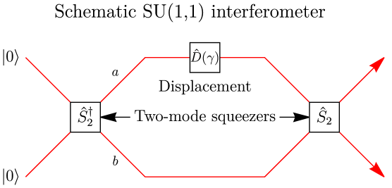
In a seminal work Yurke, McCall and Klauder [5] considered a Mach-Zehnder interferometer with the beam-splitters replaced by non-linear crystals as four-wave mixers, pumped with a common strong laser beam. While in the standard Mach-Zehnder interferometer the variance of any unbiased estimation of the phase shift in one arm relative to the other scales with the number of photons as the inverse square root, , the so-called standard quantum limit, they demonstrated that the modified interferometer generates a transformation of the annihilation and creation operators of the two modes and achieves the scaling , now known as the Heisenberg limit. In a recent reinterpretation, Caves [6] argued that such a interferometer can be understood as a “displacement detector”: On an initial coherent state it generates a sequence of squeeze – displace – unsqueeze operations, where the displacement refers to the displacement of the label of the coherent state in the complex plane. The net result of the three operations is a noiseless amplification of the displacement.
Using two oscillators, the added noise in the displacement of both quadratures can be made arbitrarily small [7]. The noiseless amplification of displacements of two non-commuting quadratures should be contrasted with the fact that two non-commuting quadratures themselves cannot be measured simultaneously with arbitrarily small statistical error, as this would violate Heisenberg’s uncertainty relation. Nor is it possible to amplify even a single quadrature without adding noise (see e.g. [8], p.220 ff), such that the quantumness of an amplified signal is normally quickly lost in the amplification process. Measuring the displacement of both quadratures is achieved by using two modes, one for each quadrature, whose relative coordinate and total momentum (in oscillator parlance) do commute, hence allowing arbitrarily small statistical error for both displacements.
In the micro-wave domain, noiseless amplification of small signals plays an important role and has been boosted by the tremendous technological progreess in the context of quantum computing based on super-conducting qubits [9, 10, 11, 12], as well as with nano-mechanical oscillators [13]. Recently, noiseless microwave amplification has even been proposed for speeding-up the search for axions [14, 15].
Here we transfer the SU(1,1) protocol to spin-systems. The displacement of a coherent state of a harmonic oscillator has its analogue in the rotation of spin-coherent states, which, in the case of physical spins, can be generated with applied magnetic fields (whereas pseudo-spins- representing generic -level systems can be rotated by driving transitions between these levels). Our investigations have therefore direct application for magnetometry, where one wants to measure magnetic fields in different directions. We follow the interpretation of Caves of SU(1,1) interferometry and transplant it to the realm of spins by employing the spin squeezed states introduced by Kitagawa and Ueda in [16] and their extension to 2-spins squeezed states [17, 18]. Schemes utilising squeezing of spin states have been recently demonstrated experimentally to yield significant advantages over the classical limits of sensitivity in the context of Bose-Einstein condensates [19, 20], ultracold dipolar molecules [21], spectroscopy on beryllium atoms [22], rotosensors [23], programmable quantum sensors [24], and others [25, 26, 27].
We demonstrate that a squeeze-rotate-unsqueeze (SRU) protocol for a single spin as well as for a two-spin system is able to achieve the Heisenberg scaling of the single-parameter quantum Fisher information (QFI) for rotation estimation, in the size of the displaced system, for particular equatorial axes of rotation. Moreover, for a particular value of squeezing we demonstrate scaling of the single parameter for any equatorial rotation axes, hence for non-commuting rotations. Both results are achieved using oversqueezing, thus demonstrating its usefulness for the quantum metrological applications. Finally, we consider the problem of estimation of the rotation axis, as contrasted with the estimation of the rotation angle around a known axis. Therein we show that the quantum Cramer-Rao bounds are attainable given a proper choice of the parameter values for which the estimation is carried out.
A word is in order about the possility to estimate the rotation angles for non-commuting rotations (with rotation axes in the -plane) “simultaneously” with Heisenberg-limited sensitivity. In the framework of multi-parameter quantum metrology, with “simultaneously” it is commonly understood that there exists a measurement that saturates the matrix-valued quantum Cramér-Rao bound for the co-variance matrix of the estimators. It requires the commutation on average of the corresponding symmetric logarithmic derivatives (SLDs) of the density matrix. As we shall see, this is, for the problem at hand, only possible for few, specific combinations of parameters. Rather, what we show generically, is that the values of the single-parameter QFI for different rotation angles about rotation axes in the -plane that lead to non-commuting rotations all scale up to exponentially small terms in probe spin . This is exactly in the same spirit as noiseless amplification of both quadratures of a single mode of an electro-magnetic field. To illustrate this, we provide in Appendix A a general analysis of the SU(1,1) interferometry and the SDU protocol using the lens of QFI. In case of a single-mode SDU protocol it proves that only one direction of the displacement at a time can be estimated with an enhanced sensitivity. For a two-mode protocol serving as a basis for the SU(1,1) interferometry we show that the QFI matrix is proportional to the identity. This allows estimation of displacements in any direction with the same enhanced sensitivity. Nevertheless, the symmetric logarithmic derivatives do not commute, which prevents any multivariate estimation scheme to saturate the multi-parameter quantum Cramer-Rao bound for simultaneous estimation of the displacement of the two quadratures.
2 Setting the Scene
2.1 Group-theoretic approach to interferometry
Consider a standard Mach-Zehnder interferometer consisting of two arms and describe the state of light in its two arms by annihilation operators and respectively, together with their standard commutation relations and . It is then easily verified that operators of the form
| (1) |
together with the number operator provide an SU(2) representation with the Casimir operator given by . Making use of the isomorphism and the resulting geometric interpretation, Yurke et al. have shown that the standard limit of fluctuation of phase estimation is given as with the average number of photons in a coherent state used in the interferometer [5].
In a similar manner they demonstrated that a four-wave mixer can be identified with a representation of a non-compact group SU(1,1) given by
| (2) |
which provide generators for a set of squeezing operators. It has been demonstrated that this kind of active optical elements, when incorporated into the structure of Mach-Zehnder interferometer, allows for measurement of a phase shift with fluctuations on the order of .
Caves in his reinterpretation [6] presents a useful perspective on the action of SU(1,1) interferometer as a composition of three operations – squeezing, displacement, and unsqueezing (SDU in short), defined for a single mode as
| (3) |
where the squeezing operators are defined as . The displacement operator reads, , and is a vacuum state defined as a coherent state of light with the average of both quadratures equal to . Similarly, a two-mode protocol is defined by a composition
| (4) |
with the two-mode squeezing operators , and single mode displacement .
Caves demonstrated that for a single mode it is possible to achieve a resolution of in an -fold repetition of the protocol, at the cost of decreasing the complementary resolution, . Furthermore, for the two-mode protocol he furthermore demonstrated the possibility of estimation of the full displacement with enhanced resolution, . The possibility of achieving such an advantage for two non-commuting observables can be understood by noting that they can be reconstructed from measurements of displacements of two Bell variables and , for which the squeezing occurs, while the other two variables are unsqueezed.
2.2 Spin Coherent and Squeezed States
Spin coherent states (SCS), first introduced in 1971 by Radcliffe [28] by analogy to the coherent states of light and later analysed in further details by Arecchi et al. and Holtz and Hanus [29, 30], can be understood most easily in terms of a collection of spin particles, all in an eigenstate of the operator, , with the positive eigenvalue, . By projecting the state of such a collection onto the -dimensional subspace spanned by the symmetric states one arrives at a well known expression,
| (5) |
where the basis states are defined as eigenstates of spin operator , namely , defining the basis for states constituting a -dimensional representation of the SU(2) group. The group-theoretic approach to the SCS and an extensive review can be found in [31].
In a seminal work [16] Kitagawa and Ueda reimagined what it means for a spin state to be squeezed by understanding that one should consider the squeezing in directions perpendicular to the main axis of a SCS. The authors proposed two squeezing hamiltonians,
| (6) |
also referred to in the literature as one-axis squeezing (OAT) and two-axis counter-twisting (TACT), respectively. By evolving the SCS with each of them one gets one- and two-axis squeezed spin states, respectively. In this work we will be particularly interested in the former, which defines the squeezed states
| (7) | ||||
In particular, we will be interested in squeezing the SCS along the axis, therefore we introduce the notation
| (8) |
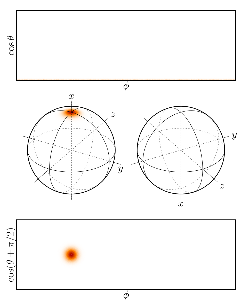
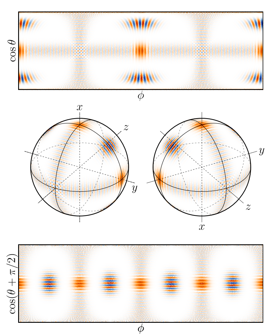
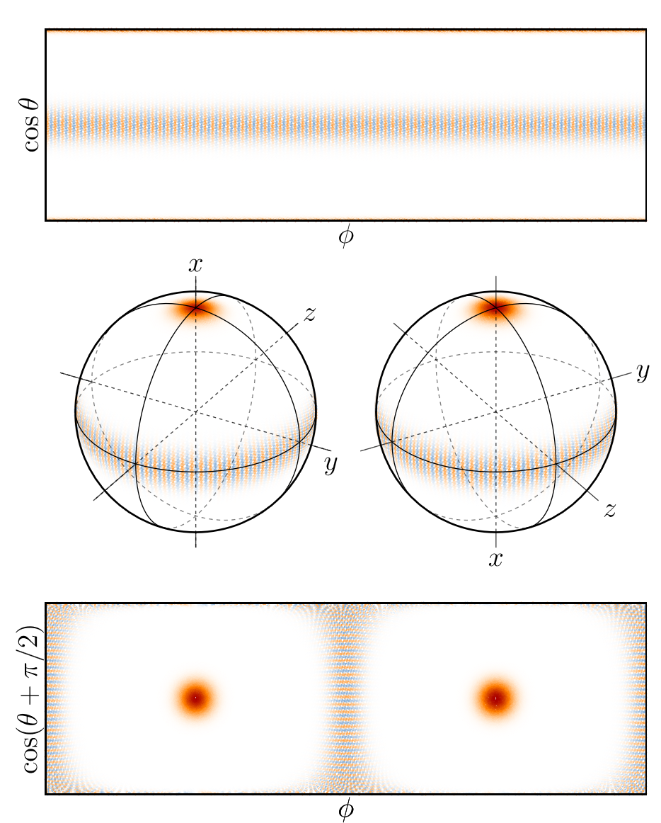
We note that and . Note that squeezed spin states can be oversqueezed, unlike for the squeezed states of light, which has been emphasized in the original work of Kitagawa and Ueda. In Fig 2 we present three examples of squeezed spin states most important in this work, ranging from SCS with to the maximum squeezing of . For the visualization we go to the spherical Wigner function, as defined in [32], later analysed in [33] and [34] in the context of negativity of the spherical Wigner function [35].

A two-spin counterpart for one-spin squeezing has already been studied in experimental works [17, 18], whereas the two-spin two-axis squeezing has been studied only recently in [36], where its chaotic behaviour has been demonstrated. Therefore we restrict our attention in this work to the two-spin one-axis squeezed states defined as
| (9) |
2.3 Quantum Fisher Information and Hamiltonian Estimation
As a proxy for the sensitivity of rotation estimation we will use the quantum Fisher information in connection to the quantum Cramér-Rao bound, defined in the following theorem [37, 38, 39, 40, 41].
Theorem 1.
Consider a family of states depending on a scalar parameter . The variance of any locally unbiased estimator
is bounded from below by the inverse of the Quantum Fisher Information
| (10) |
with the quantum Fisher information (QFI).
The QFI can be defined in terms of the symmetric logarithmic derivative (SLD) ,
| (11) |
where the SLD itself is defined implicitly by
For the purpose of this work, however, we are mostly concerned with the closed form of QFI for pure states. Given that one finds that the expression for QFI reduces to
| (12) |
Similarly, the elements of SLD can be expressed in a closed form in terms of the eigenbasis of as
| (13) |
and the optimal measurement saturating the bound on the variance given by QFI can be given in terms of projectors on the eigenvectors of the SLD. If is a pure state, the SLD simplifes to [42].
To illustrate the classical limit of the QFI, it is a rudimentary task to calculate this quantity for the rotation angle ,
| (14) |
This implies that QFI takes the form,
| (15) |
which shows linear scaling with the number of the systems , often referred to as the “classical limit” or “Standard Quantum Limit” (SQL), in agreement with the fact that and the state is considered the most classical state of a spin system [29, 43]. In the remainder of this paper we demonstrate a protocol that allows quadratic scaling with , thus the quantum counterpart of the classical limit.
One can generalize the quantum Cramér-Rao bound to multi-parameter estimation. In such a case one considers the covariance matrix of an estimator , defined for a vector-valued parameter . This leads to the bound [44, 45]
| (16) |
where the quantum Fisher information matrix is defined elementwise as
| (17) |
where denotes the anti-commutator. In contrast to the single parameter quantum Cramér-Rao bound, the bound (16) can usually not be saturated. A bound that can be up to a factor two tighter [46] and that can be saturated asymptotically in the limit of infinitely many samples was introduced by Holevo [47], but it is, in general, more difficult to evaluate than the quantum Cramér-Rao bound. If the SLD operators for different parameters commute on average, , then this Holevo-Cramér-Rao bound coincides with the quantum Cramér-Rao bound, such that also the latter can be saturated asymptotically [48, 49, 50, 46]. In particular, for pure states, , the average commutation relation is given by
| (18) |
3 Results
3.1 Selected axes for single-spin maximal squeezing
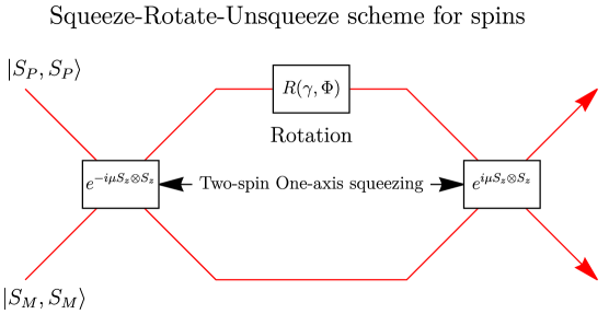
Following the steps of SU(1,1) interferometry in the formulation by Caves, we translate the squeeze-displace-unsqueeze procedure into its spin equivalent, squeeze-rotate-unsqueeze (SRU), closely related to the already successful experimental delta-kick squeezing (DKS) protocol [20]. We begin the extension of the interferometric scheme to spins by considering a toy example of a single spin. First we define the SRU protocol acting on a SCS along the axis, which serves as an equivalent for the bosonic vacuum ,
| (19) |
with . In particular, such a rotation could be induced by interaction with the magnetic field via standard Hamiltonian . with the magnetic moment proportional to the spin vector, . In such case the angle could be used to estimate either the time of interaction for constant field or the magnitude of field for a fixed direction of field and interaction time. Similar unitary operators were used in investigation of the phenomenon of quantum chaos in the model of the quantized kicked top [51, 52, 53, 54]. As a further simplification we limit the axis around which the spin can rotate to . If we consider the case of the maximal squeezing, (as illustrated in the rightmost panel of Fig. 2), we find that the states corresponding to the SRU protocol with rotations around and axes are particularly simple. Depending on the spin being full- or half-integer the axes interchange and subtle details of the states are affected, as listed below,
-
a)
Integer spin,
(20) (21) -
b)
Half-integer spin,
(22) (23)
The Fisher information for the rotation angle around the two selected axes are given by the following expression,
| (24) |
where is the number of spins- in a composite system setting. This illustrates that for both chosen axes ( or ) we find both characteristic scalings of the QFI, depending on whether the spin is integer or half-integer. Note that this is in alignment with already known results from the bosonic SDU protocol – one direction is found to have high QFI, while the other remains low.
Focusing first on the integer spin, note that for the case in (20), which does not represent an advantage for rotation estimation over the normal SCS, the aspect of the state that varies with is the polar angle of all four components. In the case in (21), which indeed yields the QFI scaling with the square of the number of spins , the coefficients in front of two constant and orthogonal SCS vary with the rescaled angle of rotation, . Thus, the SDU protocol may be seen as an operation that amplifies the rotation by a factor and transfers it to the 2-dimensional subspace spanned by highest and lowest-weight states of the representation. Analogous considerations apply to the half-spin with small adjustments needed in the phases of the components and axes and interchanged. Detailed calculations are given in Appendix B.
The optimal measurement, which saturates the Heisenberg limit, can be exemplified by considering the SLD for the state for integer spin. In this case the non-zero components of SLD can be expressed in terms of two spanning states
| (25) | ||||
| (26) |
which in this particular case give . Eigenvectors of this subspace are easily calculated to be
| (27) |
This form has an additional advantage of being independent from the angle of rotation, allowing for a non-adaptive measurement scheme.
Observe that a squeezed state with squeezing parameter would be considered severely oversqueezed by the standards set in [16], as it does not minimize the uncertainty in any of the axes orthogonal to the original axes of the SCS. However, we highlight here that is in fact a maximally entangled state, superposition of the highest and lowest weight states, providing an intuitive explanation of reaching the Heisenberg limit.
3.2 QFI for arbitrary equatorial axis for the two-spin scenario
After demonstrating explicitly that the single-system procedure allows us to reach the QFI scaling with the square of the number of spins we now shift our attention to a scenario involving the main spin and a probe spin . The SRU protocol for such a composite system can be defined in analogy to the single spin case as
| (28) |
The squeeze and unsqueeze steps in this case are performed using the two-spin single-axis squeezing Hamiltonian, and the rotation is assumed to be applied only to the main system.
After rudimentary calculations one arrives at the explicit expression for the state after the SRU protocol,
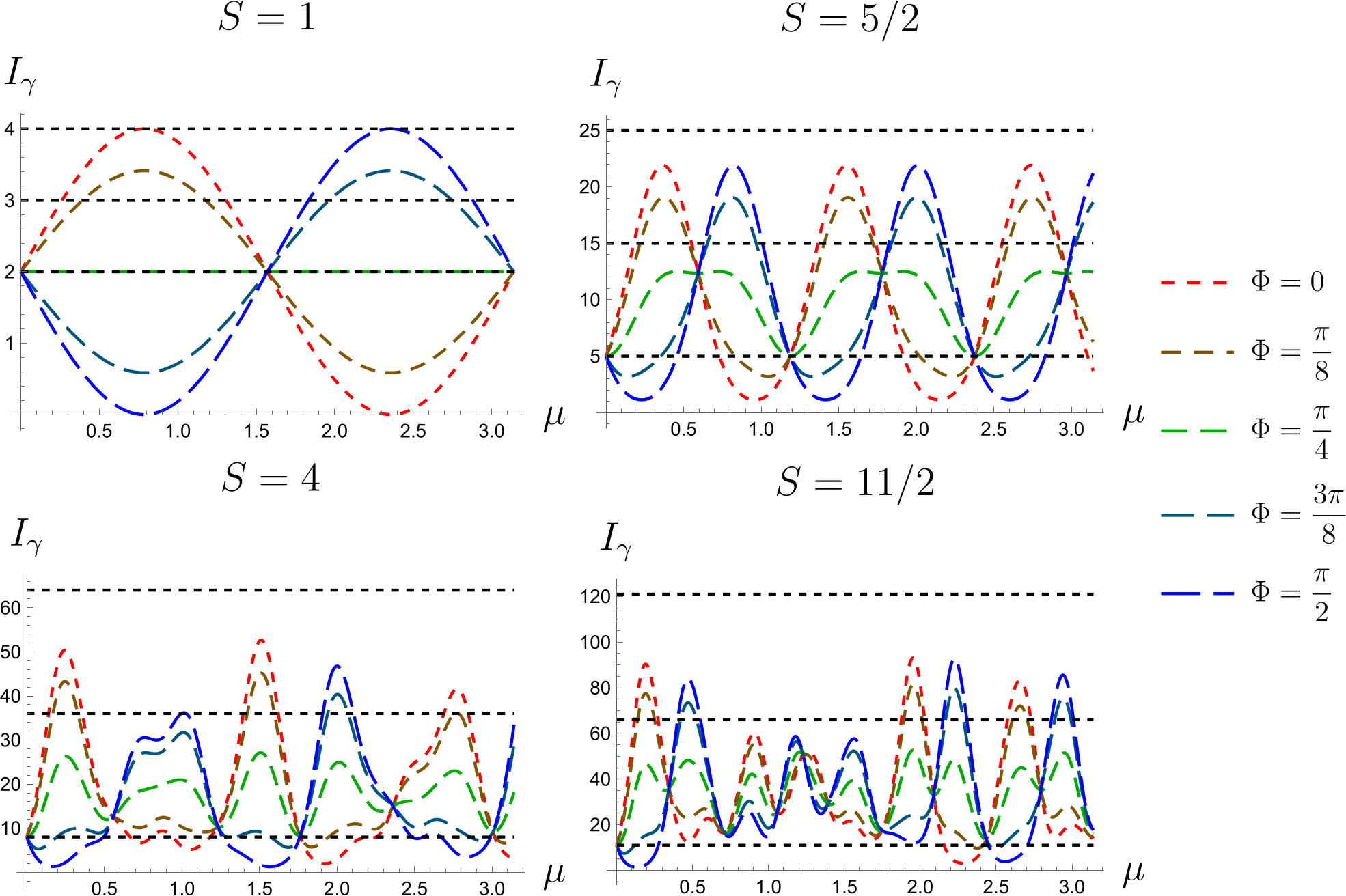
where we use the shorthand notation . The above form allows us to derive the expression for the QFI for the rotation angle around any fixed equatorial axis parametrized by the angle ,
| (29) |
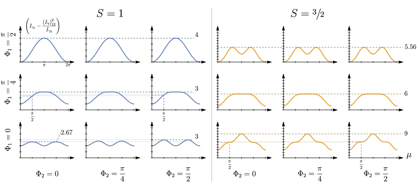
See details in Appendix C. In Fig. 4 we present some properties of the above function for a fixed value of for different values of and . If the squeezing , QFI reaches the value for all probe spins for either or axis, depending on half- or integer-spin of the probe. At the same time the estimation for the orthogonal axis yields QFI at the level of . As grows, the plateau for at around grows and flattens.
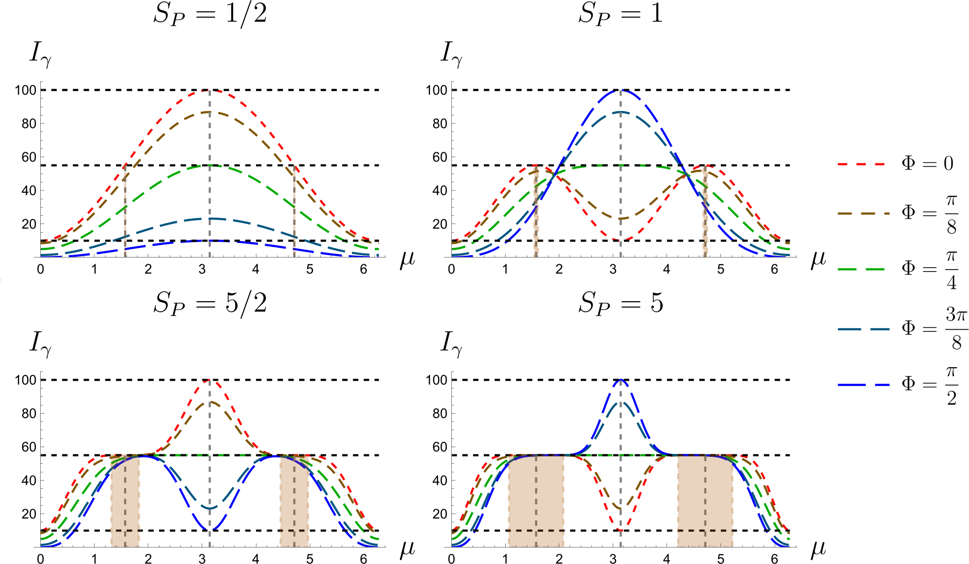
The qualitative features that can be seen from the Fig. 4 will be now formalised, with special attention for maximal squeezing and the half-maximal-squeezing with .
The former case is exceedingly simple and reduces to a formula reminiscent of a sum of coordinates of an ellipse,
| (30) | ||||
| (31) |
bounded from above and below by
| (32) |
where the axes for which the bounds are saturated depend solely on . More precisely, axis is optimal for half-spins, whereas axis reaches optimality for integer spins. This aligns neatly with the properties found for the same axes for one-spin case.
In the less obvious case of the half-maximal squeezing, we find that around the QFI achieves a plateau at a level between the linear and quadratic scaling with the number of spins . The observation is made rigorous by considering an approximation of the QFI with and ,
| (33) | ||||
| (34) | ||||
| (35) |
with the approximation achieved by Taylor expansion around in the lowest order, by noting that vanishes in the limit of large , and by noting that justifies neglecting the term of order . This provides the formal demonstration that the QFI is flat around and becomes progressively more flat for large probe spins. The final line demonstrates that we are exactly at the “optimal” value halfway between the Heisenberg and the classical scalings, giving a stable region within which rotation around any axis can be estimated. In particular, in the stable region, one still retains for . Similar QFI values for the estimation of the rotation angle with fixed rotation axis using states at half-maximal squeezing have been recently reported in [55]. Note that the independence of QFI from the choice of the rotation exhibited by the SRU procedure mimics the behaviour of QFI for SU(1,1) interferometric protocol, where any direction of displacement has the same high value of QFI, allowing for estimation with enhanced sensitivity in arbitrary direction. As such the results we demonstrate for arbitrary equatorial axis can be seen as an extension of results from [55].
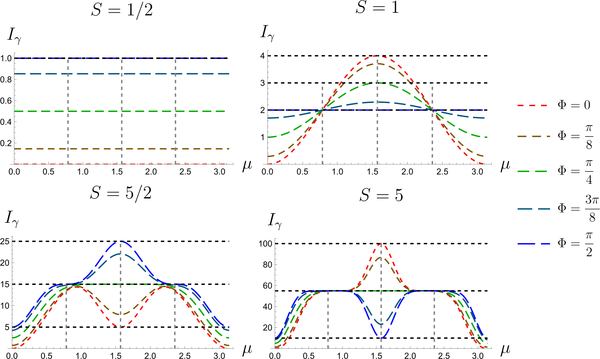
It is instructive to compare the expression (29) with a general formula for the QFI for a single spin,
| (36) |
which is almost identical except for the replacement and some minor changes in the powers and trigonometric functions of the angle . The full derivation of this expression is provided in Appendix D. Most importantly, the analysis concerning the plateau applies without modification for . This suggests that the state presented in the middle panel of Fig. 2, similar in the qualitative properties of its Wigner function to the compass state [56], may be of independent interest.
3.3 Different ways of encoding a relative rotation
In [57] it was pointed out that different ways of coding a relative phase between the two modes in an interferometer can lead to different values of the QFI and hence the sensitivity: if the first arm acquires a phase and the second a phase , the minimal error for estimating was shown to be substantially smaller than if the first arm carries and the second the phase 0. From the classical perspective of a Mach-Zehnder interferometer one would expect that only the relative phase between the two arms matters, because that is all the resulting interference pattern in the two output ports of the interferometer depends on. Quantum-mechanically, however, the two states created are different and can hence lead to different QFI. This implies that there must be measurement schemes that provide higher sensitivity than the usual closing of the interferometer and detection of intensities in the output ports.
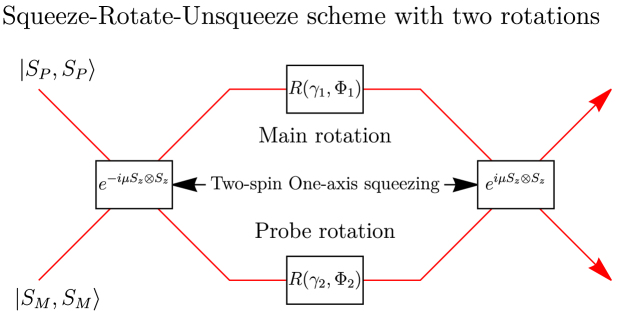
The analogous situation was later studied in the context of SU(1,1) interferometry in [58]. More generally, the second mode or spin can be considered a quantum reference frame [59, 60, 61] that need not be in a classical state and can even be entangled with the main system, i.e. the first mode or spin. Here we investigate a similar question that may arise in the proposed SRU protocol. We consider a rotation on the main spin and an additional rotation on the probe spin. Within this context we consider the multiparameter estimation problem for .
The quantum Fisher information matrix reads
| (37) |
where for convenience we dropped the arguments. The diagonal elements are given by the already known expressions for the main spin
| (38) | ||||
and similarly for , with the roles of and swapped,
| (39) | ||||
The off-diagonal terms can be found as the covariance between and ,
| (40) | ||||
From these the lower bounds on the variance of the estimators of and angles, calculated from positivity of the primary minors of , are given as
| (41) |
We note that and therefore can be set to zero by setting or . Next, we may focus on the denominator of the first of the expressions (41) and its qualitative properties by studying the case of for values and (see Fig. 7). For and we can see clear dependence of the maximal value on the angle , with minimum of and maximum of , coinciding with already known maximum in the single-parameter estimation in similar setting. For we see the already known central maximum with the value . However, a small change can be seen at half-squeezing, . It follows from the fact that the correction term is propotional to , which vanishes for coherent and maximally mixed states, and , respectively. A similar dependence can be seen for . The effect, however, is diminished as the corrections are linear in both main and auxiliary spin, thus not significant in comparison to quadratic terms. Furthermore, they depend on . For we have the maxima of this expression attained at with , smaller than the leading order of , thus negligible for .
In order to draw a proper analogy between a phase difference of the bosonic interferometry, considered in [57], and the rotation angle difference in the introduced SRU scheme, one has to note that such a difference is not well defined, unless we set . In such a case one can consider sensitivity bounds for the relative rotation, . If we assume that the estimators for both rotations are uncorrelated, , we may proceed to find
| (42) |
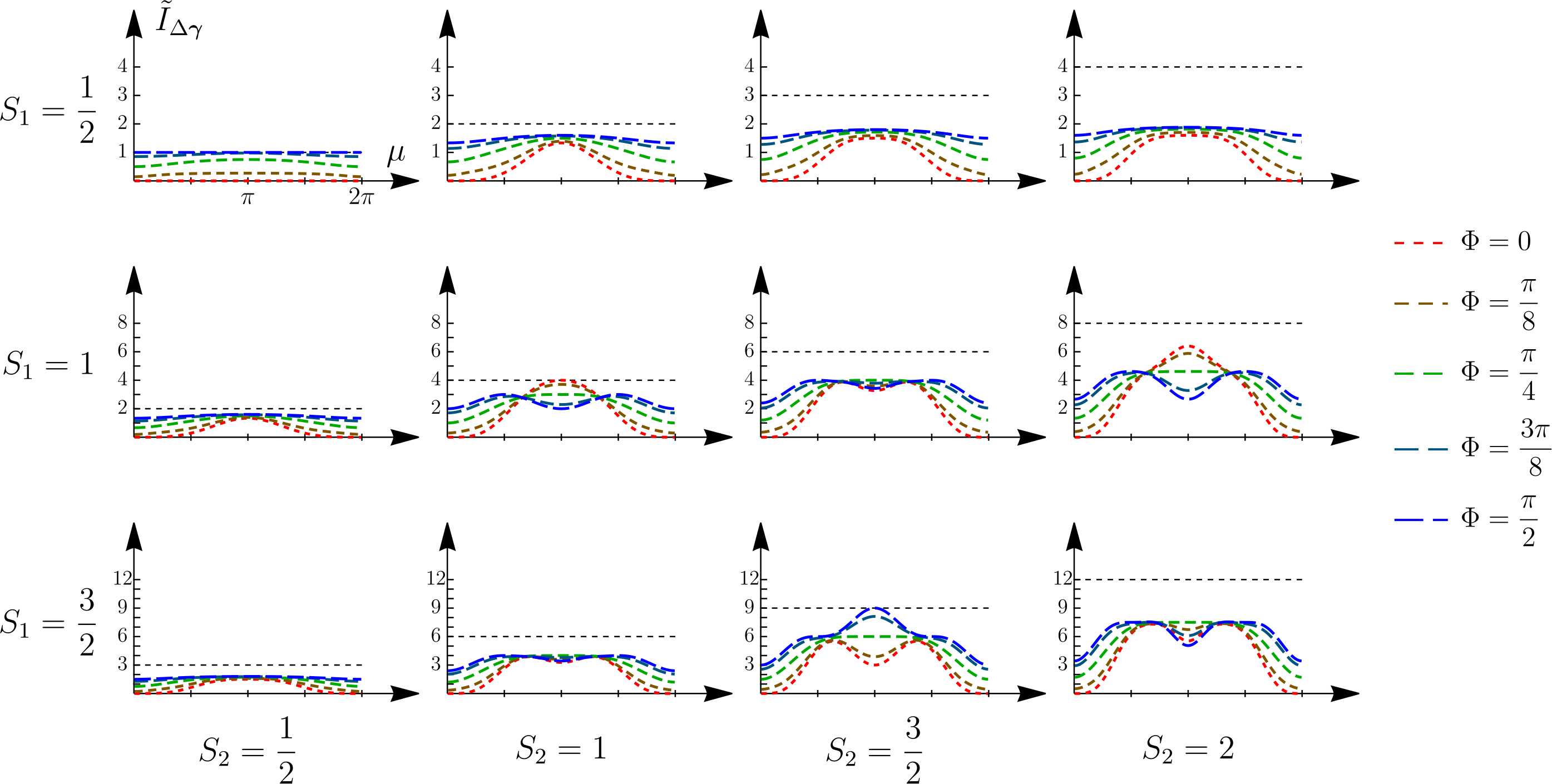
The following expression is depicted in Fig. 8. Note that for equal spins, , the bound behaves similarly to the Fisher information as depicted in 4. In particular, we still see the plateau region around the value for half-squeezing for any axis angle . Similar plateau regions persist for any combination of . Finally, we note that for being half-integer the central maximum is replaced by an indent for both and .
On the other hand, if we allow covariance to be non-zero, by considering the semipositivity condition (16) we find the bounds on covariance given in a compact way by
| (43) |
Based on this it is possible to consider another extreme case, where we allow one of the variances to saturate the bound, eg. , which implies , the bounds for variance of the rotation difference are changed to
| (44) |
which has been plotted with respect to in Fig. 9 for several values of and .
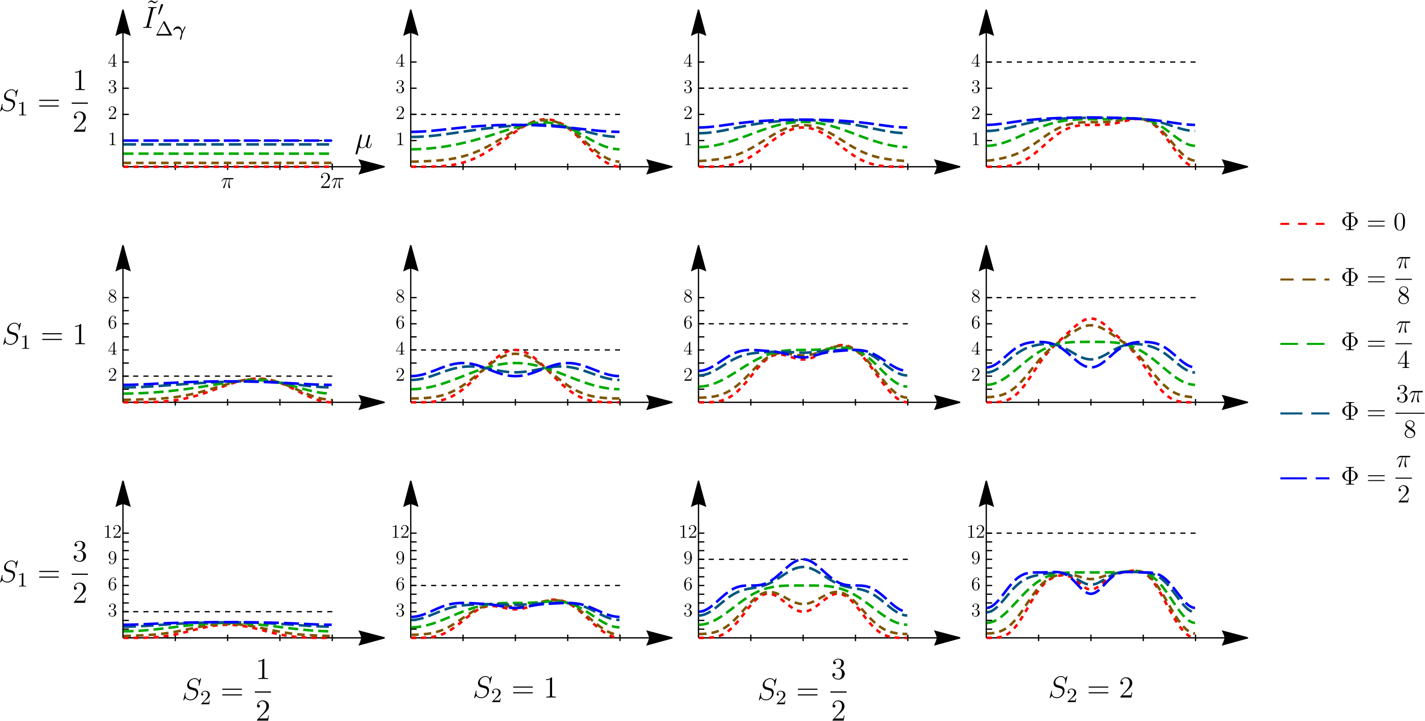
In this case we again see similarity between the plots from Fig. 4 and the equal-spin situations. This time, however, we note that there is an apparent asymmetry resulting in higher values of for values of squeezing closer to rather than . This asymmetry would have been resolved by plotting with up to and can be justified by a heuristic drawn from a single-spin squeezing. Note that squeezing for integer-spins is exactly periodic with period , ie. state returns to itself when . For half-integers the situation is different – squeezing of yields a coherent state, but an antipodal one. Thus, a joint evolution of squeezed integer spin and a half-integer spin is essentially periodic with a period of . In this case we observe the same phenomenon, extended due to the use of two-spin instead of single-spin squeezing.
3.4 Axis angle estimation and sum rule
As we have seen, the SRU protocol allows for a QFI for rotation angle estimation that scales quadratically with the number of systems for any equatorial axis of rotation. It is natural to ask whether it also provides an advantage in the task of rotation axis estimation. In this section we shortly note the properties of the SRU protocol found for this problem in the 2-spin setting. Closed expressions for the general case are hard to obtain, thus we will limit our considerations to a particularly compelling case. First, it is easy to demonstrate that the scaling of the single-parameter QFI for the estimation of the rotation axis angle depends on the angle of rotation ,
| (45) |
suggesting that the case is optimal. This is not the case as , scaling linearly with the size of the spin system. Consider then the intermediate case with the state turned by a quarter-turn, , which yields
| (46) | ||||
This expression can be compared with a similar Eq.(29). Their sum becomes fully independent from the choice of the rotation axis ,
| (47) |
which shows a peculiar sum-rule: For a constant squeezing parameter, the sum of QFI for rotation angle and the axis angle depends only on the squeezing parameter , which can be understood as a trade-off or an uncertainty relation. The better the sensitivity in the estimation of the rotation angle, the harder it gets to determine the axis of rotation.
3.5 Compatibility of measurements in multivariate estimation problem
3.5.1 Compatibility of rotation angle and axis angle estimation
One may further ask for general attainability of the Cramer-Rao bounds in a scenario where one intends to estimate and simultaneously, based on the commutation of SLDs on average as in eq. (18). Due to the inaccessibility of a closed-formed expressions we conducted a numerical investigation based for selected values of the spin (equal for both spins, ). The results are presented in Fig. 10.
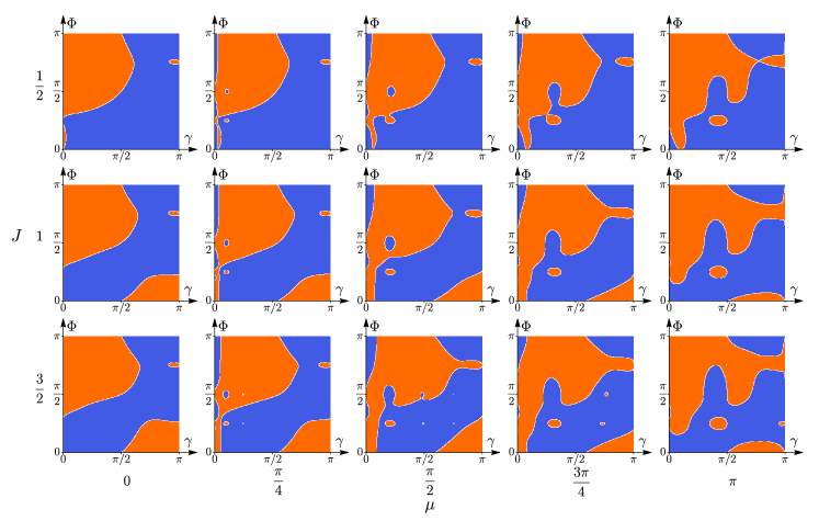
By looking at the plots we see one important feature – there exist regions for which the SLDs commute on average, namely the border lines between the orange and blue regions. This property is not exhibited by the SU(1,1) interferometry. Furthermore, it is useful to note that for for almost any value of there exists a corresponding , for which the SLDs commute. Nevertheless, the structure of regions for which the SLDs commute suggests a need for numerical determination of the saturating measurement in each case.
3.5.2 Compatibility of estimation of two noncommuting rotations
One may also consider the question of estimating rotations with respect to the and axes by angles and , respectively. This bears the closest similarity to the SU(1,1) displacement detection scheme, with two rotations with orthogonal rotation directions in analogy to and quadratures. As we are working with displacements from SU(2) group, we may implicitly define operators and as
| (48) | ||||
where . It is easily shown that
| (49) |
Since each of the operators is proportional to a generator of the group, one can decompose the commutator into the sum of generators,
| (50) |
with
| (51) | ||||
| (52) | ||||
| (53) |
The general expression for the commutator is then given by
| (54) |
Using simple trigonometric limits of the type one finds that
| (55) |
Thanks to this and the alignment of the initial state with the axis we can say that for rotations with rotation angles close to the SLDs commute on average,
| (56) |
which guarantees the existence of a measurement that saturates the multivariate QCRB.
3.6 Axis estimation in the context of estimation with time reversal
Consider Eq.(46) and observe that by setting we get the maximal value of the sum, which can be also re-expressed in terms of the number of half-spin subsystems,
| (57) |
which would suggest exceeding the Heisenberg limit of . This is not the case, as one can rewrite the rotation generated by as
| (58) |
to notice that the rotation of the angle is imprinted twice on the state. One thus deviates from the standard protocol that leads to the HL. The double imprinting comes with a slight twist: the evolution is first forward in time and the second time backward in time. In other words, we have double imprinting of with time reversal. This can be also interpreted as estimation of the parameter of a Hamiltonian evolution acting as a superoperator on a different, fixed Hamiltonian evolution.
We wish to calculate the optimal value of Fisher information from the state and its derivative given by
| (59) |
Assume that is a constant Hamiltonian rescaled in such a way that its eigenvalues satisfy , and the free parameters are the input state and the auxiliary Hamiltonian . Inspection of these expressions shows that whenever . This suggests that the largest value of should be connected to in a suitable metric.
In order to bound the optimal value of from below we introduce an Ansatz of and assume that the auxiliary Hamiltonian does not mix the subspace with its complement. Explicit calculations in Appendix F show that by setting on the two-dimensional subspace mentioned above we find the maximum of the Fisher information,
| (60) |
which is well above the value of demonstrated for the axis estimation problem.
3.7 Numerical study of two-axis squeezing
For completeness, we shortly consider a variant of the SRU protocol where instead of one-axis squeezing we utilize the two-axis squeezing operator. The full protocol is now defined as
| (61) |
in analogy to the SRU protocol defined in (19). Here the squeezing Hamiltonian has been changed to and the input state is a spin coherent state pointing along the axis, following the preparation presented in [16]. Therein, the authors have demonstrated that the variance of a spin in a selected direction orthogonal to the main axis of the squeezed state for large spins approaches a constant. Later the two-axis squeezing has been studied theoretically [62] and only recently an experimental realization has been proposed [63].
In this case analytical treatment is not accessible. Therefore we present a set of plots for selected values of which present the qualitative behaviour of two-axis squeezing. Despite clearly periodic behaviour for and , for larger spins the QFI fails to reach the value of demonstrated to be attainable for one-axis squeezing. Furthermore, despite isolated points at which Fisher information agrees for different rotation axes, no stable plateaus can be found.
4 Concluding Remarks
In this work we have translated interferometry, understood by Caves as a displacement detector [6], to the field of spin-rotation estimation. The introduced squeeze-rotate-unsqueeze protocol for two- and one-spin one-axis squeezing, analogous to the squeeze-displace-unsqueeze procedure applied in the interferometry, has been demonstrated to provide an advantage over the best classical scheme. This is evidenced by the Quantum Fisher Information (QFI) approaching a scaling with the square of the size of the system ("the Heisenberg scaling”), as opposed to the linear scaling of the Standard Quantum Limit.
Most importantly, for the specific intermediate value of squeezing, , we have found simultaneous quadratic scaling of the single-parameter values
of the QFI for the estimation of the rotation angles around all equatorial axes, which can be compared to the
simultaneous
amplification of displacements
in an arbitrary direction in the phase space for
bosonic systems.
The effect is robust in the sense of the existence of a plateau around the specific squeezing parameter, which grows with the size of the probe system.
Furthermore, we have shown that the introduced scheme provides the advantage of quadratic scaling for rotation-axis estimation given control over the rotation angle. Finally, to provide a more complete picture we have demonstrated the behaviour of the QFI for the SRU protocol with two-axis squeezing, showing lack of crucial properties like saturation of Heisenberg limit or appearance of plateaus.
The SRU protocol for a single-spin can be seen as a special case of the delta-kick squeezing (DKS) protocol introduced in [20]. One has, however, to stress that in our work the inspiration comes from the SU(1,1) displacement detector’s ability to achieve an advantage for arbitrary direction of displacement. Therefore, we have focused on finding stable advantages over a wide range of different axes of rotation. The 2-spin SRU protocol goes beyond DKS, in the sense that the size of the probe spin can be used to control the specific dependence of the QFI on the squeezing parameter , allowing an extension of the plateau of quadratic scaling for an arbitrary rotation axis in the equatorial plane. This allows the estimation of different components of a magnetic field that lead to non-commuting rotations with Heisenberg-limited sensitivity. Future research could extend our investigations in the spirit of [24] to ask for variational generation of spin states which are flexible for rotation-angle estimation over a wide range of axes. Several other open directions are left to pursue in the context of the 2-spin SRU protocol. For instance, one may consider the QFI of the probe system for estimating the rotation angle of the primary system. Another future direction involves seeing joint measurability of noncommuting rotations in the perspective of recent attempts to incorporate Heisenberg uncertainty relations into optimization of measurement errors [64].
Finally, it is interesting to mention a recent experimental effort to generate a four photon state with and tetrahedral symmetry in the polarization-related representation [65]. Although not scalable towards larger , it is an example for efforts towards effective schemes for sensing rotations, even beyond actual spin systems. In this sense our method may prove useful for equivalents of rotations in polarization of multi-photon states using methods for polarization-squeezing [66, 67, 68, 69].
Acknowledgments
JCz and KŻ would like to thank Jan Kołodyński and Rafał Demkowicz-Dobrzański for fruitful discussion, in particular on the topic of multiparameter estimation. KŻ and JCz acknowledge gratefully financial support by Narodowe Centrum Nauki under the grant numbers DEC-2015/18/A/ST2/00274 and 2019/35/O/ST2/01049 and by Foundation for Polish Science under the Team-Net NTQC project.
Appendix A Quantum Fisher information for SDU protocol for one- and two-mode scenario
Based on the expressions provided in [6] it is rudimentary to show that the state of a single-mode bosonic system undergoing the SDU protocol is given by
| (62) |
where and we consider to be a coherent state with displacement equal to . QFI with respect to and is then given by
| (63) |
where and . We see that the QFIs are inversely proportional and the QCRB is saturable only when either or , ie. one of the displacements is estimated around 0.
The two-mode input state is given by
| (64) |
where is the operator representation of a beamsplitter. In this case considerations of QFI and of average SLD commutation yield
| (65) |
and hence, we find that (a) any direction of the form has the same QFI of the form and (b) one cannot saturate the bound above for two directions at once using a single measurement.
The above statements may be seen as contradicting the prior results presented in [6], where it was shown that it is possible to estimate both quadratures better than SNL check sensitivity. However, it is not simultaneous in the sense of saturating the matrix-valued QCRB, but in the sense of saturating two single-parameter QCRBs independently. Using the following set of identities
Caves shows that the measurement of Bell variables and is actually equivalent to introducing a beamsplitter operator , measuring single quadratures independently on the first mode and on the second, and applying beamsplitter on the post-measurement state. With the preparation (64) it is clear that one implements an effective equivalent of two local measurements on two states undergoing independent SDU protocols.
Appendix B Quantum Fisher information for SRU protocol with selected rotation axes and maximal squeezing
We start with the expression for the state after the single-spin SRU protocol with maximal squeezing ,
| (66) |
with . We limit ourselves to . In order to arrive at closed expressions we split the presentation into the cases of integer and half-integer spin. Beginning with the integer case, we bring up a useful formula
which shows that for integer spins
| (67) |
Making use of this formula one can rewrite the squeezed states,
| (68) | ||||
| (69) | ||||
| (70) |
which is clearly a NOON state. Now we consider the case , for which we have , such that the rotation introduces phases to the components,
| (71) |
In the last step we need an additional intermediate calculation,
| (72) | ||||
| (73) | ||||
| (74) |
from which we finally write
| (75) | ||||
| (76) |
The case of is easily resolved by using two formulas,
| (77) |
which lead directly to the expression,
| (78) |
Expressions for half-integer spin are obtained in a similar way with the formula,
| (79) |
which yields a similar form of the maximal squeezing operator,
| (80) |
Appendix C QFI for rotation angle of 2-spin SRU around any equatorial axis
The starting point is the 2-spin state after the SRU protocol,
| (81) |
which in this case turns out to be a simple expression to handle. For brevity we shall write . Making use of this notation consider the squeezed state,
and its derivative,
| (82) | ||||
In order to simplify matters it is useful to substitute by and consider auxiliary sums of the form,
| (83) | ||||||||
with . With these one can express the relevant inner products as
| (84) | ||||
where for brevity we replaced and . Standard algebraic transformations lead to,
| (85) | ||||
which yields the expression (29).
Appendix D QFI for rotation angle of 1-spin SRU around any equatorial axis
In order to calculate the Fisher information for a rotation with respect to an arbitrary equatorial axis for a single spin we resort to the approach of first differentiating the operator and then evaluating its expectation value – an approach that yields less knowledge about the states used to perform the task. Consider that
| (86) |
which translates to
| (87) | ||||
and we recall from (8) that . In this case it is helpful to write out the operators as . Then one obtains
| (88) | ||||
| (89) | ||||
| (90) | ||||
| (91) |
The second inner product can be calculated in a similar manner,
| (92) |
with the first term evaluating to
Appendix E Derivation of QFI for axis estimation
The starting point of this derivation is the calculation of the derivative of the state with respect to the axis angle ,
| (95) | ||||||
The prefactor suggests that the maximum of QFI may occur at . However, by explicit calculation we find that the derivative reads
| (96) | ||||||
and straightforward calculation yields . Thus, we propose another Ansatz of quarter-turn, , which yields the expression for the derivative,
Appendix F Quantum Fisher information for superchannel estimation
Recall the initial setting of the superchannel estimation problem,
| (98) |
where we assume to be a fixed Hamiltonian with the maximal and minimal eigenvalues given by and and as free quantum state and a unitary with a free Hamiltonian , respectively, to be adjusted for maximal QFI for the estimation of . In order to demonstrate the lower bound on this maximum we consider as an equal superposition of the eigenstates related to the extremal eigenvalues. With this assumption we evaluate the inner products relevant to the QFI,
| (99) | ||||
| (100) | ||||
| (101) |
and a similar array of expression for the other product of interest,
| (102) | ||||
| (103) |
At this point we decompose in terms of eigenvectors of ,
| (104) | ||||
| (105) |
Observe that acts on the subsapce spanned by , so it can yield only smaller contributions by mixing with the remaining eigenspaces. Assuming that acts only within the same subspace as allows us to write
| (106) |
In this way we arrive at the expressions,
| (107) | ||||
| (108) |
which, by setting and yield,
| (109) |
and . Therefore, we find the QFI to be equal to
| (110) |
which is higher than the value of found for the axis estimation problem. In order to see that is indeed the maximum achievable value consider a projection operator onto the space connected to the largest and smallest eigenvalues. Within this subspace the indeed acts as a time-reversal operation on one of the imprinting protocols,
| (111) |
and by this virtue the value is reconnected to the standard Hamiltonian estimation problem with doubled time of action.
References
- [1] R. Demkowicz-Dobrzański, K. Banaszek, and R. Schnabel. “Fundamental quantum interferometry bound for the squeezed-light-enhanced gravitational wave detector GEO 600”. Phys. Rev. A 88, 041802 (2013).
- [2] J. Aasi et al. “Enhanced sensitivity of the LIGO gravitational wave detector by using squeezed states of light”. Nature Photonics (2013).
- [3] I. G. Irastorza and J. Redondo. “New experimental approaches in the search for axion-like particles”. Prog. Part. Nucl. Phys. 102, 89–159 (2018).
- [4] S. C. Burd, R. Srinivas, J. J. Bollinger, A. C. Wilson, D. J. Wineland, D. Leibfried, D. H. Slichter, and D. T. C. Allcock. “Quantum amplification of mechanical oscillator motion”. Science 364, 1163–1165 (2019).
- [5] B. Yurke, S. L. McCall, and J. R. Klauder. “SU(2) and SU(1,1) interferometers”. Phys. Rev. A 33, 4033–4054 (1986).
- [6] C. M. Caves. “Reframing SU(1,1) interferometry”. Adv. Quantum Technol. 3, 1900138 (2020).
- [7] M. Tsang and C. M. Caves. “Evading quantum mechanics: Engineering a classical subsystem within a quantum environment”. Phys. Rev. X 2, 031016 (2012).
- [8] G. Agarwal. “Quantum optics”. Quantum Optics. Cambridge University Press. (2013).
- [9] N. Bergeal, F. Schackert, M. Metcalfe, R. Vijay, V. E. Manucharyan, L. Frunzio, D. E. Prober, R. J. Schoelkopf, S. M. Girvin, and M. H. Devoret. “Phase-preserving amplification near the quantum limit with a Josephson ring modulator”. Nature 465, 64–68 (2010).
- [10] A. Roy and M. Devoret. “Quantum-limited parametric amplification with Josephson circuits in the regime of pump depletion”. Phys. Rev. B 98, 045405 (2018).
- [11] R. Vijay, D. H. Slichter, and I. Siddiqi. “Observation of quantum jumps in a superconducting artificial atom”. Phys. Rev. Lett. 106, 110502 (2011).
- [12] M. Renger, S. Pogorzalek, Q. Chen, Y. Nojiri, K. Inomata, Y. Nakamura, M. Partanen, A. Marx, R. Gross, F. Deppe, and K. G. Fedorov. “Beyond the standard quantum limit for parametric amplification of broadband signals”. npj Quantum Inf. 7, 1–7 (2021).
- [13] C. F. Ockeloen-Korppi, E. Damskägg, J.-M. Pirkkalainen, T. T. Heikkilä, F. Massel, and M. A. Sillanpää. “Noiseless quantum measurement and squeezing of microwave fields utilizing mechanical vibrations”. Phys. Rev. Lett. 118, 103601 (2017).
- [14] P. Sikivie. “Experimental tests of the "invisible" axion”. Phys. Rev. Lett. 51, 1415–1417 (1983).
- [15] H. Zheng, M. Silveri, R. T. Brierley, S. M. Girvin, and K. W. Lehnert. “Accelerating dark-matter axion searches with quantum measurement technology” (2016). arXiv:1607.02529.
- [16] M. Kitagawa and M. Ueda. “Squeezed spin states”. Phys. Rev. A 47, 5138–5143 (1993).
- [17] T. Byrnes. “Fractality and macroscopic entanglement in two-component Bose-Einstein condensates”. Phys. Rev. A 88, 023609 (2013).
- [18] H. Kurkjian, K. Pawłowski, A. Sinatra, and P. Treutlein. “Spin squeezing and Einstein-Podolsky-Rosen entanglement of two bimodal condensates in state-dependent potentials”. Phys. Rev. A 88, 043605 (2013).
- [19] A. Sinatra, J.-C. Dornstetter, and Y. Castin. “Spin squeezing in Bose-Einstein condensates: Limits imposed by decoherence and non-zero temperature”. Front. Phys. 7, 86–97 (2011).
- [20] R. Corgier, N. Gaaloul, A. Smerzi, and L. Pezzè. “Delta-kick squeezing”. Phys. Rev. Lett. 127, 183401 (2021).
- [21] T. Bilitewski, L. De Marco, J.-R. Li, K. Matsuda, W. G. Tobias, G. Valtolina, J. Ye, and A. M. Rey. “Dynamical generation of spin squeezing in ultracold dipolar molecules”. Phys. Rev. Lett. 126, 113401 (2021).
- [22] D. Leibfried, M. D. Barrett, T. Schaetz, J. Britton, J. Chiaverini, W. M. Itano, J. D. Jost, C. Langer, and D. J. Wineland. “Toward Heisenberg-limited spectroscopy with multiparticle entangled states”. Science 304, 1476–1478 (2004).
- [23] C. Chryssomalakos, L. Hanotel, E. Guzmán-González, D. Braun, E. Serrano-Ensástiga, and K. Życzkowski. “Symmetric multiqudit states: Stars, entanglement, and rotosensors”. Phys. Rev. A 104, 012407 (2021).
- [24] R. Kaubruegger, P. Silvi, C. Kokail, R. van Bijnen, A. M. Rey, J. Ye, A. M. Kaufman, and P. Zoller. “Variational spin-squeezing algorithms on programmable quantum sensors”. Phys. Rev. Lett. 123, 260505 (2019).
- [25] M. F. Riedel, P. Böhi, Y. Li, T. W. Hänsch, A. Sinatra, and P. Treutlein. “Atom-chip-based generation of entanglement for quantum metrology”. Nature (2010).
- [26] S. Colombo, E. Pedrozo-Peñafiel, A. F. Adiyatullin na nAff, Z. Li, E. Mendez, C. Shu, and V. Vuletić. “Time-reversal-based quantum metrology with many-body entangled states”. Nature Physics (2022).
- [27] R. Kaubruegger, A. Shankar, D. V. Vasilyev, and P. Zoller. “Optimal and variational multi-parameter quantum metrology and vector field sensing”. arXiv preprint: 2302.07785 (2023).
- [28] J. M. Radcliffe. “Some properties of coherent spin states”. J. Phys. A: Gen. Phys. 4, 313–323 (1971).
- [29] F. T. Arecchi, E. Courtens, R. Gilmore, and H. Thomas. “Atomic coherent states in quantum optics”. Phys. Rev. A 6, 2211–2237 (1972).
- [30] R. Holtz and J. Hanus. “On coherent spin states”. J. Phys. A: Math. Nucl. Gen. 7, L37–L40 (1974).
- [31] W.-M. Zhang, D. H. Feng, and R. Gilmore. “Coherent states: Theory and some applications”. Rev. Mod. Phys. 62, 867–927 (1990).
- [32] G. S. Agarwal. “Relation between atomic coherent-state representation, state multipoles, and generalized phase-space distributions”. Phys. Rev. A 24, 2889–2896 (1981).
- [33] J. P. Dowling, G. S. Agarwal, and W. P. Schleich. “Wigner distribution of a general angular-momentum state: Applications to a collection of two-level atoms”. Phys. Rev. A 49, 4101–4109 (1994).
- [34] J. Davis, M. Kumari, R. B. Mann, and S. Ghose. “Wigner negativity in spin- systems”. Phys. Rev. Research 3, 033134 (2021).
- [35] A. Kenfack and K. Życzkowski. “Negativity of the Wigner function as an indicator of non-classicality”. J. Opt., B Quantum semiclass. 6, 396 (2004).
- [36] J. Kitzinger, M. Chaudhary, M. Kondappan, V. Ivannikov, and T. Byrnes. “Two-axis two-spin squeezed states”. Phys. Rev. Research 2, 033504 (2020).
- [37] C. Helstrom. “Minimum mean-squared error of estimates in quantum statistics”. Phys. Lett. A 25, 101–102 (1967).
- [38] S. L. Braunstein and C. M. Caves. “Statistical distance and the geometry of quantum states”. Phys. Rev. Lett. 72, 3439 (1994).
- [39] S. L. Braunstein, C. M. Caves, and G. J. Milburn. “Generalized uncertainty relations: Theory, examples, and Lorentz invariance”. Annals of Physics 247, 135–173 (1996).
- [40] M. G. A. Paris. “Quantum estimation for quantum technology”. Int. J. Quantum Inf. 7, 125 (2009).
- [41] J. M. E. Fraïsse. “New concepts in quantum-metrology: From coherent averaging to Hamiltonian extensions”. PhD thesis. University of Tubingen. (2017).
- [42] J. Liu, H. Yuan, X.-M. Lu, and X. Wang. “Quantum Fisher information matrix and multiparameter estimation”. J. Phys. A Math. Theor. (2019).
- [43] O. Giraud, P. Braun, and D. Braun. “Quantifying quantumness and the quest for queens of quantum”. New J. Phys. 12, 063005 (2010).
- [44] C. W. Helstrom. “Quantum detection and estimation theory”. J. Stat. Phys. 1, 231–252 (1969).
- [45] A. Holevo. “Probabilistic and statistical aspects of quantum theory”. Edizioni della Normale Pisa. (2011).
- [46] R. Demkowicz-Dobrzański, W. Górecki, and M. Guta. “Multi-parameter estimation beyond Quantum Fisher Information”. J. Phys. A: Math. Theor. 53, 363001 (2020).
- [47] A. S. Holevo. “Statistical decision theory for quantum systems”. J. Multivar. Anal. 3, 337–394 (1973).
- [48] S. Ragy, M. Jarzyna, and R. Demkowicz-Dobrzański. “Compatibility in multiparameter quantum metrology”. Phys. Rev. A 94, 052108 (2016).
- [49] F. Albarelli, J. F. Friel, and A. Datta. “Evaluating the Holevo Cramér-Rao bound for multiparameter quantum metrology”. Phys. Rev. Lett. 123, 200503 (2019).
- [50] M. Tsang, F. Albarelli, and A. Datta. “Quantum Semiparametric Estimation”. Phys. Rev. X 10, 031023 (2020).
- [51] F. Waldner, D. R. Barberis, and H. Yamazaki. “Route to chaos by irregular periods: Simulations of parallel pumping in ferromagnets”. Phys. Rev. A 31, 420–431 (1985).
- [52] M. Kuś, R. Scharf, and F. Haake. “Symmetry versus degree of level repulsion for kicked quantum systems”. Z. Phys. B: Condens. Matter 66, 129–134 (1987).
- [53] F. Haake and D. L. Shepelyansky. “The kicked rotator as a limit of the kicked top”. Europhys. Lett. 5, 671–676 (1988).
- [54] P. A. Braun, P. Gerwinski, F. Haake, and H. Schomerus. “Semiclassics of rotation and torsion”. Z. Phys. B: Condens. Matter 100, 115–127 (1996).
- [55] G. Müller-Rigat, A. K. Srivastava, S. Kurdziałek, G. Rajchel-Mieldzioć, M. Lewenstein, and I. Frérot. “Certifying the quantum fisher information from a given set of mean values: a semidefinite programming approach” (2023). url: arxiv.org/abs/2306.12711v2.
- [56] W. H. Zurek. “Sub-Planck structure in phase space and its relevance for quantum decoherence”. Nature (2001).
- [57] M. Jarzyna and R. Demkowicz-Dobrzański. “Quantum interferometry with and without an external phase reference”. Phys. Rev. A 85, 011801 (2012).
- [58] C. You, S. Adhikari, X. Ma, M. Sasaki, M. Takeoka, and J. P. Dowling. “Conclusive precision bounds for SU(1,1) interferometers”. Phys. Rev. A 99, 042122 (2019).
- [59] Y. Aharonov and T. Kaufherr. “Quantum frames of reference”. Phys. Rev. D 30, 368–385 (1984).
- [60] S. D. Bartlett, T. Rudolph, and R. W. Spekkens. “Reference frames, superselection rules, and quantum information”. Rev. Mod. Phys. 79, 555 (2007).
- [61] F. Giacomini and C. Brukner. “Quantum superposition of spacetimes obeys Einstein’s equivalence principle”. AVS Quantum Science 4, 015601 (2022).
- [62] D. Kajtoch and E. Witkowska. “Quantum dynamics generated by the two-axis countertwisting Hamiltonian”. Phys. Rev. A 92, 013623 (2015).
- [63] T. Hernández Yanes, M. Płodzień, M. Mackoit Sinkevičienė, G. Žlabys, G. Juzeliūnas, and E. Witkowska. “One- and two-axis squeezing via laser coupling in an atomic fermi-hubbard model”. Phys. Rev. Lett. 129, 090403 (2022).
- [64] X.-M. Lu and X. Wang. “Incorporating Heisenberg’s uncertainty principle into quantum multiparameter estimation”. Phys. Rev. Lett. 126, 120503 (2021).
- [65] H. Ferretti, Y. B. Yilmaz, K. Bonsma-Fisher, A. Z. Goldberg, N. Lupu-Gladstein, A. O. T. Pang, L. A. Rozema, and A. M. Steinberg. “Generating a 4-photon tetrahedron state: Towards simultaneous super-sensitivity to non-commuting rotations” (2023). url: arxiv.org/abs/2310.17150v1.
- [66] A. S. Chirkin, A. A. Orlov, and D. Y. Parashchuk. “Quantum theory of two-mode interactions in optically anisotropic media with cubic nonlinearities: Generation of quadrature- and polarization-squeezed light”. Quantum Elec. 23, 870 (1993).
- [67] D. M. Klyshko. “Polarization of light: Fourth-order effects and polarization-squeezed states”. JETP 84, 1065–1079 (1997).
- [68] N. Korolkova, G. Leuchs, R. Loudon, T. C. Ralph, and C. Silberhorn. “Polarization squeezing and continuous-variable polarization entanglement”. Phys. Rev. A 65, 052306 (2002).
- [69] R. Schnabel, W. P. Bowen, N. Treps, T. C. Ralph, H.-A. Bachor, and P. K. Lam. “Stokes-operator-squeezed continuous-variable polarization states”. Phys. Rev. A 67, 012316 (2003).