Deep Learning for Cross-Domain Few-Shot Visual Recognition: A Survey

Abstract.

Deep learning has been highly successful in computer vision with large amounts of labeled data, but struggles with limited labeled training data. To address this, Few-shot learning (FSL) is proposed, but it assumes that all samples (including source and target task data, where target tasks are performed with prior knowledge from source ones) are from the same domain, which is a stringent assumption in the real world. To alleviate this limitation, Cross-domain few-shot learning (CDFSL) has gained attention as it allows source and target data from different domains and label spaces. This paper provides a comprehensive review of CDFSL at the first time, which has received far less attention than FSL due to its unique setup and difficulties. We expect this paper to serve as both a position paper and a tutorial for those doing research in CDFSL. This review first introduces the definition of CDFSL and the issues involved, followed by the core scientific question and challenge. A comprehensive review of validated CDFSL approaches from the existing literature is then presented, along with their detailed descriptions based on a rigorous taxonomy. Furthermore, this paper outlines and discusses several promising directions of CDFSL that deserve further scientific investigation, covering aspects of problem setups, applications and theories.

1. Introduction

During the past decade, under the joint driving force of big image data and the availability of powerful computing hardware, Machine Learning techniques, in particular Deep Learning (LeCun et al., 2015), have brought revolutionary progress for various computer vision tasks including fundamental ones like image classification (Sharma et al., 2018; Wang et al., 2019a), segmentation (Fu and Mui, 1981; Tavera et al., 2022), and synthesis (Magnenat-Thalmann and Thalmann, 2012; Wu et al., 2017), and object detection (Liu et al., 2020a; Gao et al., 2022). For instance, deep learning has achieved (91.10$\%$ top-1 and 99.02$\%$ top-5) accuracy on the ImageNet image classification challenge, exceeding the cognitive abilities of human beings at 95$\%$ top-5. These capabilities are impressive and unprecedented, especially considering the intrinsic advantages of automation, such as processing data at a much larger scale and efficiency than humans. While it appears that the issue has been resolved, it is important to note that this is merely an experimental outcome within a closed dataset. These huge achievements have been credited to supervised deep learning demanding adequate data and labeling, which, however, remains a substantial disparity from the practical implementation. Firstly, data labeling is an expensive and time-consuming process in many fields, including industrial inspection, endangered species identification, and underwater scene analysis. To address this issue, researchers have explored the use of semi-supervised learning algorithms. However, these algorithms often require strict assumptions, such as the smoothness assumption, cluster assumption, manifold assumption, etc., and have high requirements for training data, such as the need for unlabeled data to be from the same category as labeled data and be evenly distributed. These limitations make them challenging to apply in practice. Furthermore, in certain fields, such as medical imaging, military applications, and remote sensing, data privacy concerns can make it difficult to collect large samples, resulting in only a few available samples.

Solving problems with limited supervised information using few-shot learning (FSL) is feasible based on biological evidence (Carey and Bartlett, 1978). Humans have an excellent ability to recognize a new object with only a few samples. For instance, children can easily distinguish between a ”cat” and a ”dog” with only a few pictures, a capability that machines are yet to attain human-like performance. Additionally, in certain scenes such as natural scene images, it is relatively easy to acquire large amounts of data. Researchers are inspired by the rapid learning ability of humans and transfer learning, and hope that deep learning models can quickly learn new categories with only a small number of samples after learning a large amount of data of a certain category. Therefore, the goal of FSL is to leverage prior knowledge to learn new tasks with only a few labeled samples, which has attracted significant attention due to its crucial industrial and academic applications. Since the introduction of this problem in 2006 (Fei-Fei et al., 2006), numerous research methods have been proposed (Wang et al., 2020; Song et al., 2023; Lu et al., 2020; Shu et al., 2018; Parnami and Lee, 2022).

With the development of FSL, limited training data, domain variations, and task modifications make FSL more challenging, leading to the emergence of variants such as semi-supervised FSL (Zhmoginov et al., 2022), unsupervised FSL (Zhu and Koniusz, 2022; Hu et al., 2022), zero-shot learning (ZSL) (Pourpanah et al., 2022), cross-domain FSL (CDFSL) (Tseng et al., 2020; Guo et al., 2020), and more. These variants are regarded as distinctive cases of FSL tasks in terms of both samples and domain learning. CDFSL addresses the performance degradation in FSL due to domain gaps between auxiliary data that provide prior knowledge and the data in FSL tasks. Figure 1 illustrates the difference between FSL and CDFSL. It has practical applications in many fields with limited supervision information, such as rare cancer detection, video event detection (Yan et al., 2015), object tracking (Bertinetto et al., 2016), and gesture recognition (Pfister et al., 2014). For instance, in the rare cancer detection, obtaining high-quality supervised cancer samples is typically a challenging and expensive process, and there are legal concerns related to patient privacy. In this case, CDFSL can be used to detect rare cancers by utilizing the prior knowledge acquired from a large amount of natural scene images. Therefore, CDFSL has significant practical implications for solving real-world problems. However, it combines the challenges of both transfer learning and FSL, namely the existence of domain gaps and class shift between the auxiliary and target data, and the scarcity of sample sizes in the target domain, making it a more challenging task. Therefore, after researchers evaluated the cross-domain problem in FSL approaches in 2019 (Chen et al., 2019; Nakamura and Harada, 2019), (Tseng et al., 2020) introduced the concept of CDFSL for the first time and proposed corresponding solutions in 2020. Since then, CDFSL has gained widespread attention as a branch of FSL, and numerous related works have been published in top publications. Figure 2 presents the milestones of CDFSL technologies from 2020 to the present, including representative CDFSL methods and related benchmarks.

Figure 1. The difference of few-shot learning and cross-domain few-shot learning.

So far, several existing surveys have made detailed summaries and prospects for FSL (Shu et al., 2018; Wang et al., 2020; Parnami and Lee, 2022; Lu et al., 2020; Song et al., 2023). (Shu et al., 2018) divides FSL into experience learning and concept learning, discussing how to use data from other domains to augment small sample data or rectify existing knowledge. More recently, (Wang et al., 2020) investigates the minimization of empirical risk and define FSL in terms of experience, task, and performance, while also introducing CDFSL as one of the branches of FSL. Both (Parnami and Lee, 2022) and (Lu et al., 2020) introduce CDFSL as a variation of FSL. (Parnami and Lee, 2022) discusses meta-learning, non-meta-learning, and hybrid meta-learning approaches to FSL, and briefly outlines the pioneering work (Tseng et al., 2020) in CDFSL, while (Lu et al., 2020) discusses benchmarks and additional works in CDFSL. Furthermore, a taxonomy is provided from the perspective of prior knowledge in (Song et al., 2023). This paper represents the task shift in FSL as a cross near-domain problem and indicates that existing work cannot address the cross distance-domain problem. All the aforementioned works envision cross-domain issues in FSL as a potential direction. However, there is currently a lack of systematic literature that summarizes and discusses the various related works for CDFSL. Hence, in this period of rapid development, and to stimulate future research and enable newcomers to better understand this challenging problem, this paper presents, for the first time, a comprehensive review of the CDFSL problem. Firstly, this paper collects and analyzs a large body of literature on the topic. The analysis of the reference index reveals that prior to the formal proposal of CDFSL, some works had already focused on the cross-domain issues in the field of FSL (Chen et al., 2019; Nakamura and Harada, 2019). Immediately afterward, its introduction as a branch topic of FSL, CDFSL has gained significant attention and been widely explored. In addition, we define CDFSL using the machine learning definition (Mitchell et al., 1990; Mohri et al., 2018a) and transfer learning theory (Tripuraneni et al., 2020). Secondly, the analysis of a large number of related papers shows that the unique issue of CDFSL is the unreliable two-stage empirical risk minimization problem, which stems from the combination of two factors: (1) a significant discrepancy between the source and target domains(both in terms of the tasks they perform and the domains themselves), (2) the limited amount of supervised information available in the target domain. The details are discussed in Section 2. Hence, all the CDFSL work requires organization through a scientific taxonomy to address its specific challenges. Next, with regard to the question of how to transfer knowledge in CDFSL, this paper provides a comprehensive overview of existing approaches and systematically categorizes them into four distinct categories: instance-guided, parameter-based, feature post-processing and hybrid approaches. To facilitate the understanding of CDFSL and provide a comprehensive evaluation of existing methods, the paper also compiles and introduces a comprehensive collection of relevant datasets and benchmarks. The information related to these datasets and benchmarks is presented in detail, providing valuable insights for researchers and practitioners alike. The paper then goes on to analyze and compare the performance of the different approaches, providing a comprehensive understanding of the state-of-the-art in CDFSL, as discussed in Section 3 and Section 4. Finally, we explore future research directions for CDFSL by considering three perspectives, including problem set-ups, applications, and theories, which provide a comprehensive understanding of the field and its potential for future growth. Contributions of this survey can be summarized as follows:

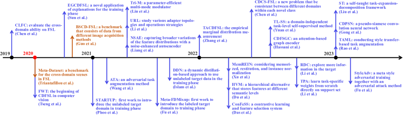
Figure 2. Chronological milestones on CDFSL from 2019 to the present, including representative CDFSL approaches and the related benchmarks. CDFSL was first noticed as a topic in 2020 when two related benchmarks, Meta-Dataset (Triantafillou et al., 2019) and BSCD-FSL (Guo et al., 2020), were released for CDFSL. The pioneering CDFSL work (Tseng et al., 2020) is proposed simultaneously. And (Sun et al., 2021; Guan et al., 2020) are followed proposed, which are the few CDFSL works in 2020. Subsequently, (Phoo and Hariharan, 2020; Islam et al., 2021; Fu et al., 2021; Li et al., 2021a; Liu et al., 2021) explored many new setups for CDFSL like cross multi-domain few-shot learning, etc. And (Liang et al., 2021; Wang and Deng, 2021; Hu et al., 2021; Xu et al., 2021; Du et al., 2021; Das et al., 2022; Chen et al., 2022a) try to improve the CDFSL performance by utilizing different manners. Please see Section 3 for details.

• We analyzed existing CDFSL papers and provided a comprehensive survey, a first of its kind. We also defined CDFSL formally, connecting it to classic ML (Mitchell et al., 1990; Mohri et al., 2018a) and transfer learning theory (Tripuraneni et al., 2020). This helps guide future research in the field.

• We listed relevant learning problems for CDFSL with examples, clarifying their relation and differences. This helps position CDFSL among various learning problems. We also analyzed unique issues and challenges of CDFSL, helping to explore a scientific taxonomy for CDFSL work.

• We conducted an extensive literature review, organizing it into a unified taxonomy based on instance-guided, parameter-based, feature post-processing, and hybrid approaches. We introduced applicable scenarios for each taxonomy, which can help to discuss its pros and cons. We also presented datasets and benchmarks for CDFSL, summarizing insights from performance results, and discussing each category’s pros and cons, improving understanding of CDFSL methods.

• We proposed promising future directions for CDFSL in problem set-ups, applications, and theories, based on current weaknesses and potential improvements.

The remainder of this survey is organized as follows. Section 2 provides an overview of CDFSL, including its formal definition, relevant learning problems, unique issue and challenges, and a taxonomy of existing works in terms of instance, parameter, feature, and hybrid. Section 3 deals with various approaches to CDFSL problems in detail. Section 4 presents performance results followed by the pros and cons of approaches from each category. And Section 5 discusses future directions for CDFSL in terms of set-ups, applications, and theories. Finally, the survey provides conclusions in Section 6.

2. Background

In this section, we first introduce the key concepts related to CDFSL in Section 2.1. And then, we provide formal definitions of the vanilla supervised learning, FSL, and CDFSL problems in Section 2.2 with concrete examples. To differentiate the CDFSL problem from relevant problems, we discuss their relatedness and differences in Section 2.3. In Section 2.4, we discuss the special issue and challenges that make CDFSL difficult. Section 2.5 presents a unified taxonomy according to how existing works handle the unique issue.

2.1. Key Concepts

Before giving our formal definition of CDFSL, we first define two key basic concepts of ‘domain’ and ‘task’  (Pan and Yang, 2009; Yang et al., 2020) as their specific contents may differ between the source and target problem, inspired by the excellent survey from Pan and Yang (Pan and Yang, 2009).

Definition 2.1.1.

Domain. Given a feature space $\mathcal{X}$ and a marginal probability distribution P(X), where $\textit{X}=\{x_{1},x_{2},...,x_{n}\}\subseteq\mathcal{X}$, $n$ is the number of instances. A domain $\mathcal{D}=\{\mathcal{X},\textit{P(X)}\}$ consists of $\mathcal{X}$ and P(X).

Specifically, for an image domain $\mathcal{D}$, the original images I is mapped to a high-dimensional feature space $\mathcal{X}_{I}$. The features $\textit{X}_{I}$ in $\mathcal{X}_{I}$ is a higher-dimensional abstraction of I, and the corresponding marginal probability distribution is $P(X_{I})$. The image domain $\mathcal{D}$ can be expressed as $\mathcal{D}=\{\mathcal{X}_{I},P(X_{I})\}$. In general, difference in $\mathcal{X}_{I}$ or $P(X_{I})$ can lead to the different domain $\mathcal{D}$.

Definition 2.1.2.

Task. Given a domain $\mathcal{D}=\{\mathcal{X},\textit{P(X)}\}$, a task $\mathcal{T}=\{\mathcal{Y},\textit{P(Y|X)}\}$ consists of the label space $\mathcal{Y}$ and the conditional probability distribution P(Y—X), where $\textit{Y}=\{y_{1},y_{2},...,y_{m}\}\in\mathcal{Y}$, $m$ is the number of labels.

Specifically, we use $x$ and $y$ to represent the input data and supervision terget. For example, for a classification task $\mathcal{T}$, all labels $\textit{Y}^{\mathcal{T}}=\{y^{\mathcal{T}}_{1},y^{\mathcal{T}}_{2},...,y^{\mathcal{T}}_{m}\}\in\mathcal{Y}$ are in the label space $\mathcal{Y}$, and P(Y—X) can be learned from the training data D={$x_{i},y_{i}$}, where $x_{i}\in\textit{X}$ and $y_{i}\in\textit{Y}$. From a physical viewpoint, P(Y—X) can be illustrated as a predict function $f(\cdot)$ that is used to predict the corresponding label y for x.

2.2. Problem Definition

In this subsection, we first define the vanilla supervised learning. The definition of FSL is then illustrated before diving into the definition of CDFSL as we consider CDFSL a sub-area of FSL.

Definition 2.2.1.

Vanilla Supervised Learning. Given a domain $\mathcal{D}$, consider a supervised learning task $\mathcal{T}$, a training set $\textit{D}^{train}$, and a test set $\textit{D}^{test}$ , the goal of vanilla supervised learning is to learn a prediction function $f(\cdot)$ for $\mathcal{T}$ on $\textit{D}^{train}$, making $f(\cdot)$ has a good prediction effect on $\textit{D}^{test}$, where $\{\textit{D}^{train},\textit{D}^{test}\}\subseteq\mathcal{D}$.

For example, an image classification task is categorizing new images into a given class using a model learned from training samples. In classic image classification, training set $\textit{D}^{train}$ has enough images per class, like ImageNet with 1000 classes and over 1000 samples per class. Note that the data set D must not be confused with the domain $\mathcal{D}$. An illustration of a vanilla supervised classification problem is shown in Figure 3 (a).

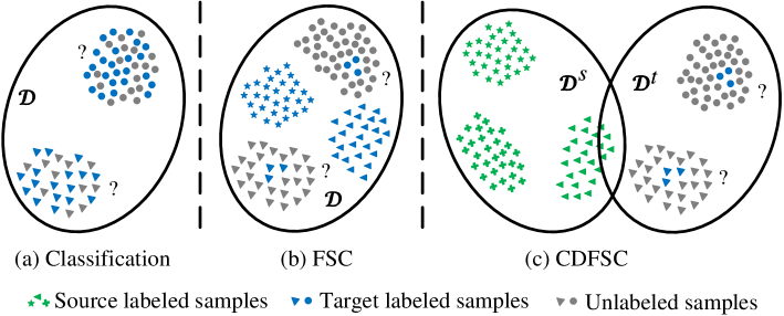
Figure 3. (a) the standard classification, (b) few-shot classification, (c) cross-domain few-shot classification. The different shapes mean the different categories. $\mathcal{D}$ means domain, $\mathcal{D}^{s}$ and $\mathcal{D}^{t}$ specifically represent the source and target domains, respectively. ‘?’ indicates predict the test data.

Like the goal of vanilla supervised learning, the goal of FSL is also to learn a model from the training set $\textit{D}^{train}$ for testing new samples. However, the key difference is that $\textit{D}^{train}$ of FSL only includes very little supervised information, making it a very challenging task. Due to the few samples in $\textit{D}^{train}$, many commonly used supervised algorithms fail to learn satisfying classification models, mainly caused by overfitting. Therefore, it is necessary and natural to introduce some prior knowledge into the FSL task to mitigate the overfitting issue. We call the task of acquiring prior knowledge the auxiliary task $\mathcal{T}^{s}$ (or source task). Usually, the categories of $\mathcal{T}^{s}$ and $\mathcal{T}^{t}$ have no intersection, i.e. $\mathcal{Y}^{s}\cap\mathcal{Y}^{t}=\emptyset$, where $\mathcal{Y}^{s}$ and $\mathcal{Y}^{t}$ are the label sets of $\mathcal{T}^{s}$ and $\mathcal{T}^{t}$, respectively. A formal definition of FSL is given below.

Definition 2.2.2.

Few Shot Learning (FSL). Given a domain $\mathcal{D}$, a task $\mathcal{T}^{t}$ described by a T-specific data set $\textit{D}^{t}$ with only a few supervised information available, and a task $\mathcal{T}^{s}$ described by T-irrelevant auxiliary data set $\textit{D}^{s}$ with sufficient supervised information, FSL aims to learn a function $f(\cdot)$ for $\mathcal{T}^{t}$ by utilizing the few supervised information in $\textit{D}^{t}$ and the prior knowledge in $(\mathcal{T}^{s},\textit{D}^{s})$, where $\{\textit{D}^{t},\textit{D}^{s}\}\subseteq\mathcal{D}$, and $\mathcal{T}^{s}\neq\mathcal{T}^{t}$.

Specifically, take a few-shot classification task $\mathcal{T}^{t}$ as an example, we use the corresponding few-shot data pairs $\{(\textit{x}_{i},\textit{y}_{i})\}^{N^{t}}_{i=1}$ to represent the input data and supervision target. In addition, $\mathcal{T}^{s}$ and $\{(\textit{x}_{i},\textit{y}_{i})\}^{N^{s}}_{i=1}$ are utilized to indicate the conventional classification task and auxiliary data pairs, where $N^{s}\gg N^{t}$. $\mathcal{T}^{t}$ follows a “C-way K-shot” training principle (C indicates the number of classes, K represents the sample numbers in each class). We learn a function $f$($\cdot$) for $\mathcal{T}^{t}$ from $\textit{D}^{t}$ and $(\mathcal{T}^{s},\textit{D}^{s})$. Figure 3 (b) shows the few-shot classification (FSC) problem.

As a branch of FSL, CDFSL also predicts the new samples with the model that is learned by $\{(\textit{x}_{i},\textit{y}_{i})\}^{N^{t}}_{i=1}$ and the prior knowledge from $\{(\textit{x}_{i},\textit{y}_{i})\}^{N^{s}}_{i=1}$. The difference is that $\{(\textit{x}_{i},\textit{y}_{i})\}^{N^{s}}_{i=1}$ and $\{(\textit{x}_{i},\textit{y}_{i})\}^{N^{t}}_{i=1}$ in CDFSL come from two different domains $\mathcal{D}^{s}$ and $\mathcal{D}^{t}$, i.e., $\mathcal{D}^{s}\neq\mathcal{D}^{t}$. Compared to the FSL problem that the data are independent identically distribution (i.i.d.), CDFSL breaks this constraint. Therefore, CDFSL not only inherits the challenges of FSL but also contains its unique cross-domain challenges, making it a more challenging problem. Consequently, numerous conventional FSL algorithms are no longer applicable to CDFSL, which necessitates the development of a viable approach to transfer prior knowledge from the source domain $\mathcal{D}^{s}$ to the target domain $\mathcal{D}^{t}$ without overfitting the model on $\mathcal{D}^{s}$. A definition of CDFSL is formally given below.

Definition 2.2.3.

Cross-Domain Few-Shot learning (CDFSL). Considering a source domain $\mathcal{D}^{s}$ with sufficient supervised information and learning task $\mathcal{T}^{s}$, a target domain $\mathcal{D}^{t}$ with limited supervised information and FSL task $\mathcal{T}^{t}$, the goal of CDFSL is to learn a target perdictive function $f_{T}(\cdot)$ on $\mathcal{D}^{t}$ with the help of the prior knowledge in $(\mathcal{T}^{s},\mathcal{D}^{s})$, where $\mathcal{D}^{s}\neq\mathcal{D}^{t}$, and $\mathcal{T}^{s}\neq\mathcal{T}^{t}$.

In a cross-domain few-shot classification (CDFSC) problem, as shown in Figure 3 (c), we similarly denote a source and a target classification task by $\mathcal{T}^{s}$ and $\mathcal{T}^{t}$, respectively. They are described by the data pairs $\{(\bm{x}_{i}^{s},y^{s}_{i})\}_{i=1}^{N^{s}}\subseteq\mathcal{D}^{s}$ and $\{(\bm{x}_{i}^{t},y^{t}_{i})\}_{i=1}^{N^{t}}\subseteq\mathcal{D}^{t}$, where $N^{s}\gg N^{t}$, $y^{s}_{i}\in\mathcal{Y}^{s}$, $y^{t}_{i}\in\mathcal{Y}^{t}$, $\mathcal{Y}^{t}\bigcap\mathcal{Y}^{s}=\varnothing$ (i.e., the source and target domains do not share the label space). Note that $\mathcal{D}^{t}$ and $\mathcal{D}^{s}$ are sampled from two different probability distributions $p$ and $q$, respectively, where $p\neq q$. The objective of the CDFSC is learning a classifier $f_{T}$($\cdot$) for $\mathcal{T}^{t}$ using $\mathcal{D}^{t}$ and $(\mathcal{T}^{s},\mathcal{D}^{s})$. It addresses the issue that there are no sufficient auxiliary samples in the target domain $\mathcal{D}^{t}$ to provide the proper prior knowledge for $\mathcal{T}^{t}$.

Furthermore, CDFSL can be classified into three broad categories based on why the image distribution differs: Fine-grain based CDFSL (FG), Art-based CDFSL (Art), and Imaging way-based CDFSL (IW). FG-CDFSL pertains to differences in the fine-grained categories between $\mathcal{D}^{s}$ and $\mathcal{D}^{t}$. Specifically, the categories of $\mathcal{D}^{t}$ are the fine-grained classes of a specific variety in $\mathcal{D}^{s}$. A-CDFSL involves differences in artistic expression, such as sketches, natural images, stick figures, oil paintings, and watercolors. And in IW-CDFSL, dissimilarities in imaging modes between $\mathcal{D}^{s}$ and $\mathcal{D}^{t}$ arise when the datasets comprise images of distinct modalities, for instance, natural images in $\mathcal{D}^{s}$ and medical $X$-ray images in $\mathcal{D}^{t}$. IW-CDFSL is generally considered the most challenging of the three categories.

2.3. Closely Related Problems

In this section, we discuss the closely relevant problems. The difference and relatedness between these problems and CDFSL are illustrated in Figure 4.

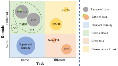
Figure 4. CDFSL related problems. The circles representing target data and its size indicating amount.

Semi-supervised Domain Adaptation (Semi-DA). Semi-DA utilizes a large amount of supervised data in $\mathcal{D}^{s}$, a few labeled data and a large amount of unlabeled data in $\mathcal{D}^{t}$ to improve the performance of $\mathcal{T}$. There are the same label space and different but related sample distributions between $\mathcal{D}^{s}$ and $\mathcal{D}^{t}$, i.e., $\mathcal{D}^{s}\neq\mathcal{D}^{t}$. Similar to Semi-DA, the CDFSL problem also uses a large amount of supervised data in $\mathcal{D}^{s}$ and limited supervised data in $\mathcal{D}^{t}$ to improve the performance of the task $\mathcal{T}$, $\mathcal{D}^{s}\neq\mathcal{D}^{t}$. The difference is that CDFSL does not use many unsupervised samples in the target domain to help with training. Besides, the label space of $\mathcal{D}^{s}$ and $\mathcal{D}^{t}$ are different in the CDFSL problem.

Unsupervised Domain Adaptation (UDA). UDA utilizes a large amount of supervised data in $\mathcal{D}^{s}$ and a large amount of unlabeled data in $\mathcal{D}^{t}$ to improve the performance of $\mathcal{T}$. The distributions between $\mathcal{D}^{s}$ and $\mathcal{D}^{t}$ are different but related, i.e., $\mathcal{D}^{s}\neq\mathcal{D}^{t}$. And they share the same learning tasks. Similar to UDA, CDFSL also uses a large amount of supervised data in $\mathcal{D}^{s}$ to improve the performance of $\mathcal{T}$ in $\mathcal{D}^{t}$, $\mathcal{D}^{s}\neq\mathcal{D}^{t}$. However, $\mathcal{D}^{t}$ in CDFSL has only a few amounts of supervised data, and the tasks of $\mathcal{D}^{s}$ and $\mathcal{D}^{t}$ are different.

Domain Generalization (DG). DG uses a large amount of supervised data in M source domains $\mathcal{D}^{s}=\{\mathcal{D}^{s}_{i}|i=1,...,M\}$ to improve the performance of $\mathcal{T}$ on the unseen $\mathcal{D}^{t}$. The distributions of $\mathcal{D}^{s}$ and $\mathcal{D}^{t}$ are different but related, i.e. $\mathcal{D}^{s}\neq\mathcal{D}^{t}$, and the tasks between $\mathcal{D}^{s}$ and $\mathcal{D}^{t}$ are same. Similar to DG, CDFSL also uses a large amount of supervised data in $\mathcal{D}^{s}$ to improve the performance of $\mathcal{T}$. However, CDFSL is designed to perform well on the special $\mathcal{D}^{t}$ but not all unseen $\mathcal{D}^{t}$, and the source data usually come from one source domain. Furthermore, the tasks of $\mathcal{D}^{s}$ and $\mathcal{D}^{t}$ are different, i.e., $\mathcal{T}^{s}\neq\mathcal{T}^{t}$.

Domain Adaptation Few-shot Learning (DAFSL). DAFSL leverages a significant amount of supervised data in the source domain $\mathcal{D}^{s}$ and a limited number of labeled data in the target domain $\mathcal{D}^{t}$ to enhance the performance of the task $\mathcal{T}$ on $\mathcal{D}^{t}$. Although the distributions of $\mathcal{D}^{s}$ and $\mathcal{D}^{t}$ are different, i.e., $\mathcal{D}^{s}\neq\mathcal{D}^{t}$, the learning tasks remain the same. Similarly, CDFSL utilizes the same data configurations in both domains to train the function for task $\mathcal{T}$. However, in contrast to DAFSL, the learning tasks in $\mathcal{D}^{s}$ and $\mathcal{D}^{t}$ differ in CDFSL.

Multi-task Learning (MTL). MTL utilizes $M$ tasks from $\mathcal{D}$ to improve the performance of every $\mathcal{T}_{i}$ (0 ¡ i $\leq$ $M$). All $\{\mathcal{T}_{i}\}^{M}_{i=1}$ are different but related. Different from MTL, the data of $\mathcal{T}^{s}$ and $\mathcal{T}^{t}$ in CDFSL is from different domains $\mathcal{D}^{s}$ and $\mathcal{D}^{t}$, i.e. $\mathcal{D}^{s}\neq\mathcal{D}^{t}$ and $\mathcal{T}^{s}\neq\mathcal{T}^{t}$, and the supervised data in $\mathcal{D}^{t}$ is limited.

2.4. Unique Issue and Challenge

In machine learning, prediction errors are a common occurrence, making it impossible to achieve perfect predictions, i.e., the empirical risk minimization (ERM) unreliable problem. In this section, we begin by explaining the concept of empirical risk minimization (ERM). Next, we delve into the two-stage empirical risk minimization (TSERM) problem for CDFSL. Finally, we examine the distinct issues and challenges posed by CDFSL.

2.4.1. Empirical Risk Minimization (ERM)

Given an input space $\mathcal{X}$ and label space $\mathcal{Y}$, in which $X$ and $Y$ satisfy the joint probability distribution $P(X,Y)$, a loss function $l(\hat{y},y)$, a hypothesis $h\in\mathcal{H}$ , the risk (expected risk) of hypothesis $h(x)$ is defined as the expected value of the loss function:

(1) $$R(h)=\mathbb{E}[l(h(x),y)]=\int l(h(x),y)dP(x,y),$$

The ultimate goal of the learning algorithm is to find the hypothesis $h^{\ast}$ that minimizes the risk $R(h)$ in the hypothesis space $\mathcal{H}$:

(2) $$h^{\ast}=\text{argmin}_{h\in\mathcal{H}}R(h),$$

Since $P(x,y)$ is unknown, we compute an approximation called empirical risk by averaging the loss function over the training set:

(3) $$\hat{R}(h)=\frac{1}{n}\sum_{i=1}^{n}l(h(x_{i},y_{i})),$$

Therefore, the expected risk is usually infinitely approximated by empirical risk minimization  (Mohri et al., 2018b; Vapnik, 1991), that is, a hypothesis $\hat{h}$ is chosen to minimize the empirical risk:

(4) $$\hat{h}=\text{argmin}_{h\in\mathcal{H}}\hat{R}(h)$$

In FSL, due to limited supervised information, the empirical risk $\hat{R}(h)$ may be far from an approximation of the expected risk $h^{\ast}$, resulting in the overfitting of empirical risk minimization hypothesis $\hat{h}$, i.e., the core problem of FSL is the unreliable empirical risk caused by insufficient supervised data. In current FSL approaches, transfer learning is commonly utilized to address overfitting by incorporating additional datasets to aid in task learning. However, as the tasks differ between the source and target domains, FSL is confronted with knowledge transfer challenges resulting from task shift. This is illustrated in the subsequent two-stage empirical risk minimization problem.

2.4.2. Two-Stage Empirical Risk Minimization (TSERM)

We assume that all tasks share a generic nonlinear feature representation. The two-stage empirical risk minimization (TSERM) aims to transfer knowledge from the source task to the target task by learning this generic feature representation. In the first stage, the primary focus is on learning the general feature representation. The second stage then utilizes the acquired feature representation to construct an optimal hypothesis for the target task.

Specifically, we use $\mathcal{T}^{s}$ and $\mathcal{T}^{t}$ to represent a source task and a target task. TSERM learns two hypotheses $f$ and $h$ in a hypothesis space $\mathcal{H}$, where $f$ learns a shared feature representation in the first stage, and $h$ utilizes it to learn a recognizer in the second stage. For convenience, we use

• $(h^{\dagger},f^{\dagger})=\text{argmin}_{(f,h)\in\mathcal{H}}R(h,f)$ indicates the function that minimizes the expected risk.

• $(h^{\ast},f^{\dagger})$ = $\text{argmin}_{(f,h)\in\mathcal{H}}R(h,f)$ means the function that minimizes the expected risk in $\mathcal{H}$.

• $(\hat{h},\hat{f})=\text{argmin}_{(f,h)\in\mathcal{H}}\hat{R}(h,f)$ represents the function that minimizes the empirical risk in $\mathcal{H}$.

Since $(h^{\dagger},f^{\dagger})$ is unknown, it must be approximated by $(h,f)\in\mathcal{H}$. $(h^{\ast},f^{\dagger})$ represents the most optimal approximation in $\mathcal{H}$, while $(\hat{h},\hat{f})$ represents the empirical risk minimization optimal hypothesis in $\mathcal{H}$. Suppose $(h^{\dagger},f^{\dagger})$, $(h^{\ast},f^{\dagger})$, $(\hat{h},\hat{f})$ are all unique. In the first stage, the empirical risk of $\mathcal{T}^{s}$ is given by the following formula:

(5) $$\hat{R}_{s}(h_{s},f)=\frac{1}{N^{s}}\sum^{N^{s}}_{i=1}l(h_{s}\circ f(x_{i}^{s}),y_{i}^{s}),$$

where $l(\cdot,\cdot)$ is the loss function, $N^{s}$ represents the number of training samples in $\mathcal{T}^{s}$, and $x_{i}^{s}$ and $y_{i}^{s}$ represent the samples and corresponding labels in $\mathcal{T}^{s}$, respectively. $h_{s}$ is the hypothesis of $\mathcal{T}^{s}$, The optimal shared feature extraction function $\hat{f}(\cdot)$ is expressed as $\hat{f}=\text{argmin}_{(f,h_{s})\in\mathcal{H}}\hat{R}_{s}(h_{s},f)$.

In the second stage, the empirical risk of $\mathcal{T}^{t}$ is defined as:

(6) $$\hat{R}_{t}(h_{t},f)=\frac{1}{N^{t}}\sum^{N^{t}}_{i=1}l(h_{t}\circ\hat{f}(x_{i}^{t}),y_{i}^{t}),$$

same as above, $h_{t}$ is the hypothesis of $\mathcal{T}^{t}$, $N^{t}$ denotes the number of training samples for $\mathcal{T}^{t}$, and $x_{i}^{t}$ and $y_{i}^{t}$ represent the samples and corresponding labels in $\mathcal{T}^{t}$, respectively. In the second stage, our goal is to estimate a hypothesis $\hat{h_{t}}=\text{argmin}_{(f,h_{t})\in\mathcal{H}}\hat{R}_{t}(h_{t},\hat{f})$ based on the shared feature representations learned in the first stage. We measure the function $(\hat{h_{t}},\hat{f})$ by the excess error on $\mathcal{T}^{t}$, namely:

(7) $$\mathbb{E}[R_{excess}]=\mathbb{E}[R_{t}(\hat{h_{t}},\hat{f})-R_{t}(h_{t}^{\dagger},f^{\dagger})]$$

$$=\mathbb{E}[R_{t}(h^{\ast}_{t},f^{\dagger})-R_{t}(h^{\dagger}_{t},f^{\dagger})]+\mathbb{E}[R_{t}(\hat{h}_{t},\hat{f})-R_{t}(h^{\ast}_{t},f^{\dagger})],$$

Among them, $R_{t}(\cdot,\cdot)$ represents the expected risk on $\mathcal{T}^{t}$. $R_{excess}$ represents the relationship between the expected risk of $(\hat{h_{t}},\hat{f})$ and the optimal prediction rule $(h_{t}^{\dagger},f^{\dagger})$. Besides, we represents the estimation error with $\mathbb{E}[R_{t}(\hat{h}_{t},\hat{f})-R_{t}(h^{\ast}_{t},f^{\dagger})]$, i.e., minimizing the empirical risk $\hat{R}_{t}(h_{t},f)$ in $\mathcal{H}$ instead of the expected risk $R_{t}(h_{t},f)$, as shown by the blue dotted line in Figure 5.

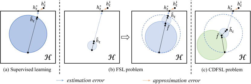
Figure 5. Comparison of vanilla supervised learning, FSL, and CDFSL problem. Solid circles denote distributions in which the data resides (the size means the amount of data), and dotted circles indicate the domain to which the target distribution belongs.

2.4.3. Unique Issue and Challenge

We cannot optimize the approximation error, i.e. $\mathbb{E}[R_{t}(h^{\ast}_{t},f^{\dagger})-R_{t}(h^{\dagger}_{t},f^{\dagger})]$, due to the limitation of $\mathcal{H}$. Therefore, our goal is to optimize the estimation error, i.e. $\mathbb{E}[R_{t}(\hat{h}_{t},\hat{f})-R_{t}(h^{\ast}_{t},f^{\dagger})]$. In Figure 5, the solid black arrow expresses the learning of empirical risk minimization. The solid circles indicate the different data distributions (the size of the circle means the amount of supervised information, the green and blue circles mean the source domain and target domain, respectively). The distribution where the target sample is located is depicted by the blue dotted circle. In Figure 5, (a) shows a vanilla supervised learning problem. It is easy to achieve ERM learning in the case of a large data set. The left part of (b) denotes the FSL problem, where the learning of ERM is not ideal when the amount of data is insufficient. The existing FSL strategy provides a good initialization for the target task through the different but relevant source task, as shown in the right part of Figure 5 (b).

As a result of the domain gaps between the source and target datasets, a novel problem of CDFSL arises, as illustrated in Figure 5(c). As such, it is evident that the CDFSL problem involves both domain gaps and task shifts between the source and target domains, with limited supervised information available in $\mathcal{D}^{t}$. This makes CDFSL have its unique challenges while inheriting the challenges of FSL, namely an unreliable TSERM (estimation error optimization) due to the following factor: the CDFSL problem is characterized by domain gaps and task shifts, leading to a limited correlation between the source and target domains, thereby restricting the shared knowledge between them. As a result, it becomes challenging for the model to identify the optimal function $f$ for task $\mathcal{T}^{t}$ with the support of $\mathcal{D}^{s}$ and $\mathcal{T}^{s}$, where $\mathcal{D}^{s}\neq\mathcal{D}^{t}$ and $\mathcal{T}^{s}\neq\mathcal{T}^{t}$. In other words, the shared knowledge between the source and target domains is challenging to extract.

2.5. Taxonomy

According to the above unique issue and challenge, CDFSL aims at mining as much shared knowledge as possible and finding the optimal $f$ for the target domain. Based on this consideration and to answer the question “how to transfer”, all the CDFSL techniques are categorized into the following four in this paper, as shown in Figure 6:

• Instance-guided Approaches. The model learns the optimal features from more diverse samples by introducing a subset of instances.

• Parameter-based Approaches. Optimizing the model parameters and excluding some regions of $\mathcal{H}$ where the optimal function is unlikely to exist, reduces the scope of $\mathcal{H}$.

• Feature Post-processing Approaches. Learning a feature function from the source domain and performing subsequent processing on its features. A new feature closest to $f^{\dagger}$ is obtained through post-processing operations.

• Hybrid Approaches. Combining the multiple strategies from the above three categories.

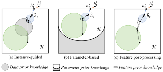
Figure 6. Different perspectives on how the CDFSL approaches find the optimal features.

Accordingly, existing works can be categorized into a unified taxonomy. In the following sections, we will detail each category, performances, future works, and conclusion. The main contents of this paper are shown in Figure 7.

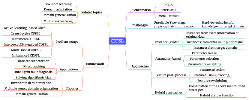
Figure 7. Outline of our survey. The main contents include the benchmarks, challenges, related topics, methodology, and future works of CDFSL.

3. Approaches

CDFSL offers a unified solution to both cross-domain and few-shot learning problems. Based on the analysis of unique issue and challenges, we present a classification criterion for CDFSL algorithms, dividing them into four categories: instance-guided, parameter-based, feature post-processing, and hybrid approaches. The overview of CDFSL is depicted in Figure 8.

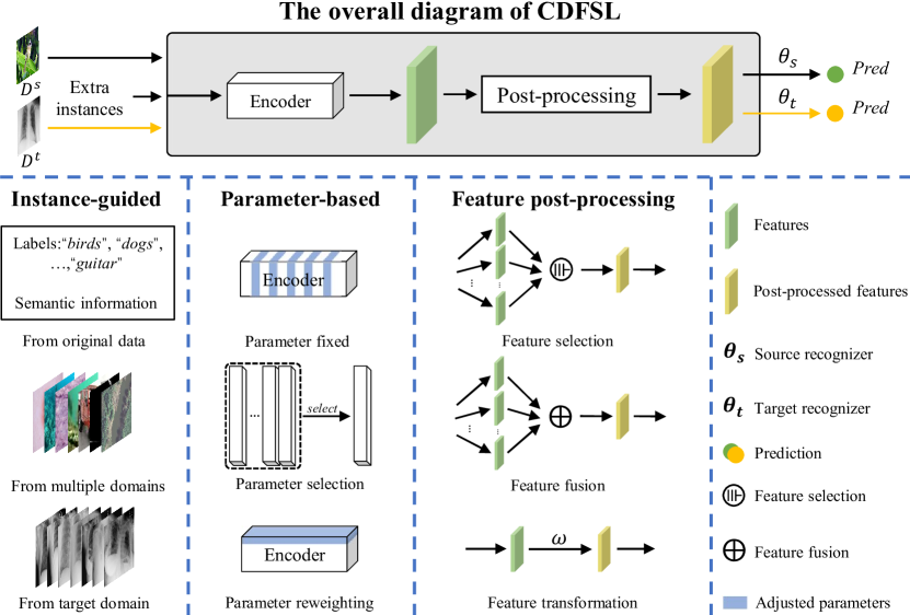
Figure 8. An overall diagram of the CDFSL method. Firstly, the existing techniques pre-train the feature extractor on the source domain. Secondly, they fine-tune the feature extractor and train a novel recognizer on the target domain with limited labels. We classify existing CDFSL methods into Instance-guided, parameter-based, and feature post-processing.

3.1. Instance-guided Approaches

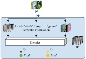
Figure 9. The different categories of instance-guided approaches. Instances are from different sources. $\theta$ means the recognizer.

This section presents approaches that learn the shared feature representation by incorporating additional valid instances from various sources, including the source domain, target domain, and additional domains. The diverse information provided by these sources offers practical guidance for finding shared features. For example, information from the source domain, often obtained from different modalities and views, expands the practical information and facilitates the learning of shared features. Furthermore, by incorporating information from the target domain, the model can better understand the target domain and generalize to it more easily. Information from multiple domains enables the model to learn a shared representation from various domains, making the learned features more generalizable. These approaches are illustrated in Figure 9, and their details are presented in Table 1.

Table 1. Representative instance-guided CDFSL approaches. ‘FG’, ‘Art’ and ‘IW’ indicate that evaluation of Fine-grain based CDFSL (FG), Art-based CDFSL (Art) and imaging way-based CDFSL (IW), respectively. ‘CWUT’ means Channel-Wise Uniform Transformation. And ‘KBS’ represents Knowledge-Based Systems.

Methods	Venue	Instances from	Introduced information	Loss function	FG	Art	IW
TriAE (Guan et al., 2020)	ACCV 2020	Original data	Labels	$L_{2}$		✓
NSAE (Liang et al., 2021)	ICCV 2021	Original data	Generated images	BSR & Log	✓		✓
SET-RCL (Li et al., 2022c)	ACM MM 2022	Original data	CWUT	CE & Contrastive & Log	✓		✓
MDKT (Li et al., 2021b)	Neurocomputing 2021	Original data	Class semantic	CE	✓
CDPSN (Gong et al., 2023)	Scientific Reports 2023	Original data	Sketch map	CE			✓
ST (Liu et al., 2023)	KBS 2023	Original data	Transformation	CE	✓
DAML (Lee et al., 2022)	ICASSP 2022	Multiple domains	3 other datasets	CE	✓	✓
MCDFSL (Xu and Liu, 2022)	arXiv 2022	Multiple domains	7 auxiliary datasets	BSR & Perceptual & Style			✓
STARTUP (Phoo and Hariharan, 2020)	ICLR 2021	Target domain	Unlabeled target data	CE & KL & SimCLR			✓
DDN (Islam et al., 2021)	NIPS 2021	Target domain	Unlabeled target data	CE			✓
DSL (Yao, 2021)	ICLR 2022	Target domain	Multiple targets	RCE & Binary KLD	✓
UD (Hu et al., 2021)	arXiv 2021	Target domain	Unlabeled target data	Log		✓

3.1.1. Instances from Extra Information of Original Data

Some approaches involve the use of additional information from the original data, such as semantic and visual information, to enhance the performance of FSL tasks, as shown in Figure 10. Among them, some works extract this extra information through reconstructed instances, as depicted in the green background area of the Figure 10. For example, in (Guan et al., 2020), a Triplet Autoencoder (TriAE) is utilized to learn a shared feature representation. It incorporates both source and target instances, and leverages semantic information as an intermediate bridge. In (Liang et al., 2021), an autoencoder is used to reconstruct the input data, and the reconstructed data is then utilized as additional visual information to aid in the training process and learn the shared feature representation. And (Li et al., 2022c) distills the knowledge of multiple tasks/domain-specific networks into a single network. This is achieved by aligning the representations of the single network with the task/domain-specific ones using small capacity adapters.

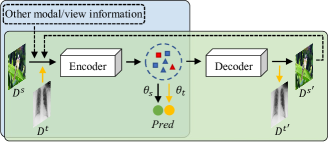
Figure 10. Instances from extra information of original data. The extra information can be from generation model (green area) or other modal like texts (blue part). Dotted lines indicate the process of additional information introduction.

Meanwhile, other works directly add additional information to the model, as shown in the blue part of Figure 10. For instance, (Li et al., 2021b) presents a model that integrates visual and semantic information to recognize target categories, and utilizes weight imprinting for future fine-tuning. Furthermore, in (Gong et al., 2023), the original image and its corresponding sketch map are processed separately by different branches of the network. The features extracted from the original image are combined with the contour features extracted from the sketch map branch during training, thus improving the accuracy and generalization performance of the model. Moreover, (Liu et al., 2023) proposes a task-expansion-decomposition framework for CD-FSL called the self-taught (ST) approach, which alleviates the problem of non-target guidance by constructing task-oriented metric spaces.

3.1.2. Instances from Multiple Domains

By utilizing instances from multiple domains, a model can learn a general shared representation with broad generalization ability. The Domain-Agnostic Meta Learning (DAML) algorithm, proposed in (Lee et al., 2022), adapts the model to novel classes in seen and unseen domains. In contrast, (Xu and Liu, 2022) introduces unlabeled data from multiple domains into the original source domain to transfer diverse styles, making the model more adaptable to various domains and styles. Moreover, most methods combine multiple strategies together with the multiple-domain introduction strategy, as shown in Section 3.4.

3.1.3. Instances from Target Domain

Approaches that leverage target domain instances aim to uncover the shared information between the source and target domains. Some of these approaches employ a teacher-student network to aid CDFSL learning. For example, in (Phoo and Hariharan, 2020), (illustrated in Figure 11), a self-training method is proposed that utilizes unlabeled target data to improve the source domain representation. It is the first work to introduce the unlabeled target data into the training phase.  (Islam et al., 2021) follows this setting and enforces consistency by comparing predictions of weakly-augmented unlabeled target data from a teacher network to strongly-augmented versions of the same images from a student network. Meanwhile, (Yao, 2021) develops a self-supervised learning approach to fully leverage unlabeled target domain data.

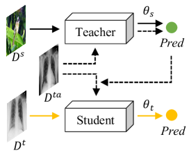
Figure 11. STARTUP (Phoo and Hariharan, 2020) structure. The dotted line represents how to use the auxiliary target data.

Other works integrate all labeled target data directly into the training process. For instance, (Hu et al., 2021) presents a Domain-Switch Learning (DSL) framework that embeds cross-domain scenarios into the training phase in a ”fast switching” manner using multiple target domains.

3.1.4. Discussion and Summary

Instance-guided strategies are chosen based on the availability of data. When the source domain includes extra information such as semantic and visual information, utilizing instances from the original source (as described in Section 3.1.1) is an effective approach. However, in scenarios where extra information is not available, introducing instances from the target domain (as discussed in Section 3.1.3) may be a better option. In cases where target data is scarce or unavailable, utilizing instances from multiple domains (as outlined in Section 3.1.2) can also be helpful.

3.2. Parameter-based Approaches

Parameter-based approaches are designed to reduce the complexity of the hypothesis space by manipulating the model’s parameters to discover shared feature representations. There are three main techniques in this approach, as illustrated in Figure 12: (1) Parameter freeze involves fixing certain model parameters, simplifying the search for shared feature representations, (2) In parameter selection, the most appropriate model is selected from a pool of models based on their parameters, and (3) Parameter Reweighting employs additional parameters to constrain the hypothesis space. Table 2 provides a detailed summary of the methods that fall under this category.

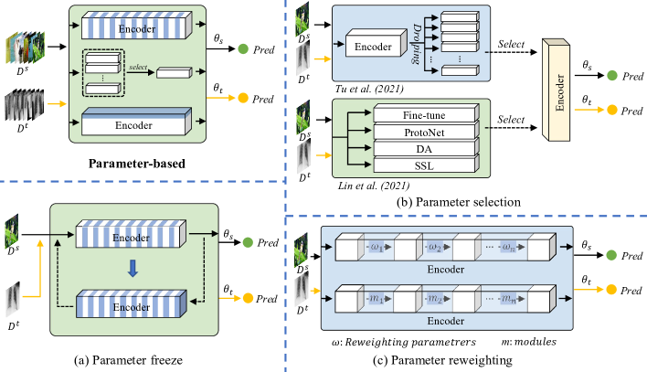
Figure 12. Parameter-based category. (a), (b), and (c) indicate the parameter freeze, parameter selection, and parameter reweighting, respectively.

3.2.1. Parameter Freeze

Parameter freeze is a strategy that restricts the hypothesis space’s complexity by fixing some model parameters. This method is usually used in meta-learning-based approaches, where they alternately freeze some parameters during meta-training and meta-testing phases. Among them, score-based meta transfer-learning (SB-MTL) (Cai et al., 2020) combines transfer-learning and meta-learning by using a MAML-optimized feature encoder and a score-based Graph Neural Network. Some parameters in MAML are frozen in the training phase. And in (Wang et al., 2021), a meta-encoder is alternately frozen and optimized during the inner update phase to learn general features. In addition, other works propose plug-and-play augmentation modules to constrain the hypothesis space. In these works, the core idea of (Tseng et al., 2020) is to asynchronously freeze and update the proposed feature-wise transformation layers and the feature extractor, as shown in Figure 12 (a). Due to the inspiring of (Tseng et al., 2020), many works have improved and enhanced this work. (Yalan and Jijie, 2021) proposes a diversified feature transformation based on the original feature transformation layer to solve the CDFSL problem. And (Chen et al., 2022b) offer two new strategies, FGNN (Flexible GNN) and a new hierarchical residual-like block, for the encoder and metric function of the metric-based network.

3.2.2. Parameter Selection

The parameter selection strategy, as depicted in Figure 12 (b), seeks to identify the most appropriate set of parameters for the target domain to enhance performance. To achieve this, researchers have proposed various methods. For example, in (Tu and Pao, 2021), the authors sample sub-networks by dropping neurons or feature maps, and then choose the most suitable sub-networks to form an ensemble for target domain learning. Additionally, (Lin et al., 2021) proposes a dynamic selection mechanism by sequentially applying multiple state-of-the-art adaptation methods, thereby enabling the configuration of the most appropriate modules for the downstream task.

Table 2. Representative parameter-based CDFSL approaches. ‘NCA’ means Neural Computing and Applications.

Methods	Venue	Strategy	Parameter operation	Loss function	FG	Art	IW
SB-MTL (Cai et al., 2020)	arXiv 2020	Parameter freeze	Freeze partial layers in inner loop and update all network in outer loop	CE			✓
MPL (Wang et al., 2021)	TNNLS 2022	Parameter freeze	Freeze network in inner loop and update it in meta update	CE	✓	✓
FWT (Tseng et al., 2020)	ICLR 2020	Parameter freeze	Alternately update the parameters of the feature-wise transformation layers and backbone	CE	✓
DFTL (Yalan and Jijie, 2021)	ICAICA 2021	Parameter freeze	Following the training setup of (Tseng et al., 2020), and utilize multiple FWT modules in each layers	CE	✓
FGNN (Chen et al., 2022b)	KBS 2022	Parameter freeze	Following the training setup of (Tseng et al., 2020)	Softmax	✓
AugSelect (Tu and Pao, 2021)	Big Data 2021	Parameter selection	Select from multiple sub-network that obtained by dropping feature maps	CE	✓	✓
MAP (Lin et al., 2021)	arXiv 2021	Parameter selection	Select from different modular adaptation pipeline	CE	✓	✓
ReFine (Oh et al., 2022)	CIKM 2022	Parameter reweighting	Re-randomize the top layers of the feature extractor before fine-tuning on the target domain	CE			✓
VDB (Yazdanpanah and Moradi, 2022)	CVPRW 2022	Parameter reweighting	Introducing the ”Visual Domain Bridge” into CNN’s Batch Normalization (BN) layers	CE			✓
AFGR (Sa et al., 2022)	NCA 2022	Parameter reweighting	Reweight the backbone with a residual attention module	CE	✓
TPA (Li et al., 2022b)	CVPR 2022	Parameter reweighting	The task-specific weights are learned to adjust model parameters	CE	✓	✓
ATA (Wang and Deng, 2021)	IJCAI 2021	Parameter reweighting	Insert a plug-and play model-adaptive task augmentation module into backbone	CE	✓		✓
AFA (Hu and Ma, 2022)	ECCV 2022	Parameter reweighting	Use an adversarial feature augmentation module to simulate distribution variations	CE & Gram-matrix	✓		✓
Wave-SAN (Fu et al., 2022b)	arXiv 2022	Parameter reweighting	A StyleAug module is proposed to adjust the parameter	CE & SSL & Style	✓		✓

3.2.3. Parameter Reweighting

As depicted in Figure 12 (c), the parameter reweighting technique optimizes the model’s performance for the target domain by adjusting a limited number of parameters. Various studies have explored this approach to address the cross-domain challenge in few-shot learning. For instance, (Oh et al., 2022) resets the parameters that were learned on the source domain before adapting to the target data. On the other hand, (Yazdanpanah and Moradi, 2022) addresses the internal mismatch issue in BatchNorm by introducing the ”Visual Domain Bridge” concept. Additionally, (Sa et al., 2022) enhances the feature information by stacking a residual attention module into the feature encoder based on the residual network. Another study, (Li et al., 2022b) trains task-specific weights from scratch on a small support set, as opposed to dynamically estimating them. Recent works like (Wang and Deng, 2021) and (Hu and Ma, 2022) propose adversarial methods to address the domain gap in few-shot learning, where (Wang and Deng, 2021) considers the worst-case problem around the source task distribution and (Hu and Ma, 2022) introduces a plug-and-play adversarial feature augmentation (AFA) method. Finally, (Fu et al., 2022b) adjusts the parameters of a novel Style Augmentation (StyleAug) module to achieve better performance in cross-domain few-shot learning.

3.2.4. Discussion and Summary

The parameter freeze strategy, as discussed in Section 3.2.1, is often combined with meta-learning techniques. In the meta-training phase, two pseudo-domains, namely the pseudo-seen and pseudo-unseen domains, are used to simulate the cross-domain scenario. However, it is important to note that both of these domains are derived from the seen domain, resulting in a relatively small domain distance between them. As a result, algorithms that employ this strategy may not be effective in addressing the distant-domain problem in cross-domain few-shot learning (CDFSL).

The parameter selection strategy (Section 3.2.2) aims to adapt to the target domain by selecting the most suitable set of parameters from a pool of options. While this approach can be effective, it has a limited range of parameter sets to choose from, potentially limiting its ability to find the optimal set for the target domain. Moreover, some implementations of this strategy attempt to incorporate various techniques such as semi-supervised learning, domain adaptation, and fine-tuning within a single framework, resulting in a cumbersome and complex approach, making the framework bulky.

The parameter reweighting strategy (Section 3.2.3) seeks to enhance the model’s generalization capability through minimal parameter adjustments. This approach is critical to improving the model’s performance. However, most existing reweighting methods utilize simple structures, which often result in limited improvements in terms of generalization. Therefore, further research is necessary to explore more complex and effective approaches to parameter reweighting in CDFSL.

3.3. Feature Post-processing Approaches

In CDFSL, the transferable feature representation is achieved through post-processing of the original features, as illustrated in Figure 13. The post-processing strategies include feature selection, feature fusion, and feature transformation. Feature selection involves choosing the features from multiple domains that best fit the target domain. Feature fusion combines multiple features to generate a generalized feature representation. Lastly, feature transformation adjusts the original features using learnable weights. Table 3 shows the related works in detail.

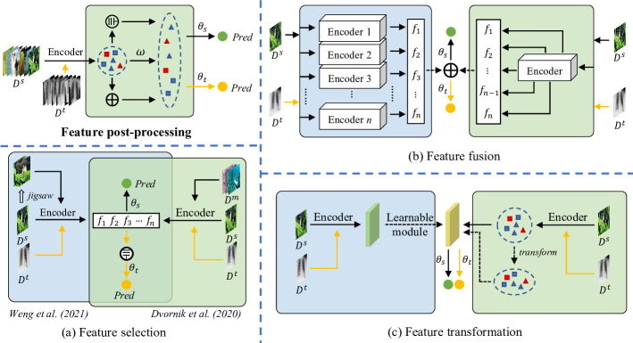
Figure 13. The feature post-processing categories. (a) represents the feature selection, in which the information closest to the shared feature is selected for knowledge transfer. (b) means feature fusion. Various features are stacked to approximate shared features. The left and right parts in (b) show the source of features to be merged. And (c) indicates feature transformation, i.e. the shared feature is obtained through converting the original feature and the left and right parts in (c) means the different convert manners.

3.3.1. Feature Selection

The feature selection strategy involves identifying features closest to the target domain for use as the optimal shared feature representation. This approach is often employed in conjunction with the introduction of multi-domain instances. The strategy first obtains multiple features from different source domains, then selects some of them to aid target domain adaptation. As depicted in Figure 13 (a), (Weng et al., 2021) presents a Representative Multi-Domain Feature Selection (RMFS) algorithm to optimize the multi-domain feature extraction and selection process. While (Dvornik et al., 2020) extracts a multi-domain representation by training a set of feature extractors and then automatically selecting the representations most relevant to the target domain.

3.3.2. Feature Fusion (Stacking)

Feature fusion is an approach used to enhance the generalization ability of models. As depicted in Figure 13 (b), this strategy combines features from different sources or dimensions into a single representation to improve FSL performance on the target domain. Many works, influenced by (Yosinski et al., 2014), believe that features from shallower layers are more transferable than those from deeper layers. Hence, (Adler et al., 2020) proposed the CHEF method which unifies different abstraction levels of a deep neural network into one representation. Additionally, (Zou et al., 2021) combined mid-level features to learn the discriminative information of each sample. Similarly, (Du et al., 2021) used a hierarchical prototype model to combine information from hierarchical memory into final prototype features. Unlike the fusion of shallow layer features, in (Hassani, 2022), the representation of graphs is obtained by augmenting the graphs from sampled tasks into three views: one contextual and two geometric, and encoding each view with a dedicated encoder. Finally, the representations are aggregated into a single graph representation using an attention mechanism. The right part of Figure 13 (b) shows the features from different network layers are fused, whereas the left part shows that features from a set of different networks are stacked.

Table 3. Representative feature post-processing CDFSL approaches. ‘GR’ represents geometrical regularization.

Methods	Venue	Strategy	Feature operation	Loss function	FG	Art	IW
RMFS (Weng et al., 2021)	IC-NIDC 2021	Feature selection	extract the multi-domain features and select from them	CE	✓	✓
SUR (Dvornik et al., 2020)	ECCV 2020	Feature selection	Leverage the multi-domain feature bank to autonomously identify the most pertinent representations	CE	✓	✓
CHEF (Adler et al., 2020)	arXiv 2020	Feature fusion	Accomplish the representation fusion through an ensemble of Hebbian learners operating on diverse layers of the network	CE			✓
MLP (Zou et al., 2021)	ACM MM 2021	Feature fusion	Weight the fusion of mid-level features and investigate a residual-prediction task	CE & $L_{2}$	✓	✓
HVM (Du et al., 2021)	ICLR 2022	Feature fusion	The mid-level features are weighted and fused in a hierarchical prototype model	CE & KL			✓
TACDFSL (Zhang et al., 2022a)	Symmetry 2022	Feature transformation	Propose the adaptive feature distribution transformation	CE			✓
MemREIN (Xu et al., 2021)	IJCAI 2022	Feature transformation	Explore an instance normalization algorithm and a memorized module to transform the original features	CE & Contrastive	✓
RDC (Li et al., 2022a)	CVPR 2022	Feature transformation	Transform and reweight the original features through hyperbolic tangent transformation	CE & KL	✓		✓
StyleAdv (Fu et al., 2023)	arXiv 2023	Feature transformation	Introducing variations to the initial style using the signed style gradients	CE & KL	✓		✓
LRP (Sun et al., 2021)	ICPR 2020	Feature transformation	Develop a model-agnostic explanation-guided training strategy that dynamically finds and emphasizes the features which are important for the predictions	CE	✓
BL-ES (Yuan et al., 2021)	ICME 2021	Feature transformation	An inductive graph network (IGN) is optimizaed by MPGN module, in which include multiple features	BCE & GR	✓		✓
DeepEMD-SA (Ding and Wang, 2021)	ISCIPT 2021	Feature transformation	Employs an attention module to enable interaction between the local features	CE			✓
FUM (Yuan et al., 2022a)	PR 2022	Feature transformation	Using a forget-update module to regulate the features	CE	✓	✓
ConFeSS (Das et al., 2022)	ICLR 2022	Feature transformation	Utilizing a masking module to select relevant information that are more suited to target domain in the features	CE & Divergence			✓
TCT-GCN (Li et al., 2023)	SSRN 2023	Feature transformation	Combining the multi-levelf feature fusion and feature transform	CE	✓		✓
StabPA (Chen et al., 2022a)	ECCV 2022	Feature transformation	Transform features through learning prototypical compact and cross-domain aligned representations	Softmax	✓	✓

3.3.3. Feature Transformation

The feature transformation strategy reweights features to improve performance, as shown in Figure 13 (c). Some methods obtain the weights through a transformation and weighting, e.g. the right part of Figure 13 (c), while others use a learnable module, e.g. the left part of Figure 13 (c). For the former category, in (Zhang et al., 2022a), WDMDS (Wasserstein Distance for Measuring Domain Shift) and MMDMDS (Maximum Mean Discrepancy for Measuring Domain Shift) were proposed to solve CDFSL. (Xu et al., 2021) introduced the MemREIN framework which considers memorization, restitution, and instance normalization, e.g. an instance normalization algorithm is explored to alleviate feature dissimilarity. And (Li et al., 2022a) minimizes task-irrelevant features while keeping more transferrable discriminative information by constructing a non-linear subspace and using a hyperbolic tangent transformation. Furthermore, a novel model-agnostic meta style adversarial training (StyleAdv) method together with a novel style adversarial attack method is proposed for CDFSL in (Fu et al., 2023).

Additionally, there are methods that use a learnable module to determine the feature weights. For example, (Sun et al., 2021) computes explanation scores for intermediate features and reweights them accordingly. (Yuan et al., 2021) acquires the weights by training a bilevel episode strategy (BL-ES) to weight the features. And (Ding and Wang, 2021) employs an attention module upon a local-descriptor-based model called DeepEMD to enable interaction between the local features. Furthermore, (Yuan et al., 2022a) reweights features through extracting relationship embeddings using Forget-Update Modules (FUM). And recently, (Das et al., 2022) employed a masking module to reweight features, selecting those that are more suited to the target domain. And a task context ransformer and graph convolutional network (TCT-GCN) method is proposed in (Li et al., 2023). Lastly, some methods address the CDFSL problem by combining domain adaptation and few-shot learning methods. For instance, (Chen et al., 2022a) proposes stabPA to learn compact, cross-domain aligned representations.

3.3.4. Discussion and Summary

Feature selection strategies can be helpful in selecting the most suitable features for the target domain in the presence of multi-domain or auxiliary views data, as discussed in Section 3.3.1. However, when there are no multiple domains available, features from a single source domain may have limited variability, which means selecting different features from the same source domain may not significantly improve the performance of FSL on the target domain.

The feature fusion strategy (presented in Section 3.3.2) aims to obtain features from multiple sources, either from different layers within a single network or from multiple networks. However, in the case of the former, similarities among the features from the same dataset and network may require effective fusion methods, while in the latter, the use of multiple networks can increase training costs due to the need for simultaneous training.

Feature transformation (introduced in Section 3.3.3) is a common approach when extra network and multi-domain data are not available. It involves reweighting features by assigning new parameters to them, either through simple transformation and weighting, or through a learnable module. However, this strategy only allows limited exploration of shared information as it only reweights the features output from the final layer.

3.4. Hybrid Approaches

Hybrid approaches in CDFSL incorporate the above menthined atrategies, the related technologies is listed in Table 4. Combinations of instance-guided and parameter-based strategies are prevalent in CDFSL. For example, a parameter-efficient multi-mode modulator is proposed in (Liu et al., 2021). First, the modulator is designed to maintain multiple modulation parameters (one for each domain) in a single network, thus achieving single-network multi-domain representation. Second, it divides the modulation parameters into the domain-specific and the domain-cooperative sets to explore the intra-domain information and inter-domain correlations, respectively. Furthermore, (Zhuo et al., 2022) explores a novel target guided dynamic mixup (TGDM) framework to generate the intermediate domain images to help the FSL task learning on the traget domain. In addition, (Peng et al., 2020) learns the meta-learners by utilizing multiple domains, and the meta-learners are combined in the parameter space to be the Initialized parameters of a network used in the target domain. Besides, researchers explore the combination of feature post-process and and parameter-based strategies in CDFSL. (Rao et al., 2023) conducts style transfer-based task augmentation with feature fusion tasks from different tasks and styles and feature modulation module (FM). And in (Wang et al., 2022a), a feature extractor stacking (FES) is proposed to combine information from a backbones collection.

Table 4. Representative hybrid CDFSL approaches. ‘FCS’ represents ‘Frontiers of Computer Science’.

Methods	Venue	Instance-guided	Feature post-process	Parameter-based	Loss function	FG	Art	IW
CosML (Peng et al., 2020)	arXiv 2020	Multiple domains	Feature fusion	✗	CE	✓
URL (Li et al., 2021a)	ICCV 2021	Multiple domains	✗	Parameter reweight	CE & CKA & KL	✓	✓
Meta-FDMixup (Fu et al., 2021)	ACM MM 2021	Labeled target	Feature transformation	✗	CE & KL	✓
Tri-M (Liu et al., 2021)	ICCV 2021	Multiple domains	✗	Parameter reweight	CE	✓	✓
ME-D2N (Fu et al., 2022a)	ACM MM 2022	Labeled target	Feature transformation	✗	CE & KL	✓
TL-SS (Yuan et al., 2022b)	AAAI 2022	Original data	✗	Parameter reweight	CE & Metric	✓		✓
TGDM (Zhuo et al., 2022)	ACM MM 2022	Labeled target	✗	Parameter reweight	CE	✓
TAML (Rao et al., 2023)	arXiv 2023	Multiple domains	Future fusion	Parameter reweight	CE	✓		✓
TKD-Net (Ji et al., 2023)	FCS 2023	Multiple domains	Future fusion	✗	CE & KL & $L_{2}$	✓

3.4.1. Hybrid via Loss Function

Several works solve CDFSL problem not only combine the above mentioned strategies but also with different loss function such as contrastive loss, metric loss, etc. (Fu et al., 2021) advocates utilizing few labeled target data to guide the model learning, and is optimized by CE loss and KL loss. Technically, a novel meta-FDMixup network is proposed to extract the disentangled domain-irrelevant and domain-specific features with a novel disentangle module and a domain classifier. And (Fu et al., 2022a) follows this setup (introduce few labeled target domian data) and proposes a Multi-Expert Domain Decompositional Network (ME-D2N) to solve CDFSL. The loss function also include CE and KL loss. (Zhang et al., 2022b) proposes a Style-aware Episodic Training with Robust Contrastive Learning (SET-RCL) to make the learned model can achieve better adapt to the test tasks with domain-specific styles. And TL-SS strategy (Yuan et al., 2022b) augments multiple views of tasks and proposes a high-order associated encoder (HAE) to generate proper parameters and enables the encoder to flexibly to any unseen tasks. The loss function in this work include CE and a metric loss. Moreover, (Li et al., 2021a) learns a single set of deep universal representations by distilling the knowledge of multiple separately trained networks by using multiple domains after co-aligning their features with the help of adapters and centered kernel alignment. It is optimized by CKA, CE, and KL loss. Furthermore, (Ji et al., 2023) proposes team-knowledge distillation networks (TKD-Net) and explores a strategy to help the cooperation of multiple teachers.

3.4.2. Discussion and Summary

The combination of multiple strategies in CDFSL, as discussed in Section 3.4, can lead to improved performance. For example, the instance-guided strategy is often easily incorporated into various methods, and as such, is frequently combined with other approaches. However, there are also challenges associated with combining strategies. The combination of feature post-processing and parameter-based strategies can be unpredictable and may lead to negative transfer, making it a less frequently explored option. To achieve optimal results, it is essential to avoid negative transfer and carefully consider the combination of strategies in hybrid approaches.

4. Performance

This section provides a comprehensive overview of the evaluation process for models in the field of Cross-Domain Few-Shot Learning (CDFSL). In order to evaluate the effectiveness of these models, we need to examine the appropriate datasets and benchmarks used. This is covered in Section 4.1 and Section 4.2 respectively. In Section 4.3, we delve deeper into a thorough analysis and comparison of the performance of various method categories in the field of CDFSL. This section provides a crucial evaluation of the models, highlighting the strengths and weaknesses of different approaches to address the challenging problem of CDFSL.

4.1. Datasets

The evaluation of CDFSL models is facilitated by the availability of annotated datasets. The comparison of various algorithms and architectures is made fair through the use of these datasets. The continuous growth in complexity, size, annotation number, and transfer difficulty of the datasets represents an ongoing challenge that drives the development of innovative and superior techniques. Table 5 presents a list of the most widely used datasets for the CDFSL problem, and the following sections provide an in-depth description of each:

Table 5. Details of datasets in CDFSL.

Datasets	Derived from	Number of images	Image size	Number of categories	Content	Fields	Reference
miniImageNet	ImageNet	60000	$84\times 84$	100	objects classification	natural scene	(Vinyals et al., 2016)
tieredImageNet	ImageNet	779165	$84\times 84$	608	objects classification	natural scene	(Ren et al., 2018)
Plantae	iNat2017	196613	varying	2101	plants & animals classification	natural scene	(Van Horn et al., 2018)
Places	N/A	10 million	$200\times 200$	400+	scene classification	natural scene	(Zhou et al., 2017)
Stanford Cars	N/A	16185	varying	196	cars fine-grained classification	natural scene	(Krause et al., 2013)
CUB	ImageNet	11788	$84\times 84$	200	birds fine-grained classification	natural scene	(Wah et al., 2011)
CropDiseases	N/A	87000	$256\times 256$	38	crop leaves classification	natural scene	(Mohanty et al., 2016)
EuroSAT	Sentinel-2 satellite	27000	$64\times 64$	10	land classification	remote sensing	(Helber et al., 2019)
ISIC 2018	N/A	11720	$600\times 450$	7	dermoscopic lesion classification	medical	(Tschandl et al., 2018)
ChestX	N/A	100K	$1024\times 1024$	15	lung diseases classification	medical	(Wang et al., 2017)
Omniglot	N/A	25260	$28\times 28$	1623	characters classification	character	(Lake et al., 2011)
FGVC-Aircraft	N/A	10200	varying	100	Aircraft fine-grained classification	natural scene	(Maji et al., 2013)
DTD	N/A	5640	varying	47	textures classification	natural scene	(Cimpoi et al., 2014)
Quick Draw	Quick draw!	50 million	$128\times 128$	345	drawing images classification	Art	(Jongejan et al., 2016)
Fungi	N/A	100000	varying	1394	fungi fine-grained classification	natural scene	(Schroeder and Cui, 2018)
VGG Flower	N/A	8189	varying	102	flowers fine-grained classification	natural scene	(Nilsback and Zisserman, 2008)
Traffic Signs	N/A	50000	varying	43	Traffic signs classification	natural scene	(Houben et al., 2013)
MSCOCO	N/A	1.5 million	varying	80	objects classification	natural scene	(Lin et al., 2014)

• miniImageNet (Vinyals et al., 2016): miniImageNet dataset consists of 60000 images selected from the dataset ImageNet, with a total of 100 categories. Each category has 600 images, and the size of each image is $84\times 84$.

• tieredImageNet (Ren et al., 2018): tieredImageNet dataset is selected from the ImageNet dataset, including 34 categories, and each category contains 10-30 sub-categories (classes). There are 608 classes and 779165 images in this dataset. Each class has multiple samples of varying numbers.

• Plantae (Van Horn et al., 2018): Plantae dataset is one of dataset iNat2017. There are 2101 categories and 196613 images in this dataset.

• Places (Zhou et al., 2017): Places dataset contains more than 10 million images of 400+ unique scene categories. This dataset features 5000 to 30000 training images in each class, which is consistent with real-world frequency of occurrence. The image size in this dataset is $200\times 200$.

• Stanford Cars (Krause et al., 2013): The Cars dataset is a fine-grained classification dataset about cars. It contains 16,185 images of 196 classes of cars. The data is split into 8,144 training images and 8,041 testing images.

• CUB (Wah et al., 2011): Images in CUB dataset overlap with images in ImageNet. It is a fine-grained classification dataset about birds that contain 11788 images in 200 categories. The size of images in this dataset is $84\times 84$.

• CropDiseases (Mohanty et al., 2016): The cropDiseases dataset consists of about 87000 RGB images of healthy and diseased crop leaves, categorized into 38 different classes. The total dataset is divided into an 80/20 training and validation set ratio. The image size in this dataset is $256\times 256$.

• EuroSAT (Helber et al., 2019): EuroSAT is a dataset for land use and land cover classification. The dataset is based on Sentinel-2 satellite images consisting of 10 classes with in total of 27,000 labeled and geo-referenced images. Each class includes 2000-3000 images, and the size of these images is $64\times 64$.

• ISIC 2018 (Tschandl et al., 2018; Codella et al., 2019): ISIC 2018 dataset includes 10015 dermoscopic lesion images from 7 categories for training, 193 images for evaluate, and 1512 images for testing. The size of each image is $600\times 450$.

• ChestX (Wang et al., 2017): ChestX-ray14 is currently the largest lung X-ray database provided by the NIH Research Institute, which contains 14 lung diseases, and category 15 indicates no disease was found. The size of images in this dataset is $1024\times 1024$.

• Omniglot (Lake et al., 2011): The Omniglot dataset comprises 1,623 handwritten characters from 50 languages, each with 20 different handwritings. The size of each image in this dataset is $28\times 28$.

• FGVC-Aircraft (Maji et al., 2013): FGVC-Aircraft dataset includes 10200 aircraft images (102 aircraft models, 100 images per model). The image resolution is about 1-2 Mpixels.

• Describable Textures (DTD) (Cimpoi et al., 2014): DTD is a texture database consisting of 5640 images, organized according to a list of 47 terms (categories) inspired by human perception. There are 120 images for each category. Image sizes range between 300x300 and 640x640.

• Quick Draw (Jongejan et al., 2016): The Quick Draw Dataset is a collection of 50 million drawings across 345 categories, contributed by players of the game Quick, Draw!

• Fungi (Schroeder and Cui, 2018): This datasets contains 100000 fungi images belong to 1394 different categories, which is all fungi classes that have been spotted by the general public in Denmark.

• VGG Flower (Nilsback and Zisserman, 2008): VGG Flower dataset contains 8189 flower images belong to 102 categories. The flowers chosen to be flower commonly occuring in the United Kingdom. Each class consists of between 40 and 258 images.

• Traffic Signs (Houben et al., 2013): Traffic Signs dataset consists of 50,000 images of German road signs in 43 classes.

• MSCOCO (Lin et al., 2014): The images in MSCOCO dataset are collected from Flickr with 1.5 million object instances belonging to 80 classes labelled and localized using bounding boxes.

4.2. Benchmarks

This section mainly introduces the benchmarks of the CDFSL problem, including miniImageNet & CUB (mini-CUB), a standard fine-grained classification benchmark (FGCB), BSCD-FSL (Guo et al., 2020). Besides, Meta-Dataset (Triantafillou et al., 2019) also is proposed to evaluate the cross-domain problem in FSL. Due to the mini-CUB is included in FGCB, we mainly introduce the last three benchmarks.

FGCB. A conventional benchmark was derived for fine-grain based CDFSL (FG-CDFSL) in the early stage of CDFSL development. It contains five datasets including miniImageNet, Plantae (Van Horn et al., 2018), Places (Zhou et al., 2017), Cars (Krause et al., 2013), and CUB (Wah et al., 2011), in which we usually regard miniImageNet as the source domain and other datasets as the target domain. All images in this benchmark are natural images. The main challenge across domains for this benchmark is transferring the category information from coarse to fine.

BSCD-FSL (Guo et al., 2020). As a more challenging benchmark to address imaging way based CDFSL (IW-CDFSL) in CDFSL, BSCD-FSL includes five datasets consisting of miniImageNet, CropDisease (Mohanty et al., 2016), EuroSAT (Helber et al., 2019), ISIC (Tschandl et al., 2018; Codella et al., 2019), ChestX (Wang et al., 2017). CropDisease is a fine-grained dataset of crop leaves and all-natural industrial images. EuroSAT, ISIC, and ChestX have different imaging ways with natural images. They are satellite images, dermatology images, and radiology images, respectively.

Meta-Dataset (Triantafillou et al., 2019). Meta-Dataset is a large-scale, diverse benchmark for measuring various image classification models in realistic and challenging few-shot contexts such as CDFSL. This dataset consists of 10 publicly available natural image datasets, handwritten characters, and graffiti datasets . These datasets were chosen because they are free and easy to obtain, span a variety of visual concepts (natural and human-made), and vary in how fine-grained the class definition is. Hence, this benchmark can address fine-grain based (FG) and art-based CDFSL (Art) problem. And this benchmark breaks the requestment that source and target data from the same domain in FSL and limitations of N-way K-shot form tasks. And it also introduces the class imbalance in the real world, which means it changes the number of classes in each task and the size of training set.

In addition to the commonly used benchmarks above, some methods adopt benchmarks initially designed for the domain adaptation (DA) problem. The benchmark DomainNet (Peng et al., 2019) (designed to solve art-based cross-domain problem) is widely used in DA and comprises 6 domains, each with 345 categories of common objects. Additionally, the benchmark Office-Home (Venkateswara et al., 2017) is utilized by some studies for CDFSL, consisting of 4 domains (art, clipart, product, and real world) and 65 categories per domain. The benchmark is comprised of 15,500 images, with an average of 70 images per class and a maximum of 99 images per class.

4.3. Performance Comparison and Analysis

This section sheds light on the comparative performance of CDFSL approaches from different categorizations. The standard evaluation metric used in CDFSL is prediction accuracy and the evaluations are typically conducted under various settings, including 5-way 1-shot, 5-way 5-shot, 5-way 20-shot, and 5-way 50-shot. As CDFSL is a subfield of FSL, many classical FSL methods can be applied directly to CDFSL problems. The results of these methods are shown in Table 6, where it can be observed that, the meta-learning based methods (MatchingNet, ProtoNet, RelationNet, MAML) possess slightly lower performance in CDFSL due to the presence of domain gaps, they perform comparatively less well than simple fine-tuning transfer learning based methods, particularly as the value of K increases.

Table 6. The CDFSL performance on the classical FSL approaches with ResNet10 backbone. $K$ is the number of samples from $5$-way $K$-shot.

K	Methods	CropDiseases	EuroSAT	ISIC	ChestX	Plantae	Places	Cars	CUB
1	Fine-tuning (Guo et al., 2020)	61.56±0.90	49.34±0.85	30.80±0.59	21.88±0.38	33.53±0.36	50.87±0.48	29.32±0.34	41.98±0.41
	MatchingNet (Vinyals et al., 2016)	48.47±1.01	50.67±0.88	29.46±0.56	20.91±0.30	32.70 ± 0.60	49.86±0.79	30.77±0.47	35.89±0.51
	RelationNet (Sung et al., 2018)	56.18±0.85	56.28±0.82	29.69±0.60	21.94±0.42	33.17±0.64	48.64±0.85	29.11±0.60	42.44±0.77
	ProtoNet (Snell et al., 2017)	51.22±0.50	52.93±0.50	29.20±0.30	21.57±0.20	-	-	-	-
	GNN (Garcia and Bruna, 2017)	64.48±1.08	63.69±1.03	32.02±0.66	22.00±0.46	35.60±0.56	53.10±0.80	31.79±0.51	45.69±0.68
5	Fine-tuning	90.64±0.54	81.76±0.48	49.68±0.36	26.09±0.96	47.40±0.36	66.47±0.41	38.91±0.38	58.75±0.36
	MatchingNet	66.39±0.78	64.45±0.63	36.74±0.53	22.40±0.70	46.53±0.68	63.16±0.77	38.99±0.64	51.37±0.77
	MAML	78.05±0.68	71.70±0.72	40.13±0.58	23.48±0.96	-	-	-	47.20±1.10
	RelationNet	68.99±0.75	61.31±0.72	39.41±0.58	22.96±0.88	44.00±0.60	63.32±0.76	37.33±0.68	57.77±0.69
	ProtoNet	79.72±0.67	73.29±0.71	39.57±0.57	24.05±1.01	-	-	-	67.00±1.00
	GNN	87.96±0.67	83.64±0.77	43.94±0.67	25.27±0.46	52.53±0.59	70.84±0.65	44.28±0.63	62.25±0.65
20	Fine-tuning	95.91±0.72	87.97±0.42	61.09±0.44	31.01±0.59	-	-	-	-
	MatchingNet	76.38±0.67	77.10±0.57	45.72±0.53	23.61±0.86	-	-	-	-
	MAML	89.75±0.42	81.95±0.55	52.36±0.57	27.53±0.43	-	-	-	-
	RelationNet	80.45±0.64	74.43±0.66	41.77±0.49	26.63±0.92	-	-	-	-
	ProtoNet	88.15±0.51	82.27±0.57	49.50±0.55	28.21±1.15	-	-	-	-
50	Fine-tuning	97.48±0.56	92.00±0.56	67.20±0.59	36.79±0.53	-	-	-	-
	MatchingNet	58.53±0.73	54.44±0.67	54.58±0.65	22.12±0.88	-	-	-	-
	RelationNet	85.08±0.53	74.91±0.58	49.32±0.51	28.45±1.20	-	-	-	-
	ProtoNet	90.81±0.43	80.48±0.57	51.99±0.52	29.32±1.12	-	-	-	-

Besides, due to the current CDFSL approaches having various implementation requirements (specific datasets, various backbone, etc.) and configurations (training sets, learning paradigms, modules, etc.), it is impractical to compare all proposed CDFSL methods in a unified and fair manner. However, it is still important to gather and present the key details of some representative CDFSL methods, including their requirements, configurations, and performance highlights. To this end, we summarize in Table 7 the performance of selected CDFSL approaches evaluated on the commonly used benchmarks, FGCB and BSCD-FSL. The optimal results for 1-shot and 5-shot are highlighted in blue and red, respectively. A comparison of the state-of-the-art performance of different method categories reveals that increasing the diversity of instances to increase the amount of shared knowledge is more effective than other methods that aim to mine existing shared knowledge. Hybrid methods perform best in FGCB, leveraging the benefits of multiple strategies in the context of near-domain transfer. Another promising direction in CDFSL is the integration of plug-and-play modules into existing FSL models, such as MatchingNet, RelationNet, and GNN, as illustrated in Figure 14. Recent results indicate that these modules perform best when applied to GNN, highlighting GNN’s superior ability to handle CDFSL tasks compared to MatchingNet and RelationNet.

Table 7. The CDFSL performance of the proposed methods on BSCD-FSL and FGCB benchmarks. $K$ means $5$-way $K$-shot. ‘KBS’ is Knowledge-Based Systems.

Type

Methods

Venue

Train set

Backbone

$K$

CropDiseases

EuroSAT

ISIC

ChestX

Plantae

Places

Cars

CUB

Highlight

Instance-guided

NSAE (Liang et al., 2021)

ICCV

miniImageNet

ResNet10

5

93.31±0.42

84.33±0.55

55.27±0.62

27.30±0.42

62.15±0.77

73.17±0.72

58.30±0.75

71.92±0.77

The latent noise information from the source domain is utilized to capture broader variations of the feature distributions.

20

98.33±0.18

92.34±0.35

67.28±0.61

35.70±0.47

77.40±0.65

82.50±0.59

82.32±0.50

88.09±0.48

50

99.29±0.14

95.00±0.26

72.90±0.55

38.52±0.71

83.63±0.60

85.92±0.56

-

91.00±0.79

CosML (Peng et al., 2020)

arXiv

miniImageNet Cars / Places

Conv-4

1

-

-

-

-

30.93±0.46

53.96±0.62

47.74±0.59

46.89±0.59

Exploring multi-domain pre-train schemes to quickly adapt the model to unseen domains

5

-

-

-

-

42.96±0.57

88.08±0.46

60.17±0.63

66.15±0.63

ISSNet (Xu and Liu, 2022)

arXiv

miniImageNet other 7 datasets

ResNet10

1

73.40±0.86

64.50±0.88

36.06±0.69

23.23±0.42

-

-

-

-

Transferring styles across multiple sources to broaden the distribution of labeled sources

5

94.10±0.41

83.64±0.55

51.82±0.67

28.79±0.48

-

-

-

-

DSL (Hu et al., 2021)

ICLR

miniImageNet target data

ResNet10

1

-

-

-

-

41.17±0.80

53.16±0.88

37.13±0.69

50.15±0.80

Incorporating the cross-domain scenario into the training stage by rapidly switching targets

5

-

-

-

-

62.10±0.75

74.10±0.72

58.53±0.73

73.57±0.65

STARTUP (Phoo and Hariharan, 2020)

ICLR

miniImageNet target data

ResNet10

1

75.93±0.80

63.88±0.84

32.66±0.60

23.09±0.43

-

-

-

-

Self-training a source representation using unlabeled data from the target domain

5

93.02±0.45

82.29±0.60

47.22±0.61

26.94±0.44

-

-

-

-

DDA (Islam et al., 2021)

NIPS

miniImageNet target data

ResNet10

1

82.14±0.78

73.14±0.84

34.66±0.58

23.38±0.43

-

-

-

-

Propose a dynamic distillation-based approach to enhance utilize unlabeled target data

5

95.54±0.38

89.07±0.47

49.36±0.59

28.31±0.46

-

-

-

-

Parameter-based

SB-MTL (Cai et al., 2020)

arXiv

miniImageNet

ResNet10

5

96.01±0.40

87.30±0.68

53.50±0.79

28.08±0.50

-

-

-

-

Leveraging a first-order MAML algorithm to identify optimal initializations and employing a score-based GNN for prediction

20

99.61±0.09

96.53±0.28

70.31±0.72

37.70±0.57

-

-

-

-

50

99.85±0.06

98.37±0.18

78.41±0.66

43.04±0.66

-

-

-

-

VDB (Yazdanpanah and Moradi, 2022)

CVPRW

miniImageNet

ResNet10

1

71.98±0.82

63.60±0.87

35.32±0.65

22.99±0.44

-

-

-

-

Propose a source-free approach through the introduction of the ”Visual Domain Bridge” concept, aimed at mitigating internal mismatches in BatchNorm during cross-domain settings

5

90.77±0.49

82.06±0.63

48.72±0.65

26.62±0.45

-

-

-

20

96.36±0.27

89.42±0.45

59.09±0.59

31.87±0.44

-

-

-

-

50

97.89±0.19

92.24±0.35

64.02±0.58

35.55±0.45

-

-

-

-

ResNet18

1

75.46±0.76

67.76±0.83

33.22±0.58

22.28±0.41

-

-

-

-

5

93.11±0.42

85.29±0.52

47.48±0.61

25.25±0.42

-

-

-

-

20

97.61±0.21

91.93±0.37

58.89±0.59

29.49±0.42

-

-

-

-

50

98.40±0.16

93.95±0.30

64.23±0.58

32.37±0.47

-

-

-

-

FGNN (Chen et al., 2022b)

KBS

miniImageNet

ResNet10

1

-

-

-

-

41.44±0.69

56.74±0.82

34.37±0.60

52.97±0.75

Investigating instance normalization and the restitution module to enhance performance

5

-

-

-

-

60.81±0.66

76.12±0.63

50.19±0.69

71.99±0.64

MAP (Lin et al., 2021)

arXiv

miniImageNet

ResNet10

5

90.29±1.56

82.76±2.00

47.85±1.95

24.79±1.22

58.45±1.15

75.94±0.97

51.64±1.16

67.92±1.10

Selectively performs SOTA adaptation methods in sequence with modular adaptation method

20

95.22±1.13

88.11±1.78

60.16±2.70

30.21±1.78

-

-

-

-

HVM (Du et al., 2021)

ICLR

miniImageNet

ResNet10

5

87.65±0.35

74.88±0.45

42.05±0.34

27.15±0.45

-

-

-

-

Introducing a hierarchical prototype model and a hierarchical alternative to address domain gaps by flexibly utilizing features at varying semantic levels

ReFine (Oh et al., 2022)

ICMLW

miniImageNet

ResNet10

1

68.93±0.84

64.14±0.82

35.30±0.59

22.48±0.41

-

-

-

-

Randomizing the fitted parameters from the source domain before adapting to target data

5

90.75±0.49

82.36±0.57

51.68±0.63

26.76±0.42

-

-

-

-

Feature post-processing

CHEF (Adler et al., 2020)

arXiv

miniImageNet

ResNet18

5

86.87±0.27

74.15±0.27

41.26±0.34

24.72±0.14

-

-

-

-

Ensembling representation fusion through Hebbian learners operating on different layers of the network

20

94.78±0.12

83.31±0.14

54.30±0.34

29.71±0.27

-

-

-

-

50

96.77±0.08

86.55±0.15

60.86±0.18

31.25±0.20

-

-

-

-

LRP (Sun et al., 2021)

ICPR

miniImageNet

ResNet10

1

-

-

-

-

34.80±0.37

50.59±0.46

29.65±0.33

42.44±0.41

A training strategy guided by explanations is developed to identify important features

5

-

-

-

-

48.09±0.35

66.90±0.40

39.19±0.38

59.30±0.40

Confess (Das et al., 2022)

ICLR

miniImageNet

ResNet10

5

88.88±0.51

84.65±0.38

48.85±0.29

27.09±0.24

-

-

-

-

Investigating a contrastive learning and feature selection system to address domain gaps between base and novel categories

20

95.34±0.48

90.40±0.24

60.10±0.33

33.57±0.31

-

-

-

-

50

97.56±0.43

92.66±0.36

65.34±0.45

39.02±0.12

-

-

-

-

BL-ES (Yuan et al., 2021)

ICME

miniImageNet

ResNet18

5

-

79.78±0.83

-

-

-

-

50.07±0.84

69.63±0.88

Proposing a bilevel episode strategy to train an inductive graph network of learning comparison and induction simultaneously

TACDFSL (Zhang et al., 2022a)

Symmetry

miniImageNet

WideResNet

5

93.42±0.55

85.19±0.67

45.39±0.67

25.32±0.48

-

-

-

-

Introducing the empirical marginal distribution measurement

20

95.49±0.39

87.87±0.49

53.15±0.59

29.17±0.52

-

-

-

-

50

95.88±0.35

89.07±0.43

56.68±0.58

31.75±0.51

-

-

-

-

RDC (Li et al., 2022a)

CVPR

miniImageNet

ResNet10

1

86.33±0.50

71.57±0.50

35.84±0.40

22.27±0.20

44.33±0.60

61.50±0.60

39.13±0.50

51.20±0.50

Minimising task-irrelevant features by constructing subspace

5

93.55±0.30

84.67±0.30

49.06±0.30

25.48±0.20

60.63±0.40

74.65±0.40

53.75±0.50

67.77±0.40

Hybrid

FDMixup (Fu et al., 2021)

ACM MM

miniImageNet

ResNet10

1

66.23±1.03

62.97±1.01

32.48±0.64

22.26±0.45

37.89±0.58

53.57±0.75

31.14±0.51

46.38±0.68

Utilizing few labeled target data to guide the model learning

5

87.27±0.69

80.48±0.79

44.28±0.66

24.52±0.44

54.62±0.66

73.42±0.65

41.30±0.58

64.71±0.68

TL-SS (Yuan et al., 2022b)

AAAI

miniImageNet

ResNet10

1

-

65.73

-

-

-

55.83

33.22

45.92

Introducing a domain-irrelevant self-supervised learning method

5

-

79.36

-

-

-

76.33

49.82

69.16

TGDM (Zhuo et al., 2022)

ACM MM

miniImageNet

ResNet10

1

-

-

-

-

52.39±0.25

61.88±0.26

50.70±0.24

64.80±0.26

A method generates an intermediate domain generation to facilitate the FSL task

5

-

-

-

-

71.78±0.22

81.62±0.19

70.99±0.21

84.21±0.18

ME-D2N (Fu et al., 2022a)

ACM MM

miniImageNet

ResNet10

1

-

-

-

-

52.89±0.83

60.36±0.86

49.53±0.79

65.05±0.83

AME-D2N utilizes a multi-expert learning approach to create a model

5

-

-

-

-

72.87±0.67

80.45±0.62

69.17±0.68

83.17±0.56

4.3.1. Evaluation for Instance-guided Approaches

Table 7 highlights a noticeable trend in which the performance decreases as the distance between the target domain and source domain increases. For instance, the results show a drop from 93.31% on CropDiseases to 27.30% on ChestX (5-way 5-shot). A comparison between (Peng et al., 2020) and (Hu et al., 2021) also reveals that the former outperforms the latter on places (88.08%) and cars (60.17%) but underperforms on the other two datasets (42.96% and 66.15% vs. 62.10% and 73.57%). This discrepancy can be attributed to the difference in training data, as the former incorporates places and cars into the training process leading to overfitting on these two datasets. On the other hand, the results of (Phoo and Hariharan, 2020) and (Islam et al., 2021) on BSCD-FSL demonstrate that incorporating target domain data into the training process can improve the performance on the target domain. However, this approach works better for near-domain transfer than for distance-domain transfer. For example, (Islam et al., 2021) showed a 4.90% improvement on CropDiseases and 7.31% improvement on EuroSAT but a 0.32% drop on ISIC and only a 2.22% improvement on ChestX when compared to the classic fine-tuning method.

Instance-guided approaches for CDFSL are relatively simple in concept as they rely on adding supplementary information to enhance the model’s generalization. However, their effectiveness is highly dependent on the choice of information used in the training process. If the additional domains included in training greatly diverge from the target domain or the selected target domain samples are not representative, this can negatively affect CDFSL performance.

Figure 14. 1-shot (entity area) and 5-shot (slashed area) performance comparison of methods that propose a novel module. All methods use ResNet10 as the backbone. “CropD” is dataset “CropDiseases”.

4.3.2. Evaluation for Parameter-based Approaches

From the data presented in Table 7, it appears that the performance of parameter-based methods is generally subpar in comparison to the other two method types. Using ResNet10 as the backbone, the results of (Cai et al., 2020) on BSCD-FSL (5-way 5-shot) demonstrate this trend, with scores of 96.01% (CropDiseases), 87.30% (EuroSAT), 53.50% (ISIC), and 28.08% (ChestX). The results of other methods within this category are even lower. When comparing the use of ResNet10 (90.77% of CropDiseases, 82.06% of EuroSAT, 48.72% of ISIC, 26.62% of ChestX) and ResNet18 (93.11% of CropDiseases, 85.29% of EuroSAT, 47.48% of ISIC, 25.25% of ChestX) as the backbone for  (Yazdanpanah and Moradi, 2022) on BSCD-FSL, it is observed that while increasing the depth of the network enhances performance on near-domain datasets (CropDiseases, EuroSAT), it deteriorates performance on distant-domain datasets (ISIC, ChestX). As such, the best balance of near-domain and distant-domain performance is achieved when using ResNet10 as the backbone.

Our analysis of Table 7 reveals that the performance of the parameter-based methods tends to be subpar in comparison to the first two categories of methods. The reason behind this is thought to be the local adjustment of network parameters by these methods through the use of a module to fit the new domain. Although this reduction of hypothesis space may appear advantageous, it actually limits the adaptation of the method to data distribution and hypothesis space due to the limited introduction of additional parameters. Therefore, parameter-based methods in CDFSL often face limitations in augmenting and mining shared knowledge, which makes it more challenging to solve the two-stage empirical risk minimization problem compared to other categories of methods. Thus, researchers need to explore new methods and techniques that can overcome these limitations and improve the performance of parameter-based methods in CDFSL.

4.3.3. Evaluation for Feature Post-processing Approaches

Despite the challenge of directly comparing the performance of different feature post-processing methods due to the utilization of various backbones, it can still be noted that the performance of these approaches on distant-domain tasks may fall short in comparison to instance-guided methods. This was exemplified by comparing two representative approaches: the results of (Li et al., 2022a) on BSCD-FSL (93.55% for CropDiseases, 84.67% for EuroSAT, 49.06% for ISIC, and 25.48% for ChestX) were not as good as those of (Liang et al., 2021) on the same benchmark (93.31% for CropDiseases, 84.33% for EuroSAT, 55.27% for ISIC, and 27.30% for ChestX). This trend was also reflected in the results on FGCB (62.15%, 73.17%, 58.30%, and 71.92% vs. 60.63%, 74.65%, 53.75%, and 67.77%). These observations suggest that while feature post-processing methods can still bring some improvement, they may not be as effective as instance-guided approaches in addressing the CDFSL problem.

The comparison of the results of instance-guided and feature post-processing methods reveals a difference in their approach to uncovering shared knowledge between the source and target domains. Instance-guided methods prioritize the introduction of additional information during the training phase, effectively creating a more favorable shared feature extraction environment. On the other hand, feature post-processing methods aim to maximize the utilization of the limited shared knowledge available, which is a more restrictive approach.

4.3.4. Evaluation for Hybrid Approaches

Currently, there is a limited number of studies that explore hybrid methods in the context of CDFSL, however, our analysis of these works reveals that the performance of these hybrid methods in FGCB and BSCD-FSL is comparable to that of other methods. For instance, a study conducted in (Yuan et al., 2022b) produced results of 76.33%, 49.82%, and 69.16% on the Places, Cars, and CUB datasets, which are similar to the results of (Lin et al., 2021) which produced 75.94%, 51.64%, and 67.92% on the same datasets. It is important to note that combining strategies from different categories of methods carries a degree of risk, as there may be negative interactions between the different strategies. This highlights the high degree of precision required when matching strategies in hybrid methods. Ultimately, the choice of which approach to use depends on the specific task and available data, as well as the desired level of generalization and flexibility required for the model.

4.3.5. Evaluation on Meta-Dataset

The techniques tested on the Meta-Dataset (Triantafillou et al., 2019) utilize non-episodic training, and the evaluation results are presented in Table 8. The evaluation is conducted using two setups: single-source-based (where the source domain is ImageNet) and multiple-sources-based (where the source domains are the first eight datasets). In the single source-based setting, ProtoNet, MAML, and Pro-MAML, serve as baselines to compare with the proposed approaches. The results reveal that (Dvornik et al., 2020) achieved the best results on five target datasets, while (Li et al., 2022b) attained the best results on the remaining five target datasets. Additionally, the findings indicate that deeper backbone networks, such as ResNet34 in (Li et al., 2022b), tend to outperform shallower ones, like ResNet18. The training results of multiple sources-based models illustrate that (Li et al., 2022b) achieved the highest performance on all target datasets. This is believed to be due to the technique’s effective combination of multiple sources and scientifically designed parameter reweighting strategy. A comparison of the two setups of (Li et al., 2022b) using ResNet18 shows that the incorporation of multiple datasets results in significant performance improvements on eight seen datasets, but only a modest improvement on one unseen dataset. This indicates that introducing multiple domains without careful consideration may not necessarily enhance performance significantly. In conclusion, the proposed methods significantly enhance CDFSL performance relative to traditional FSL techniques, demonstrating the effectiveness of these methods in solving the CDFSL problem.

Table 8. The CDFSL performance of approaches on Meta-Dataset. $\star$ means the results on the seen data set (source data set).

	Single source							Multiple sources
	ProtoNet (Snell et al., 2017)	MAML (Finn et al., 2017)	Pro-MAML (Triantafillou et al., 2019)	SUR (Dvornik et al., 2020)	TPA (Li et al., 2022b)		tri-M (Liu et al., 2021)	RMFS (Weng et al., 2021)	TPA (Li et al., 2022b)	URL (Li et al., 2021a)
Backbone	ResNet18	ResNet18	ResNet18	ResNet18	ResNet18	ResNet34	ResNet18	ResNet18	ResNet18	ResNet18
ImageNet	44.5 $\pm$ 1.1$\star$	${32.4\pm 1.0}{\star}$	${47.9\pm 1.1}{\star}$	${57.2\pm 1.1}{\star}$	59.5 $\pm$ 1.1$\star$	${63.7\pm 1.0}{\star}$	${58.6\pm 1.0}{\star}$	63.1 $\pm$ 0.8$\star$	${59.5\pm 1.0}{\star}$	${58.8\pm 1.1}{\star}$
Omniglot	$79.6\pm 1.1$	$71.9\pm 1.2$	$82.9\pm 0.9$	93.2 $\pm$ 0.8	$78.2\pm 1.2$	$82.6\pm 1.1$	$92.0\pm 0.6$	97.7 $\pm$ 0.5$\star$	${94.9\pm 0.4}{\star}$	${94.5\pm 0.4}{\star}$
Aircraft	$71.1\pm 0.9$	$52.8\pm 0.9$	$74.2\pm 0.8$	90.1 $\pm$ 0.8	$72.2\pm 1.0$	$80.1\pm 1.0$	$82.8\pm 0.7$	${65.1\pm 0.3}{\star}$	89.9 $\pm$ 0.4$\star$	${89.4\pm 0.4}{\star}$
Birds	$67.0\pm 1.0$	$47.2\pm 1.1$	$70.0\pm 1.0$	82.3 $\pm$ 0.8	$74.9\pm 0.9$	83.4$\pm$0.8	$75.3\pm 0.8$	84.1 $\pm$ 0.6$\star$	${81.1\pm 0.8}{\star}$	${80.7\pm 0.8}{\star}$
Textures	$65.2\pm 0.8$	$56.7\pm 0.7$	$67.9\pm 0.8$	$73.5\pm 0.7$	77.3 $\pm$ 0.7	79.6$\pm$0.7	$71.2\pm 0.8$	${67.5\pm 0.9}{\star}$	77.5 $\pm$ 0.7$\star$	${77.2\pm 0.7}{\star}$
Quick Draw	$65.9\pm 0.9$	$50.5\pm 1.2$	$66.6\pm 0.9$	81.9 $\pm$ 1.0	$67.6\pm 0.9$	$71.0\pm 0.8$	$77.3\pm 0.7$	86.2 $\pm$ 0.5$\star$	${81.7\pm 0.6}{\star}$	${82.5\pm 0.6}{\star}$
Fungi	$40.3\pm 1.1$	$21.0\pm 1.0$	$42.0\pm 1.1$	67.9 $\pm$ 0.9	$44.7\pm 1.0$	$51.4\pm 1.2$	$48.5\pm 1.0$	${62.5\pm 0.6}{\star}$	${66.3\pm 0.8}{\star}$	68.1 $\pm$ 0.9$\star$
VGG Flower	$86.9\pm 0.7$	$70.9\pm 1.0$	$88.5\pm 1.0$	$88.4\pm 0.9$	90.9 $\pm$ 0.6	94.0 $\pm$ 0.5	$90.5\pm 0.5$	${86.3\pm 0.3}{\star}$	92.2 $\pm$ 0.5$\star$	${92.0\pm 0.5}{\star}$
Traffic Sign	$46.5\pm 1.0$	$34.2\pm 1.3$	$34.2\pm 1.3$	$67.4\pm 0.8$	82.5 $\pm$ 0.8	$81.7\pm 0.9$	$78.0\pm 0.6$	$73.7\pm 0.4$	82.8 $\pm$ 1.0	$63.3\pm 1.2$
MSCOCO	$39.9\pm 1.1$	$24.1\pm 1.1$	$24.1\pm 1.1$	$51.3\pm 1.0$	59.0 $\pm$ 1.0	$61.7\pm 0.9$	$52.8\pm 1.1$	$56.2\pm 0.7$	57.6 $\pm$ 1.0	$57.3\pm 1.0$
MNIST	-	-	-	$90.8\pm 0.5$	$93.9\pm 0.6$	$94.6\pm 0.5$	96.2 $\pm$ 0.3	-	96.7 $\pm$ 0.4	$94.7\pm 0.4$
CIFAR 10	-	-	-	$66.6\pm 0.8$	82.1 $\pm$ 0.7	$86.0\pm 0.6$	$75.4\pm 0.8$	-	82.9 $\pm$ 0.7	$74.2\pm 0.8$
CIFAR 100	-	-	-	$58.3\pm 1.0$	70.7 $\pm$ 0.9	$78.3\pm 0.8$	$62.0\pm 1.0$	-	70.4 $\pm$ 0.9	$63.6\pm 1.0$

5. Future work

Despite significant progress in CDFSL, it continues to present unique challenges that require attention. As such, we outline several promising research directions for the future, which we discuss in terms of problem setups, applications, and theories, respectively.

5.1. Problem Setups

Active Learning-based CDFSL. In Section 2.4.3, we discussed the challenge of limited shared knowledge between source and target in CDFSL, caused by domain gaps and task shifts, which is especially pertinent when the source and target domains are vastly different and the target domain data is scarce. To address this challenge, it is vital to find ways to expand and fully utilize the shared information between the source and target. Active learning (AL), which selects the most informative samples for labeling, has gained increasing traction in domain adaptation (Su et al., 2020; Ma et al., 2021) and few-shot learning (Boney and Ilin, 2017; Müller et al., 2022). For example,(Su et al., 2020) enhances the weights of samples with significant uncertainty in classification and diversity to boost the recognition performance of the target domain. Moreover,(Boney and Ilin, 2017) combines FSL and AL into FASL, a speedy and iterative platform for training text classification models. As AL selects the most informative data, it is well-suited for the CDFSL problem, as it can facilitate cross-domain and cross-task learning. Therefore, incorporating AL to solve the CDFSL problem is a promising avenue for further research.

Transductive CDFSL. Transductive inference refers to the prediction of individual test samples by observing specific training samples. In cases where training samples are limited and test samples are abundant, the category discriminant model generated through inductive reasoning often yields suboptimal performance. Transductive reasoning, on the other hand, exploits information from unlabeled test samples to identify clusters and enhance classification accuracy. Numerous studies have successfully applied transductive inference to tackle FSL problems, resulting in promising outcomes (Liu et al., 2018; Qiao et al., 2019; Singh and Jamali-Rad, 2022). As a subfield of FSL, utilizing transductive inference to improve CDFSL performance is an encouraging avenue to explore.

Incremental CDFSL. Current CDFSL methodologies are designed to tackle FSL tasks on the target domain but often suffer from catastrophic forgetting, leading to a decline in performance on the source domain. However, a good model should retain previous knowledge from both domains and tasks. However, an effective model must preserve prior knowledge from both domains and tasks. Thus, addressing catastrophic forgetting in CDFSL is of significant concern. Recent advancements in incremental learning and continuous learning have been adopted in FSL to combat task incremental issues (Tao et al., 2020; Zhang et al., 2021; Hersche et al., 2022). For instance,(Tao et al., 2020) stabilizes the network’s topology to minimize the forgetting of previous classes. In contrast,(Zhang et al., 2021) solely updates the classifiers in each incremental session to avoid erasing the feature extractor’s knowledge. Encouraged by these techniques, future research in domain-incremental is also essential. Thus, the objective of this setup is to train the model to expand to new domains and tasks while maintaining performance on previous domains and tasks.

Interpretability-guided CDFSL. Current techniques for CDFSL rely on black-box feature generation, which hinders understanding of which features are optimal for generalization and what factors influence the model’s performance. Recent research by (Sa et al., 2022) introduces attention to identify the importance of each sample area. However, this approach still needs refinement for cross-domain and cross-task settings. More recently,(Yue et al., 2020; Teshima et al., 2020) have introduced causal reasoning to explain the causal relationships between factors in FSL, rendering the model more interpretable and capable of acquiring shared knowledge. For example,(Yue et al., 2020) proposes a Structural Causal Model (SCM) to mine the causal relationships between pre-trained knowledge, sample features, and labels in FSL. Therefore, research focused on interpretability-guided feature representation is a promising direction to enhance the performance of CDFSL models.

Multi-modal/Multi-view CDFSL. We can enhance the performance of CDFSL by incorporating additional modal information from different modalities, as it has been proved in zero-shot learning (Wang et al., 2019b) that information from diverse modalities can aid in processing unseen tasks. In particular, multi-modal CDFSL can furnish additional insights from varying viewpoints, further enhancing the performance of CDFSL. Therefore, exploring multi-modal CDFSL is a promising research direction to pursue.

Imbalanced CDFSL. The current CDFSL tasks assume an equitable number of labeled samples in various categories, which may not accurately reflect real-world scenarios. Nonetheless, existing research in FSL has tackled data imbalance problems using techniques such as data augmentation and class imbalance loss. For instance,(Chao and Zhang, 2021) proposes a data augmentation method to rebalance the original imbalanced data, while(Zhang et al., 2020) suggests a class imbalance loss to tackle the imbalance problem in FSL. Hence, such technologies can be adapted to address the imbalance issue in CDFSL.

5.2. Applications

As CDFSL can tackle both domain and task shift problems and few-shot learning problems simultaneously, it has found applications in various computer vision (CV) fields where data is limited. This section will highlight some promising CDFSL applications, including detecting rare forms of cancer (Li and Niu, 2022), object tracking (Bertinetto et al., 2016), intelligent fault diagnosis (Feng et al., 2022), and addressing AI algorithm bias, etc.

Rare Cancer Detection. Cancer is a severe disease that requires early detection. The detection of rare cancers is particularly critical due to the scarcity of data. Several studies have employed few-shot learning to address rare cancer detection (Akinrinade et al., 2022; Xu et al., 2022). However, acquiring a large amount of auxiliary data from the same distribution as the target data is often challenging, necessitating the use of CDFSL in rare cancer detection. CDFSL permits the utilization of auxiliary data from other domains, significantly relaxing the constraints on the source data in FSL, and enhancing low detection rates due to the paucity of medical samples. Therefore, CDFSL is a promising approach to overcome the challenge of rare cancer detection.

Object Tracking. Object tracking (Yilmaz et al., 2006) is a crucial computer vision task that entails predicting the location of selected objects in subsequent frames based on their initial locations in the first frame. This task closely resembles the FSL task setting, which involves classification using minimal data. Consequently, some researchers (Zhou et al., 2021) have applied FSL to object tracking. However, domain gaps frequently exist between auxiliary data and target data due to variations in devices and data acquisition methods. Existing FSL techniques have not effectively tackled these domain gaps. Therefore, CDFSL has emerged as a promising direction for addressing object tracking challenges.

Intelligent Fault Diagnosis. Intelligent fault diagnosis (Feng et al., 2022) is the process of detecting machine faults at an early stage using various diagnostic methods. However, establishing an ideal dataset for training intelligent diagnostic models is a challenging task. To address this issue, (Liu et al., 2020b) introduced data from other domains and utilized few-shot algorithms. As a result, intelligent fault diagnosis represents a promising application direction for CDFSL.

Solving Algorithmic Bias. AI algorithms currently rely on training data to solve many real-life problems. However, inherent biases in the data can be compiled and amplified by the algorithms. For instance, when there is less information about a particular group in a dataset, the algorithm trained on this data set may make poor predictions for that group, leading to algorithmic bias (Kleinberg et al., 2018). This is a critical ethical issue in artificial intelligence. A good AI algorithm should reduce bias in a dataset rather than amplifying it. CDFSL is a potential exploration direction for addressing algorithm bias, as it focuses on reducing bias in datasets and generalizing to the new domains and tasks by addressing domain shift and task shift. Furthermore, CDFSL can help minimize the performance loss caused by having few samples of a specific group in datasets.

5.3. Theories

Invariant Risk Minimization (IRM). Machine learning systems can often pick up all correlations present in the training data, including those that are spurious due to existing data biases. To ensure generalization to new environments, it is crucial to discard such spurious correlations that do not hold in the future. Invariant Risk Minimization (IRM) is a learning paradigm proposed by (Arjovsky et al., 2019) that estimates nonlinear, invariant, causal predictors from multiple training environments to mitigate the over-reliance of machine learning systems on data biases. Although still in its early stages of exploration, IRM is crucial for CDFSL due to the migration of domains and tasks between the source and target domains. In CDFSL, spurious correlations learned in the source domain must be discarded when adapting to the target domain tasks, making the development of IRM important for CDFSL. By exploring IRM for CDFSL, we can significantly enhance the performance on the target domain in CDFSL.

Multiple Source Domain Organization. Although some current works in CDFSL aim to utilize multiple source domains to improve FSL performance on the target domain, there is still limited theoretical research on how to effectively organize these source domains, including how to select and utilize them to maximize FSL performance. Developing relevant theoretical research in this area can greatly advance the application of multi-source domains in CDFSL. An excellent reference direction for this is provided by  (Mansour et al., 2008), which offers theoretical support for organizing multi-source domains. This could lead to more rational and superior works on multi-source domain CDFSL.

Domain Generalization. The further goal of CDFSL should be not only generalize to a specific domain but to all domains. Theoretical research on domain generalization (Wang et al., 2022b) is essential to support this goal. Utilizing this research, CDFSL can be transformed into a few-shot domain generalization learning problem, ultimately enabling models to generalize across various domains.

6. Conclusion

Cross-domain few-shot learning (CDFSL) is a branch of few-shot learning (FSL) that allows models to improve FSL performance on the target domain using samples from other domains, thereby eliminating the constraint of the source and target domains being the same in FSL. It reduces the burden of gathering vast quantities of supervised data for various industrial applications. In this survey, we present a thorough and systematic review of CDFSL, beginning with the definition of supervised learning, naive FSL problem, and leading to the definition of CDFSL. We explore the similarities and distinctions between CDFSL and related topics, such as semi-supervised domain adaptation, unsupervised domain adaptation, domain generalization, few-shot learning, and multi-task learning. Furthermore, we shed light on the main challenge of CDFSL, which is the unreliable two-stage empirical risk minimization, and the difficulties of acquiring excellent shared features. We categorize different approaches to address these challenges as instance-guided, parameter-based, feature post-processing, and hybrid approaches, and examine the advantages and limitations of each one. We also introduce datasets and benchmarks used in CDFSL, and the performance of different techniques. Lastly, we discuss the future directions of CDFSL, including the exploration of problem setups, applications, and theories.

References

- (1)
- Adler et al. (2020) Thomas Adler, Johannes Brandstetter, Michael Widrich, Andreas Mayr, David Kreil, Michael Kopp, Günter Klambauer, and Sepp Hochreiter. 2020. Cross-domain few-shot learning by representation fusion. arXiv preprint arXiv:2010.06498 (2020).
- Akinrinade et al. (2022) Olusoji Akinrinade, Chunglin Du, Samuel Ajila, and Toluwase A Olowookere. 2022. Deep Learning and Few-Shot Learning in the Detection of Skin Cancer: An Overview. In Proceedings of the Future Technologies Conference (FTC) 2022, Volume 1. Springer, 275–286.
- Arjovsky et al. (2019) Martin Arjovsky, Léon Bottou, Ishaan Gulrajani, and David Lopez-Paz. 2019. Invariant risk minimization. arXiv preprint arXiv:1907.02893 (2019).
- Bertinetto et al. (2016) Luca Bertinetto, João F Henriques, Jack Valmadre, Philip Torr, and Andrea Vedaldi. 2016. Learning feed-forward one-shot learners. Advances in neural information processing systems 29 (2016).
- Boney and Ilin (2017) Rinu Boney and Alexander Ilin. 2017. Semi-supervised and active few-shot learning with prototypical networks. arXiv preprint arXiv:1711.10856 (2017).
- Cai et al. (2020) John Cai, Bill Cai, and Sheng Mei Shen. 2020. SB-MTL: Score-based meta transfer-learning for cross-domain few-shot learning. arXiv preprint arXiv:2012.01784 (2020).
- Carey and Bartlett (1978) Susan Carey and Elsa Bartlett. 1978. Acquiring a single new word. (1978).
- Chao and Zhang (2021) Xuewei Chao and Lixin Zhang. 2021. Few-shot imbalanced classification based on data augmentation. Multimedia Systems (2021), 1–9.
- Chen et al. (2022a) Wentao Chen, Zhang Zhang, Wei Wang, Liang Wang, Zilei Wang, and Tieniu Tan. 2022a. Cross-Domain Cross-Set Few-Shot Learning via Learning Compact and Aligned Representations. In European Conference on Computer Vision. Springer, 383–399.
- Chen et al. (2019) Wei-Yu Chen, Yen-Cheng Liu, Zsolt Kira, Yu-Chiang Frank Wang, and Jia-Bin Huang. 2019. A Closer Look at Few-shot Classification. In International Conference on Learning Representations.
- Chen et al. (2022b) Yu Chen, Yunan Zheng, Zhenyu Xu, Tianhang Tang, Zixin Tang, Jie Chen, and Yiguang Liu. 2022b. Cross-Domain Few-Shot Classification based on Lightweight Res2Net and Flexible GNN. Knowledge-Based Systems 247 (2022), 108623.
- Cimpoi et al. (2014) Mircea Cimpoi, Subhransu Maji, Iasonas Kokkinos, Sammy Mohamed, and Andrea Vedaldi. 2014. Describing textures in the wild. In Proceedings of the IEEE conference on computer vision and pattern recognition. 3606–3613. https://www.robots.ox.ac.uk/ vgg/data/dtd/.
- Codella et al. (2019) Noel Codella, Veronica Rotemberg, Philipp Tschandl, M Emre Celebi, Stephen Dusza, David Gutman, Brian Helba, Aadi Kalloo, Konstantinos Liopyris, Michael Marchetti, et al. 2019. Skin lesion analysis toward melanoma detection 2018: A challenge hosted by the international skin imaging collaboration (isic). arXiv preprint arXiv:1902.03368 (2019).
- Das et al. (2022) Debasmit Das, Sungrack Yun, and Fatih Porikli. 2022. ConfeSS: A framework for single source cross-domain few-shot learning. In International Conference on Learning Representations.
- Ding and Wang (2021) Yuan Ding and Ping Wang. 2021. Reasearch on Cross Domain Few-shot Learning Method Based on Local Feature Association. In 2021 6th International Symposium on Computer and Information Processing Technology (ISCIPT). IEEE, 754–759.
- Du et al. (2021) Yingjun Du, Xiantong Zhen, Ling Shao, and Cees GM Snoek. 2021. Hierarchical Variational Memory for Few-shot Learning Across Domains. arXiv preprint arXiv:2112.08181 (2021).
- Dvornik et al. (2020) Nikita Dvornik, Cordelia Schmid, and Julien Mairal. 2020. Selecting relevant features from a multi-domain representation for few-shot classification. In European Conference on Computer Vision. Springer, 769–786.
- Fei-Fei et al. (2006) Li Fei-Fei, Robert Fergus, and Pietro Perona. 2006. One-shot learning of object categories. IEEE transactions on pattern analysis and machine intelligence 28, 4 (2006), 594–611.
- Feng et al. (2022) Yong Feng, Jinglong Chen, Jingsong Xie, Tianci Zhang, Haixin Lv, and Tongyang Pan. 2022. Meta-learning as a promising approach for few-shot cross-domain fault diagnosis: Algorithms, applications, and prospects. Knowledge-Based Systems 235 (2022), 107646.
- Finn et al. (2017) Chelsea Finn, Pieter Abbeel, and Sergey Levine. 2017. Model-agnostic meta-learning for fast adaptation of deep networks. In International conference on machine learning. PMLR, 1126–1135.
- Fu and Mui (1981) King-Sun Fu and JK Mui. 1981. A survey on image segmentation. Pattern recognition 13, 1 (1981), 3–16.
- Fu et al. (2021) Yuqian Fu, Yanwei Fu, and Yu-Gang Jiang. 2021. Meta-fdmixup: Cross-domain few-shot learning guided by labeled target data. In Proceedings of the 29th ACM International Conference on Multimedia. 5326–5334.
- Fu et al. (2022a) Yuqian Fu, Yu Xie, Yanwei Fu, Jingjing Chen, and Yu-Gang Jiang. 2022a. ME-D2N: Multi-Expert Domain Decompositional Network for Cross-Domain Few-Shot Learning. In Proceedings of the 30th ACM International Conference on Multimedia. 6609–6617.
- Fu et al. (2022b) Yuqian Fu, Yu Xie, Yanwei Fu, Jingjing Chen, and Yu-Gang Jiang. 2022b. Wave-SAN: Wavelet based Style Augmentation Network for Cross-Domain Few-Shot Learning. arXiv preprint arXiv:2203.07656 (2022).
- Fu et al. (2023) Yuqian Fu, Yu Xie, Yanwei Fu, and Yu-Gang Jiang. 2023. Meta Style Adversarial Training for Cross-Domain Few-Shot Learning. https://doi.org/10.48550/ARXIV.2302.09309
- Gao et al. (2022) Yipeng Gao, Lingxiao Yang, Yunmu Huang, Song Xie, Shiyong Li, and Wei-Shi Zheng. 2022. AcroFOD: An Adaptive Method for Cross-domain Few-shot Object Detection. In European Conference on Computer Vision. Springer, 673–690.
- Garcia and Bruna (2017) Victor Garcia and Joan Bruna. 2017. Few-shot learning with graph neural networks. arXiv preprint arXiv:1711.04043 (2017).
- Gong et al. (2023) Yuxuan Gong, Yuqi Yue, Weidong Ji, and Guohui Zhou. 2023. Cross-domain few-shot learning based on pseudo-Siamese neural network. Scientific Reports 13, 1 (2023), 1427.
- Guan et al. (2020) Jiechao Guan, Manli Zhang, and Zhiwu Lu. 2020. Large-scale cross-domain few-shot learning. In Proceedings of the Asian Conference on Computer Vision.
- Guo et al. (2020) Yunhui Guo, Noel C Codella, Leonid Karlinsky, James V Codella, John R Smith, Kate Saenko, Tajana Rosing, and Rogerio Feris. 2020. A broader study of cross-domain few-shot learning. In European conference on computer vision. Springer, 124–141.
- Hassani (2022) Kaveh Hassani. 2022. Cross-domain few-shot graph classification. arXiv preprint arXiv:2201.08265 (2022).
- Helber et al. (2019) Patrick Helber, Benjamin Bischke, Andreas Dengel, and Damian Borth. 2019. Eurosat: A novel dataset and deep learning benchmark for land use and land cover classification. IEEE Journal of Selected Topics in Applied Earth Observations and Remote Sensing 12, 7 (2019), 2217–2226. https://github.com/phelber/eurosat.
- Hersche et al. (2022) Michael Hersche, Geethan Karunaratne, Giovanni Cherubini, Luca Benini, Abu Sebastian, and Abbas Rahimi. 2022. Constrained Few-Shot Class-Incremental Learning. In Proceedings of the IEEE/CVF Conference on Computer Vision and Pattern Recognition (CVPR). 9057–9067.
- Houben et al. (2013) Sebastian Houben, Johannes Stallkamp, Jan Salmen, Marc Schlipsing, and Christian Igel. 2013. Detection of traffic signs in real-world images: The German Traffic Sign Detection Benchmark. In The 2013 international joint conference on neural networks (IJCNN). Ieee, 1–8. https://www.kaggle.com/datasets/meowmeowmeowmeowmeow/gtsrb-german-traffic-sign.
- Hu and Ma (2022) Yanxu Hu and Andy J Ma. 2022. Adversarial Feature Augmentation for Cross-domain Few-Shot Classification. In European Conference on Computer Vision. Springer, 20–37.
- Hu et al. (2022) Zhengping Hu, Zijun Li, Xueyu Wang, and Saiyue Zheng. 2022. Unsupervised descriptor selection based meta-learning networks for few-shot classification. Pattern Recognition 122 (2022), 108304.
- Hu et al. (2021) Zhengdong Hu, Yifan Sun, and Yi Yang. 2021. Switch to generalize: Domain-switch learning for cross-domain few-shot classification. In International Conference on Learning Representations.
- Islam et al. (2021) Ashraful Islam, Chun-Fu Richard Chen, Rameswar Panda, Leonid Karlinsky, Rogerio Feris, and Richard J Radke. 2021. Dynamic distillation network for cross-domain few-shot recognition with unlabeled data. Advances in Neural Information Processing Systems 34 (2021), 3584–3595.
- Ji et al. (2023) Zhong Ji, Jingwei Ni, Xiyao Liu, and Yanwei Pang. 2023. Teachers cooperation: team-knowledge distillation for multiple cross-domain few-shot learning. Frontiers of Computer Science 17, 2 (2023), 172312.
- Jongejan et al. (2016) Jonas Jongejan, Henry Rowley, Takashi Kawashima, Jongmin Kim, and Nick Fox-Gieg. 2016. The quick, draw!-ai experiment. Mount View, CA, accessed Feb 17, 2018 (2016), 4. https://github.com/googlecreativelab/quickdraw-dataset.
- Kleinberg et al. (2018) Jon Kleinberg, Jens Ludwig, Sendhil Mullainathan, and Ashesh Rambachan. 2018. Algorithmic fairness. In Aea papers and proceedings, Vol. 108. 22–27.
- Krause et al. (2013) Jonathan Krause, Michael Stark, Jia Deng, and Li Fei-Fei. 2013. 3d object representations for fine-grained categorization. In Proceedings of the IEEE international conference on computer vision workshops. 554–561. http://ai.stanford.edu/j̃krause/cars/car_dataset.html.
- Lake et al. (2011) Brenden Lake, Ruslan Salakhutdinov, Jason Gross, and Joshua Tenenbaum. 2011. One shot learning of simple visual concepts. In Proceedings of the annual meeting of the cognitive science society, Vol. 33. https://github.com/brendenlake/omniglot.
- LeCun et al. (2015) Yann LeCun, Yoshua Bengio, and Geoffrey Hinton. 2015. Deep learning. nature 521, 7553 (2015), 436–444.
- Lee et al. (2022) Wei-Yu Lee, Jheng-Yu Wang, and Yu-Chiang Frank Wang. 2022. Domain-Agnostic Meta-Learning for Cross-Domain Few-Shot Classification. In ICASSP 2022-2022 IEEE International Conference on Acoustics, Speech and Signal Processing (ICASSP). IEEE, 1715–1719.
- Li and Niu (2022) Li Li and Zhendong Niu. 2022. Few-Shot Tumor Detection via Feature Reweighting and Knowledge Transferring. In Proceedings of 2021 International Conference on Autonomous Unmanned Systems (ICAUS 2021). Springer, 2606–2615.
- Li et al. (2021b) Mingxi Li, Ronggui Wang, Juan Yang, Lixia Xue, and Min Hu. 2021b. Multi-domain few-shot image recognition with knowledge transfer. Neurocomputing 442 (2021), 64–72.
- Li et al. (2022a) Pan Li, Shaogang Gong, Chengjie Wang, and Yanwei Fu. 2022a. Ranking Distance Calibration for Cross-Domain Few-Shot Learning. In Proceedings of the IEEE/CVF Conference on Computer Vision and Pattern Recognition. 9099–9108.
- Li et al. (2023) Pengfang Li, Fang Liu, Licheng Jiao, Lingling Li, Puhua Chen, and Shuo Li. 2023. Task Context Transformer and Gcn for Few-Shot Learning of Cross-Domain. Available at SSRN 4342068 (2023).
- Li et al. (2021a) Wei-Hong Li, Xialei Liu, and Hakan Bilen. 2021a. Universal representation learning from multiple domains for few-shot classification. In Proceedings of the IEEE/CVF International Conference on Computer Vision. 9526–9535.
- Li et al. (2022b) Wei-Hong Li, Xialei Liu, and Hakan Bilen. 2022b. Cross-domain Few-shot Learning with Task-specific Adapters. In Proceedings of the IEEE/CVF Conference on Computer Vision and Pattern Recognition. 7161–7170.
- Li et al. (2022c) Wei-Hong Li, Xialei Liu, and Hakan Bilen. 2022c. Universal Representations: A Unified Look at Multiple Task and Domain Learning. arXiv preprint arXiv:2204.02744 (2022).
- Liang et al. (2021) Hanwen Liang, Qiong Zhang, Peng Dai, and Juwei Lu. 2021. Boosting the generalization capability in cross-domain few-shot learning via noise-enhanced supervised autoencoder. In Proceedings of the IEEE/CVF International Conference on Computer Vision. 9424–9434.
- Lin et al. (2014) Tsung-Yi Lin, Michael Maire, Serge Belongie, James Hays, Pietro Perona, Deva Ramanan, Piotr Dollár, and C Lawrence Zitnick. 2014. Microsoft coco: Common objects in context. In European conference on computer vision. Springer, 740–755. https://cocodataset.org/#download.
- Lin et al. (2021) Xiao Lin, Meng Ye, Yunye Gong, Giedrius Buracas, Nikoletta Basiou, Ajay Divakaran, and Yi Yao. 2021. Modular Adaptation for Cross-Domain Few-Shot Learning. arXiv preprint arXiv:2104.00619 (2021).
- Liu et al. (2020b) Chao Liu, Chengjin Qin, Xi Shi, Zengwei Wang, Gang Zhang, and Yunting Han. 2020b. TScatNet: An interpretable cross-domain intelligent diagnosis model with antinoise and few-shot learning capability. IEEE Transactions on Instrumentation and Measurement 70 (2020), 1–10.
- Liu et al. (2020a) Li Liu, Wanli Ouyang, Xiaogang Wang, Paul Fieguth, Jie Chen, Xinwang Liu, and Matti Pietikäinen. 2020a. Deep learning for generic object detection: A survey. International journal of computer vision 128 (2020), 261–318.
- Liu et al. (2023) Xiyao Liu, Zhong Ji, Yanwei Pang, and Zhi Han. 2023. Self-taught cross-domain few-shot learning with weakly supervised object localization and task-decomposition. Knowledge-Based Systems (2023), 110358.
- Liu et al. (2018) Yanbin Liu, Juho Lee, Minseop Park, Saehoon Kim, Eunho Yang, Sung Ju Hwang, and Yi Yang. 2018. Learning to propagate labels: Transductive propagation network for few-shot learning. arXiv preprint arXiv:1805.10002 (2018).
- Liu et al. (2021) Yanbin Liu, Juho Lee, Linchao Zhu, Ling Chen, Humphrey Shi, and Yi Yang. 2021. A multi-mode modulator for multi-domain few-shot classification. In Proceedings of the IEEE/CVF International Conference on Computer Vision. 8453–8462.
- Lu et al. (2020) Jiang Lu, Pinghua Gong, Jieping Ye, and Changshui Zhang. 2020. Learning from very few samples: A survey. arXiv preprint arXiv:2009.02653 (2020).
- Ma et al. (2021) Xinhong Ma, Junyu Gao, and Changsheng Xu. 2021. Active universal domain adaptation. In Proceedings of the IEEE/CVF International Conference on Computer Vision. 8968–8977.
- Magnenat-Thalmann and Thalmann (2012) Nadia Magnenat-Thalmann and Daniel Thalmann. 2012. Image synthesis: theory and practice. Springer Science & Business Media.
- Maji et al. (2013) Subhransu Maji, Esa Rahtu, Juho Kannala, Matthew Blaschko, and Andrea Vedaldi. 2013. Fine-grained visual classification of aircraft. arXiv preprint arXiv:1306.5151 (2013). https://www.robots.ox.ac.uk/ vgg/data/fgvc-aircraft/.
- Mansour et al. (2008) Yishay Mansour, Mehryar Mohri, and Afshin Rostamizadeh. 2008. Domain adaptation with multiple sources. Advances in neural information processing systems 21 (2008).
- Mitchell et al. (1990) Tom Mitchell, Bruce Buchanan, Gerald DeJong, Thomas Dietterich, Paul Rosenbloom, and Alex Waibel. 1990. Machine learning. Annual review of computer science 4, 1 (1990), 417–433.
- Mohanty et al. (2016) Sharada P Mohanty, David P Hughes, and Marcel Salathé. 2016. Using deep learning for image-based plant disease detection. Frontiers in plant science 7 (2016), 1419. https://www.kaggle.com/datasets/vipoooool/new-plant-diseases-dataset.
- Mohri et al. (2018a) Mehryar Mohri, Afshin Rostamizadeh, and Ameet Talwalkar. 2018a. Foundations of machine learning. MIT press.
- Mohri et al. (2018b) Mehryar Mohri, Afshin Rostamizadeh, and Ameet Talwalkar. 2018b. Foundations of machine learning. MIT press.
- Müller et al. (2022) Thomas Müller, Guillermo Pérez-Torró, Angelo Basile, and Marc Franco-Salvador. 2022. Active Few-Shot Learning with FASL. arXiv preprint arXiv:2204.09347 (2022).
- Nakamura and Harada (2019) Akihiro Nakamura and Tatsuya Harada. 2019. Revisiting fine-tuning for few-shot learning. arXiv preprint arXiv:1910.00216 (2019).
- Nilsback and Zisserman (2008) Maria-Elena Nilsback and Andrew Zisserman. 2008. Automated flower classification over a large number of classes. In 2008 Sixth Indian Conference on Computer Vision, Graphics & Image Processing. IEEE, 722–729. https://www.robots.ox.ac.uk/ṽgg/data/flowers/102/index.html.
- Oh et al. (2022) Jaehoon Oh, Sungnyun Kim, Namgyu Ho, Jin-Hwa Kim, Hwanjun Song, and Se-Young Yun. 2022. ReFine: Re-randomization before Fine-tuning for Cross-domain Few-shot Learning. arXiv preprint arXiv:2205.05282 (2022).
- Pan and Yang (2009) Sinno Jialin Pan and Qiang Yang. 2009. A survey on transfer learning. IEEE Transactions on knowledge and data engineering 22, 10 (2009), 1345–1359.
- Parnami and Lee (2022) Archit Parnami and Minwoo Lee. 2022. Learning from Few Examples: A Summary of Approaches to Few-Shot Learning. arXiv preprint arXiv:2203.04291 (2022).
- Peng et al. (2020) Shuman Peng, Weilian Song, and Martin Ester. 2020. Combining Domain-Specific Meta-Learners in the Parameter Space for Cross-Domain Few-Shot Classification. arXiv preprint arXiv:2011.00179 (2020).
- Peng et al. (2019) Xingchao Peng, Qinxun Bai, Xide Xia, Zijun Huang, Kate Saenko, and Bo Wang. 2019. Moment matching for multi-source domain adaptation. In Proceedings of the IEEE/CVF international conference on computer vision. 1406–1415.
- Pfister et al. (2014) Tomas Pfister, James Charles, and Andrew Zisserman. 2014. Domain-adaptive discriminative one-shot learning of gestures. In European Conference on Computer Vision. Springer, 814–829.
- Phoo and Hariharan (2020) Cheng Perng Phoo and Bharath Hariharan. 2020. Self-training for few-shot transfer across extreme task differences. arXiv preprint arXiv:2010.07734 (2020).
- Pourpanah et al. (2022) Farhad Pourpanah, Moloud Abdar, Yuxuan Luo, Xinlei Zhou, Ran Wang, Chee Peng Lim, Xi-Zhao Wang, and QM Jonathan Wu. 2022. A review of generalized zero-shot learning methods. IEEE transactions on pattern analysis and machine intelligence (2022).
- Qiao et al. (2019) Limeng Qiao, Yemin Shi, Jia Li, Yaowei Wang, Tiejun Huang, and Yonghong Tian. 2019. Transductive episodic-wise adaptive metric for few-shot learning. In Proceedings of the IEEE/CVF international conference on computer vision. 3603–3612.
- Rao et al. (2023) Shuzhen Rao, Jun Huang, and Zengming Tang. 2023. Exploiting Style Transfer-based Task Augmentation for Cross-Domain Few-Shot Learning. https://doi.org/10.48550/ARXIV.2301.07927
- Ren et al. (2018) Mengye Ren, Eleni Triantafillou, Sachin Ravi, Jake Snell, Kevin Swersky, Joshua B Tenenbaum, Hugo Larochelle, and Richard S Zemel. 2018. Meta-learning for semi-supervised few-shot classification. arXiv preprint arXiv:1803.00676 (2018).
- Sa et al. (2022) Liangbing Sa, Chongchong Yu, Xianqin Ma, Xia Zhao, and Tao Xie. 2022. Attentive fine-grained recognition for cross-domain few-shot classification. Neural Computing and Applications 34, 6 (2022), 4733–4746.
- Schroeder and Cui (2018) Brigit Schroeder and Yin Cui. 2018. Fgvcx fungi classification challenge 2018. Available online: github. com/visipedia/fgvcx_fungi_comp (accessed on 14 July 2021) (2018). https://www.kaggle.com/c/fungi-challenge-fgvc-2018.
- Sharma et al. (2018) Neha Sharma, Vibhor Jain, and Anju Mishra. 2018. An analysis of convolutional neural networks for image classification. Procedia computer science 132 (2018), 377–384.
- Shu et al. (2018) Jun Shu, Zongben Xu, and Deyu Meng. 2018. Small sample learning in big data era. arXiv preprint arXiv:1808.04572 (2018).
- Singh and Jamali-Rad (2022) Anuj Singh and Hadi Jamali-Rad. 2022. Transductive Decoupled Variational Inference for Few-Shot Classification. arXiv preprint arXiv:2208.10559 (2022).
- Snell et al. (2017) Jake Snell, Kevin Swersky, and Richard Zemel. 2017. Prototypical networks for few-shot learning. Advances in neural information processing systems 30 (2017).
- Song et al. (2023) Yisheng Song, Ting Wang, Puyu Cai, Subrota K Mondal, and Jyoti Prakash Sahoo. 2023. A Comprehensive Survey of Few-Shot Learning: Evolution, Applications, Challenges, and Opportunities. ACM Comput. Surv. (feb 2023). https://doi.org/10.1145/3582688
- Su et al. (2020) Jong-Chyi Su, Yi-Hsuan Tsai, Kihyuk Sohn, Buyu Liu, Subhransu Maji, and Manmohan Chandraker. 2020. Active adversarial domain adaptation. In Proceedings of the IEEE/CVF Winter Conference on Applications of Computer Vision. 739–748.
- Sun et al. (2021) Jiamei Sun, Sebastian Lapuschkin, Wojciech Samek, Yunqing Zhao, Ngai-Man Cheung, and Alexander Binder. 2021. Explanation-guided training for cross-domain few-shot classification. In 2020 25th International Conference on Pattern Recognition (ICPR). IEEE, 7609–7616.
- Sung et al. (2018) Flood Sung, Yongxin Yang, Li Zhang, Tao Xiang, Philip HS Torr, and Timothy M Hospedales. 2018. Learning to compare: Relation network for few-shot learning. In Proceedings of the IEEE conference on computer vision and pattern recognition. 1199–1208.
- Tao et al. (2020) Xiaoyu Tao, Xiaopeng Hong, Xinyuan Chang, Songlin Dong, Xing Wei, and Yihong Gong. 2020. Few-Shot Class-Incremental Learning. In Proceedings of the IEEE/CVF Conference on Computer Vision and Pattern Recognition (CVPR).
- Tavera et al. (2022) Antonio Tavera, Fabio Cermelli, Carlo Masone, and Barbara Caputo. 2022. Pixel-by-pixel cross-domain alignment for few-shot semantic segmentation. In Proceedings of the IEEE/CVF Winter Conference on Applications of Computer Vision. 1626–1635.
- Teshima et al. (2020) Takeshi Teshima, Issei Sato, and Masashi Sugiyama. 2020. Few-shot domain adaptation by causal mechanism transfer. In International Conference on Machine Learning. PMLR, 9458–9469.
- Triantafillou et al. (2019) Eleni Triantafillou, Tyler Zhu, Vincent Dumoulin, Pascal Lamblin, Utku Evci, Kelvin Xu, Ross Goroshin, Carles Gelada, Kevin Swersky, Pierre-Antoine Manzagol, et al. 2019. Meta-dataset: A dataset of datasets for learning to learn from few examples. arXiv preprint arXiv:1903.03096 (2019).
- Tripuraneni et al. (2020) Nilesh Tripuraneni, Michael Jordan, and Chi Jin. 2020. On the theory of transfer learning: The importance of task diversity. Advances in Neural Information Processing Systems 33 (2020), 7852–7862.
- Tschandl et al. (2018) Philipp Tschandl, Cliff Rosendahl, and Harald Kittler. 2018. The HAM10000 dataset, a large collection of multi-source dermatoscopic images of common pigmented skin lesions. Scientific data 5, 1 (2018), 1–9. https://challenge.isic-archive.com/data/#2018.
- Tseng et al. (2020) Hung-Yu Tseng, Hsin-Ying Lee, Jia-Bin Huang, and Ming-Hsuan Yang. 2020. Cross-domain few-shot classification via learned feature-wise transformation. arXiv preprint arXiv:2001.08735 (2020).
- Tu and Pao (2021) Pei-Cheng Tu and Hsing-Kuo Pao. 2021. A Dropout Style Model Augmentation for Cross Domain Few-Shot Learning. In 2021 IEEE International Conference on Big Data (Big Data). IEEE, 1138–1147.
- Van Horn et al. (2018) Grant Van Horn, Oisin Mac Aodha, Yang Song, Yin Cui, Chen Sun, Alex Shepard, Hartwig Adam, Pietro Perona, and Serge Belongie. 2018. The inaturalist species classification and detection dataset. In Proceedings of the IEEE conference on computer vision and pattern recognition. 8769–8778. http://vllab.ucmerced.edu/ym41608/projects/CrossDomainFewShot/filelists/plantae.tar.gz.
- Vapnik (1991) Vladimir Vapnik. 1991. Principles of risk minimization for learning theory. Advances in neural information processing systems 4 (1991).
- Venkateswara et al. (2017) Hemanth Venkateswara, Jose Eusebio, Shayok Chakraborty, and Sethuraman Panchanathan. 2017. Deep hashing network for unsupervised domain adaptation. In Proceedings of the IEEE conference on computer vision and pattern recognition. 5018–5027.
- Vinyals et al. (2016) Oriol Vinyals, Charles Blundell, Timothy Lillicrap, Daan Wierstra, et al. 2016. Matching networks for one shot learning. Advances in neural information processing systems 29 (2016). http://vllab.ucmerced.edu/ym41608/projects/CrossDomainFewShot/filelists/mini_imagenet_full_size.tar.bz2.
- Wah et al. (2011) Catherine Wah, Steve Branson, Peter Welinder, Pietro Perona, and Serge Belongie. 2011. The caltech-ucsd birds-200-2011 dataset. (2011). https://www.vision.caltech.edu/datasets/cub_200_2011/.
- Wang and Deng (2021) Haoqing Wang and Zhi-Hong Deng. 2021. Cross-domain few-shot classification via adversarial task augmentation. arXiv preprint arXiv:2104.14385 (2021).
- Wang et al. (2022a) Hongyu Wang, Eibe Frank, Bernhard Pfahringer, Michael Mayo, and Geoffrey Holmes. 2022a. Cross-domain Few-shot Meta-learning Using Stacking. arXiv preprint arXiv:2205.05831 (2022).
- Wang et al. (2022b) Jindong Wang, Cuiling Lan, Chang Liu, Yidong Ouyang, Tao Qin, Wang Lu, Yiqiang Chen, Wenjun Zeng, and Philip Yu. 2022b. Generalizing to unseen domains: A survey on domain generalization. IEEE Transactions on Knowledge and Data Engineering (2022).
- Wang et al. (2021) Rui-Qi Wang, Xu-Yao Zhang, and Cheng-Lin Liu. 2021. Meta-prototypical learning for domain-agnostic few-shot recognition. IEEE Transactions on Neural Networks and Learning Systems (2021).
- Wang et al. (2019a) Wei Wang, Yujing Yang, Xin Wang, Weizheng Wang, and Ji Li. 2019a. Development of convolutional neural network and its application in image classification: a survey. Optical Engineering 58, 4 (2019), 040901–040901.
- Wang et al. (2019b) Wei Wang, Vincent W Zheng, Han Yu, and Chunyan Miao. 2019b. A survey of zero-shot learning: Settings, methods, and applications. ACM Transactions on Intelligent Systems and Technology (TIST) 10, 2 (2019), 1–37.
- Wang et al. (2017) Xiaosong Wang, Yifan Peng, Le Lu, Zhiyong Lu, Mohammadhadi Bagheri, and Ronald M Summers. 2017. Chestx-ray8: Hospital-scale chest x-ray database and benchmarks on weakly-supervised classification and localization of common thorax diseases. In Proceedings of the IEEE conference on computer vision and pattern recognition. 2097–2106. https://nihcc.app.box.com/v/ChestXray-NIHCC.
- Wang et al. (2020) Yaqing Wang, Quanming Yao, James T Kwok, and Lionel M Ni. 2020. Generalizing from a few examples: A survey on few-shot learning. ACM computing surveys (csur) 53, 3 (2020), 1–34.
- Weng et al. (2021) Zhewei Weng, Chunyan Feng, Tiankui Zhang, Yutao Zhu, and Zeren Chen. 2021. Representative Multi-Domain Feature Selection Based Cross-Domain Few-Shot Classification. In 2021 7th IEEE International Conference on Network Intelligence and Digital Content (IC-NIDC). IEEE, 86–90.
- Wu et al. (2017) Xian Wu, Kun Xu, and Peter Hall. 2017. A survey of image synthesis and editing with generative adversarial networks. Tsinghua Science and Technology 22, 6 (2017), 660–674.
- Xu and Liu (2022) Huali Xu and Li Liu. 2022. Cross-Domain Few-Shot Classification via Inter-Source Stylization. arXiv preprint arXiv:2208.08015 (2022).
- Xu et al. (2021) Yi Xu, Lichen Wang, Yizhou Wang, Can Qin, Yulun Zhang, and Yun Fu. 2021. MemREIN: Rein the Domain Shift for Cross-Domain Few-Shot Learning. (2021).
- Xu et al. (2022) Zhiyuan Xu, Kai Niu, Shun Tang, Tianqi Song, Yue Rong, Wei Guo, and Zhiqiang He. 2022. Bone tumor necrosis rate detection in few-shot X-rays based on deep learning. Computerized Medical Imaging and Graphics 102 (2022), 102141.
- Yalan and Jijie (2021) Li Yalan and Wu Jijie. 2021. Cross-Domain Few-Shot Classification through Diversified Feature Transformation Layers. In 2021 IEEE International Conference on Artificial Intelligence and Computer Applications (ICAICA). IEEE, 549–555.
- Yan et al. (2015) Wang Yan, Jordan Yap, and Greg Mori. 2015. Multi-task transfer methods to improve one-shot learning for multimedia event detection.. In BMVC. 37–1.
- Yang et al. (2020) Qiang Yang, Yu Zhang, Wenyuan Dai, and Sinno Jialin Pan. 2020. Transfer Learning. Cambridge University Press. https://doi.org/10.1017/9781139061773
- Yao (2021) Fupin Yao. 2021. Cross-domain few-shot learning with unlabelled data. arXiv preprint arXiv:2101.07899 (2021).
- Yazdanpanah and Moradi (2022) Moslem Yazdanpanah and Parham Moradi. 2022. Visual Domain Bridge: A Source-Free Domain Adaptation for Cross-Domain Few-Shot Learning. In Proceedings of the IEEE/CVF Conference on Computer Vision and Pattern Recognition. 2868–2877.
- Yilmaz et al. (2006) Alper Yilmaz, Omar Javed, and Mubarak Shah. 2006. Object Tracking: A Survey. ACM Comput. Surv. 38, 4 (dec 2006), 13–es. https://doi.org/10.1145/1177352.1177355
- Yosinski et al. (2014) Jason Yosinski, Jeff Clune, Yoshua Bengio, and Hod Lipson. 2014. How transferable are features in deep neural networks? Advances in neural information processing systems 27 (2014).
- Yuan et al. (2022a) Minglei Yuan, Chunhao Cai, Tong Lu, Yirui Wu, Qian Xu, and Shijie Zhou. 2022a. A novel forget-update module for few-shot domain generalization. Pattern Recognition 129 (2022), 108704.
- Yuan et al. (2021) Wang Yuan, TianXue Ma, Haichuan Song, Yuan Xie, Zhizhong Zhang, and Lizhuang Ma. 2021. Both Comparison and Induction are Indispensable for Cross-Domain Few-Shot Learning. In 2021 IEEE International Conference on Multimedia and Expo (ICME). IEEE, 1–6.
- Yuan et al. (2022b) Wang Yuan, Zhizhong Zhang, Cong Wang, Haichuan Song, Yuan Xie, and Lizhuang Ma. 2022b. Task-level Self-supervision for Cross-domain Few-shot Learning. (2022).
- Yue et al. (2020) Zhongqi Yue, Hanwang Zhang, Qianru Sun, and Xian-Sheng Hua. 2020. Interventional few-shot learning. Advances in neural information processing systems 33 (2020), 2734–2746.
- Zhang et al. (2021) Chi Zhang, Nan Song, Guosheng Lin, Yun Zheng, Pan Pan, and Yinghui Xu. 2021. Few-Shot Incremental Learning With Continually Evolved Classifiers. In Proceedings of the IEEE/CVF Conference on Computer Vision and Pattern Recognition (CVPR). 12455–12464.
- Zhang et al. (2022b) Ji Zhang, Jingkuan Song, Lianli Gao, and Hengtao Shen. 2022b. Free-Lunch for Cross-Domain Few-Shot Learning: Style-Aware Episodic Training with Robust Contrastive Learning. In Proceedings of the 30th ACM International Conference on Multimedia. 2586–2594.
- Zhang et al. (2020) Linbin Zhang, Caiguang Zhang, Sinong Quan, Huaxin Xiao, Gangyao Kuang, and Li Liu. 2020. A class imbalance loss for imbalanced object recognition. IEEE Journal of Selected Topics in Applied Earth Observations and Remote Sensing 13 (2020), 2778–2792.
- Zhang et al. (2022a) Qi Zhang, Yingluo Jiang, and Zhijie Wen. 2022a. TACDFSL: Task Adaptive Cross Domain Few-Shot Learning. Symmetry 14, 6 (2022), 1097.
- Zhmoginov et al. (2022) Andrey Zhmoginov, Mark Sandler, and Maksym Vladymyrov. 2022. Hypertransformer: Model generation for supervised and semi-supervised few-shot learning. In International Conference on Machine Learning. PMLR, 27075–27098.
- Zhou et al. (2017) Bolei Zhou, Agata Lapedriza, Aditya Khosla, Aude Oliva, and Antonio Torralba. 2017. Places: A 10 million image database for scene recognition. IEEE transactions on pattern analysis and machine intelligence 40, 6 (2017), 1452–1464. http://data.csail.mit.edu/places/places365/places365standard_easyformat.tar.
- Zhou et al. (2021) Jinghao Zhou, Bo Li, Peng Wang, Peixia Li, Weihao Gan, Wei Wu, Junjie Yan, and Wanli Ouyang. 2021. Real-Time Visual Object Tracking via Few-Shot Learning. arXiv preprint arXiv:2103.10130 (2021).
- Zhu and Koniusz (2022) Hao Zhu and Piotr Koniusz. 2022. EASE: Unsupervised discriminant subspace learning for transductive few-shot learning. In Proceedings of the IEEE/CVF Conference on Computer Vision and Pattern Recognition. 9078–9088.
- Zhuo et al. (2022) Linhai Zhuo, Yuqian Fu, Jingjing Chen, Yixin Cao, and Yu-Gang Jiang. 2022. TGDM: Target Guided Dynamic Mixup for Cross-Domain Few-Shot Learning. In Proceedings of the 30th ACM International Conference on Multimedia. 6368–6376.
- Zou et al. (2021) Yixiong Zou, Shanghang Zhang, Jianpeng Yu, Yonghong Tian, and José MF Moura. 2021. Revisiting Mid-Level Patterns for Cross-Domain Few-Shot Recognition. In Proceedings of the 29th ACM International Conference on Multimedia. 741–749.