On the number of subproblem iterations per coupling step in partitioned fluid-structure interaction simulations

Abstract

In literature, the cost of a partitioned fluid-structure interaction scheme is typically assessed by the number of coupling iterations required per time step, while ignoring the internal iterations within the nonlinear subproblems. In this work, we demonstrate that these internal iterations have a significant influence on the computational cost of the coupled simulation. Particular attention is paid to how limiting the number of iterations within each solver call can shorten the overall run time, as it avoids polishing the subproblem solution using unconverged coupling data. Based on systematic parameter studies, we investigate the optimal number of subproblem iterations per coupling step.

Lastly, this work proposes a new convergence criterion for coupled systems that is based on the residuals of the subproblems and therefore does not require any additional convergence tolerance for the coupling loop.

capbtabboxtable[][]

1 Introduction

For the solution of fluid-structure interaction (FSI) problems, partitioned approaches are widespread, because they allow to reuse mature and reliable solvers, tailored to each of the two subproblems [1]. The flow and structure solvers are treated as black boxes and all data exchange is limited to the shared interface. The main drawback of the partitioned technique is its need for an iterative coupling loop that repeatedly solves the subproblems within each time step to assure satisfaction of the equilibrium conditions on the interface. Moreover, these coupling iterations are prone to stability issues, due to the added-mass effect [2, 3, 4].

During the last two decades, these instabilities have been studied extensively [2, 5, 6, 7, 8] and various techniques to stabilize and accelerate the coupling have been proposed. The simplest approach is a relaxation of the interface data, which improves stability at the expense of slow convergence. Dynamically updating the relaxation factor as in Aitken relaxation [9, 10, 11] mitigates this drawback, but it still treats all error components identically, while it has been shown [12, 13] that the added-mass instability is only caused by the lowest wave number components of the error between the correct solution and the one in the iterative coupling.

This realization opened the door to quasi-Newton techniques, which update the interface data communicated between the subproblems using a Newton-Raphson approach with a low-rank approximation of the Jacobian, based on input-output data from previous solver calls. Throughout the years, many different variants have been proposed. They differ in when the interface data is updated, i.e., after only one of the solvers or after both, and in the technique employed to approximate the Jacobian, such as the least-squares or the multi-vector approach [14]. An extensive overview is given in [15].

In literature, the efficiency of a coupling algorithm is generally assessed based on the required number of coupling iterations per time step, justified by the observation that the solution of the subproblems is by far the most expensive part of the coupling scheme. Although never stated explicitly, however, this cost measure also implies that the computational cost of each coupling iteration, and therefore each call of a solver, is constant.

This work demonstrates that this is not the case in practice. Since the subproblems are typically nonlinear, they introduce their own internal iteration loop to handle this nonlinearity, using fixed-point or Newton iterations. These internal subproblem iterations have a considerable impact on the computational cost of a solver call. As an illustrative example, imagine two solid solver calls: the first performs ten Newton iterations, the second only one; clearly, the second call is expected to consume much less time, although most probably not by a factor of ten. Against this backdrop, this work proposes a new cost measure that considers not only the number of coupling iterations, but also the number of subproblem iterations in each of the two solvers, and combines them in a weighted sum. The numerical results confirm that this new measure represents the actual wall-clock time much more accurately than looking at the coupling iterations alone.

As the impact of the subproblem iterations on the computational cost has been overlooked so far, literature offers plenty of techniques to converge in fewer coupling steps, but, to the best of the authors’ knowledge, lacks any studies on how to minimize the number of subproblem iterations. To start closing this gap, this work investigates the effects of limiting the number of iterations performed for one solver call, demonstrating that a significant speed-up can be obtained by not converging to the final subproblem tolerance in each solver call. This is mainly because it avoids investing time into polishing a preliminary subproblem solution that will be overwritten in the next coupling iteration, as long as the partitioned scheme has not converged yet. On the other hand, passing back inaccurate results brings the risk of compromising the coupling loop’s stability, as well as the quality of the input-output data used by quasi-Newton methods.

In any case, at the end of each time step, an accurate solution of the coupled problem requires both subproblems to be converged up to their respective solver tolerances. While this condition is inherently satisfied when iterating to full convergence in every solver call, limiting the number of subproblem iterations per call requires to monitor it explicitly. Therefore, a new convergence criterion is introduced that evaluates the convergence of the coupling scheme solely based on the solver residuals. As an added benefit, this new approach avoids choosing the value of the rather non-intuitive coupling tolerance commonly used in literature and provides a natural link between the accuracy of the coupling on the one hand and each of the subproblems on the other hand.

As different discretization approaches for solving the subproblems are common in modern engineering science, this work discusses numerical results obtained from different partitioned FSI frameworks to broaden its scope. While the first framework uses finite elements for both subproblems, the second employs a finite-volume method for the flow problem and finite elements for the structural problem.

The remainder of this work is structured as follows. After the introduction of the fluid-structure interaction problem in Section 2, Section 3 treats the solution of the subproblems with finite elements or finite volumes and focuses on how both techniques manage nonlinearities. This is important for Section 4, which presents a new cost function, taking into account the number of coupling iterations as well as the number of subproblem iterations. Moreover, it discusses the impact the number of subproblem iterations per solver call has on this cost measure and introduces the new convergence criterion. Results are generated with both frameworks and discussed in Section 5 for two test cases, the lid-driven cavity and flexible tube case, before the conclusions are presented in Section 6.

2 Partitioned fluid-structure interaction

For the greater part, the research questions investigated in this work are expected to affect any multi-field problem solved in a partitioned manner. Nevertheless, we restrict ourselves to the interaction of an incompressible fluid in the domain $\Omega^{f}\in\mathbb{R}^{{n_{sd}}}$ and an elasto-dynamic solid $\Omega^{s}\in\mathbb{R}^{{n_{sd}}}$, where ${n_{sd}}$ is the number of spatial dimensions.

2.1 Incompressible flow

The flow velocity $\mathbf{v}^{f}(\mathbf{x},t)$ and the fluid pressure $p^{f}(\mathbf{x},t)$ are governed by the unsteady Navier-Stokes equations

$$\frac{\partial\mathbf{v}^{f}}{\partial t}+\mathbf{v}^{f}\cdot\boldsymbol{\nabla}\mathbf{v}^{f}-\frac{1}{\rho^{f}}\boldsymbol{\nabla}\cdot\mathbf{T}^{f} =\mathbf{b}^{f}\qquad \text{in}\leavevmode\nobreak\ \Omega^{f}\leavevmode\nobreak\ \leavevmode\nobreak\ \forall t\geq 0\leavevmode\nobreak\ ,$$ (1a)

$$\boldsymbol{\nabla}\cdot\mathbf{v}^{f}\, =0 \text{in}\leavevmode\nobreak\ \Omega^{f}\leavevmode\nobreak\ \leavevmode\nobreak\ \forall t\geq 0\leavevmode\nobreak\ ,$$ (1b)

with the constant fluid density $\rho^{f}$ and the external body force $\mathbf{b}^{f}$. For an incompressible Newtonian fluid, the Cauchy stress tensor is given by $\mathbf{T}^{f}(\mathbf{v}^{f},p^{f})=-p^{f}\mathbf{I}+\mu^{f}\left(\nabla\mathbf{v}^{f}+(\nabla\mathbf{v}^{f})^{T}\right)$, where $\mu^{f}$ is the dynamic viscosity. The problem is closed by an appropriate set of boundary conditions on $\partial\Omega^{f}$ and a divergence-free initial velocity field.

2.2 Elastic solid

The solid displacement field $\mathbf{d}^{s}(\mathbf{x},t)$ is determined from

$$\frac{d^{2}\mathbf{d}^{s}}{dt^{2}}-\frac{1}{\rho_{0}^{s}}\boldsymbol{\nabla}_{0}\cdot\left(\mathbf{S}^{s}\mathbf{F}^{T}\right) =\mathbf{b}^{s}\qquad \text{in }\Omega_{0}^{s}\leavevmode\nobreak\ \leavevmode\nobreak\ \forall t\geq 0\leavevmode\nobreak\ ,$$ (2)

with the solid density $\rho_{0}^{s}$ and the external body force $\mathbf{b}^{s}$. Following a total Lagrangian viewpoint, this equation of motion is formulated with respect to the undeformed reference state $\Omega_{0}^{s}$, indicated for all affected quantities and operators by the subscript $0$. Accordingly, the inner stress is not expressed in terms of the Cauchy stress tensor $\mathbf{T}^{s}$, but the second Piola-Kirchhoff stress tensor $\mathbf{S}^{s}=\det(\mathbf{F})\,\mathbf{F}^{-1}\mathbf{T}^{s}\mathbf{F}^{-T}$ with the deformation gradient $\mathbf{F}$. As constitutive equation, a Hookean or the St. Venant-Kirchhoff material model is used, resulting in a geometrically nonlinear solid problem [16]. It is closed by an initial (zero) displacement field and suitable boundary conditions on $\partial\Omega^{s}$.

2.3 Coupling conditions

To ensure the conservation of mass, momentum, and mechanical energy over the shared interface $\Gamma^{fs}=\partial\Omega^{f}\cap\partial\Omega^{s}$, the solution fields of the two subproblems have to satisfy kinematic and dynamic continuity:

$$\mathbf{d}^{f} =\mathbf{d}^{s} \text{on }\Gamma^{fs}\leavevmode\nobreak\ \leavevmode\nobreak\ \forall t\geq 0\leavevmode\nobreak\ ,$$ (3a)

$$\mathbf{T}^{f}\cdot\mathbf{n}^{f} =-\mathbf{T}^{s}\cdot\mathbf{n}^{s} \text{on }\Gamma^{fs}\leavevmode\nobreak\ \leavevmode\nobreak\ \forall t\geq 0\leavevmode\nobreak\ ,$$ (3b)

where $\mathbf{d}^{f}$ is the fluid’s displacement, while $\mathbf{n}^{f}$ and $\mathbf{n}^{s}$ are the interface unit normal vectors pointing outwards from the corresponding domains. Note that Eq. (3a) implies the equality of velocities and accelerations too.

2.4 Dirichlet-Neumann partitioning

In partitioned fluid-structure interaction simulations, the two subproblems are addressed by two distinct solvers that are coupled in a black-box manner, i.e., solely via the exchange of interface data. This strategy is very flexible and modular concerning the solvers, but their communication entails some additional challenges. On the one hand, the interface discretizations of the two subproblems in general do not match, so that transferring data requires a spatial projection. On the other hand, an iterative procedure is needed to find consistent solutions of the two interdependent subproblems within each time step.

The most common partitioned approach is the combination of a Dirichlet-Neumann partitioning with a Gauss-Seidel type iteration scheme. For every coupling iteration, it solves the flow problem with the current interface deformation and passes the interface tractions as a Neumann boundary condition to the solid. The solid solver then computes the new deformation state and returns the interface displacement to the flow solver, where the resulting interface velocity poses a Dirichlet condition. Once this procedure has converged, the next time step is started.

The main drawback of the Dirichlet-Neumann partitioning is its sensitivity to the added-mass effect. For this work, it is sufficient to note that this instability is inherent to partitioned solution schemes and increases mainly with the density ratio $\rho^{f}/\rho^{s}$, but more detailed investigations can be found in literature [2, 3, 4].

2.5 Interface quasi-Newton methods

An effective countermeasure against the added-mass effect is to modify the interface deformation with an interface quasi-Newton (IQN) method before passing it to the flow solver. Identifying the solution of the coupled problem as a fixed-point of the coupling iteration loop, their basic idea is to employ the Newton-like update step

$$\mathbf{d}^{k+1}=\mathbf{\tilde{d}}^{k}+\Delta\mathbf{\tilde{d}}^{k}_{IQN}=\tilde{\mathbf{d}}^{k}-\left(\frac{\partial\mathbf{r}^{k}}{\partial\tilde{\mathbf{d}}^{k}}\right)^{-1}\mathbf{r}^{k}\leavevmode\nobreak\ ,$$ (4)

where $\tilde{\mathbf{d}}^{k}$ is the interface deformation computed by the solid solver and $\mathbf{d}^{k+1}$ the one sent to the flow solver, before starting the next coupling iteration $k+1$. $\mathbf{r}^{k}\equiv\tilde{\mathbf{d}}^{k}-\mathbf{d}^{k}$ denotes the fixed-point residual of the interface deformation.

Since the exact Jacobian $\frac{\partial\mathbf{r}^{k}}{\partial\tilde{\mathbf{d}}^{k}}$ is not available for black-box solvers, however, a low-rank approximation is used instead. To avoid additional solver calls, this inverse Jacobian approximation $\widehat{\mathbf{J}^{-1}}\approx\left(\frac{\partial\mathbf{r}^{k}}{\partial\tilde{\mathbf{d}}^{k}}\right)^{-1}$ is constructed from the interface deformation states that were computed in previous coupling iterations.

For details on the concept of interface quasi-Newton methods, different variants, and implementation aspects the authors recommend the works [15, 18, 19, 20, 21, 22].

3 Solution of nonlinear subproblems

Partitioned FSI couples two black-box solvers: one for the flow and one for the solid problem. To increase the scope of this work, two different sets of solution techniques for the subproblems are investigated, both of which are widely used in FSI. The first one uses finite-element (FE) methods for both the flow and solid problem, whereas the second framework relies on a finite-element method for the solid, but a finite-volume (FV) method for the flow problem. Both setups are summarized below:

• In the first simulation framework, the in-house solver XNS discretizes the flow problem by stabilized Lagrangian P1-P1 finite elements in space [23, 24] and a backward Euler method in time [25]. The ALE mesh is adapted to deforming domains via the linear elastic mesh-update method [26, 27], and its velocity determined by a first-order finite difference scheme [28]. The solid subproblem is solved by the in-house code FEAFA using isogeometric analysis [29, 30], a spline-based variant of finite elements, in space and a generalized-$\alpha$ scheme in time [31, 32]. Non-matching interface discretizations are handled by a spline-enhanced version of finite-interpolation elements [33, 34]. This setup will in the following be labeled FE-FE.

• The second framework uses a finite-volume method for the flow problem and a backward Euler discretization in time within the commercial solver ANSYS Fluent [35]. The mesh is structured and the discretization scheme for the convection terms of the momentum equations is second-order upwind [36]. For the pressure equation, the second-order and the standard scheme [37] are used for the lid-driven cavity and flexible tube case, respectively, see Section 5. The deforming fluid domain is included using the arbitrary Lagrangian-Eulerian (ALE) frame of reference and mesh deformation is based on spring-based smoothing [38]. The solid problem is discretized by piecewise linear finite elements in space and a generalized-$\alpha$ scheme in time, using the Structural Mechanics Application of the Kratos Multiphysiscs code [39]. The coupling between the two is performed by the in-house code CoCoNuT [20]. The most recent code can be found in the GitHub repository pyfsi/coconut. Data exchange on the non-matching interface is realized with radial basis mapping [40]. This set of solution techniques will from here on be termed FV-FE.

Both finite-element and finite-volume methods are common discretization schemes in modern computational engineering science. Since they are well-documented in literature, see for example [41, 42, 43] for finite volumes and [16, 44, 45, 46] for finite elements, any in-depth discussion is omitted here for the sake of conciseness.

The aspect most important for this work is that both techniques transform a continuous partial differential equation (PDE) and its boundary conditions into a discrete set of algebraic equations. In general, this system of equations is nonlinear, meaning that the system matrix $\mathbf{A}$ depends on the solution $\mathbf{u}$, yielding the matrix form

$$\mathbf{A}(\mathbf{u})\,\mathbf{u}=\mathbf{b},$$ (5)

where $\mathbf{A}\in\mathbb{R}^{n\times n}$ is the sparse coefficient matrix, $\mathbf{u}\in\mathbb{R}^{n}$ holds the dependent variables of interest, and $n$ denotes the number of degrees of freedom (DOF). Note that the right-hand side (RHS) vector $\mathbf{b}$, containing source terms and boundary conditions, is considered independent of $\mathbf{u}$ within each subproblem. Section 4.3 will explain, however, that when coupling two subproblems as in FSI, the RHS in fact becomes a function of $\mathbf{u}$ as well, i.e., $\mathbf{b}=\mathbf{b}(\mathbf{u})$. For unsteady PDEs, such as Eqs. (1) or Eq. (2), additionally a time-stepping scheme is applied, so that an algebraic system of the form Eq. (5) is obtained for every time step. It can then be solved using suitable numerical methods.

The following subsections focus on how the nonlinearity in the discrete system of equations Eq. (5) is treated. Although the system of equations can be solved using Newton or fixed-point iterations in both finite-element and finite-volume methods, this work follows the most common approach: Newton iterations for the finite-element method and fixed-point iterations for the finite-volume method. The most important takeaway is that finite-element method solves Eq. (5) with a few Newton iterations (typically 2 to 5), while the finite-volume method uses much cheaper fixed-point iterations to reach the solution, but requires a larger number of them (typically 50 to 200).

3.1 Finite-element method

Although originally developed for solid mechanics, finite-element methods are widely used in many fields of computational engineering, including fluid dynamics [24, 47]. After transforming the PDE into its variational form, the domain is divided into a mesh of elements to approximate the solution by a linear combination of the elements’ basis functions. The unknown coefficients are then determined from the resulting algebraic system of the form Eq. (5).

In finite-element methods, it is common practice to employ Newton’s method to tackle the nonlinearity of $\mathbf{A}$. Starting from an initial guess $\mathbf{u}^{0}$, in each iteration $i=1,\cdots$ the linearized system

$$\underbrace{\left(\mathbf{A}^{i-1}+\left.\frac{\partial\mathbf{A}}{\partial\mathbf{u}}\right|_{i-1}\,\mathbf{u}^{i-1}\right)}_{=:\mathbf{K}^{i-1}}\leavevmode\nobreak\ \Delta\mathbf{u}^{i}=\underbrace{\mathbf{b}-\mathbf{A}^{i-1}\,\mathbf{u}^{i-1}}_{=:\mathbf{r}_{p}^{i-1}}\quad\Longleftrightarrow\quad\mathbf{K}^{i-1}\,\Delta\mathbf{u}^{i}=\mathbf{r}_{p}^{i-1}$$ (6)

is solved for the solution increment $\Delta\mathbf{u}^{i}$, where $\mathbf{K}^{i-1}$ is the tangent stiffness (or system) matrix, and $\mathbf{A}^{i-1}$ is a shorthand notation for $\mathbf{A}(\mathbf{u}^{i-1})$, Further, $\mathbf{r}_{p}^{i-1}$ is the residual vector of the considered subproblem, i.e., either the fluid ($p=f$) or the solid ($p=s$) problem. Subsequently, the solution field is updated by $\mathbf{u}^{i}=\mathbf{u}^{i-1}+\Delta\mathbf{u}^{i}$. The Newton iteration is considered converged when the residual norm is lower than some tolerance $\varepsilon$, i.e., if $\frac{\left\lVert\mathbf{r}_{p}^{i}\right\rVert_{2}}{\sqrt{n}}<\varepsilon$.

Note that the computational cost of this procedure is typically dominated by the assembly of the linear system in Eq. (6) on the one hand and its numerical solution on the other hand (in this work via a preconditioned GMRES [48] approach). Both these operations are repeated for every Newton iteration.

3.2 Finite-volume method

Finite-volume methods are very common for solving flow problems. The principle of the finite-volume method is to discretize the spatial domain into finite volumes or cells and apply the integral form of the governing equations on each of them. In these integral forms, the volume integral of the divergence is transformed into a surface integral over its boundaries, using Gauss’s theorem, so that this method is conservative by design. Finally, this results in a large system of algebraic equations in the form of Eq. (5). In pressure-based finite-volume solvers, pressure and velocity are either solved for together, in a so-called coupled approach (as done in this work), or sequentially, in a segregated approach. In the latter case, Eq. (5) is only a symbolic notation.

The system of equations can also be solved with Newton iterations, but it is more common to linearize the nonlinear coefficient matrix $\mathbf{A}$ using Picard or fixed-point iterations

$$\mathbf{M}^{i-1}\,(\mathbf{u}^{i}-\mathbf{u}^{i-1})=\mathbf{b}-\mathbf{A}^{i-1}\,\mathbf{u}^{i-1},$$ (7)

where $\mathbf{M}^{i-1}=\mathbf{M}(\mathbf{u}^{i-1})$ is some approximation of $\mathbf{A}^{i-1}$, e.g., $\mathrm{diag}\,(\mathbf{A}^{i-1})$. It should be noted that this notation is only symbolic, as the actual solution techniques are more involved and therefore out of scope for this work, see for example the multigrid methodologies, e.g., the algebraic multigrid method (AMG) with smoother [49]. The iteration is considered converged when the residual norm is lower than some tolerance $\varepsilon$. In this work, the residual is calculated as the total imbalance scaled by a factor representative for the flow rate of the respective component of $\mathbf{u}$ through the domain.

4 Computational cost and convergence of partitioned algorithms

Despite the technical differences illustrated in the previous section, both finite-element and finite-volume solvers tackle nonlinear problems by use of an internal iteration loop that repeats the assembly and (partial) solution of a linearized equation system for each iteration. For the sake of a simpler nomenclature, in the following the term subproblem iterations will be used to refer to either Newton iterations or fixed-point iterations.

This section discusses the influence of these subproblem iterations on the computational cost of partitioned schemes for fluid-structure interaction. Moreover, it proposes a new criterion to evaluate the coupling loop’s convergence solely based on the subproblem residuals.

Remark 1: For a clear notation, this work uses an uppercase $N$ for all iteration counts that refer to the whole simulation, like the total number of coupling iterations $N^{c}$. In contrast, a lowercase $n$ stands for the number of subproblem iterations within a flow or solid solver call, $n^{f}$ and $n^{s}$. The subproblem iteration index $i$ restarts from $1$ for each solver call, the coupling iteration index $k$ for each time step. Additionally, for a simpler derivation Section 4.1 uses the index $\bar{k}$ to iterate over all $N^{c}$ coupling steps of the full simulation.

4.1 Cost measure

It is common practice in partitioned fluid-structure interaction simulations to treat the two solvers as black boxes of which only the in- and output are known, but not their interior properties and functionalities. The computational cost of a specific scheme is then quantified by the number of coupling iterations required for convergence. Although this measure is motivated by the assumption that solving the subproblems is much more expensive than the data exchange or any other step of the coupling, it in fact also presumes the cost of one solver call to be constant.

This may not be in line with empirical observations, but following the black-box perspective in the strictest sense possible, i.e., if the interior workings of the solvers are completely unknown, this is indeed the best guess. In practice, however, it is almost always known whether the subproblems are nonlinear and whether the solvers use any standard discretization technique like finite volumes or elements.

As discussed in Section 3, both FV and FE solvers repeat the most expensive steps, the assembly and (partial) solution of the linearized system, for every subproblem iteration. It is therefore expected that a significant part of the cost of a solver call scales with the number of subproblem iterations it performs. Consequently, this work proposes to estimate the computational cost of calling a subproblem $p$ in coupling iteration $\bar{k}$ by

$$C_{\text{}}^{p}(\bar{k})\approx C_{\text{fix}}^{p}+{n^{p}}(\bar{k})\cdot C_{\text{iter}}^{p}\leavevmode\nobreak\ ,$$ (8)

where $n^{p}(\bar{k})$ is the number of subproblem iterations run for this solver call. The constant cost $C_{\text{fix}}^{p}$ accounts for all operations that are executed once per solver call, which can for example include updating the mesh or computing the fluid loads. In contrast, $C_{\text{iter}}^{p}$ represents all cost contributions that are incurred for each subproblem iteration, i.e., in particular assembling and solving the linear system. Note that the costs factors $C_{\text{fix}}^{p}$ and $C_{\text{iter}}^{p}$ are assumed independent from the iteration or time step. The validity of this assumption will be confirmed by the results in Section 5.

Concerning the full run time of the simulation $t_{\text{simulation}}$, the cost measure $C_{\text{simulation}}$ is obtained by summing up the cost of solver calls and data transfer over the total number of coupling iterations $N^{c}$, yielding

$$t_{\text{simulation}}\approx C_{\text{simulation}}=\sum_{\bar{k}=1}^{N^{c}}\left[C_{\text{}}^{c}+\sum_{p=f,s}C_{\text{}}^{p}(\bar{k})\right]=N^{c}\cdot C_{\text{}}^{c}+\sum_{\bar{k}=1}^{N^{c}}\sum_{p=f,s}C_{\text{}}^{p}(\bar{k})\leavevmode\nobreak\ ,$$ (9)

where the cost $C_{\text{}}^{c}$ of the data transfer and update techniques, like relaxation or IQN, per coupling iteration was considered constant. Note that the index $\bar{k}$ running over all coupling iterations is used to avoid introducing an additional time step sum.

The cost measure used in this work is obtained by inserting Eq. (8) into Eq. (9) and regrouping the terms based on whether they are scaling with the number of coupling iterations or the number of subproblem iterations:

$$C_{\text{simulation}} =N^{c}\cdot C_{\text{}}^{c}\leavevmode\nobreak\ \leavevmode\nobreak\ +\leavevmode\nobreak\ \sum_{\bar{k}=1}^{N^{c}}\sum_{p=f,s}\big{[}C_{\text{fix}}^{p} \leavevmode\nobreak\ +\leavevmode\nobreak\ n^{p}(\bar{k})\cdot C_{\text{iter}}^{p}\big{]}$$ (10)

$$=N^{c}\cdot\underbrace{\big{(}C_{\text{}}^{c}\leavevmode\nobreak\ +\leavevmode\nobreak\ \sum_{p=f,s}C_{\text{fix}}^{p}\big{)}}_{=:\,\overline{C_{\text{}}}^{c}} \leavevmode\nobreak\ +\leavevmode\nobreak\ \sum_{p=f,s}C_{\text{iter}}^{p}\underbrace{\sum_{\bar{k}=1}^{N^{c}}n^{p}(\bar{k})}_{=:\,N^{p}}$$

$$=N^{c}\cdot\overline{C_{\text{}}}^{c}\leavevmode\nobreak\ +\leavevmode\nobreak\ \sum_{p=f,s}N^{p}\cdot C_{\text{iter}}^{p}$$

The newly introduced variables $N^{f}$, $N^{s}$, and $\overline{C_{\text{}}}^{c}=C_{\text{}}^{c}+C_{\text{fix}}^{f}+C_{\text{fix}}^{s}$ represent the total number of subproblem iterations of problem $f$ or $s$ and all costs occurring once per coupling iteration, respectively.

The cost factors $C_{\text{iter}}^{p}$ and $\overline{C_{\text{}}}^{c}$ are prescribed by the simulation framework, computer architecture, problem sizes, etc. and therefore considered as given constants, so that the cost measure boils down to a weighted sum of the iteration counts $N^{c}$, $N^{f}$, and $N^{s}$. An efficient partitioned scheme therefore not only has to reduce the total number of coupling iterations, but in particular also the total number of subproblem iterations.

Remark 2: In partitioned FSI, the mesh update of the flow problem is sometimes interpreted as a third problem besides fluid and structure. While this viewpoint could easily be integrated into Eq. (9) by adding the mesh update to the sum over the subproblems, it will be included in the flow solver’s cost within this work, for the sake of a cleaner notation. This is equivalent as long as the number of mesh updates scales with $N^{c}$ (or $N^{f}$).

4.2 Iterations per solver call

A straightforward and simple way to influence the total number of subproblem iterations $N^{f}$ and $N^{s}$ performed throughout the whole simulation is to limit the number of subproblem iterations per solver call. More precisely, each solver call may only perform up to $n_{max}^{f}$ or $n_{max}^{s}$ subproblem iterations, rather than always iterating until full convergence is reached.

This naturally raises the central research question investigated in this work: how do the maximum numbers of subproblem iterations per solver call, $n_{max}^{f}$ and $n_{max}^{s}$, influence the total computational cost of a partitioned algorithm? The question might sound simple at first, but the relation between the subproblem iterations per solver call and the computational cost is non-trivial:

• If fewer subproblem iterations are performed per solver call, the solvers exchange data more frequently, so that the boundary conditions at the FSI interface and with it the RHS $\mathbf{b}$ stay up to date, improving the individual quality of each subproblem iteration. Aside from the higher communication cost, however, this also brings the risk of feeding back inaccurate data into the coupling loop and, if applicable, in the quasi-Newton Jacobian approximation, which may result in slower convergence, i.e., a higher $N^{c}$, or even divergence.

• Running more subproblem iterations per solver call, on the other hand, increases the accuracy of the exchanged data fields and the IQN method’s input-output pairs, typically resulting in a reduced number of coupling steps $N^{c}$. On the downside, computational time is misspend on polishing a solution for which the boundary conditions are still incorrect, so that it will be overwritten in the next coupling step anyway.

Good choices of the subproblem iterations per flow and solid solver call, $n_{max}^{f}$ and $n_{max}^{s}$, should balance these opposing trends to reduce the overall computational cost.

4.3 Convergence criterion

It is common in partitioned FSI simulations to determine the convergence of the coupling loop by comparing a norm of the fixed-point residual $\mathbf{r}^{k}$ to some tolerance $\varepsilon^{c}$, see for example [11, 50, 51, 52]. Although both subproblem iteration loops have to converge as well for accurate results, these conditions are rarely accounted for explicitly, as they are inherently fulfilled in case all solver calls iterate to full convergence. Limiting the subproblem iterations per solver call to $n_{max}^{f}$ or $n_{max}^{s}$, however, requires a method to make sure that both subproblems satisfy their residual tolerances $\varepsilon^{f}$ and $\varepsilon^{s}$ before going to the next time step. Unfortunately, the influence of the fixed-point tolerance $\varepsilon^{c}$ is rarely discussed in literature, let alone its interplay with the subproblem residual tolerances $\varepsilon^{f}$ and $\varepsilon^{s}$.

To tackle this issue, this work proposes a novel convergence criterion for partitioned algorithms that does not introduce any coupling tolerance $\varepsilon^{c}$. Instead, it relies solely on the subproblem residuals. As an added benefit, the new criterion allows for a fair comparison of convergence rates, independent from the number of subproblem iterations per solver call. The remainder of this section derives the proposed convergence criterion.

As explained in Section 3, both finite-element and finite-volume solvers iteratively solve a nonlinear problem of the form $\mathbf{A}(\mathbf{u})\leavevmode\nobreak\ \mathbf{u}=\mathbf{b}$. In other words, while they account for a nonlinearity of the system matrix $\mathbf{A}$, the right-hand side vector $\mathbf{b}$ is assumed to stay unchanged throughout the subproblem iterations. In a coupled FSI problem, however, the right-hand sides of both subproblems in fact also depend on $\mathbf{u}$, even if only in an implicit manner. For example, the traction and pressure forces exerted by the fluid onto the solid change with the deformation state. Analogically, updating the flow field alters the solid deformation and with it the fluid’s boundary position and velocity. In practice, this implicit nonlinearity of the RHS is impossible to explicitly account for when coupling two black-box solvers in a partitioned algorithm.

An interesting consequence of this realization is that only the first subproblem iteration of a solver call uses the correct RHS vector $\mathbf{b}$, because in the first iteration, both the system matrix $\mathbf{A}$ and RHS $\mathbf{b}$ refer to the current solution $\mathbf{u}^{0}$, i.e., the initial value for the subproblem solve. The subsequent subproblem iterations, on the other hand, inevitably lack any contribution of the other problem to $\mathbf{b}(\mathbf{u})$ that would follow from the change of $\mathbf{u}$ within the current solver call, as only the system matrices are updated to the new solution $\mathbf{u}^{i}$, while $\mathbf{b}=\mathbf{b}(\mathbf{u}^{0})$ stays unchanged. The effect is sketched in Table 1.

Table 1: As the dependency of the RHS vector $\mathbf{b}$ on the solution $\mathbf{u}$ is resulting from the other subproblem and hence missing during the subproblem iterations in a partitioned FSI simulation, only the first subproblem iteration of each solver call uses the correct RHS. For $i>1$, the RHS vector is defective as $\mathbf{b}(\mathbf{u}^{0})\neq\mathbf{b}(\mathbf{u}^{i-1})$.

Iteration	Fixed-point iteration	Newton iteration
$i=1$	$\leavevmode\nobreak\ \,\,\mathbf{M}(\mathbf{u}^{0})\,(\mathbf{u}-\mathbf{u}^{0})\leavevmode\nobreak\ \,\,=\mathbf{b}(\mathbf{u}^{0})-\leavevmode\nobreak\ \,\,\mathbf{A}(\mathbf{u}^{0})\,\mathbf{u}^{0}\leavevmode\nobreak\ \,\,$	$\leavevmode\nobreak\ \,\,\mathbf{K}(\mathbf{u}^{0})\,\Delta\mathbf{u}=\mathbf{b}(\mathbf{u}^{0})-\leavevmode\nobreak\ \,\,\mathbf{A}(\mathbf{u}^{0})\,\mathbf{u}^{0}\leavevmode\nobreak\ \,\,$
$i>1$	$\mathbf{M}(\mathbf{u}^{i-1})\,(\mathbf{u}-\mathbf{u}^{i-1})=\mathbf{b}(\mathbf{u}^{0})-\mathbf{A}(\mathbf{u}^{i-1})\,\mathbf{u}^{i-1}$	$\mathbf{K}(\mathbf{u}^{i-1})\,\Delta\mathbf{u}=\mathbf{b}(\mathbf{u}^{0})-\mathbf{A}(\mathbf{u}^{i-1})\,\mathbf{u}^{i-1}$

As a result, only the residual of a solver call’s first subproblem iteration, $\mathbf{r}_{p}^{0}=\mathbf{b}(\mathbf{u}^{0})-\mathbf{A}(\mathbf{u}^{0})\mathbf{u}^{0}$, allows to draw conclusions about the convergence of the coupling loop, because it quantifies to which extent the subproblem at hand already balances the current coupling data, i.e., the coupling data that resulted from the current subproblem solution. For example, the solid solver’s first residual is the difference between the Cauchy stresses and the external loads that the flow solver determined with the current deformation state as boundary condition. The subproblem iterations $i=2,3,\cdots$, in contrast, merely attempt to find the converged solution for a defective right-hand side vector $\mathbf{b}=\mathbf{b}(\mathbf{u}^{0})\neq\mathbf{b}(\mathbf{u}^{i-1})$.

This motivates the idea to trigger the convergence of the coupled problem via the subproblem residuals of the first subproblem iteration: the coupling iteration is considered converged, if for all subproblems the residual of the first subproblem iteration satisfies the respective tolerance $\varepsilon^{f}$ or $\varepsilon^{s}$. The different iteration loops and the new convergence criteria are illustrated by Figure 1.

Figure 1: Illustration of the different iteration loops considered in this work. While there is only one coupling loop managing the solver calls, each subproblem has its own internal iterations. Note that the pseudo code $\mathbf{u}^{i}\,=\mathbf{A}^{i-1}\,\backslash\,\mathbf{b}$ represents solving either Eq. (6) for a Newton iteration or Eq. (7) for a fixed-point iteration. Similarly, $\left\lVert\mathbf{r}_{f}^{i-1}\right\rVert<\varepsilon^{f}$ is merely a symbolic notation for the convergence checks discussed in Section 3. Lastly, the indicated quasi-Newton update is of course optional.

To integrate the new criterion into an existing black-box FSI framework, it is typically simplest to check after each solver call whether (1) the subproblem has converged and (2) only one subproblem iteration was run. Only if both conditions are fulfilled for flow and solid solver in the current coupling iteration, the time step has converged.

Remark 3: Note that in Figure 1 the solution of the subproblem is updated after the calculation of the residual, but before convergence is checked. As a consequence, one more update is performed even though the subproblem iteration converged. It would also be possible to exit the subproblem iteration upon convergence. However, this is often impossible for black-box solvers and, moreover, the accuracy of the coupled solution would then be prescribed by the subproblem convergence tolerance that is satisfied first, rather than the one satisfied last.

Remark 4: The interpretation of the first subproblem residual within a solver call as a measure for the coupling loop’s convergence is in fact only exact if the exchanged data fields are not modified in between the solvers. Although this modification is common in practice and for example part of relaxation or IQN methods (Section 2.5), the update increment is proportional to the fixed-point residual $\mathbf{r}^{k}$ in these approaches and therefore vanishes upon convergence, as will be confirmed in Section 5. Consequently, it is safe to neglect the effect of an update step within the proposed convergence criterion.

5 Results

This section discusses the application of the developed concepts to numerical test cases. To investigate the influence on the computational cost, each test case is run multiple times with varying maximum numbers of subproblem iterations per solver call.

5.1 Setup of cases

Two different cases are studied, both well-known benchmarks for FSI. They are simulated in the FE-FE as well as the FV-FE framework.

5.1.1 Lid-driven cavity case

The first case considers a two-dimensional (2D) cavity with flexible bottom, excited by an oscillatory incoming flow and lid motion [53, 54]. The geometry of the cavity and the flexible bottom is detailed in Figure 2(a) and Table 2 contains the structural density $\rho^{s}$, modulus of elasticity $E^{s}$, and Poisson ratio $\nu^{s}$ of the lid, as well as the density $\rho^{f}$ and dynamic viscosity $\mu^{f}$ of the liquid. Both ends of the flexible bottom are fixed. Further, on the top boundary of the cavity, a horizontal velocity $\bar{v}(t)$ is applied, which is expressed (in $\text{\,}\mathrm{m}\text{/}\mathrm{s}$) as a function of time $t$ by

$$\bar{v}=1-\cos\left(\frac{2\pi t}{5}\right).$$ (11)

On the upper part of the left boundary, the same velocity is applied, but increasing linearly from zero to $\bar{v}(t)$ at the top, as indicated in Figure 2(a). On the corresponding region of the right boundary, a pressure of $0\text{\,}\mathrm{Pa}\text{/}$ is imposed. The simulation runs 700 time steps of $0.1\text{\,}\mathrm{s}\text{/}$, adding up to the total time $70\text{\,}\mathrm{s}\text{/}$. Figure 2(b) illustrates the deformation of the flexible bottom.

(a) Sketch of the geometry and boundary conditions.

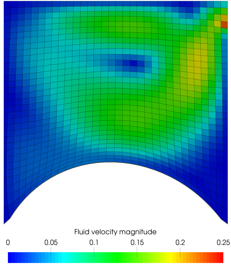
(b) Deformation of the flexible bottom and corresponding velocity field in $\text{\,}\mathrm{m}\text{/}\mathrm{s}$ at $t=$40\text{\,}\mathrm{s}\text{/}$$ simulated in the FV-FE framework.

Figure 2: Visualisations of the lid-driven cavity case.

The results obtained with the two frameworks are compared with each other as well as with data from literature in Figure 3, showing that the period of the oscillation matches well. Although there is some variation in the amplitude, the differences between the two frameworks are in line with the ones observed in literature.

Figure 3: Vertical displacement of the top center point of the flexible bottom wall as a function of time. The results of both frameworks are compared with each other as well as the results obtained by Mok [53] and Valdes [54].

5.1.2 Flexible tube case

The second case is the simulation of a pressure pulse travelling through a flexible tube [22]. In contrast to the lid-driven cavity case, this simulation is performed in three dimensions (3D). The tube has a length of $0.05\text{\,}\mathrm{m}\text{/}$, a radius of $0.005\text{\,}\mathrm{m}\text{/}$, and a wall thickness of $0.001\text{\,}\mathrm{m}\text{/}$. The material parameters are given in Table 2.

Table 2: Parameter values for the lid-driven cavity and flexible tube case.

	Flow parameter	Value	Solid parameter	Value
	$\rho^{f}$	$1\text{\,}\mathrm{kg}\text{/}{\mathrm{m}}^{3}$	$\rho_{s}$	$500\text{\,}\mathrm{kg}\text{/}{\mathrm{m}}^{3}$
Lid-driven cavity	$\mu^{f}$	$0.01\text{\,}\mathrm{Pa}\text{\,}\mathrm{s}\text{/}$	$E^{s}$	$250\text{\,}\mathrm{N}\text{/}{\mathrm{m}}^{2}$
			$\nu^{s}$	0.0
	$\rho^{f}$	$1000\text{\,}\mathrm{kg}\text{/}{\mathrm{m}}^{3}$	$\rho^{s}$	$1200\text{\,}\mathrm{kg}\text{/}{\mathrm{m}}^{3}$
Flexible tube	$\mu^{f}$	$0.003\text{\,}\mathrm{Pa}\text{\,}\mathrm{s}\text{/}$	$E^{s}$	$300\,000\text{\,}\mathrm{N}\text{/}{\mathrm{m}}^{2}$
			$\nu^{s}$	0.3

Both ends of the tube wall are clamped. At the inlet, a pressure value of $1333.2\text{\,}\mathrm{Pa}\text{/}$ is applied during the first $0.003\text{\,}\mathrm{s}\text{/}$, thereafter the pressure is $0\text{\,}\mathrm{Pa}\text{/}$. At the outlet, the pressure is fixed to $0\text{\,}\mathrm{Pa}\text{/}$. The total simulated time is $0.01\text{\,}\mathrm{s}\text{/}$, divided into 100 time steps of $0.0001\text{\,}\mathrm{s}\text{/}$. Figure 4 illustrates the pressure pulse travelling through the tube.

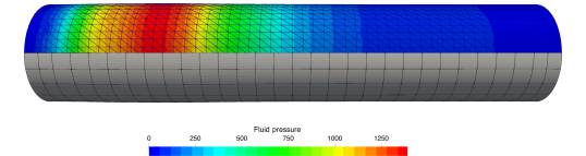
Figure 4: Flexible tube at $t=$0.004\text{\,}\mathrm{s}\text{/}$$ simulated in the FE-FE framework. The upper half shows the fluid pressure field in $\text{\,}\mathrm{Pa}\text{/}$ and the lower part illustrates the IGA shell structure.

As the purpose of this study is to investigate similar effects in both software frameworks rather than a quantitative comparison of the two, matching results are not strictly required. Nevertheless, Figure 5 compares the data obtained for both frameworks. Despite small quantitative differences, the two graphs are very similar.

Figure 5: Radial displacement plotted over the axial coordinate at $t=$0.004\text{\,}\mathrm{s}\text{/}$$ for both solver frameworks.

5.1.3 Settings of coupling and solvers

The FSI problems detailed above are solved with the quasi-Newton algorithm IQN-ILS [22]. For each problem, the reuse parameter $q$ is detailed in Table 3. Before constructing the approximate Jacobian, the linear dependencies in the stored residual data are removed by filtering [50]. Table 3 also contains the used filtering tolerances $\varepsilon^{fil}$, as well as the subproblem tolerances for the flow and solid solvers, $\varepsilon^{f}$ and $\varepsilon^{s}$, confer the discussion in Section 3. Table 4 shows that similar edge lengths have been aspired for both frameworks.

Table 3: Summary of the coupling and solver settings.

	$q$	$\varepsilon^{fil}$	$\varepsilon^{f}$	$\varepsilon^{s}$
Lid-driven cavity
FE-FE	3	$5$10-09$$	$1$10-09$$	$1$10-09$$
FV-FE	3	$1$10-09$$	$1$10-06$$	$1$10-09$$
Flexible tube
FE-FE	5	$1$10-12$$	$1$10-09$$	$1$10-09$$
FV-FE	5	$1$10-12$$	$1$10-07$$	$1$10-09$$

Table 4: Summary of discretization.

	Flow solver			Solid solver
	Cells/Elements	Nodes	DOFs	Elements	Control points/Nodes	DOFs
Lid-driven cavity
FE-FE	2 048	1 089	3 267	31	99	198
FV-FE	1 024	1 089	3 072	64	99	198
Flexible tube
FE-FE	35 986	7 195	28 780	600	800	4 800
FV-FE	7 200	7 913	28 800	780	800	4 800

5.2 Cost factors and regression

As explained in Section 4 the cost of a partitioned simulation is not determined by the number of coupling iterations alone, but instead also depends on the number of subproblem iterations. That is why the cost measure in Eq. (10) was introduced as a weighted sum of the iteration counts $N^{c}$, $N^{f}$, and $N^{s}$. The weights are given by a set of cost coefficients accounting for the data transfer as well as both a fixed and an iteration-dependent contribution of each solver call. While the values of these five cost factors are impossible to determine in general, they can be approximated for a specific case and framework using linear regression.

To do so, the total run time of each simulation is split into three parts: the time spent in the flow solver or flow time $t^{f}$, the time spent in the solid solver or solid time $t^{s}$, and finally the remainder, which will be called coupling time $t^{c}$. For each parameter study, i.e., a specific case and framework combination, the regression then uses the timings and iteration counts of all conducted runs as data set.

In the following, the calculations for the flexible tube case with FV-FE are used as example for the regression. The results themselves will be described in more detail in Section 5.3.

For the flow and solid time a multivariate linear regression is applied with two independent variables: the number of coupling iterations $N^{c}$ and the number of subproblem iterations $N^{f}$ or $N^{s}$. Neglecting any cost that occurs only once per simulation, a zero intercept is considered, such that the result of the regression is effectively a plane through the origin. As an example, Figure 6(a) shows this plane for the flow time of the tube case solved with the FV-FE framework, while Figure 6(b) projects the same data into a plot over the flow solver iterations.

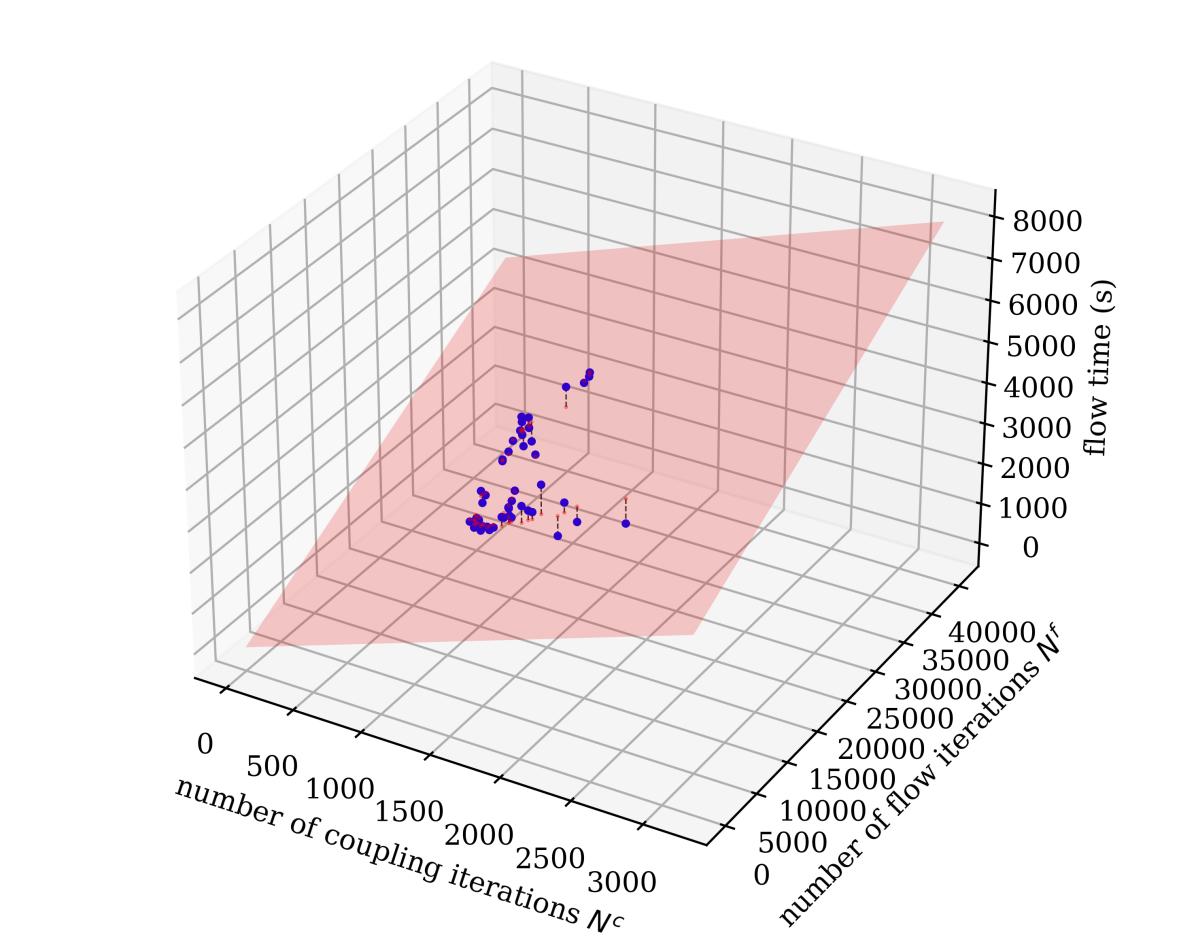
(a) Plane obtained with multivariate regression.

(b) Projection onto the flow time and $N_{f}$ plane.

Figure 6: Multi-variate linear regression of $t^{f}$ in function of $N^{c}$ and $N^{f}$ for the tube case with the FV-FE framework.

The accuracy of the fit is assessed by the relative root mean square error (RRMSE), which is calculated for the flow time as

$$\mathrm{RRMSE}=\sqrt{\frac{\sum^{m}\left\lvert t^{f}-(N^{c}\cdot C_{\text{fix}}^{f}+N^{f}\cdot C_{\text{iter}}^{f})\right\rvert^{2}}{\sum^{m}\left\lvert t^{f}\right\rvert^{2}}},$$ (12)

where $m$ is the number of calculations considered. For the flexible tube with FV-FE the RRMSE of the flow time regression is 7.43 %. This value shows that the regression is reasonably accurate. The remaining difference is caused by natural variation in run time due to the varying loading and clock speed of the processors as well as minor effects not considered in the model, like varying cost of solving the assembled matrix-vector system. Also, optimization actions taken by a solver behind the scenes such as load balancing or optimization of certain solver parameters, e.g., relaxation factors, contribute to the variations in run time. This is especially the case for the commercial FV solver in the FV-FE framework. For completeness, the RRMSE of the solid time regression is 3.44 %.

For the coupling time a linear regression analysis is performed with only one independent variable: the total number of coupling steps $N^{c}$. Again, a zero intercept is assumed, such that the result is a line through the origin. Figure 7 shows the line for the tube case solved with the FV-FE framework. The RRMSE value is 2.65 %, which is again low, indicating that the assumed proportionality between coupling iterations and coupling cost is accurate.

Figure 7: Linear regression of $t^{c}$ in function of $N^{c}$ for the tube case with the FV-FE framework.

As discussed in Section 4, all cost coefficients scaling with the number of coupling iterations can be combined into $\overline{C_{\text{}}}^{c}$. Plugging these coefficients into Eq. (10) gives a cost measure for the run time, which will be called the equivalent time. For the flexible tube case with FV-FE, the absolute value of the relative difference between the actual run time and the equivalent time is on average 3.80 % and never higher than 14.62 %. The first measure is referred to as the mean absolute percentage error (MAPE) and, analogously, the second is called the maximum absolute percentage error (maxAPE). These are defined as

$$\mathrm{MAPE}=\frac{1}{m}\sum^{m}\left\lvert\frac{t_{\text{simulation}}-C_{\text{simulation}}}{t_{\text{simulation}}}\right\rvert\quad\mathrm{and}\quad\mathrm{maxAPE}=\max_{m}\left(\left\lvert\frac{t_{\text{simulation}}-C_{\text{simulation}}}{t_{\text{simulation}}}\right\rvert\right).$$ (13)

For comparison, assuming that the total cost scales only with the coupling iterations as common in literature, i.e., setting $C_{\text{iteration}}^{f,s}=0$, the deviation increases to an average of 13.58 % and a maximum of 52.96 %. Figure 8 illustrates the difference between these measures and their error with respect to the actual cost of the simulation. Hence, the measure proposed in this work is not perfect, but definitely an improvement over the one predominant in literature.

Figure 8: Difference between the actual time, the equivalent time used here, and the cost measure considering a constant cost per coupling iteration for the flexible tube case with the FV-FE framework. Note that the equivalent time with constant cost per coupling iteration forms a line through the origin.

An additional benefit of this equivalent time is that it is not affected by the occurring variations in run time, as the random variations present in the actual run time are filtered out. For this reason, the equivalent time will be used as cost measure instead of the actual time from here on. Table 5 gives a summary of the cost factors and the differences between the actual and equivalent run time for the lid-driven cavity and flexible tube case with both frameworks

Table 5: Cost factors in seconds per corresponding iteration and difference between the actual and equivalent run time, expressed with the mean and maximum absolute percentage error.

	$C_{\text{fix}}^{f}$	$C_{\text{iter}}^{f}$	$C_{\text{fix}}^{s}$	$C_{\text{iter}}^{s}$	$C_{\text{}}^{c}$	$\overline{C_{\text{}}}^{c}$	MAPE	maxAPE
Lid-driven cavity
FE-FE	0.0208	0.0298	0.0002	0.0023	0.0004	0.0214	0.33 %	0.89 %
FV-FE	0.8985	0.0727	0.0243	0.0041	0.0218	0.9446	3.86 %	15.76 %
Flexible tube
FE-FE	0.6459	1.4756	0.0128	0.2076	0.1873	0.8460	0.22 %	0.58 %
FV-FE	1.1542	0.1068	0.1587	0.2510	0.0795	1.3924	3.80 %	14.62 %

The methodology explained in this section was illustrated by the flexible tube simulations with the FV-FE framework. Quality measures of the regression for other combinations of problems and frameworks are given in A.

5.3 Results of parameter study

The primary research question of this work is how the overall performance of the partitioned FSI algorithm is influenced by limiting the number of subproblem iterations per solver call. Towards this goal, simulations were run multiple times with varying values for $n_{max}^{f}$ and $n_{max}^{s}$. By virtue of the new convergence criterion, each of these runs solves the coupled problem up to the same tolerance. Two test cases investigated by two FSI software frameworks led to a total of four parameter studies. The following subsections present their results, focusing on how varying $n_{max}^{f}$ and $n_{max}^{s}$ influences different quantities and measures.

5.3.1 Iteration counts

One central aspect is the impact of the subproblem iterations per solver call on the three global iteration counts, i.e., the total number of coupling iterations $N^{c}$ as well as the total number of subproblem iterations of the flow and solid solver, $N^{f}$ and $N^{s}$, respectively. Therefore, Figure 9 and Figure 10 illustrate their dependence on $n_{max}^{f}$ and $n_{max}^{s}$ in three contour plots each. To increase the representativity of the examples, Figure 9 is based on the lid-driven cavity case simulated with the FV-FE framework, while Figure 10 visualizes the tube case for the FE-FE framework.

The overall trends observed for these two examples are in very good agreement. The biggest difference is that the plots obtained for the FV flow solver are more ’fine-grained’, since it relies on fixed-point rather than Newton steps, requiring more but typically less expensive iterations. The key findings of the three subplots are:

1. The number of coupling iterations clearly decreases when running more subproblem iterations per solver call, so that iterating to full convergence in every call yields the smallest $N^{c}$. This observation, in line with the reasoning of Section 4.2, is expected since the interface data fed back by the subproblem into the coupling loop is ensured to be as accurate as possible given the input data. The other way around, reducing $n_{max}^{f}$ and/or $n_{max}^{s}$ deteriorates the quality of the exchanged data fields, leading to more coupling iterations. This effect can even be severe enough to cause divergence of the coupling, as observed for the FV-FE framework in Figure 9 if $n_{max}^{f}<6$.

2. The main influence on the flow iterations is that the total number $N^{f}$ grows with $n_{max}^{f}$. This indicates that for increasing $n_{max}^{f}$, the increase in $N^{f}$ resulting from the additional subproblem iterations performed within each coupling step outweighs those saved due to the reduced number of coupling iterations, discussed in (a). Keeping $n_{max}^{f}$ fixed reveals a secondary trend: running more solid iterations per solver call decreases the total number of flow iterations. Again, this is explicable by the improved quality of the interface data that is passed back by the solid solver and serves as the fluid’s boundary condition.

3. The contour plot of the solid iterations and its characteristics are principally the transpose of those discussed for the flow iterations in (b): $N^{s}$ primarily depends on $n_{max}^{s}$, but is influenced by $n_{max}^{f}$ as well.

The contour plots of the two missing combinations, i.e., the lid-driven cavity with the FE-FE setup and the tube case simulated with the FV-FE solver framework, are omitted for the sake of conciseness. They show the same trends, which suggest the discussion above is to some extent general, in that the underlying effects are not very problem-dependent, or at least observable for typical FSI simulations.

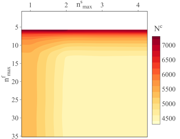
(a) Coupling iterations $N^{c}$.

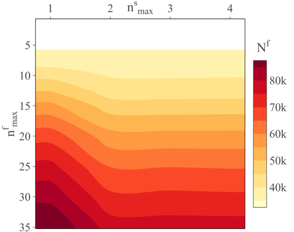
(b) Flow subproblem iterations $N^{f}$.

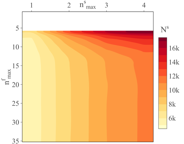
(c) Solid subproblem iterations $N^{s}$.

Figure 9: Different iteration counts plotted over $n_{max}^{f}$ and $n_{max}^{s}$ for the lid-driven cavity case simulated with the FV-FE framework.

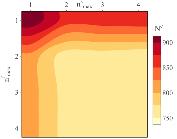
(a) Coupling iterations $N^{c}$.

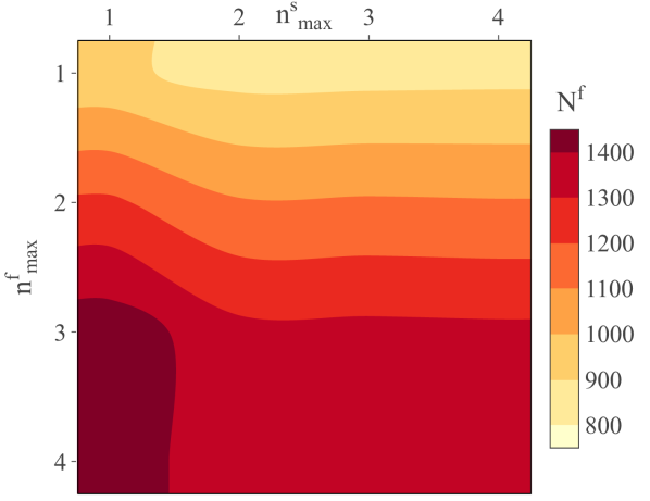
(b) Flow subproblem iterations $N^{f}$.

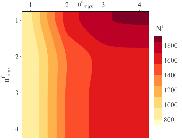
(c) Solid subproblem iterations $N^{s}$.

Figure 10: Different iteration counts plotted over $n_{max}^{f}$ and $n_{max}^{s}$ for the tube case simulated with the FE-FE framework.

5.3.2 Computational cost

Investigating the iteration counts $N^{c}$, $N^{f}$, $N^{s}$ is certainly of scientific interest, but in practice the most important quantity to consider is the simulation’s total run time, in this work represented by the equivalent time measure defined in Eq. (10). Since it is computed as a weighted sum of $N^{c}$, $N^{f}$, and $N^{s}$, all effects discussed in the previous section affect the equivalent time measure too. Their significance, however, is determined by the weighting factors, i.e., the cost of one coupling, flow, or solid iteration approximated by the regression model. Unlike the more general dependencies illustrated in Figure 9 and Figure 10, the equivalent time measure therefore strongly depends on other aspects such as the problem itself, the solver framework, the HPC architecture, and so on.

For the lid-driven cavity case, the parameter study of the two solver frameworks results in the contour plots depicted in Figure 11. To make them more comparable, the values are normalized by dividing through the equivalent time obtained for iterating each solver call to full convergence.

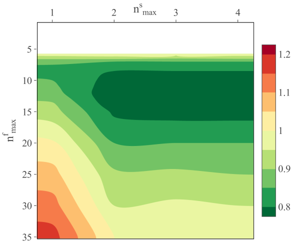
(a) FV-FE framework.

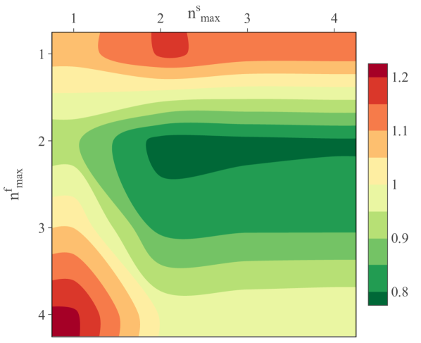
(b) FE-FE framework.

Figure 11: Contour plots of the equivalent time measure for the lid-driven cavity case, normalized with respect to the value obtained for full convergence.

The most striking observation is that, despite resulting from different solver frameworks run on different computer systems, the overall characteristics of the plots are very similar. The only major difference is found for the top part, i.e., for small values of $n_{max}^{f}$. While the FV-FE framework diverged for $n_{max}^{f}<6$ as discussed in the previous section, no lower bound is apparent for the FE-FE setup, as performing a single Newton iteration per flow solver call is already sufficient to ensure convergence. Nevertheless, the negative impact of $n_{max}^{f}=1$ on the stability leads to more coupling iterations and therefore higher computational cost.

Apart from this, the trends apparent in the two plots are in good agreement. They clearly show that the total run time is not minimized by iterating to full convergence in every solver call. Accordingly, the optima of the run time and the number of coupling iterations $N^{c}$ do not match. Moreover, the least efficient choice in both cases is to set $n_{max}^{s}=1$ and $n_{max}^{f}=\infty$. The area of lowest computational cost, on the other hand, is found for some mid-range values for both parameters, like $n_{max}^{f}=n_{max}^{s}=2$ for FE-FE or $n_{max}^{f}\approx 12$ and $n_{max}^{s}=2$ for the FV-FE framework. While further increasing $n_{max}^{f}$ reduces the efficiency significantly, adding more solid iterations in this case does not have a big impact, since solving the solid problem is much cheaper for both setups.

Although the most significant speed up with respect to full convergence in every solver call, i.e., $n_{max}^{f}=n_{max}^{s}=\infty$, is only about $22\%$, the parameter study of the lid-driven cavity case clearly shows that the number of subproblem iterations per solver call has a significant influence on the computational cost. In order to be efficient, an FSI solver framework should therefore take this impact into account.

Analogously to the discussion of the lid-driven cavity, Figure 12 illustrates the computational cost as a function of $n_{max}^{f}$ and $n_{max}^{s}$ for the flexible tube case. Undoubtedly, the difference between the two solver frameworks is more pronounced than in the previous figure. Nonetheless, the biggest difference is again observed for very small values of $n_{max}^{f}$. Like in the previous case, the FV flow solver requires a certain minimum number of subproblem iterations, here $n_{max}^{f}\gtrsim 8$, to prevent divergence. For the FE-FE framework, on the other hand, one Newton iteration per call is not only enough to converge, but in this case even results in the lowest computational cost. A likely explanation is that one Newton iteration is already accurate enough to yield similar results as in the green region observed in the FV-FE framework around $n_{max}^{f}\approx 12$, so that the part above with slightly slower convergence is never reached for the FE-FE setup. This reasoning is supported by the observation that for all FE flow solver calls of the parameter study, a maximum of three Newton iterations was enough to converge, indicating that Newton steps are a very effective method of handling the flow problem’s nonlinearity for this test case.

In both plots, increasing the number of flow iterations per solver call leads to a smooth yet significant growth in computational cost, while the solid iterations have a far lower impact. Furthermore, setting $n_{max}^{s}=1$ and $n_{max}^{f}=\infty$ is the most expensive choice for both frameworks. In that regard, the two plots are similar. However, this maximum is much more distinct in the FV-FE case than for FE-FE. Given the three contour plots in Figure 10, it is clear that the peak in the lower left corner stems from the flow solver’s cost. As the cost factors listed in Table 5 do not reveal the flow solver to be more expensive in the FV-FE framework relative to the other costs than for FE-FE, the difference is likely to be caused by a locally higher increase of the number of flow iterations $N^{f}$. This hypothesis is supported by the tables presented in B.

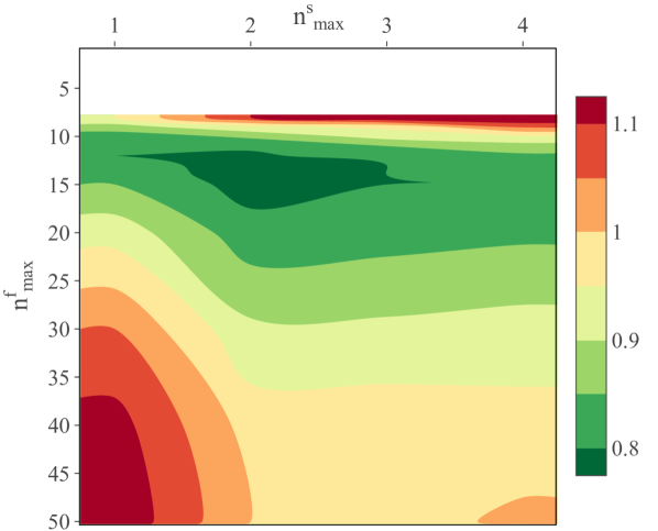
(a) FV-FE framework.

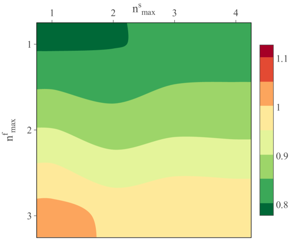
(b) FE-FE framework.

Figure 12: Contour plots of the equivalent time measure for the flexible tube case, normalized with respect to the value obtained for full convergence.

5.3.3 Further remarks

The contour plots discussed so far illustrated the most important trends and findings of the parameter studies. Further, B contains four tables, each corresponding to a particular parameter study, i.e., one test case and framework. They list the coupling, flow, and solid iterations as well as the relative equivalent times obtained for all runs belonging to that particular parameter study. The following additional observations and remarks are noteworthy:

• For both test cases, the FE-FE framework requires slightly fewer coupling iterations. This effect is caused by the different types of subproblem iterations. As the residual reduction is much more significant for a Newton step than it is for a fixed-point iteration, the first subproblem residual satisfying the convergence tolerance will typically be considerably lower for the FE solver than for its FV counterpart. Consequently, even for the same residual tolerance the FE results fed back into the coupling loop are on average more accurate. In line with the reasoning in Section 4.2 and Section 5.3.1, this leads to a lower $N^{c}$. The effect is further amplified since each solver call includes at least one subproblem iteration, i.e., a Newton step for FE or a fixed-point iteration for FV, even if the subproblem has already converged. While the higher number of coupling iterations is not problematic in itself, it results in a higher number of modes in the quasi-Newton coupling technique which risk to be (almost) linear dependent. This requires an efficient filtering technique, especially when the reuse parameter is high.

  Numerical experiments showed, however, that the higher number of coupling iterations observed for the FV solver can be countered by performing batches of fixed-point subproblem iterations, e.g., groups of ten, and checking convergence of the flow solver only after each batch.

• In literature, it is common to monitor the coupling’s convergence via the fixed-point residual of the interface displacement $\mathbf{r}^{k}$, defining either an absolute or relative tolerance. To give an idea of how strict the convergence criteria were chosen for the parameter study, Table 6 lists for all four studies both the average and maximum value of $\left\lVert\mathbf{r}^{k}\right\rVert_{2}$ and $\frac{\left\lVert\mathbf{r}^{k}\right\rVert_{2}}{\left\lVert\mathbf{d}^{k}\right\rVert_{2}}$, determined upon convergence for each time step.

• As explained in Remark 1, the convergence criterion is only exact if the IQN update increment vanishes. Therefore, Table 6 provides the average and maximum norm of the IQN increment norm at the end of a time step for all studies, confirming this minor aspect can safely be ignored in practice.

• By virtue of the new convergence criterion, all runs within a parameter study are converged up to the same tolerance. In this way, their results are virtually the same. To quantify the deviation, after each time step of each run in the parameter study, the computed interface displacement field $\mathbf{d}^{k}$ is compared to that obtained for iterating to full convergence in every call $\mathbf{d}^{k}_{ref}$, by evaluating

  $$\frac{\left\lVert\mathbf{d}^{k}-\mathbf{d}^{k}_{ref}\right\rVert_{2}}{\sqrt{n_{\Gamma}}}\leavevmode\nobreak\ ,$$ (14)

  where $n_{\Gamma}$ is the number of displacement degrees of freedom at the FSI interface. In its last two columns, Table 6 list the average and maximum values of this deviation for each study.

Table 6: Four different quantities that are evaluated after each time step of all simulations within the parameter study. The average and maximum value are reported. First, the norm of the fixed-point residual of the interface deformation $\mathbf{r}^{k}$ is given, followed by its relative magnitude with respect to the interface deformation $\mathbf{d}^{k}$. The third quantity is the norm of the IQN increment $\Delta\mathbf{\tilde{d}}^{k}_{IQN}$, while the last one evaluates the deviation from the results obtained for $n_{max}^{f}=n_{max}^{s}=\infty$.

	$\left\lVert\mathbf{r}^{k}\right\rVert_{2}$		$\frac{\left\lVert\mathbf{r}^{k}\right\rVert_{2}}{\left\lVert\mathbf{d}^{k}\right\rVert_{2}}$		$\left\lVert\Delta\mathbf{\tilde{d}}^{k}_{IQN}\right\rVert_{2}$		$\frac{\left\lVert\mathbf{d}^{k}-\mathbf{d}^{k}_{ref}\right\rVert_{2}}{\sqrt{n_{\Gamma}}}$
	Average	Max	Average	Max	Average	Max	Average	Max
Lid-driven cavity
FE-FE	$1.98$10-09$$	$6.58$10-07$$	$7.92$10-09$$	$7.84$10-06$$	$8.53$10-10$$	$5.80$10-07$$	$5.12$10-10$$	$7.36$10-9$$
FV-FE	$2.54$10-11$$	$9.04$10-10$$	$1.18$10-09$$	$1.49$10-06$$	$4.95$10-11$$	$9.14$10-10$$	$3.99$10-11$$	$1.93$10-10$$
Flexible Tube
FE-FE	$1.42$10-11$$	$1.90$10-10$$	$2.18$10-08$$	$1.10$10-06$$	$9.85$10-12$$	$1.56$10-10$$	$7.48$10-12$$	$2.63$10-11$$
FV-FE	$9.99$10-12$$	$2.33$10-10$$	$9.04$10-09$$	$5.44$10-07$$	$1.40$10-11$$	$2.56$10-10$$	$2.99$10-12$$	$8.34$10-12$$

The tables in B show that the gain in computational efficiency and the location of the optimum depend on the specific problem and the selected solvers. However, also the coupling technique and settings have a significant influence. To illustrate this, C presents two additional parameter studies for the flexible tube case with identical settings, but without reuse of data from past time steps in the IQN Jacobian approximation ($q$=0). For both tables, fully converging the subproblems in every call leads to the worst performance. The optimum is found by performing 1 Newton iteration in FE and around 8 fixed-point iterations in FV. Note that for these choices the computational time is approximately halved with respect to the reference.

5.3.4 Impact of cost factors

The parameter studies demonstrate that limiting the number of subproblem iterations per solver call has a significant influence on the computational cost of the partitioned simulation, and that this cost is accurately represented by the new equivalent time measure, which relies on a weighted sum of the iteration counts $N^{c}$, $N^{f}$, and $N^{s}$. Unfortunately, however, both weighting factors and iteration counts are case-specific: while the weighting factors refer to the cost of one iteration and hence in particular depend on the software framework and computer architecture, the iteration counts are influenced for example by the chosen solver tolerances and convergence criteria.

Nevertheless, Section 5.3.1 showed that these iteration counts follow rather general trends. Taking the iteration counts obtained in the parameter studies and artificially setting the cost factors $\overline{C_{\text{}}}^{c}$, $C_{\text{iter}}^{f}$, and $C_{\text{iter}}^{s}$, therefore allows to approximate the computational costs of different cost scenarios.

As an illustrative example, Figure 13 uses the iteration counts obtained for the cavity case simulated in the FV-FE framework to plot the computational cost resulting from different, artificially chosen cost factors, exemplarily imitating the effect of a cost-efficient flow solver (Figure 13b) or a very expensive data exchange (Figure 13c).

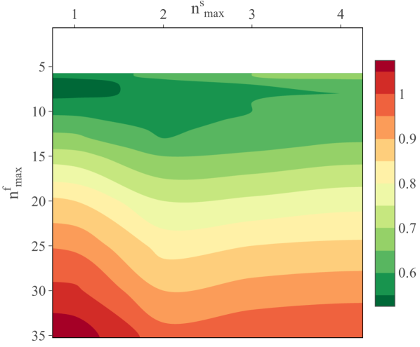
(a) $\overline{C_{\text{}}}^{c}=C_{\text{iter}}^{f}=C_{\text{iter}}^{s}=1$: running only a few subproblem iterations per call reduces the sum of iterations $N^{c}+N^{f}+N^{s}$, which is proportional to the overall cost for this scenario.

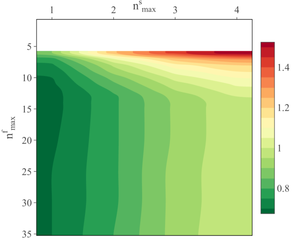
(b) $\overline{C_{\text{}}}^{c}=C_{\text{iter}}^{s}=1$, $C_{\text{iter}}^{f}=0.01$: in this scenario the flow iterations are very inexpensive, so that a high $n_{max}^{f}$ and a small $n_{max}^{s}$ are most efficient.

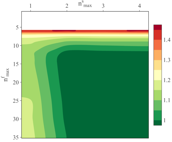
(c) $\overline{C_{\text{}}}^{c}=120$, $C_{\text{iter}}^{f}=C_{\text{iter}}^{s}=1$: if the cost per coupling step becomes dominant, it is best to run more subproblem iterations per call since it reduces $N^{c}$. Thus the potential speed-up decreases.

Figure 13: Contour plots of different cost distributions for the cavity case. The underlying approximate data is created by using the iteration counts obtained for the FV-FE framework and artificially setting the cost per coupling and subproblem iteration.

6 Conclusion

This work studies the influence of the nonlinear subproblem iterations on the computational cost of a partitioned scheme. Although the focus of this work is on partitioned algorithms for fluid-structure interaction problems, its findings are more widely applicable to any multi-field problem that is solved by coupling black-box solvers. While it is common in FSI literature to consider only the total number of coupling iterations, the subproblem iterations are demonstrated to be just as crucial for the overall computational cost. Consequently, converging in as few coupling iterations as possible does not necessarily minimize the run time of the partitioned simulation. In order to be efficient, a coupling algorithm instead should reduce the number of subproblem iterations in the flow and solid solver too. The cost measure proposed in this work therefore weights these conflicting objectives with the cost of one coupling, flow or solid iteration, respectively. Among other things, the cost factors depend on the considered problem, the employed solvers, and the computer hardware, making them very case-specific.

Nevertheless, this work sheds light on the relation between subproblem iterations and computational cost based on typical benchmark problems and common solver types by running multiple parameter studies. These studies systematically investigate how limiting the maximum number of subproblem iterations per solver call influences the total number of coupling, flow, and solid iterations as well as the required run time. To make sure all parameter sets yield the same solution fields, a new convergence criterion is proposed that relies solely on the convergence tolerances of the subproblem residuals, rather than introducing an own tolerance for the fixed-point residual as commonly done in literature This new way of assessing convergence can obviously also be applied in other FSI simulations.

The key finding of the parameter studies is that limiting the subproblem iterations per solver call cannot only reduce the total number of subproblem iterations, but also significantly lower the simulation’s overall computational cost. This raises the question of how many subproblem iterations per solver call yield the most efficient partitioned algorithm.

Unfortunately, this question is as non-trivial as it is important. Although a definite answer is yet to be found and is expected to be case-specific, the results discussed in this work demonstrate that iterating to full convergence in every solver call typically causes a computational overhead. Instead, running only a few subproblem iterations in each coupling step can be much more efficient. For the four parameter studies, the maximum reduction in computational cost was above $20\,\%$. Depending on the coupling technique, even higher savings are possible, as indicated by the studies without reuse of past time step data in the IQN for which the cost was almost halved. The ideal choice may be difficult or even impossible to determine a priori, but the results show that the optimum is rather flat. For example, limiting the Newton iterations per solver call to $2$ and the fixed-point iterations to $12$ led to a speed up of $12\,\%$ to $24\,\%$ for all test cases and frameworks investigated. While these performance gains might be no quantum leap, it should be noted that they come without any additional effort, cost, or code changes.

Furthermore, the limits imposed on the number of subproblem iterations per solver call were kept fixed here for the sake of cleaner parameter studies that are easier to interpret. Dynamically adapting $n_{max}^{f}$ and $n_{max}^{s}$ in a “smart” way, for example based on some quality measure for the coupling data, has the potential to further shorten the run time.

All in all, the primary goal of this work is to raise awareness of a gap in current literature on FSI and other coupled problems, concerning the number of subproblem iterations performed per solver call and how it influences the computational cost of a partitioned algorithm. In addition, this work lays the groundwork for potential future research bridging this gap.

Appendix A Additional regression measures

The regression method to obtain the cost factors is explained in Section 5.2, illustrated by the simulations of the flexible tube with the FV-FE. The accuracy of the various regressions for the other parameter studies is summarized in Table 7.

Besides the RRMSE, the absolute variant is also given, namely the root mean square error (RMSE)

$$\mathrm{RMSE}=\sqrt{\frac{\sum^{m}\left\lvert t^{f}-(N^{c}\cdot C_{\text{fix}}+N^{f}\cdot C_{\text{iter}})\right\rvert^{2}}{m}}.$$ (15)

Table 7: Quality measures for the coupling, flow, and solid regression for all parameters studies, as well as deviation between the actual and equivalent run times determined with the new measure $C_{\text{simulation}}$ and with the measure used in literature, i.e., only regarding the number of coupling iterations.

	Coupling		Flow		Solid		New equivalent time		Measure in literature
	RMSE	RRMSE	RMSE	RRMSE	RMSE	RRMSE	MAPE	maxAPE	MAPE	maxAPE
Lid-driven cavity
FE-FE	$0.2\text{\,}\mathrm{s}\text{/}$	7.88 %	$1.7\text{\,}\mathrm{s}\text{/}$	0.44 %	$0.3\text{\,}\mathrm{s}\text{/}$	1.26 %	0.33 %	0.89 %	22.77 %	34.32 %
FV-FE	$13.8\text{\,}\mathrm{s}\text{/}$	11.95 %	$468.7\text{\,}\mathrm{s}\text{/}$	5.60 %	$6.3\text{\,}\mathrm{s}\text{/}$	3.74 %	3.86 %	15.76 %	12.29 %	36.20 %
Flexible tube
FE-FE	$2.8\text{\,}\mathrm{s}\text{/}$	1.86 %	$7.3\text{\,}\mathrm{s}\text{/}$	0.32 %	$0.8\text{\,}\mathrm{s}\text{/}$	0.26 %	0.22 %	0.58 %	12.70 %	33.32 %
FV-FE	$2.7\text{\,}\mathrm{s}\text{/}$	2.65 %	$233.2\text{\,}\mathrm{s}\text{/}$	7.43 %	$27.7\text{\,}\mathrm{s}\text{/}$	3.44 %	3.80 %	14.62 %	13.58 %	52.69 %

Appendix B Additional results

To increase readability, the discussion, tables, and figures of Section 5 focused on one trend at a time. For the sake of completeness, this appendix groups all findings in a single table for each parameter study, listing the equivalent time measure, the number of coupling iterations, and the number of subproblem iterations for every run within a study. Table 8 and Table 9 list the results of the lid-driven cavity case for the FE-FE and FV-FE framework, respectively. Similarly, the flexible tube case with the FE-FE setup is covered by Table 10, and its FV-FE analogue by Table 11.

Table 8: Lid-driven cavity case with the FE-FE framework. The row and column header contain the maximal number of subproblem iterations for the flow and solid solver, $n_{max}^{f}$ and $n_{max}^{s}$, respectively. For each run, the normalized equivalent time is given, as well as the number of coupling iterations, flow solver iterations, and solid solver iterations.

		Newton iterations per coupling iteration - Structural solver
		1		2		3		$\infty$
Newton iterations per coupling iteration - Flow solver		1.07- 1.07 1.07 1.07 1.07	8554	1.15- 1.15 1.15 1.15 1.15	8876	1.12- 1.12 1.12 1.12 1.12	8542	1.12- 1.12 1.12 1.12 1.12	8499
	1	8554	8554	8876	17043	8542	18894	8499	19662
		0.91- 0.91 0.91 0.91 0.91	5066	0.78- 0.78 0.78 0.78 0.78	4304	0.78- 0.78 0.78 0.78 0.78	4293	0.79- 0.79 0.79 0.79 0.79	4299
	2	9014	5066	7470	7908	7452	9294	7473	10183
		1.05- 1.05 1.05 1.05 1.05	4985	0.83- 0.83 0.83 0.83 0.83	3989	0.84- 0.84 0.84 0.84 0.84	4014	0.84- 0.84 0.84 0.84 0.84	4002
	3	11098	4985	8489	7278	8515	8729	8458	9579
		1.21- 1.21 1.21 1.21 1.21	5004	0.99- 0.99 0.99 0.99 0.99	4007	0.99- 0.99 0.99 0.99 0.99	3982	1.00- 1.00 1.00 1.00 1.00	3974
	$\infty$	13487	5004	10853	7314	10761	8667	10786	9523

Table 9: Lid-driven cavity case with the FV-FE framework. The row and column header contain the maximal number of subproblem iterations for the flow and solid solver, $n_{max}^{f}$ and $n_{max}^{s}$, respectively. For each run, the normalized equivalent time is given, as well as the number of coupling iterations, flow solver iterations, and solid solver iterations. A missing value indicates that the coupling did not converge.

		Newton iterations per coupling iteration - Structural solver
		1		2		3		$\infty$
Fixed-point iterations per coupling iteration - Flow solver		– - - - -	-	– - - - -	-	– - - - -	-	– - - - -	-
	5	-	-	-	-	-	-	-	-
		0.96- 0.96 0.96 0.96 0.96	7209	0.97- 0.97 0.97 0.97 0.97	7204	0.95- 0.95 0.95 0.95 0.95	7111	0.96- 0.96 0.96 0.96 0.96	7176
	6	37477	7209	37581	12900	36929	16148	37399	17802
		0.86- 0.86 0.86 0.86 0.86	6218	0.85- 0.85 0.85 0.85 0.85	6126	0.85- 0.85 0.85 0.85 0.85	6132	0.85- 0.85 0.85 0.85 0.85	6138
	7	36473	6218	35965	10865	36001	13791	36068	15110
		0.84- 0.84 0.84 0.84 0.84	5882	0.81- 0.81 0.81 0.81 0.81	5613	0.81- 0.81 0.81 0.81 0.81	5618	0.81- 0.81 0.81 0.81 0.81	5608
	8	38449	5882	36629	9926	36706	12648	36590	13896
		0.84- 0.84 0.84 0.84 0.84	5692	0.79- 0.79 0.79 0.79 0.79	5328	0.79- 0.79 0.79 0.79 0.79	5318	0.79- 0.79 0.79 0.79 0.79	5310
	9	40841	5692	38382	9443	38163	11991	38127	13234
		0.85- 0.85 0.85 0.85 0.85	5581	0.78- 0.78 0.78 0.78 0.78	5091	0.78- 0.78 0.78 0.78 0.78	5075	0.78- 0.78 0.78 0.78 0.78	5103
	10	43394	5581	39559	8943	39430	11354	39631	12683
		0.86- 0.86 0.86 0.86 0.86	5485	0.77- 0.77 0.77 0.77 0.77	4906	0.77- 0.77 0.77 0.77 0.77	4885	0.77- 0.77 0.77 0.77 0.77	4888
	11	45919	5485	40814	8613	40662	10865	40715	12124
		0.87- 0.87 0.87 0.87 0.87	5398	0.76- 0.76 0.76 0.76 0.76	4706	0.76- 0.76 0.76 0.76 0.76	4718	0.76- 0.76 0.76 0.76 0.76	4720
	12	48329	5398	41953	8279	42020	10519	41978	11790
		0.89- 0.89 0.89 0.89 0.89	5387	0.76- 0.76 0.76 0.76 0.76	4607	0.76- 0.76 0.76 0.76 0.76	4602	0.76- 0.76 0.76 0.76 0.76	4588
	13	51042	5387	43364	8056	43320	10201	43319	11447
		0.91- 0.91 0.91 0.91 0.91	5373	0.77- 0.77 0.77 0.77 0.77	4566	0.77- 0.77 0.77 0.77 0.77	4545	0.77- 0.77 0.77 0.77 0.77	4546
	14	53842	5373	45288	7982	45168	10091	45386	11354
		0.92- 0.92 0.92 0.92 0.92	5352	0.79- 0.79 0.79 0.79 0.79	4558	0.78- 0.78 0.78 0.78 0.78	4534	0.78- 0.78 0.78 0.78 0.78	4534
	15	56336	5352	47478	7966	47241	10068	47344	11351
		1.01- 1.01 1.01 1.01 1.01	5349	0.85- 0.85 0.85 0.85 0.85	4519	0.85- 0.85 0.85 0.85 0.85	4487	0.85- 0.85 0.85 0.85 0.85	4500
	20	67992	5349	56902	7903	56645	9958	56739	11219
		1.07- 1.07 1.07 1.07 1.07	5357	0.91- 0.91 0.91 0.91 0.91	4511	0.91- 0.91 0.91 0.91 0.91	4498	0.90- 0.90 0.90 0.90 0.90	4483
	25	76627	5357	64779	7896	64833	9994	64530	11213
		1.12- 1.12 1.12 1.12 1.12	5345	0.95- 0.95 0.95 0.95 0.95	4499	0.96- 0.96 0.96 0.96 0.96	4503	0.95- 0.95 0.95 0.95 0.95	4491
	30	83527	5345	71215	7886	71336	9997	71008	11211
		1.17- 1.17 1.17 1.17 1.17	5348	1.00- 1.00 1.00 1.00 1.00	4523	1.00- 1.00 1.00 1.00 1.00	4492	1.00- 1.00 1.00 1.00 1.00	4509
	$\infty$	89966	5348	77618	7922	77344	9983	77272	11221

Table 10: Flexible tube case with the FE-FE framework. The row and column header contain the maximal number of subproblem iterations for the flow and solid solver, $n_{max}^{f}$ and $n_{max}^{s}$, respectively. For each run, the normalized equivalent time is given, as well as the number of coupling iterations, flow solver iterations, and solid solver iterations.

		Newton iterations per coupling iteration - Structural solver
		1		2		3		$\infty$
Newton iterations per coupling iteration - Flow solver		0.79- 0.79 0.79 0.79 0.79	920	0.80- 0.80 0.80 0.80 0.80	863	0.82- 0.82 0.82 0.82 0.82	866	0.82- 0.82 0.82 0.82 0.82	870
	1	920	920	863	1626	866	1840	870	1879
		0.91- 0.91 0.91 0.91 0.91	815	0.88- 0.88 0.88 0.88 0.88	757	0.89- 0.89 0.89 0.89 0.89	758	0.89- 0.89 0.89 0.89 0.89	752
	2	1218	815	1109	1414	1112	1623	1107	1642
		1.03- 1.03 1.03 1.03 1.03	811	0.99- 0.99 0.99 0.99 0.99	763	1.00- 1.00 1.00 1.00 1.00	761	1.00- 1.00 1.00 1.00 1.00	755
	3	1461	811	1328	1426	1326	1628	1321	1647
		1.03- 1.03 1.03 1.03 1.03	811	0.99- 0.99 0.99 0.99 0.99	763	1.00- 1.00 1.00 1.00 1.00	761	1.00- 1.00 1.00 1.00 1.00	755
	$\infty$	1461	811	1328	1426	1326	1628	1321	1647

Table 11: Flexible tube case with the FV-FE framework. The row and column header contain the maximal number of subproblem iterations for the flow and solid solver, $n_{max}^{f}$ and $n_{max}^{s}$, respectively. For each run, the normalized equivalent time is given, as well as the number of coupling iterations, flow solver iterations, and solid solver iterations. A missing value indicates that the coupling did not converge.

		Newton iterations per coupling iteration - Structural solver
		1		2		3		$\infty$
Fixed-point iterations per coupling iteration - Flow solver		1.14- 1.14 1.14 1.14 1.14	2135	– - - - -	-	– - - - -	-	– - - - -	-
	7	13567	2135	-	-	-	-	-	-
		0.95- 0.95 0.95 0.95 0.95	1716	1.10- 1.10 1.10 1.10 1.10	1814	– - - - -	-	1.16- 1.16 1.16 1.16 1.16	1749
	8	12120	1716	13006	3471	-	-	12438	5006
		0.88- 0.88 0.88 0.88 0.88	1544	0.94- 0.94 0.94 0.94 0.94	1517	0.96- 0.96 0.96 0.96 0.96	1481	1.06- 1.06 1.06 1.06 1.06	1586
	9	11896	1544	11838	2847	11581	3492	12381	4358
		0.82- 0.82 0.82 0.82 0.82	1400	0.86- 0.86 0.86 0.86 0.86	1348	0.92- 0.92 0.92 0.92 0.92	1387	0.94- 0.94 0.94 0.94 0.94	1385
	10	11758	1400	11351	2488	11722	3225	11667	3646
		0.81- 0.81 0.81 0.81 0.81	1355	0.81- 0.81 0.81 0.81 0.81	1245	0.85- 0.85 0.85 0.85 0.85	1254	0.88- 0.88 0.88 0.88 0.88	1279
	11	12242	1355	11281	2291	11430	2865	11542	3275
		0.80- 0.80 0.80 0.80 0.80	1299	0.79- 0.79 0.79 0.79 0.79	1189	0.83- 0.83 0.83 0.83 0.83	1201	0.84- 0.84 0.84 0.84 0.84	1196
	12	12701	1299	11457	2175	11614	2695	11584	3055
		0.82- 0.82 0.82 0.82 0.82	1299	0.78- 0.78 0.78 0.78 0.78	1154	0.80- 0.80 0.80 0.80 0.80	1143	0.81- 0.81 0.81 0.81 0.81	1133
	13	13455	1299	11767	2093	11717	2552	11621	2835
		0.84- 0.84 0.84 0.84 0.84	1289	0.77- 0.77 0.77 0.77 0.77	1114	0.80- 0.80 0.80 0.80 0.80	1114	0.83- 0.83 0.83 0.83 0.83	1137
	14	14155	1289	12101	2036	12085	2462	12278	2852
		0.85- 0.85 0.85 0.85 0.85	1278	0.78- 0.78 0.78 0.78 0.78	1104	0.80- 0.80 0.80 0.80 0.80	1101	0.80- 0.80 0.80 0.80 0.80	1076
	15	14872	1278	12604	2013	12540	2430	12156	2658
		0.93- 0.93 0.93 0.93 0.93	1264	0.82- 0.82 0.82 0.82 0.82	1062	0.83- 0.83 0.83 0.83 0.83	1049	0.84- 0.84 0.84 0.84 0.84	1046
	20	18399	1264	14898	1914	14672	2280	14534	2570
		1.05- 1.05 1.05 1.05 1.05	1255	0.91- 0.91 0.91 0.91 0.91	1050	0.91- 0.91 0.91 0.91 0.91	1031	0.92- 0.92 0.92 0.92 0.92	1033
	30	23462	1255	18756	1873	18217	2233	18154	2518
		1.12- 1.12 1.12 1.12 1.12	1264	0.98- 0.98 0.98 0.98 0.98	1069	0.98- 0.98 0.98 0.98 0.98	1043	0.97- 0.97 0.97 0.97 0.97	1010
	40	26140	1264	21584	1922	21056	2265	20296	2486
		1.14- 1.14 1.14 1.14 1.14	1273	1.00- 1.00 1.00 1.00 1.00	1064	0.98- 0.98 0.98 0.98 0.98	1021	1.01- 1.01 1.01 1.01 1.01	1037
	50	26768	1273	22083	1932	21210	2206	21368	2564
		1.14- 1.14 1.14 1.14 1.14	1263	0.99- 0.99 0.99 0.99 0.99	1052	0.98- 0.98 0.98 0.98 0.98	1030	1.00- 1.00 1.00 1.00 1.00	1028
	$\infty$	27089	1263	21898	1892	21292	2206	21282	2543

Appendix C Additional results without reuse

Table 12 and Table 13 present two additional parameter studies for the FE-FE and FV-FE framework, respectively, simulating the flexible tube case with identical settings, but without reuse of data from past time steps in the IQN Jacobian approximation ($q$=0).

Table 12: Flexible tube case simulated with the FE-FE framework, but without reusing past data in the IQN Jacobian approximation. The formatting is the same as in the previous tables. The cost factors determined by the regression model for this parameter study are, in seconds, $C_{\text{iter}}^{f}=0.2177$, $C_{\text{iter}}^{s}=0.2253$ and $\overline{C_{\text{}}}^{c}=0.1620$.

		Newton iterations per coupling iteration - Structural solver
		1		2		3		$\infty$
Newton iterations per coupling iteration - Flow solver		0.53- 0.53 0.53 0.53 0.53	1465	0.69- 0.69 0.69 0.69 0.69	1417	0.76- 0.76 0.76 0.76 0.76	1417	0.77- 0.77 0.77 0.77 0.77	1417
	1	1465	1465	1417	2734	1417	3330	1417	3362
		0.67- 0.67 0.67 0.67 0.67	1463	0.82- 0.82 0.82 0.82 0.82	1416	0.90- 0.90 0.90 0.90 0.90	1416	0.91- 0.91 0.91 0.91 0.91	1416
	2	2573	1463	2479	2732	2479	3328	2479	3360
		0.77- 0.77 0.77 0.77 0.77	1463	0.92- 0.92 0.92 0.92 0.92	1416	1.00- 1.00 1.00 1.00 1.00	1416	1.00- 1.00 1.00 1.00 1.00	1416
	3	3318	1463	3206	2732	3206	3328	3206	3360
		0.77- 0.77 0.77 0.77 0.77	1463	0.92- 0.92 0.92 0.92 0.92	1416	1.00- 1.00 1.00 1.00 1.00	1416	1.00- 1.00 1.00 1.00 1.00	1416
	$\infty$	3318	1463	3206	2732	3206	3328	3206	3360

Table 13: Flexible tube case simulated with the FV-FE framework, but without reusing past data in the IQN Jacobian approximation. The formatting is the same as in the previous tables. The cost factors determined by the regression model for this parameter study are, in seconds, $C_{\text{iter}}^{f}=0.1139$, $C_{\text{iter}}^{s}=0.2410$, and $\overline{C_{\text{}}}^{c}=1.2825$.

		Newton iterations per coupling iteration - Structural solver
		1		2		3		$\infty$
Fixed-point iterations per coupling iteration - Flow solver		0.54- 0.54 0.54 0.54 0.54	2077	0.61- 0.61 0.61 0.61 0.61	2120	0.61- 0.61 0.61 0.61 0.61	2044	0.64- 0.64 0.64 0.64 0.64	2060
	5	9641	2077	9815	3970	9444	4721	9511	5286
		0.50- 0.50 0.50 0.50 0.50	1834	0.55- 0.55 0.55 0.55 0.55	1827	0.57- 0.57 0.57 0.57 0.57	1827	0.59- 0.59 0.59 0.59 0.59	1828
	6	10097	1834	10052	3427	10050	4299	10045	4892
		0.50- 0.50 0.50 0.50 0.50	1746	0.54- 0.54 0.54 0.54 0.54	1757	0.57- 0.57 0.57 0.57 0.57	1763	0.59- 0.59 0.59 0.59 0.59	1756
	7	10960	1746	10973	3261	10986	4101	10965	4715
		0.50- 0.50 0.50 0.50 0.50	1691	0.54- 0.54 0.54 0.54 0.54	1681	0.57- 0.57 0.57 0.57 0.57	1685	0.59- 0.59 0.59 0.59 0.59	1685
	8	11881	1691	11844	3101	11880	3928	11899	4582
		0.50- 0.50 0.50 0.50 0.50	1638	0.54- 0.54 0.54 0.54 0.54	1610	0.57- 0.57 0.57 0.57 0.57	1620	0.59- 0.59 0.59 0.59 0.59	1633
	9	12889	1638	12767	2994	12811	3807	12841	4490
		0.51- 0.51 0.51 0.51 0.51	1595	0.55- 0.55 0.55 0.55 0.55	1578	0.57- 0.57 0.57 0.57 0.57	1583	0.59- 0.59 0.59 0.59 0.59	1593
	10	13941	1595	13729	2923	13758	3727	13772	4418
		0.52- 0.52 0.52 0.52 0.52	1579	0.55- 0.55 0.55 0.55 0.55	1555	0.58- 0.58 0.58 0.58 0.58	1559	0.60- 0.60 0.60 0.60 0.60	1559
	11	15046	1579	14713	2865	14741	3672	14741	4360
		0.54- 0.54 0.54 0.54 0.54	1572	0.56- 0.56 0.56 0.56 0.56	1531	0.59- 0.59 0.59 0.59 0.59	1523	0.61- 0.61 0.61 0.61 0.61	1520
	12	16166	1572	15756	2820	15747	3608	15745	4302
		0.55- 0.55 0.55 0.55 0.55	1564	0.58- 0.58 0.58 0.58 0.58	1520	0.60- 0.60 0.60 0.60 0.60	1515	0.62- 0.62 0.62 0.62 0.62	1515
	13	17309	1564	16836	2787	16814	3577	16815	4280
		0.57- 0.57 0.57 0.57 0.57	1562	0.59- 0.59 0.59 0.59 0.59	1511	0.61- 0.61 0.61 0.61 0.61	1509	0.63- 0.63 0.63 0.63 0.63	1508
	14	18463	1562	17905	2767	17872	3565	17863	4267
		0.59- 0.59 0.59 0.59 0.59	1563	0.60- 0.60 0.60 0.60 0.60	1502	0.63- 0.63 0.63 0.63 0.63	1500	0.65- 0.65 0.65 0.65 0.65	1500
	15	19615	1563	18969	2746	18915	3541	18914	4246
		0.67- 0.67 0.67 0.67 0.67	1564	0.67- 0.67 0.67 0.67 0.67	1483	0.70- 0.70 0.70 0.70 0.70	1474	0.72- 0.72 0.72 0.72 0.72	1470
	20	25033	1564	24210	2684	24124	3471	24107	4178
		0.80- 0.80 0.80 0.80 0.80	1564	0.81- 0.81 0.81 0.81 0.81	1479	0.83- 0.83 0.83 0.83 0.83	1472	0.85- 0.85 0.85 0.85 0.85	1472
	30	34388	1564	33540	2676	33450	3461	33440	4170
		0.90- 0.90 0.90 0.90 0.90	1564	0.91- 0.91 0.91 0.91 0.91	1479	0.93- 0.93 0.93 0.93 0.93	1472	0.95- 0.95 0.95 0.95 0.95	1472
	40	41504	1564	40657	2675	40565	3461	40556	4170
		0.93- 0.93 0.93 0.93 0.93	1564	0.94- 0.94 0.94 0.94 0.94	1479	0.96- 0.96 0.96 0.96 0.96	1472	0.99- 0.99 0.99 0.99 0.99	1472
	50	43672	1564	42838	2675	42749	3461	42741	4170
		0.93- 0.93 0.93 0.93 0.93	1564	0.96- 0.96 0.96 0.96 0.96	1479	0.98- 0.98 0.98 0.98 0.98	1472	1.00- 1.00 1.00 1.00 1.00	1472
	$\infty$	43677	1564	43793	2675	43704	3461	43697	4170

References

- [1] C. A. Felippa, K.-C. Park, C. Farhat, Partitioned analysis of coupled mechanical systems, Computer Methods in Applied Mechanics and Engineering 190 (24-25) (2001) 3247–3270. doi:10.1016/s0045-7825(00)00391-1.
- [2] P. Causin, J.-F. Gerbeau, F. Nobile, Added-mass effect in the design of partitioned algorithms for fluid-structure problems, Computer Methods in Applied Mechanics and Engineering 194 (42–44) (2005) 4506–4527. doi:10.1016/j.cma.2004.12.005.
- [3] C. Förster, W. Wall, E. Ramm, Artificial added mass instabilities in sequential staggered coupling of nonlinear structures and incompressible viscous flows, Computer Methods in Applied Mechanics and Engineering 196 (7) (2007) 1278–1293. doi:10.1016/j.cma.2006.09.002.
- [4] H. van Brummelen, Added mass effects of compressible and incompressible flows in fluid-structure interaction, Journal of Applied Mechanics 76 (2) (2009) 021206–1–7. doi:10.1115/1.3059565.
- [5] L. Formaggia, J.-F. Gerbeau, F. Nobile, A. Quarteroni, On the coupling of 3D and 1D Navier-Stokes equations for flow problems in compliant vessels, Computer Methods in Applied Mechanics and Engineering 191 (6–7) (2001) 561–582. doi:10.1016/s0045-7825(01)00302-4.
- [6] J. Vierendeels, K. Dumont, E. Dick, P. Verdonck, Analysis and stabilization of fluid-structure interaction algorithm for rigid-body motion, American Institute of Aeronautics and Astronautics Journal 43 (12) (2005) 2549–2557. doi:10.2514/1.3660.
- [7] S. Badia, F. Nobile, C. Vergara, Fluid-structure partitioned procedures based on Robin transmission conditions, Journal of Computational Physics 227 (14) (2008) 7027–7051. doi:10.1016/j.jcp.2008.04.006.
- [8] M. M. Joosten, W. G. Dettmer, D. Perić, Analysis of the block Gauss-Seidel solution procedure for a strongly coupled model problem with reference to fluid-structure interaction, International Journal for Numerical Methods in Engineering 78 (7) (2009) 757–778. doi:10.1002/nme.2503.
- [9] D. P. Mok, W. A. Wall, E. Ramm, Accelerated iterative substructuring schemes for instationary fluid-structure interaction, in: K.-J. Bathe (Ed.), Computational Fluid and Solid Mechanics, Elsevier, 2001, pp. 1325–1328. doi:10.1016/b978-008043944-0/50907-0.
- [10] D. P. Mok, W. A. Wall, Partitioned analysis schemes for the transient interaction of incompressible flows and nonlinear flexible structures, in: K. Schweizerhof, W. A. Wall, K.-U. Bletzinger (Eds.), Trends in computational structural mechanics, CIMNE, Barcelona, Spain, 2001, pp. 688–698.
- [11] U. Küttler, W. Wall, Fixed-point fluid-structure interaction solvers with dynamic relaxation, Computational Mechanics 43 (1) (2008) 61–72. doi:10.1007/s00466-008-0255-5.
- [12] J. Degroote, P. Bruggeman, R. Haelterman, J. Vierendeels, Stability of a coupling technique for partitioned solvers in FSI applications, Computers & Structures 86 (23–24) (2008) 2224–2234. doi:10.1016/j.compstruc.2008.05.005.
- [13] J. Degroote, S. Annerel, J. Vierendeels, Stability analysis of Gauss-Seidel iterations in a partitioned simulation of fluid-structure interaction, Computers & Structures 88 (5–6) (2010) 263–271. doi:10.1016/j.compstruc.2009.09.003.
- [14] N. Delaissé, T. Demeester, D. Fauconnier, J. Degroote, Comparison of different quasi-Newton techniques for coupling of black box solvers, in: F. Chinesta, R. Abgrall, O. Allix, M. Kaliske (Eds.), 14th WCCM & ECCOMAS Congress 2020, Proceedings, CIMNE, Paris, France, 2021, pp. 1–12. doi:10.23967/wccm-eccomas.2020.088.
- [15] N. Delaissé, T. Demeester, R. Haelterman, J. Degroote, Quasi-Newton methods for partitioned simulation of fluid-structure interaction reviewed in the generalized Broyden framework, Archives of Computational Methods in Engineering In press (2023).
- [16] K.-J. Bathe, Finite Element Procedures, Prentice Hall, Upper Saddle River, New Jersey, 1996.
- [17] F. Nobile, C. Vergara, An effective fluid-structure interaction formulation for vascular dynamics by generalized Robin conditions, SIAM Journal on Scientific Computing 30 (2) (2008) 731–763. doi:10.1137/060678439.
- [18] T. Spenke, M. Make, N. Hosters, A Robin-Neumann scheme with quasi-Newton acceleration for partitioned fluid-structure interaction, International Journal for Numerical Methods in Engineering 124 (4) (2023) 979–997. doi:10.1002/nme.7151.
- [19] T. Spenke, N. Hosters, M. Behr, A multi-vector interface quasi-Newton method with linear complexity for partitioned fluid–structure interaction, Computer Methods in Applied Mechanics and Engineering 361 (2020) 112810. doi:10.1016/j.cma.2019.112810.
- [20] N. Delaissé, T. Demeester, D. Fauconnier, J. Degroote, Surrogate-based acceleration of quasi-Newton techniques for fluid-structure interaction simulations, Computers & Structures 260 (2022) 106720. doi:10.1016/j.compstruc.2021.106720.
- [21] F. Lindner, M. Mehl, K. Scheufele, B. Uekermann, A comparison of various quasi-Newton schemes for partitioned fluid-structure interaction, in: B. Schrefler, E. Oñate, M. Papadrakakis (Eds.), 6th International Conference on Computational Methods for Coupled Problems in Science and Engineering, CIMNE, 2015, pp. 477–488.
- [22] J. Degroote, K.-J. Bathe, J. Vierendeels, Performance of a new partitioned procedure versus a monolithic procedure in fluid–structure interaction, Computers & Structures 87 (11-12) (2009) 793–801. doi:10.1016/j.compstruc.2008.11.013.
- [23] L. Pauli, M. Behr, On stabilized space-time FEM for anisotropic meshes: incompressible Navier-Stokes equations and applications to blood flow in medical devices, International Journal for Numerical Methods in Fluids 85 (3) (2017) 189–209. doi:10.1002/fld.4378.
- [24] J. Donea, A. Huerta, Finite Element Methods for Flow Problems, John Wiley & Sons, 2003. doi:10.1002/0470013826.
- [25] D. Forti, L. Dedè, Semi-implicit BDF time discretization of the Navier–Stokes equations with VMS-LES modeling in a high performance computing framework, Computers & Fluids 117 (2015) 168–182. doi:10.1016/j.compfluid.2015.05.011.
- [26] A. A. Johnson, T. E. Tezduyar, Mesh update strategies in parallel finite element computations of flow problems with moving boundaries and interfaces, Computer Methods in Applied Mechanics and Engineering 119 (1-2) (1994) 73–94. doi:10.1016/0045-7825(94)00077-8.
- [27] M. Behr, F. Abraham, Free-surface flow simulations in the presence of inclined walls, Computer Methods in Applied Mechanics and Engineering 191 (47-48) (2002) 5467–5483. doi:10.1016/S0045-7825(02)00444-9.
- [28] C. Förster, W. A. Wall, E. Ramm, On the geometric conservation law in transient flow calculations on deforming domains, International Journal for Numerical Methods in Fluids 50 (12) (2006) 1369–1379. doi:10.1002/fld.1093.
- [29] T. J. Hughes, J. A. Cottrell, Y. Bazilevs, Isogeometric analysis: CAD, finite elements, NURBS, exact geometry and mesh refinement, Computer Methods in Applied Mechanics and Engineering 194 (39-41) (2005) 4135–4195. doi:10.1016/j.cma.2004.10.008.
- [30] J. A. Cottrell, T. J. Hughes, Y. Bazilevs, Isogeometric Analysis: Toward Integration of CAD and FEA, John Wiley & Sons, 2009. doi:10.1002/9780470749081.ch7.
- [31] J. Chung, G. Hulbert, A time integration algorithm for structural dynamics with improved numerical dissipation: the generalized- method, Journal of Applied Mechanics 60 (1993) 371. doi:10.1115/1.2900803.
- [32] S. Erlicher, L. Bonaventura, O. S. Bursi, The analysis of the generalized- method for non-linear dynamic problems, Computational Mechanics 28 (2) (2002) 83–104. doi:10.1007/s00466-001-0273-z.
- [33] N. Hosters, Spline-based methods for fluid-structure interaction, Ph.D. thesis, RWTH Aachen University, Aachen, Germany (2018). doi:10.18154/RWTH-2018-223770.
- [34] M. K. P. Make, Spline-based methods for aerothermoelastic problems, Ph.D. thesis, RWTH Aachen University, Aachen, Germany (2021). doi:10.18154/RWTH-2021-03363.
- [35] ANSYS, Inc., ANSYS Fluent Theory Guide, 2019R3 (Aug. 2019).
- [36] T. J. Barth, D. Jespersen, The design and application of upwind schemes on unstructured meshes, in: American Institute of Aeronautics and Astronautics (Ed.), 27th Aerospace Sciences Meeting, American Institute of Aeronautics and Astronautics, 1989. doi:10.2514/6.1989-366.
- [37] C. M. Rhie, W. L. Chow, Numerical study of the turbulent flow past an airfoil with trailing edge separation, American Institute of Aeronautics and Astronautics Journal 21 (11) (1983) 1525–1532. doi:10.2514/3.8284.
- [38] J. Batina, Unsteady Euler airfoil solutions using unstructured dynamic meshes, American Institute of Aeronautics and Astronautics Journal 28 (8) (1990) 1381–1388. doi:10.2514/3.25229.
- [39] V. M. Ferrándiz, P. Bucher, R. Rossi, R. Zorrilla, J. Cotela, J. Maria, M. A. Celigueta, G. Casas, Kratosmultiphysics/kratos: Release 9.2, Zenodo (2022). doi:10.5281/ZENODO.3234644.
- [40] M. Lombardi, N. Parolini, A. Quarteroni, Radial basis functions for inter-grid interpolation and mesh motion in FSI problems, Computer Methods in Applied Mechanics and Engineering 256 (2013) 117–131. doi:10.1016/j.cma.2012.12.019.
- [41] J.-D. Müller, Essentials of Computational Fluid Dynamics, Taylor & Francis Group, 2015.
- [42] H. Versteeg, W. Malalasekera, An Introduction to Computational Fluid Dynamics, Longman Scientific & Technical, Essex, England, 1995.
- [43] J. Ferziger, M. Peric, Computational Methods for Fluid Dynamics, Springer Berlin Heidelberg, 2002.
- [44] O. C. Zienkiewicz, R. L. Taylor, J. Z. Zhu, The Finite Element Method: Its Basis and Fundamentals, Elsevier, 2013. doi:10.1016/C2009-0-24909-9.
- [45] O. C. Zienkiewicz, R. L. Taylor, The Finite Element Method for Solid and Structural Mechanics, Elsevier, 2005.
- [46] J. N. Reddy, Introduction to the Finite Element Method, McGraw-Hill Education, 2019.
- [47] J. N. Reddy, D. K. Gartling, The Finite Element Method in Heat Transfer and Fluid Dynamics, CRC press, 2010.
- [48] Y. Saad, M. H. Schultz, GMRES: A generalized minimal residual algorithm for solving nonsymmetric linear systems, SIAM Journal on Scientific and Statistical Computing 7 (3) (1986) 856–869. doi:10.1137/0907058.
- [49] K. Stüben, A review of algebraic multigrid, Journal of Computational and Applied Mathematics 128 (1-2) (2001) 281–309. doi:10.1016/s0377-0427(00)00516-1.
- [50] J. Degroote, Partitioned simulation of fluid-structure interaction, Archives of Computational Methods in Engineering 20 (3) (2013) 185–238. doi:10.1007/s11831-013-9085-5.
- [51] K. Scheufele, M. Mehl, Robust multisecant quasi-Newton variants for parallel fluid-structure simulations—and other multiphysics applications, SIAM Journal on Scientific Computing 39 (5) (2017) 404–433. doi:10.1137/16M1082020.
- [52] R. Schussnig, D. R. Pacheco, T.-P. Fries, Efficient split-step schemes for fluid–structure interaction involving incompressible generalised Newtonian flows, Computers & Structures 260 (2022) 106718. doi:10.1016/j.compstruc.2021.106718.
- [53] D. P. Mok, Partitionierte Lösungsansätze in der Strukturdynamik und der Fluid-Struktur-Interaktion, Ph.D. thesis, Universität Stuttgart, Stuttgart, Germany (2001). doi:10.18419/OPUS-147.
- [54] G. Valdés, Nonlinear analysis of orthotropic membrane and shell structures including fluid-structure interaction, Ph.D. thesis, Universitat Politècnica de Catalunya, Barcelona, Spain (2007).