A multi-wavelength view of the multiple activity cycles of $\epsilon$ Eridani

$\epsilon$ Eridani is a highly active young K2 star with an activity cycle of about three years established using Ca ii H& K line index measurements (S_MWO). This relatively short cycle has been demonstrated to be consistent with X-ray and magnetic flux measurements. Recent work suggested a change in the cyclic behaviour. Here we report new X-ray flux and S_MWO measurements and also include S_MWO measurements from the historical Mount Wilson program. This results in an observational time baseline of over 50 years for the S_MWO data and of over 7 years in X-rays. Moreover, we include Ca ii infrared triplet (IRT) index measurements (S${}_{\rm Ca\leavevmode\nobreak\ IRT}$) from 2013-2022 in our study. With the extended X-ray data set, we can now detect the short cycle for the first time using a periodogram analysis. Near-simultaneous S_MWO data and X-ray fluxes, which are offset by 20 days at most, are moderately strongly correlated when only the lowest activity state (concerning short-term variability) is considered in both diagnostics. In the S_MWO data, we find strong evidence for a much longer cycle of about 34 years and an 11-year cycle instead of the formerly proposed $12$-year cycle in addition to the known 3-year cycle. The superposition of the three periods naturally explains the recent drop in S_MWO measurements. The two shorter cycles are also detected in the S${}_{\rm Ca\leavevmode\nobreak\ IRT}$ data, although the activity cycles exhibit lower amplitudes in the S${}_{\rm Ca\leavevmode\nobreak\ IRT}$ than in the S_MWO data. Finally, the rotation period of $\epsilon$ Eri can be found more frequently in the S_MWO as well as in the S${}_{\rm Ca\leavevmode\nobreak\ IRT}$ data for times near the minimum of the long cycle. This may be explained by a scenario in which the filling factor for magnetically active regions near cycle maximum is too high to allow for notable short-term variations.

1 Introduction

$\epsilon$ Eridani ($\epsilon$ Eri; HD 22049) is a K2 V star at a distance of 3.2 pc (Bailer-Jones et al. 2021). It is known to host one planet with a semi-major axis of 3.4 AU and a planetary candidate at 40 AU (Hatzes et al. 2000; Quillen & Thorndike 2002). The latter was inferred by its imprint on the morphology of the dust ring around $\epsilon$ Eri. The stellar age was determined by Barnes (2007) to be 440 Myr from gyrochronology, while Marsden et al. (2015) found an age of 480 Myr from its chromospheric activity level. The chromospheric activity of $\epsilon$ Eri has been studied extensively, starting with measurements from the the Mount Wilson S-index (S_MWO) program in 1968 (Wilson 1978), which provided a purely instrumental index covering the emission cores of the Ca ii H&K lines.

The Mount Wilson HK project discovered activity cycles for many F- to K-type stars (Baliunas et al. 1995) and also determined a rotation period of 11.10$\pm$0.03 days and an activity cycle of approximately five years for $\epsilon$ Eri (Gray & Baliunas 1995). Later, Fröhlich (2007) revealed differential rotation with two rotation periods measured at $P_{\rm rot}$=11.35 days and $P_{\rm rot}$=11.555 days. Moreover, Metcalfe et al. (2013) reanalysed the Mount Wilson data and also included data from the Small and Moderate Aperture Research Telescope System (SMARTS) southern HK project. The authors proposed two cycles in $\epsilon$ Eri, one with 2.95$\pm$0.03 yr, the other with 12.7$\pm$0.3 yr length. With these properties, $\epsilon$ Eri is one of the youngest stars with a known activity cycle. Metcalfe et al. (2013) also found peaks between 3 and 7 years in their periodogram analysis, which they discarded, and a peak at 20-35 years, which they excluded because this time span is similar to the length of the adopted data set.

The 3-year cycle was also studied by other means. For example, Scalia et al. (2018) found that the integrated longitudinal magnetic field shows a period comparable to the 3-year S_MWO cycle. In a more detailed analysis, Jeffers et al. (2022) found that the net axis-symmetric component of the toroidal magnetic field correlates with the 12-year calcium cycle modulated by the short S_MWO cycle. Moreover, $\epsilon$ Eri is one of the few stars for which a cycle was detected in X-rays. Using XMM-Newton observations, Coffaro et al. (2020) found the X-ray variations to be consistent with the 3-year S_MWO cycle. Based on modelling of $\epsilon$ Eri X-ray spectra with observations of our Sun, treating it in the framework of the-Sun-as-an-Xray-star (see references in Coffaro et al. (2020)), they found that the X-ray cycle is characterised by changes in the filling factor of magnetically active structures ranging between 60% to 90% from minimum to maximum activity level. This high coronal filling factor throughout the whole activity cycle also explains the low amplitude of the X-ray cycle compared to that of the Sun. X-ray cycle maxima also exhibit high filling factors of flaring regions. This finding, indirectly inferred from comparison with solar data treated with the Sun-as-an-Xray-star technique, is consistent with the fact that resolved flares in the X-ray light curves are predominantly found near cycle maxima. Nevertheless, Burton & MacGregor (2021) found a flare at millimeter wavelengths in data taken by the ALMA instrument at the beginning of 2015. In this time, the activity of $\epsilon$ Eri was in a minimum state.

Coffaro et al. (2020) also noted that S_MWO data collected with the TIGRE telescope (Schmitt et al. 2014) seems to indicate a change in the cycle behaviour in observations since 2018, as the expected 2019 maximum was not seen in the S_MWO data, but only in the X-ray measurements. The component of the magnetic field measured by Jeffers et al. (2022) also indicates lower values in 2019, which Jeffers et al. (2022) interpreted as being caused by the superposition of the magnetic field components of the 3- and 12-year cycles.

Here we extend the time-series of the S_MWO data from the work by Coffaro et al. (2020) both to older (using the Mount Wilson program data) and to newer data up to February 2022 (from the TIGRE telescope). This collection of more than 50 years of S_MWO observations, corresponding to dozens of the $3$-year cycles, allows us to search for multiple and especially very long cycles for $\epsilon$ Eri, such as those that were presented for other stars, for example, by Brandenburg et al. (2017). It also enables us to study cycle length variations, which are well known for the Sun (Hathaway 2015; Ivanov 2021), in another star. Dynamo theory can explain cyclic activity behaviour as such, but different shapes or lengths of individual cycles are not well understood or even constrained yet because it is difficult to monitor the stars for a sufficiently long time.

We intend to study the ongoing transition in chromospheric activity by adding more data to the S_MWO measurements as well as activity indices defined for the Ca ii infrared triplet (IRT) lines measured with the TIGRE telescope. We also want to extend the studies of coronal activity by adding the latest X-ray data observed with XMM-Newton.

2 Observations and data analysis

$\epsilon$ Eri has been monitored with different instruments in optical spectroscopy with a total time baseline of more than $50$ years and for 7 years in the X-ray waveband.

In the following, we present the Ca ii $S_{\rm MWO}$ data acquired by different ground-based observatories (Sect. 2.1) and the X-ray monitoring campaign (Sect. 2.2) with the XMM-Newton satellite. For the X-ray data, we also include an analysis of the short-term variations of the coronal flux due to flares. These variations potentially contaminate long-term variations and should therefore be excluded from a determination of the activity cycle.

2.1 Optical data

The $S_{\rm MWO}$ values used here originate from different observatories; the oldest are from the Mount Wilson program itself. Further optical spectroscopic observations for $\epsilon$ Eri were obtained within the California Planet Search (CPS) program at the Keck and Lick Observatories (Isaacson & Fischer 2010), with the Solar-Stellar Spectrograph located at the Lowell Observatory, and with the SMARTS instrument at the Cerro Tololo Interamerican Observatory. From these data, $S_{\rm MWO}$ values were derived and already published in Coffaro et al. (2020), where a more detailed description of these data can also be found. Coffaro et al. (2020) also presented $S_{\rm MWO}$ values from the TIGRE telescope located in Guanajato, Mexico (Schmitt et al. 2014; González-Pérez et al. 2022). The optical monitoring with the TIGRE telescope of $\epsilon$ Eri is still ongoing, and we present here data until mid February 2022. Moreover, we include here activity indices $S_{\rm CaIRT}$ that were calculated from the spectra of the TIGRE telesope for the Ca ii IRT lines as described by Mittag et al. (2017). These lines are located at 8498, 8542, and 8662 Å,  and the respective line and continuum wavebands used for the calculation of $S_{\rm CaIRT}$ can be found in Mittag et al. (2017). These lines can be used for chromospheric activity studies, as was shown for example by their correlation with Ca ii H&K in flux-flux relations for F to M dwarfs studied by Martínez-Arnáiz et al. (2011).

Timing information of all Ca II data can be found in Table 1. Since especially the Mount Wilson program included multiple observations per night (usually three; but single nights have $>$200 observations), we computed the mean of these observations. We therefore have one (mean) $S_{\rm MWO}$ measurement per night, which leaves us with 675 Mount Wilson program measurements and a total of 1578 measurements taken between 1967 and 2022. From these, we clipped three apparent outliers with one S_MWO$<0.36$ and two measurements $>0.63$. One of the two high S_MWO values is from the CPS program, and the other is an individual measurement from the Mount Wilson program. Both are likely caused by flaring activity. Since the data from the Mount Wilson and SMARTS programs do not have errors assigned and because part of the Lowell observatory data have exceptionally low errors, we used an error of 3% for all data because this is the median error of the TIGRE data. Of this whole data set, we considered the two subsets separately, namely the Mount Wilson data and the TIGRE data. These are separated in time by about 20 years. When we considered only the TIGRE data, the errors obtained from the pipeline were used.

We excluded $S_{\rm CaIRT}$ data from between 30 November 2014 and 16 May 2015 because a different camera was used for the red spectrograph arm of TIGRE during that period.

Table 1: Basic information about the Ca ii observations.

Telescope	No.	JD first	JD last	covered
	spectra	[day]	[day]	years
Mount Wilson	4336	2439786.8	2449771.6	1967-1995
CPS	168	2452267.7	2455415.1	2001-2010
SMARTS	146	2454334.7	2456324.0	2007-2013
Lowell Obs.	267	2449258.9	2458154.5	1993-2018
TIGRE	322	2456518.9	2459624.6	2013-2022
all data
1 day binning	1578
TIGRE Ca ii IRT	303	2456518.9	2459624.6
excluded times		2456992.0	2457159.0

2.2 X-ray observations

At X-ray wavelengths, a monitoring campaign started in August 2015 (PI: B.Stelzer) using the XMM-Newton satellite. It consists of snapshots with durations between 7.6 and 21.5  ks, repeated roughly every six months. Prior to this campaign, $\epsilon$ Eri had been observed twice with XMM-Newton, in January 2003 and February 2015 (PIs: B. Aschenbach and K. France). XMM-Newton observed $\epsilon$ Eri employing all X-ray telescopes on board. Hence, we have EPIC (pn+MOS) and RGS data products. For this work, we made use of EPIC/pn data. EPIC/MOS provides a lower signal-to-noise ratio and does not yield additional information for our study. The analysis of the RGS data is deferred to a future work. As $\epsilon$ Eri is a bright star ($m_{V}\sim 3$), the Optical Monitor on board of XMM-Newton cannot be used.

The first three years of monitoring (2015-2018), plus the 2003 and 2015 archival data, in total nine observations, were presented and analysed by Coffaro et al. (2020). These authors discovered the X-ray cycle of $\epsilon$ Eri. After 2018, the X-ray monitoring continued until January 2022, providing seven new observations. We follow the approach described by Coffaro et al. (2020) and justified above that we extracted data from the EPIC/pn detector alone. The observing log of all available XMM-Newton pointing observations is given in Table 2. For later reference throughout this article, we define in col. 1 a running number for each observation following chronological order.

Table 2: X-ray observations with XMM-Newton.

Obs.	Date	Rev.	Science Mode	Exposure time
no.			(EPIC/pn)	[ksec]
1	2003-01-19	0570	Full window	13.4
2	2015-02-02	2775	Large window	20.0
3	2015-07-19	2858	Small window	8.0
4	2016-02-01	2957	Small window	9.3
5	2016-07-19	3042	Small window	11.0
6	2017-01-16	3133	Small window	7.6
7	2017-08-26	3244	Small window	10.3
8	2018-01-16	3316	Small window	8.0
9	2018-07-20	3408	Small window	21.5
10	2019-01-19	3500	Small window	18.4
11	2019-07-19	3591	Small window	8.8
12	2020-01-19	3683	Small window	7.9
13	2020-07-22	3776	Small window	9.9
14	2021-01-17	3866	Small window	8.9
15	2021-08-07	3967	Small window	8.0
16	2022-01-17	4049	Small window	13.9

2.3 Analysis of XMM-Newton data

The focus of this work is to study the long-term variability of $\epsilon$ Eri. However, this requires an assessment of short-term variations that could modify the time-averaged flux of each snapshot observation. In order to obtain reliable flux measurements for comparison to the optical data, we identified flaring episodes and excluded them from the further data analysis. This process is described in the following.

2.3.1 Short-term variability in EPIC/pn light curves

EPIC/pn data were extracted with the software called Science Analysis System (SAS; version 17.0.0). The standard SAS tools were applied to filter event lists of each observation and produce the images, and also to extract the light curve and spectrum of $\epsilon$ Eri for each individual observation. Then we identified flaring states using a timing analysis and the hardening of the X-ray spectrum, which is caused by higher temperatures during flares.

First, the EPIC/pn light curves of $\epsilon$ Eri were extracted in the $0.2-2.0$ keV energy band, and they were binned with a bin size of $300$ s. Following the approach of Coffaro et al. (2020), we searched for short-term variability in each light curve with the software R and its library changepoint (Killick & Eckley 2014). Through this analysis, Coffaro et al. (2020) found that four out of nine observations to display short-term variability. For the seven new observations, short-term variability was identified in five light curves. In Fig. 7 we show all variable light curves. The segments are identified by changepoint and are drawn as dash-dotted black lines. For comparison, we also show the light curves with a constant count rate in Fig. 8. They represent the lowest count rates, that is, the most quiescent observations of $\epsilon$ Eri .

This short-term variability might be related to flares. To search for evidence of heating episodes, we generated light curves of the hardness ratio (HR) for observations that the software R flagged as variable. The HR is calculated as

$$HR=\dfrac{C_{h}-C_{s}}{C_{h}+C_{s}},$$ (1)

where $C_{h}$ and $C_{s}$ are the count rates in a hard and a soft energy band, respectively. We chose the energy range $0.2-1.0$ keV as soft band and $1.0-2.0$ keV as hard band. The HR light curves of each observation are shown in the bottom panels of each plot in Fig. 7. In each of these HR light curves, we looked for variability with the software R, analogously to the treatment of the light curves outlined above. The corresponding segments are indicated with the dash-dotted green lines in each bottom panel.

2.3.2 Spectral analysis of EPIC/pn data

We analysed the EPIC/pn spectra of each observation with the software xspec. We chose a 3-T APEC model with global metal abundances frozen at $0.3\ Z_{\odot}$. We did not include photoelectric absorption because $\epsilon$ Eri is very nearby, thus no interstellar absorption is expected. The best-fitting model provides three emission measures (EM) and three thermal energy components (kT), and the results are given in Table 3 for all observations presented here for the first time, while an analogous table is found in Coffaro et al. (2020) for the data up to 2018.

Table 3: Best-fit spectral parameters of all XMM-Newton EPIC/pn observation of $\epsilon$ Eri   that are presented here for the first time

. Obs $kT_{1}$ $kT_{2}$ $kT_{3}$ $logEM_{1}$ $logEM_{2}$ $logEM_{3}$ Flux $L_{\rm X}$ $T_{\rm av}$ $\overline{\chi}^{2}$ No. (0.2-2 keV) (0.2-2 keV) [keV] [keV] [keV] [cm^-3] [cm^-3] [cm^-3] [10^-11 erg cm^-2 s^-1] [10²⁸ erg s^-1] [keV] 10 0.12 $\pm$ 0.01 0.31 $\pm$0.01 0.71 $\pm$0.02 50.70 $\pm$0.09 50.93 $\pm$0.02 50.34 $\pm$0.06 1.25 $\pm$0.02 1.54$\pm$ 0.01 0.31$\pm$ 0.02 1.39 11 0.21 $\pm$ 0.04 0.43 $\pm$0.07 0.87 $\pm$0.07 50.87 $\pm$0.05 50.80 $\pm$0.07 50.81 $\pm$0.04 1.85 $\pm$0.03 2.27$\pm$ 0.04 0.49$\pm$ 0.03 1.01 12 0.14 $\pm$ 0.02 0.32 $\pm$0.02 0.68 $\pm$0.05 50.63 $\pm$0.11 50.97 $\pm$0.05 50.34 $\pm$0.08 1.28 $\pm$0.03 1.57$\pm$ 0.04 0.32$\pm$ 0.02 0.95 13 0.17 $\pm$ 0.03 0.33 $\pm$0.02 0.72 $\pm$0.03 50.68 $\pm$0.15 50.93 $\pm$0.12 50.57 $\pm$0.06 1.50 $\pm$0.03 1.84$\pm$ 0.04 0.37$\pm$ 0.02 0.98 14 0.17 $\pm$ 0.03 0.34 $\pm$0.02 0.75 $\pm$0.02 50.71 $\pm$0.07 51.02 $\pm$0.07 50.68 $\pm$0.05 1.80 $\pm$0.03 2.21$\pm$ 0.04 0.40$\pm$ 0.02 1.26 15 0.14 $\pm$ 0.02 0.32 $\pm$0.02 0.71 $\pm$0.04 50.67 $\pm$0.10 50.94 $\pm$0.08 50.37 $\pm$0.08 1.30 $\pm$0.03 1.59$\pm$ 0.04 0.33$\pm$ 0.02 0.90 16 0.15 $\pm$ 0.02 0.31 $\pm$ 0.04 0.79 $\pm$ 0.02 50.62 $\pm$ 0.08 50.91 $\pm$ 0.12 50.52 $\pm$ 0.05 1.34 $\pm$0.02 1.65$\pm$ 0.03 0.37$\pm$ 0.02 1.26

We calculated the EM weighted average thermal energy as

$$kT_{\rm av}=\dfrac{\sum_{i}kT_{i}\cdot EM_{i}}{\sum_{i}EM_{i}},$$ (2)

where $i=1,2,3$ is the index for each spectral component. We also calculated the X-ray fluxes observed at Earth ($F_{\rm x}$) in the soft energy band $0.2-2.0$ keV, and the X-ray luminosity $L_{\rm X}$. In Table 2 we report the $kT_{\rm av}$ and $F_{\rm X}$ values obtained from the spectral fitting. The errors given there are the statistical errors from the fitting process, which represent the 95% confidence level. The variability in the X-ray light curves of the individual observations indicates larger flux changes, however. Following Sanz-Forcada et al. (2019), we therefore used the standard deviation of the flux variations within a given light curve as the flux error for the timing analysis.

For each of the observations that were flagged as variable by the software R, the same spectral analysis as described above for the time-average of each observation was repeated for two time intervals. That is, we extracted two separate spectra, one spectrum referring to the quiescent state of the observation (the segment with the lowest count rate in the light curve), and another within the flare-like event (the segment identified by R with the highest count rate). In Table 4 we report the $kT_{\rm av}$ and $F_{\rm X}$ values of the best fit to these different activity states. An increase in the average plasma thermal energy is found for all flare-like time intervals, but in most cases, it is only marginally significant.

The changes in coronal flux and average thermal energy within each observation derived from the time-resolved spectral fitting are visualised in Fig. 1, where for each of the observations with a variable light curve, we display the ratio of the highest and lowest brightness state. The errors were calculated with the error propagation for the values for quiescent and flaring part given in Table 4.

Fig. 1 shows that $kT_{\rm av}$ significantly changed within the observations of July 2016 (observation 5), August 2018 (observation 9), August 2019 (observation 11), and January 2022 (observation 16). Out of these, observations 5, 11, and 16 also show variations of the HR that are compatible with the variability identified in the count rate (see Fig. 7). We conclude that all four observations are likely to be affected by flare-like activity.

Based on this variability analysis, we defined three different X-ray flux data sets for the subsequent analysis. X-ray flux set I contains only average fluxes from Table 2 of Coffaro et al. (2020) and Table 3, which means that no correction was applied for possible flaring activity. In X-ray flux set II, the average fluxes for all observations that are flagged as variable are replaced by the quiescent fluxes from Table 4. In X-ray flux set III, only the four measurements with significant thermal energy variation described above are replaced by the respective quiescent fluxes.

Table 4: X-ray flux and emission-weighted average thermal energy for quiescent and flaring time-intervals of the EPIC/pn observations of $\epsilon$ Eri that show variability (see text in Sect. 2.3.2)

. No. Obs $F_{\rm X}$ $kT_{\rm av}$ obs. [$10^{-11}$ erg cm^-2 s^-1] [keV] Quiescent Flaring Quiescent Flaring 1 02/2003 $1.23\pm 0.01$ $1.47\pm 0.02$ $0.36\pm 0.02$ $0.40\pm 0.05$ 5 07/2016 $1.76\pm 0.03$ $2.03\pm 0.02$ $0.39\pm 0.03$ $0.46\pm 0.06$ 8 01/2018 $1.80\pm 0.04$ $2.05\pm 0.02$ $0.42\pm 0.09$ $0.44\pm 0.05$ 9 08/2018 $1.86\pm 0.02$ $2.37\pm 0.02$ $0.38\pm 0.02$ $0.47\pm 0.03$ 10 01/2019 $1.20\pm 0.01$ $1.33\pm 0.03$ $0.32\pm 0.02$ $0.34\pm 0.08$ 11 08/2019 $1.56\pm 0.02$ $2.08\pm 0.02$ $0.41\pm 0.05$ $0.53\pm 0.04$ 13 08/2020 $1.44\pm 0.02$ $1.73\pm 0.04$ $0.36\pm 0.03$ $0.36\pm 0.06$ 14 01/2021 $1.71\pm 0.02$ $1.83\pm 0.03$ $0.39\pm 0.03$ $0.42\pm 0.07$ 16 01/2022 $1.22\pm 0.01$ $1.52\pm 0.02$ $0.33\pm 0.02$ $0.44\pm 0.09$
Notes: $F_{\rm X}$ and $kT_{\rm av}$ were derived from spectral fitting of EPIC/pn data for the light curves flagged as variable with the changepoint analysis; see Sect. 2.3.2 for the definition of the two brightness states. Errors are 95% confidence levels computed with the XSPEC error command.

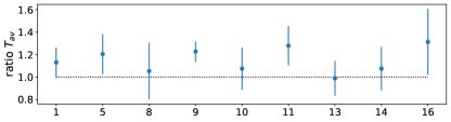
Figure 1: Parameter ratio of the flaring and quiescent state for all EPIC/pn light curves flagged variable with the changepoint analysis; see Sect. 2.3.2 for the definition of the two brightness states and Table 4 for the numbering of the observations.

3 Results

3.1 Correlation of the data

First, we investigated the correlation between the optical indices, S_MWO  and S${}_{\rm Ca\leavevmode\nobreak\ IRT}$, and the X-ray fluxes. These correlations have been examined on a statistical basis in large stellar samples for example by Martínez-Arnáiz et al. (2011); Stelzer et al. (2013); Martin et al. (2017); Mittag et al. (2017).

In these studies, a single data point (mostly not contemporaneous for the different activity indicators that are compared) was usually available for a given star. Differently from this work, we searched for correlations between optical and X-ray activity diagnostics in a large data set for a single star.

For the optical indices, we only considered the TIGRE data because S${}_{\rm Ca\leavevmode\nobreak\ IRT}$ measurements were obtained only for these data. We compare the S_MWO  and S${}_{\rm Ca\leavevmode\nobreak\ IRT}$ data in Fig. 2, where a correlation is apparent. We list all formal correlation coefficients in Table 5. The Pearson correlation coefficient $r$ shows a very good correlation between these four line indices with $r>0.85$ and a probability $p$ that the correlation were zero of $p<10^{-75}$ for all line combinations, except for S_MWO to S${}_{\rm Ca\leavevmode\nobreak\ IRT}$ for the $8542\,{\rm\AA}$ line, which only has $r=0.81$.

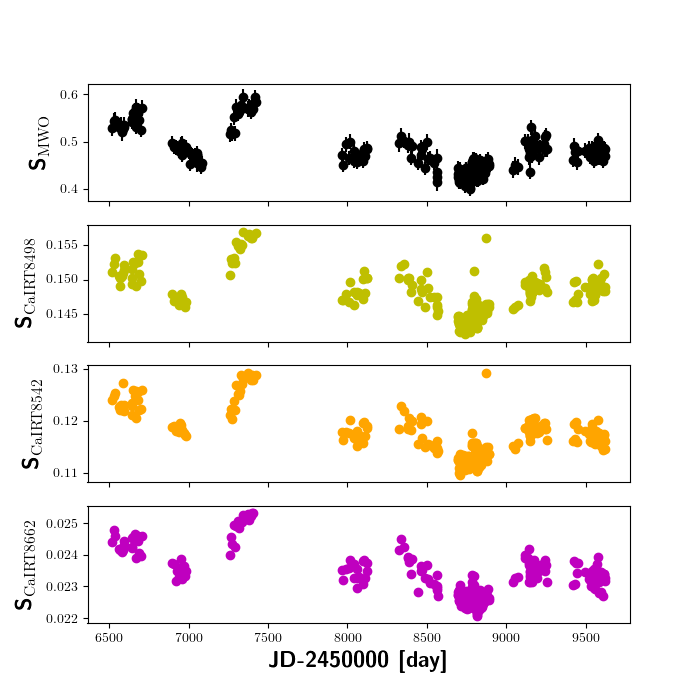
Figure 2: Time series of chromospheric indicators. TIGRE S_MWO  (black dots; top) and S${}_{\rm Ca\leavevmode\nobreak\ IRT}$  data (yellow, orange, and magenta dots corresponding to the lines at 8498, 8542, and 8662 Å;  lower three panels).

Table 5: Pearson correlation coefficients for different chromospheric and coronal activity indicators.

indicators	$r$	$p$
SMWO – S${}_{\rm Ca\leavevmode\nobreak\ IRT}$8498	0.85	1.3$\cdot 10^{-91}$
SMWO – S${}_{\rm Ca\leavevmode\nobreak\ IRT}$8542	0.81	1.3$\cdot 10^{-75}$
SMWO – S${}_{\rm Ca\leavevmode\nobreak\ IRT}$8662	0.88	8.3$\cdot 10^{-104}$
S${}_{\rm Ca\leavevmode\nobreak\ IRT}$8498 – S${}_{\rm Ca\leavevmode\nobreak\ IRT}$8542	0.92	3.4$\cdot 10^{-129}$
S${}_{\rm Ca\leavevmode\nobreak\ IRT}$8498 – S${}_{\rm Ca\leavevmode\nobreak\ IRT}$8662	0.90	3.6$\cdot 10^{-118}$
S${}_{\rm Ca\leavevmode\nobreak\ IRT}$8542 – S${}_{\rm Ca\leavevmode\nobreak\ IRT}$8662	0.91	2.8$\cdot 10^{-126}$
mean SMWO – $F_{\rm X}$ set I ($T_{\rm diff}=20$ days)	0.40	0.18
lowest SMWO – $F_{\rm X}$ set II ($T_{\rm diff}=20$ days)	0.59	0.04

Next, we searched for a correlation between the chromospheric S_MWO measurements and the coronal X-ray flux measurements. For this comparison, the values should have been obtained truly simultaneously in the best case because for a growing time span between the observations, we also expect a growing veiling of the correlation by short-term activity in both X-ray and optical indicators (Fuhrmeister et al. 2022). We therefore constructed a S_MWO  data set considering only data within a certain time span $T_{\rm diff}={\rm abs}(T_{\rm obs\leavevmode\nobreak\ XMM}-T_{\rm obs\leavevmode\nobreak\ Ca})$ of the XMM-Newton observations. The shortest $T_{\rm diff}$ for which all X-ray observations have quasi-simultaneous optical observations is $T_{\rm diff}=90$  d. Since this time interval is too long for our purpose, we decided to opt for the shortest time interval that leads to a loss of only a small number of X-ray measurements, namely $T_{\rm diff}=20$ d. For this choice, we had to exclude three XMM-Newton observations, because no S_MWO observations are within $T_{\rm diff}$. We did not consider even lower values of $T_{\rm diff}$ because this would have left us with too few X-ray observations with quasi-simultaneous optical data. Since the rotation period of $\epsilon$ Eri of $11.1-11.5$ d (Baliunas et al. 1995; Fröhlich 2007) is about half $T_{\rm diff}$, the rotational modulation is expected to have been removed in the time-average values of S_MWO. X-ray time-series of active stars very rarely display rotational modulation. The short-term X-ray light curves often comprise irregular flare variability. However, since many flares last shorter than our chosen value for $T_{\rm diff}$ , a correlation between Ca II and X-ray emission is only expected if the amplitude of the activity cycle is dominating the average activity level. To mediate residual contributions from (flare-like) short time variability, we took only the quiescent, that is, the lowest values in both X-ray flux and S_MWO , data into account. Namely, we used the $F_{\rm X}$ values from X-ray flux set II as defined in Sect. 2.3.2 (where all variable observations are exchanged against quiescent flux) and the lowest S_MWO value in each $T_{\rm diff}$ interval. This should both roughly correspond to times at which the lowest number of active regions in chromosphere and corona are present on the visible hemisphere. We obtain a Pearson’s correlation with $r=0.59$ and $p=0.04$, (listed in Table 5. The correlation is illustrated in Fig. 3. When we instead use the mean X-ray flux (X-ray flux set I) and the mean S_MWO value in the $T_{\rm diff}$ interval, a much weaker and less significant correlation is found, with $r=0.40$ and $p=0.18$. This shows that there is a link between the long-term variation of Ca II and X-ray emission.

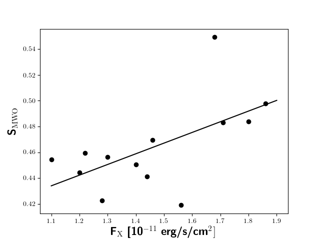
Figure 3: Correlation of most quiescent X-ray flux (set II of the X-ray fluxes, as defined in Sect. 2.3.2) and lowest S_MWO measurements within $T_{diff}=20$ days. Additionally, we show the best linear fit.

3.2 Cyclic activity behaviour

To access the cyclic activity, we employed the generalised Lomb-Scargle (GLS) periodogram (Zechmeister & Kürster 2009; Scargle 1982; Lomb 1976) as implemented in PyAstronomy (Czesla et al. 2019).

To allow a better visualisation and comparison of the data, we also applied a sinusoidal fit. We fitted the chromospheric activity indices (S_MWO, S${}_{\rm Ca\leavevmode\nobreak\ IRT}$) as a function of time with sine waves; amplitude ($A$), period ($P$), phase ($ph$), and baseline value (y-axis offset) were free parameters, and we used the period corresponding to the highest peak in the GLS as starting value for the fit. We caution that cycles may show asymmetries, as is observed on the Sun, for example, where the cycle is better described by a skewed Gaussian (Du 2011) because the rise is faster than the decay. However, Willamo et al. (2020) found that the solar cycle is particularly asymmetric compared to stellar cycles. A single chromospheric cycle of $\epsilon$ Eri shows some evidence for skewness, but a description with a sinusoidal curve nevertheless fits the data fairly well.

3.2.1 Detection of the known 3-year cycle in the X-ray data

In the previous study of the X-ray cycle by Coffaro et al. (2020), only the agreement with the short S-index cycle has been reported owing to the combination of sparse data coverage and short time baseline, and no actual search for a periodicity in the X-ray data has been performed. Using all X-ray flux measurements and their errors from the timing analysis, we are now in the position to perform a GLS analysis. This resulted in a formal detection of the 3-year cycle for the first time.

The GLS periodogram is shown in Fig. 4. We wished to avoid contribution from obvious flaring activity, but on the other hand, we did not wish to cut longer-lasting higher activity states. We therefore used X-ray flux set III as defined in Sect. 2.3.2 and determined a period of 881.33 $\pm$ 11.4 days ($\sim$ 2.4 $\pm$ 0.03 yr). To obtain the error, we simulated 10000 data sets of the X-ray flux values. Each data point was randomly drawn from a normal distribution within the standard deviation around the measured $F_{\rm X}$. The standard deviation of the obtained periods from each simulated data set was then considered as the error of the X-ray period.

Although the cycle length from the X-ray flux is somewhat shorter than previously published values from chromospheric indicators, it roughly agrees with the cycle length determined from chromospheric data taken during the approximate time-span covered by the XMM-Newton observations. This value can be found together with a more detailed discussion of the timing behaviour of the cycle length in Sect. 3.2.3.

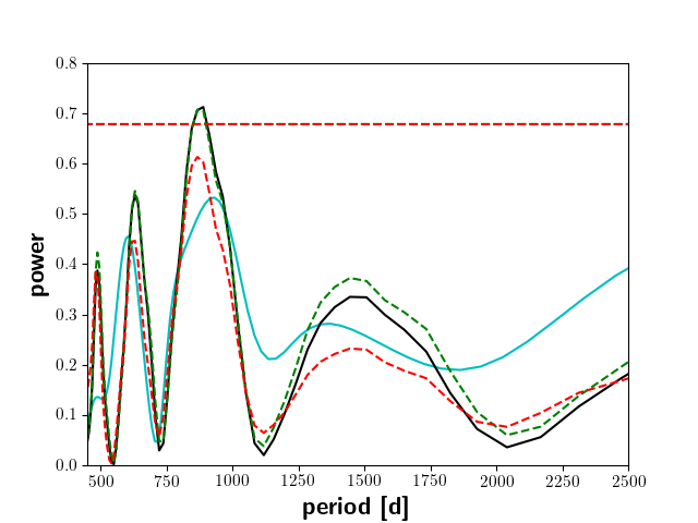
Figure 4: GLS power of the X-ray flux time series. The solid black line corresponds to the GLS power computed from the X-ray fluxes of set III defined in Sect. 2.3.2, the dashed green line corresponds to set I, and the dashed red line corresponds to set II. The solid cyan line shows the power of the GLS for the TIGRE S_MWO measurements, which are observed in about the same time interval as the X-ray data. The dashed red line shows the 1% FAP level for the X-ray GLSs.

3.2.2 Evidence for a $34$-year activity cycle from S_MWO data

The results from the GLS analysis of the S-index are shown in Fig. 6. The highest peak occurs at a rather long period of $12355\pm 230$ days ($\sim$33.8 yr) for the whole data set (the error was obtained in the same way as for the X-ray data).

This $34$-year period has also been found in the Mount Wilson program data, but was discarded by Metcalfe et al. (2013) because it was similar in length to the data set. Consistent with the result by Metcalfe et al. (2013), we also find this period in the Mount Wilson program data alone, but not in the TIGRE data alone because its time baseline is not long enough.

We show the whole time series in Fig. 5. It still covers less than two periods. Nevertheless, while the data available to Metcalfe et al. (2013) roughly extended from one maximum to the next, the more recent data show that the decay phase follows the second maximum. This adds strong evidence for a long-term periodicity. However, it is not yet clear whether this period is caused by a magnetic cycle. Jeffers et al. (2022) found a switch in the signed average magnetic field of $\epsilon$ Eri at about 2007 that approximately coincides with the maximum of our long period. This would be in line with findings for the Sun (Sanderson et al. 2003) and 61 Cygni A (Boro Saikia et al. 2016, 2018), where the reversal of the magnetic field was also found to occur around the activity maximum. Further measurements are needed to confirm whether this coincidence of magnetic field reversal and cycle maximum in $\epsilon$ Eri is caused by a magnetic cycle or occurred by chance. For the Sun, cycles longer than the Schwabe cycle (e. g. the 90-year Gleissberg cycle and the 210-year de Vries cycle) have also been discussed to be caused by noise (Cameron & Schüssler 2019). Nevertheless, the long cycle explains the observed decay of the S_MWO values between $\sim$2016-2022. To illustrate this, we performed a series of sine-curve fits on the whole S_MWO data set. All fitting parameters can be found in Table 6.

First, we fitted the data with a single sine-curve for the longest period found using its length from the GLS analysis as input parameter for the fit. This resulted in a period of $12311$ days. Fitting instead with the two known and well-established shorter cycle periods as input parameters, this leaves us with periods of $3980$ and $1061$ d. For a fit with three free periods, we obtain best-fitting periods of $12578$, $3960$, and $1062$ d. These numbers all agree with the cycle lengths obtained from the GLS analysis discussed in Sect. 3.2.3. A comparison of the standard deviations of the fits with two and with three periods ($0.035$ and $0.027$, respectively) shows that the latter period reduces the scatter in the residuals and is therefore a better description. We refrained from computing a reduced $\chi^{2}$ because no errors are assigned to the Mount Wilson data. We show the fits with one, two, and three cycles together with the S_MWO data in Fig. 5. In the bottom panel of Fig. 5, we show a zoom-in for the last nine years, also including the coronal X-ray data.

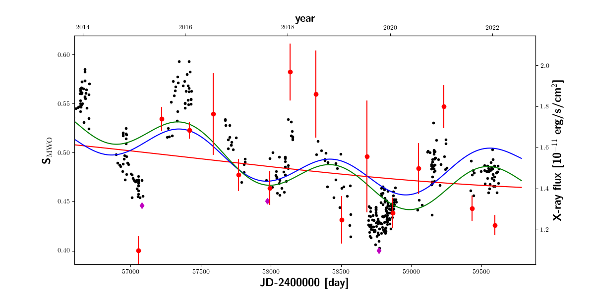
Figure 5: Time series of the S_MWO data (black dots). The best sine fit of the S_MWO data with one period is indicated by the solid red line, and the solid blue and green lines indicate the best sine fit with two and three periods, respectively. Top: All data. Bottom: Zoom into the top panel for the most recent decade. The $F_{\rm X}$ measurements from set III (red filled circles) with their errors are also plotted. In both panels, the magenta diamonds mark the data points of the minimum S_MWO value in each cycle.

3.2.3 Known 3-year and 12-year activity cycles

The periodogram also shows peaks at 3970 $\pm$ 54 days ($\sim$10.9 yr) and at 1060$\pm$30 days ($\sim$2.9 yr). These two periods have been proposed as activity cycles before, as discussed in Sect. 1, when we ascribe the longer of our periods to the 12.7 yr cycle found by Metcalfe et al. (2013). Both periods are also found when using the Mount Wilson program data or TIGRE data alone.

A high peak lies at about half of the 3 yr period; this can be identified in every data set. This peak corresponds to the alias of the 3 yr period and the one-year observation pattern. Two peaks also flank the peak at 11 yr ($\sim$3970 days), which can be identified as aliases of the 34 yr period.

We also computed a GLS in which the best-fit sine corresponded to a subtracted 34 year period, which led to a damping of these aliases, but not of the 11 yr period. Moreover, the peak of the 3 yr (=1060 days) period is then strongly enhanced. The formal false-alarm probability (FAP) for the 34-year period and the FAPs of the 11 and 3 yr period with the 34 yr period removed are all lower than $10^{-10}$. We caution, however, that the FAPs are probably underestimated because of the high number of observations.

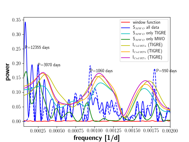
Figure 6: GLS power of the whole S_MWO time series (solid blue line) and the whole time series without the longest period (dashed blue line). We also show the GLS power of the window function (red line), of the S_MWO data of the TIGRE telescope and the Mount Wilson program data alone (cyan and green line, respectively), and of the S${}_{\rm Ca\leavevmode\nobreak\ IRT}$ of the three Ca ii IRT lines (yellow, orange, and magenta with increasing central wavelength).

Furthermore, we used fits of sine-curves for a comparison between S_MWO and S${}_{\rm Ca\leavevmode\nobreak\ IRT}$ data. We applied a fit of a single sine function representing the 3-year cycle to the TIGRE data (amplitude, period, and phase as free parameters; the initial values were set to the GLS result) and obtained a cycle length of 928 days for S_MWO data and 959, 923, and 932 days for the three S${}_{\rm Ca\leavevmode\nobreak\ IRT}$ data sets listed here in order of increasing line wavelength. The periods from the sine fits agree within 2$\sigma$ with the period value obtained from the GLS analysis of the S_MWO TIGRE data. The recovery of the $3$-year period from the GLS periodogram (see Fig. 6) in the sine-fits lends credibility to the detection of the $3$-year cycle in the S${}_{\rm Ca\leavevmode\nobreak\ IRT}$ data.

Next to the cycle length, we also compared the amplitudes of the different sine fits, $A$, but we caution that the sine fits underestimate the amplitude systematically, as can be seen in Fig. 5. We found that the sine-fit amplitude is highest for the S_MWO TIGRE data set with $A=0.034$ ($A$/offset = 7%), while the three S${}_{\rm Ca\leavevmode\nobreak\ IRT}$ data sets lead to amplitudes of $A=0.0030$ (2%), $A=0.0039$ (3%), and $A=0.0007$ (3%). This means that the reddest Ca ii IRT line is the hardest to measure because the absolute magnitude is lowest. All three Ca ii IRT lines are comparably sensitive to the cycle because the relative amplitude ($A$/offset) is about the same. However, we find a higher sensitivity of the Ca ii H&K lines to the cyclic activity variations. We list all fitting parameters of our sine fits in Table 6.

Finally, we examined the cycle length variation in the 3-year cycle, which is quite evident by the generally shorter cycle length obtained from TIGRE S_MWO data compared to the whole S_MWO data set (1061.91 days vs. 927.9 days; see Table 6). We performed a GLS search in 6-year-long time intervals and report the measured cycle length and the time intervals in Table 7. We find a minimum and maximum cycle length of 910 and 1350 days, respectively, which roughly corresponds to the relative cycle-length variations of the Sun, that is, 8–15 years (Richards et al. 2009). There is no evident pattern that would reveal a systematic variation of the cycle length.

Table 6: Best-fit parameters obtained by fitting the S_MWO and S${}_{\rm Ca\leavevmode\nobreak\ IRT}$ data with sine curves ($A\cdot\sin(2\cdot\pi/P\cdot time+ph)+$offset)

Fit	$A$	$P$	$ph$	offset
		[day]
SMWO  only 33yr period	0.03	12311.1	-63.5	0.49
SMWO  2 sine curves	0.021	3984.118	-6.273	0.49
	0.017	1061.453	1.1665
SMWO  3 sine curves	-0.0317	12578.057	60.247	0.49
	0.0187	3960.685	12.408
	-0.0191	1061.911	29.052
SMWO  TIGRE, 3yr cycle	-0.034	927.9	-1197.2	0.47
S${}_{\rm Ca\leavevmode\nobreak\ IRT}$${}_{a}^{a}$  3yr cycle	-0.0030	958.7	-662.7	0.15
S${}_{\rm Ca\leavevmode\nobreak\ IRT}$b  3yr cycle	-0.0039	922.7	-1291.3	0.12
S${}_{\rm Ca\leavevmode\nobreak\ IRT}$c  3yr cycle	-0.0007	932.4	-1117.9	0.02

Notes: ^a Indices a, b, and c refer to the individual lines of the triplet in the order of increasing wavelength.

Table 7: Length of the short (3-year) cycle in subsequent 6-year long data intervals determined from the highest GLS peak or minimum to minimum measurements.

JD first	JD last	no.	period	min-mina	ampl.b
–2400000	–2400000	spec
$[$day$]$	[day]		[day]	[day]
39786.8	41976.8	87	931.7
41977.8	44167.8	64	no peak
44168.8	46358.8	202	1128.7
46359.8	48549.8	220	no peak
48550.8	50740.8	133	1354.9
50741.8	52931.8	66	(903.3)a
52932.8	55122.8	265	1091.5	1148, 966	0.041, 0.043
55123.8	57313.8	231	1124.5	1185, 1171	0.082, 0.058
57314.8	59504.8	271	909.6	895, 796	0.044, 0.079
mean cycle length:			1063$\pm$151

Notes: ^a Does not fulfill the significance level of FAP $<$ 0.1%.

3.2.4 Length-to-amplitude law

For the Sun, a length-to-amplitude law for adjacent activity cycles is known (Hathaway 2015) that states an anti-correlation between the cycle length and the amplitude of the subsequent cycle. Hathaway et al. (1994) and Solanki et al. (2002), who studied this relation, used Sun spot number and not S-index measurements, but because these two are highly correlated, the length-to-amplitude law should hold for the S-index as well, even though the minima of these different cycle indicators are shifted slightly with respect to each other for the Sun. Moreover, the Waldmeier effect which was first known from Sun spot number as well has been shown to be present also in the solar S-index data (Garg et al. 2019).

Cycle length and amplitude can be measured for $\epsilon$ Eri for several adjacent $3$-year cycles. Fig. 5 all cycle minima of the $3$-year cycle after 2002 can be identified by eye. Before 2002, the cycle minima can only partly be identified. For some cycles, this is a result of sparser sampling, but in some cases, the cycles were less pronounced.

Analogously to the case of the solar cycle, we measured the cycle length as the time between consecutive minima (as defined by the lowest S_MWO measurements; these are highlighted in Fig. 5). We then computed the median S_MWO value of each cycle and subtracted it from the mean of the highest three S_MWO values in the respective cycle. In this way, we derived the amplitude of the cycle without relying on a single measurement (which may be affected by flaring) and also corrected for the $34$-year cycle. We used the median S_MWO value as a reference here and not the minimum because the next minimum may differ significantly, so that start and end of a cycle would not have the same activity level as measured by S_MWO. We took these measurements on the last three 6-year time intervals defined in Sect. 3.2.3, which contain two cycles each. We list the values for the cycle length and their amplitude for the six $3$-year cycles after 2002 in Table 7. Since we have length and amplitude measurements for six cycles, we have five data pairs (length of the n-th cycle and amplitude of cycle n+1) according to the length-to-amplitude law for the Sun.

We find an anti-correlation for the cycle length and the amplitude of the subsequent cycle in $\epsilon$ Eri , with a Pearson correlation coefficient of $r=-0.89$ and a probability $p=0.04$. Although the anti-correlation test is based on only five data points, it suggests comparable laws for $\epsilon$ Eri and the Sun.

3.3 Rotation period from optical measurements

The rotation period of $\epsilon$ Eri cannot be found in the whole dataset of the S_MWO data with a GLS analysis: No outstanding peak can be identified in the GLS in the range between 10 and 13 days. However, when only MWO data are used, there is an outstanding peak at about 11.1 d, but with an FAP ¿ 0.1. In the TIGRE data, the rotation period can also be identified in the S${}_{\rm Ca\leavevmode\nobreak\ IRT}$ data with an FAP lower than 3% for all three line indices and with an FAP$<$1% for the bluest line without detrending the data. The highest peak for all three Ca ii IRT lines is at a rotation period of 11.8 days, which agrees well with the periods found by Fröhlich (2007) (photometry) and Baliunas et al. (1995) (S_MWOmeasurements). The TIGRE S_MWO data instead show that the FAP of the peak at the rotation period using the S_MWO data is again much worse, but it is still the highest peak. This hiding of the rotation period can first be caused by the longer trends in the data sets (with S_MWO having a higher cycle amplitude than S${}_{\rm Ca\leavevmode\nobreak\ IRT}$), or second, by differential rotation (e.g. the period difference to the MWO data set suggests). A third possibility is the evolution of individual bright plage regions on timescales shorter than the rotation period of $\epsilon$ Eri . Again the S_MWO data would be affected more strongly because these lines are more sensitive to changes in activity than S${}_{\rm Ca\leavevmode\nobreak\ IRT}$. Strong changes in S_MWO values of $\epsilon$ Eri on timescales shorter than the rotation period have been found (Petit et al. 2021). Evolution of activity features on short timescales is also known in a different context, for instance, the evolution of prominences as found for V530 Per (Cang et al. 2020).

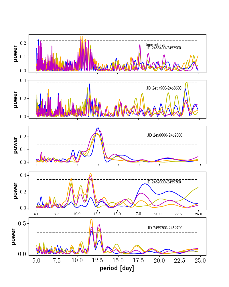
Figure 7: GLS power of the S${}_{\rm Ca\leavevmode\nobreak\ IRT}$ time series for the Ca ii IRT lines (yellow, orange, and magenta, with increasing central wavelength) and of the TIGRE S_MWO measurements (blue) for different observation seasons, see Table 8. The dashed horizontal line marks the FAP $<$0.05.

To reduce the influence of long-term variations, we computed the rotation period in five shorter time intervals that roughly corresponded to one to two TIGRE observing seasons depending on the number of observations. We list the start and end of each time span, the corresponding number of observations, and the period obtained from the highest GLS peak for each time interval and each of the four chromospheric activity indicators in Table 8. Using these shorter time spans, we subtracted a second-order polynomial from the data of each time interval and each index before computing the GLS periodogram, which we show in Fig. 7. The rotation period determined in this way shifts slightly for different observation seasons, which may be caused by differential rotation. For example we find a systematically higher rotation period of 12.3-12.5 d in all lines in the third time interval compared to all other time intervals. Petit et al. (2021) found that differential rotation on $\epsilon$ Eri ranges from about 10.8 days for equatorial spot latitudes to 13.3 days for polar latitudes. Our measurements all fall into this range, with the exception of one measurement and the few cases for which we find periods at (roughly) half, double, and $1.5$ times the rotation period for individual activity indicators and time spans (see Table 8).

A significant rotation period with an FAP $<$ 5% is found for each index in the third to fifth time intervals, except for one time interval in the S_MWO data. These time intervals roughly correspond to the late decay phase and minimum of the $34$-year activity cycle. In the first two time intervals, which correspond to the early decay phase of the $34$-year activity cycle, we do not recover the rotation period with a significant FAP, though there is a comparable number of data values available. This somewhat contra-intuitive finding may be explained by the generally high activity of $\epsilon$ Eri . It may be that during the peak of the 34-year maximum flaring or other types of activity, variations veil the variability pattern of plages rotating with the star. It is also possible that the filling factor of plages is too high to lead to a rotation pattern at activity maximum. This latter explanation is in line with the finding by Coffaro et al. (2020) regarding the corona of $\epsilon$ Eri . The corona was shown to be covered by up to $90$ % with magnetically active structures, which explains the relatively low amplitude of the X-ray cycle.

An alternative explanation may be that the first two intervals cover long times (the first interval more than one, the second interval nearly one 3-year cycle), while the latter three intervals are better sampled in time and cover each about one-third of the 3-year cycle (compare Table 8 and Fig. 5). Changes in rotation period caused by differential rotation and changing spot latitudes may therefore dilute the detection of a rotation period in the first two intervals. Interestingly, the third time interval corresponding to the 3-year cycle minimum shows the longest rotation period, while the intervals covering the rise phase and maximum of the cycle show a shorter period. This may indicate that a butterfly diagram can be found in $\epsilon$ Eri as well, with longer rotation periods (i.e. spots or plages at higher latitudes) at cycle minimum and a migration of active regions to more equatorial latitudes during the later cycle phases. Further observations with dense sampling to detect rotation periods for distinct phases of the cycle are clearly needed here.

Table 8: Rotation periods as determined from the given time intervals.

no.	min-max	period	period	period	period
spec	JD	SMWO	S${}_{\rm Ca\leavevmode\nobreak\ IRT}$a	S${}_{\rm Ca\leavevmode\nobreak\ IRT}$b	S${}_{\rm Ca\leavevmode\nobreak\ IRT}$c
	-2450000	[day]	[day]	[day]	[day]
53	6400–7900	5.2a	(11.5)	10.6	(10.5)b
39	7900–8600	(11.5)	23.5	(6.5)	(7.6)
126	8600–9000	12.5	12.2	12.3	12.5
42	9000–9300	(18.4)	11.8	11.6	11.6
41	9300–9700	11.8	11.8	11.6	12.6

Note: ^a All values have errors of 0.1 or lower computed with a Monte Carlo simulation; ^b Values in brackets have an FAP ¿ 5%.

4 Discussion and conclusions

We revisited the chromospheric and coronal activity cycle of $\epsilon$ Eri  using time series of Ca ii emission in the H&K lines and the IRT and of X-ray emission. The H&K data originate from different telescopes (including data from the Mount Wilson program, the Lowell observatory, and the TIGRE telescope) covering more than $50$ years, the Ca IRT data cover 9 years, and the X-ray flux measurements by XMM-Newton cover more than 7 years. In both chromospheric and coronal emission, we can establish the already known short ($\sim 3$ yr) activity cycle. With the analysis of the X-ray time series, we present the first quantitative detection of this cycle in X-rays, although Coffaro et al. (2020) reported X-ray fluxes from a shorter XMM-Newton data set previously, in agreement with the Ca H&K cycle. Moreover, we detected a medium-length activity cycle of about $3970$ d ($\sim$10.9 yr) in the chromospheric data, which is considerably shorter than the $12.7$ yr period found by Metcalfe et al. (2013). This discrepancy can be explained by the existence of an even longer cycle with a period of $12355$ d ($\sim$33.8 yr) that reveals its presence only in the whole data set.

Additional longer cycles, next to the well-known Schwabe (11-year) cycle, have been proposed for the Sun as well. The most prominent longer cycle is the Gleissberg ($\sim$80-100 years) cycle, which, interestingly, is roughly ten times longer than the Schwabe cycle, similar to the cycle ratio for $\epsilon$ Eri ($3$ versus $34$ yr). Several other longer and shorter periodicities have been found in proxies of solar activity, such as radioisotope concentrations (see Usoskin (2013), Hathaway (2015), and references therein). The de Vries or Suess cycle, for example, lasts $\sim$ 210 years (Suess 1980), while an even longer $\sim$2400-year cycle was discussed by Damon & Sonett (1991).

While the long $34$ yr period of $\epsilon$ Eri is highly significant in the GLS, only 1.5 cycles are covered so far, and future observations are needed to verify whether this is only a quasi-periodic episode or a true long-duration cycle. However, if it is true, this long cycle naturally explains the drop in the S_MWO data in 2018, which was interpreted as a change in the cycle behaviour by Coffaro et al. (2020).

Further properties of the solar cycle that we were able to examine on $\epsilon$ Eri based on the extraordinary long time series of chromospheric measurements are variations in cycle length. The 11-year Schwabe cycle is well known to show variations of its length that may vary roughly between 8 and 15 years for individual cycles (Richards et al. 2009). For $\epsilon$ Eri , we investigated the short cycle for length variations and found it to be variable at a standard deviation of 151 days for the measurements of the period length, with the period ranging from $910$ to $1355$ d, which is a fractional variation about as high as that of the solar $11$ yr cycle. Moreover, we tentatively also report a length-to-amplitude law in our S_MWO data as is known for the Sun from sunspot numbers. Further adjacent well-defined cycles will clarify whether the length-to-amplitude law indeed holds for $\epsilon$ Eri as well.

Our long-term monitoring of $\epsilon$ Eri also allowed us to estimate the long-term X-ray minimum state of the star by subtracting short-term variability as well as cycle variations. As representative for this long-term averaged quiescent state we considered the five XMM-Newton observations with the lowest flux in the quiescent segment of their EPIC/pn light curves (observations 1, 2, 10, 12, and 16), from which we obtain $1.21\pm 0.06\cdot 10^{-11}\,{\rm erg/cm^{2}/s}$. Comparing this to the X-ray luminosity function (XLF) of K dwarfs in Preibisch & Feigelson (2005), we found that the X-ray luminosities of only $\sim 10$ % of the field K dwarfs are higher than $\epsilon$ Eri in its lowest activity state. The activity level of $\epsilon$ Eri is high for its spectral type and is most likely to be attributed to its young age. We can therefore conclude in reversing the argument that only $\sim 10$ % of the field K dwarfs are younger than $\sim 500$ Myr, the age of $\epsilon$ Eri. When we allow that the X-ray flux of most of the stars in the XLF presented by Preibisch & Feigelson (2005) may include contributions from flares and cycles, many older stars may scatter into the upper $10$ % of the XLF, such that the fraction of young stars is likely lower than $10$ %. Improved XLFs using a Gaia-based census of the solar neighbourhood combined with updated X-ray data from the eROSITA instrument (Predehl et al. 2021), for instance, should be employed to verify this conclusion.

In summary, our multi-wavelength study provided further insight into the long-term activity of $\epsilon$ Eri : (i) We determined the coronal X-ray cycle to be $881.33$ d, in agreement with the measurement of the $3$-year cycle from the TIGRE data in the same time span as the X-ray observations. (ii) We presented strong evidence for a long 34-year activity cycle in S_MWO data. (iii) We demonstrated the detectability of the short and the medium cycle in Ca ii IRT data for the first time. The cycles give about the same values as the simultaneous S_MWO measurements, even though the amplitude of the two cycles in the Ca ii IRT data is lower. This is relevant in the context of the Gaia spectra, which cover the Ca ii IRT lines, but not the Ca ii H& K lines. Activity cycle detections should therefore be possible with Gaia RVS spectra in principle. (iv) We detected variations in cycle length of the 3-year and 11-year cycle that are comparable to that of the Sun. (v) We find a moderate correlation between X-ray flux and S-index measurements, but they are not simultaneous. This demonstrates that the long-term variation of the activity level of $\epsilon$ Eri governs the quiescent emission of chromosphere and corona. (vi) We established the long-term averaged minimum X-ray state of $\epsilon$ Eri, which places the star among the $<10$ % most active K dwarfs in the solar neighbourhood. (vii) The previously known rotation period of $11.8$ d was found in the Ca ii IRT data, but not in the S_MWO data, which indicates that these lines should (additionally) be used as indicators for rotational period and activity cycles to confirm findings by S_MWO data or when no S_MWO data are available.

Appendix A X-ray light curves

We present the light curves of the X-ray observations with short-term variability that were detected with the software R package changepoint (see Sect. 3.1) in Fig. 7. The light curves without short-term variability are shown in Fig. 8. The bottom panel in each plot shows the light curve of the hardness ratio, which was calculated from the $0.2-1.0$ keV soft band and the $1.0-2.0$ keV hard band, as defined in Eq. 1. The horizontal dash-dotted lines in each panel denote the time segments of the constant count rate that was identified with the changepoint analysis.

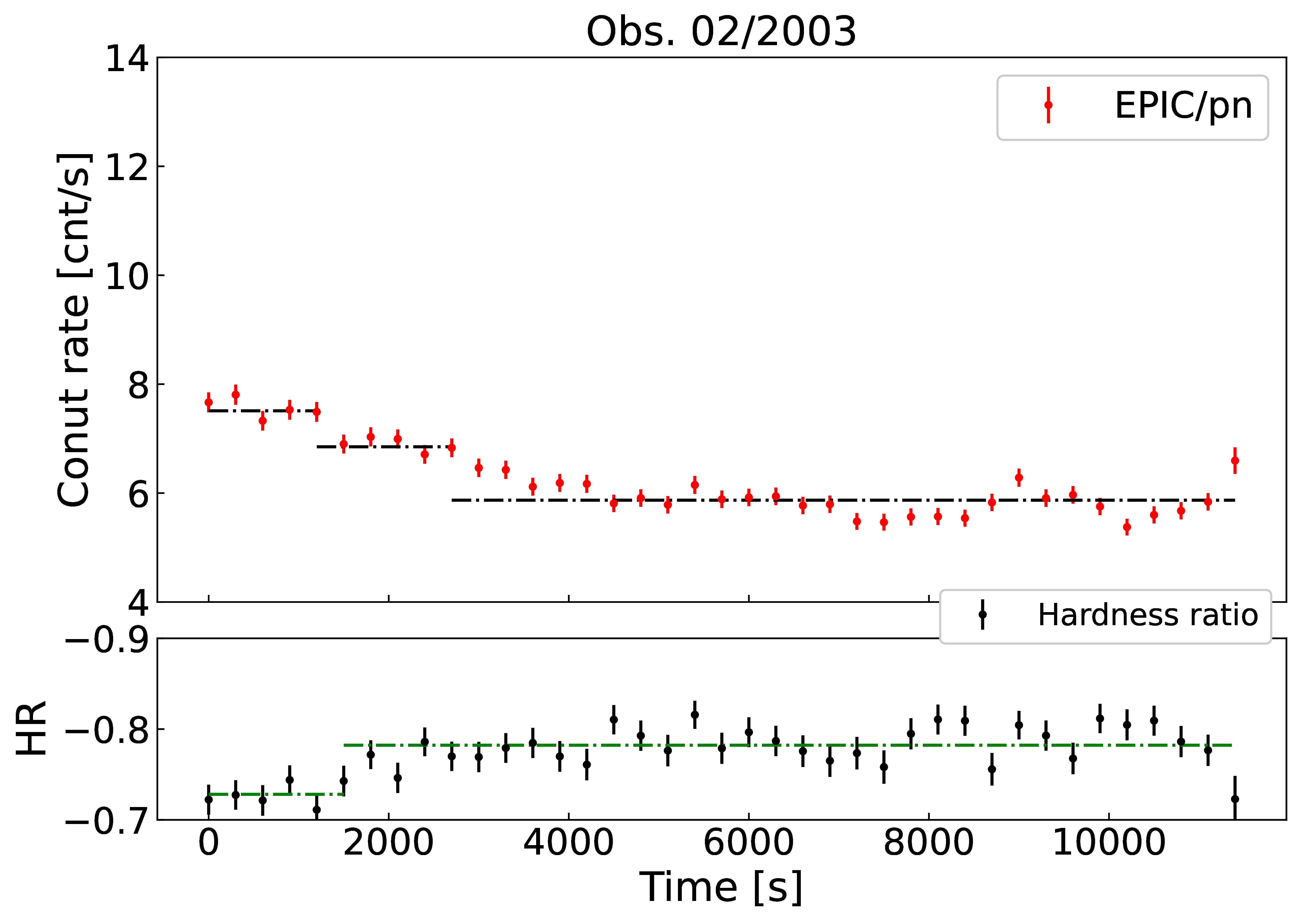
(a)

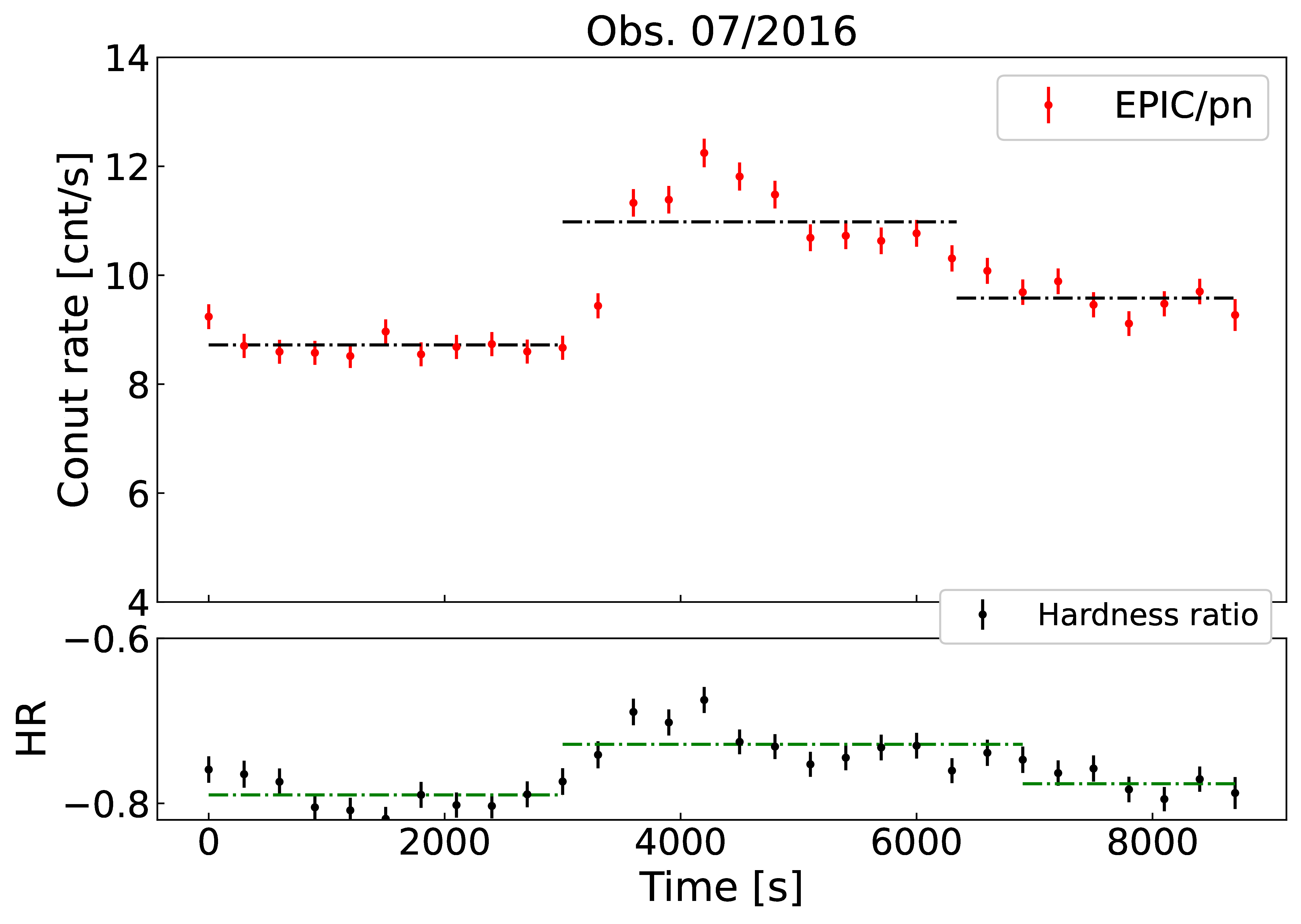
(b)

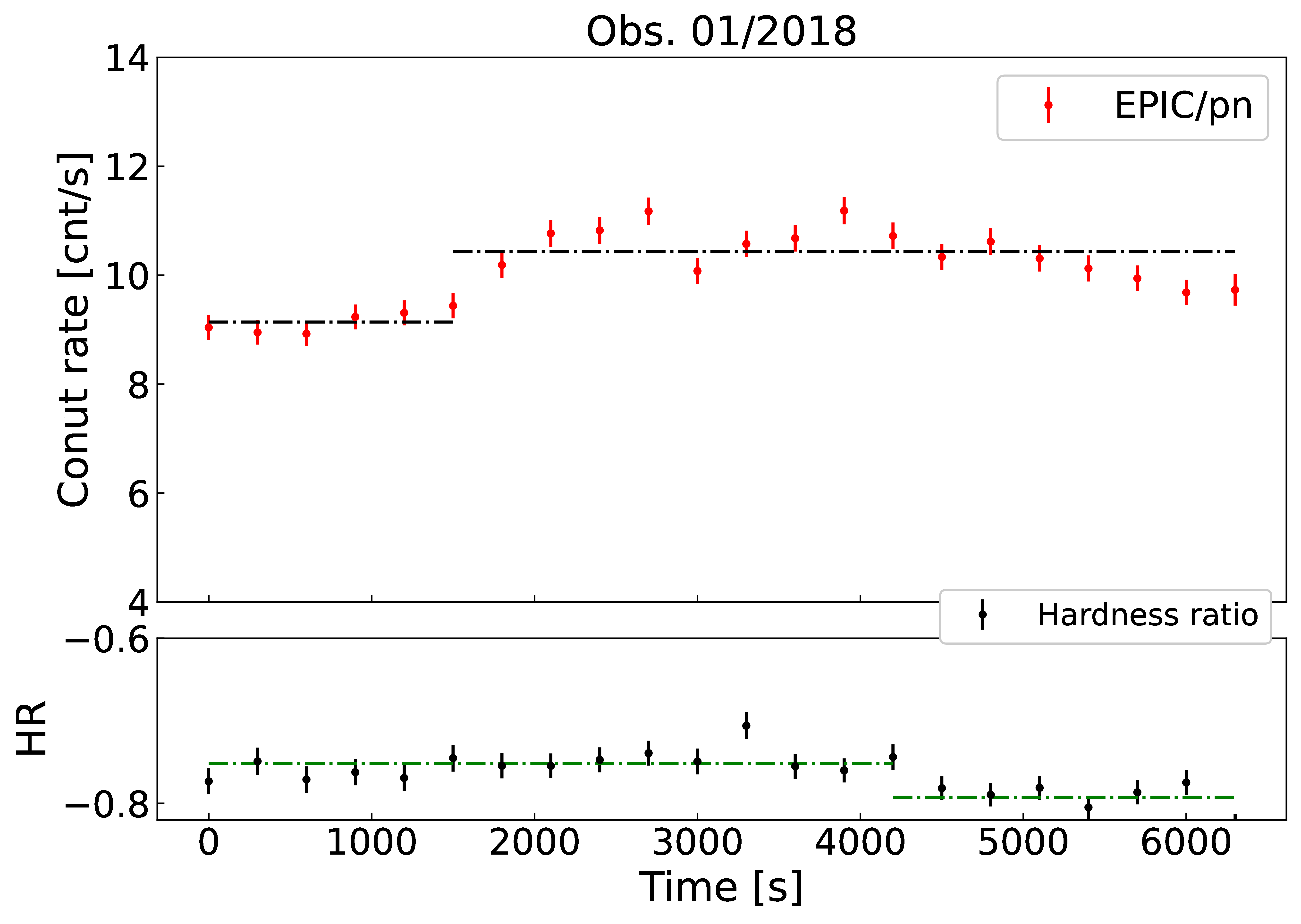
(c)

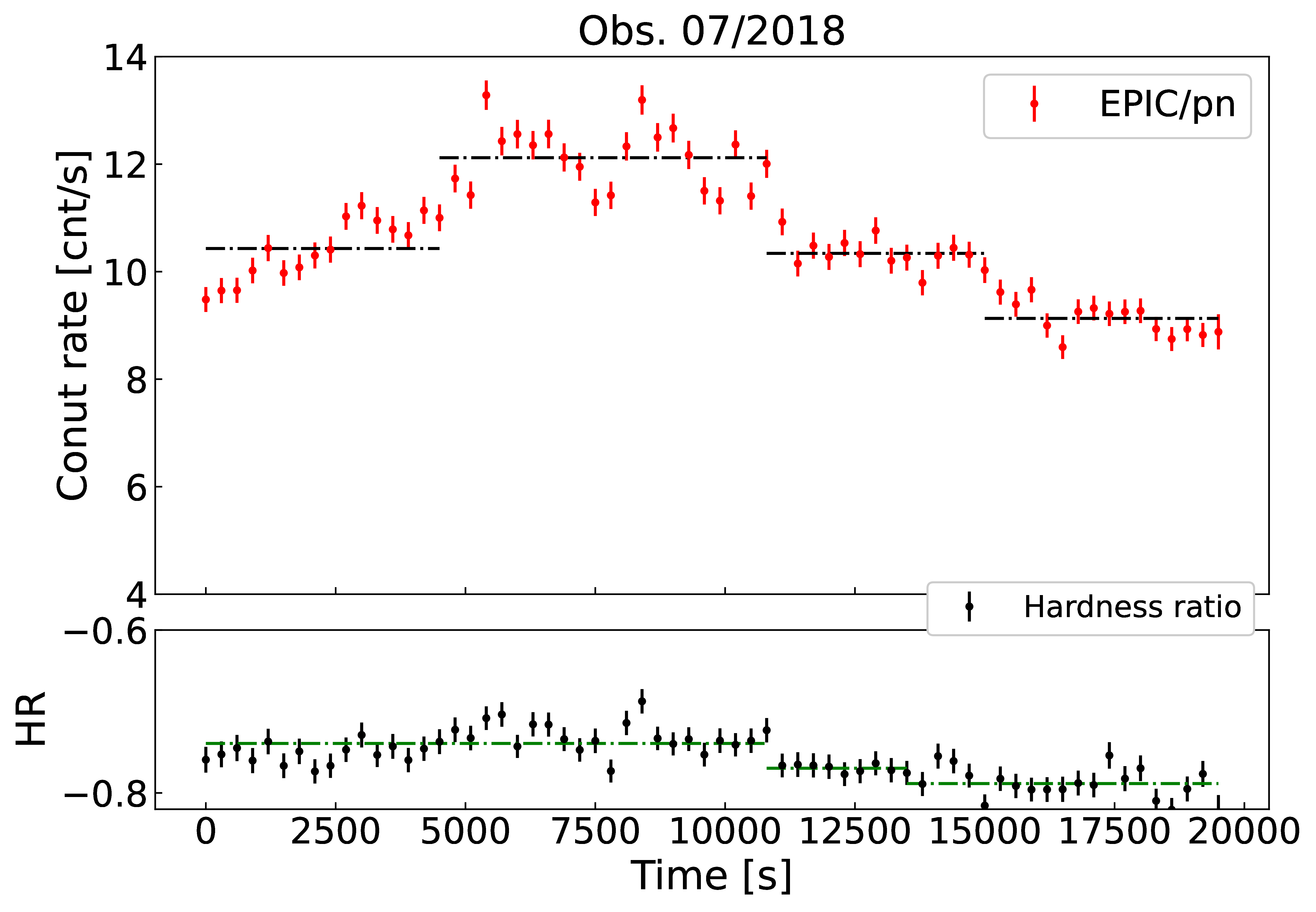
(d)

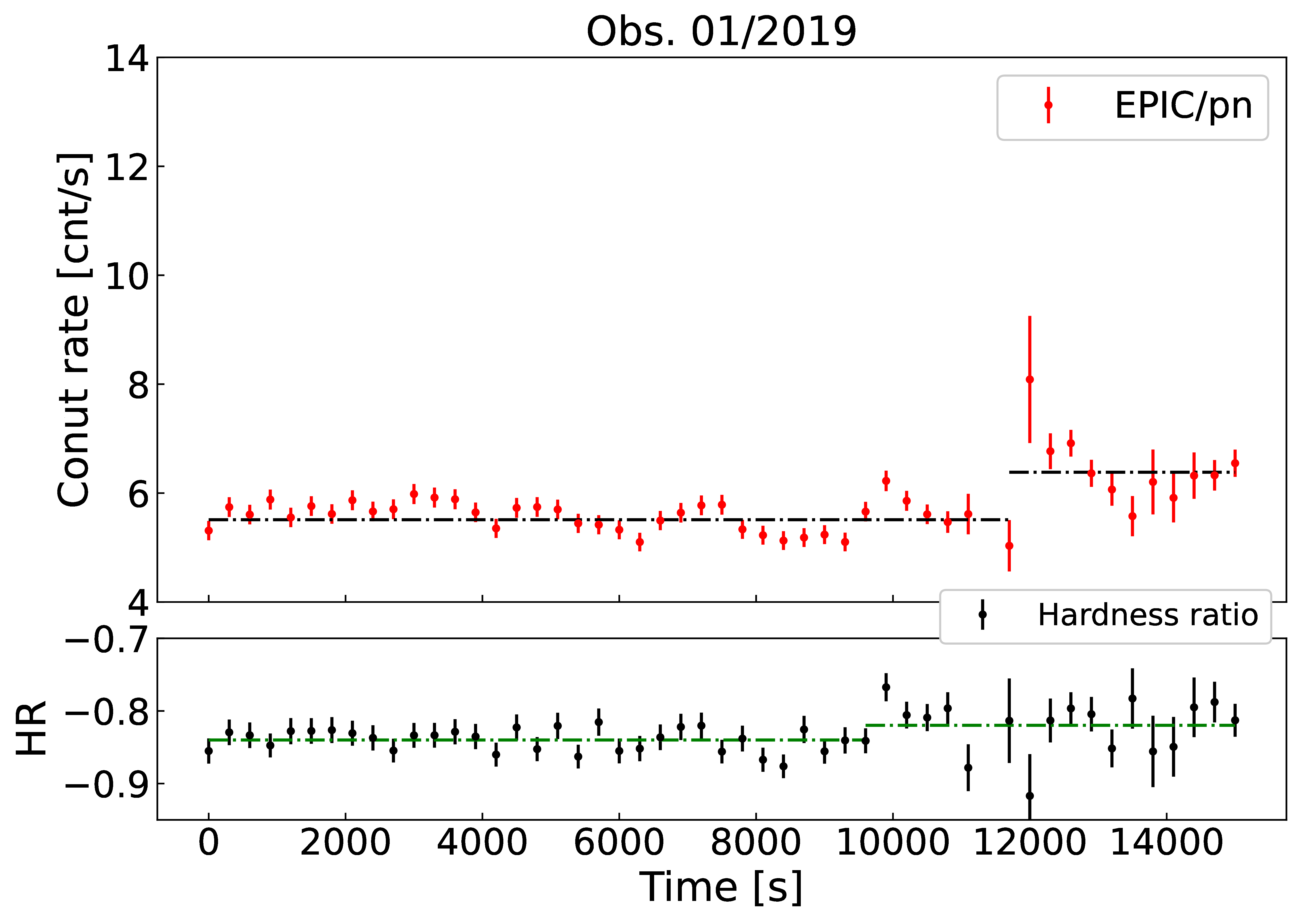
(e)

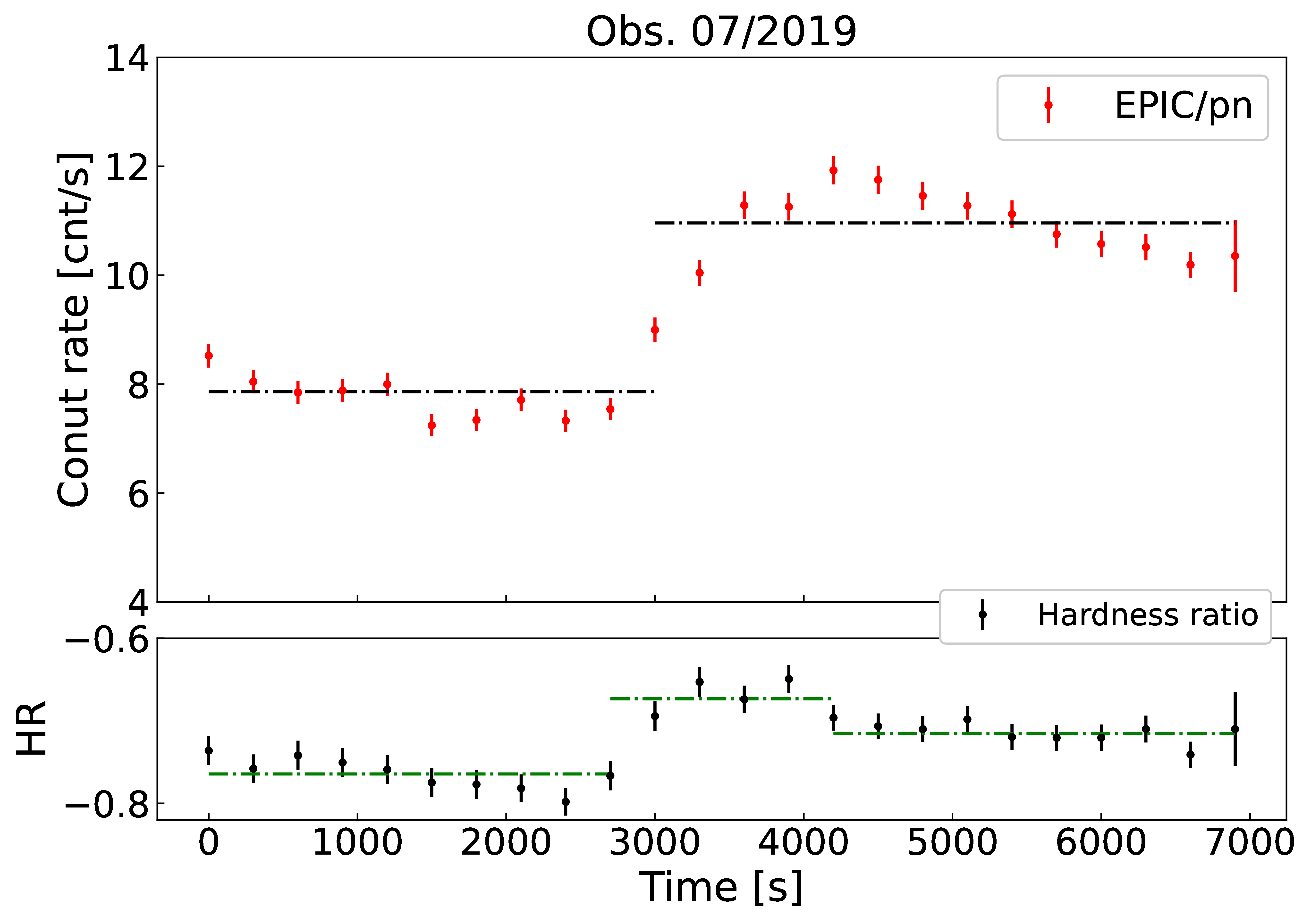
(f)

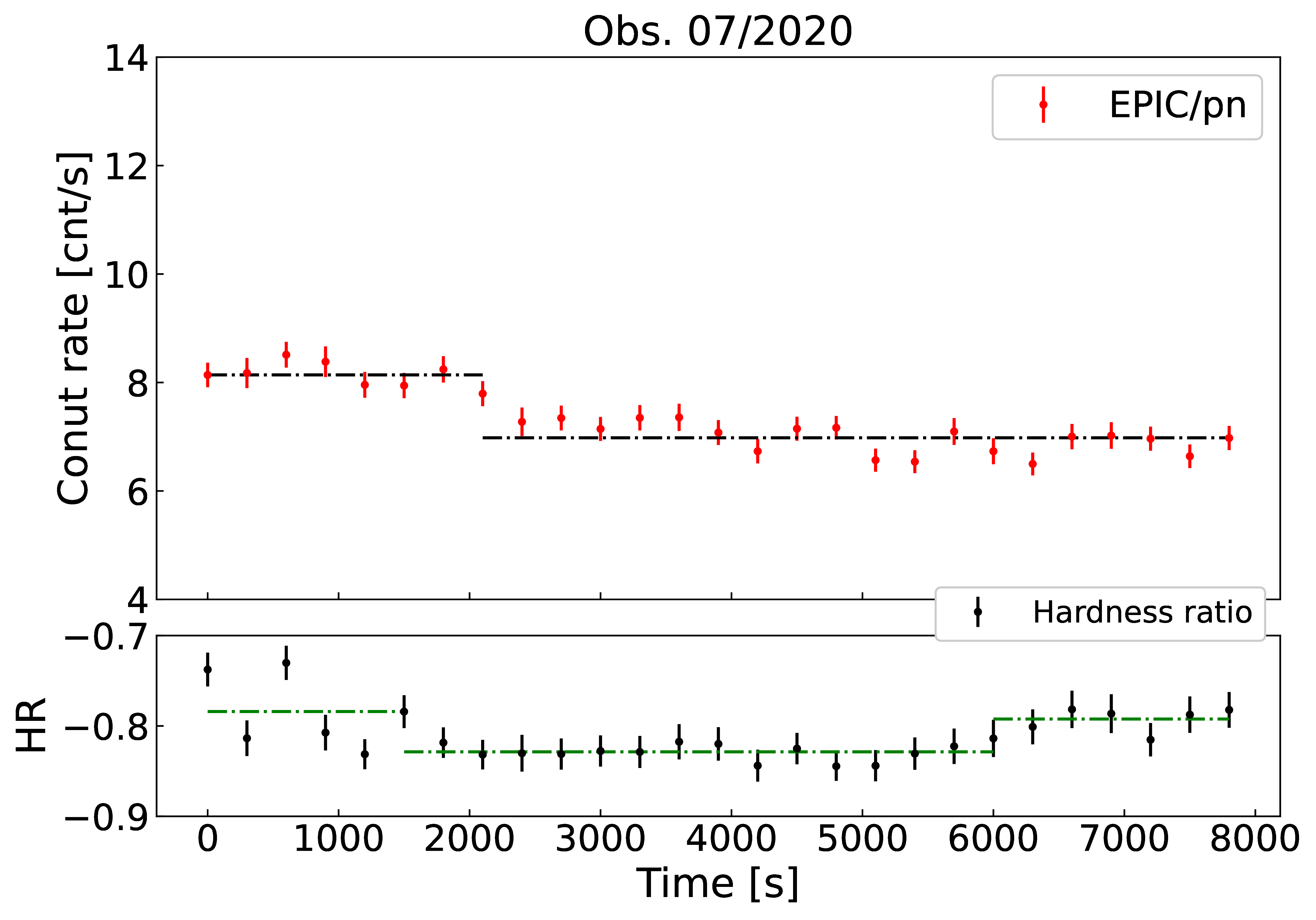
(g)

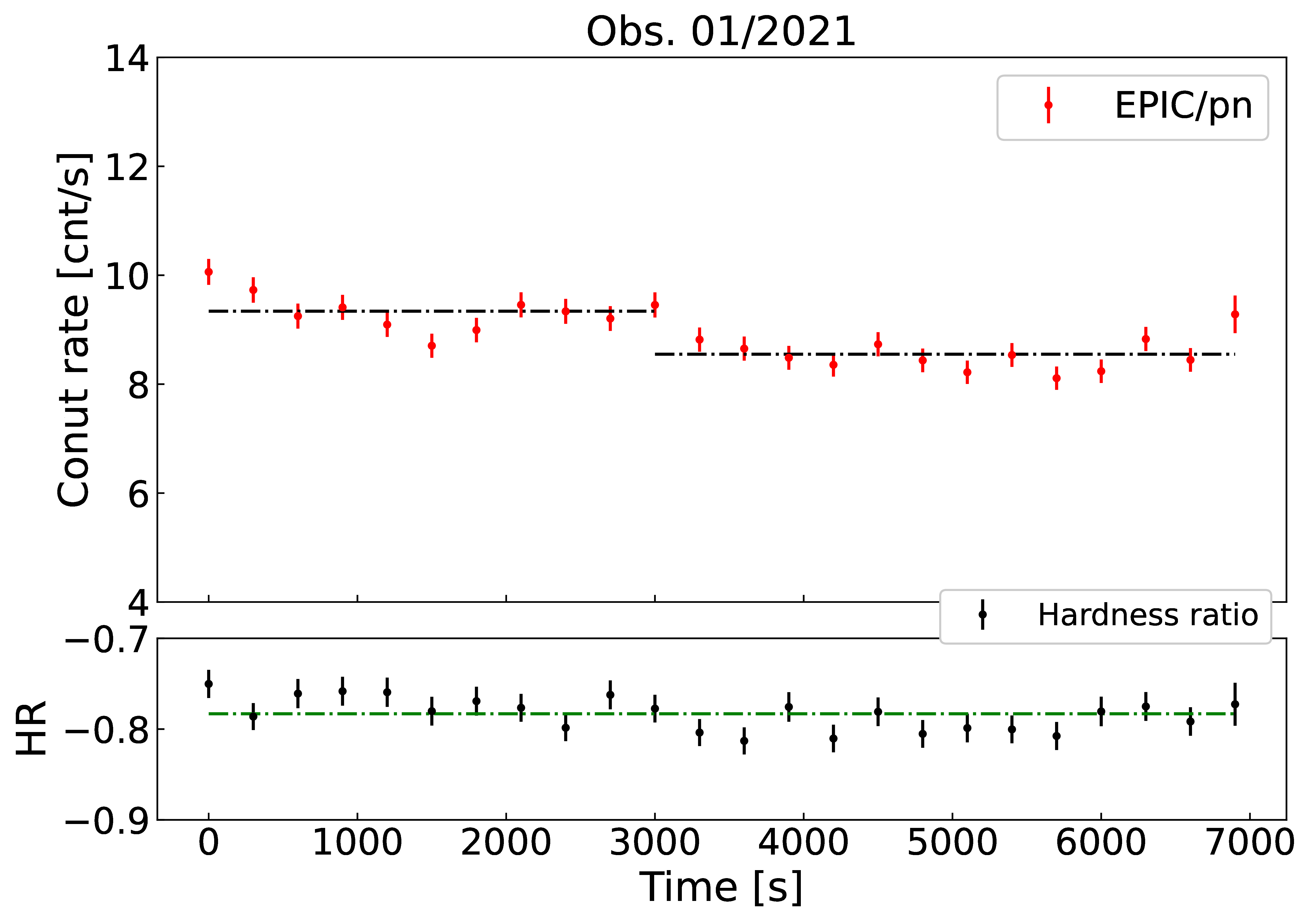
(h)

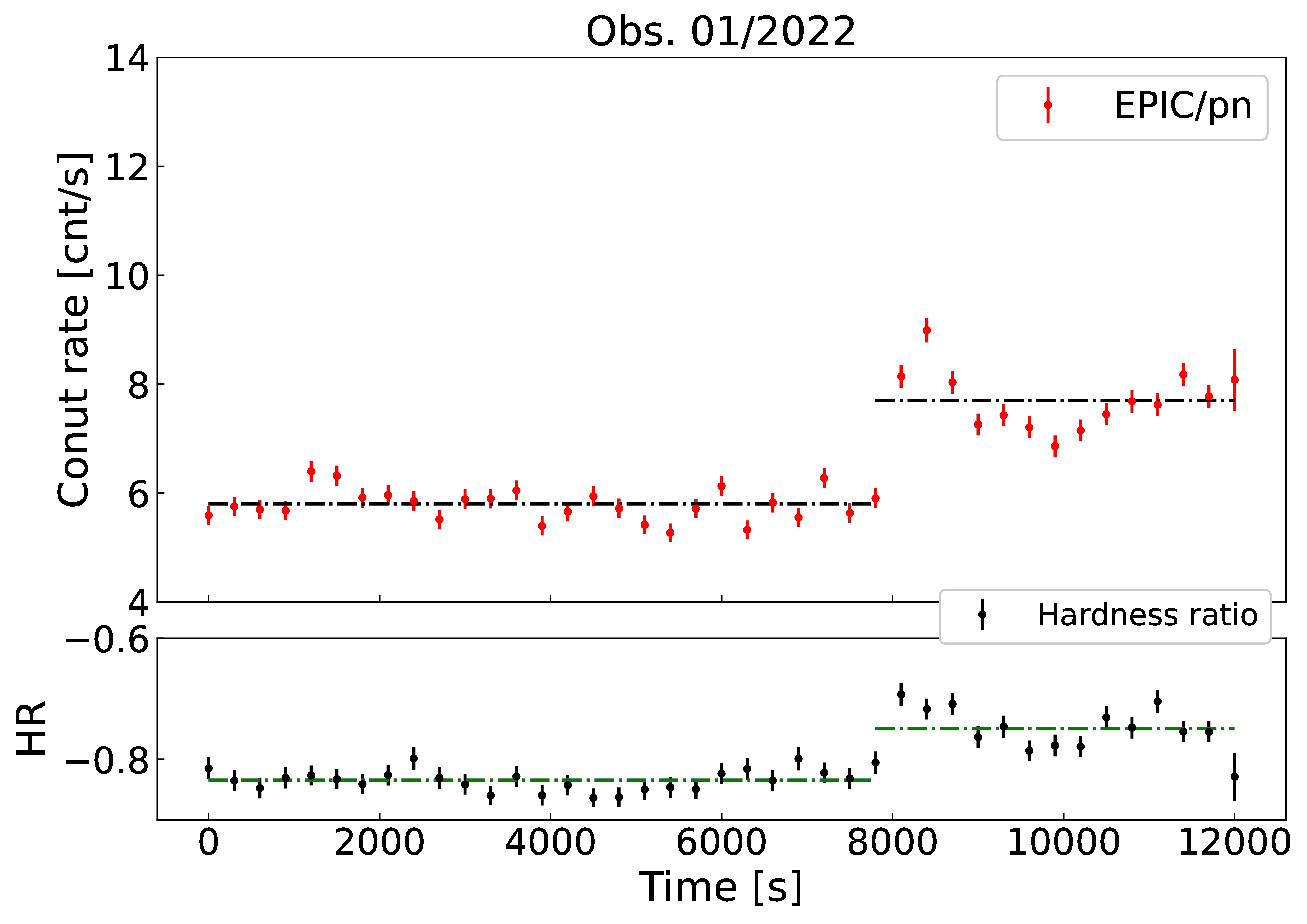
(i)

Figure 7: Light curves of $\epsilon$ Eri   extracted in the $0.2-2.0$ keV energy band and binned with a bin size of $300$ s. All observations that are flagged as variable are shown. The individual constant segments are marked with a dash-dotted horizontal black line. For each observation, the respective hardness ratio and its variation are shown in the lower panels.

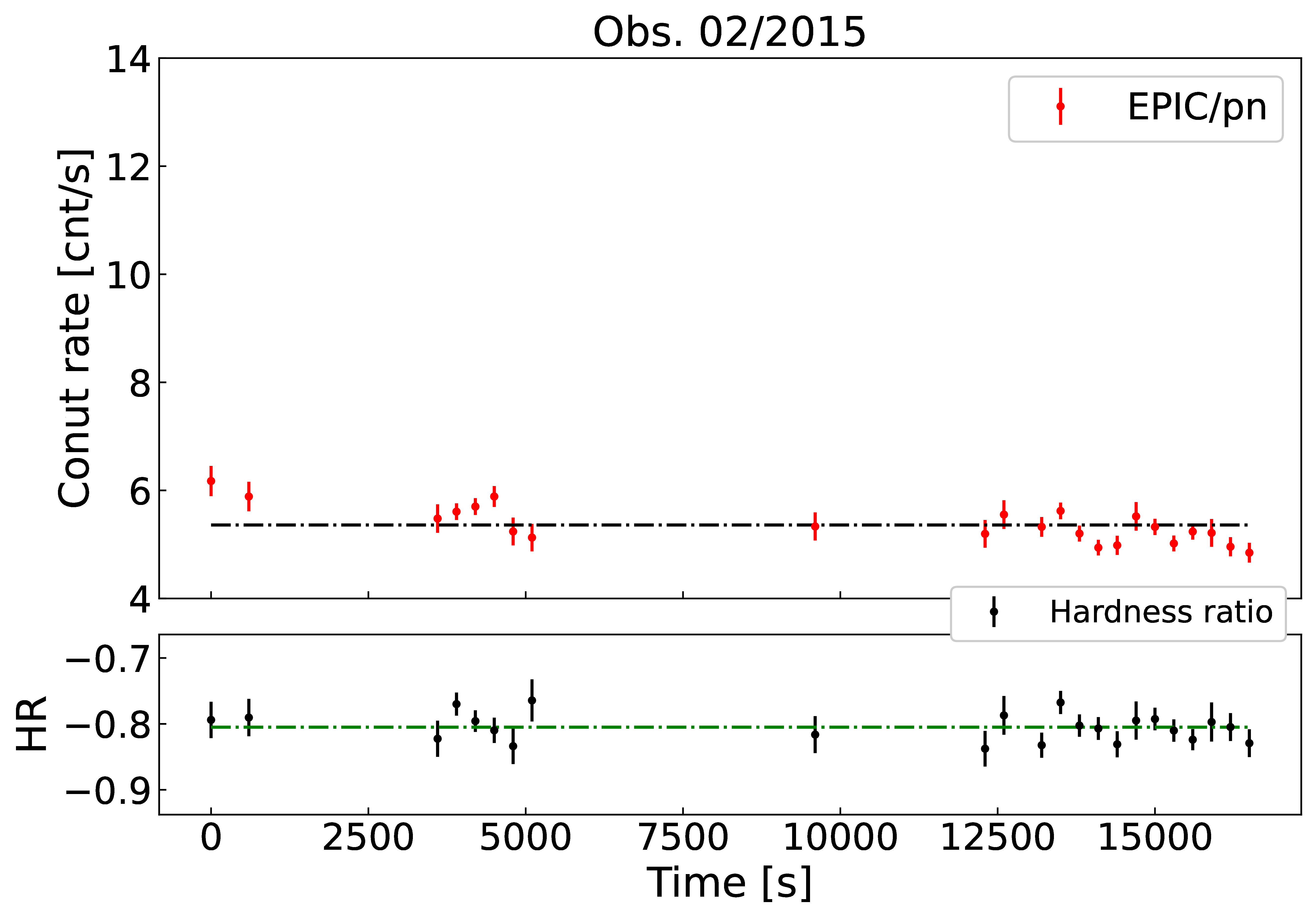
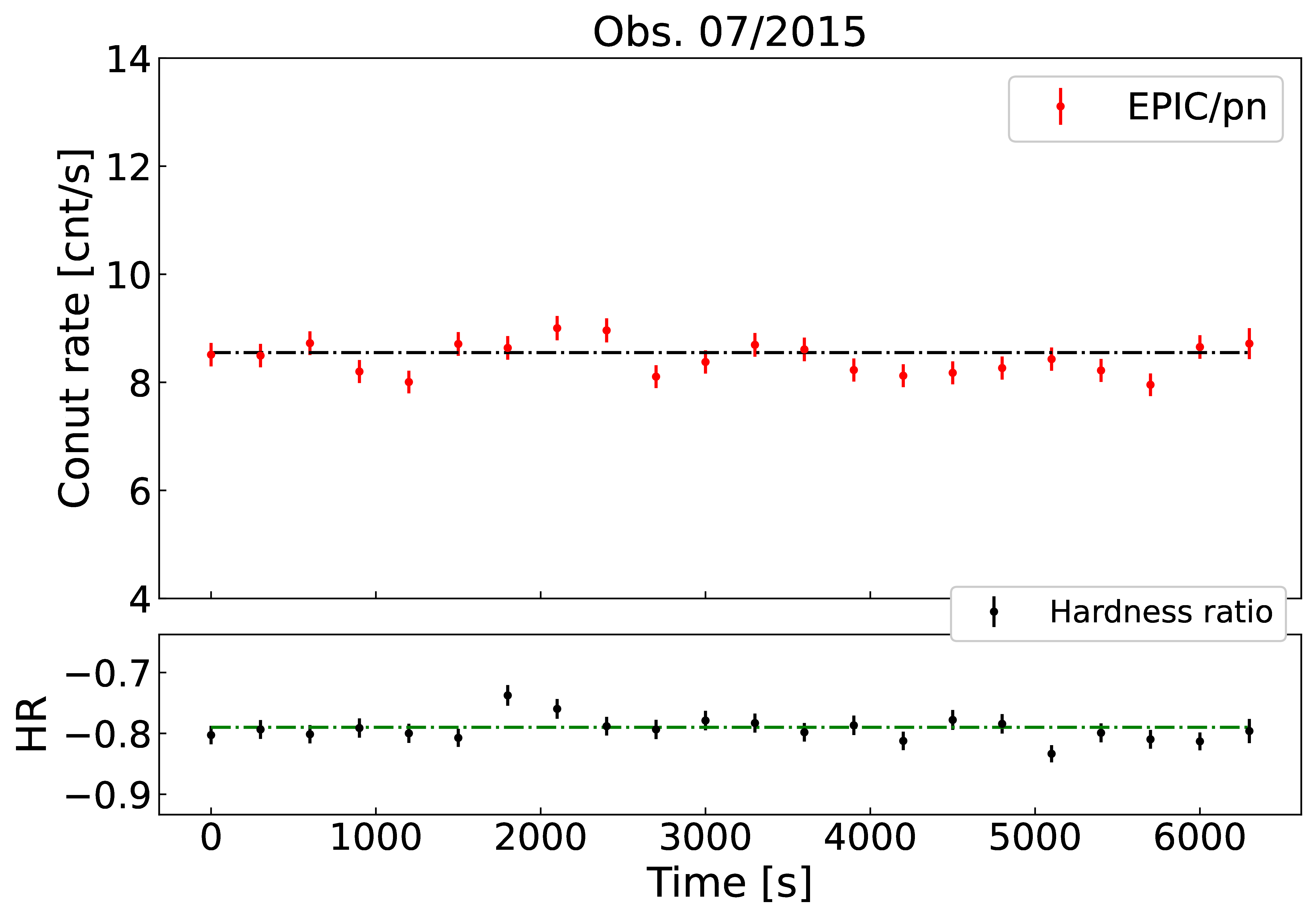
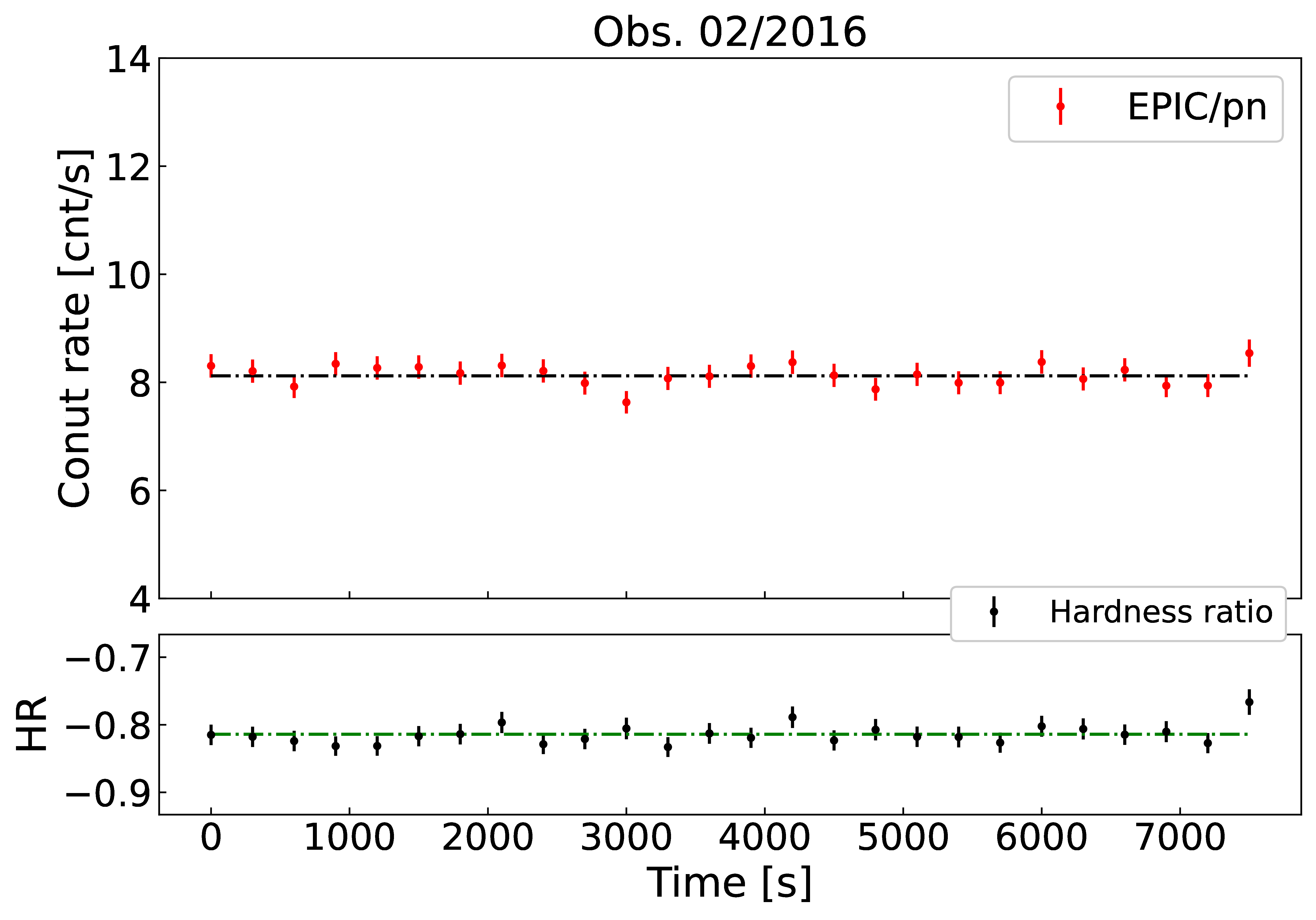
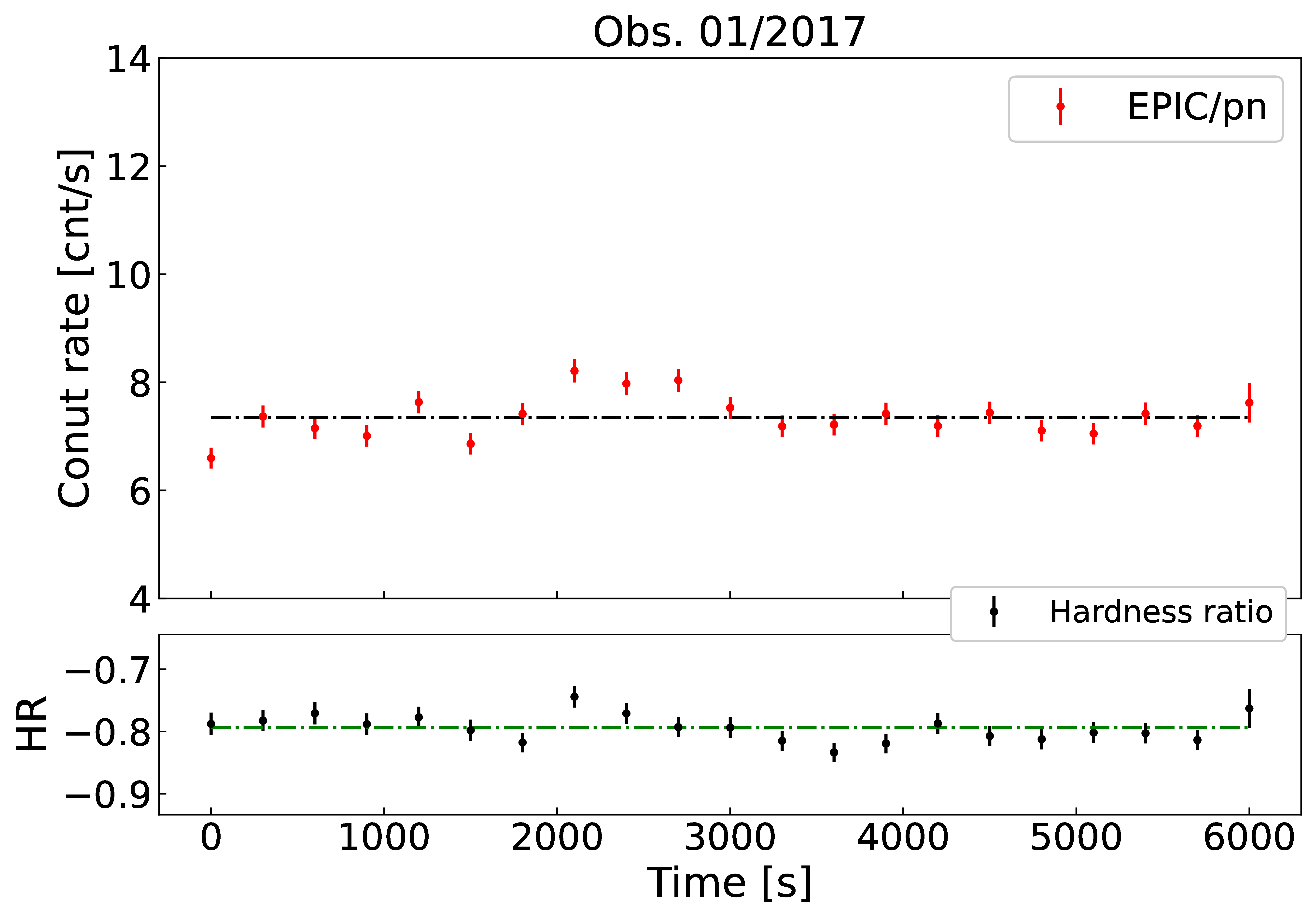
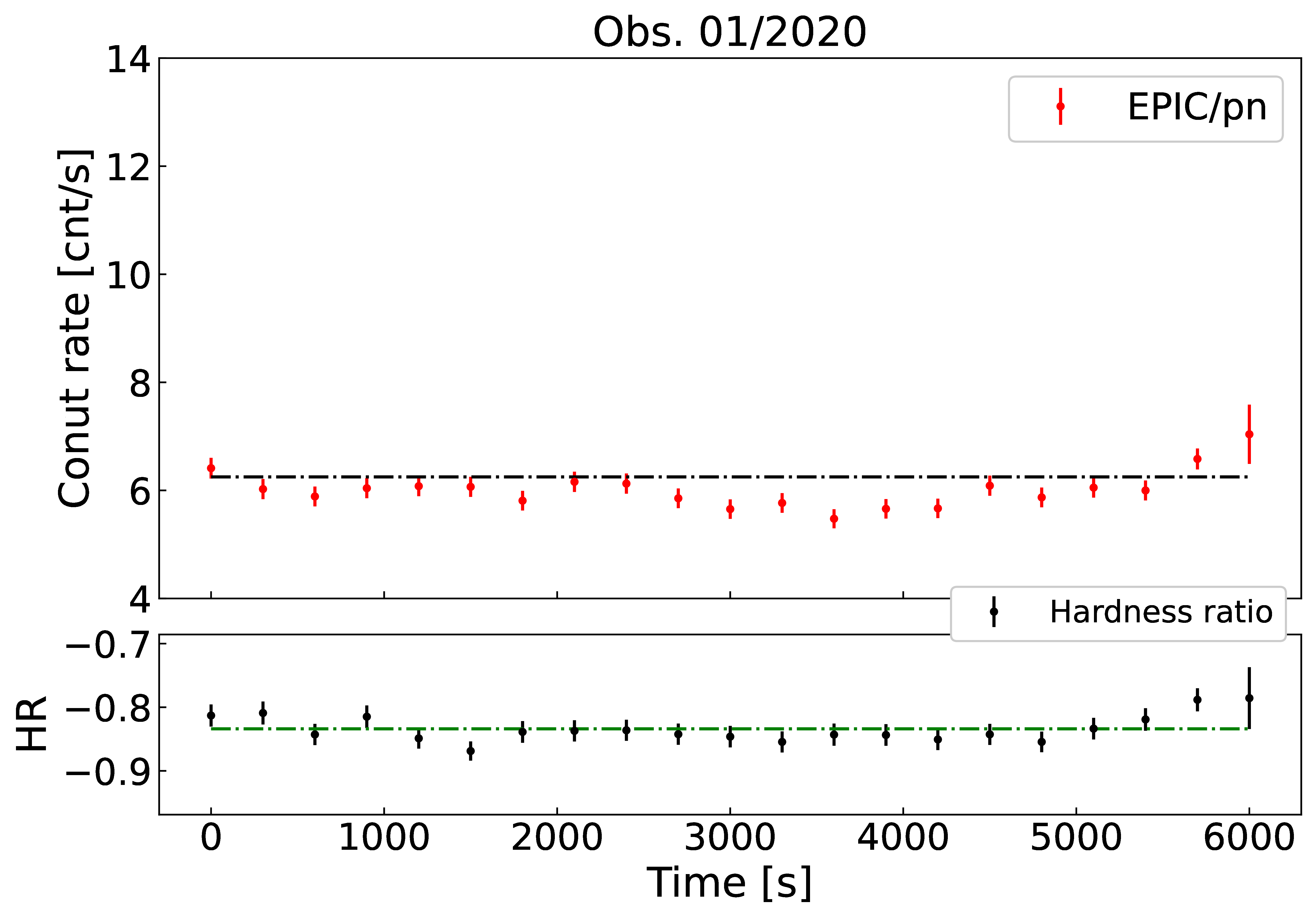
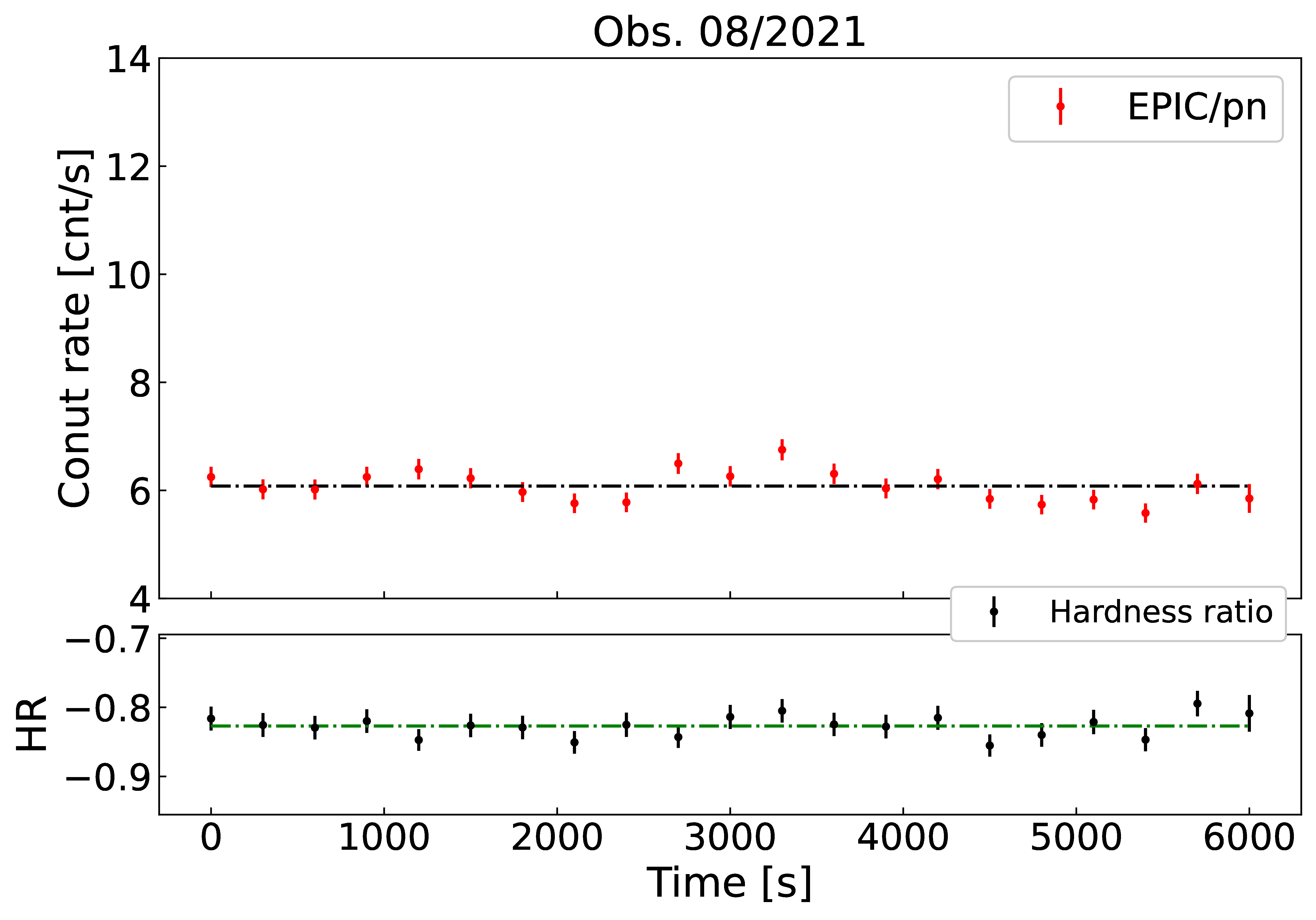
Figure 8: Same as in Fig. 7, but for the light curves without variability.