A bisection method to solve the Elvis problem with convex bounded velocity sets

Abstract.

The Elvis problem has been studied in [2], which proves existence of solutions. However, their computation in the non-smooth case remains unsolved. A bisection method is proposed to solve the Elvis problem in two space dimensions for general convex bounded velocity sets. The convergence rate is proved to be linear. Finally, numerical tests are performed on smooth and non-smooth velocity sets demonstrating the robustness of the algorithm.

1. Introduction

Suppose $\text{\boldmath${\rm{M}}$\unboldmath}_{0},\,\text{\boldmath${\rm{M}}$\unboldmath}_{1}\subseteq\mathbb{R}^{2}$ are, respectively, the lower and upper half-spaces in $\mathbb{R}^{2}$ and $\text{\boldmath$\Sigma$}={\text{\rm cl}}(\text{\boldmath${\rm{M}}$\unboldmath}_{0})\cap{\text{\rm cl}}(\text{\boldmath${\rm{M}}$\unboldmath}_{1})$ is the $x$–axis. Fix $\mathbf{x}_{0}\in\text{\boldmath${\rm{M}}$\unboldmath}_{0}$ and $\mathbf{x}_{1}\in\text{\boldmath${\rm{M}}$\unboldmath}_{1}$. Suppose speed parameters $r_{i}>0$ are also fixed associated to the domain $\text{\boldmath${\rm{M}}$\unboldmath}_{i}$ ($i=1,2$). The setting is illustrated in Figure 1.

Figure 1. The angles of incidence and Snell’s Law

The classical Snell’s Law provides a necessary condition for a trajectory to traverse from $\text{\boldmath${\rm{x}}$\unboldmath}_{0}$ to $\text{\boldmath${\rm{x}}$\unboldmath}_{1}$ in least time while using maximal speed $r_{i}$ while in $\text{\boldmath${\rm{M}}$\unboldmath}_{0}$. The condition says

$$\frac{\sin(\theta_{0})}{r_{0}}=\frac{\sin(\theta_{1})}{r_{1}},$$ (1.1)

where the $\theta_{i}$’s are the angles of incidence. However, (1.1) does not easily identify the point $\text{\boldmath${\rm{y}}$\unboldmath}\in\text{\boldmath$\Sigma$}$ through which the optimal path passes. Rather, one usually sets this up as an elementary calculus problem as minimizing $x\mapsto\frac{|\mathbf{y}-\mathbf{x}_{0}|}{r_{0}}+\frac{|\mathbf{x}_{1}-\mathbf{y}|}{r_{1}}$ over $\mathbf{y}:=\begin{pmatrix}y\\ 0\end{pmatrix}\in\text{\boldmath$\Sigma$}$.

This note provides an algorithm to find the optimal point $\mathbf{y}$ directly from (1.1) but in a much more general situation that cannot in general be reduced to elementary calculus and instead relies on Convex Analysis.

2. Analysis of the problem

We stay in $\mathbb{R}^{2}$, but similar results hold in any dimension $n$. The centered balls as the (isotropic) velocity sets above are replaced by so-called Elvis velocity sets (which could be anisotropic) whose class is denoted by ${\mathcal{C}}_{0}$. A set $\text{\boldmath${\rm{F}}$\unboldmath}\in{\mathcal{C}}_{0}$ is by definition nonempty, closed, convex, bounded, and contains ${0}$ in its interior. The least time a trajectory can go from ${0}$ to some $\text{\boldmath${\rm{v}}$\unboldmath}\in\mathbb{R}^{2}$ using velocities from ${\rm{F}}$ is recorded by the gauge function

$$\gamma_{\ \!\text{\boldmath${\rm{F}}$\unboldmath}}(\text{\boldmath${\rm{v}}$\unboldmath}):=\inf\left\{t>0:\frac{1}{t}\text{\boldmath${\rm{v}}$\unboldmath}\in\text{\boldmath${\rm{F}}$\unboldmath}\right\}=\inf\left\{t>0:\text{\boldmath${\rm{v}}$\unboldmath}\in t\text{\boldmath${\rm{F}}$\unboldmath}\right\},$$

which is a finite-valued, positively homogeneous, convex function, see [1]. The generalized Elvis problem is

$$\inf\bigl{[}\gamma_{\ \!\text{\boldmath${\rm{F}}$\unboldmath}_{0}}(\mathbf{y}-\mathbf{x}_{0})+\gamma_{\ \!\text{\boldmath${\rm{F}}$\unboldmath}_{1}}(\mathbf{x}_{1}-\mathbf{y})\bigr{]}\quad\text{over }\mathbf{y}\in\text{\boldmath$\Sigma$}. \bigl{(}P\bigr{)}$$

This is a convex optimization problem. Optimality conditions are contained in Theorem 1 which is proved in [2].

Theorem 1.

A necessary and sufficient condition for $\mathbf{y}\in\mathbb{R}^{n}$ to solve $\bigl{(}P\bigr{)}$ is the existence of $\mathbf{\zeta}_{0}$, $\text{\boldmath$\zeta$}_{1}\in\mathbb{R}^{n}$ satisfying

$$\text{\boldmath$\zeta$}_{0} \in \partial\gamma_{\,\text{\boldmath${\rm{F}}$\unboldmath}_{0}}\bigl{(}\mathbf{y}-\mathbf{x}_{0}\bigr{)},$$ (2.1)

$$-\text{\boldmath$\zeta$}_{1} \in \partial\gamma_{\,\text{\boldmath${\rm{F}}$\unboldmath}_{1}}\bigl{(}\mathbf{x}_{1}-\mathbf{y}\bigr{)},\quad\text{and}$$ (2.2)

$$\text{\boldmath$\zeta$}_{0}+\text{\boldmath$\zeta$}_{1} \in -\text{\boldmath${\rm{N}}$\unboldmath}_{\text{\boldmath$\Sigma$}}(\mathbf{y}).$$ (2.3)

where $\text{\boldmath${\rm{N}}$\unboldmath}_{\text{\boldmath$\Sigma$}}(\mathbf{y})$ is the normal cone of $\Sigma$ at $\mathbf{y}$, which in this case is always the $y$-axis.

Remark 2.1.

Note that solutions $\mathbf{y}\in\mathbb{R}^{n}$ may not be unique if the velocity sets $F_{0}$ and $F_{1}$ are not strictly convex.

We call (2.3) the generalized Snell’s Law from which the classical version (1.1) can be derived as follows. Let us note the polar of $\text{\boldmath${\rm{F}}$\unboldmath}\in{\mathcal{C}}_{0}$ as $\text{\boldmath${\rm{F}}$\unboldmath}^{\circ}$, which is defined by $\text{\boldmath${\rm{F}}$\unboldmath}^{\circ}:=\{\mathbf{\zeta}\in\mathbb{R}^{n}:\;\forall\mathbf{v}\in\text{\boldmath${\rm{F}}$\unboldmath},\langle\text{\boldmath$\zeta$},\mathbf{v}\rangle\leq 1\}$; it also belongs to ${\mathcal{C}}_{0}$. It is shown in [2] that (2.1) and (2.2) imply that the optimal velocities are

$$\mathbf{v}_{0}:=\frac{\mathbf{y}-\mathbf{x}_{0}}{\gamma_{\,\text{\boldmath${\rm{F}}$\unboldmath}_{0}}(\mathbf{y}-\mathbf{x}_{0})}\in\text{\boldmath${\rm{F}}$\unboldmath}_{0},\quad\mathbf{v}_{1}:=\frac{\mathbf{x}_{1}-\mathbf{y}}{\gamma_{\,\text{\boldmath${\rm{F}}$\unboldmath}_{1}}(\mathbf{x}_{1}-\mathbf{y})}\in\text{\boldmath${\rm{F}}$\unboldmath}_{1},$$

and that

$$\text{\boldmath$\zeta$}_{0}\in\text{\boldmath${\rm{N}}$\unboldmath}_{\,\text{\boldmath${\rm{F}}$\unboldmath}_{0}}\left(\mathbf{v}_{0}\right),\;-\text{\boldmath$\zeta$}_{1}\in\text{\boldmath${\rm{N}}$\unboldmath}_{\,\text{\boldmath${\rm{F}}$\unboldmath}_{1}}\left(\mathbf{v}_{1}\right),\;\text{and }\gamma_{\,\text{\boldmath${\rm{F}}$\unboldmath}^{\circ}_{0}}(\text{\boldmath$\zeta$}_{0})=1=\gamma_{\,\text{\boldmath${\rm{F}}$\unboldmath}^{\circ}_{1}}(-\text{\boldmath$\zeta$}_{1}).$$ (2.4)

If $\text{\boldmath${\rm{F}}$\unboldmath}_{0}=r_{0}\text{\boldmath$\overline{\rm{B}}$\unboldmath}$ and $\text{\boldmath${\rm{F}}$\unboldmath}_{1}=r_{1}\text{\boldmath$\overline{\rm{B}}$\unboldmath}$, then $\text{\boldmath${\rm{F}}$\unboldmath}^{\circ}_{0}=\frac{1}{r_{0}}\text{\boldmath$\overline{\rm{B}}$\unboldmath}$ and $\text{\boldmath${\rm{F}}$\unboldmath}^{\circ}_{1}=\frac{1}{r_{1}}\text{\boldmath$\overline{\rm{B}}$\unboldmath}$. The last statement in (2.4) then says

$$\text{\boldmath$\zeta$}_{0}=\frac{1}{r_{0}}\begin{pmatrix}\sin(\theta_{0})\\ \cos(\theta_{0})\end{pmatrix}\quad\text{and}\quad-\text{\boldmath$\zeta$}_{1}=\frac{1}{r_{1}}\begin{pmatrix}\sin(\theta_{1})\\ \cos(\theta_{1})\end{pmatrix}$$

for some angles $\theta_{0}$, $\theta_{1}$. The condition (2.3) says the $x$-component $\text{\boldmath$\zeta$}_{0}+\text{\boldmath$\zeta$}_{1}$ is $0$, which is (1.1). The first condition in (2.4) implies $\text{\boldmath${\rm{u}}$\unboldmath}\mapsto\langle\text{\boldmath$\zeta$}_{0},\text{\boldmath${\rm{u}}$\unboldmath}\rangle$ is maximized over $\text{\boldmath${\rm{u}}$\unboldmath}\in\text{\boldmath${\rm{F}}$\unboldmath}_{0}$ at $\mathbf{v}_{0}$ and the second condition in (2.4) implies $\text{\boldmath${\rm{u}}$\unboldmath}\mapsto\langle-\text{\boldmath$\zeta$}_{1},\text{\boldmath${\rm{u}}$\unboldmath}\rangle$ is maximized over $\text{\boldmath${\rm{u}}$\unboldmath}\in\text{\boldmath${\rm{F}}$\unboldmath}_{1}$ at $\mathbf{v}_{1}$. The angles have therefore the same geometric meaning as in Figure 1. However, the optimal $\mathbf{y}$ remains unknown.

3. Bisection method

We provide an algorithm to approximate solutions of $\bigl{(}P\bigr{)}$. For $\text{\boldmath${\rm{z}}$\unboldmath}=\begin{pmatrix}x\\ y\end{pmatrix}\in\mathbb{R}^{2}$, let $\Pi_{\Sigma}(\text{\boldmath${\rm{z}}$\unboldmath})=x$ be the $x$-component of the orthogonal projection onto $\Sigma$. It is assumed thereafter that $\Pi_{\Sigma}(\mathbf{x}_{0})<\Pi_{\Sigma}(\mathbf{x}_{1})$. The goal of the algorithm is to compute the optimal $\mathbf{y}=\begin{pmatrix}y\\ 0\end{pmatrix}$ that solves $\bigl{(}P\bigr{)}$. As the problem is not very regular, the existence of second order gradients is not assured. Therefore, the gradient-free bisection method is chosen.

3.1. The algorithm

Let $\varepsilon>0$ be a tolerance parameter. Algorithm 1 is used to approximate a solution of $\bigl{(}P\bigr{)}$.

1. Set $l^{0}:=\Pi_{\text{\boldmath$\Sigma$}}(\mathbf{x}_{0})$, $r^{0}:=\Pi_{\text{\boldmath$\Sigma$}}(\mathbf{x}_{1})$ and $y^{0}:=\frac{1}{2}\left(l^{0}+r^{0}\right)$

2. For $k\in\mathbb{N}^{*}$, let $\mathbf{y}^{k}=\begin{pmatrix}y^{k}\\ 0\end{pmatrix}$ and

   $$\mathbf{v}_{0}^{k}:=\mathbf{y}^{k}-\mathbf{x}_{0}\quad \text{and}\quad\gamma_{0}^{k}:=\gamma_{\,\text{\boldmath${\rm{F}}$\unboldmath}_{0}}\left(\mathbf{v}_{0}^{k}\right)$$

   $$\mathbf{v}_{1}^{k}:=\mathbf{x}_{1}-\mathbf{y}^{k}\quad \text{and}\quad\gamma_{1}^{k}:=\gamma_{\,\text{\boldmath${\rm{F}}$\unboldmath}_{1}}\left(\mathbf{v}_{1}^{k}\right).$$

3. Calculate (or choose any) $\text{\boldmath$\zeta$}_{0}^{k}$, $\text{\boldmath$\zeta$}_{1}^{k}$ so that

   $$\text{\boldmath$\zeta$}_{0}^{k}\in\;\text{\boldmath${\rm{N}}$\unboldmath}_{\text{\boldmath${\rm{F}}$\unboldmath}_{0}}\left({\mathbf{v}_{0}^{k}}/{\gamma_{0}^{k}}\right)\quad \text{with}\quad\gamma_{\,\text{\boldmath${\rm{F}}$\unboldmath}_{0}^{\circ}}(\text{\boldmath$\zeta$}_{0}^{k})=1$$

   $$-\text{\boldmath$\zeta$}_{1}^{k}\in\;\text{\boldmath${\rm{N}}$\unboldmath}_{\text{\boldmath${\rm{F}}$\unboldmath}_{1}}\left({\mathbf{v}_{1}^{k}}/{\gamma_{1}^{k}}\right)\quad \text{with}\quad\gamma_{\,\text{\boldmath${\rm{F}}$\unboldmath}_{1}^{\circ}}(-\text{\boldmath$\zeta$}_{1}^{k})=1$$

4. Set $\delta=\Pi_{\text{\boldmath$\Sigma$}}(\text{\boldmath$\zeta$}_{0}+\text{\boldmath$\zeta$}_{1})$.

   1. If $|\delta|\leq\varepsilon$, then the process terminates and $\mathbf{y}^{k}$ is the solution.

   2. If $\delta<-\varepsilon$, then set $l^{k+1}:=l^{k}$, $y^{k+1}:=\frac{1}{2}\left(r^{k}+y^{k}\right)$ and $r^{k+1}:=y^{k}$, and start over at step 2.

   3. If $\delta>\varepsilon$, then set $r^{k+1}:=r^{k}$, $y^{k+1}:=\frac{1}{2}\left(l^{k}+y^{k}\right)$ and $l^{k+1}:=y^{k}$, and start over at step 2.

Algorithm 1 Bisection

Remark 3.1.

Note that if $\Pi_{\Sigma}(\mathbf{x}_{0})>\Pi_{\Sigma}(\mathbf{x}_{1})$, then the test $(b)$ and $(c)$ in step $(4)$ of the algorithm are reversed.

3.2. Convergence proof

Let $d^{k}:=r^{k}-l^{k}>0$. Thus, $d^{0}=\Pi_{\text{\boldmath$\Sigma$}}(\mathbf{x}_{1})-\Pi_{\text{\boldmath$\Sigma$}}(\mathbf{x}_{0})$. By construction, one has $d^{k+1}=\frac{d^{k}}{2}$. Therefore,

$$\bigl{|}\mathbf{y}^{k}-\mathbf{y}\bigr{|}\leq d^{k}=\frac{d^{0}}{2^{k}}$$

Thus, $\mathbf{y}^{k}\to\mathbf{y}$ when $k\to\infty$ with a linear convergence rate.

4. Numerical results

We first verify that the convergence rate is linear and then provide an example with non-strictly convex and non-smooth velocity sets.

4.1. Elliptic velocity sets

We take $\varepsilon$ to be the machine error. The test case consists in having $\mathbf{x}_{0}:=(-1,-1)$ and $\mathbf{x}_{1}:=(1,1)$. The velocity sets are the following ellipses $\text{\boldmath${\rm{F}}$\unboldmath}_{0}:=(\cos(t),\sin(t)/2)$ and $\text{\boldmath${\rm{F}}$\unboldmath}_{1}:=(2\cos(t),\sin(t))$, for $t\in[0,2\pi]$.

The green curve in Figure 2 represents $\Pi_{\Sigma}(\text{\boldmath${\rm{N}}$\unboldmath}_{\text{\boldmath${\rm{F}}$\unboldmath}_{0}}-\text{\boldmath${\rm{N}}$\unboldmath}_{\text{\boldmath${\rm{F}}$\unboldmath}_{1}})$. The reference solution is computed as the abscissa of the unique point of the green curve in Figure 2 which has a zero ordinate.

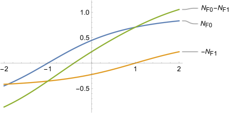
Figure 2. Ellipitc velocity sets: Reference solution.

The reference solution is thus computed as

$$y^{\text{ref}}:=-0.401.$$

The algorithm finds the result up to $\varepsilon$ as shown in the convergence plot of the error is given in Figure 3.

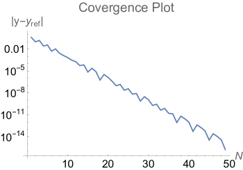
Figure 3. Ellipcitc velocity sets: Convergence plot.

A linear regression gives a variance estimated at $5.2\cdot 10^{-3}$ for a line of equation $\log(|y^{k}-y^{\text{ref}}|)=-0.88-0.0011k$ thus confirming the linear convergence of the algorithm.

4.2. Polyhedral velocity sets

We take $\varepsilon$ to be the machine error. The test case consists in having $\mathbf{x}_{0}:=(0,-1)$ and $\mathbf{x}_{1}$ considered in several regions. The velocity sets are the squares plotted in Figure 4, both containing the origin.These velocity sets were constructed to give rise to three regions of solutions, as can be seen in the raycast propagation 5.

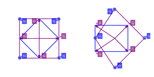
Figure 4. Polyhedral Velocity Sets: F0, F1 (left, right)

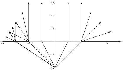
Figure 5. Polyhedral Velocity Sets: Raycast Solutions

When $\Pi_{\Sigma}(\mathbf{x}_{1})<-1$ there is no unique solution. For $\mathbf{x}_{1}=(-2,1)$ the algorithm halts in two steps at $y^{\text{ref}}=-1.5$, the first solution it reaches in this region. When $-1\leq\Pi_{\Sigma}(\mathbf{x}_{1})\leq 1$ it can be shown that the optimal crossing point is $\Pi_{\Sigma}(\mathbf{x}_{1})$. In this case the algorithm continuously bisects until it reaches $\varepsilon$ of the optimal solution. Figure 6 shows convergence when $\mathbf{x}_{1}=(0.5,1)$ and $y^{\text{ref}}=0.5$.

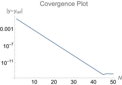
Figure 6. Polyhedral Velocity Sets: Convergence Plot

5. Conclusion

We have presented a bisection algorithm to solve the Elvis problem for general convex velocity sets. Then we proved the convergence of the algorithm with a linear rate. We then showed on the case of elliptical velocity sets that the proved convergence rate is optimal. Finally, we applied the algorithm with non-smooth velocity sets.

Future work include generalizing this algorithm to $n$ space dimensions. Also, a more efficient algorithm could be design on the model of the Newton–Raphson method to obtain quadratic convergence. However, that will require the use of second order optimality conditions which are not common in convex analysis.

Code availability

The algorithm has been implemented in Mathematica and is available at https://github.com/clintg105/Elvis-Trajectory-Optimization.git.