Free-Floating planet Mass Function from MOA-II 9-year survey towards the Galactic Bulge

Abstract

We present the first measurement of the mass function of free-floating planets (FFP) or very wide orbit planets down to an Earth mass, from the MOA-II microlensing survey in 2006-2014. Six events are likely to be due to planets with Einstein radius crossing times, $t_{\rm E}<0.5$days, and the shortest has $t_{\rm E}=0.057\pm 0.016$days and an angular Einstein radius of $\theta_{\rm E}=0.90\pm 0.14\mu$as. We measure the detection efficiency depending on both $t_{\rm E}$ and $\theta_{\rm E}$ with image level simulations for the first time. These short events are well modeled by a power-law mass function, $dN_{4}/d\log M=(2.18^{+0.52}_{-1.40})\times(M/8\,M_{\earth})^{-\alpha_{4}}$ dex^-1star^-1 with $\alpha_{4}=0.96^{+0.47}_{-0.27}$ for $M/M_{\odot}<0.02$. This implies a total of $f=21^{+23}_{-13}$ FFP or very wide orbit planets of mass $0.33<M/M_{\earth}<6660$ per star, with a total mass of $80^{+73}_{-47}M_{\earth}$ per star. The number of FFPs is $19_{-13}^{+23}$ times the number of planets in wide orbits (beyond the snow line), while the total masses are of the same order. This suggests that the FFPs have been ejected from bound planetary systems that may have had an initial mass function with a power-law index of $\alpha\sim 0.9$, which would imply a total mass of $171_{-52}^{+80}M_{\earth}$ star^-1. This model predicts that Roman Space Telescope will detect $988^{+1848}_{-566}$ FFPs with masses down to that of Mars (including $575^{+1733}_{-424}$ with $0.1\leq M/M_{\earth}\leq 1$). The Sumi et al. (2011) large Jupiter-mass FFP population is excluded.

1 Introduction

Gravitational microlensing observations toward the Galactic bulge (Galactic Bulge) enable exoplanet searches (Mao & Paczyński, 1991; Gaudi et al., 2008; Bennett et al., 2010; Suzuki et al., 2016; Koshimoto et al., 2021b), and the measurement of the stellar and sub-stellar mass functions (MFs) (Paczyński, 1991; Sumi et al., 2011; Mróz et al., 2017, 2019, 2020a).

Sumi et al. (2011) first interpreted the detection of short Einstein radius crossing time ($0.5<t_{\rm E}/{\rm day}<2$) microlensing events as evidence for the existence of a population of free-floating planets (FFP) and/or wide orbit planets. While that analysis was limited by the small number of events found in a 2 year subset of the survey by the Microlensing Observation in Astrophysics (MOA) group (Sumi et al., 2003) in collaboration with Optical Gravitational Lensing Experiment (OGLE) (Udalski et al., 1994), it opened up the field of FFP studies using microlensing.

Mróz et al. (2017) extended the work by using a larger sample from 5 years of the OGLE survey. They discovered 6 events with timescales shorter ($t_{\rm E}\sim 0.2$ day) than those in the previous work. These events are separated from the longer events by a gap around $t_{\rm E}\sim 0.5$ day which implying the possibility of a several Earth-mass FFP population.

These studies are based on distribution of $t_{\rm E}$, in which $t_{\rm E}$ is proportional to the square root of the lens mass $M$ as follows,

$$\begin{split}t_{\rm E}&=\frac{\sqrt{\kappa M\pi_{\rm rel}}}{\mu_{\rm rel}}\\ &=0.1\,{\rm day}\left(\frac{M}{5M_{\earth}}\right)^{1/2}\left(\frac{\pi_{\rm rel}}{18\mu\rm as}\right)^{1/2}\left(\frac{\mu_{\rm rel}}{5\rm mas\,yr^{-1}}\right)^{-1}.\end{split}$$ (1)

Here, $\kappa=4G/(c^{2}{\rm au})=8.144{\rm mas}/M_{\odot}$ and we expect $t_{\rm E}\sim 0.1$ day assuming typical value of the lens-source relative parallax: $\pi_{\rm rel}=\pi_{\rm l}^{-1}-\pi_{\rm s}^{-1}=1$ au$(D_{\rm l}^{-1}-D_{\rm s}^{-1})=18\mu$as for the bulge lens and a typical value of the lens-source relative proper motion in the direction of the Galactic center of $\mu_{\rm rel}=5$ mas yr^-1. The lens mass $M$, the distance $D_{\rm l}$ to the lens and the relative proper motion $\mu_{\rm rel}$ are degenerate in the observable $t_{\rm E}$. ($D_{s}$ is the distance to the source star.) This means that the mass function of the lens population has to be determined statistically, assuming a model of the star population density and velocities in the Galaxy.

Mróz et al. (2018) found the first short ($t_{\rm E}=0.32$ day) event showing the Finite Source (FS) effect, i.e., a finite source and a single point lens (FSPL), in which one can measure a FS parameter $\rho=\theta_{*}/\theta_{\rm E}$. Here $\theta_{*}$ is the angler source radius which can be estimated from an empirical relation with the source magnitude and color. The $\theta_{\rm E}$ is an angular Einstein radius given by

$$\theta_{\rm E}=\frac{\mu_{\rm rel}}{t_{\rm E}}=\sqrt{\kappa M\pi_{\rm rel}}.$$ (2)

This value of $\theta_{\rm E}$ can give us an inferred mass of the lens with better accuracy as we can eliminate one of the three-fold degenerate terms which affect $t_{\rm E}$, namely, $\mu_{\rm rel}$:

$$M=\frac{\theta_{\rm E}^{2}}{\kappa\pi_{\rm rel}}=5M_{\earth}\left(\frac{\theta_{\rm E}}{1.5\mu\rm as}\right)^{2}\left(\frac{\pi_{\rm rel}}{18\mu\rm as}\right)^{-1}.$$ (3)

While the inclusion of the angular Einstein radius, $\theta_{E}$, enables tighter constraints on the lens masses, it adds a complication to a statistical analysis of FFP properties because the microlensing event detection efficiency depends on both $t_{E}$ and $\theta_{E}$ (or equivalently $t_{E}$ and $\rho$).

So far, six short FSPL events have been discovered (Mróz et al., 2018, 2019b, 2020b, 2020c; Kim et al., 2021; Ryu et al., 2021). All of these have $\theta_{\rm E}<10\,\mu$as, implying that their lenses are most likely of planetary mass. All of these sources are red giants with the exception of the sub-giant source for OGLE-2016-BLG-1928 because their angular radii, i.e., cross-section, are significantly larger than main sequence stars.

Mróz et al. (2020b) found the short FSPL event, OGLE-2016-BLG-1928, with the smallest value of $\theta_{\rm E}=0.842\pm 0.064\mu$as to date. Its lens is the first terrestrial mass FFP candidate and the first evidence of such a population.

Kim et al. (2021) began a new approach to probing the FFP population by focusing on analyzing the $\theta_{\rm E}$ distribution in events with giant sources. Ryu et al. (2021) found a gap at $10<\theta_{\rm E}/\mu{\rm as}<30$ in the cumulative $\theta_{\rm E}$ distribution, which suggests a separation between the planetary mass population and other known populations, like brown dwarfs.

Gould et al. (2022) completed the analysis of 29 FSPL giant-source events found in the 2016-2019 KMTNet survey. They presented the $\theta_{\rm E}$ distributions down to $\theta_{\rm E}=4.35\,\mu$as and confirmed that there is a clear gap in the distribution of $\theta_{\rm E}$ at $9<\theta_{\rm E}/\mu{\rm as}<26$. They note that it is consistent with the gap in the $t_{\rm E}$ distribution shown by Mróz et al. (2017), indicating the existence of the low mass FFP population. They used what they refer to as a “relative detection efficiency” that depends only on $\theta_{\rm E}$, but not $t_{\rm E}$, to model the $\theta_{\rm E}$ distribution with a power law MF for the FFP and found $dN_{\rm FFP}/d\log M=(0.4\pm 0.2)(M/38M_{\earth})^{-p}$ dex^-1 star^-1, using a power law with $0.9\lesssim p\lesssim 1.2$. This range of the power, $p$, was estimated based on consideration of possible formation mechanisms, rather than a measurement. This would imply that the number of FFPs is at least an order of magnitude larger than the number of known bound planets.

We note that the Gould et al. (2022) result cannot be considered a measurement for a the following reasons. First, the true detection efficiency depends on both $t_{\rm E}$ and $\theta_{\rm E}$, and it is difficult to see how any selection criteria could remove the $t_{\rm E}$ dependence. As we discuss below in Section 4.1.1 and in K23 one can integrate over the $t_{\rm E}$ dependence of the detection efficiency to obtain an integrated detection efficiency. However, the integration over short $t_{\rm E}$ values depends on the FFP mass function. However, Gould et al. (2022) seem to avoid this difficulty by simply adopting an analytic formula for the “relative detection efficiency” depending only on $\theta_{\rm E}$. The Gould et al. (2022) paper gives no justification for this analytic formula.

In this paper, we present the distributions $\theta_{\rm E}$ and $t_{\rm E}$ values for the microlensing events toward the Galactic Bulge from 9 years of the MOA-II survey. We also present the first measurement of MF of the planetary mass objects using the $t_{\rm E}$ distribution. We describe the data in section § 2. We show the $\theta_{\rm E}$ distribution in section § 3. We present the $t_{\rm E}$ distribution and the best-fit MF in § 4. The discussion and conclusions are given in section § 5, and we compare the integrated detection efficiency in Appendix A.

2 Data

We use the microlensing sample selected from the MOA-II high cadence photometric survey toward the Galactic Bulge in the 2006-2014 seasons (Koshimoto et al., 2023, hereafter K23). MOA-II uses the 1.8-m MOA-II telescope which has a 2.18 deg² field of view (FOV) and which is located at the Mt. John University Observatory, New Zealand.

K23 used an analysis method similar to what was used by Sumi et al. (2011, 2013), but includes a correction of systematic errors and takes into account the finite source effect. They applied a de-trending code to all light curves to remove the systematic errors that correlate with seeing and airmass due to differential refraction, differential extinction and relative proper motion of stars in the same way as in Bennett et al. (2012) and Sumi et al. (2016). These corrections are important as they result in higher confidence in the light curve fitting parameters.

K23 selected light curves with a single instantaneous brightening episode and a flat constant baseline, which can be well fit with a point-source point-lens (PSPL) microlensing model (Paczyński, 1986). In addition to PSPL, they modeled the events with a FSPL model (Bozza et al., 2018), which is especially important for short events. These are the major improvements compared to the previous analysis in Sumi et al. (2011, 2013) in addition to the extension of the survey duration.

Although they identified 6,111 microlensing candidates, they selected only 3,554 and 3,535 objects as the statistical sample using the two relatively strict criteria CR1 and CR2, respectively. Here, CR2 was defined as the stricter criteria compared to their nominal criteria CR1 to check the effect of the choice of the criteria on a statistical study. These strict criteria ensure that $t_{\rm E}$ is well constrained for each event and reject any contamination.

Sumi et al. (2011) reported 10 short events with $t_{\rm E}<2$ days in the 2006-2007 dataset. Only 5 and 4 events survived following the application of CR1 and CR2, respectively. This is because the fitting results changed due to the re-reduction of the dataset. On the other hand, two events are newly found resulting 7 and 6 events following the application of CR1 and CR2, respectively. As a result, the excess at $t_{\rm E}=0.5-2$ day in the $t_{\rm E}$ distribution is not significant anymore, however, an even shorter event MOA-9y-6057 ($t_{\rm E}=0.22\pm 0.06$ day) is added.

Table 1: Comparison of parameters of short FS events with known FFP candidates.

field-chip-sub-ID	$t_{\rm E}$	$\rho$	$I_{\rm s,0}$	$\theta_{*}$	$\theta_{\rm E}$	reference
	$(\rm day)$		${(\rm mag)}$	($\mu$as)	($\mu$as)
MOA-9y-5919	0.057 $\pm$ 0.016	1.40 $\pm$ 0.46	17.23	1.26 $\pm$ 0.48	0.90 $\pm$ 0.14	K23
MOA-9y-770	0.315 $\pm$ 0.017	1.08 $\pm$ 0.07	14.71	5.13 $\pm$ 0.86	4.73 $\pm$ 0.75	K23
OGLE-2016-BLG-1928	0.0288 ${}_{-0.0016}^{+0.0024}$	3.39${}_{-0.11}^{+0.10}$	15.78	2.85 $\pm$ 0.20	0.842 $\pm$ 0.064	Mróz et al. (2020b)
KMT-2019-BLG-2073	0.272 $\pm$ 0.007	1.138 $\pm$ 0.012	14.45	5.43 $\pm$ 0.17	4.77 $\pm$ 0.19	Kim et al. (2021)
KMT-2017-BLG-2820	0.288 $\pm$ 0.015	1.096 $\pm$ 0.079	14.31	7.05 $\pm$ 0.44	5.94 $\pm$ 0.37	Ryu et al. (2021)
OGLE-2012-BLG-1323	0.155 $\pm$ 0.005	5.03 $\pm$ 0.07	14.09	11.9 $\pm$ 0.5	2.37 $\pm$ 0.10	Mróz et al. (2019b)
OGLE-2016-BLG-1540	0.320 $\pm$ 0.003	$1.65\pm 0.01$	13.51	15.1 $\pm$ 0.8	9.2 $\pm$ 0.5	Mróz et al. (2018)
OGLE-2019-BLG-0551	0.381 $\pm$ 0.017	4.49 $\pm$ 0.15	12.61	19.5 $\pm$ 1.6	4.35 $\pm$ 0.34	Mróz et al. (2020c)
MOA-9y-1944	1.594 $\pm$ 0.136	0.00928 $\pm$ 0.00032	20.14	0.43 $\pm$ 0.10	46.1 $\pm$ 10.5	K23
OGLE-2017-BLG-0560	0.905 $\pm$ 0.005	0.901 $\pm$ 0.005	12.47	34.9 $\pm$ 1.5	38.7 $\pm$ 1.6	Mróz et al. (2019b)

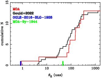
Figure 1: Observed cumulative distribution of $\theta_{\rm E}$ for 13 FSPL events from MOA (red line) and 29 FSPL events from KMTNet (black line) (Gould et al., 2022). The blue line indicates $\theta_{\rm E}=0.842\pm 0.064$ of terrestrial mass FFP candidate, OGLE-2016-BLG-1928 (Mróz et al., 2020b).

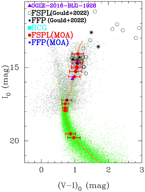
Figure 2: Extinction free CMD of gb3-7-6. The orange curve is the isochrone matched to this subfield. The cyan square is the RCG centroid. The red circles with error bars are sources of the 13 FSPL events in this work. The blue filled circles indicates the 2 FFP candidates in this work. The black open and filled circles are FSPL events and FFP events from Gould et al. (2022), respectively. The purple triangle indicates the source of terrestrial FFP, OGLE-2016-BLG-1928S (Mróz et al., 2020b).

3 Angular Einstein radius distribution

There are 13 FSPL events with $\theta_{\rm E}$ measurements in the sample, including two FFP candidates, MOA-9y-5919 and MOA-9y-770, that have terrestrial and Neptune masses, respectively. See K23 for the light curves and detailed parameters of the 13 events.

The red line in Figure 1 indicates the cumulative distribution of $\theta_{\rm E}$ from Table 7 of K23. The black line indicates the distribution of 29 FFPs by Gould et al. (2022) normalized to 13 events as a comparison. Although these can not be directly compared because these are not corrected for detection efficiencies, the general trends seen Figure 1 may give us some insights.

The distributions are consistent for $\theta_{\rm E}>30$ $\mu$as, where the effect of the detection efficiencies are likely small. There is a gap around $5<\theta_{\rm E}/{\rm\mu as}<70$ which is roughly consistent with the gap at $10<\theta_{\rm E}/{\rm\mu as}<30$ found by Ryu et al. (2021) and Gould et al. (2022). This gap confirmed the existence of the planetary mass population as distinct and separated from the stellar/brown dwarf population as indicated by Gould et al. (2022).

The MOA cumulative distribution shows fewer events over $30<\theta_{\rm E}/{\rm\mu as}<70$ compared to Gould et al. (2022). This may be just due to the small number of statistics. But note that K23 found a brown dwarf candidate MOA-9y-1944 with $\theta_{\rm E}=46.1\pm 10.5\,{\rm\mu as}$ although this is not in the final sample for statistical analysis because the source magnitude of $I_{\rm s}=21.91$ mag is fainter than the threshold of $I_{\rm s}<21.4$ mag.

In our sample, there is one event with a very small value of $\theta_{\rm E}$ of $0.90\pm 0.14$ $\mu$as. This confirms the existence of the terrestrial mass population which gives rise to events such as OGLE-2016-BLG-1928 which has $\theta_{\rm E}=0.842\pm 0.064$ (Mróz et al., 2020b). These values are significantly smaller than the lower edge of $\theta_{\rm E}\sim 4.35$ $\mu$as as reported in Gould et al. (2022). This is partly a result of selection bias given that Gould et al. (2022) focused on the sample with super-giant sources, see Figure 2.

We compare the parameters of these events to six known FFP candidates with $\theta_{\rm E}$ measurements in Table 1. The sources of all known FFP candidates except OGLE-2016-BLG-1928 are red clump giants (RCGs) or red super-giants which have large $\theta_{\rm*}=5.4,7.1,11.9,15.1,19.5$ and $34.9$ $\mu$as. The magnification tend to be suppressed by large $\theta_{\rm*}$ with small $\theta_{\rm E}$, i.e., large $\rho$ as $A_{\rm FS,max}=\sqrt{1+4/\rho^{2}}$ $(\rho>1)$ (Maeder, 1973; Agol, 2003; Riffeser et al., 2006). For example, in case of the terrestrial mass lens with $\theta_{\rm E}\sim 1\mu$as, the maximum magnification will be only $A_{\rm FS,max}=1.066,1.039,1.014,1.009,1.005$ and $1.002$ for the above values of $\theta_{\rm*}$, respectively. Note that the source of the terrestrial FFP candidate event, OGLE-2016-BLG-1928S is a sub-giant with $\theta_{\rm*}=2.37$ $\mu$as. It is important to search for short FSPL with sub-giants and dwarf sources to find low mass FFP. There is no FSPL event with a red super-giant source in our sample because these are saturated in MOA image data.

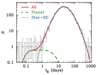
Figure 3: The observed timescale $t_{\rm E}$ distribution passing criteria CR2 from the 9 year MOA-II survey. The 1-$\sigma$ error bars and upper limits are based on the poisson distribution. The red line indicates the best fit single lens model for all population. The blue dotted line represents the known populations of stars, brown dwarfs, and stellar remnants, and the green dashed line represents the planetary mass population.

4 Likelihood analysis of mass function

In the final sample of K23, there are 10 (12) short timescale events with $t_{\rm E}<1$ day after applying CR2 (CR1). Figure 3 shows the $t_{\rm E}$ distribution of the CR2 sample. The distribution is roughly symmetric in $\log t_{\rm E}$, with a tail at $t_{\rm E}<0.5$. This confirmed the existence of such short timescale events with $t_{\rm E}<0.5$ day as reported by Mróz et al. (2017). In this section, we perform a likelihood analysis on each of the 3554 (CR1) and 3535 (CR2) events using a Galaxy model to constrain the mass function of lens objects.

We define the likelihood, ${\cal L}$, in Section 4.1. In Sections 4.2 and 4.3, we determine the mass function without and with a planetary mass population, respectively, by minimizing $\chi^{2}\equiv-2\ln{\cal L}$. Although the absolute value of $\chi^{2}$ is not meaningful due to its dependence on an arbitrary normalization associated with our likelihood calculation, the fitting procedure is still statistically valid as the relative likelihood between two models, represented by $\Delta\chi^{2}$, is independent of the normalization.

Note that results of the likelihood analysis for sample CR1 and CR2 are very similar. In the following sections, we show only the results for CR2 as our final results except in the tables.

4.1 Likelihood

Although our sample contains more than 3500 events, the mass function of planetary-mass objects is largely determined by the events with $t_{\rm E}<1$ day, which account for about 0.3% of these events. We define two likelihoods: ${\cal L}_{\rm short}$ for short timescale events with the best-fit $t_{\rm E}<1$ day, and ${\cal L}_{\rm long}$ for events with the best-fit $t_{\rm E}\geq 1~{}{\rm day}$. In our likelihood analysis, we use the combined likelihood ${\cal L}={\cal L}_{\rm short}{\cal L}_{\rm long}$.

For ${\cal L}_{\rm long}$, we simply use the best-fit $t_{\rm E}$ values provided by K23, which is similar to the approach by previous studies (Sumi et al., 2011; Mróz et al., 2017). This is because of (i) the relatively small uncertainties in $t_{\rm E}$, (ii) the effect of individual $t_{\rm E}$ uncertainties is statistically marginalized by the large number of events, (iii) the limited sensitivity to $\theta_{\rm E}$, and (iv) the minimal impact on our primary goal of measuring the mass function of planetary mass objects.

On the other hand, the situation is the opposite for the short events, ${\cal L}_{\rm short}$. That is: (i) the $t_{\rm E}$ uncertainties are relatively large due to their shorter magnification period but they must be smaller than the event selection threshold listed in Table 2 of K23, (ii) the number of events is very limited (12 for CR1 and 10 for CR2), and $t_{\rm E}<$ 1 day range is only sparsely covered in Figure 3. Thus, the number of $t_{\rm E}<$ 1 day events may not be sufficient to statistically marginalize the effect of $t_{\rm E}$ uncertainties of individual events in the likelihood analysis, (iii) because the $\rho=\theta_{*}/\theta_{\rm E}$ values are generally much larger than those of longer timescale events, one may get beneficial constraints on $\theta_{\rm E}$ even when the $\theta_{\rm E}$ values are not well determined, and (iv) they play a crucial role in determining the mass function of planetary mass objects. Therefore, we must use the joint probability distribution of $(t_{\rm E},\theta_{\rm E})$ for each event derived by K23 using the Markov Chain Monte Carlo (MCMC) method for ${\cal L}_{\rm short}$. However, the $(t_{\rm E},\theta_{\rm E})$ probability distributions for each event depends on the FFP mass function that we are trying to measure, while the event detection efficiency also depends on both $t_{\rm E}$ and $\theta_{\rm E}$. So, the probability distribution for the $t_{\rm E}$ and $\theta_{\rm E}$ values for each event depends upon both the light curve data and the FFP mass function. Rather than running our light curve model MCMC calculations for the short events separately for every mass function model we consider, we simplify our calculations by using the ‘importance sampling” method of Monte Carlo integration (Press et al., 1992). This means that we run the MCMC light curve models with weighting of the $\log t_{\rm E}$ and $\log\theta_{\rm E}$ distributions given by an uninformative (and incorrect) “prior,” $p_{0}(\log t_{\rm E},\log\theta_{\rm E})$ that is uniform in both $\log t_{\rm E}$ and $\log\theta_{\rm E}$. A function like $p_{0}(\log t_{\rm E},\log\theta_{\rm E})$ is sometimes called an “interim prior” (Foreman-Mackey et al., 2014), but we have not used it as a Bayesian prior. Instead, we replace $p_{0}(\log t_{\rm E},\log\theta_{\rm E})$ with the correct distribution over $\log t_{\rm E}$ and $\log\theta_{\rm E}$ for each mass function model in our FFP mass function likelihood calculation. The only Bayesian prior assumptions assumed in this analysis are the Galactic model assumptions discussed in Section 4.2 and the mass function model priors discussed in Section 4.3 .

We describe the simpler likelihood function for the long duration events, ${\cal L}_{\rm long}$, in Section 4.1.1, and then we describe ${\cal L}_{\rm short}$ in Section 4.1.2.

4.1.1 Likelihood for events with $t_{\rm E}\geq 1$ day

We define the likelihood for events with $t_{\rm E}\geq 1$ day by

$${\cal L}_{\rm long}\propto\prod_{i=1}^{N_{\rm long}}{\cal G}(t_{{\rm E},i};\Gamma),$$ (4)

where $i$ runs over all the $N_{\rm long}$ events that have the best-fit $t_{\rm E}\geq 1$ day in our sample ($N_{\rm long}=3542$ for CR1 and $N_{\rm long}=3525$ for CR2), and $t_{{\rm E},i}$ is the best-fit $t_{\rm E}$ value for $i$th event given by K23.

The function ${\cal G}(t_{\rm E};\Gamma)$ is the model’s detectable event rate as a function of $t_{\rm E}$ with given model event rate $\Gamma$, combined for the 20 survey fields, given by

$${\cal G}(t_{\rm E};\Gamma)=\sum_{j}w_{j}\,g_{j}(t_{\rm E};\Gamma_{j}).$$ (5)

Here, $j$ takes field index values gb1 to gb21, except for gb6. See Table 1 of K23 for the location and properties of each field. The weight $w_{j}$ for the $j$th field is given by

$$w_{j}=\sum_{k\in j}n_{{\rm RC},k}^{2}f_{{\rm LF},k},$$ (6)

where $k$ indicates a 1024 pixel $\times$ 1024 pixel subframe in the $j$th field ($k=1,2,...,80$), $n_{{\rm RC},k}$ is the number density of RCGs in the $k$th subfield, $f_{{\rm LF},k}$ is the fraction of stars with magnitude $I<21.4$ mag in the $k$th subfield, and $w_{j}$ is thus proportional to the expected event rate in the $j$th field. To calculate $f_{{\rm LF},k}$, we used a combined luminosity function that uses the OGLE-III photometry map (Szymański, 2011) for bright stars and the Hubble Space Telescope data by (Holtzman et al., 1998) for faint stars.

The function $g_{j}$ is the model’s detectable event rate as a function of $t_{\rm E}$ for field $j$ as given by

$$g_{j}(t_{\rm E};\Gamma_{j}) =\tilde{\epsilon}_{j}(t_{\rm E};\Gamma_{j})\,\Gamma_{j}(t_{\rm E}),$$ (7)

where $\tilde{\epsilon}(t_{\rm E};\Gamma)$ is the integrated detection efficiency of the survey as a function of $t_{\rm E}$. K23 demonstrated that when finite source effects are important, the detection efficiency, $\epsilon(t_{\rm E},\theta_{\rm E})$ is a function of two variables, $t_{\rm E}$ and $\theta_{\rm E}$. Therefore, we must integrate over $\theta_{\rm E}$ to obtain the integrated detection efficiency, $\tilde{\epsilon}(t_{\rm E};\Gamma)$, which now depends upon the event rate and the mass function of the lens objects. This gives

$$\tilde{\epsilon}_{j}(t_{\rm E};\Gamma)=\int_{\theta_{\rm E}}\epsilon_{j}(t_{\rm E},\theta_{\rm E})\,\Gamma_{j}(\theta_{\rm E}|t_{\rm E})d\theta_{\rm E},$$ (8)

where $\epsilon_{j}(t_{\rm E},\theta_{\rm E})$ is the detection efficiency for events with $t_{\rm E}$ and $\theta_{\rm E}$ for $i$th field. We use the detection efficiency $\epsilon_{j}(t_{\rm E},\theta_{\rm E})$ estimated by the image level simulations in K23 for the 20 fields of the MOA-II 9-yr survey.

We consider the model event rate as functions of $t_{\rm E}$ and $(t_{\rm E},\theta_{\rm E})$, denoted by $\Gamma(t_{\rm E})$ and $\Gamma(t_{\rm E},\theta_{\rm E})$, respectively. These are normalized functions so that their integrations give one, i.e., these are probability density functions of $t_{\rm E}$ and $(t_{\rm E},\theta_{\rm E})$, respectively. $\Gamma(\theta_{\rm E}|t_{\rm E})=\Gamma(t_{\rm E},\theta_{\rm E})/\Gamma(t_{\rm E})$ is the probability density of events with $\theta_{\rm E}$ given $t_{\rm E}$. Thus, the calculation of $\tilde{\epsilon}(t_{\rm E};\Gamma)$ in Eq. (8) has to be done for every proposed MF during the fitting procedure because $\Gamma(\theta_{\rm E}|t_{\rm E})$ depends on the MF.

The function $\Gamma_{j}(t_{\rm E},\theta_{\rm E})$ for $j$th field can be separated from the MF (Han & Gould, 1996),

$$\Gamma_{j}(t_{\rm E},\theta_{\rm E})=\int\gamma_{j}(t_{\rm E}M^{-1/2},\theta_{\rm E}M^{-1/2})\Phi(M)\sqrt{M}dM,$$ (9)

where $\gamma_{j}(t_{\rm E},\theta_{\rm E})$ is the event rate for lenses with mass $1\,M_{\sun}$ and $\Phi(M)$ is the present-day MF (expressed as $dN/dM$). Although substituting Eqs. (8) and (9) makes the calculation of $g_{j}(t_{\rm E};\Gamma_{j})$ in Eq. (7) a double integral over $M$ and $\theta_{\rm E}$, K23 showed that the integration over $\theta_{\rm E}$ is largely avoidable during a fitting procedure by switching the order of the integrals and calculating the integral over $\theta_{\rm E}$ before the fitting.

We calculate $\gamma_{j}(t_{\rm E},\theta_{\rm E})$ for each field using the density and velocity distribution of stars from the latest parametric Galactic model toward the Galactic Bulge based on Gaia and microlensing data (Koshimoto et al., 2021a).

Figure 4 shows the integrated detection efficiencies $\tilde{\epsilon}(t_{\rm E};\Gamma)$ for the event rate calculated with the best fit MF model with the criteria CR2. The curve for CR1 is similar. This detection efficiency is about a factor two lower than that of Mróz et al. (2017) at the low end around $t_{\rm E}=0.1$ days even for the similar cadence of the survey. The main reason is likely that Mróz et al. (2017) did not include the finite source effect in their simulation. Koshimoto et al. (2023) confirmed that this difference is about a factor two at $t_{\rm E}=0.1$ days by the simulation in their Figure 7.

Note that detection efficiencies at short $t_{\rm E}$ with $\rho>1$ may be improved in a future analysis. For events with $\rho>1$, the magnification can be significant with the minimum impact parameter up to $u_{\rm 0}\lesssim\rho$. This is likely to be more important for bright giant sources because these have higher S/N ratio even at low magnification (see also Appendix A) . However such events are rejected by the criterion $u_{\rm 0}\leq 1$ in K23. This criterion is applied because it is useful to robustly remove the various artifacts and keep the sample as clean as possible. This may be improved in a future analysis with a more careful investigation.

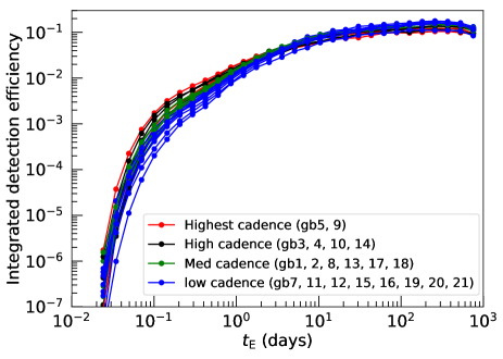
Figure 4: Integrated detection efficiencies, $\tilde{\epsilon}(t_{\rm E};\Gamma)$, as a function of the timescale $t_{\rm E}$ down to the source magnitude of $I_{\rm s}<21.4$ mag for the criteria CR2. Red, black, green and blue lines indicate the efficiencies of fields with the highest, high, medium and low cadence, respectively.

4.1.2 Likelihood for short timescale ($t_{\rm E}<1$ day) events

We follow the importance sampling method used by Hogg et al. (2010) to convert the the uninformative “interim prior”, $p_{0}(\log t_{\rm E},\log\theta_{\rm E})$ used for the the light curve MCMC for each event, to a probability distribution for event $i$, ${\cal G}(\log t_{{\rm E},i},\log\theta_{{\rm E},i};\Gamma)$, that depends on the event rate for each mass function model, $\Gamma$. However, while Hogg et al. (2010) characterized their calculation as a modification of the assumed prior, based on the data, this in not the case for our analysis. Instead, we are replacing $p_{0}$ with the probability distribution implied by our mass function model, using the importance sampling Monte Carlo integration method (Press et al., 1992). We use the probability distribution for each event from its MCMC analysis to calculate the likelihood for the short timescale events, ${\cal L}_{\rm short}$. Given the output MCMC samples of posterior distributions for individual events by K23, the likelihood is given by

$${\cal L}_{\rm short}\propto\prod_{i=1}^{N_{\rm short}}\sum_{k=1}^{K_{i}}\frac{{\cal G}(\log t_{{\rm E},ik},\log\theta_{{\rm E},ik};\Gamma)}{p_{0}(\log t_{{\rm E},ik},\log\theta_{{\rm E},ik})},$$ (10)

where $i$ runs over all the $N_{\rm short}$ events that have the best-fit $t_{\rm E}<1$ day ($N_{\rm short}=12$ for CR1 and $N_{\rm short}=10$ for CR2), $k$ runs over all the $K_{i}$ samples in the MCMC sample of the probability distribution for $i$th event, and $p_{0}(\log t_{\rm E},\log\theta_{\rm E})$ is the uninformative prior distribution used for these MCMC calculations. The model’s detectable event rate as a function of $(\log t_{\rm E},\log\theta_{\rm E})$ is given by

$${\cal G}(\log t_{\rm E},\log\theta_{\rm E};\Gamma)=\sum_{j}w_{j}\,g_{j}(\log t_{\rm E},\log\theta_{\rm E};\Gamma_{j})$$ (11)

with

$$g_{j}(\log t_{\rm E},\log\theta_{\rm E};\Gamma_{j})=\epsilon_{j}(\log t_{\rm E},\log\theta_{\rm E})\,\Gamma_{j}(\log t_{\rm E},\log\theta_{\rm E}),$$ (12)

where we represented it as a function of $(\log t_{\rm E},\log\theta_{\rm E})$ rather than $(t_{\rm E},\theta_{\rm E})$ because the MCMC calculations of K23 provide the probability distributions based on the uninformative uniform prior in $(\log t_{\rm E},\log\theta_{\rm E})$, i.e., $p_{0}(\log t_{\rm E},\log\theta_{\rm E})={\rm const.}$.

Eq. (10) calculates the likelihood by summing the ratio of ${\cal G}(\log t_{\rm E},\log\theta_{\rm E};\Gamma)$ to $p_{0}(\log t_{\rm E},\log\theta_{\rm E})$ to replace the uniform prior (i.e., $p_{0}$), used for the MCMC calculations with the new probability distribution (i.e., ${\cal G}$) that depends on our mass function model. This method, which uses all the MCMC samples, allows ${\cal L}_{\rm short}$ to account for the uncertainty of the parameters, unlike ${\cal L}_{\rm long}$ given in Eq. (4).

Despite the significant computational cost of Eq. (10) associated with performing a summation over $K_{i}$ (typically $\sim 5\times 10^{5}$) samples for each proposed mass function during the fitting process, we addressed this by implementing a binning strategy for the MCMC sample using grids of $(\log t_{\rm E},\log\theta_{\rm E})$ with a size of (0.05 dex $\times$ 0.05 dex), which significantly increased the computational efficiency.

4.2 Mass function of known population

Firstly, we perform the likelihood analysis without the short events with $t_{\rm E}<1$ day using the Galactic model with the MF of known population, i.e., stellar remnants (black holes (BH), neutron stars (NS) and white dwarfs(WD)), main sequence stars (MS) and brown dwarfs (BD). We use a broken power-law MF given by

$$\frac{dN}{d\log M}\propto\left\{\begin{array}[]{ll}{M^{-\alpha_{1}}}&(M_{1}<M/M_{\sun}<120)\\ {M^{-\alpha_{2}}}&(0.08<M/M_{\sun}<M_{1})\\ {M^{-\alpha_{3}}}&(3\times 10^{-4}<M/M_{\sun}<0.08).\\ \end{array}\right.$$ (13)

We adopt the values of parameters $\alpha_{1}=1.32$ and $\alpha_{2}=0.13$, $\alpha_{3}=-0.82$ and $M_{1}=0.86$ from the E+E_X model of Koshimoto et al. (2021a) by default unless specified as fitting parameters in the following three models. The minimum mass $3\times 10^{-4}\,M_{\sun}$ is taken to be smaller than the theoretical minimum mass of the gas cloud, $\sim$Jupiter-mass, that collapses to form a brown dwarf (Boss et al., 2003). During our fitting procedure, a proposed initial mass function (IMF) is converted into a present-day mass function following the procedure used by Koshimoto et al. (2021a) that combines their stellar age distribution and the initial-final mass relation by Lam et al. (2020) to evolve stars into stellar remnants.

We consider three models here: BD1, BD2, and BD3. In BD1, we fit only $\alpha_{3}$ as a fitting parameter, while fixing $\alpha_{1}$, $\alpha_{2}$, and $M_{1}$. Similarly, in BD2, we fit $\alpha_{3}$ and $\alpha_{2}$, and in BD3, we fit $\alpha_{1}$, $\alpha_{2}$, $\alpha_{3}$, and $M_{1}$. To perform the fitting, we use the Markov Chain Monte Carlo (MCMC) method (Metropolis et al., 1953), and assign uniform distributions as priors for all the parameters.

The best fit models BD1, BD2 and BD3 are almost indistinguishable from the blue dotted line in Figure 3. One can see that the models fit the data with $t_{\rm E}>1$ day very well. The best fit parameters and $\chi^{2}$ values are listed in Table 2. There is no significant difference in the resultant parameters between different selection criteria or among the BD1, BD2, and BD3 models.

All of the parameters are consistent with those of Koshimoto et al. (2021a) within $1\sigma$. This indicates that our dataset confirmed the Galactic model and MF of known objects by Koshimoto et al. (2021a). This also indicates that our dataset is consistent with the OGLE-IV $t_{\rm E}$ distribution for $t_{\rm E}>1$ day (Mróz et al., 2017, 2019) that is fitted by Koshimoto et al. (2021a).

In the following analysis, we fit only $\alpha_{3}$ and fix all other parameters for the known populations. Note, in Koshimoto et al. (2021a), the Galactic model and MF are constrained to satisfy the microlensing $t_{\rm E}$ distribution, stellar number counts and the Galactic Bulge mass from other observations, simultaneously. In principle, the MF should not be changed alone because it is related to other parameters of the Galactic model. However, the contribution of objects with $M/M_{\sun}<0.08$ are negligible in stellar number counts and as a fraction of the Galactic Bulge mass. Thus, we assume that a model with a different slope at lower masses with $M/M_{\sun}<0.08$ is still valid.

Table 2: Best fit parameters of the mass function for known population.

model	BD1		BD2		BD3		Koshimoto+21a
	CR1	CR2	CR1	CR2	CR1	CR2
$M_{1}$	($0.86)$	($0.86)$	($0.86)$	($0.86)$	$0.97^{-0.04}_{-0.34}$	$0.99^{-0.06}_{-0.37}$	$0.86^{+0.09}_{-0.10}$
$\alpha_{1}$	($1.32)$	($1.32)$	($1.32)$	($1.32)$	$1.33^{+0.21}_{-0.17}$	$1.34^{+0.18}_{-0.18}$	$1.32^{+0.14}_{-0.10}$
$\alpha_{2}$	($0.13)$	($0.13)$	$0.20^{+0.07}_{-0.05}$	$0.20^{+0.07}_{-0.05}$	$0.23^{+0.04}_{-0.19}$	$0.24^{+0.04}_{-0.21}$	$0.13^{+0.11}_{-0.12}$
$\alpha_{3}$	$-0.60^{+0.08}_{-0.13}$	$-0.62^{+0.09}_{-0.14}$	$-0.74^{+0.13}_{-0.30}$	$-0.76^{+0.14}_{-0.30}$	$-0.76^{+0.19}_{-0.26}$	$-0.79^{+0.22}_{-0.25}$	$-0.82^{+0.24}_{-0.51}$
$\chi^{2}$	35919.4	35722.6	35918.2	35721.5	35918.0	35721.3

Note. — Some of the upper errors of $M_{1}$ is negative because the best fit value is outside of the 68% range. This is because $M_{1}$ is restricted to be less than 1 $M_{\sun}$.

4.3 Mass function of planetary mass population

If the candidates with $t_{\rm E}<0.5$ day are really due to microlensing, they can not be explained by known populations, i.e., stellar remnants, MS or BD. To explain the tail for short values of $t_{\rm E}$, we defined a new model “PL” which introduces a planetary mass population by the following power law in addition to known populations (Eq. 13),

$$\frac{dN_{4}}{d\log M}=Z\left(\frac{M}{M_{\rm norm}}\right)^{-\alpha_{4}},(M_{\rm min}<M/M_{\sun}<0.02).$$ (14)

Here $Z$ is a normalization factor and $M_{\rm norm}$ is a reference mass whose inclusion allows $Z$ to have a unit of (dex)^-1. Although $M_{\rm norm}$ can be an arbitrary zero point, we found that the uncertainty in $Z$ is minimized when we adopt $M_{\rm norm}=8\,M_{\earth}$ which is recognized as a pivot point.

In the model PL, we use $\alpha_{3}$, $\alpha_{4}$ and $Z$, as fitting parameters and fix parameters $\alpha_{1}=1.32$, $\alpha_{2}=0.13$ and $M_{1}=0.86$ (Koshimoto et al., 2021a). We assign uniform distributions as priors for $\alpha_{3}$, $\alpha_{4}$ and $\log Z$ in our MCMC run. We found that the fitting result does not depend on $M_{\rm min}$ at all when $M_{\rm min}<3\times 10^{-7}\,M_{\sun}$, which indicates our data sensitivity is down to $\sim 3\times 10^{-7}M_{\sun}$. Thus, we decided to use $M_{\rm min}=10^{-7}$.

The red solid line in Figure 3 represents the best fit model for all populations with the CR2 sample. This figure indicates that the model represents the observed $t_{\rm E}$ distribution well. Note that although the observed $t_{\rm E}$ distribution shown in black in Figure 3 does not include error bars along the $t_{\rm E}$ axis, the best-fit line is derived from our likelihood analysis that takes into account the $t_{\rm E}$ errors as well as the $\theta_{\rm E}$ constraints for the short events with $t_{\rm E}<1$ day. Figure 5 shows the posterior distributions of the parameters of PL model. The best fit parameters and $\chi^{2}$ are listed in Table 3.

The best fit power index for BD is $\alpha_{3}=-0.58^{+0.12}_{-0.16}$ which is consistent with the model without the planetary mass population.

The best fit MF of the planetary mass populations with the normalization $Z$ relative to stars (MS+BD+WD) (integrated IMF over $3\times 10^{-4}<M/M_{\sun}<8$) can be expressed as

$$\frac{dN_{4}}{d\log M}=\frac{2.18^{+0.52}_{-1.40}}{\rm dex\times star}\left(\frac{M}{8\,M_{\earth}}\right)^{-\alpha_{4}},$$ (15)

where $\alpha_{4}=0.96^{+0.47}_{-0.27}$. Figure 6 shows the IMF of the best fit PL model. This $\alpha_{4}$ is consistent with the corresponding power law index of $0.9\lesssim p\lesssim 1.2$ suggested by Gould et al. (2022).

This can be translated to the normalization per stellar mass of stars, $Z^{M_{\sun}}$, as,

$$\frac{dN_{4}}{d\log M}=\frac{5.48^{+1.18}_{-3.50}}{{\rm dex}\times M_{\sun}}\left(\frac{M}{8\,M_{\earth}}\right)^{-\alpha_{4}}.$$ (16)

This implies that the number of FFPs per stars is $f=21^{+23}_{-13}$ star^-1 over the mass range $10^{-6}<M/M_{\sun}<0.02$ ($0.33<M/M_{\earth}<6660$). Note that this value is vary depending on the minimum mass. The total mass of FFPs per star is $m=80^{+73}_{-47}M_{\earth}(0.25_{-0.15}^{+0.23}M_{\rm J})$ star^-1. This is less dependent from the minimum mass. The total mass of FFPs per $M_{\sun}$ is $m^{M_{\sun}}=202^{+166}_{-114}$ $M_{\earth}(0.64_{-0.11}^{+0.19}M_{\rm J})M_{\sun}^{-1}$. This is more robust values less dependent on uncertainty in the abundances of the low mass objects for both FFP and BD.

The normalization, number and total mass of FFP relative to MS+BD ($3\times 10^{-4}<M/M_{\sun}<1.1$) are also shown in Table 3. These normalizations can be translated to $Z_{\rm MS+BD}=0.53^{+0.19}_{-0.40}$ dex^-1star^-1 and $Z_{\rm MS+BD}^{M_{\sun}}=2.44^{+0.71}_{-1.82}$ dex${}^{-1}M_{\sun}^{-1}$ with $M_{\rm norm}=38M_{\earth}$. These are almost same as $Z_{\rm MS+BD}=0.39\pm 0.18$ dex^-1star^-1 and $Z_{\rm MS+BD}=1.96\pm 0.98$ dex${}^{-1}M_{\sun}^{-1}$ with $M_{\rm norm}=38M_{\earth}$ by Gould et al. (2022).

Note that the lenses for these short events could be either FFP or planets with very wide separations of more than about ten astronomical units (AU) from their host stars, for which we cannot detect the host star in the light curves.

Table 3: Best fit parameters of the mass function for the planetary mass population.

	CR1	CR2		Gould+22
($M_{\rm norm}$)	($8~{}M_{\earth}$)	($8~{}M_{\earth}$)	($38~{}M_{\earth}$)	($38~{}M_{\earth}$)
$M_{1}$	($0.86)$	($0.86)$
$\alpha_{1}$	($1.32)$	($1.32)$
$\alpha_{2}$	($0.13)$	($0.13)$
$\alpha_{3}$	$-0.55^{+0.13}_{-0.17}$	$-0.58^{+0.12}_{-0.16}$
$\alpha_{4}$	$0.90^{+0.48}_{-0.27}$	$0.96^{+0.47}_{-0.27}$		fixed at $0.9$ or $1.2$
$Z$	$2.08^{+0.54}_{-1.33}$	$2.18^{+0.52}_{-1.40}$	$0.49^{+0.17}_{-0.37}$
$Z_{\rm MS+BD}$	$2.27^{+0.60}_{-1.46}$	$2.38^{+0.58}_{-1.53}$	$0.53^{+0.19}_{-0.40}$	$0.39\pm 0.20\pm?$
$Z^{M_{\sun}}$	$5.33^{+1.26}_{-3.40}$	$5.48^{+1.18}_{-3.50}$	$1.22^{+0.35}_{-0.91}$
$Z^{M_{\sun}}_{\rm MS+BD}$	$10.63^{+2.52}_{-6.78}$	$10.95^{+2.36}_{-6.97}$	$2.44^{+0.71}_{-1.82}$	$1.96\pm 0.98\pm?$
$f$	$17^{+20}_{-11}$	$21^{+23}_{-13}$
$f_{\rm MS+BD}$	$19^{+22}_{-12}$	$23^{+25}_{-15}$
$f^{M_{\sun}}$	$45^{+54}_{-30}$	$53^{+59}_{-34}$
$f^{M_{\sun}}_{\rm MS+BD}$	$89^{+107}_{-59}$	$106^{+117}_{-68}$
$m$	$89^{+96}_{-56}M_{\earth}$	$80^{+73}_{-47}M_{\earth}$
$m_{\rm MS+BD}$	$98^{+107}_{-61}M_{\earth}$	$88^{+81}_{-51}M_{\earth}$
$m^{M_{\sun}}$	$229^{+219}_{-140}M_{\earth}$	$202^{+166}_{-114}M_{\earth}$
$m^{M_{\sun}}_{\rm MS+BD}$	$457^{+439}_{-279}M_{\earth}$	$404^{+333}_{-228}M_{\earth}$
$\chi^{2}$	36273.0	36024.1

Note. — We adopt the model for CR2 as the final result.

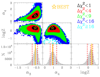
Figure 5: Posterior distributions of the parameters of the PL model for sample CR2. The vertical red dotted lines indicate the median and $\pm 1\sigma$. The vertical orange line indicates the best fit.

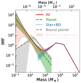
Figure 6: Initial mass function (IMF) of the best fit PL model for CR2. The red line indicates the best fit for all population. The blue dotted line and green dashed line show the IMFs for the stellar and brown dwarf population and for the planetary mass population, respectively. The shaded areas indicate $1\sigma$ error. The gray dashed-line and the shaded area indicate the best-fit and $1~{}\sigma$ range of the bound planet MF by Suzuki et al. (2016) via microlens. The pink shaded area indicate $1\sigma$ uncertainty for the broken power law FFP model.

4.4 Broken power law MF for the planetary mass population

In order to demonstrate the FFP mass function uncertainty at low masses, we have also modeled the planetary mass population with a broken power law MF given by

$$\frac{dN_{4}}{d\log M}\propto\left\{\begin{array}[]{ll}Z\left(\frac{M}{M_{\rm norm}}\right)^{-\alpha_{4}},&(M_{\rm br}<M/M_{\sun}<0.02)\\ M^{-\alpha_{5}},&(M_{\rm min}<M/M_{\sun}<M_{\rm br}).\\ \end{array}\right.$$ (17)

Here, $M_{\rm br}$ is a break mass and $\alpha_{5}$ is a power bellow $M_{\rm br}$. $M_{\rm min}=10^{-7}M_{\sun}$ is same as the previous section.

In Figure 6, we show the 1 $\sigma$ range of the broken power law PL model along with the best fit single power law MF given in the previous section for comparison. The median and 1 $\sigma$ range of the parameters and $\chi^{2}$ are listed in Table 4. The resultant broken power law MF is consistent with the single power law model while the uncertainty is larger. Although the MF is relatively well constrained down to an Earth mass, the uncertainty is much larger bellow an Earth mass. This is as expected because of our low sensitivity bellow to planets of less than an Earth mass.

This model implies that the number of FFPs per stars is $f=17^{+39}_{-12}$ star^-1 over the mass range $10^{-6}<M/M_{\sun}<0.02$ ($0.33<M/M_{\earth}<6660$). The total mass of FFPs per star is $m=69^{+107}_{-36}$ $M_{\earth}(0.22_{-0.11}^{+0.33}M_{\rm J})$ star^-1. The total mass of FFPs per $M_{\sun}$ is $m^{M_{\sun}}=175^{+246}_{-89}$ $M_{\earth}(0.55_{-0.28}^{+0.77}M_{\rm J})M_{\sun}^{-1}$. These numbers are also consistent with those for the single power law model but has larger uncertainties. This result is useful to see the conservative uncertainty of MF. In the following discussion, although we use only the results for the single power law model, the discussion is qualitatively same for the broken power law.

Table 4: Median and uncertainty of parameters of the broken power law mass function for the planetary mass population.

	CR1	CR2
($M_{\rm norm}$)	($8~{}M_{\earth}$)	($8~{}M_{\earth}$)
$\alpha_{3}$	$-0.54^{+0.12}_{-0.17}$	$-0.58^{+0.12}_{-0.19}$
$\alpha_{4}$	$1.07^{+0.93}_{-0.49}$	$1.14^{+0.97}_{-0.54}$
$\alpha_{5}$	$0.13^{+1.33}_{-3.07}$	$0.13^{+1.32}_{-3.10}$
$\log M_{\rm br}$	$-5.35^{+1.35}_{-1.02}$	$-5.27^{+1.28}_{-1.05}$
$Z$	$1.79^{+2.91}_{-1.08}$	$1.85^{+3.14}_{-1.17}$
$Z_{\rm MS+BD}$	$1.96^{+3.19}_{-1.18}$	$2.03^{+3.43}_{-1.28}$
$Z^{M_{\sun}}$	$4.57^{+7.54}_{-2.77}$	$4.62^{+7.92}_{-2.91}$
$Z^{M_{\sun}}_{\rm MS+BD}$	$9.12^{+15.05}_{-5.52}$	$9.22^{+15.79}_{-5.82}$
$f$	$15^{+36}_{-11}$	$17^{+39}_{-12}$
$f_{\rm MS+BD}$	$17^{+40}_{-12}$	$18^{+42}_{-13}$
$f^{M_{\sun}}$	$39^{+96}_{-28}$	$42^{+98}_{-30}$
$f^{M_{\sun}}_{\rm MS+BD}$	$79^{+191}_{-57}$	$85^{+196}_{-61}$
$m$	$73^{+119}_{-40}$	$69^{+107}_{-36}$
$m_{\rm MS+BD}$	$80^{+131}_{-44}$	$75^{+118}_{-39}$
$m^{M_{\sun}}$	$192^{+275}_{-103}$	$175^{+246}_{-89}$
$m^{M_{\sun}}_{\rm MS+BD}$	$384^{+551}_{-206}$	$349^{+493}_{-178}$
$\chi^{2}$	36271.6	36022.9

Note. — The median and 1$\sigma$ ranges are shown for understanding the uncertainty.

4.5 Comparison to Sumi et al. (2011)

As discussed in K23, the data reduction for the MOA-II 9-year analysis was done using an improved data reduction method, with the primary improvement being the introduction of a photometry detrending method introduced by Bennett et al. (2012) and used by Sumi et al. (2016). This method is able to largely remove systematic errors due to color-dependent atmospheric refraction that can shift the position of neighbor stars of different colors towards or away from the target star as star rises and sets, as discussed in Section 2. This systematic error due to atmospheric refraction could cause light curve variations on a daily timescale, and these were the likely cause of the feature at $t_{\rm E}\sim 1\,$day in the MOA-II 2-year analysis that was attributed by Sumi et al. (2011) (S11 hereafter) to a large number of FFPs with masses similar to Jupiter’s mass. This was based on 10 events with $0.5<t_{\rm E}/{\rm day}<2$.

Our new analysis of the 9-year data set has found fewer 2006 and 2007 events with $0.5<t_{\rm E}/{\rm day}<2$ than the 10 events found by S11. We find 5 such events for selection criteria CR2, with one additional event passing selection criteria CR1. Two of these $0.5<t_{\rm E}/{\rm day}<2$ events had their best fit source magnitudes decrease to fainter than our limit of $I_{s}\leq 21.4$ and their best fit $t_{\rm E}$ values increase to $>2\,$days. Two other events had their $t_{\rm E}$ error bars increase to above our threshold. Both of these effects are likely to be due to the new photometry detrending correction. Another of the 10 S11 events with $0.5<t_{\rm E}/{\rm day}<2$ saw its best fit $u_{0}$ value increase from 0.91 to 1.01, so as to fail our $u_{0}\leq 1.0$ cut, but another $0.5<t_{\rm E}/{\rm day}<2$ event from the 2006-2007 time period, MOA-9y-3036, was added to the sample. The full 9-year data set contains 15 events with $0.5<t_{\rm E}/{\rm day}<2$, which is $3\times$ less than rate predicted by the 2-year S11 analysis. This is largely explained by our detrending routine which increased the $t_{\rm E}$ values for some short events and reduced the estimated $t_{\rm E}$ measurement precision for other short events.

An additional, shorter event with $t_{\rm E}<0.5\,$days, MOA-9y-6057, from 2006, was also found in the 9-year analysis, but this event was not found in the S11 analysis. The full 9-year sample has 6 events with $t_{\rm E}<0.5\,$days, including 2 with finite source effects that were not considered in the S11 analysis. The lack of such events in the S11 analysis is largely due to Poisson statistics, since the two events that could have failed the S11 event selection due to finite source effects did not occur in the two years of the S11 sample.

The number of events predicted to be found in the $0.5<t_{\rm E}/{\rm day}<2$ range has also changed for reasons relating to our light curve analysis, but changes to our Galactic model may have had a more significant effect. The systematic errors that were largely corrected by our detrending method had the most significant effect on events with $t_{\rm E}\sim 1\,$day. This systematic error inflated the number of events in the $0.5<t_{\rm E}/{\rm day}<2$ range in S11, but the also reduced the number of events in the $2<t_{\rm E}/{\rm day}<4$ range. This resulted in an underestimation of the number of brown dwarfs by pushing the brown dwarf power law to $\alpha_{3}=-0.5$, and this inflated the number of Jupiter-mass FFPs needed to explain the events in the $0.5<t_{\rm E}/{\rm day}<2$ range. The model found in the Mróz et al. (2017) analysis, which was based on the higher quality OGLE light curves predicted more brown dwarfs than S11 with a slope of $\alpha_{3}=-0.2$, which greatly reduced the FFP contribution needed to explain events in the $0.5<t_{\rm E}/{\rm day}<2$ range.

Much of the change in the interpretation of events in the $0.5<t_{\rm E}/{\rm day}<2$ in our 9-year analysis came from changes in the Galactic model used. The 9-year analysis uses the Koshimoto et al. (2021a) Galactic model, which has been specifically designed to match the Galactic properties, such as proper motion distributions that are the most important for the interpretation of microlensing events. This new Galactic model increases the width of the $t_{\rm E}$ distribution for lenses of a fixed mass by $\sim 24$%, and this led to an increase in the number of main sequence stars and brown dwarfs contributing to the number of $0.5<t_{\rm E}/{\rm day}<2$ events. Also, the S11 model cut off the brown dwarf mass distribution at $0.01M_{\sun}$, whereas we have extended this cutoff down to $3\times 10^{-4}M_{\sun}$ in this 9-year analysis. These changes increased the number of brown dwarfs, although the best fit slope $\alpha_{3}=-0.58$ of the brown dwarf mass function is similar to the S11 value.

Our best fit model for the 9-year sample now includes the following lens contributions to the events in the $0.5<t_{\rm E}/{\rm day}<2$ range: 2.0 main sequence stars, 12.9 brown dwarfs (including 4.9 with $M<0.01M_{\sun}$), and 3.6 FFP, for a total of 18.5 events. The favored model of S11, extended to a 9-year survey, would predict 0.9 main sequence stars, 4.4 brown dwarfs, and 39.7 FFP, for a total of 45.0 events. So, the new model predicts 59% fewer events than the S11 model in the $0.5<t_{\rm E}/{\rm day}<2$ range, and only 19.5% of these events are due to FFP, compared to 88.2% in the S11 model.

5 Discussion and conclusions

We derived the MF of lens objects from the 9-year MOA-II survey towards the Galactic Bulge. The 3,535 high quality single lens light curves used in our statistical analysis include 10 very short ($t_{\rm E}<1$ day) events, and 13 events with strong finite source effects that allow the determination of the angular Einstein radius, $\theta_{\rm E}$.

The cumulative $\theta_{\rm E}$ histogram for these 13 events reveals an “Einstein gap” at $5<\theta_{\rm E}/{\rm\mu as}<70$ which is roughly consistent with the gap at $10<\theta_{\rm E}/\mu{\rm as}<30$ found by the KMTNet group (Ryu et al., 2021; Gould et al., 2022). This gap indicates that there is a distinct planetary mass population separated from the known populations of brown dwarfs, stars and stellar remnants.

We constructed the $t_{\rm E}$ distribution of all selected samples including both PSPL and FSPL. We calculated the integrated detection efficiency $\tilde{\epsilon}(t_{\rm E};\Gamma)$ of the survey by integrating the two dimensional detection efficiency, $\epsilon(t_{\rm E},\theta_{\rm E})$, measured from image level simulations that included the FS effect, and convolving this with the event rate $\Gamma(t_{\rm E},\theta_{\rm E})$ given by a Galactic model and MF. We found that the $t_{\rm E}$ distribution has an excess at short $t_{\rm E}$ values which can not be explained by known populations.

We then adopted the single power law MF for the planetary mass population. We found that these short events can be well modeled by $dN_{4}/d\log M=(2.18^{+0.52}_{-1.40})\times(M/8\,M_{\earth})^{-\alpha_{4}}$ dex^-1star^-1 with $\alpha_{4}=0.96^{+0.47}_{-0.27}$ at $10^{-7}<M/M_{\odot}<0.02$ (or $0.033<M/M_{\earth}<6660$).

This can also be expressed by the MF per stellar mass as, $dN_{4}/d\log M=5.48^{+1.18}_{-3.50}\times(M/8\,M_{\earth})^{-\alpha_{4}}$ dex${}^{-1}M_{\sun}^{-1}$. We showed the number of FFP or distant planets is $f=21^{+23}_{-13}$ per stars. Note we found $f=17^{+39}_{-12}$ FFP per star for the broken power law model, which is consistent with our result for the single power law model, with a larger larger uncertainty. In the following discussion, we only use the results for the single power law model, the conclusions are qualitatively the same same for the broken power law model..

It is well known that planet-planet scattering during the planet formation process is likely to produce a population of unbound or wide orbit planetary mass objects (Rasio & Ford, 1996; Weidenschilling & Marzari, 1996; Lin & Ida, 1997). The probability of planet scattering likely increases with declining mass because planets usually require more massive planets to scatter. So, we expect the power law index of MF of bound planets $\alpha_{\rm b}$ is smaller than that of $\alpha_{4}$ for unbound or large orbit planets, i.e., $\alpha_{4}>\alpha_{\rm b}$.

One can compare our FFP result to the MF of known bound planets. At present, microlensing surveys have only measured the mass ratio function, rather than the mass function, of the bound planets. Currently, the most sensitive study of the bound planet mass ratio function Suzuki et al. (2016) found that the mass ratio function can be well explained by the broken power law with $\alpha_{\rm b}=0.93\pm 0.13$ for $q>q_{\rm br}=1.7\times 10^{-4}$, $\alpha_{\rm b}=-0.6_{-0.5}^{+0.4}$ for $q<q_{\rm br}=1.7\times 10^{-4}$. While the Suzuki et al. (2016) data could establish the existence of the power-law break with reasonably high confidence (a Bayes factor of 21), there was a large, correlated uncertainty in the mass ratio of the break and slope of the mass ratio function below the break. So, we chose to fix the mass ratio of break at $q_{\rm br}=1.7\times 10^{-4}$ in order to estimate the power law below the break.

More recently, several papers have attempted to improve upon this estimate by including a heterogeneous set of lower mass ratio planets found by a number of groups without a calculation of the detection efficiency. These efforts included attempts to estimate the effect of a “publication bias” that might cause planets deemed to be of greater interest to be published much more quickly, leading to biased, inhomogeneous sample of planets. This “publication bias” is caused by the decision to publish some planet discoveries at a higher priority than others. With such an analysis Udalski et al. (2018) reported $\alpha_{\rm b}=-1.05_{-0.78}^{+0.68}$ with their sample and $\alpha_{\rm b}=-0.73_{-0.34}^{+0.42}$ when combined with the Suzuki et al. (2016) result for $q<1\times 10^{-4}<q_{\rm br}$. A similar analysis by Jung et al. (2019), attempted a new measurement of the location of the break and found $\alpha_{\rm b}=-4.5$ for $q<q_{\rm br}=0.55\times 10^{-4}$ which is consistent with the Suzuki et al. (2016) result when $q_{\rm br}$ is not fixed. However, a more recent paper (Zang et al., 2022) by many of the same authors, reported a number of planetary microlensing events that were missed by the analyses described in Udalski et al. (2018) and Jung et al. (2019). This casts some doubt on the validity of some of the assumptions in these papers. This later paper also suggests that planets with mass ratios of $q<q_{\rm br}=1.7\times 10^{-4}$ may be more common than previously thought, although a more definitive claim awaits a detection efficiency calculation. Also, the Suzuki et al. (2016) analysis does not imply that there is a peak in the mass ratio. Instead it concludes that the slope does not rise as steeply toward low mass ratios as is does for $q>1.7\times 10^{-4}$.

The broken power-law model of Suzuki et al. (2016) is consistent with the hypothesis that these unbound or wide orbit planetary mass objects are the result of scattering from bound planetary systems. It is the lower mass planets that are preferentially removed by planet-planet scattering interactions, so the initial planetary mass function may have been closer to a single power-law with $\alpha_{\rm b}\sim 0.9$, but planet-planet scattering has likely depleted the numbers of low-mass planets at separations beyond the snow line where microlensing is most sensitive. Thus, planet-planet scattering may be responsible for the mass ratio function “break” observed in the Suzuki et al. (2016) sample

This idea that planet-planet scattering is responsible for a FFP mass function slope that is steeper than the slope of the mass ratio function for low-mass bound planets is also consistent with the single power-law models that were found in smaller data sets (Sumi et al., 2010). The best fit single power-law model for the Suzuki et al. (2016) sample gives $dN_{\rm bound}/d\log q=0.068^{+0.016}_{-0.014}{\rm dex^{-2}star^{-1}}\times(q/0.001)^{-\alpha_{\rm b}}$ with $\alpha_{\rm b}=0.58\pm 0.08$ for $3\times 10^{-6}<q<3\times 10^{-2}$, but the broken power-law is a significantly better fit to the Suzuki et al. (2016) data. Note, this single power law model with $\alpha_{\rm b}=0.58$ satisfies $\alpha_{4}>\alpha_{\rm b}$, for our value of $\alpha_{4}=0.96^{+0.47}_{-0.27}$, implying that unbound (or very wide orbit) planets increase more rapidly than bound planets at low masses. Thus our main conclusion discussed bellow with the broken power law model, which the lower mass planets are increasingly scattered, is not specific to the Suzuki et al. (2016) broken power-law model.

As a comparison, we transformed the bound planet’s mass “ratio” function of Suzuki et al. (2016) to a mass function by using the estimated average mass of their hosts of $\sim 0.56M_{\sun}$ as shown in Figure 6. We estimate the abundance of the wide-orbit bound planets to be $f_{\rm wide}=1.1_{-0.3}^{+0.6}$ planets star^-1 in the mass range $10^{-6}<M/M_{\sun}<0.02$ ($0.33<M/M_{\earth}<6660$) and separation range $0.3<s<5$, which corresponds to a semi-major axis of roughly $0.7<a/{\rm au}<12$. This indicates that the abundance of FFP, $f=21^{+23}_{-13}$ planets star^-1, is $19_{-13}^{+23}$ times more than wide-orbit bound planets in this mass range.

This is because the number of wide-orbit bound planets decreases at lower masses than the break at $M_{\rm break}\approx 1.0\times 10^{-4}M_{\sun}$, while the number of high-mass bound planets is larger than that for FFP. Again, this is consistent with the hypothesis that the low-mass planets are more likely to be scattered. Note that there is still large uncertainty in the MF at low masses for both bound and unbound planets. It is very important to constrain the these MFs at low masses.

We can also compare our number for the FFP abundance with the abundance of the bound planets with short period orbits of $P=0.5-256$ days and planetary radii of $R_{\rm p}=0.5-4R_{\earth}$ found by Kepler. Hsu, Ford, Ragozzine & Ashby (2019) find $f_{\rm FGK}=3.5_{-0.6}^{+0.7}$ for FGK dwarfs and Hsu, Ford & Terrien (2020) find $f_{\rm M}=4.2_{-0.6}^{+0.6}$ for M dwarfs. Because the typical spectral types of their samples are G2 ($M=1M_{\sun}$) and M2.5 ($M=0.4M_{\sun}$), their typical semi-major axis are $0.012\lesssim a/{\rm au}\lesssim 0.79$ and $0.009\lesssim a/{\rm au}\lesssim 0.58$, respectively. The fraction of FGK and M dwarfs relative to all population except BH and NS are $0.157:0.465$ in our best fit MF. By weighting with these stellar type fractions, the abundance of the known close-orbit bound planets is about $f_{\rm close}=2.5_{-0.3}^{+0.3}$ per star. (This ignores the relatively small number of gas giant planets in short period orbits (Bryant et al., 2023)).

The total abundance of the wide-orbit and known close-orbit bound planets is about $f_{\rm bound}=3.6_{-0.4}^{+0.7}$ per star. This indicates that the abundance of FFP, $f=21^{+23}_{-13}$ planets star^-1, is $5.8_{-3.8}^{+6.4}$ times more than known bound planets in this mass range.

We found the total mass of FFPs or distant planets per star is $m=80^{+73}_{-47}M_{\earth}(0.25_{-0.15}^{+0.23}M_{\rm J})$ star^-1 in this $10^{-6}<M/M_{\sun}<0.02$ ($0.33<M/M_{\earth}<6660$) mass range. This is comparable to the value of $91_{-22}^{+33}$ $M_{\earth}$ star^-1 for wide-orbit bound planets with separations of $0.3<s<5$ in the same mass range. It is not straight forward to estimate the total mass of inner planet found by Kepler because only a small, and somewhat biased, sample of Kepler planets have mass measurements. The total masses of FFP and bound planets are less dependent on the uncertainty of the number of low mass planets than the total numbers of FFP and bound planets are.

These comparisons indicate that $19_{-13}^{+23}$ times more planets than the ones currently in wide orbits have been ejected to unbound or very wide orbits. These comparisons also suggest that the total mass of scattered planets is of the same order as those remaining bound in wide orbits (beyond the snow line) in their planetary systems. The low mass bound planets in wide orbits are much less abundant than those orbiting closer to their host stars. This may be explained by that planets in wide orbits are more easily ejected than those in close orbit.

The power-law index of the IMF of planets formed in wide orbits in protoplanetary disks is likely to be $\alpha_{4}\sim 0.9$ with an abundance of $22_{-13}^{+23}$ planets star^-1 or $171_{-52}^{+80}M_{\earth}(0.54_{-0.16}^{+0.25}M_{\rm J})$ star^-1.

Various formation mechanism of FFPs from bound planetary systems have been proposed. Planets can be ejected from their hosts by a dynamical interactions with other (mostly giant) planets (Rasio & Ford, 1996; Weidenschilling & Marzari, 1996; Lin & Ida, 1997), by stellar flybys (Malmberg et al., 2011), or by the post-main-sequence evolution of their hosts (Adams, Anderson & Bloch, 2013). Coleman, Nelson & Triaud (2023) simulated the circumbinary planetary systems for the Kepler-16 and Kepler-34, and found that such systems may eject 6.3 and 9.3 planets on average, respectively, and most of these have masses smaller than Neptune. However, there are very few or almost no studies on the prediction for the number of the ejection of the Earth-Neptune mass planet population, because the abundance of such planets in less tightly bound wide orbits is not well known. The results of our study may shed light on this area.

Another, rather speculative, possibility is that most of the low-mass objects found by microlensing are primordial black holes (PBH) (Niikura et al., 2019a, b). Hashino et al. (2022) predicted PBH generated at a first order electroweak phase transition have masses of about $10^{-5}M_{\sun}$. They found that depending on parameters of the phase transition a sufficient number of PBH can be produced to be observed by current and future microlensing surveys. The mass of such PBH is a function of the time of their generation, i.e., the electroweak phase transition, and is expected to be a delta-function distribution. To differentiate PBH from FFP, we need to measure the shape of the MF accurately. This can be done by the current (MOA, OGLE, KMTNet) surveys, the near future (PRIME) ground telescope and the Roman Space telescope.

For the first time, we have determined the detection efficiency as a function of both the Einstein radius crossing time and the angular Einstein radius, because finite source effects have a large influence on the detectability of microlensing events due to low-mass planets. This method is necessary for reliable results for low-mass FFPs, and it should be very useful for the analysis of these future surveys which will detect many short events.

A precise measurement of the free floating planet mass function will require a microlensing survey that can obtain precise photometry of main sequence stars with relatively low magnification, because the small angular Einstein radii, $\theta_{\rm E}$, of low-mass planetary lenses prevent high magnification. The exoplanet microlensing survey of the Roman Space Telescope is such a survey, and it should provide the definitive measurement of the free floating planet mass function. Johnson et al. (2020) predicted the $\sim$250 FFPs with masses down to that of Mars (including $\sim$25 with masses of $0.1\leq M/M_{\earth}\leq 1$, and $\sim 48$ with $0.316\leq M/M_{\earth}\leq 3.16$) assuming the fiducial mass function of cold, bound planets adapted from Cassan et al. (2012). Our FFP mass function results imply a large increase in the number of FFP events that should be detected by Roman. We predict $988^{+1848}_{-566}$ FFPs with masses down to that of Mars (including $575^{+1733}_{-424}$ with $0.1\leq M/M_{\earth}\leq 1$, and $391^{+344}_{-259}$ with $0.316\leq M/M_{\earth}\leq 3.16$), for our single power law model. The broken power law model predicts $699^{+1424}_{-418}$ FFPs down to that of Mars (including $303^{+1268}_{-271}$ with $0.1\leq M/M_{\earth}\leq 1$, and $261^{+436}_{-213}$ with $0.316\leq M/M_{\earth}\leq 3.16$).

The Earth 2.0 (ET) mission is a proposed space telescope to conduct the transit and microlensing exoplanet surveys. The one of seven 30cm telescopes will be used for the microlensing survey toward the GB. The ET is planning to measure the masses of FFPs by the space parallax in collaboration with ground base telescopes. Ge et al. (2022) estimated that ET will detect about 600 FFP events, of which about 150 will have mass measurements. Our mass function is about a factor of 1.4 higher normalization than that assumed in Ge et al. (2022) with similar slope. However, they assumed a flat MF for $\leq 1M_{\earth}$, while we continued the power law slope down to the lower limit of $0.1M_{\earth}$. This renormalization will update the expected yield of $\sim$840 FFPs with masses down to that of Mars (including $\sim$210 with masses $\leq M_{\earth}$).

Appendix A Comparison of Integrated Detection Efficiency to KMT Formula

K23 calculated the integrated detection efficiency for our FSPL event sample, $\tilde{\epsilon}_{\rm FS}(\theta_{\rm E};\Gamma)$. This integrated detection efficiency is similar to the integrated detection efficiency, $\tilde{\epsilon}(t_{\rm E};\Gamma)$, discussed in Sections 4.1.1 and 4.1.2, except that it has been integrated over $t_{\rm E}$ instead of $\theta_{\rm E}$ for events with a significant finite source signal, i.e., a measurement of $\rho$. The “relative detection efficiency” adopted for KMTNet by Gould et al. (2022) is actually a relative integrated detection efficiency in our nomenclature, which we think is more accurate. Their relative detection efficiency seems to be a ratio of the number of the events with the detection of FS effect relative to the number of events with $u_{0}<\rho$ while our $\tilde{\epsilon}_{\rm FS}(\theta_{\rm E};\Gamma)$ in K23 is that relative to all events with $u_{0}\leq 1$. To compare these, we calculated the integrated detection efficiency with FS effect relative to the events with $u_{0}<\rho$, denoted as $\tilde{\epsilon}^{\prime}_{\rm FS}(\theta_{\rm E};\Gamma_{\rm FS})$ and shown in Figure 7. The integrated detection efficiency depends on the FFP mass function, so we have used used our best fit mass function to calculate these curves. This figure shows the MOA integrated detection efficiency as a function of $\theta_{\rm E}$ for all sources (orange) and for giant sources with $I_{\rm s,0}<16$ (blue). This is the same limit on $I_{\rm s,0}$ as used by KMTNet (Gould et al., 2022), for their analysis of FSPL events. The green curve shows KMTNet’s adopted relative integrated detection efficiency. Both the MOA $I_{\rm s,0}<16$ curve and the KMTNet curves are normalized to match the MOA all-source integrated detection efficiency at $\log_{10}(\theta_{\rm E})=-1.5$.

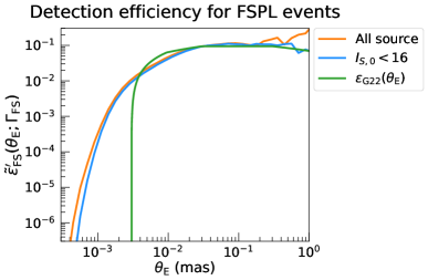
Figure 7: Integrated detection efficiencies for events with $u_{0}<\rho$ and a significant finite source signal as a function of $\theta_{\rm E}$ for all sources (orange line) and giant sources with $I_{\rm s,0}<16$ mag (blue line) from MOA (Koshimoto et al., 2023). and FSPL events from KMTNet (green line) (Gould et al., 2022). $I_{\rm s,0}<16$ mag is the limiting magnitude used by Gould et al. (2022), This is similar to the $\tilde{\epsilon}_{\rm FS}(\theta_{\rm E};\Gamma)$ shown in Figure 8 of K23, except that K23 do not include the $u_{0}<\rho$ condition. These are only for the comparison to Gould et al. (2022) and not used for our analysis.

The MOA sensitivity for giant sources is less than that for all sources at small $\theta_{\rm E}$ because the large $\theta_{*}$ values for giant sources can significantly reduce the peak microlensing magnification. However, the sensitivity curve for KMTNet is very different from that of MOA, with a much sharper cutoff at small $\theta_{\rm E}$. This is partly because they directly cut off their integrated detection efficiency with a cut excluding events with $\theta_{\rm E}<3\,\mu$as. Gould et al. (2022) describe this cut by saying “we complete this function linearly by imposing a threshold at $\theta_{\rm E}=3\,\mu$as, which is supported by the fact that all four FFPs are pressed up close to this limit.” It is difficult to understand they would need a cut like this given the sensitivity calculated for our analysis. Similarly, two of the four FFP events with finite source effects found by OGLE (Mróz et al., 2018, 2019b, 2020b, 2020c) have $\theta_{\rm E}<3\,\mu$as (see Table 1) even though they have source stars with $I_{\rm s,0}<16$. Perhaps the rationale for this cut that requires $\theta_{\rm E}>3\,\mu$as is to make their analysis consistent with their power-law prior assumption of $0.9\lesssim p\lesssim 1.2$. However, if this is the reason for this cut, it would raise the question as to why KMTNet has not been able to find events with $\theta_{\rm E}<3\,\mu$as in contrast to MOA and OGLE who clearly have sensitivity well below this limit with bright sources with $I_{\rm s,0}<16$. It would be helpful to see a full analysis for the KMTNet data set including a complete detection efficiency analysis that includes both the $t_{\rm E}$ and $\theta_{\rm E}$ dependence.

Note that our analysis does not use this integrated detection efficiency that depends only on $\theta_{\rm E}$. This integrated detection efficiency is included only for comparison with the Gould et al. (2022) analysis.

References

- Adams, Anderson & Bloch (2013) Adams, F. C., Anderson, K. R., & Bloch, A. M. 2013, MNRAS, 432, 438
- Agol (2003) Agol, E. 2003, ApJ, 594, 449
- Bennett et al. (2010) Bennett, D. P., Rhie, S. H., Nikolaev, S., et al. 2010, ApJ, 713, 837
- Bennett et al. (2012) Bennett, D. P., Sumi, T., Bond, I. A., et al. 2012, ApJ, 757, 119
- Boss et al. (2003) Boss, A. P., Basri, G., Kumar, S. S., et al. 2003, Brown Dwarfs, 211, 529
- Bozza et al. (2018) Bozza V., Bachelet, E., & Bartolić, F., et al., 2018, MNRAS, 479, 5157
- Bryant et al. (2023) Bryant, E. M., Bayliss, D., & Van Eylen, V. 2023, arXiv:2303.00659. doi:10.48550/arXiv.2303.00659
- Cassan et al. (2012) Cassan, A., Kubas, D., Beaulieu, J. P., et al. 2012, Nature, 481, 167, doi: 10.1038/nature10684
- Coleman, Nelson & Triaud (2023) Coleman G. A. L., Nelson R. P., & Triaud, A. H. M. J. 2023, MNRAS, 522, 4352
- Foreman-Mackey et al. (2014) Foreman-Mackey, D., Hogg, D. W., & Morton, T. D. 2014, ApJ, 795, 64. doi:10.1088/0004-637X/795/1/64
- Gaudi et al. (2008) Gaudi, B. S., Bennett, D. P., Udalski, A., et al. 2008, Science, 319, 927
- Ge et al. (2022) Ge, J., Zhang, H., Zang, W. et al. 2022, arXiv:2206.06693
- Gould et al. (2022) Gould, A. et al. 2022, Journal of the Korean Astronomical Society, 55, 173
- Han & Gould (1996) Han, C. & Gould, A. 1996, ApJ, 467, 540. doi:10.1086/177631
- Hashino et al. (2022) Hashino, K., Kanemura, S., & Takahashi, T. 2022, Physics Letters B, 833, 137261. doi:10.1016/j.physletb.2022.137261
- Hogg et al. (2010) Hogg, D. W., Myers, A. D., & Bovy, J. 2010, ApJ, 725, 2166. doi:10.1088/0004-637X/725/2/2166
- Holtzman et al. (1998) Holtzman, J. A., Watson, A. M., Baum, W. A., et al. 1998, AJ, 115, 1946
- Johnson et al. (2020) Johnson, S. A., Penny, M. & Gaudi, B. S., et al. 2020, AJ, 160, 123
- Hsu, Ford, Ragozzine & Ashby (2019) Hsu, D. C., Ford, E. B., Ragozzine, D.& Ashby, K. 2019, AJ, 158, 109
- Hsu, Ford & Terrien (2020) Hsu, D. C., Ford, E. B., Terrien, R. 2020, MNRAS, 498, 2249
- Jung et al. (2019) Jung, Y. K., Gould, A., & Zang, W., et al. 2019, AJ, 157, 72
- Kim et al. (2021) Kim, H.-W., Hwang, K.-H., Gould, A., et al. 2021, AJ, 162, 15
- Koshimoto et al. (2021a) Koshimoto, N., Baba, J., & Bennett, D. P. 2021a, ApJ, 917, 78. doi:10.3847/1538-4357/ac07a8
- Koshimoto et al. (2021b) Koshimoto, N., Bennett, D. P., Suzuki, D., et al. 2021b, ApJ, 918, L8. doi:10.3847/2041-8213/ac17ec
- Koshimoto et al. (2023) Koshimoto, N., Sumi, T. and Bennett, D. P., et al. 2023, ApJ, submitted (K23)
- Lam et al. (2020) Lam, C. Y., Lu, J. R., Hosek, M. W., et al. 2020, ApJ, 889, 31. doi:10.3847/1538-4357/ab5fd3
- Lin & Ida (1997) Lin, D. N. C. & Ida, S. 1997, ApJ, 477, 781. doi:10.1086/303738
- Maeder (1973) Maeder, A. 1973, A&A, 26, 215
- Malmberg et al. (2011) Malmberg, D., Davies, M. B., & Heggie, D. C. 2011, MNRAS, 411, 859
- Mao & Paczyński (1991) Mao, S., & Paczyński, B. 1991, ApJ, 374, L37
- Metropolis et al. (1953) Metropolis, N., Rosenbluth, A. W., Rosenbluth, M. N., Teller, A. H., & Teller, E. 1953, J. Chem. Phys., 21, 1087
- Mróz et al. (2017) Mróz, P. Udalski A., Skowron, J., et al. 2017, Nature, 548, 183
- Mróz et al. (2018) Mróz, P. Y.-H.Ryu, Skowron, J., et al. 2018, ApJ, 155, 121
- Mróz et al. (2019) Mróz, P. Udalski A., Skowron, J., et al. 2019, ApJS, 244, 29
- Mróz et al. (2019b) Mróz, P. Udalski A., Bennett, D. P. et al. 2019, å, 622, A201
- Mróz et al. (2020a) Mróz, P. Udalski A., Szymański, M., et al. 2020, ApJS, 249, 16
- Mróz et al. (2020b) Mróz, P., Poleski, R. & Gould, A. 2020, ApJ, 903, 11
- Mróz et al. (2020c) Mróz, P., Poleski, R., Han, C. 2020, AJ, 159, 262
- Niikura et al. (2019a) Niikura, H., Takada, M. & Yasuda, N. et al. 2019, Nature Astronomy. 3, 524
- Niikura et al. (2019b) Niikura, H., Takada, M. & Yokoyama, S. et al. 2019, PhRvD. 99, 3503
- Paczyński (1986) Paczyński, B. 1986, ApJ, 304, 1
- Paczyński (1991) Paczyński, B. 1991, ApJ, 371, L63
- Press et al. (1992) Press, W. H., Teukolsky, S. A., Vetterling, W. T., et al. 1992, Cambridge: University Press, —c1992, 2nd ed.
- Rasio & Ford (1996) Rasio, F. A. & Ford, E. B. 1996, Science, 274, 954. doi:10.1126/science.274.5289.954
- Riffeser et al. (2006) Riffeser, A., Fliri, J., Seitz, S., & Bender, R. 2006, ApJS, 163, 225
- Ryu et al. (2021) Ryu, Y-H, Mróz, P., Gould, A. 2021, AJ, 161, 126
- Sumi et al. (2003) Sumi, T. et al., 2003, ApJ, 591, 204
- Sumi et al. (2010) Sumi, T. et al., 2010, ApJ, 710, 1641
- Sumi et al. (2011) Sumi, T. et al., 2011, Nature, 473, 349
- Sumi et al. (2013) Sumi, T. Bennett, D. P. & Bond I. A. et al., 2013, ApJ, 778, 150
- Sumi et al. (2016) Sumi, T., Udalski, A., & Bennett, D. P. et al., 2016, ApJ, 825, 112
- Suzuki et al. (2016) Suzuki, D. Bennett, D. P. & Sumi T. et al., 2016, ApJ, 833, 145
- Udalski et al. (1994) Udalski, A. et al. 1994, Acta Astronomica, 44, 165
- Szymański (2011) Szymański, M., Udalski, A. & Soszyński I. et al. 2011, Acta Astronomica, 61, 83
- Udalski et al. (2018) Udalski,A., Ryu, Y.-H., Sajadian, S., et al. 2018, AcA, 68, 1
- Weidenschilling & Marzari (1996) Weidenschilling, S. J. & Marzari, F. 1996, Nature, 384, 619. doi:10.1038/384619a0
- Zang et al. (2022) Zang, W., Yang, H., Han, C., et al. 2022, MNRAS, 515, 928. doi:10.1093/mnras/stac1883