MELON: NeRF with Unposed Images in SO(3)

Abstract

Neural radiance fields enable novel-view synthesis and scene reconstruction with photorealistic quality from a few images, but require known and accurate camera poses. Conventional pose estimation algorithms fail on smooth or self-similar scenes, while methods performing inverse rendering from unposed views require a rough initialization of the camera orientations. The main difficulty of pose estimation lies in real-life objects being almost invariant under certain transformations, making the photometric distance between rendered views non-convex with respect to the camera parameters. Using an equivalence relation that matches the distribution of local minima in camera space, we reduce this space to its quotient set, in which pose estimation becomes a more convex problem. Using a neural-network to regularize pose estimation, we demonstrate that our method – MELON – can reconstruct a neural radiance field from unposed images with state-of-the-art accuracy while requiring ten times fewer views than adversarial approaches.

1 Introduction

Neural rendering methods have demonstrated wide ranging application from novel-view synthesis [44], to avatar generation for virtual reality  [21], to 3D reconstruction of molecules from microscope images  [33]. Neural radiance fields (NeRFs) [44] represent radiance with a neural field that reproduces the geometric structure and appearance of a scene, allowing the use of gradient descent to reconstruct a set of input images. NeRFs have gained wide acceptance for their robust ability to generate novel-views of a 3D scene, but must be trained with known camera poses, limiting their use to cases where camera pose is known or can be inferred from other methods. Our method seeks to estimate camera pose and radiance field simultaneously, eliminating the requirement of known camera poses.

Classical structure-from-motion algorithms (SfM), such as COLMAP [63], compute the relative camera pose between views by detecting and matching salient points in the scene and minimizing re-projection error. Despite being widely used, SfM commonly fails on scenes containing many view-dependent effects or few textures and edges. Other methods [38, 72, 11] jointly estimate a neural radiance field and camera parameters using gradient descent, but require an approximate initialization of camera parameters, and none work in a $360^{\circ}$ object centered configuration with random initialization. Adversarial approaches [23, 49, 50, 51, 6, 43] jointly train a 3D generator representing the scene, and a discriminator that attempts to differentiate input images from generated images. These methods, however, suffer from large input data requirements, hyper parameter sensitivity, complex training schedules, and high computation times.

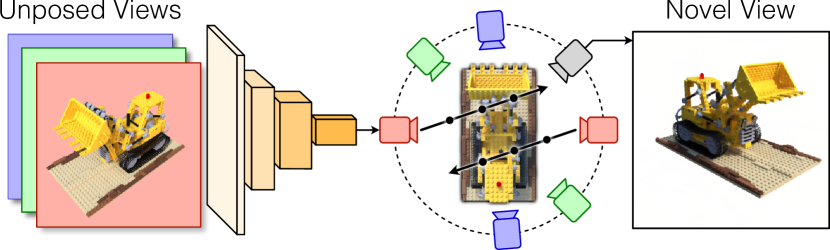
Figure 1: MELON infers a neural radiance field from an object-centered dataset. A dataset-specific encoder maps each image to a predicted pose $R_{i}$. Given an equivalence relation in camera space, we render rays from all the poses in the equivalence class $[R_{i}]$. The modulo loss only penalizes the smallest L2 distance from the ground truth color. At evaluation time, the neural field can be used to generate novel views.

We introduce MELON (Modulo-Equivalent Latent Optimization of NeRF), an encoder-decoder-based method that infers a neural representation of a scene from unposed views (Fig. 1). Our method simultaneously trains a CNN encoder that maps images to camera poses in $\text{SO}(3)$, and a neural radiance field of the scene. MELON does not require CNN pre-training, and is able to infer camera pose in object centered configurations entirely “ab-initio”, i.e. without any pose initialization whatsoever. To cope with the presence of local minima in the low-dimensional latent space $\text{SO}(3)$, we introduce a novel modulo loss that replicates the encoder output following a pre-defined structure. We formalize this replication with an equivalence relation defined in the space of camera parameters, and show this enables the encoder to operate in a quotient set of the camera space. We introduce a one-dimensional toy problem that mimics the challenges posed by 3D inverse rendering to better illustrate our method.

We identify the following contributions:

• We introduce a gradient-descent-based algorithm to train a neural radiance field from entirely unposed images, demonstrating competitive reconstruction metrics on a variety of synthetic and real datasets.

• We show that MELON is robust to noise and can perform pose estimation and novel-view synthesis from as few as six unposed images.

• We introduce 1D and 3D datasets of almost symmetric objects which can be used as challenging examples for pose estimation and inverse rendering.

Our code will be released upon publication.

2 Related Work

Neural Radiance Fields (NeRF)

[44] use classical volume rendering [28] to compute the RGB values $C$ for each pixel $\mathbf{p}$ from samples taken at points $\mathbf{r}$ along a ray of direction $\mathbf{d}$. The ray direction is determined by the camera parameters $R$ and the pixel location. These samples are computed using learned radiance ($\mathbf{c}$) and density ($\sigma$) fields. The volume rendering equation takes the form of an integral along a ray between near and far view boundaries $(t_{n},t_{f})$:

$$C(\mathbf{p}~{};\mathbf{c},\sigma,R)=\int_{t_{n}}^{t_{f}}T(t)\sigma(\mathbf{r}(t))\mathbf{c}(\mathbf{r}(t),\mathbf{d})\mathop{}\!\mathrm{d}t$$ (1)

where the transmittance is given by

$$T(t)=\exp\left(-\int_{t_{n}}^{t}\sigma(\mathbf{r}(s))\mathop{}\!\mathrm{d}s\right).$$ (2)

Neural Radiance Fields have proven capable of high-quality novel view synthesis and have been a recent focus in the research community. They have been extended in many ways including training from noisy HDR images [45], grid-based representations for faster training and inference [68, 46, 70, 59], training with limited or single views [76, 26, 74], decomposition into sub-fields [58, 59], unconstrained images in the wild [42], deformable fields [54, 52, 57], and video [35]. Most of these techniques however assume camera poses to be given, and automatically inferring them during training remains an open research question.

Structure-from-Motion. Reconstruction from unposed images has been a major thrust of research in the structure from motion community for many years [53, 25]. COLMAP [63] is currently the most commonly used method to infer pose when unavailable. Though robustly usable for a number of cases, COLMAP relies on SIFT feature matching and can fail in cases where SIFT features cannot be found, such as scenes with limited edges, corners and texture, or view-dependent effects like reflections, refractions or specular surfaces.

Neural Representations without Poses. Pose estimation of neural scenes can be divided into those which assume a known scene, and those which simultaneously reconstruct a scene along with poses. Of those assuming a known scene, iNeRF [75], further extended by [39], demonstrated that pose could be recovered with stochastic gradient descent and “interest region sampling”, when initialized within $\pm 40^{\circ}$ of ground truth orientation.

NeRF [72] was the first to co-optimize a neural field and 6-DOF camera poses simultaneously. To avoid local minima, the neural field was re-initialized mid-training, and results were only shown for forward-facing scenes. BARF [38] proposed a coarse-to-fine positional encoding annealing strategy [54] and GARF [11] argued that Gaussian activation functions were more robust for pose estimation. SCNeRF [27] extended the parameterization to include camera instrinsics and, like SPARF [69], incorporated multi-view geometric constraints. These methods avoid the need to re-initialize the field and demonstrated results for non forward-facing scenes, but require a rough initialization of the camera poses. SAMURAI [4] simultaneously optimizes several cameras with a novel camera parameterization and tackles non forward-facing scenes but requires poses to be initialized to one of 26 possible directions. NoPe-NeRF [3] introduces additional supervision from an off-the-shelf monocular depth estimation network and novel losses that encourage 3D consistency between the scene and successive frames in a video sequence. All these techniques require initialization within some fixed bound of ground truth pose, or a series of views known to be close in pose to one another.

Approaches like iMAP [67] or NICE-SLAM [81] perform reconstruction from hand-held camera, but requires depth information and ignore view-dependence in the neural field.

Adversarial Approaches [23, 49, 50, 6] jointly supervise a generator containing a differentiable neural field and a discriminator. Such techniques enable the reconstruction of a radiance field while bypassing the pose estimation problem. GNeRF [43] trains on a single scene by supplying image crops to the discriminator, increasing the effective data set size. It co-trains a pose encoder supervised with renderings of the neural scene, which is then used to estimate ground truth image poses. Using a complex training schedule GNeRF, is able to reconstruct a single scene from completely unposed images. VMRF [77] refined this work by using a pre-trained feature detector, differentiable unbalanced optimal transport solver and relative pose predictor to provide extra supervision achieving better reconstruction and pose estimation than GNeRF.

Although such techniques enable the reconstruction of a photo-realistic 3D field from unposed images, they require large datasets for training the discriminator, complex training schedules, and suffer the inherent instabilities and hyper-parameter sensitivities of GANs.

Supervised Pose Regression methods approach the pose estimation (or “camera calibration”) problem as a regression problem, where a mapping from image space to pose space needs to be approximated [24, 37, 30, 29, 41, 66, 36, 40] and [62] analyzed the limits of CNN-based methods. Focusing on the degenerate case of symmetric objects, Implicit-PDF [47] showed that an image can be mapped to a multimodal posterior distributions stored in a coordinate-based representation and RelPose [78] introduced an energy-based approach to estimate joint distribution over relative viewpoints in $\text{SO}(3)$. SparsePose [65] trains a coarse pose regression model on a large dataset and refines camera poses in $\text{SE}(3)$ in an auto-regressive manner. However, these approaches require training over a large data set with known poses and do not provide a neural field of the scene.

Previous works proposed ways to build rotation-equivariant networks [14, 15, 1, 20, 9, 16, 17, 48]. Such symmetry-aware networks showed improved generalization properties for processing point clouds or spherical images but do not ensure $\text{SO}(3)$-equivariance for pose estimation since no group action for the group $\text{SO}(3)$ can be defined on the set of 2D images [32].

Unsupervised Approaches use an encoder–decoder architecture mapping the image space to an $\text{SO}(3)$-valued latent space and mapping this space back to the image space with a group-equivariant generative model [18]. Spatial-VAE [2] demonstrated translation and in-plane rotation estimation for 2D images using a neural-based 2D generative model in the decoder, while TARGET-VAE [48] proposed to use a translation and in-plane rotation equivariant encoder. SaNeRF [10] runs classical COLMAP SIFT feature detection and mapping, but regresses relative poses from a triplet of images fed to a CNN. As it uses SIFT feature matching, this method is not suitable for objects containing large texture-less regions or repeated structures.

Approaches from the Cryo-Electron Microscopy (Cryo-EM) community [34, 33] recently showed the possibility of using an auto-encoding approach to reconstruct a 3D neural field in Fourier domain [80, 64] from unposed 2D projections. These methods do not require any initialization for the poses and have been shown to work on datasets with high levels of noise. The image formation model in cryo-EM is orthographic and does not involve opacity, allowing faster computation with the Fourier Slice Theorem. Building on these approaches, our method copes with a more complex rendering equation that incorporates perspective and opacity.

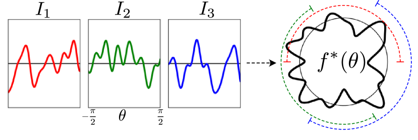
Figure 2: 1D inverse rendering. We are given a set of crops $I_{i}$ from an unknown function $f^{*}(\theta)$ mapping $\text{SO}(2)$ to $\mathbb{R}$. Each crop has size $\pi$ and is centered around an unknown angle $\theta_{i}^{*}$. The goal is to recover the function (and the angles) given the crops.

3 Methods

We are given a set of input images $\{I_{i}\}_{i=1\ldots n}$ which we assume to be renderings of an unknown density $\sigma^{*}$ and view-dependent radiance $\mathbf{c}^{*}$ field from unknown cameras $\{R_{i}^{*}\}_{i=1,\ldots,n}$, following (1):

$$\forall i,\forall\mathbf{p}\in\mathcal{P},\quad I_{i}(\mathbf{p})=C(\mathbf{p}~{};f^{*},R_{i}^{*})$$ (3)

where $\mathcal{P}$ is a discrete set of pixel coordinates and $f^{*}=(\mathbf{c}^{*},\sigma^{*})$. We assume that all cameras have known intrinsics and point towards the origin of the scene from a known distance. Each camera orientation $R_{i}\in\text{SO}(3)$ can therefore be described with three numbers: azimuth $\theta\in\text{SO}(2)$, elevation $\phi\in[-\pi/2,\pi/2]$ and roll $\alpha\in\text{SO}(2)$. We use the symbol $\sim$ to represent an element of $\text{SO}(3)$ in this coordinate system. We define (external) additive and multiplicative operations such that, for $\theta_{0}\in\text{SO}(2)$, $\lambda\in\mathbb{R}$ and $R\sim(\theta,\phi,\alpha)$,

$$\theta_{0}+R\sim(\theta_{0}+\theta,\phi,\alpha)\quad;\quad\lambda R\sim(\lambda\theta,\phi,\alpha).$$ (4)

We use a neural radiance field parameterized by $\psi$ to represent the predicted function $f_{\psi}=(\mathbf{c}_{\psi},\sigma_{\psi})$. The goal of 3D inverse rendering with unknown poses is to approximate $f^{*}$ with $f_{\psi}$ and $R_{i}^{*}$ with $R_{i}$, up to a global rotation. While $\psi$ is shared, each image is associated with a unique $R_{i}$, called a latent variable living in the latent space $\text{SO}(3)$. The low dimensionality of this space induces the presence of local minima [5, 13] and makes pose estimation difficult to solve by gradient descent.

3.1 One-dimensional Toy Problem

We propose a simpler 1D version of the above problem to aid us in understanding the challenges existing in 3D space (Fig. 2). Assume we are given $n$ crops $\{I_{i}\}_{i=1,\ldots,n}$ of width $\pi$ of an unknown one-dimensional function $f^{*}$ mapping $\text{SO}(2)$ to $\mathbb{R}$. Each crop $I_{i}$ is centered around an unknown angle $\theta_{i}^{*}$:

$$\forall i,\forall\theta\in S,\quad I_{i}(\theta)=C(\theta~{};f^{*},\theta_{i}^{*})=f^{*}(\theta_{i}^{*}+\theta)$$ (5)

where $S=[-\pi/2,\pi/2]\subset\text{SO}(2)$. Our objective is to recover the function $f^{*}$ given the crops $I_{i}$, without knowing the set of angles $\{\theta_{i}^{*}\}$.

The objective of 1D inverse rendering with unknown angles is to approximate $f^{*}$ with a coordinate-based neural network $f_{\psi}$ and $\theta_{i}^{*}$ with $\theta_{i}$, up to a global rotation. In this case, the latent variables are the angles $\theta_{i}$ belonging to the latent space $\text{SO}(2)$.

3.2 Amortized Inference of Latent Variables

In both problems, a set of latent variables $z_{i}$ must be estimated ($R_{i}$ in 3D, $\theta_{i}$ in 1D) jointly with a parameter $\psi$. Instead of minimizing $\norm\big{C(.~{};f_{\psi},z_{i})-I_{i}(.)}_{2}^{2}$ over each $z_{i}$ independently, we aim to find an encoder $h$ mapping observations $I_{i}$ (images or crops) to their associated latent variables $z_{i}^{*}$. The encoder is parameterized by a neural network with weights $\xi$ (see details on the architecture in the supplements). The objective function of our optimization is therefore

$$\mathcal{L}(\psi,\xi)=\sum_{i=1}^{n}\norm\big{C(.~{};f_{\psi},h_{\xi}(I_{i}))-I_{i}(.)}_{2}^{2},$$ (6)

where $\|.\|_{2}$ is the L2 norm on the plane $\mathcal{P}$ or segment $S$. We say that the inference of the latent variables is amortized over the size of the dataset, meaning that the estimation of the latent variables for the dataset is seen as a unique inference problem instead of $n$ independent problems. In particular, if $h$ is accurate on a given observation $I_{i}$, it will likely be accurate on similar observations provided that it is likely to be smooth in observation space.

3.3 Self-Similarity Map

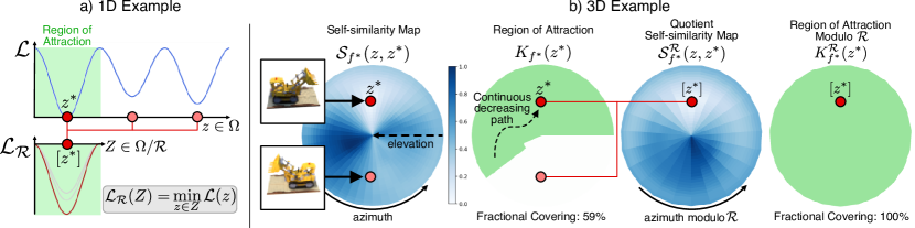
Figure 3: (a) One-dimensional quasi-periodic loss $\mathcal{L}$ defined on $\Omega=\text{SO}(2)$, minimized by $z^{*}$, and modulo loss $\mathcal{L}_{\mathcal{R}}$ defined on $\Omega/\mathcal{R}$. The region of attraction is the set of $z$’s that can be connected to $z^{*}$ with a path where $\mathcal{L}$ always decreases. In this example, the modulo loss is convex for $\mathcal{R}=\mathcal{R}_{3}$. (b) Self-similarity map and region of attraction on the Lego scene for all azimuths and elevations, fixed in-plane roll and a fixed reference camera pose $z^{*}$. The self-similarity map shows the photometric distance to the reference image with respect to the rendering pose $z\in\Omega$. The region of attraction covers all the quotient set $\Omega/\mathcal{R}$ when $\mathcal{R}=\mathcal{R}_{2}$. See supplements for the self-similarity-map of the Lego scene with a fixed elevation and a variable reference $z^{*}$.

Let $\Omega$ be the latent space ($\text{SO}(2)$ or $\text{SO}(3)$) and $C$ our rendering model. In both cases, we can provide $\Omega$ with an internal binary operation $\cdot$ and see $(\Omega,\cdot)$ as a group. In order to focus our analysis on the pose estimation problem, we will make the simplifying assumption that $f_{\psi}$ approximates $f^{*}$, up to a global alignment $z_{0}\in\Omega$, i.e.

$$\forall z\in\Omega,\quad C(.~{};f^{*},z_{0}\cdot z)=C(.~{};f_{\psi},z).$$ (7)

We define the self-similarity map of $f^{*}$ as

$$\mathcal{S}_{f^{*}}:\begin{cases}\Omega^{2}&\to\mathbb{R}_{+}\\ (z,z^{*})&\mapsto\norm\big{C(.~{};f^{*},z)-C(.~{};f^{*},z^{*})}_{2}^{2}\end{cases},$$ (8)

Given (7), the loss (6) can be re-written

$$\mathcal{L}(\xi)=\sum_{i=1}^{n}\mathcal{S}_{f^{*}}(z_{0}\cdot h_{\xi}(I_{i}),z^{*}_{i}).$$ (9)

By the chain rule, the computation of $\nabla_{\xi}\mathcal{L}$ involves the gradients of $\mathcal{S}_{f^{*}}(.,z^{*}_{i})$. As the loss is minimized by gradient descent, the model can converge to the optimal solution only if it does not need to cross “bariers” in the energy landscape to reach a global minimum, i.e. if there exists a continuous path in $\Omega$ between the initial value $z_{0}\cdot h_{\xi}(I_{i})$ and $z^{*}_{i}$ where $\mathcal{S}_{f^{*}}(.,z^{*}_{i})$ is strictly decreasing. For $z^{*}\in\Omega$, we write $K_{f^{*}}(z^{*})$ the set of initial values satisfying the above condition and call it the region of attraction of $z^{*}$ for $f^{*}$. The difficulty of the pose estimation problem with random initialization can therefore be related to the fractional size of the regions of attraction of $f^{*}$:

$$0\leq D(f^{*})=\mathbb{E}_{z^{*}\sim p^{*},z\sim p}[z\in K_{f^{*}}(z^{*})]\leq 1,$$ (10)

where $p=p^{*}$ is the uniform distribution over the latent space $\Omega$. The closer this value to $1$, the easier pose estimation will be.

3.4 Modulo Loss: From Latent to Quotient Space

Our core idea is to let the encoder work in a smaller space than the latent space, namely in the quotient set of the latent space for some equivalence relation. Given an equivalence relation $\mathcal{R}$ (reflexive, transitive and symmetric), we map each latent $h_{\xi}(I_{i})$ predicted by the encoder to its equivalence class

$$[h_{\xi}(I_{i})]_{\mathcal{R}}=\{z~{}|~{}z\mathcal{R}h_{\xi}(I_{i})\}.$$ (11)

All the latents belonging to this class are passed to the rendering model to generate a set of synthetic observations

$$\mathcal{C}_{i}^{\mathcal{R}}(\psi,\xi)=\{C(.~{};f_{\psi},z),z\in[h_{\xi}(I_{i})]_{\mathcal{R}}\}.$$ (12)

The L2 distances are computed between the ground truth observation and all the generated views. The function we minimize, called the modulo loss, is defined as

$$\mathcal{L}_{\mathcal{R}}(\psi,\xi)=\sum_{i=1}^{n}\text{min}\{\|C-I_{i}\|_{2}^{2},C\in\mathcal{C}_{i}^{\mathcal{R}}(\psi,\xi)\}.$$ (13)

and is a lower bound of (6) due to the reflexivity of $\mathcal{R}$. Given our simplifying assumption (7), the modulo loss can be re-written

$$\mathcal{L}_{\mathcal{R}}(\xi)=\sum_{i=1}^{n}\mathcal{S}_{f^{*}}^{\mathcal{R}}([z_{0}\cdot h_{\xi}(I_{i})]_{\mathcal{R}},z^{*}_{i})\leq\mathcal{L}(\xi)$$ (14)

where the quotient self-similarity map $\mathcal{S}_{f^{*}}^{\mathcal{R}}$ is defined by

$$\mathcal{S}_{f^{*}}^{\mathcal{R}}:\begin{cases}\Omega/\mathcal{R}\times\Omega&\to\mathbb{R}_{+}\\ (Z,z^{*})&\mapsto\text{min}\{\mathcal{S}_{f^{*}}(z^{\prime},z^{*}),z^{\prime}\in Z\}\end{cases}.$$ (15)

This loss is minimized when $z_{i}^{*}\in[z_{0}\cdot h_{\xi}(I_{i})]_{\mathcal{R}}$ for all $i$. Given an optimal encoder, $h_{\xi^{*}}(I_{i})$ is an estimate of $z_{i}$ modulo $\mathcal{R}$ and the true estimate is given by

$$z_{i}=\text{argmin}\{\|C(.~{};f_{\psi},z)-I_{i}(.)\|_{2}^{2},z\in[h_{\xi^{*}}(I_{i})]\}.$$ (16)

As previously, we introduce $K^{\mathcal{R}}_{f^{*}}(z^{*})$, the region of attraction of $z^{*}$ for $f^{*}$ modulo $\mathcal{R}$, as the set of $Z\in\Omega/\mathcal{R}$ such that there exists a continuous path in $\Omega/\mathcal{R}$ between $Z$ and $[z^{*}]_{\mathcal{R}}$ where $\mathcal{S}_{f^{*}}^{\mathcal{R}}(.,z^{*})$ is strictly decreasing. The difficulty of the pose estimation problem in the quotient space is inversely correlated to the expected fractional covering of $K^{\mathcal{R}}_{f^{*}}(z^{*})$,

$$0\leq D_{\mathcal{R}}(f^{*})=\mathbb{E}_{z^{*}\sim p^{*},z\sim p}[z\in K^{\mathcal{R}}_{f^{*}}(z^{*})]\leq 1,$$ (17)

where $p$ is the uniform distribution over $\Omega/\mathcal{R}$ and $p^{*}$ the uniform distribution over $\Omega$. Fig. 3 illustrates the notions of modulo loss, self-similarity map and region of attraction (for a fixed reference $z^{*}$) in 1D and 3D.

Although $K^{\mathcal{R}}_{f^{*}}$ cannot be computed when $f^{*}$ is unknown, the relation $\mathcal{R}$ can be chosen in a way that matches the general structure of $\mathcal{S}_{f^{*}}$. For both inverse rendering problems, we introduce an equivalence relation $\mathcal{R}_{N}$, parameterized by $N\in\mathbb{N}^{*}$ and defined by

$$z\mathcal{R}_{N}z^{\prime}\quad\text{iff}\quad\exists k\in\mathbb{Z},z=\frac{2k\pi}{N}+z^{\prime}.$$ (18)

$N$ corresponds to the number of distinct elements in $[z]$ and will be called the “replication order”. In 3D, $\mathcal{R}_{N}$ induces a replication of the cameras along the azimuthal dimension and is well-chosen for natural objects, which tend to be pseudo-symmetric by rotation around the vertical axis. For all $N\in\mathbb{N}^{*}$, a natural homoemorphism $F:\Omega\to\Omega/\mathcal{R}$ is defined by $F(z)=[z/N]$. The quotient space $\Omega/\mathcal{R}$ can be seen as “$N$ times smaller” than $\Omega$.

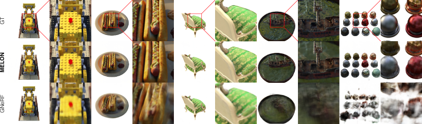
Figure 4: Qualitative comparison between MELON and GNeRF for novel view synthesis (test set) on “NeRF-Synthetic” scenes.

4 Results

4.1 Datasets

		Pose Estimation				Novel View Synthesis
		Rotation (∘) $\downarrow$				PSNR $\uparrow$			SSIM $\uparrow$			LPIPS $\downarrow$
Scene	$N$	COLMAP		GNeRF	MELON	GNeRF	MELON	NeRF	GNeRF	MELON	NeRF	GNeRF	MELON	NeRF
Lego	2	0.229	(100)	2.006	0.061	24.62	29.07	30.44	0.8756	0.9430	0.9526	0.1373	0.0687	0.0591
Hotdog	2	0.328	(91)	9.518	0.853	26.23	31.58	35.97	0.9304	0.9608	0.9782	0.1284	0.0669	0.0384
Chair	2	9.711	(100)	1.181	0.124	29.45	29.72	32.45	0.9346	0.9491	0.9673	0.0988	0.0708	0.0558
Drums	2	0.467	(21)	1.602	0.048	22.58	24.38	24.43	0.8893	0.9091	0.9120	0.1577	0.1169	0.1095
Mic	2	0.860	(15)	1.535	0.057	28.32	28.66	31.83	0.9527	0.9582	0.9705	0.0765	0.0620	0.0465
Ship	2	0.292	(10)	27.84	0.113	15.72	26.87	27.71	0.7704	0.8390	0.8553	0.4068	0.1847	0.1719
Materials	4	1.053	(17)	38.43	5.607	13.13	23.43	29.57	0.7538	0.8914	0.9540	0.4031	0.1620	0.0725
Ficus	2	fails		45.88	8.977	17.85	22.85	25.63	0.8493	0.9132	0.9366	0.2594	0.1321	0.0892

Table 1: Pose estimation (training set) and novel view synthesis (test set) quality for competing methods on “NeRF-Synthetic” scenes. $N$ is the replication order used with MELON. “NeRF” is our implementation with ground truth cameras for baseline reference. GNeRF and MELON predict the elevation only within the respective range of the scene (see supp.) We report the best of five runs for GNeRF and MELON. COLMAP column left: mean error on solved poses, right: number of solved poses. We penalize unsolved COLMAP poses with the mean of a random guess when bolding for fair comparison to GNeRF and MELON, which always predict pose.

1D Dataset We generate random functions $f^{*}$ that map $\text{SO}(2)$ to $\mathbb{R}$ by randomly drawing their $512$ first Fourier coefficients $c_{k}$ following a centered Gaussian distribution. The expected magnitudes of these Fourier coefficients is $\exp(-|k|/5)$ and we make the functions quasi-periodic by setting $c_{\pm 2}=100$. We generate ten one-dimensional functions containing $256$ crops of $65$ uniformly spaced samples of $f^{*}$. We show an example of ground truth function and its self-similarity map in the supplements.

RGB-MELON We build a pathological dataset containing centered views of 3D spheres on which we map quasi-symmetric textures. We use spherical harmonics to generate red-green textures that are invariant by translation of $2\pi/K$ along the azimuthal direction, with a tunable symmetry order parameter $K\in\{1,2,3,4\}$. In order to break the perfect symmetry of these scenes, we add three red/green/blue squares along the azimuthal direction. We generate $116$ views from a fixed and known distance, with all the cameras located in the equator plane. We hold out $16$ test images in each dataset. Sample views of these datasets are provided in the supplements.

“NeRF-Synthetic” Dataset We use the eight object-centric scenes provided by [44], which consist of $300$ rendered images (downscaled to $400\times 400$ pixels) and ground truth camera poses for each scene. All the methods evaluated on these datasets assume the object-to-camera distance and the “up” direction to be known (fixed roll $\alpha$). We hold out the $200$ “test” views, using them only for evaluation.

Real-World Datasets We evaluate our method using three real-world scenes: the Gold Cape [56] and the Ethiopian Head [55] from the British Museum’s photogrammetry dataset, and a Toytruck from the Common Object in 3D (CO3D) dataset [61]. These scenes are approximately object-centered and were recorded with fixed illumination conditions. We consider the published camera poses as ground truth. We use ground truth masks to remove the background before computing the photometric loss.

4.2 1D Inverse Rendering

In our 1D study we map crops to predicted angles with an encoder, trivially ”render” with the identity following (5), use the modulo loss and reconstruct the function $f_{\psi}$ with a neural network (positional encoding [44] and four fully-connected layers of size 64 with ReLU activation functions). We perform an ablation study and separately (1) replace the neural representation $f_{\psi}$ with an explicit representation, (2) replace the modulo loss with an L2 loss and (3) replace the encoder with a set of independently optimized angles. We use the Adam optimizer [31] with a learning rate of $10^{-4}$ and $256$ crops per batch. We align the predicted angles (as defined by (16)) and the predicted function to the ground truth before computing mean square errors. As shown in Fig. 5, the neural representation, the modulo loss and the encoder are all necessary for the method to work, in this order of importance. We hypothesize that explicit grids are not well-suited for this task because they do not have any inductive bias encouraging smoothness. Since the derivative of the loss w.r.t. $\theta_{i}$ involves $f_{\psi}^{\prime}$, gradient-descent gets stuck at an early stage (visual reconstructions in the supplements). The modulo loss mods out the latent space, making it more convex. The encoder leverages the fact that similar images should be mapped to similar poses.

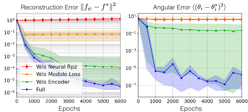
Figure 5: Angular and reconstruction error for the 1D datasets. We indicate the mean, min and max errors obtained throughout $10$ experiments. The explicit representation gets stuck at an early stage. The modulo loss helps the model avoiding local minima and the encoder regularizes the angular prediction.

4.3 NeRF with Unposed Images

Using the “NeRF-Synthetic” dataset, we compare MELON to COLMAP [63] and GNeRF [43] for pose estimation and novel view synthesis. In Table 1, we quantify the accuracy of pose estimation by reporting the mean angular error of the predicted view directions on the training set. We evaluate novel view synthesis quality by computing the Peak Signal Noise Ratio (PSNR), Structural Similarity Index Measure (SSIM) [71] and Learned Perceptual Image Patch Similarity (LPIPS) [79] against all 200 test views. The pose accuracy is reported after applying a global alignment matrix minimizing the mean angular error over $\text{SO}(3)$. A qualitative comparison is shown on Fig. 4. MELON outperforms GNeRF on novel view synthesis, thanks to more accurate estimation of the camera poses. COLMAP fails on scenes where it does not find enough corresponding points (“ficus”) while a small number of outliers significantly increases the mean angular error on “chair”. For fair comparison to GNeRF and MELON, we penalize COLMAP’s unsolved poses with a random guess (see corrected pose accuracy in the supplements).

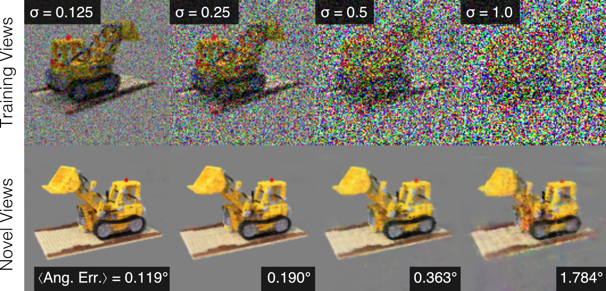
Figure 6: Novel view synthesis from noisy unposed images ($128\times 128$). Mean angular error on the training set indicated in bottom right corners.

4.4 Noise and Number of Views

We illustrate the sensitivity of MELON to noise in Fig. 6. We add white Gaussian noise of variance $\sigma^{2}$ to the training images of the “lego” dataset. For this experiment, we encourage view-consistency using a view-independent neural field. MELON accurately estimates the poses on the training set and generates noise-free novel views. In this context, our method can be seen as a “3D-consistent” unposed image denoiser. A comparison to COLMAP is provided in the supplements.

Unlike adversarial approaches, MELON does not need to train a model to discriminate real from synthetic images, and can therefore perform ab initio inverse rendering with datasets containing few images. We artificially reduce the size of the training set in the “lego” scene and report the results of MELON with a replication order $N=2$ in Table 2. We compare our method to the adversarial approach GNeRF, and to COLMAP. Novel views are shown in the supplements.

COLMAP does not find enough corresponding points when given 16 or less views. In comparison, MELON accurately estimates the poses from only six views while GNeRF’s accuracy significantly degrades when decreasing the number of given views. We hypothesize that supervising the field with slightly wrong cameras at an early stage of training can act as a regularizer and could explain why MELON sometimes gets a marginally higher PSNR than NeRF with ground truth poses.

	Rotation (∘) $\downarrow$				PSNR $\uparrow$
# Views	COLMAP		GNeRF	MELON	GNeRF	MELON	NeRF
4	fails		45.8	1.21	12.59	12.83	18.47
6	fails		35.4	0.509	13.20	18.95	19.75
8	fails		20.0	0.517	14.13	22.57	24.08
12	fails		17.9	0.148	15.02	26.40	26.29
16	fails		11.7	0.135	16.79	27.33	27.20
32	41.2	(20)	12.3	0.122	18.43	29.01	29.07
64	35.3	(64)	4.77	0.101	23.74	30.80	30.31
100	7.66	(100)	0.901	0.095	29.24	31.15	30.72

Table 2: Ab-initio reconstruction with a variable number of views on the “lego” scene (128$\times$128). “NeRF” is our implementation with ground truth cameras. We report the best of three runs for GNeRF and MELON. COLMAP numbers reported as in Table 1.

4.5 Replication Order

MELON

COLMAP

$N=1$ (23 ms/it.)

$N=2$ (34 ms/it.)

$N=3$ (43 ms/it.)

$N=4$ (52 ms/it.)

Sym. Order

$D(f^{*})$

PSNR

Rot. (∘)

$D_{\mathcal{R}}(f^{*})$

PSNR

Rot. (∘)

$D_{\mathcal{R}}(f^{*})$

PSNR

Rot. (∘)

$D_{\mathcal{R}}(f^{*})$

PSNR

Rot. (∘)

Rot. (∘)

1

0.65

36$\pm$1

2.7$\pm$0.5

0.83

36$\pm$1

2.6$\pm$0.5

0.86

37$\pm$1

2.5$\pm$0.5

1.00

37$\pm$1

2.5$\pm$0.5

fails

2

0.52

25$\pm$2

70$\pm$5

0.98

38.6$\pm$0.5

0.7$\pm$0.1

0.55

19$\pm$1

70$\pm$5

1.00

38.7$\pm$0.5

0.7$\pm$0.1

fails

3

0.28

16$\pm$1

72$\pm$5

0.40

21$\pm$2

40$\pm$5

0.65

39.5$\pm$0.5

0.6$\pm$0.1

0.57

29$\pm$5

25$\pm$11

fails

4

0.26

22$\pm$1

75$\pm$5

0.54

26$\pm$1

47$\pm$5

0.35

19$\pm$1

70$\pm$5

1.00

35$\pm$1

3.0$\pm$0.5

fails

Table 3: The fractional size of the regions of attractions $D_{\mathcal{R}}(f^{*})$ gets closer to $1$ when the replication order $N$ is a multiple of the symmetry order $K$ of the sphere. We report the accuracy of novel view synthesis and pose estimation (mean $\pm$ std. over 5 experiments). COLMAP fails due to the repeating patterns in the synthesized textures. Red cells indicate when the mean angular error is above $20^{\circ}$. The compute time of one gradient-step increases linearly with $N$.

We run MELON with a replication order $N\in\{1,2,3,4\}$ to reconstruct the RGB-MELON scenes. In Table 3, we report, for each value of $N$ and each symmetry order $K$, the fractional size $D_{\mathcal{R}}(f^{*})$ of the regions of attraction for $\mathcal{R}=\mathcal{R}_{N}$. This number is closer to $1$ when the replication order “matches” the symmetry order of the dataset, i.e. when $N$ is a multiple of $K$.

We report the quality of novel view synthesis on the test set and pose estimation on the training set. COLMAP fails at estimating the poses due to the presence of repeating patterns and the absence of sharp corners. In comparison, our method converges when the replication order matches the symmetries of the texture. As $N$ increases, our method can cope with a broader range of datasets at the cost of more computation.

4.6 Towards NeRF in the Wild

MELON assumes that all the cameras point towards the center of the scene from a known distance. In a real capture setup, the object-to-camera distance, $r$, is unknown and the cameras do not all point towards a unique point. We parameterize each camera with a camera-to-world rotation matrix $R_{i}\in\text{SO}(3)$ and a three-dimensional vector $T_{i}\in\mathbb{R}^{3}$ that specifies the location of the origin in the camera frame. This vector is constant and equal to $(0,0,r)$ in an ideal object-centered setup.

In Fig. 7, we compare our results to those obtained with GNeRF [43] and SAMURAI [4], for the estimation of the rotation matrix $R_{i}$ only. For all methods, we use the published values for $T_{i}$ and parameterize the elevations in $[0^{\circ},90^{\circ}]$. Since SAMURAI requires the user to manually initialize the camera view directions to one of 26 possible directions, we show the results obtained with a fixed initialization at the North pole for fair comparison. Quantitative results and additional comparison to a manual initialization of SAMURAI are shown in the supplements.

When both the object-to-camera distances and the in-plane camera translations are unknown, the latent space becomes $\text{SE}(3)$ and contains twice as many degrees of freedom as $\text{SO}(3)$. Although it can accurately estimate the rotation matrix $R_{i}$, we show in Fig. 8 that MELON fails at jointly inferring $R_{i}$ and $T_{i}$. In this setup, SAMURAI is the only effective reconstruction method but requires a rough initialization of the camera view directions (see supplements).

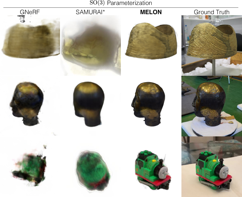
Figure 7: Ab initio reconstruction on real datasets. All the methods use ground truth values for the object-to-camera distances and in-plane camera translations. SAMURAI* uses a fixed initialization of the poses at the North pole.

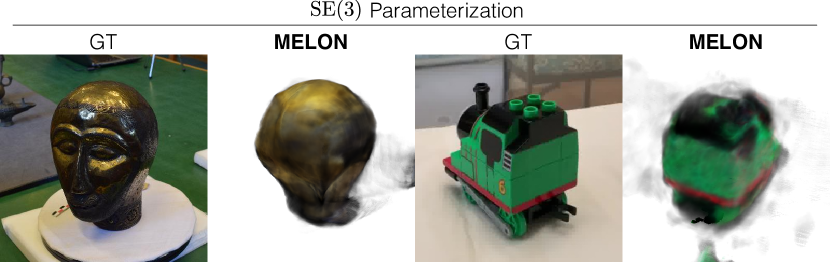
Figure 8: Limitation: MELON fails when the object-to-camera distance and in-plane camera translations are unknown.

5 Discussion

MELON solves the problem of inverse rendering from unposed images using amortized inference and a novel loss function. Using an equivalence relation that matches the distribution of local minima in a given object’s self-similarity map, the modulo loss reduces the camera space to a smaller space (its quotient set), in which gradient descent is more likely to converge. We demonstrated that MELON could perform inverse rendering on a variety of synthetic and real unposed datasets with state-of-the-art accuracy and that MELON could cope with small or noisy datasets.

Characterizing the full loss landscape of 3D inverse rendering with unknown poses remains an open research question. Our theoretical analysis focused on the pose estimation problem only, making the assumption that the reconstructed function $f$ was close to $f^{*}$, up to a global alignment. Although the loss (6) simplified to (9), no inequality generally holds between the two. The full inverse rendering problem contains many more unknown parameters and ambiguities than pose estimation alone. Furthermore, the assumption of a perfectly object-centered setup is too restrictive for reconstructing real world datasets and the prediction of camera extrinsics in $\text{SE}(3)$ remains an open challenge.

We demonstrated the possibility of optimizing a neural radiance field from unposed images. However, other volumetric representations are conceivable, such as tensorial products [7, 8] hash tables [46], or explicit representations [19]. Exploring the strengths of other encodings within the context of our method is a promising future direction.

As real objects often contain rotational symmetries around the vertical axis, we focused on the use of equivalence classes that keep the elevation and roll of the cameras fixed. An interesting extension of this work could be to broaden the scope of equivalence relations used to mod out the latent space $\text{SO}(3)$.

MELON: NeRF with Unposed Images in SO(3)
Supplementary Material

Appendix A Datasets

A.1 1D Dataset

Fig. S1 shows an example of a ground truth 1D function $f^{*}$, its self-similarity maps and its regions of attraction. We show visual results for the ablation study of Fig. 5. Details on the generation process are given in the main paper (4.1). A jupyter notebook for generating these datasets and running our experiments will be provided in an open source repository.

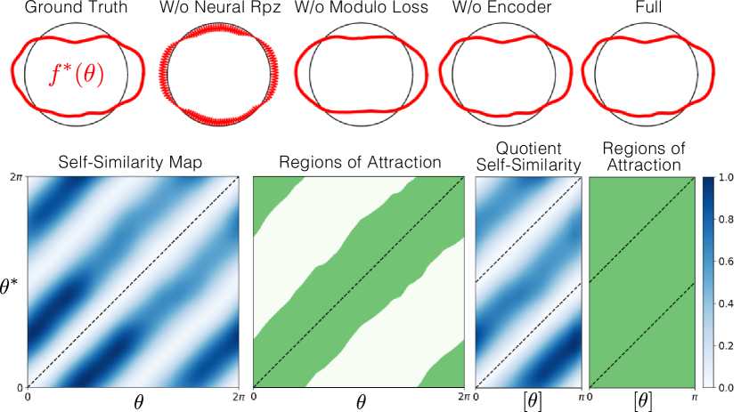
Figure S1: (Top) Example of ground truth function $f^{*}$ and visual results for the ablation study (Fig. 5). (Bottom) Self-similarity maps and regions of attraction. The self-similarity map shows local minima on the line $\theta^{*}=\theta+\pi$. With the equivalence relation $\mathcal{R}=\mathcal{R}_{2}$, the regions of attraction cover the entire quotient set $\Omega/\mathcal{R}$.

A.2 3D Datasets

Table S1 summarizes the properties of the datasets used for 3D inverse rendering. Fig. S2 shows sample views of the RGB-MELON datasets. These datasets and the script for generating them in Blender [12] will be provided upon publication.

Dataset	Synth.	Res.	Train	Test	Roll $=0$	Elev. Range	$N$	Encoder Res.
RGB-M	Yes	128	100	16	Yes	$\{0^{\circ}\}$	1-4	$64\times 64$
Lego [44]	Yes	128-400	2-100	200	Yes	$[0^{\circ},90^{\circ}]$	2	$32\times 32$
Hotdog [44]	Yes	400	100	200	Yes	$[0^{\circ},90^{\circ}]$	2	$128\times 128$
Chair [44]	Yes	400	100	200	Yes	$[0^{\circ},90^{\circ}]$	2	$128\times 128$
Drums [44]	Yes	400	100	200	Yes	$[0^{\circ},90^{\circ}]$	2	$32\times 32$
Mic [44]	Yes	400	100	200	Yes	$[0^{\circ},90^{\circ}]$	2	$32\times 32$
Ship [44]	Yes	400	100	200	Yes	$[0^{\circ},90^{\circ}]$	2	$64\times 64$
Materials [44]	Yes	400	100	200	Yes	$[-90^{\circ},90^{\circ}]$	4	$64\times 64$
Ficus [44]	Yes	400	100	200	Yes	$[-90^{\circ},90^{\circ}]$	2	$128\times 128$
Cape [56]	No	400	99	2	No	$[0^{\circ},90^{\circ}]$	2	$64\times 64$
Head [55]	No	400	64	2	No	$[0^{\circ},90^{\circ}]$	4	$64\times 64$
Toytruck [60]	No	400	84	2	No	$[0^{\circ},90^{\circ}]$	2	$64\times 64$

Table S1: Summary of the 3D datasets. “Synth.” indicates if a scene is synthetic (Yes) or real (No). RGB-M $=$ RGB-MELON. “Train” and “Test” indicate the number of images in the respective splits. $N$ is the replication order used with MELON. For each dataset, we indicate the resolution given at the input of the encoder.

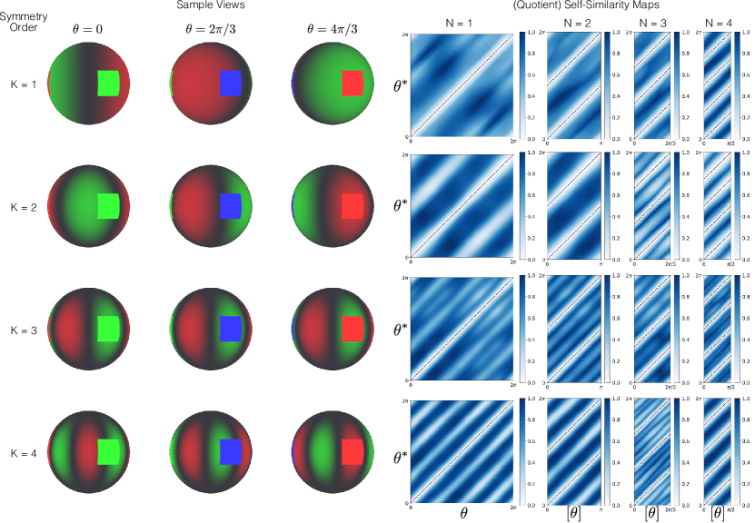
Figure S2: Sample views from the RGB-MELON datasets. The red–green texture is symmetric along the azimuthal direction. In order to make the pose estimation problem well-posed, the symmetry is broken by three red/green/blue squares. All the views are taken from the equator plane. The self-similarity maps and quotient self-similarity maps are plotted on the right for various replication orders $N$.

Appendix B Baselines

B.1 COLMAP

We ran COLMAP with the default configuration for performance evaluations. To ensure fair comparison, we swept parameters, running with different patch window radii (window_radius) of 5, 3, 7, 9, 11, and different filtering thresholds of photometric consistency cost (filter_min_ncc) of 0.1, 0.01, 0.2, 0.5, and 1.0. We tested all combinations of each.

COLMAP fails when it can not find enough corresponding points between frames. When it finds enough points, it does not always solve all the poses. We report the mean angular error over solved poses in the main text. For fair comparison to MELON and GNeRF, which always predict pose, we also compute a mean over all poses where the error of an unsolved pose is counted as a random guess (i.e. $73^{\circ}$ when the elevation range is $[0^{\circ},90^{\circ}]$ and $90^{\circ}$ when it is $[-90^{\circ},90^{\circ}]$). Results are reported in Table S2.

In general, we note that the high mean angular error of COLMAP is due to large errors on few images. The distribution of angular errors (Fig. S3) shows a large discrepancy between the median and the mean.

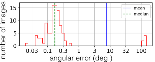
Figure S3: Histogram of angular errors obtained with COLMAP on the Lego dataset. 100 images rendered at $128\times 128$.

	Mean over	Number of	Elevation	Mean over
Scene	Solved Poses	Solved Poses	Range	All Poses
Lego	0.229	100/100	$[0^{\circ},90^{\circ}]$	0.229
Hotdog	0.328	91/100	$[0^{\circ},90^{\circ}]$	6.87
Chair	9.71	100/100	$[0^{\circ},90^{\circ}]$	9.71
Drums	0.467	21/100	$[0^{\circ},90^{\circ}]$	57.8
Mic	0.860	15/100	$[0^{\circ},90^{\circ}]$	62.2
Ship	0.292	10/100	$[0^{\circ},90^{\circ}]$	65.7
Materials	1.05	17/100	$[-90^{\circ},90^{\circ}]$	74.9
Ficus	fails	—	$[-90^{\circ},90^{\circ}]$	—

Table S2: Mean angular error of COLMAP poses on the “NeRF-Synthetic” scenes.

B.2 GNeRF

We run the public version of GNeRF, available at https://github.com/quan-meng/gnerf with the default parameters. When optimizing the poses in $\text{SO}(3)$, we use $6$-dimensional embeddings to parameterize the camera-to-world rotation matrices $R_{i}$ in the training and test sets. Based on the value of $R_{i}$ we set the camera location $t_{i}$ to

$$t_{i}=-R_{i}\cdot T_{i},$$ (19)

where $T_{i}$ is the published 3D vector representing the location of the origin in the reference frame of camera $i$. The 3x4 matrix ($R_{i}$, $t_{i}$) represents an element of $\text{SE}(3)$.

B.3 VMRF

		Pose Estimation			Novel View Synthesis
		Rotation (∘) $\downarrow$			PSNR $\uparrow$				SSIM $\uparrow$				LPIPS $\downarrow$
Scene	$N$	GNeRF	VMRF	MELON	GNeRF	VMRF	MELON	NeRF	GNeRF	VMRF	MELON	NeRF	GNeRF	VMRF	MELON	NeRF
Lego	2	3.315	1.394	0.059	22.95	25.23	30.22	30.44	0.8493	0.8865	0.9525	0.9526	0.1630	0.1215	0.0627	0.0591
Hotdog	2	—	—	3.703	—	—	27.52	35.97	—	—	0.9428	0.9782	—	—	0.0951	0.0384
Chair	4	6.078	4.853	2.215	25.01	26.05	30.96	32.45	0.8940	0.9083	0.9598	0.9673	0.1526	0.1397	0.0587	0.0558
Drums	2	2.769	1.284	0.053	20.63	23.07	24.55	24.43	0.8628	0.8917	0.9121	0.9120	0.2019	0.1605	0.1096	0.1095
Mic	2	3.021	1.394	0.045	23.68	27.63	32.40	31.83	0.9332	0.9483	0.9727	0.9705	0.1095	0.0803	0.0413	0.0465
Ship	2	31.56	16.89	0.210	17.91	21.39	28.27	27.71	0.7626	0.7998	0.8607	0.8553	0.3628	0.2933	0.1704	0.1719

Table S3: Comparison of MELON to GNeRF and VMRF (results from [77]). Experiments run with an elevation range of $[-30^{\circ},90^{\circ}]$ as done in VMRF. We report the best of five runs. $N$ is the replication order used with MELON.

We compare MELON to VMRF’s reported results [77] by running with the same configuration as in our GNeRF comparison, but with an an expanded elevation range of $[-30^{\circ},90^{\circ}]$, the smallest range reported by VMRF. Results are show in Table S3.

B.4 SAMURAI

We run the public implementation of SAMURAI, available at https://github.com/google/samurai. In the fixed initialization scheme, we set all the initial directions to [Center, Above, Center] (North pole). When optimizing the poses in $\text{SO}(3)$, we overwrite the predicted camera locations using (19).

With a manual initialization, each view direction is specified with a triplet [Left/Center/Right, Above/Center/Below, Front/Center/Back]. [Center, Center, Center] is disallowed, giving a total of 26 possible initial directions.

Appendix C Architecture

C.1 Encoder

Fig. S4 summarizes the architecture of the encoder mapping 2D images to poses. For the 1D experiments, the encoder contains five 1D convolution layers of size $5$ interlaced with SiLU activation functions [22], max-pooling layers and group normalization layers [73].

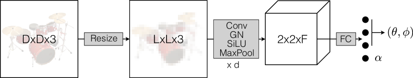
Figure S4: Architecture of the encoder. GN = group normalization [73], SiLU = Sigmoid Linear Unit [22], FC = fully connected layer. We map three of the outputs of the encoder to an azimuth/elevation pair $(\theta,\phi)$ using spherical coordinates. $D$ = input resolution, $L$ = encoder input resolution, $d$ = depth, $F$ = number of features. $\alpha$ is the camera roll, which we only predict for real datasets. Optionally, we can add three output dimensions to predict $T_{i}$, the location of the origin in the camera reference frame.

C.2 Encoder Ablations

We perform a series of ablations to explore encoder architecture. We run MELON on all training views of “lego”, “drum”, “ficus” and “ship” at $400\times 400$ resolution and $N=2$. We observe in our primary experiments that when poses converge, they tend to do so very quickly, often in the first thousand steps. We therefore train each configuration for 10k steps, but repeat 10 times to find min, max and mean metrics. We compute metrics as in other experiments over all test views. We choose a primary configuration of $L=64$, $F=32$, $d=4$ varying one parameter at a time in our experiments.

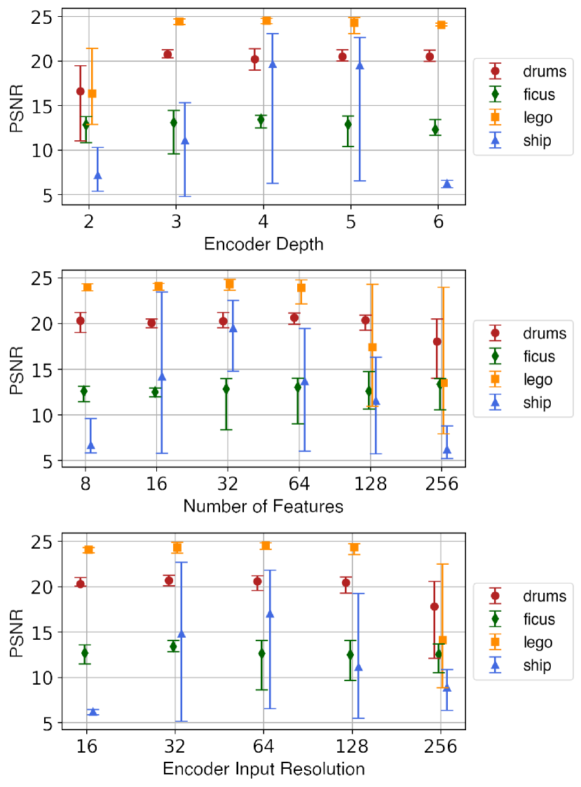
Figure S5: PSNR of novel view synthesis vs. encoder depth $d$, number of features $F$, and input resolution $L$, for four “NeRF-Synthetic” scenes. We report min, max and mean values over 10 runs.

Fig. S5 shows the result of sweeping feature count $F$ from 8 to 256 and encoder depth $d$ from 2 to 6 layers. We observe optimal values at 4 layers, and a feature count of 32.

Fig. S5 also shows performance sweeping encoder input resolutions $L$ from $16\times 16$ to $256\times 256$. We observe that certain datasets appear to work better at different resolutions, with optimal values typically ranging from $32\times 32$ to $128\times 128$. We therefore choose per-scene values in our primary experiments.

C.3 Replication Order

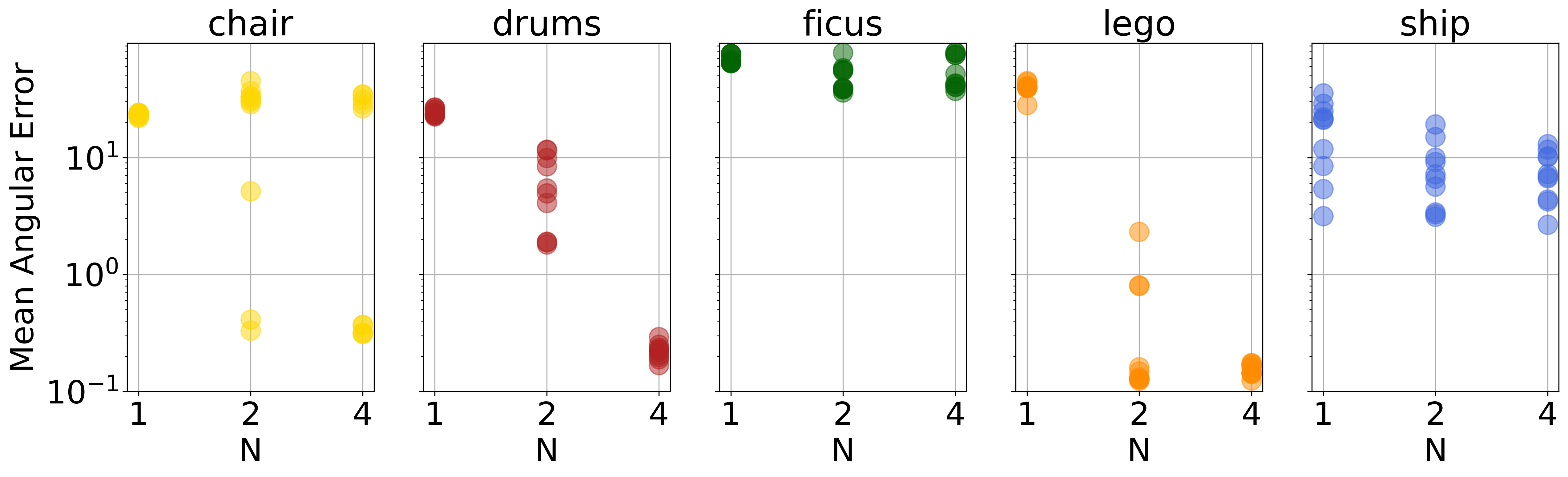
Figure S6: Scatter plot of the mean angular error vs. replication order $N$ for various “NeRF-Synthetic” scenes. We run each scene 10 times to 10k steps.

To determine the effect of varying the replication order, we run with the same base configuration as Sec. C.2, but varying replication order over $N=\{1,2,4\}$. We run MELON 10 times to 10k steps on five scenes and plot the results in Fig. S6. We observe a clear bi-modal behavior of convergence / non-convergence, and likelier convergence with higher $N$, consistent with our analysis of Sec. 3.4. The scenes “ficus” and “ship” typically take longer than 10k steps to converge, and thus are not well illustrated by this study.

C.4 Neural Radiance Field

We use the standard NeRF architecture of [44], an MLP with 8 layers of 256 features, and one skip connection to layer 4. Our density and RGB branches use a single layer of 128 channels. We use a single MLP, sampled at 96 stratified points, plus 32 additional importance sampled points, guided by the initial stratified samples. We keep the $t_{f}-t_{n}$ span fixed at 3.0 for baseline NeRF runs with ground truth cameras. For MELON runs, we linearly interpolate from 1.0 to 3.0 during the first 10k steps, which we found to aid convergence. We ignore view dependence for the first 50k steps by providing random view directions to the network. After 50k steps, we anneal a maximum of 4 frequency bands of directional encoding, until training completion at 100k steps. We use the Adam optimizer [31] with a learning rate of $10^{-4}$, $\beta_{1}=0.9,\beta_{2}=0.999$ and $128$ pixels per batch.

Appendix D Additional Results

D.1 Lego Scene

We show the self-similarity map and the regions of attraction of the Lego scene for a fixed elevation and a variable reference pose $z^{*}$ in Fig. S7.

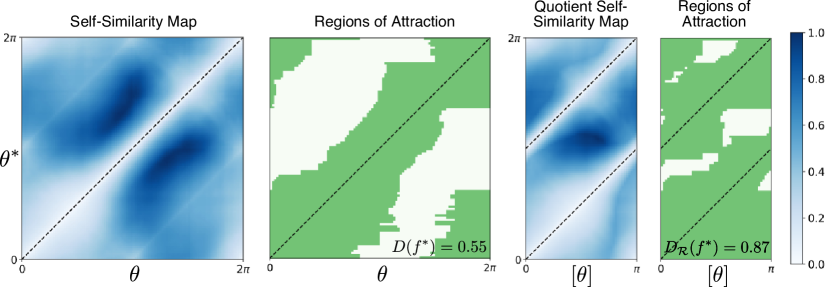
Figure S7: We generate 100 views of the “lego” scene with from an elevation $\phi\simeq 7^{\circ}$ and an azimuth $\theta\in[0^{\circ},360^{\circ}]$. The (normalized) self-similarity map $\mathcal{S}_{f^{*}}$ shows that the views taken from opposite sides look similar, due to the presence of rotationally symmetric elements in the bulldozer. The regions of attraction $K_{f^{*}}(\theta^{*})$ are colored in green. They only partially cover the latent space ($D(f^{*})=0.55$, higher is better, see (10)). With the equivalence relation $\mathcal{R}=\mathcal{R}_{2}$, the regions of attraction cover the quotient space $\Omega/\mathcal{R}$ almost entirely ($D_{\mathcal{R}}(f^{*})=0.87$, see (17)). Black dotted lines correspond to $\theta^{*}\in[\theta]$.

D.2 Comparison to VMRF

In our comparison to VMRF, the predicted elevation is constrained to the range $[-30^{\circ},90^{\circ}]$, as done in [77]. MELON achieves higher reconstruction metrics on all the “NeRF-Synthetic” scenes (Table S3).

D.3 Number of Views

We show qualitative reconstructions obtained on the “lego” dataset with a varying number of views in the training set in Fig. S9.

D.4 NeRF in the Wild

We report quantitative metrics obtains on the real datasets in Table S4 and qualitative reconstructions in Fig. S10.

	GNeRF		SAMURAI*		MELON		SAMURAI		NeRF
Scene	Rot. (∘)	PSNR	Rot. (∘)	PSNR	Rot. (∘)	PSNR	Rot. (∘)	PSNR	PSNR
Cape	56	16.3	56	12.9	1.5	19.5	5.1	20.6	19.1
Head	42	14.5	46	19.0	2.0	20.6	7.1	23.5	24.3
Toytruck	45	13.6	54	15.6	2.5	23.5	3.4	22.2	26.2

Table S4: Mean angular error on predicted poses (training set) and quality of novel view synthesis (test set). SAMURAI* uses a fixed initialization of the poses at the North pole while SAMURAI uses a manual rough initialization. “NeRF” is our implementation using published poses, provided by COLMAP. SAMURAI can achieve a better reconstruction thanks to a more flexible 3D representation (shape, BRDF and per-camera illumination), in spite of less accurate predicted poses. As ground truth poses are provided by COLMAP, angular errors may be noisy estimates of the true pose accuracy.

D.5 Noise Sensitivity

We compare MELON to COLMAP and GNeRF on noisy datasets. We add pixel-independent Gaussian noise of variance $\sigma^{2}$ to the training images and evaluate the mean angular error and novel view synthesis accuracy of competing methods in Table S3. We show a qualitative comparison between MELON and GNeRF in Fig. S8.

Noise	Pose Estimation			Novel View Synthesis
Std. Dev.	Rotation (∘)$\downarrow$			PSNR$\uparrow$
$\sigma$	COLMAP	GNeRF	MELON	GNeRF	MELON
0.125	fails	2.351	0.119	30.15	30.25
0.25	fails	4.271	0.190	27.32	28.62
0.5	fails	5.883	0.363	24.95	26.66
1.0	fails	7.557	1.784	22.90	24.20
2.0	fails	31.06	8.416	17.12	19.99

Table S5: Pose estimation accuracy and novel view synthesis quality of competing methods on the noisy “lego” scene. We report the best of three runs.

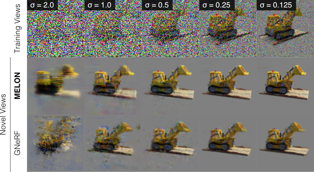
Figure S8: Novel view synthesis from noisy unposed images ($128\times 128$). Comparison between MELON and GNeRF.

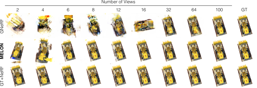
Figure S9: Qualitative reconstructions for various numbers of training views on the “lego” scene.

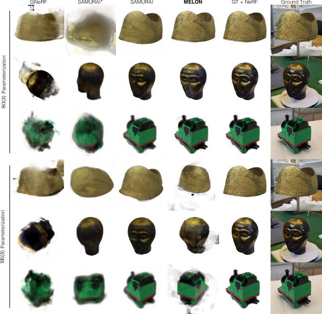
Figure S10: Additional qualitative results on the real datasets. Ground truth (GT) poses are provided by COLMAP. SAMURAI* uses a fixed initialization of the poses at the North pole while SAMURAI uses a manual coarse initialization. With the $\text{SO}(3)$ parameterization, the object-to-camera distances and the camera in-plane translations are assumed to be known.

References

- Batzner et al. [2022] Simon Batzner, Albert Musaelian, Lixin Sun, Mario Geiger, Jonathan P Mailoa, Mordechai Kornbluth, Nicola Molinari, Tess E Smidt, and Boris Kozinsky. E (3)-equivariant graph neural networks for data-efficient and accurate interatomic potentials. Nature communications, 13(1):1–11, 2022.
- Bepler et al. [2019] Tristan Bepler, Ellen Zhong, Kotaro Kelley, Edward Brignole, and Bonnie Berger. Explicitly disentangling image content from translation and rotation with spatial-vae. Advances in Neural Information Processing Systems, 32, 2019.
- Bian et al. [2022] Wenjing Bian, Zirui Wang, Kejie Li, Jia-Wang Bian, and Victor Adrian Prisacariu. Nope-nerf: Optimising neural radiance field with no pose prior. arXiv preprint arXiv:2212.07388, 2022.
- Boss et al. [2022] Mark Boss, Andreas Engelhardt, Abhishek Kar, Yuanzhen Li, Deqing Sun, Jonathan T Barron, Hendrik Lensch, and Varun Jampani. Samurai: Shape and material from unconstrained real-world arbitrary image collections. arXiv preprint arXiv:2205.15768, 2022.
- Bray and Dean [2007] Alan J Bray and David S Dean. Statistics of critical points of gaussian fields on large-dimensional spaces. Physical review letters, 98(15):150201, 2007.
- Chan et al. [2021] Eric Chan, Marco Monteiro, Peter Kellnhofer, Jiajun Wu, and Gordon Wetzstein. pi-GAN: Periodic Implicit Generative Adversarial Networks for 3D-Aware Image Synthesis. In CVPR, 2021.
- Chan et al. [2022] Eric R Chan, Connor Z Lin, Matthew A Chan, Koki Nagano, Boxiao Pan, Shalini De Mello, Orazio Gallo, Leonidas J Guibas, Jonathan Tremblay, Sameh Khamis, et al. Efficient geometry-aware 3d generative adversarial networks. In CVPR, pages 16123–16133, 2022.
- Chen et al. [2022a] Anpei Chen, Zexiang Xu, Andreas Geiger, Jingyi Yu, and Hao Su. Tensorf: Tensorial radiance fields. In ECCV, pages 333–350. Springer, 2022a.
- Chen et al. [2021] Haiwei Chen, Shichen Liu, Weikai Chen, Hao Li, and Randall Hill. Equivariant point network for 3d point cloud analysis. In CVPR, pages 14514–14523, 2021.
- Chen et al. [2022b] Shu Chen, Yang Zhang, Yaxin Xu, and Beiji Zou. Structure-aware nerf without posed camera via epipolar constraint. arXiv preprint arXiv:2210.00183, 2022b.
- Chng et al. [2022] Shin-Fang Chng, Sameera Ramasinghe, Jamie Sherrah, and Simon Lucey. Garf: Gaussian activated radiance fields for high fidelity reconstruction and pose estimation. arXiv e-prints, pages arXiv–2204, 2022.
- Community [2018] Blender Online Community. Blender - a 3D modelling and rendering package. Blender Foundation, Stichting Blender Foundation, Amsterdam, 2018.
- Dauphin et al. [2014] Yann N Dauphin, Razvan Pascanu, Caglar Gulcehre, Kyunghyun Cho, Surya Ganguli, and Yoshua Bengio. Identifying and attacking the saddle point problem in high-dimensional non-convex optimization. Advances in neural information processing systems, 27, 2014.
- Deng et al. [2021] Congyue Deng, Or Litany, Yueqi Duan, Adrien Poulenard, Andrea Tagliasacchi, and Leonidas J Guibas. Vector neurons: A general framework for so (3)-equivariant networks. In ICCV, pages 12200–12209, 2021.
- Elesedy and Zaidi [2021] Bryn Elesedy and Sheheryar Zaidi. Provably strict generalisation benefit for equivariant models. In ICML, pages 2959–2969. PMLR, 2021.
- Esteves et al. [2018] Carlos Esteves, Christine Allen-Blanchette, Ameesh Makadia, and Kostas Daniilidis. Learning so (3) equivariant representations with spherical cnns. In ECCV, pages 52–68, 2018.
- Esteves et al. [2019] Carlos Esteves, Yinshuang Xu, Christine Allen-Blanchette, and Kostas Daniilidis. Equivariant multi-view networks. In ICCV, pages 1568–1577, 2019.
- Falorsi et al. [2018] Luca Falorsi, Pim De Haan, Tim R Davidson, Nicola De Cao, Maurice Weiler, Patrick Forré, and Taco S Cohen. Explorations in homeomorphic variational auto-encoding. arXiv preprint arXiv:1807.04689, 2018.
- Fridovich-Keil et al. [2022] Sara Fridovich-Keil, Alex Yu, Matthew Tancik, Qinhong Chen, Benjamin Recht, and Angjoo Kanazawa. Plenoxels: Radiance fields without neural networks. In CVPR, pages 5501–5510, 2022.
- Fuchs et al. [2020] Fabian Fuchs, Daniel Worrall, Volker Fischer, and Max Welling. Se (3)-transformers: 3d roto-translation equivariant attention networks. Advances in Neural Information Processing Systems, 33:1970–1981, 2020.
- Gafni et al. [2021] Guy Gafni, Justus Thies, Michael Zollhöfer, and Matthias Nießner. Dynamic Neural Radiance Fields for Monocular 4D Facial Avatar Reconstruction. In CVPR, 2021.
- Hendrycks and Gimpel [2016] Dan Hendrycks and Kevin Gimpel. Gaussian error linear units (gelus). arXiv preprint arXiv:1606.08415, 2016.
- Henzler et al. [2019] Philipp Henzler, Niloy J Mitra, and Tobias Ritschel. Escaping plato’s cave: 3d shape from adversarial rendering. In ICCV, pages 9984–9993, 2019.
- Hu et al. [2020] Yinlin Hu, Pascal Fua, Wei Wang, and Mathieu Salzmann. Single-stage 6d object pose estimation. In CVPR, pages 2930–2939, 2020.
- Iglhaut et al. [2019] Jakob Iglhaut, Carlos Cabo, Stefano Puliti, Livia Piermattei, James O’Connor, and Jacqueline Rosette. Structure from motion photogrammetry in forestry: A review. Current Forestry Reports, 5:155–168, 2019.
- Jain et al. [2021] Ajay Jain, Matthew Tancik, and Pieter Abbeel. Putting NeRF on a Diet: Semantically Consistent Few-Shot View Synthesis. In ICCV, 2021.
- Jeong et al. [2021] Yoonwoo Jeong, Seokjun Ahn, Christopher Choy, Anima Anandkumar, Minsu Cho, and Jaesik Park. Self-calibrating neural radiance fields. In ICCV, pages 5846–5854, 2021.
- Kajiya and Von Herzen [1984] James T Kajiya and Brian P Von Herzen. Ray tracing volume densities. ACM SIGGRAPH computer graphics, 18(3):165–174, 1984.
- Kendall and Cipolla [2017] Alex Kendall and Roberto Cipolla. Geometric loss functions for camera pose regression with deep learning. In CVPR, pages 5974–5983, 2017.
- Kendall et al. [2015] Alex Kendall, Matthew Grimes, and Roberto Cipolla. Posenet: A convolutional network for real-time 6-dof camera relocalization. In ICCV, pages 2938–2946, 2015.
- Kingma and Ba [2014] Diederik P Kingma and Jimmy Ba. Adam: A method for stochastic optimization. arXiv preprint arXiv:1412.6980, 2014.
- Klee et al. [2023] David Klee, Ondrej Biza, Robert Platt, and Robin Walters. Image to icosahedral projection for so (3) object reasoning from single-view images. In NeurIPS Workshop on Symmetry and Geometry in Neural Representations, pages 64–80. PMLR, 2023.
- Levy et al. [2022a] Axel Levy, Frédéric Poitevin, Julien Martel, Youssef Nashed, Ariana Peck, Nina Miolane, Daniel Ratner, Mike Dunne, and Gordon Wetzstein. Cryoai: Amortized inference of poses for ab initio reconstruction of 3d molecular volumes from real cryo-em images. In ECCV, pages 540–557. Springer, 2022a.
- Levy et al. [2022b] Axel Levy, Gordon Wetzstein, Julien N. P. Martel, Frederic P. Poitevin, and Ellen D. Zhong. Amortized Inference for Heterogeneous Reconstruction in Cryo-EM. Advances in Neural Information Processing Systems, 2022b.
- Li et al. [2022] Tianye Li, Mira Slavcheva, Michael Zollhoefer, Simon Green, Christoph Lassner, Changil Kim, Tanner Schmidt, Steven Lovegrove, Michael Goesele, Richard Newcombe, et al. Neural 3d video synthesis from multi-view video. In CVPR, pages 5521–5531, 2022.
- Li et al. [2019] Zhigang Li, Yuwang Wang, and Xiangyang Ji. Monocular viewpoints estimation for generic objects in the wild. IEEE Access, 7:94321–94331, 2019.
- Lian et al. [2022] Ruyi Lian, Bingyao Huang, Liguo Wang, Qun Liu, Yuewei Lin, and Haibin Ling. End-to-end orientation estimation from 2d cryo-em images. Acta Crystallographica Section D: Structural Biology, 78(2), 2022.
- Lin et al. [2021] Chen-Hsuan Lin, Wei-Chiu Ma, Antonio Torralba, and Simon Lucey. BARF: Bundle-Adjusting Neural Radiance Fields. In ICCV, 2021.
- Lin et al. [2022] Yunzhi Lin, Thomas Müller, Jonathan Tremblay, Bowen Wen, Stephen Tyree, Alex Evans, Patricio A Vela, and Stan Birchfield. Parallel inversion of neural radiance fields for robust pose estimation. arXiv preprint arXiv:2210.10108, 2022.
- Lopez et al. [2019] Manuel Lopez, Roger Mari, Pau Gargallo, Yubin Kuang, Javier Gonzalez-Jimenez, and Gloria Haro. Deep single image camera calibration with radial distortion. In CVPR, pages 11817–11825, 2019.
- Mahendran et al. [2017] Siddharth Mahendran, Haider Ali, and René Vidal. 3d pose regression using convolutional neural networks. In ICCV Workshops, pages 2174–2182, 2017.
- Martin-Brualla et al. [2021] Ricardo Martin-Brualla, Noha Radwan, Mehdi S. M. Sajjadi, Jonathan Barron, Alexey Dosovitskiy, and Daniel Duckworth. NeRF in the Wild: Neural Radiance Fields for Unconstrained Photo Collections. In CVPR, 2021.
- Meng et al. [2021] Quan Meng, Anpei Chen, Haimin Luo, Minye Wu, Hao Su, Lan Xu, Xuming He, and Jingyi Yu. Gnerf: Gan-based neural radiance field without posed camera. In ICCV, pages 6351–6361, 2021.
- Mildenhall et al. [2020] Ben Mildenhall, Pratul Srinivasan, Matthew Tancik, Jonathan Barron, Ravi Ramamoorthi, and Ren Ng. NeRF: Representing Scenes as Neural Radiance Fields for View Synthesis. In ECCV, pages 405–421. Springer, 2020.
- Mildenhall et al. [2022] Ben Mildenhall, Peter Hedman, Ricardo Martin-Brualla, Pratul P Srinivasan, and Jonathan T Barron. Nerf in the dark: High dynamic range view synthesis from noisy raw images. In CVPR, pages 16190–16199, 2022.
- Müller et al. [2022] Thomas Müller, Alex Evans, Christoph Schied, and Alexander Keller. Instant neural graphics primitives with a multiresolution hash encoding. ACM Transactions on Graphics (ToG), 41(4):1–15, 2022.
- Murphy et al. [2021] Kieran Murphy, Carlos Esteves, Varun Jampani, Srikumar Ramalingam, and Ameesh Makadia. Implicit-pdf: Non-parametric representation of probability distributions on the rotation manifold. arXiv preprint arXiv:2106.05965, 2021.
- Nasiri and Bepler [2022] Alireza Nasiri and Tristan Bepler. Unsupervised object representation learning using translation and rotation group equivariant vae. arXiv preprint arXiv:2210.12918, 2022.
- Nguyen-Phuoc et al. [2019] Thu Nguyen-Phuoc, Chuan Li, Lucas Theis, Christian Richardt, and Yong-Liang Yang. Hologan: Unsupervised learning of 3d representations from natural images. In ICCV, pages 7588–7597, 2019.
- Niemeyer and Geiger [2021a] Michael Niemeyer and Andreas Geiger. Giraffe: Representing scenes as compositional generative neural feature fields. In CVPR, pages 11453–11464, 2021a.
- Niemeyer and Geiger [2021b] Michael Niemeyer and Andreas Geiger. GIRAFFE: Representing Scenes as Compositional Generative Neural Feature Fields. In CVPR, 2021b.
- Noguchi [2021] Atsuhiro Noguchi. Neural Articulated Radiance Field. In ICCV, 2021.
- Özyeşil et al. [2017] Onur Özyeşil, Vladislav Voroninski, Ronen Basri, and Amit Singer. A survey of structure from motion*. Acta Numerica, 26:305–364, 2017.
- Park et al. [2021] Keunhong Park, Utkarsh Sinha, Jonathan Barron, Sofien Bouaziz, Dan Goldman, Steven Seitz, and Ricardo Martin-Brualla. Nerfies: Deformable Neural Radiance Fields. In ICCV, 2021.
- Pett [2016] Daniel Pett. Ethiopian head. 2016.
- Pett [2017] Daniel Pett. Britishmuseumdh/moldgoldcape: First release of the cape in 3d. 2017.
- Raj et al. [2021] Amit Raj, Michael Zollhofer, Tomas Simon, Jason Saragih, Shunsuke Saito, James Hays, and Stephen Lombardi. Pixel-aligned volumetric avatars. In CVPR, pages 11733–11742, 2021.
- Rebain et al. [2020] Daniel Rebain, Wei Jiang, Soroosh Yazdani, Ke Li, Kwang Moo Yi, and Andrea Tagliasacchi. DeRF: Decomposed Radiance Fields. https://arxiv.org/abs/2011.12490, 2020.
- Reiser et al. [2021] Christian Reiser, Songyou Peng, Yiyi Liao, and Andreas Geiger. KiloNeRF: Speeding Up Neural Radiance Fields With Thousands of Tiny MLPs. In ICCV, 2021.
- Reizenstein [2021] Jeremy Reizenstein. Common Objects in 3D: Large-Scale Learning and Evaluation of Real-life 3D Category Reconstruction. In ICCV, 2021.
- Reizenstein et al. [2021] Jeremy Reizenstein, Roman Shapovalov, Philipp Henzler, Luca Sbordone, Patrick Labatut, and David Novotny. Common objects in 3d: Large-scale learning and evaluation of real-life 3d category reconstruction. In ICCV, pages 10901–10911, 2021.
- Sattler et al. [2019] Torsten Sattler, Qunjie Zhou, Marc Pollefeys, and Laura Leal-Taixe. Understanding the limitations of cnn-based absolute camera pose regression. In CVPR, pages 3302–3312, 2019.
- Schonberger and Frahm [2016] Johannes L Schonberger and Jan-Michael Frahm. Structure-from-motion revisited. In CVPR, pages 4104–4113, 2016.
- Shekarforoush et al. [2022] Shayan Shekarforoush, David B Lindell, David J Fleet, and Marcus A Brubaker. Residual multiplicative filter networks for multiscale reconstruction. arXiv preprint arXiv:2206.00746, 2022.
- Sinha et al. [2022] Samarth Sinha, Jason Y Zhang, Andrea Tagliasacchi, Igor Gilitschenski, and David B Lindell. Sparsepose: Sparse-view camera pose regression and refinement. arXiv preprint arXiv:2211.16991, 2022.
- Su et al. [2015] Hao Su, Charles R Qi, Yangyan Li, and Leonidas J Guibas. Render for cnn: Viewpoint estimation in images using cnns trained with rendered 3d model views. In ICCV, pages 2686–2694, 2015.
- Sucar et al. [2021] Edgar Sucar, Shikun Liu, Joseph Ortiz, and Andrew Davison. iMAP: Implicit Mapping and Positioning in Real-Time. In ICCV, 2021.
- Sun et al. [2022] Cheng Sun, Min Sun, and Hwann-Tzong Chen. Direct voxel grid optimization: Super-fast convergence for radiance fields reconstruction. In CVPR, pages 5459–5469, 2022.
- Truong et al. [2022] Prune Truong, Marie-Julie Rakotosaona, Fabian Manhardt, and Federico Tombari. Sparf: Neural radiance fields from sparse and noisy poses. arXiv preprint arXiv:2211.11738, 2022.
- Wang et al. [2022] Liao Wang, Jiakai Zhang, Xinhang Liu, Fuqiang Zhao, Yanshun Zhang, Yingliang Zhang, Minye Wu, Jingyi Yu, and Lan Xu. Fourier plenoctrees for dynamic radiance field rendering in real-time. In CVPR, pages 13524–13534, 2022.
- Wang et al. [2004] Zhou Wang, Alan C Bovik, Hamid R Sheikh, and Eero P Simoncelli. Image quality assessment: from error visibility to structural similarity. IEEE transactions on image processing, 13(4):600–612, 2004.
- Wang et al. [2021] Zirui Wang, Shangzhe Wu, Weidi Xie, Min Chen, and Victor Adrian Prisacariu. NeRF–: Neural Radiance Fields Without Known Camera Parameters. https://arxiv.org/abs/2102.07064, 2021.
- Wu and He [2018] Yuxin Wu and Kaiming He. Group normalization. In ECCV, pages 3–19, 2018.
- Xu et al. [2022] Dejia Xu, Yifan Jiang, Peihao Wang, Zhiwen Fan, Humphrey Shi, and Zhangyang Wang. Sinnerf: Training neural radiance fields on complex scenes from a single image. In ECCV, pages 736–753. Springer, 2022.
- Yen-Chen et al. [2021] Lin Yen-Chen, Pete Florence, Jonathan Barron, Alberto Rodriguez, Phillip Isola, and Tsung-Yi Lin. iNeRF: Inverting Neural Radiance Fields for Pose Estimation. In IROS, 2021.
- Yu et al. [2021] Alex Yu, Vickie Ye, Matthew Tancik, and Angjoo Kanazawa. pixelNeRF: Neural Radiance Fields from One or Few Images. In CVPR, 2021.
- Zhang et al. [2022a] Jiahui Zhang, Fangneng Zhan, Rongliang Wu, Yingchen Yu, Wenqing Zhang, Bai Song, Xiaoqin Zhang, and Shijian Lu. Vmrf: View matching neural radiance fields. In Proceedings of the 30th ACM International Conference on Multimedia, pages 6579–6587, 2022a.
- Zhang et al. [2022b] Jason Y Zhang, Deva Ramanan, and Shubham Tulsiani. Relpose: Predicting probabilistic relative rotation for single objects in the wild. In ECCV, pages 592–611. Springer, 2022b.
- Zhang et al. [2018] Richard Zhang, Phillip Isola, Alexei A Efros, Eli Shechtman, and Oliver Wang. The unreasonable effectiveness of deep features as a perceptual metric. In CVPR, 2018.
- Zhong et al. [2021] Ellen D Zhong, Tristan Bepler, Bonnie Berger, and Joseph H Davis. Cryodrgn: reconstruction of heterogeneous cryo-em structures using neural networks. Nature methods, 18(2):176–185, 2021.
- Zhu et al. [2022] Zihan Zhu, Songyou Peng, Viktor Larsson, Weiwei Xu, Hujun Bao, Zhaopeng Cui, Martin R Oswald, and Marc Pollefeys. Nice-slam: Neural implicit scalable encoding for slam. In CVPR, pages 12786–12796, 2022.