Cosmoglobe DR1 results. I. Improved Wilkinson Microwave Anisotropy Probe maps through Bayesian end-to-end analysis

We present Cosmoglobe Data Release 1, which implements the first joint analysis of WMAP and Planck LFI time-ordered data, processed within a single Bayesian end-to-end framework. This framework builds directly on a similar analysis of the LFI measurements by the BeyondPlanck collaboration, and approaches the CMB analysis challenge through Gibbs sampling of a global posterior distribution, simultaneously accounting for calibration, mapmaking, and component separation. The computational cost of producing one complete WMAP+LFI Gibbs sample is 812 CPU-hr, of which 603 CPU-hrs are spent on WMAP low-level processing; this demonstrates that end-to-end Bayesian analysis of the WMAP data is computationally feasible. We find that our WMAP posterior mean temperature sky maps and CMB temperature power spectrum are largely consistent with the official WMAP9 results. Perhaps the most notable difference is that our CMB dipole amplitude is $3366.2\pm 1.4\thinspace\mathrm{\mu K}$, which is 11 $\mu$K higher than the WMAP9 estimate and $2.5\thinspace\sigma$ higher than BeyondPlanck; however, it is in perfect agreement with the HFI-dominated Planck PR4 result. In contrast, our WMAP polarization maps differ more notably from the WMAP9 results, and in general exhibit significantly lower large-scale residuals. We attribute this to a better constrained gain and transmission imbalance model. It is particularly noteworthy that the W-band polarization sky map, which was excluded from the official WMAP cosmological analysis, for the first time appears visually consistent with the V-band sky map. Similarly, the long standing discrepancy between the WMAP K-band and LFI 30 GHz maps is finally resolved, and the difference between the two maps appears consistent with instrumental noise at high Galactic latitudes. Relatedly, these updated maps allow us for the first time to combine WMAP and LFI polarization data into a single coherent model of large-scale polarized synchrotron emission. Still, we identify a few issues that require additional work, including 1) low-level noise modeling, 2) large-scale temperature residuals at the 1–2 $\mu$K level; and 3) a strong degeneracy between the absolute $K$-band calibration and the dipole of the anomalous microwave emission component. We conclude that leveraging the complementary strengths of WMAP and LFI has allowed the mitigation of both experiments’ weaknesses, and resulted in new state-of-the-art WMAP sky maps. All maps and the associated code are made publicly available through the Cosmoglobe web page.

1 Introduction

The discovery of the cosmic microwave background (CMB) by Penzias & Wilson (1965) marked a paradigm shift in the field of cosmology, providing direct evidence that the Universe was once much hotter than it is today, effectively ruling out the steady-state theory of the universe (Dicke et al. 1965). This discovery spurred a series of ground-breaking cosmological experiments, including the Nobel Prize-winning measurements by COBE-FIRAS that confirmed the blackbody nature of the CMB (Mather et al. 1994) and COBE-DMR that measured temperature variations from the primordial gravitational field (Smoot et al. 1992).

The NASA-funded Wilkinson Microwave Anisotropy Probe (WMAP; Bennett et al. 2003a) mission was launched a decade after COBE-DMR, and mapped the microwave sky with 45 times higher sensitivity and 33 times higher angular resolution, thereby revolutionizing our understanding of early universe physics (Bennett et al. 2003a). In addition, the 3-year measurements presented by Page et al. (2007) included the first ever detection of large-scale polarization in the CMB, opening a new window into the process of cosmic reionization. As quantified by Bennett et al. (2013), the permissible parameter space volume for a standard $\Lambda$CDM model was decreased by a factor of 68,000 by WMAP, and the best pre-WMAP determination of the age of the universe was $t_{0}<14\thinspace\mathrm{Gyr}$ from Boomerang (Lange et al. 2001), with best-fit values of 9–11 Gyr; the latter values in apparent contradiction with direct measurements of the oldest globular clusters (Hu et al. 2001).

The ESA-led Planck satellite (Planck Collaboration I 2020) was developed concurrently with WMAP, and their operation lifetimes partially overlapped, with WMAP observing from 2001–2011 and Planck from 2009–2013. Planck’s stated goal was to fully characterize the primary CMB temperature fluctuations from recombination, as well as to characterize the polarized microwave sky on large angular scales. Overall, Planck’s raw CMB sensitivity was an order of magnitude higher than WMAP’s, and its angular resolution more than twice higher. Today, Planck represents the state-of-the-art in terms of full-sky microwave sky measurements.

Planck comprised two independent experiments, namely the Low Frequency Instrument (LFI; Planck Collaboration II 2020) and High Frequency Instrument (HFI; Planck Collaboration III 2020), respectively. The LFI detectors were based on HEMT (high electron mobility transistor) amplifiers, spanning three frequency channels between 30 and 70 GHz, while the HFI detectors were based on spider-web and polarization sensitive bolometers, and spanned six frequency channels between 100 and 857 GHz. For comparison, WMAP was also HEMT-based, with comparable sensitivity to LFI alone, and spanned five frequencies between 23 and 94 GHz. At the same time, the two experiments implemented very different scanning strategies, and as a result they are highly complementary and synergistic; together they provide a clearer view of the low-frequency microwave sky than either can alone.

Towards the end of the Planck analysis phase it became clear that the interplay between instrument calibration and astrophysical component separation was a main limiting factor in terms of systematic effects for high signal-to-noise measurements (Planck Collaboration II 2020). Specifically, in order to calibrate the instrument to sufficient precision, it became apparent that it was necessary to know the true sky to a comparably high precision – but to know the sky, it was also necessary to know the instrumental calibration. The data analysis was thus fundamentally circular and global in nature. The final official Planck LFI analysis performed four complete iterations between calibration and component separation (Planck Collaboration II 2020), aiming to probe this degeneracy. However, it was recognized that this was not sufficient to reach full convergence, and this sub-optimality led to the BeyondPlanck project (BeyondPlanck 2023), which aimed to perform thousands of complete analysis cycles, as opposed to just a handful. This framework was implemented using the Commander3 (Galloway et al. 2023a) code, a CMB Gibbs sampler that performs integrated high-level and low-level parameter estimation in a single integrated framework. This analysis demonstrated the feasibility of end-to-end CMB analysis through Gibbs sampling analysis, while at the same time it provided the highest-quality LFI maps to date.

Rather than simply probing the degeneracy between instrument calibration and component separation, a better solution is to actually break it. The optimal approach to do so is by jointly analyzing complementary datasets, each of which provide key information regarding the full system. This insight led to the Cosmoglobe initiative, which is an Open Source and community-wide effort that aims to derive a single joint model of the radio, microwave, and sub-millimeter sky by combining all available state-of-the-art experiments. An obvious first extension of the LFI-oriented BeyondPlanck project is to analyze the WMAP measurements in the same framework. Indeed, already as part of the BeyondPlanck suite of papers, Watts et al. (2023b) integrated WMAP Q-band time-ordered data (TOD) into the Commander3 framework, calibrated off of the BeyondPlanck sky model.

In this paper, we present the first end-to-end Bayesian analysis of the full WMAP TOD, processed within the Commander framework. As such, this paper also presents the first ever joint analysis of two major CMB experiments (LFI and WMAP) at the lowest possible level, and it therefore constitutes a major milestone of the Cosmoglobe initiative. We refer to the current products as Cosmoglobe Data Release 1 (CG1), and the scientific results from this are described in a series of four papers. The current paper gives a detailed discussion of data processing methods, instrumental parameters, frequency maps, and preliminary astrophysical results, while updated constraints on anomalous microwave emission and polarized synchrotron emission are presented by Watts et al. (2023a) and Fuskeland et al. (2023), respectively. Eskilt et al. (2023) use these new products to provide new constraints on cosmic birefringence. In the future, many more datasets and astrophysical components will be added to this framework, gradually providing stronger and stronger constraints on both the true astrophysical sky and the instrumental calibration of all previous experiments.

The rest of this paper is organized as follows. In Sect. 2, we provide a brief review of the Bayesian end-to-end statistical framework used in this work, before describing the underlying data and computational expenses in Sect. 3. The main results, as expressed by the global posterior distribution, are described in Sects. 4–6, summarizing instrumental parameters, frequency sky maps, and preliminary astrophysical results, respectively. In Sect. 7 we address unresolved issues that should be further analyzed in future work. We conclude in Sect. 8, and lay a path forward for the Cosmoglobe project.

2 End-to-end Bayesian CMB analysis

The general computational analysis framework used in this work has been described in detail by BeyondPlanck (2023) and Watts et al. (2023b) and references therein. In this section, we give a brief summary of the main points, and emphasize in particular the differences with respect to earlier work.

2.1 Official WMAP instrument model and analysis pipeline

The main goal of the current paper is to perform a similar analysis as BeyondPlanck (2023) did for Planck LFI, but this time including the WMAP in terms of time-ordered data, and thereby solve some of the long-standing unresolved issues with the official maps, in particular related to poorly constrained large-scale polarization modes. Before presenting our algorithm, however, it is useful to briefly review the official WMAP instrument model and analysis pipeline, which improved gradually over a total of five data releases, often referred to as the 1-, 3-, 5-, 7-, and 9-year data releases, respectively. Unless otherwise noted, we will refer to the final 9-year results (Bennett et al. 2013), and denote these as WMAP9. A concise summary of the WMAP mission, data processing, and results is available in Komatsu et al. (2014). The full data archive can be found on LAMBDA.

The WMAP satellite carried twenty differential polarization-sensitive radiometers, grouped into ten differencing assemblies (DAs), where one was sensitive to the difference in signal at one polarization orientation and the other sensitive to the orthogonal polarization. In total, of the ten DAs there were: one K-band (23 GHz), one Ka-band (33 GHz), two Q-bands (41 GHz), two V-bands (61 GHz), and four W-bands (94 GHz). Each radiometer comprised two detector diodes, which each recorded a science sample every $1.536/N_{\mathrm{obs}}$ seconds, where $N_{\mathrm{obs}}$ is 12, 12, 15, 20 and 30 for K, Ka, Q, V, and W, respectively. The raw data are recorded as 16-bit integers with units du (digital unit).

The WMAP bandpasses were measured pre-launch on the ground, sweeping a signal source through 201 frequencies and recording the output (Jarosik et al. 2003b). The bandpass responses available on LAMBDA have not been updated since the initial data release. However, as noted by Bennett et al. (2013), there has been an observed drift in the center frequency of K, Ka, Q, and V-band corresponding to a $\sim$$\thinspace 0.1\thinspace\%$ decrease over time. In practice, this did not affect the WMAP data processing because each year was mapped separately and co-added afterwards. An effective frequency calculator was delivered in the DR5 release as part of the IDL library to mitigate this effect during astrophysical analyses.

The beams were characterized in the form of maps, with separate products for the central portion of the beam pattern and the far sidelobes. The main beam and near sidelobes were characterized using a combination of physical optics codes and observations of Jupiter for each horn separately. The maps of Jupiter were then combined with the best-fit parameters from physical optics codes to create a map of the beam response (Hill et al. 2009; Weiland et al. 2011; Bennett et al. 2013).

Far sidelobes were estimated using a combination of laboratory measurements and Moon data taken during the mission (Barnes et al. 2003), as well as a physical optics model described by Hinshaw et al. (2009). To remove the far sidelobe in the TOD, an estimate was calculated by convolving the intensity map and the orbital dipole signal with the measured sidelobe signal (Jarosik et al. 2007). Although the sidelobe pickup was modeled by Barnes et al. (2003), it was determined that the results were small enough to be neglected and have not been explicitly reported in any of the subsequent WMAP data releases.

The WMAP pointing solution was determined using the boresight vectors of individual feedhorns in spacecraft coordinates, in combination with on-board star trackers. Thermal flexure of the tracking structure introduced small pointing errors, as discussed by Jarosik et al. (2007). Using the temperature variation measured by onboard thermistors, the pointing solution was corrected using a model that returns angular deviation per kelvin. The residual pointing errors were computed using observations of Jupiter and Saturn, and the reported upper limit was estimated to be 10″ (Greason et al. 2012; Bennett et al. 2013).

The WMAP data were calibrated by jointly estimating the time-dependent gains, $\@vec{g}$, and baselines, $\@vec{b}$, as described by Hinshaw et al. (2007), Hinshaw et al. (2009), and Jarosik et al. (2011). The TOD were initially modeled as having constant gain and baseline for a 1–24 hour period, with parameters that were fit to the orbital dipole assuming $T_{0}$ from Mather et al. (1999) and a map made from a previous iteration of the mapmaking procedure. Once the gain and baseline solution had converged, the data were fit to a parametric form of the radiometer response as a function of housekeeping data, given in Appendix A of Greason et al. (2012).

WMAP had two primary mirrors positioned on opposite sides of the vertical satellite axis, tilted approximately $19.5^{\circ}$ towards the Solar shield. Essentially, when horn A was pointed at pixel $p_{\mathrm{A}}$, horn B was pointed at a pixel $p_{\mathrm{B}}$ approximately $141^{\circ}$ away (Page et al. 2003). The incoming radiation was differenced in the electronics before being deposited on the detectors, recording radiation proportional to the observed maps $\boldsymbol{m}$ at their respective pixels, $\boldsymbol{m}_{p_{\mathrm{A}}}-\boldsymbol{m}_{p_{\mathrm{B}}}$ and $\boldsymbol{m}_{p_{\mathrm{B}}}-\boldsymbol{m}_{p_{\mathrm{A}}}$ (Jarosik et al. 2003b). Each radiometer had a partner that observed the same pixels with sensitivity to the orthogonal polarization direction. Taking all these effects into account, the total data model for a single radiometer is given by

$$d_{t}^{\mathrm{imbal}} \propto(1+x_{\mathrm{im}})T_{p_{\mathrm{A}}}-(1-x_{\mathrm{im}})T_{p_{\mathrm{B}}}$$ (1)

$$=(T_{p_{\mathrm{A}}}-T_{p_{\mathrm{B}}})+x_{\mathrm{im}}(T_{p_{\mathrm{A}}}+T_{p_{\mathrm{B}}}),$$ (2)

where $T_{p_{\mathrm{A}}}$ and $T_{p_{\mathrm{B}}}$ are the A- and B-side antenna temperatures, and $x_{\mathrm{im}}$ is the differential optical pickup between horns A and B. This effect is taken into account during mapmaking. However, inaccuracies in the determination of $x_{\mathrm{im}}$ will yield a spurious polarization component, and create artificial imbalance modes due to coupling with the sky signal, in particular with the bright Solar CMB dipole (Jarosik et al. 2007). The WMAP transmission imbalance factors were fit to the Solar dipole in TOD space, accounting for both common and differential modes (Jarosik et al. 2003a, 2007).

Data were flagged and masked before the final mapmaking step. In particular, station-keeping maneuvers, solar flares, and unscheduled events caused certain data to be unusable – the full catalog of these events is listed in Table 1.8 of Greason et al. (2012). In addition, data were masked depending on the channel frequency and the planet itself, with the full list of exclusion radii enumerated in Table 4 of Bennett et al. (2013).

To create the sky maps $\boldsymbol{m}$, the calibrated data were put into the asymmetric mapmaking equation,

$$\mathsf{P}_{\mathrm{am}}^{T}\mathsf{N}^{-1}\mathsf{P}\boldsymbol{m}=\mathsf{P}^{T}_{\mathrm{am}}\mathsf{N}^{-1}\boldsymbol{d},$$ (3)

where $\mathsf{N}$ is the noise covariance matrix, and the pointing matrix $\mathsf{P}$ is implicitly defined for each datastream, $\boldsymbol{d}_{1}$ and $\boldsymbol{d}_{2}$ sensitive to different polarization orientations. The asymmetric mapmaking matrix, $\mathsf{P}_{\mathrm{am}}$, was used because, as noted by Jarosik et al. (2011), large signals observed in one beam could leak into the solution for the pixel observed by the other beam, leading to incorrect signals in the final map. The asymmetric mapmaking solution is defined by only updating the matrix multiplication for beam A when beam A is in a high emission region and beam B is not, and vice versa. Bennett et al. (2013) also identified that these effects are pronounced when one horn is crossing a large temperature gradient, leading to excesses $140^{\circ}$ away from the Galactic center if an appropriate processing mask is not used. For each side $\mathrm{A}/\mathrm{B}$, the maps are defined as a function of the Stokes parameters $T_{\mathrm{A}/\mathrm{B}}$, $Q_{\mathrm{A}/\mathrm{B}}$, and $U_{\mathrm{A}/\mathrm{B}}$, with polarization angle $\gamma_{\mathrm{A}/\mathrm{B}}$, such that

$$\boldsymbol{d}_{1} =\mathsf{P}_{1}\boldsymbol{m}$$

$$=(1+x_{\mathrm{im}})[T_{\mathrm{A}}+Q_{\mathrm{A}}\cos 2\gamma_{\mathrm{A}}+U_{\mathrm{A}}\sin 2\gamma_{\mathrm{A}}+S_{\mathrm{A}}]$$

$$+(1-x_{\mathrm{im}})[-T_{\mathrm{B}}-Q_{\mathrm{B}}\cos 2\gamma_{\mathrm{B}}-U_{\mathrm{B}}\sin 2\gamma_{\mathrm{B}}-S_{\mathrm{B}}],$$ (4)

and

$$\boldsymbol{d}_{2} =\mathsf{P}_{2}\boldsymbol{m}$$

$$=(1+x_{\mathrm{im}})[T_{\mathrm{A}}-Q_{\mathrm{A}}\cos 2\gamma_{\mathrm{A}}-U_{\mathrm{A}}\sin 2\gamma_{\mathrm{A}}-S_{\mathrm{A}}]$$

$$+(1-x_{\mathrm{im}})[-T_{\mathrm{B}}+Q_{\mathrm{B}}\cos 2\gamma_{\mathrm{B}}+U_{\mathrm{B}}\sin 2\gamma_{\mathrm{B}}+S_{\mathrm{B}}].$$ (5)

In this formalism, $S_{\mathrm{A}/\mathrm{B}}$ acts as an extra Stokes parameter that absorbs the effects of differing bandpass responses between radiometers $\boldsymbol{d}_{1}$ and $\boldsymbol{d}_{2}$ (Jarosik et al. 2007).

An accurate noise model was necessary both to perform the maximum likelihood mapmaking and for the evaluation of the dense time-space inverse noise covariance matrix $\mathsf{N}^{-1}$. The WMAP team defined this in the form of a time domain autocorrelation function that was estimated separately for each year of data. This was then Fourier transformed, inverted, and inverse Fourier transformed to create an effective inverse noise operator $N_{tt^{\prime}}^{-1}$. Finally, to create the sky maps themselves, the WMAP team processed the data one year at a time, producing maps by solving Eq. (3) using the iterative Bi-Conjugate Gradient Stabilized Method (BiCG-STAB, van der Vorst 1992; Barrett et al. 1994).

2.2 Cosmoglobe instrument model

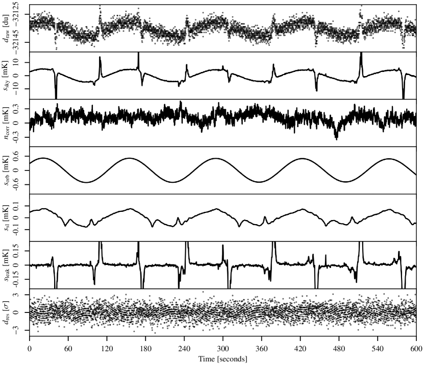
Figure 1: Time-ordered data segment for the K113 diode. From top to bottom, the panels show 1) raw uncalibrated TOD $\boldsymbol{d}$; 2) sky signal $\boldsymbol{s}_{\mathrm{sky}}$; 3) calibrated correlated noise $\boldsymbol{n}_{\mathrm{corr}}$; 4) orbital CMB dipole signal $\boldsymbol{s}_{\mathrm{orb}}$; 5) sidelobe correction $\boldsymbol{s}_{\mathrm{sl}}$; 6) bandpass leakage correction $\boldsymbol{s}_{\mathrm{leak}}$; and 7) residual TOD, $\boldsymbol{d}_{\mathrm{res}}=(\boldsymbol{d}-\boldsymbol{n}_{\mathrm{corr}}-\boldsymbol{b})/g-\boldsymbol{s}_{\mathrm{sky}}-\boldsymbol{s}_{\mathrm{orb}}-\boldsymbol{s}_{\mathrm{leak}}-\boldsymbol{s}_{\mathrm{sl}}$, in units of $\sigma_{0}[\mathrm{du}]$ for this TOD segment. Note that the vertical range varies and units vary from panel to panel.

A fundamental difference between the Cosmoglobe and WMAP analysis pipelines (and those of most other CMB experiments) is that while the WMAP pipeline models each channel in isolation, the Cosmoglobe framework simultaneously considers all data, both internally within WMAP, and also from all other sources, and most notably from Planck LFI. The main advantage of such a global approach is significantly reduced parameter degeneracies, as data from observations with different frequency coverages and instrumental designs break the same degeneracies. For this approach to be computationally tractable, one must establish a global parametric model that simultaneously accounts for both the astrophysical sky and all relevant instruments. For the current WMAP+LFI oriented analysis, we adopt the following expression (BeyondPlanck 2023),

$$\boldsymbol{d}=\mathsf{G}\mathsf{P}[\mathsf{B}^{\mathrm{symm}}\mathsf{M}\boldsymbol{a}+\mathsf{B}^{\mathrm{4\pi}}(\boldsymbol{s}^{\mathrm{orb}}+\boldsymbol{s}^{\mathrm{fsl}})]+\boldsymbol{s}^{\mathrm{inst}}+\boldsymbol{n}^{\mathrm{corr}}+\boldsymbol{n}^{\mathrm{w}},$$ (6)

where $\mathsf{G}$ is the time-dependent gain in the form of the matrix $\mathrm{diag}(g_{t})$; $\mathsf{P}$ is the $n_{p}\times n_{\mathrm{TOD}}$ pointing matrix, where $n_{p}$ is the number of pixels and $n_{\mathrm{TOD}}$ length of the TOD; $\mathsf{B}^{\mathrm{symm}}$ and $\mathsf{B}^{4\pi}$ are the symmetrized and full asymmetric beam, respectively; $\mathsf{M}$ is the mixing matrix between a given sky component $c$ with spectral energy distribution $f_{c}(\nu/\nu_{0,c})$ and a detector $i$ with bandpass $\tau_{i}(\nu)$, given by

$$\mathsf{M}_{ci}=\int d\nu\thinspace\tau_{i}(\nu)f_{c}(\nu/\nu_{c,0}).$$ (7)

(In practice, $\@tens{M}$ also accounts for unit conversion, but this is suppressed for readability in this expression; see Svalheim et al. 2023a for further details.) The maps $\boldsymbol{a}$ represent the Stokes parameters for each astrophysical component, while $\boldsymbol{s}^{\mathrm{orb}}$ is the orbital dipole induced by the motion of the telescope with respect to the Sun, and $\boldsymbol{s}^{\mathrm{fsl}}$ is the time-dependent far sidelobe signal. Following Ihle et al. (2023), we model the correlated noise component $\boldsymbol{n}^{\mathrm{corr}}$ in terms of a $1/f$ power spectral density (PSD), which explicitly takes the form $P_{n}(f)=\sigma^{2}_{0}(1+(f/f_{\mathrm{knee}})^{\alpha})$, where $\sigma_{0}$ denotes the white noise amplitude, $f_{\mathrm{knee}}$ is the so-called $1/f$ knee frequency, and $\alpha$ is a free power law slope. For notational purposes, we denote the set of all correlated noise parameters by $\boldsymbol{\xi}_{n}=\{\sigma_{0},f_{\mathrm{knee}},\alpha\}$. We note that this model represents a significant approximation compared to the more flexible WMAP autocorrelation model, as the actual WMAP noise is known to be colored at high temporal frequencies (Jarosik et al. 2007). The main impact of this approximation is a worse-than-expected $\chi^{2}$ goodness of fit statistic. However, measured in absolute noise levels the effect is very small, and has very little if any impact on the final science results; for further discussion of this approximation, see Sect. 7.1.

The term $\boldsymbol{s}^{\mathrm{inst}}$ denotes any instrument-specific terms that might be required for a given experiment. For instance, for LFI it is used to model the 1 Hz spike contribution due to electronic cross-talk. For WMAP, we use it for first-order baseline corrections, and set $s^{\mathit{WMAP}}_{t}=b_{0}+b_{1}\thinspace t$, where $b_{0}$ and $b_{1}$ represent the mean and slope of the baselines over the data segment in question. We note that while the WMAP team fitted a single constant baseline over either 1- or 24-hour periods, our data segments are typically several days long (corresponding to a number of samples chosen to optimize Fourier transforms). A natural question is therefore whether nonlinear baseline variations could induce artifacts. In this regard, it is important to note that the correlated noise component effectively acts as a single-sample baseline correction that can absorb by far most such nonlinearities, as long as their total effect on the power spectrum does not exceed that imposed by the $1/f$ model. In practice, this is a very mild constraint. At the same time, visual inspection of $\@vec{n}^{\mathrm{corr}}$ projected into sky maps provides a very powerful check on any potential baseline residuals, which will appear as correlated stripes aligned with the WMAP scanning path; for the full set of correlated noise maps derived for all ten WMAP DAs, see Fig. 59 in Appendix B. Such maps have been used to identify and mitigate modeling errors several times in the course of this analysis. In sum, it is important to note that the Cosmoglobe model allows for a more flexible baseline behaviour than the WMAP pipeline, even though the dedicated baseline parameters themselves apply to relatively long timescales.

A third notable difference between the WMAP and Cosmoglobe data models concerns bandpass mismatch. While the WMAP pipeline simply projects out any bandpass difference from the polarization maps by solving for the spurious $S$ maps, we model it explicitly through the use of the global astrophysical sky model (Svalheim et al. 2023a). Explicitly, the expected calibrated sky signal for diode $i$ is given by

$$m_{p,i}=\mathsf{B}_{p,p^{\prime}}\sum_{c}\mathsf{M}_{c,i}a^{c}_{p^{\prime}}+n_{i,p}^{\mathrm{w}}.$$ (8)

Since $\mathsf{M}_{c,i}$ encodes the bandpass response of every detector $i$ to every sky component $c$, the detector-specific maps, $\boldsymbol{m}_{i}$, will each be slightly different depending on their bandpass $\tau_{i}$. Therefore, before averaging different detectors together, we estimate the average over all detectors in a given frequency channel $\boldsymbol{m}\equiv\langle\boldsymbol{m}_{i}\rangle$, and subtract it directly in the timestream;

$$\delta s_{t,i}^{\mathrm{leak}}=\mathsf{P}_{t,p}^{i}\mathsf{B}_{p,p^{\prime}}^{i}\left(\boldsymbol{m}_{i,p^{\prime}}-\boldsymbol{m}_{p^{\prime}}\right).$$ (9)

This leakage term uses the expected bandpass response to remove the expected component that deviates from the mean in the timestream, directly reducing polarization contamination.

To build intuition regarding this model, we plot in Fig. 1 both the TOD and the individual model components for an arbitrarily selected ten-minute segment for the WMAP’s K113 diode. The uncalibrated data, $\boldsymbol{d}_{\mathrm{raw}}$, are displayed in the top panel, with the sky signal $\boldsymbol{s}_{\mathrm{sky}}=\mathsf{P}\mathsf{B}^{\mathrm{symm}}\mathsf{M}\boldsymbol{a}$ plotted directly underneath. The next four panels show the correlated noise realization $\boldsymbol{n}_{\mathrm{corr}}$, the orbital dipole $\boldsymbol{s}_{\mathrm{orb}}$, the far sidelobe contribution $\boldsymbol{s}_{\mathrm{sl}}$, and the bandpass leakage $\boldsymbol{s}_{\mathrm{leak}}$. Finally, we also plot the time-ordered residual for this segment of data, obtained by subtracting the model from the raw data, in units of the estimated white noise level.

2.3 Sky model

Following BeyondPlanck (2023), we assume that the sky across the frequency range of interest can be modeled as a linear combination of CMB fluctuations ($\@vec{a}_{\mathrm{CMB}}$), synchrotron ($\@vec{a}_{\mathrm{s}}$), free-free emission ($\@vec{a}_{\mathrm{ff}}$), anomalous microwave emission (AME; $\@vec{a}_{\mathrm{AME}}$), thermal dust ($\@vec{a}_{\mathrm{d}}$), and radio point sources ($\@vec{a}_{j,\mathrm{src}}$). Explicitly, we assume that the astrophysical sky (in units of brightness temperature) may be modeled as follows,

$$\@vec{s}_{\mathrm{RJ}} =\left(\@vec{a}_{\mathrm{CMB}}+\@vec{a}_{\mathrm{quad}}(\nu)\right)\frac{x^{2}\mathrm{e}^{x}}{(\mathrm{e}^{x}-1)^{2}}+$$ (10)

$$+\@vec{a}_{\mathrm{s}}\left(\frac{\nu}{\nu_{0,\mathrm{s}}}\right)^{\beta_{\mathrm{s}}}+$$ (11)

$$+\@vec{a}_{\mathrm{ff}}\left(\frac{\nu_{0,\mathrm{ff}}}{\nu}\right)^{2}\frac{g_{\mathrm{ff}}(\nu;T_{\mathrm{e}})}{g_{\mathrm{ff}}(\nu_{0,\mathrm{ff}};T_{\mathrm{e}})}+$$ (12)

$$+\@vec{a}_{\mathrm{AME}}\mathrm{e}^{\beta_{\mathrm{AME}}(\nu-\nu_{0,\mathrm{AME}})}+$$ (13)

$$+\@vec{a}_{\mathrm{d}}\left(\frac{\nu}{\nu_{0,\mathrm{d}}}\right)^{\beta_{\mathrm{d}}+1}\frac{\mathrm{e}^{h\nu_{0,\mathrm{d}}/k_{\mathrm{B}}T_{\mathrm{d}}}-1}{\mathrm{e}^{h\nu/k_{\mathrm{B}}T_{\mathrm{d}}}-1}+$$ (14)

$$+U_{\mathrm{mJy}}\sum_{j=1}^{N_{\mathrm{src}}}\@vec{a}_{j,\mathrm{src}}\left(\frac{\nu}{\nu_{0,\mathrm{src}}}\right)^{\alpha_{j,\mathrm{src}}-2},$$ (15)

where $x=h\nu/kT_{\mathrm{CMB}}$; $\nu_{0,c}$ is a reference frequency for component $c$; $\beta_{\mathrm{s}}$ is a power-law index for synchrotron emission (which may take different values for temperature and polarization); $T_{e}$ is the electron temperature, and $g_{\mathrm{ff}}$ is the so-called Gaunt factor (Dickinson et al. 2003); $\beta_{\mathrm{AME}}$ is an exponential scale factor for AME emission (see below); $\beta_{\mathrm{d}}$ and $T_{\mathrm{d}}$ are the emissivity and temperature parameters for a single modified blackbody thermal dust model; $\alpha_{j,\mathrm{src}}$ is the spectral index of point source $j$ relative to the same source catalog as used by Planck Collaboration IV (2018); and $U_{\mathrm{mJy}}$ is the conversion factor between flux density (in millijansky) and brightness temperature (in $\mathrm{K_{RJ}}$) for the channel in question. Finally, $\@vec{a}_{\mathrm{quad}}$ accounts for a relativistic quadrupole correction due to the Sun’s motion through space (Notari & Quartin 2015).

In general, this model is nearly identical to the one adopted by BeyondPlanck (2023). However, there is one notable exception, namely the spectral energy density (SED) for the AME component, $\boldsymbol{s}_{0}^{\mathrm{sd}}(\nu)$. In this work, we adopt a simple exponential function for this component, as for instance proposed by Hensley et al. (2015), and this is notably different from the SpDust2 model (Ali-Haïmoud et al. 2009; Ali-Haïmoud 2010; Silsbee et al. 2011) that was used in the BeyondPlanck analysis. The motivation for this modification is discussed in detail by Watts et al. (2023a). First and foremost, the current combination of WMAP and LFI data appears to prefer a higher AME amplitude at frequencies between 40 and 60 GHz than can easily be supported by SpDust2. This was first noted by Planck Collaboration X (2016), who solved this issue by introducing a second independent AME component. For the original BeyondPlanck analysis, on the other hand, this excess was not statistically significant, simply because that analysis did not include the powerful WMAP K-band data. In the current analysis, the excess is obvious. The observation that a simple one-parameter exponential model fits the data as well as the complicated multi-parameter model of Planck Collaboration X (2016) is a novel result from the current work. Indeed, it performs about as well as the commonly used log-normal model derived by Stevenson (2014), which also has one extra parameter. By virtue of having fewer degrees of freedom than any of the previous models, we adopt the exponential model.

2.4 Priors and poorly measured modes

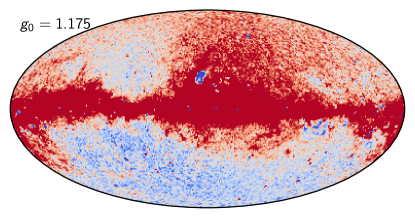
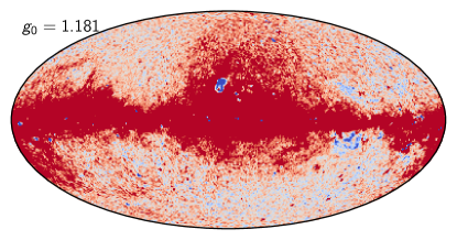
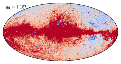
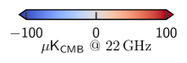
Figure 2: Dependence of AME amplitude evaluated at 22 GHz on the absolute calibration. Each map comes from the fifth iteration of a dedicated Commander3 run that fixed $g_{0}$ while letting all other TOD parameters be fit. The values of $g_{0}=1.175$ and $g_{0}=1.187$ represent $6\sigma$ draws from the prior distribution with mean $1.181$ and standard deviation $0.001$. Extreme outliers were chosen to illustrate this effect. The dipole visible in the top and bottom panels is aligned perfectly with the Solar dipole, and is directly due to variations in the K-band absolute calibration.

The model described in Sects. 2.2 and 2.3 is prone to several degeneracies, allowing for unphysical solutions to be explored in the Gibbs chain. Such unphysical degeneracies are highly undesirable for two main reasons. First, they increase the statistical uncertainties on most (if not all) other important parameters in the model – sometimes to the point that the target quantity is rendered entirely unmeasurable. Secondly, and perhaps even more importantly, the data model described above is known to be a (sometimes crude) approximation to the real observations, and there will invariably be modeling errors. Degeneracies tend to amplify their impact, in the sense that any unconstrained parameters will typically be used to fit such small modeling errors. For both these reasons, it is preferable to impose either informative or algorithmic priors on the unconstrained parameters, rather than to leave them entirely unconstrained in the model.

An important example of an algorithmic prior is the foreground smoothing prior used by Planck Collaboration IV (2018) and Andersen et al. (2023), which dictates that astrophysical foregrounds must be smooth on small angular scales. This is justified by noting that the angular spectrum on large and intermediate scales typically falls as a power-law in multipole space; extrapolating this into the noise dominated regime prevents the overall foreground model from becoming degenerate at small scales.

Correspondingly, important examples of informative priors are the use of HFI constraints on the thermal dust SED parameters, $\beta_{\mathrm{d}}$ and $T_{\mathrm{d}}$ in BeyondPlanck. Because that analysis only included the highest HFI frequency channel, they had very little constraining power on the thermal dust SED. Rather than trying to fit these directly from LFI WMAP alone, they instead imposed informative Gaussian priors on each of these parameters, as derived from the HFI observations (Planck Collaboration IV 2018).

Unless otherwise noted, we adopt the same algorithmic and informative priors as BeyondPlanck (2023). However, there are three notable exceptions, as detailed below. All of these are dictated either by the fact that we include the WMAP K-band channel (which has a strong impact on the low-frequency foreground model), or by the fact that we now process the WMAP data in the time domain, and therefore are subject to the same degeneracies as the official WMAP low-level pipeline; degeneracies that were solved with either implicit or explicit priors in the original analysis.

First and foremost, and discussed further in Sect. 7.3, we observe a very strong degeneracy between the absolute calibration of the K-band channel and the dipole of the AME map. This is not unexpected, considering K-band is by far the strongest channel in terms of AME signal-to-noise ratio, exceeding that of LFI 30 GHz by about 50 % (see Sect. 6.4 for details). Effectively, a small variation in the absolute gain may be countered by subtracting the corresponding CMB Solar dipole variation from the AME map, and end up with a nearly identical total $\chi^{2}$; the orbital CMB dipole is not bright enough at 23 GHz relative to AME emission to break this degeneracy on its own.

This is illustrated in Fig. 2, which shows the AME amplitude map as derived for three different values of the mean K-band gain, $g_{0}$, namely 1.175, 1.181, and $1.184\thinspace\mathrm{du\thinspace mK^{-1}}$; the extreme values differ only by 0.5 %. All of these three values appear equally acceptable from a pure $\chi^{2}$ point-of-view, relative to the noise level and modeling errors of these data. At the same time, it is clear from visual inspection that only the middle value actually makes physical sense, given what we know about the structure of the Milky Way. For this reason, we apply a Gaussian prior on the absolute K-band gain of $g_{0}\sim\mathcal{N}(1.181,0.001^{2})$ to regularize this issue. Thus, the extreme panels in Fig. 2 represent $\pm 6\thinspace\sigma$ outliers, respectively, and will appear in our Markov chains with a frequency of about 1-in-$10^{9}$.

It is reasonable to ask why the WMAP pipeline produced sensible results without applying such a prior during their calibration procedure. We posit that the answer is due to the main difference between the two approaches. While Cosmoglobe attempts to fit a single overall parametric model to all data at once, the WMAP pipeline calibrated each channel independently by co-adding data from one channel into a map, subtracting that map from the TOD, fitting the gain to the orbital dipole, and iterating until the solution became stable. An advantage of the single-channel approach is that the solution is independent of the assumed sky model. However, a disadvantage is that it is impossible to break any potential inherent degeneracies; it cannot be combined with external observations in any meaningful way. One important example of this regarding the WMAP data is a strong degeneracy between the transmission imbalance factors and the polarized sky signal; it is exceedingly difficult to break this degeneracy using data from only one DA alone, and the resulting errors will propagate to most other aspects in the analysis. In the global approach, on the other hand, the polarization modes that are poorly measured by WMAP alone are well measured by Planck and vice-versa, resulting in an overall better constrained fit.

Second, as reported by Svalheim et al. (2023b) for the BeyondPlanck analysis, another important degeneracy in the current global model concerns the spectral index of polarized synchrotron emission versus the time-variable detector gain; when fitting both the polarized synchrotron amplitude and calibration freely without priors, the synchrotron spectral index at high Galactic latitudes tend to be biased toward unreasonably flat values, $\beta_{\mathrm{s}}\lesssim-2.5$, which was likely due to a low level of unmodeled systematics, for instance temperature-to-polarization leakage, rather than true polarized synchrotron emission. In turn, this resulted in a contaminated CMB sky map with a strong synchrotron morphology. To break this degeneracy, Svalheim et al. (2023b) chose to marginalize the high-latitude synchrotron spectral index over a Gaussian prior of $\mathcal{N}(-3.30,0.1^{2})$, informed by Planck Collaboration V (2020), rather than estimate it from the data themselves. We observe the same degeneracy, and the introduction of the K-band data is not sufficient to break it on its own. For this reason, we choose to apply the same informative prior.

Third and finally, we also marginalize over the AME scale index with a prior of $\beta_{\mathrm{AME}}\sim\mathcal{N}(3.56,0.1^{2})$. The parameters of these priors were determined by running a grid over $\beta_{\mathrm{AME}}$, and identifying the range that resulted in reasonable residuals near the Galactic plane, similar to that shown in Fig. 2 for the absolute calibration of K-band. We note that this prior should in principle be replaced with direct $\chi^{2}$-based posterior optimization, combined with a properly tailored analysis mask. However, the recent release of the QUIJOTE data (Rubiño-Martín et al. 2023), which covers the 11–19 GHz frequency range, suggests that the entire AME model should be revisited in a future joint WMAP+LFI+QUIJOTE analysis. We therefore leave detailed prior and SED optimization to that work. For further information regarding AME modeling with the current dataset, we refer the interested reader to Watts et al. (2023a).

In sum, we impose strong priors on all foreground spectral indices, with parameters that are informed by the requirement of obtaining physically meaningful component maps. These strong priors imply that the foreground spectral parameters sampled within the chain do not carry independent significance in the traditional posterior sense, but are in practice only nuisance parameters used to marginalize over externally defined uncertainties.

2.5 Posterior distribution and Gibbs sampling

As shown by BeyondPlanck (2023), this joint parametric description of the instrumental effects and sky allows us to write down a total model for the data, $\boldsymbol{d}=\boldsymbol{s}^{\mathrm{tot}}(\boldsymbol{\omega})+\boldsymbol{n}^{\mathrm{w}}$, where $\boldsymbol{s}^{\mathrm{tot}}$ encompasses all of the terms in Eq. (6) except for the white noise term. Assuming that all instrumental effects have been modeled adequately, and that the white noise is Gaussian distributed, the data should then also be Gaussian distributed with a mean of $\boldsymbol{s}^{\mathrm{tot}}(\boldsymbol{\omega})$ and variance $\boldsymbol{\sigma}_{0}^{2}$. In general, the likelihood reads

$$P(\boldsymbol{d}\mid\boldsymbol{\omega})\propto\exp\left(-\frac{1}{2}\sum_{t}\frac{(d_{t}-s^{\mathrm{tot}}_{t}(\boldsymbol{\omega}))^{2}}{\sigma_{0}^{2}}\right).$$ (16)

If $\boldsymbol{d}\sim\mathcal{N}(\boldsymbol{s}^{\mathrm{tot}},\boldsymbol{\sigma}_{0}^{2})$ is the correct model for the data, the argument of the exponent is proportional to a $\chi^{2}$-distribution with $n_{\mathrm{TOD}}$ degrees of freedom, where $n_{\mathrm{TOD}}$ number of datapoints within a given datastream. In the limit of large $n$, a $\chi^{2}$ distribution is well-approximated by a Gaussian with mean $n$ and variance $2n$. Therefore we define and use the reduced normalized $\chi^{2}$ statistic,

$$\chi^{2}\equiv\frac{\sum_{t}((d_{t}-s_{t}^{\mathrm{tot}})/\sigma_{0})^{2}-n_{\mathrm{TOD}}}{\sqrt{2n_{\mathrm{TOD}}}},$$ (17)

which is approximately drawn from the standard normal distribution $\mathcal{N}(0,1)$.

Following BeyondPlanck (2023), the Cosmoglobe Gibbs chain for this analysis is given by

$$\boldsymbol{s}^{\mathrm{inst}} \thinspace\leftarrow P(\boldsymbol{s}^{\mathrm{inst}} \thinspace\mid\@vec{d}, \thinspace\@vec{g}, \thinspace\boldsymbol{x}_{\mathrm{im}}, \thinspace\@vec{n}^{\mathrm{corr}}, \thinspace\boldsymbol{\xi}_{n}, \thinspace\boldsymbol{\beta}, \thinspace\boldsymbol{a}, \thinspace C_{\ell})$$ (18)

$$\@vec{g} \thinspace\leftarrow P(\@vec{g} \thinspace\mid\@vec{d}, \thinspace\boldsymbol{s}^{\mathrm{inst}}, \thinspace\boldsymbol{x}_{\mathrm{im}}, \thinspace\@vec{n}^{\mathrm{corr}}, \thinspace\boldsymbol{\xi}_{n}, \thinspace\boldsymbol{\beta}, \thinspace\boldsymbol{a}, \thinspace C_{\ell})$$ (19)

$$\boldsymbol{x}_{\mathrm{im}} \thinspace\leftarrow P(\boldsymbol{x}_{\mathrm{im}} \thinspace\mid\@vec{d}, \thinspace\boldsymbol{s}^{\mathrm{inst}}, \thinspace\@vec{g}, \thinspace\@vec{n}^{\mathrm{corr}}, \thinspace\boldsymbol{\xi}_{n}, \thinspace\boldsymbol{\beta}, \thinspace\boldsymbol{a}, \thinspace C_{\ell})$$ (20)

$$\@vec{n}^{\mathrm{corr}} \thinspace\leftarrow P(\@vec{n}^{\mathrm{corr}} \thinspace\mid\@vec{d}, \thinspace\boldsymbol{s}^{\mathrm{inst}}, \thinspace\@vec{g}, \thinspace\boldsymbol{x}_{\mathrm{im}}, \thinspace\boldsymbol{\xi}_{n}, \thinspace\boldsymbol{\beta}, \thinspace\boldsymbol{a}, \thinspace C_{\ell})$$ (21)

$$\boldsymbol{\xi}_{n} \thinspace\leftarrow P(\boldsymbol{\xi}_{n} \thinspace\mid\@vec{d}, \thinspace\boldsymbol{s}^{\mathrm{inst}}, \thinspace\@vec{g}, \thinspace\boldsymbol{x}_{\mathrm{im}}, \thinspace\@vec{n}^{\mathrm{corr}}, \thinspace\boldsymbol{\beta}, \thinspace\boldsymbol{a}, \thinspace C_{\ell})$$ (22)

$$\boldsymbol{\beta} \thinspace\leftarrow P(\boldsymbol{\beta})$$ (23)

$$\boldsymbol{a} \thinspace\leftarrow P(\boldsymbol{a} \thinspace\mid\@vec{d}, \thinspace\boldsymbol{s}^{\mathrm{inst}}, \thinspace\@vec{g}, \thinspace\boldsymbol{x}_{\mathrm{im}}, \thinspace\@vec{n}^{\mathrm{corr}}, \thinspace\boldsymbol{\xi}_{n}, \thinspace\boldsymbol{\beta}, \thinspace C_{\ell})$$ (24)

$$C_{\ell} \thinspace\leftarrow P(C_{\ell} \thinspace\mid\boldsymbol{a})$$ (25)

with each step requiring its own dedicated sampling algorithm. The Commander3 pipeline is designed so that results of each Gibbs sample can be easily passed to each other, and that the internal calculations of each step do not directly depend on the inner workings of each other, which greatly increases modularity of the code.

2.6 Sampling algorithms

Before we discuss the results of this Gibbs chain as applied to the Planck LFI and WMAP data, we summarize the TOD processing steps in this section. Each step of the Gibbs chain requires its own conditional distribution sampling algorithm. In Sect. 2.6.1 we review the sampling algorithms implemented in the BeyondPlanck suite of papers, while Sects. 2.6.2–2.6.3 provide an overview of the WMAP-specific processing steps.

2.6.1 Review of sampling algorithms

Most of the techniques required for WMAP data analysis have already been described in the BeyondPlanck project and implemented in Commander3. This section includes a summary of the algorithms that were used previously for the analysis of LFI data. In each of these cases, every part of the model not explicitly mentioned is held fixed unless specified otherwise.

Noise estimation and calibration are described by Ihle et al. (2023) and Gjerløw et al. (2023), respectively. As noted in those works, these two steps are strongly correlated, simply because the timestream

$$\boldsymbol{d}_{i}=\boldsymbol{g}_{i}\boldsymbol{s}_{i}^{\mathrm{tot}}+\boldsymbol{n}_{i}^{\mathrm{corr}}+\boldsymbol{n}_{i}^{\mathrm{w}}$$ (26)

may be almost equally well fit by two solutions defined schematically by

$$\boldsymbol{g}^{\prime}=\boldsymbol{g}\boldsymbol{s}^{\mathrm{tot}}/(\boldsymbol{s}^{\mathrm{tot}})^{\prime}$$ (27)

or

$${(\boldsymbol{n}^{\mathrm{corr}})^{\prime}=\boldsymbol{n}^{\mathrm{corr}}+\boldsymbol{g}\boldsymbol{s}^{\mathrm{tot}}+\boldsymbol{g}^{\prime}(\boldsymbol{s}^{\mathrm{tot}})^{\prime}};$$ (28)

the only thing that breaks this degeneracy is the noise PSD, which is a relatively loose constraint. A Gibbs sampler is not very effective for nearly degenerate distributions, and we therefore instead define a joint sampling step for the correlated noise and gain. In practice, this is done by first drawing the calibration from its marginal distribution with respect to $\boldsymbol{n}^{\mathrm{corr}}$, and then drawing $\boldsymbol{n}^{\mathrm{corr}}$ from its conditional distribution with respect to $\boldsymbol{g}$,

$$\@vec{g} \thinspace\leftarrow P(\@vec{g} \thinspace\mid\@vec{d}, \thinspace\boldsymbol{\xi}_{n})$$ (29)

$$\@vec{n}^{\mathrm{corr}} \thinspace\leftarrow P(\@vec{n}^{\mathrm{corr}} \thinspace\mid\@vec{d}, \thinspace\@vec{g}, \thinspace\boldsymbol{\xi}_{n}).$$ (30)

One can see that this is a valid sample from the joint distribution from the definition of a conditional distribution, $P(\@vec{g},\@vec{n}^{\mathrm{corr}}\mid\boldsymbol{\omega})=P(\@vec{n}^{\mathrm{corr}}\mid\@vec{g},\boldsymbol{\omega})P(\@vec{g}\mid\boldsymbol{\omega})$. In practice, this simply means that when sampling for $\@vec{g}$, the covariance matrix $\mathsf{N}=\mathsf{N}_{\textrm{w}}+\mathsf{N}_{\textrm{corr}}$ must be used, rather than just $\mathsf{N}_{\mathrm{w}}$.

Commander3 models the gain at each timestream $t$ for a detector $i$ as

$$g_{t,i}=g_{0}+\Delta g_{i}+\delta g_{q,i},$$ (31)

where $q$ labels the time interval for which we assume the gain is constant, typically a single scan. In order to sample the gain, we write down a generative model for the TOD,

$$\@vec{d}_{i}=\@vec{g}_{i}\@vec{s}_{i}^{\mathrm{tot}}+\@vec{n}_{i}^{\mathrm{tot}}\sim\mathcal{N}(\@vec{g}_{i}\@vec{s}_{i}^{\mathrm{tot}},\mathsf{N}_{i}).$$ (32)

Since $\@vec{d}_{i}$ is given as a linear combination of the fixed signal and the gains, a random sample of the gain can be drawn by solving

$$[(\@vec{s}_{i}^{\mathrm{tot}})^{T}\mathsf{N}_{i}^{-1}\@vec{s}_{i}^{\mathrm{tot}}]\@vec{g}_{i}=(\@vec{s}_{i}^{\mathrm{tot}})^{T}\@tens{N}^{-1}_{i}\@vec{d}_{i}+(\@vec{s}_{i}^{\mathrm{tot}})^{T}\@tens{N}^{-1/2}_{i}\boldsymbol{\eta},$$ (33)

where $\boldsymbol{\eta}\sim\mathcal{N}(0,1)$ is a vector of standard normal variables. Note that $\mathsf{N}_{i}$ depends implicitly on the noise PSD $\boldsymbol{\xi}_{n}$, while the fluctuations corresponding to $\@vec{n}^{\mathrm{corr}}$ are properly downweighted by $\mathsf{N}_{\mathrm{corr},i}$. As detailed by Gjerløw et al. (2023), Commander3 samples $g_{0}$, $\Delta g_{i}$, and $\delta g_{q,i}$ in separate steps. Specifically, the absolute calibration $g_{0}$, for the CMB-dominated channels, is fitted using only the orbital dipole, while the relative calibrations, $\Delta g_{i}$, exploits the full sky signal. The same is true for the time-dependent gain fluctuations, $\delta g_{q,i}$, and in this case an additional smoothness prior is applied through an effective Wiener filter. The Gibbs chain is formally broken by fitting the absolute gain $g_{0}$ to the orbital dipole alone, as opposed to the full sky signal. However, this makes the sampling more robust with respect to unmodeled systematic effects, somewhat analogous to applying a confidence mask when estimating the CMB power spectrum.

The correlated noise sampling, described by Ihle et al. (2023), follows a similar procedure, except this now conditions upon the previous gain estimate, which is sampled immediately before the correlated noise component in the code. Similar to the gain case, we can write a generative model for the data,

$$\@vec{d}_{i}=\@vec{g}_{i}\@vec{s}_{i}^{\mathrm{tot}}+\@vec{n}_{i}^{\mathrm{corr}}+\@vec{n}^{\mathrm{w}}_{i}\sim\mathcal{N}(\@vec{g}_{i}\@vec{s}_{i}^{\mathrm{tot}},\@tens{N}_{\mathrm{corr},i}+\@tens{N}_{\mathrm{w},i}).$$ (34)

Given fixed $\boldsymbol{r}_{i}=\@vec{d}_{i}-\@vec{g}_{i}\@vec{s}_{i}^{\mathrm{tot}}$, we can again write a sampling equation,

$$(\@tens{N}_{\mathrm{corr},i}^{-1}+\@tens{N}_{\mathrm{w},i}^{-1})\@vec{n}^{\mathrm{corr}}_{i}=\@tens{N}^{-1}_{\mathrm{w},i}\boldsymbol{r}_{i}+\@tens{N}^{-1/2}_{\mathrm{w},i}\boldsymbol{\eta}_{1}+\@tens{N}^{-1/2}_{\mathrm{corr},i}\boldsymbol{\eta}_{2}.$$ (35)

This gives a sample of the underlying correlated noise.

To sample the correlated noise parameters, we assume that the correlated noise is drawn from a correlated Gaussian and from the conditional posterior distribution,

$$P(\boldsymbol{\xi}_{n}\mid\@vec{n}^{\mathrm{corr}})\propto\frac{\exp{[-\frac{1}{2}(\@vec{n}^{\mathrm{corr}})^{T}\@tens{N}_{\mathrm{corr}}^{-1}\@vec{n}^{\mathrm{corr}}]}}{\sqrt{|\@tens{N}_{\mathrm{corr}}|}}P(\boldsymbol{\xi}_{n}).$$ (36)

where $P(\boldsymbol{\xi}_{n})$ is a flat prior over the PSD parameters. The simplest and most commonly used parametrization for correlated noise is given by

$$\mathsf{N}_{\mathrm{corr}}(f)=\sigma_{0}^{2}\left(\frac{f}{f_{\mathrm{knee}}}\right)^{\alpha}.$$ (37)

This can in principal be modified, and for Planck LFI a Gaussian log-normal bump was added at a late stage in the BeyondPlanck analysis. Rather than sampling for $\sigma_{0}$, we effectively fix the white noise level to the noise level at the highest frequency, e.g.,

$$\sigma_{0}^{2}\equiv\frac{\mathrm{Var}(r_{t+1}-r_{t})}{2},$$ (38)

where $t$ and $t+1$ are consecutive time samples, and ${\boldsymbol{r}\equiv\boldsymbol{d}-\boldsymbol{g}\boldsymbol{s}^{\mathrm{tot}}-\boldsymbol{n}^{\mathrm{corr}}}$. In practice, this makes $\sigma_{0}$ a deterministic function of the sampled sky and gain parameters. The parameters $\alpha$ and $f_{\mathrm{knee}}$ are not linear in the data, but they can be sampled efficiently using a standard inversion sampler (see, e.g., Appendix A.3 of BeyondPlanck 2023 or Chapter 7.3.2 of Press et al. 2007 for further details). In practice, this requires computing the posterior over a linear grid one parameter at a time.

Once the instrumental parameters have been sampled, Commander3 computes the calibrated TOD for each band,

$$r_{t,i}=\frac{d_{t,i}-n_{t,i}^{\mathrm{corr}}}{g_{t,i}}-\left(s_{t,i}^{\mathrm{orb}}+s_{t,i}^{\mathrm{fsl}}+\delta s_{t,i}^{\mathrm{leak}}+{s}_{t,i}^{\mathrm{inst}}\right)$$ (39)

where $\@vec{s}^{\mathrm{orb}}$ is the orbital dipole (Gjerløw et al. 2023), $\@vec{s}^{\mathrm{fsl}}$ is the far sidelobe timestream (Galloway et al. 2023b), $\delta\@vec{s}^{\mathrm{leak}}$ is the bandpass leakage (Svalheim et al. 2023a), and $\@vec{s}^{\mathrm{inst}}$ is some instrumental-specific contribution, e.g., the 1 Hz electronic spike for LFI. With a correlated noise realization removed, one can perform simple binned mapmaking, weighting each pixel by the white noise amplitude.

2.6.2 Differential mapmaking

The first additional algorithm that needs to be added to Commander3 in order to process WMAP TOD data is support for differential mapmaking (Watts et al. 2023b). After calibration and correction for instrumental effects, the TOD can be modeled as

$$\boldsymbol{d}=\mathsf{P}\boldsymbol{m}+\boldsymbol{n}^{\mathrm{w}},$$ (40)

where

$$\boldsymbol{m}=\mathsf{B}^{\mathrm{symm}}\mathsf{M}\boldsymbol{a}$$ (41)

is the expected map for each detector after removing the orbital dipole, far sidelobe, baseline, and a realization of correlated noise. The differential pointing strategy can be represented in matrix form as

$$\mathsf{P}_{tp} =(1+x_{\mathrm{im}})(\delta_{p^{I}_{\phantom{\mathrm{A}}}p_{\mathrm{A}}^{I}}+\delta_{p^{Q}_{\phantom{\mathrm{A}}}p^{Q}_{\mathrm{A}}}\cos 2\psi_{\mathrm{A}}+\delta_{p^{U}_{\phantom{\mathrm{A}}}p^{U}_{\mathrm{A}}}\sin 2\psi_{\mathrm{A}})$$ (42)

$$-(1-x_{\mathrm{im}})(\delta_{p^{I}_{\phantom{\mathrm{B}}}p_{\mathrm{B}}^{I}}-\delta_{p^{Q}_{\phantom{\mathrm{A}}}p^{Q}_{\mathrm{B}}}\cos 2\psi_{\mathrm{B}}-\delta_{p^{U}_{\phantom{\mathrm{A}}}p^{U}_{\mathrm{B}}}\sin 2\psi_{\mathrm{B}})$$

where $p_{\mathrm{A}}$ and $p_{\mathrm{B}}$ are the time-dependent pointings for each DA. Note that this is equivalent to Eqs. (4) and (5), except without the spurious component $S_{\mathrm{A}/\mathrm{B}}$ as the bandpass mismatch is explicitly subtracted beforehand in Eq. (39). The maximum likelihood map can now in principle be derived using the usual mapmaking equation,

$$\mathsf{P}^{T}\mathsf{N}^{-1}\mathsf{P}\boldsymbol{m}=\mathsf{P}^{T}\mathsf{N}^{-1}\boldsymbol{d}.$$ (43)

For a single-horn experiment, i.e., Planck LFI, this reduces to a $3\times 3$ matrix that can be inverted for each pixel independently. For the pointing matrix in Eq. (42), this is no longer possible, as there is inherently coupling between horns A and B in the timestreams. The $3N_{\mathrm{pix}}\times 3N_{\mathrm{pix}}$ matrix can in principle be solved using an iterative algorithm, e.g., preconditioned conjugate gradients (Shewchuk 1994).

Jarosik et al. (2011) identified an issue where a large difference in the sky temperature values at pixel A versus pixel B induced artifacts in the mapmaking procedure. We adopt the procedure first described by Hinshaw et al. (2003) where only the pixel in a bright region, defined by a small processing mask (Bennett et al. 2013) is accumulated, thus modifying the mapmaking equation to

$$\mathsf{P}^{T}_{\mathrm{am}}\mathsf{N}^{-1}\mathsf{P}\boldsymbol{m}=\mathsf{P}^{T}_{\mathrm{am}}\mathsf{N}^{-1}\boldsymbol{d}.$$ (44)

This equation can be solved using the BiCG-STAB algorithm for a non-symmetric matrix $\mathsf{A}$ where $\mathsf{A}\boldsymbol{x}=\boldsymbol{b}$. We apply a preconditioner $\mathsf{M}$ by numerically inverting the same problem with $N_{\mathrm{side}}=16$ maps and applying a diagonal noise matrix. Numerically, we define convergence as when the residual $\boldsymbol{r}\equiv\boldsymbol{b}-\mathsf{A}\boldsymbol{x}$ satisfies $\boldsymbol{r}^{T}\mathsf{M}^{-1}\boldsymbol{r}/\boldsymbol{b}^{T}\mathsf{M}^{-1}\boldsymbol{b}<10^{-10}$, which typically takes about 20 iterations for producing frequency maps.

The full noise covariance matrix $\mathsf{N}_{pp^{\prime}}$ is given by the inverse of $\mathsf{P}^{T}_{\mathrm{am}}\mathsf{N}^{-1}\mathsf{P}$, where the diagonals $\mathsf{N}_{pp}$ are the white noise variance for each Stokes parameter. An additional quantity that was computed in BeyondPlanck but not delivered in the final products is the covariance of the Stokes parameters within a single pixel, $\sigma_{QU,p}$. We find that the correlation between Stokes parameters, $\rho_{QU}\equiv\sigma_{QU}/\sqrt{\sigma_{QQ}\sigma_{UU}}$, is of order 0.5 for the WMAP DAs, as shown in Fig. 3. For Planck LFI, the 30 and 70 GHz channels have $|\rho_{QU}|\sim 0.1$, while the 44 GHz correlations are notably higher with $|\rho_{QU}|\sim 0.5$. The reason for this difference is that the 44 GHz channel has three horns. Two of those are aligned with the scanning direction in the focal plane, and have polarization angles that are rotated by $45^{\circ}$ with respect to each other. Together those two horns therefore disentangle polarization information very efficiently. The third horn, however, does not have a corresponding partner, and relies only on satellite precession to recover individual Stokes parameters. For comparison, all 30 and 70 GHz horns have partners aligned with the scanning direction. In the current work, we have implemented support for the full $3\times 3$ noise matrices, including $\sigma_{QU},$ for component separation and map-based $\chi^{2}$ calculations for both WMAP and LFI.

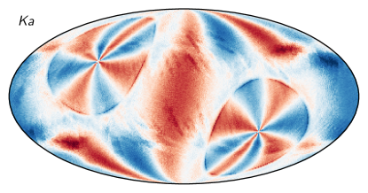
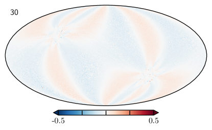
Figure 3: Cross-correlation $\rho_{QU}$ per pixel for (top:) Ka and (bottom:) LFI 30 GHz.

2.6.3 Baseline sampling

The data model adopted by Hinshaw et al. (2003) can be written in raw du as

$$\@vec{d}=\mathsf{GPBM}\boldsymbol{a}+\boldsymbol{n}+\boldsymbol{b},$$ (45)

where $\boldsymbol{b}$ is the instrumental baseline and $\boldsymbol{n}$ is the total instrumental noise. As noted above, Commander3 divides the noise into $\@vec{n}=\@vec{n}^{\mathrm{w}}+\@vec{n}^{\mathrm{corr}}$, a white noise term and a correlated noise term. Because the white noise is by definition uncorrelated in time, it does not have any correlations between adjacent pixels, so that any pixel-pixel covariance should be fully described by realizations of the $\@vec{n}^{\mathrm{corr}}$ timestream.

Commander3 estimates the baseline using the full estimate of the current sky model, $\boldsymbol{r}=\boldsymbol{d}-\boldsymbol{g}\boldsymbol{s}^{\mathrm{tot}}=\boldsymbol{b}+\boldsymbol{n}$. Modeling $\boldsymbol{b}=b_{0}+b_{1}\Delta t$, we solve for $b_{0}$ and $b_{1}$ using linear regression in each timestream while masking out samples that lie within the processing mask. Strictly speaking, this is breaking the Gibbs chain, as we are not formally sampling $b_{0}$ and $b_{1}$ for each TOD chunk. In practice, baseline estimation uncertainty propagates to correlated noise realizations and PSD parameters, as discussed below.

The approach detailed by Hinshaw et al. (2003) and the Commander3 implementation differ mainly in two ways. First, the assumed stable timescales are different – the initial WMAP baseline is estimated over one hour timescales, and assumed to be an actual constant, whereas Commander3 assumes constant values through the entire time chunk, which is 3–7 days depending on the band in question, but allows a linear term in the baseline. Second, the two methods differ in how they treat nonlinear residuals in the first-order baseline model. As noted by Hinshaw et al. (2003), residual baseline variations manifest as correlated noise stripes in the final maps, and WMAP9 solves this using a time domain filter, downweighting the data based on the noise characterization. This is similar to the Commander3 approach, which accounts for this as part of the correlated noise component. The main advantages of the latter is that it allows for proper error propagation at all angular scales without the use of a dense pixel-pixel noise covariance, and provides a convenient means for inspecting the residuals visually by binning the correlated noise into a sky map.

2.6.4 Transmission imbalance estimation

Transmission imbalance, the differential power transmission of the optics and waveguide components between horns A and B, can be parameterized as

$$d_{t,i}=g_{t,i}[(1+x_{\mathrm{im},i})s_{t,i}^{\mathrm{tot,A}}-(1-x_{\mathrm{im},i})s_{t,i}^{\mathrm{tot,B}}]+n_{t}.$$ (46)

This can be decomposed into a differential (d) and common-mode (c) signal such that

$$d_{t,i}=g_{t,i}[s_{t,i}^{\mathrm{d}}+x_{\mathrm{im},i}s_{t,i}^{\mathrm{c}}]+n_{t}.$$ (47)

In this form, the imbalance parameters can be estimated by drawing Gaussian samples from the standard mean and standard deviation over the entire mission. To draw samples for $x_{\mathrm{im},i}$, we construct a sampling routine analogous to the gain estimation of Eq. (33) and correlated noise estimation of Eq. (35), with $\boldsymbol{r}=\boldsymbol{d}-\boldsymbol{g}\boldsymbol{s}^{\mathrm{d}}$,

$$[(\boldsymbol{g}\boldsymbol{s}^{\mathrm{c}})^{T}\mathsf{N}^{-1}\boldsymbol{g}\boldsymbol{s}^{\mathrm{c}}]x_{\mathrm{im}}=(\boldsymbol{g}\boldsymbol{s}^{\mathrm{c}})^{T}\mathsf{N}^{-1}\boldsymbol{r}+(\boldsymbol{g}\boldsymbol{s}^{\mathrm{c}})^{T}\mathsf{N}^{-1/2}\boldsymbol{\eta},$$ (48)

cross-correlating the common-mode signal with $\boldsymbol{r}$ with appropriate weights and adding a Gaussian random variable with the correct weighting. Note that we are marginalizing over the correlated noise here by using $\@tens{N}=\@tens{N}_{\mathrm{w}}+\@tens{N}_{\mathrm{corr}}$. This mitigates any baseline drifts being erroneously attributed to the common-mode signal and biasing the estimate of $x_{\mathrm{im}}$.

The WMAP procedure, described by Jarosik et al. (2003a), fit for common-mode and differential coefficients along with a cubic baseline over 10 precession periods at a time, corresponding to 10 hours of observation. The mean and uncertainty were then calculated by averaging and taking the standard deviation of these values. This approach has the benefit of allowing for the tracking of possible transmission imbalance variation throughout the mission. However, none of the WMAP suite of papers have found evidence for this, and it has not arisen in our analysis, so we model this as an effect whose value is constant throughout the mission.

3 Data and data processing

Table 1: Cosmoglobe flagging statistics for each DA. The second column indicates the fraction of data that are removed by the official WMAP flags, while the third column indicates the fraction that is additionally discarded in the current processing for computational reasons. The fourth column indicates the total fraction of data actually used to generate the final maps.

Band	Flagged (%)	Discarded (%)	Used (%)
K	1.72	0.87	97.4
Ka	1.64	0.88	97.5
Q1	1.84	0.84	96.5
Q2	1.62	0.81	97.6
V1	1.62	1.10	97.3
V2	1.61	1.01	97.4
W1	1.76	1.03	97.2
W2	1.60	0.81	97.6
W3	1.61	0.87	97.5
W4	1.60	0.81	97.6

Table 2: Computational resources required for end-to-end Cosmoglobe processing. All times correspond to CPU hours, and all data volumes are reported in GB. Reported times are averaged over more than 100 samples, and vary by $\lesssim\thinspace 5\thinspace\%$ from sample to sample. Note that the average cost per sample takes into account the undersampling of 70, V, and W.

Item 30 44 70 K Ka Q1 Q2 V1 V2 W1 W2 W3 W4 Sum Data volume    Compressed TOD volume . 86 178 597 13 12 15 15 19 18 26 26 26 26 1 053 Processing time (cost per run)    TOD initialization/IO time . 1.8 2.5 7.8 0.7 0.6 0.8 0.7 0.9 0.8 1.3 1.3 1.0 0.9 21.1    Other initialization . 14.6    Total initialization . 35.7 Gibbs sampling steps (cost per sample)    Huffman decompression . 1.2 2.2 23.2 0.8 0.9 1.1 1.1 1.5 1.4 2.0 2.0 2.0 2.0 41.4    Array allocation . 0.4 0.9 51.6 1.3 1.3 1.5 1.5 3.1 3.3 4.0 3.8 4.0 4.0 80.7    TOD projection ($$\@tens{P} \@tens{P}^{t}$$ operation) . 0.9 2.0 12.3 6.1 7.1 8.7 8.9 11.4 11.3 15.9 15.8 15.7 15.8 131.9    Sidelobe evaluation . 1.2 2.6 9.5 3.0 3.5 4.1 4.2 5.5 5.4 7.8 7.7 7.7 7.5 69.7    Orbital dipole . 0.9 2.0 9.0 1.2 1.5 1.8 1.9 2.6 2.5 3.8 3.8 3.8 3.8 38.6    Gain sampling . 0.6 0.9 2.2 1.3 1.3 0.8 0.8 1.3 1.3 1.2 1.2 1.2 1.2 15.3    1 Hz spike sampling . 0.3 0.4 1.9 2.7    Correlated noise sampling . 2.1 4.3 24.8 2.7 2.9 3.7 3.8 6.2 5.4 7.7 7.4 6.9 8.3 86.4    Correlated noise PSD sampling . 5.0 6.2 1.6 0.3 0.3 0.3 0.3 0.5 0.5 0.7 0.6 0.6 0.7 17.6    TOD binning ( operation) . 0.1 0.1 10.5 0.8 0.8 1.0 1.0 1.7 1.6 2.4 2.4 2.4 2.4 27.2    Mapmaking . 9.2 9.7 13.1 12.7 21.7 20.2 35.4 34.9 36.1 39.3 232.3    MPI load-balancing . 1.2 1.7 9.2 2.2 2.0 2.2 2.1 3.6 3.3 4.8 4.6 4.5 4.6 46.0    Sum of other TOD processing . 0.7 1.6 13.1 0.1 0.2 0.5 0.4 0.7 0.8 0.9 1.0 0.9 1.2 22.1    TOD processing cost per sample . 14.6 24.9 169.7 28.8 31.5 38.7 38.7 59.8 57.0 86.6 85.2 85.8 90.8 812.1    Amplitude sampling . 16.2    Spectral index sampling . 32.1    Average cost per sample . 418.9

We describe the public WMAP9 data products in Sect. 3.1, then describe the treatment we apply to make them compatible with Commander3 in Sect. 3.2. Finally, we describe the computational requirements in Sect. 3.3.

3.1 Publicly available WMAP products

The full WMAP dataset is hosted at the Legacy Archive for Microwave Background Data Analysis (LAMBDA). In addition to the primary scientific products, e.g., cosmological parameters, CMB power spectra and anisotropy maps and frequency maps, the time-ordered data (TOD) can be downloaded, both in uncalibrated and calibrated form. In principle, thanks to these data and the explanatory supplements (Greason et al. 2012), the entire data analysis pipeline can be reproduced from uncalibrated TOD to frequency maps.

For this analysis, we keep certain instrumental parameters fixed to the reported values. For example, we have made no attempts to rederive the pointing solutions, re-estimate the main beam response and far sidelobe pickup, or recover data that were flagged in the WMAP event log. These and other analyses, such as estimating the bandpass shift over the course of the mission, are certainly possible within the larger Gibbs sampling framework. However, in this work we limit ourselves to recalibrating the TOD, estimating their noise properties, and applying bandpass corrections to the data before mapmaking.

3.2 TOD preprocessing and data selection

The full nine-year WMAP archive spans from 10 August 2001 to 10 August 2010, with the raw uncalibrated data comprising 626 GB. A little over 1 % of the data were lost or rejected due to incomplete satellite telemetry, thermal disturbances, spacecraft anomalies, and station-keeping maneuvers, with an extra 0.1 % rejected due to planet flagging (Bennett et al. 2003b; Hinshaw et al. 2007, 2009; Bennett et al. 2013). The final results reported by Bennett et al. (2013) included roughly 98.4 % of the total data volume. A full accounting of all data cuts can be found in Table 1.8 of Greason et al. (2012). In this analysis we flag the same data indicated in the fiducial WMAP analysis, and use the same planet exclusion radii.

As shown by Galloway et al. (2023a), a large fraction of Commander3’s computational time is spent performing Fast Fourier Transforms (FFTs) on individual scans. Rather than truncating datastreams to have lengths equal to “magic numbers” for which FFTW (Frigo & Johnson 2005) performs efficiently, as was done in the BeyondPlanck analysis, we redistribute the data into scans of length $2^{N}$, where $N=22$ for K–Q, $N=23$ for V–W. This yields scans with lengths of 6.21 days for K- and Ka-band, 4.97 days for Q-band, 7.46 days for V-band, and 4.97 days for W-band. These datastream lengths are short enough to be processed quickly and distributed efficiently across multiple processors, while being long enough to properly characterize the noise properties of the timestreams, whose $f_{\mathrm{knee}}$ values are on the order $1\thinspace\mathrm{mHz}$. Most importantly, FFTW performs fastest when the datastream is of length $2^{N}$.

When redistributing the data, timestreams of length $2^{N}$ were interrupted by events logged in Table 1.8 of Greason et al. (2012). When we encountered these events, interrupted TOD segments were appended to the previous TOD, in most cases creating TODs with lengths $>2^{N}$. We found that events of length $<2^{N}$ were too short to accurately estimate the noise PSD parameters. This criterion led us to discard these otherwise useful data. In addition, when $>10\thinspace\%$ of the TOD are flagged, the large number of gaps in the data makes the solution of Eq. (35) for $\@vec{n}^{\mathrm{corr}}$ computationally more expensive. Given that data near many large gaps are more likely to have unmodeled effects than stable data, and they are more expensive to process, we chose to remove these from the analysis. Together, these two effects led to $\simeq 1\%$ of the data to be discarded. We summarize the full flagging statistics for our maps in Table 1. In total, the Cosmoglobe maps use about 1 % less data than the WMAP9 official products. The total difference in data volume can be entirely accounted for by the cuts described in this paragraph.

3.3 Computational resources and future plans

A key motivation of the current analysis is to evaluate whether it is feasible to perform a joint analysis of two datasets simultaneously, each with its own particular processing requirements and algorithmic treatment. One of the results from Watts et al. (2023b) was that most of the data processing procedures for WMAP and Planck LFI overlapped, with the notable exception of mapmaking. While the algorithmic requirements have been discussed in Sect. 2, we have not yet quantified the requirements in terms of RAM and CPU hours. In Table 2, we enumerate the RAM requirements and CPU time for each sampling step using a single AMD EPYC 7H12, 2.6 GHz cluster node with 128 cores and 2 TB of memory. As such, approximate wall runtimes can be obtained by dividing all numbers in Table 2 by 128.

Despite the relatively small data volume spanned by WMAP, e.g., 86 GB for 30 GHz vs. 13 GB for K-band, the CPU time is comparable to each of the LFI channels. The single largest reason for this is the mapmaking step, Eq. (44), which requires looping over the entire dataset for each matrix multiplication, a process which must be repeated $\sim 20$ times. As discussed in Sec. 2.6.2, this is vastly sped up by the use of a low resolution preconditioner, reducing the number of iterations by an order of magnitude.

Additionally, operations that require the creation of timestreams for each detector, i.e., TOD projection, sidelobe evaluation, and orbital dipole projection, take much longer than expected from a pure data volume scaling. Part of this is due to Commander3 evaluating the sky in two pixels simultaneously, doubling the expected workload, but the other issue is that we are unable to benefit from the ring-clustering based TOD distribution scheme used for LFI. Due to WMAP’s more complex scan strategy and detector geometry, it is impossible to cluster scans with similar pixel coverage onto a single core, which makes pixel-space lookup operations less efficient in this case.

Gain sampling and correlated noise sampling include multiple FFTs. Typical LFI TODs are of length $\sim 200\thinspace 000$, an order of magnitude smaller than the WMAP TODs of length $\sim 5\thinspace 000\thinspace 000$. Despite the TOD lengths being pre-determined to be $2^{N}$, this extra length still results in longer run times for equivalent data volumes, but does yield noise information on much longer time scales than we have for LFI. Note that WMAP was had typical $f_{\mathrm{knee}}$’s over 100 times smaller than LFI’s, so TODs that were over 100 times longer are necessary for characterizing its noise PSD properties.

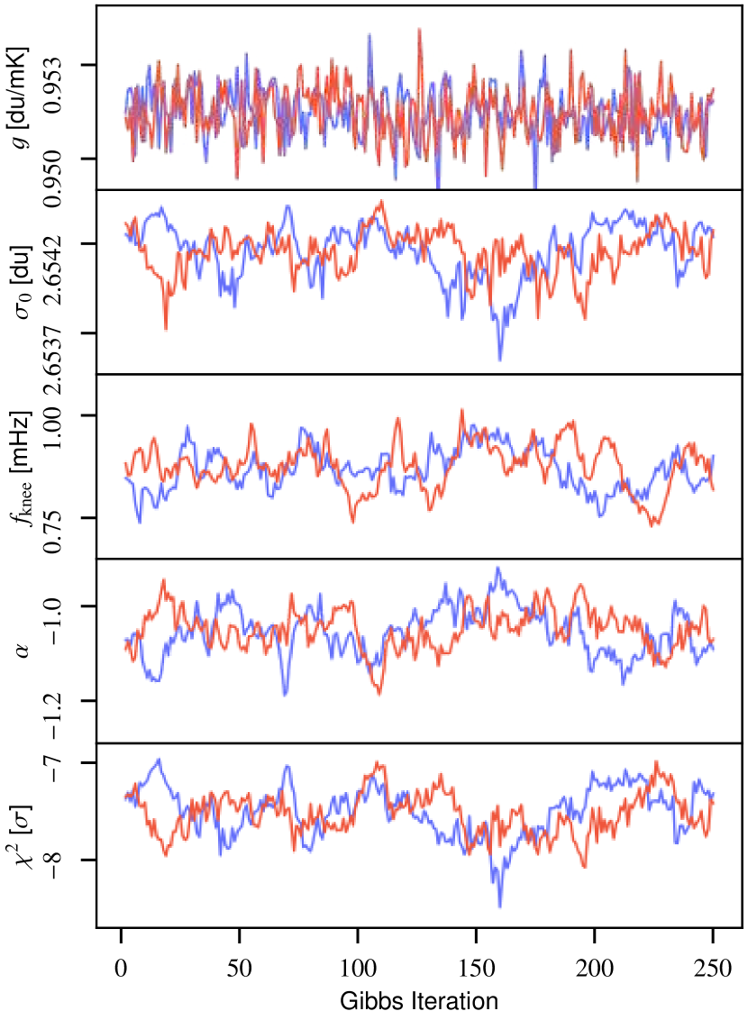
Figure 4: Trace plots of the K113 gain and noise parameters for a single scan starting on MJD 52285.2. The two colors correspond to the two independent Markov chains produced in this analysis.

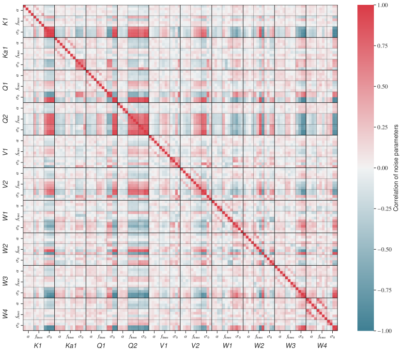
Figure 5: Noise parameter correlation matrix. We average over all Gibbs samples of the noise parameters $\boldsymbol{\xi}_{n}=\{\alpha,f_{\mathrm{knee}},\sigma_{0}\}$ for each PID. We then find the correlation in time between these averages for the different bands and detector. The results here are for the calibrated white noise level, $\sigma_{0}[\mathrm{mK}]$. The values for each detector are ordered 13, 14, 23, and 24.

For the current analysis, which aims primarily to derive posterior-based WMAP frequency maps, we produce a total of 500 main Gibbs samples, divided into two chains. Noting that the computational cost of the W-channel carries almost half of the total expense of the WMAP TOD processing, while being of less scientific importance than, say, the K-band, we choose to only reprocess this channel every fourth main sample. Likewise, we only reprocess the V-band every other main sample, and the LFI 70 GHz sample every fourth sample. The total cost for producing 500 WMAP K, Ka, Q, Planck 30, and 44 GHz samples, 250 V-band samples, and 125 W-band and 70 GHz samples is 210k CPU-hrs, and the total wall time is 33 days. Noting that the BeyondPlanck analysis required 4000 samples to reach full convergence in terms of the optical depth of reionization (Paradiso et al. 2023), a corresponding complete LFI+WMAP analysis will cost about 1.7M CPU-hrs, and take about 9 months of continuous runtime on two cluster nodes. While entirely feasible, this is sufficiently expensive that we choose to perform the analysis in two stages; first we present preliminary frequency maps in the current paper, and use these to identify potential outstanding issues, either in terms of data model or Markov chain stability. An important goal of this phase is also to invite the larger community to study these preliminary maps, and thereby identify additional problems that we may have missed. Then, when all issues appear to have been resolved, we will restart the process, and generate sufficient samples to achieve full convergence.

4 Instrumental parameters

In this section and Sect. 5 we present the main results from the Cosmoglobe DR1 analysis, which may be summarized in terms of the joint posterior distribution. For organizational purposes, we will discuss instrumental parameters, frequency maps, and astrophysical results separately in this and the following two sections. It is important to remember that these results are all derived from one single highly multivariate posterior distribution, and every parameter is in principle correlated with all others. In this section, we focus on instrumental parameters, starting with visual inspection of the basic Markov chains and posterior means, before considering each instrumental parameter in turn.

4.1 Markov chains, correlations and posterior mean statistics

To build intuition regarding the general Markov chain properties, we show in Fig. 4 the Markov chains for the gain and noise parameters for one arbitrary diode (K113) and scan. Each panel corresponds to one single parameter, and the observed variation quantify the uncertainty in that single parameter due to the combination of white noise and correlations with other parameters. Here we see that the different parameters have quite different correlation lengths; the gain (in the top panel) has a very short autocorrelation length, as in just a few samples, while the noise parameters have typical correlation lengths of a few tens of samples. Even for these parameters, however, the full set of 500 samples provides a fairly robust estimate of the full marginal mean and uncertainty.

The bottom panel shows the reduced normalized $\chi^{2}$ for the same scan in units of $\sigma\equiv\sqrt{2n_{\mathrm{TOD}}}$, and we see that this also shows similar correlation lengths as the noise parameters. This makes sense since the TOD residual at the level of a single sample is strongly noise dominated. In contrast, small variations in either the sky signal or gain have relatively small impacts on this particular $\chi^{2}$; the goodness of fit of such global parameters is better measured through map-level residuals and $\chi^{2}$’s. In this respect, we also note that the absolute value of the TOD-level $\chi^{2}$ is for this particular scan about $-7.5\thinspace\sigma$, which at first sight appears as a major goodness of fit failure. However, it is important to recall that a typical scan contains about five million data points, and this statistic is therefore extremely sensitive to any deviation in the noise model. Specifically, the reduced $\chi^{2}$ for this particular scan is $\chi_{\mathrm{raw}}^{2}/n_{\mathrm{TOD}}=0.993$, which corresponds to an overestimation of the white noise level of only 0.3 %. Furthermore, as discussed in Sect. 2.6.1, we currently assume a strict $1/f$ noise model for the WMAP noise, while the true WMAP noise is known to exhibit a very slight non-white noise excess at high frequencies (Watts et al. 2023b). Properly modeling such non-white high-frequency noise is therefore an important goal for the next Cosmoglobe data release. Such work is also a vital step in preparing for integration of other types of experiments with non-white noise into the framework, such as Planck HFI. However, in absolute terms, the impact of this model failure is very limited, and not likely to significantly affect any astrophysical results; it is primarily a limitation for TOD-level goodness of fit testing.

For a survey of the entire experiment’s noise properties, Fig. 5 shows pairwise correlations between the various noise parameters for all DAs, averaged over all Gibbs samples and scans. It is important to note that a non-zero correlation in this plot does not indicate that the specific noise realization is correlated between DAs, but only that the noise PSD parameters are correlated. This is expected due to the WMAP satellite motion around the Sun, which induces an annual variation in the system temperature. This correlation plot therefore primarily quantifies the sensitivity to this common-mode signal for each diode. Most notably, we see that the Q2 DA exhibits particularly strong correlations, and we also note that the calibrated white noise $\sigma_{0}[\mathrm{mK}]=\sigma_{0}[\mathrm{du}]/g$ is generally more susceptible to these variations than $f_{\mathrm{knee}}$ and $\alpha$.

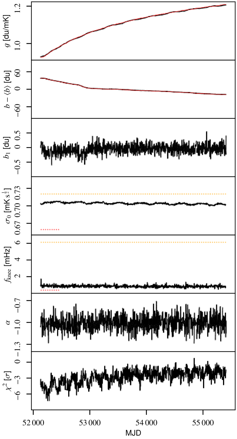
Figure 6: Overview of K113. The red solid lines in the first and second panel are the regressed gain and baseline from WMAP9, while the black lines in all panels are posterior means from the Cosmoglobe Gibbs chain. The red dashed and yellow dashed lines are reported $\sigma_{0}$ and $f_{\mathrm{knee}}$ values from the first-year WMAP data analysis and GSFC measurements, respectively.

Next, in Fig. 6 we show posterior mean values for each instrumental parameter for the same K113 diode, in this case plotted as a function of time throughout the entire mission. The panels show, from top to bottom, 1) gain; 2) the difference between the baseline mean and its full-mission average; 3) the baseline slope; 4) the white noise level; 5) the correlated noise knee frequency; 6) the correlated noise slope; and 7) the TOD-level $\chi^{2}$. The Cosmoglobe results are shown as black curves, while the WMAP results are (for the gain and baseline) shown as red curves; dotted red and orange line corresponds to the first-year WMAP and Goddard Space Flight Center (GSFC) laboratory measurements, respectively. Note that the gain and baseline are nearly indistinguishable – their differences will be discussed in more detail in Sect. 4.2. For brevity, we have only shown the results for one single diode here. However, a complete survey of all instrumental parameter posterior means for all 40 diodes is provided in Appendix A, and all individual samples are also available in a digital format as part of the Cosmoglobe DR1.

4.2 Gain and baselines

We now consider the gain and baseline parameters in greater detail, and aim to compare our estimates with the WMAP9 products. The WMAP9 gain and baseline estimates are not directly available in terms of public data products, but only in terms of the general parametric models. For instance, the WMAP gain model reads (Greason et al. 2012)

$$g=\alpha\frac{\overline{V}-V_{\circ}-\beta(T_{\mathrm{RXB}}-290\thinspace\mathrm{K})}{T_{\mathrm{FPA}}-T_{\circ}}+(m\Delta t+c),$$ (49)

where $\overline{V}$ represents the radio frequency bias powers per detector; $T_{\mathrm{RXB}}$ and $T_{\mathrm{FPA}}$ are the receiver box and focal plane assembly temperatures, which are recorded every 23.04 s; $\alpha$, $\textit{V}_{\circ}$, $\beta$, $T_{\circ}$, $m$, and $c$ are all free parameters that are fit to a constant value across the mission for each diode. Evaluating this model as a function of $T_{\mathrm{RXB}}$ and $T_{\mathrm{FPA}}$ requires the housekeeping data for the thermistor that was physically closest to the relevant radiometer’s focal plane on the satellite. The free parameters are fully tabulated in the WMAP Explanatory Supplement (Greason et al. 2012), but the physical layout of the thermistors in the focal plane and receiver box is not readily available. We therefore do not attempt to reproduce the gain model given in Eq. (49).

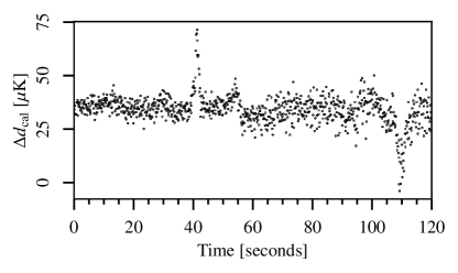
Figure 7: Difference between the Cosmoglobe $\boldsymbol{d}_{\mathrm{cal}}=\boldsymbol{d}/g-\boldsymbol{b}-\boldsymbol{s}_{\mathrm{sl}}$ and the delivered calibrated TOD from WMAP. Note that this is for a small segment of the K113 TOD displayed in Fig. 1.

Rather, we estimate the gains and baselines by comparing the uncalibrated WMAP data with the calibrated WMAP data, after subtracting a far sidelobe contribution convolved with the delivered WMAP9 DA maps plus the Solar dipole. We find that the calibrated and uncalibrated data can be related by

$$d^{\mathrm{raw}}_{t}=g(d^{\mathrm{cal}}_{t}+s^{\mathrm{sl}}_{t})+\sum_{i=0}^{3}c_{i}(t-t_{0})^{i},$$ (50)

where the second term is a cubic polynomial with coefficients $c_{i}$ referenced to the time at the beginning of the scan $t_{0}$. The red curves in the top two panels of Fig. 6 correspond to these estimates. The agreement between the WMAP9 and Cosmoglobe gain and baseline models appear reasonable at this level and for this diode.

A complete comparison between the WMAP and Cosmoglobe gain and baseline models for all diodes is provided in Appendix A. In particular, Fig. A shows the baseline differences as a function of time, and here we see that most diode differences scatter around a constant value that is close to zero; the precise constant value is of limited importance, since that only corresponds to a difference in the overall monopole of the maps, which for WMAP is determined through post-processing. However, there are a few notable features. First, we see that the two Q11 diodes exhibit large variations at the very beginning of the mission, with typical values of a few du’s. Individual scans show notable spikes for many diodes. These are all relatively isolated in time, and will therefore have relatively minor impact on the final maps. Far more significant are the W-band differences, for which one sees both slow drifts and abrupt changes. Furthermore, in many cases they vary notably between diodes within the same DA, which translates into differences in the large-scale polarization maps derived from the two pipelines.

Similarly, Fig. 49 compares the gain solutions directly, while Fig. 50 shows the fractional differences in units of percent. Overall, we see that the two gain models agree to typically about 0.5 % in an absolute sense, and better than typically 0.1 % in terms of relative agreement between neighboring scans. The most striking feature in this plot is an annual variation that traces the WMAP satellite’s motion around the Sun. In general, such an oscillatory gain behaviour is entirely expected, because of known temperature variations in the satellite. However, the difficulty lies in estimating the magnitude of the oscillations, as different radiometers can respond differently to these temperature variations. In this respect, it is useful to recall that the WMAP and Cosmoglobe gain estimation algorithms differ at a fundamental level. The WMAP analysis considers each DA in isolation, fitting seven instrumental parameters, defined by Eq. (49), to the orbital dipole seen by each DA. The Cosmoglobe analysis considers the problem globally, and attempts to fit all gain parameters to the full sky signal (including both the Solar and orbital CMB dipole) simultaneously, without the use of a strong instrumental model prior. Returning to the absolute gains shown in Fig. 49, it is difficult to determine visually which approach is better at this level alone, as the two models are quite similar; in some cases, such as Ka124 and Q214, the WMAP model oscillates more strongly than the Cosmoglobe model, while in others, such as K113 and K114, the opposite is true. We also see the impact of the strong instrumental priors in the WMAP solution particularly well in W-band, where the Cosmoglobe gains are far more noisy than the WMAP gains.

The impact of these differences at the TOD level is illustrated in Fig. 7, which shows the calibrated Cosmoglobe timestream $\boldsymbol{d}/g-\boldsymbol{s}_{\mathrm{sl}}-\boldsymbol{b}$ minus the WMAP calibrated signal in units of microkelvin. The most prominent feature is a $\sim 25\thinspace\mathrm{\mu K}$ offset, which is unsurprising, given the different treatment of baselines in our two pipelines. The second obvious difference is a series of spikes associated with Galactic plane crossings. Differences of order $50\thinspace\mathrm{\mu K}$ are seen where the absolute sky brightness is about $10\thinspace\mathrm{mK}$, equivalent to $\sim 0.5\thinspace\%$ deviations in the gain solution. This is twice as large as the 0.2 % uncertainty estimated in Bennett et al. (2013) based on end-to-end simulations.

Another interesting feature in Fig. 7 is slow correlated variations at a timescale of $\sim$ 20 sec timescale. There is nothing in the Cosmoglobe instrument model that varies on such short timescales, and this must therefore come from WMAP. The most likely explanation is the fact that the WMAP gain model depends directly on housekeeping data that are recorded with a 23.04 sec sample rate, and these values appear to have been applied without any smoothing, resulting in sharp jumps in the final WMAP gain model, as well as increases in the observed level of scatter. At the same time, it is also important to note that the Cosmoglobe gain model does not include any time-varying structure within a single scan, and if any artifacts resulting from this are identified in the current products, it may be worth incorporating housekeeping data in a future Cosmoglobe data release.

4.3 Transmission imbalance

Table 3: Transmission imbalance parameters for each WMAP radiometer as estimated in the current analysis (second column) and in the official 9-year WMAP analysis (third column). Our uncertainties indicate $1\thinspace\sigma$ marginal posterior standard deviations.

Radiometer      $$x_{\mathrm{im}}^{\mathrm{CG}}$$      

K11 .            

K12 .            

Ka11 .            

Ka12 .            

Q11 .            

Q12 .            

Q21 .            

Q22 .            

V11 .            

V12 .            

V21 .            

V22 .            

W11 .            

W12 .            

W21 .            

W22 .            

W31 .            

W32 .            

W41 .            

W42 .            

Closely related to the gain model is the transmission imbalance factor, $x_{\mathrm{im}}$, quantifying the difference between responsivity in the two horns, as described in Sect. 2.1. These are listed for each radiometer in Table 3 for both Cosmoglobe and WMAP9; for Cosmoglobe the reported values correspond to marginal posterior means and standard deviations. The same information is plotted in Fig. 8. Overall, there is a reasonable agreement between the Cosmoglobe and WMAP9 estimates, with the same overall magnitude for each individual radimoeter. At the same time, we do observe several notable differences. There are nearly $4\thinspace\sigma$ differences between the derived K11 radiometer, while for Q-band and W2, the $x_{\mathrm{im}}$ factors are consistently larger by about $1\thinspace\sigma$ for all radiometers. The comparison between W-band and V-band is especially noteworthy, as these are the bands with the most prominent transmission imbalance modes in the WMAP9 maps, especially W4. The uncertainties in Cosmoglobe are also larger for the lower frequency channels than in WMAP9, which can be explained by the dependence of $x_{\mathrm{im}}$ on the varying sky model within Commander3. At the same time, the ratio of uncertainties in W-band varies across radiometers, somewhat depending on the knee frequency of the radiometer in question. Overall, the variation in the noise levels and values is expected because of the larger number of degrees of freedom in the Cosmoglobe model, while the amplitude of the relative agreement shows the robustness of the data to the specific pipeline choices.

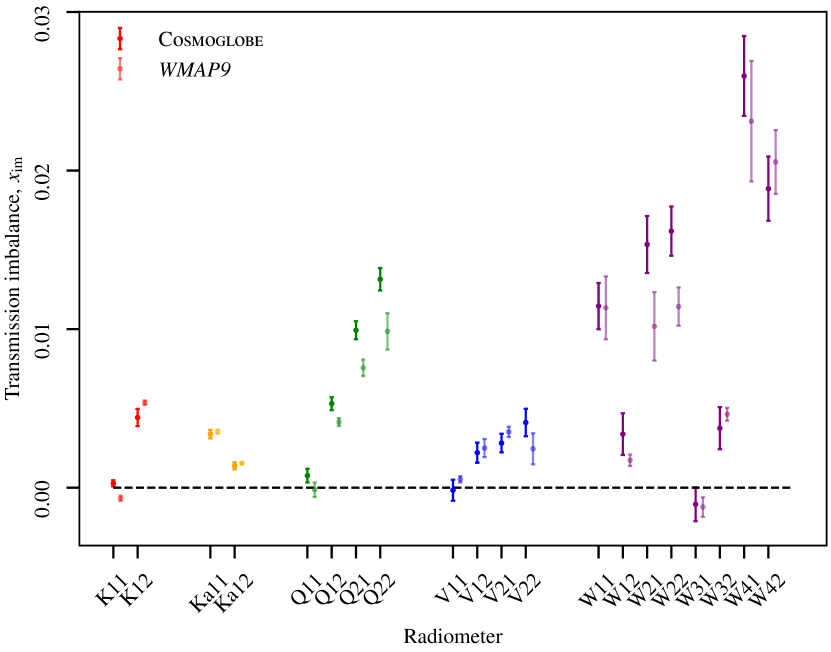
Figure 8: Comparison of the transmission imbalance factors, $x_{\mathrm{im}}$, estimated by Cosmoglobe (dark colors) and WMAP9 (light colors) for each radiometer.

While these differences may appear to be subtle, they could still be important both in terms of final sky map biases and error propagation. The reason for this is that $x_{\mathrm{im}}$ couples directly to the astrophysical sky signal, and in particular to the bright 3 mK Solar CMB dipole. Even an inaccuracy at the $\mathcal{O}(10^{-3})$ level can therefore excite correlated large scale artifacts at the microkelvin level, which are comparable to (or larger than) the expected cosmological reionization of about 0.5 $\mu$K.

It is also important to note that even though the error bars reported in Table 3 are of similar order of magnitude, the detailed manners in which these uncertainties are propagated into higher-level astrophysical results are very different in the two pipelines. Specifically, while the Cosmoglobe sampling approach accounts for all couplings between the specific value of $x_{\mathrm{im}}$ and all other parameters (gain, baselines, correlated noise, CMB dipole, large scale polarization, etc.) at every single step of the Markov chain, the WMAP approach only marginalizes over two linear templates in the low-resolution covariance matrix. These two templates are derived by changing $x_{\mathrm{im}}$ for one diode pair in a DA by +10 % and the other diode pair by $\pm 10$ % with respect to their mean values. This linear low resolution approach can obviously only capture a limited subvolume of the full nonlinear effect of transmission imbalance uncertainties. Even cases for which the mean estimates formally agree within $1\thinspace\sigma$ may therefore in practice result in significantly different sky maps and error estimates. We will return to the impact of transmission imbalance in Sect. 5.3.

Table 4: Summary of noise properties.

Sensitivity, $$\sigma_{0}$$ (mK )      Knee frequency, (mHz)

Radiometer .      Diode GSFC WMAP      GSFC WMAP      

K11 .      1            

     2      

K12 .      1            

     2      

Ka11 .      1            

     2      

Ka12 .      1            

     2      

Q11 .      1            

     2      

Q12 .      1            

     2      

Q21 .      1            

     2      

Q22 .      1            

     2      

V11 .      1            

     2      

V12 .      1            

     2      

V21 .      1            

     2      

V22 .      1            

     2      

W11 .      1            

     2      

W12 .      1            

     2      

W21 .      1            

     2      

W22 .      1            

     2      

W31 .      1            

     2      

W32 .      1            

     2      

W41 .      1            

     2      

W42 .      1            

     2      

4.4 Instrumental noise

Next, we consider the instrumental noise parameters, $\boldsymbol{\xi}_{n}=\{\sigma_{0},f_{\rm knee},\alpha\}$. In this case, we recall three major differences between the Cosmoglobe and WMAP analysis. First, while we model the noise explicitly with a $1/f$ noise profile in Fourier domain, the WMAP analysis adopts a model independent approach by simply measuring the autocorrelation function directly. A notable advantage of the latter approach is that it naturally accounts for the non-white noise at high frequency without algorithmic modifications, while this has to be added manually in the parametric Cosmoglobe approach. A second difference is the fact that while WMAP uses 1- or 24-hour segments to estimate the noise model, we use 3–5 days, and are therefore able to trace noise correlations to longer timescales. Thirdly, while WMAP assumed the noise filter to be constant within each year of operation, we allow it to vary between scans, that is, on a timescale of days.

With these differences in mind, Figs. 51–53 provides a complete overview of the noise parameters for all 40 WMAP diodes. As in Fig. 6, the solid black lines show Cosmoglobe results, while the dotted red and orange lines show the corresponding 1-year and GSFC measurements, where available. Starting with the white noise level, we see that these are overall relatively constant in time, although with slight traces for annual variations in some channels (e.g., K113); slight instabilities near the beginning and/or end of the mission in other channels (e.g., Ka); and slight drifts in yet others (e.g., Q12 and W32).

When comparing the Cosmoglobe values with the WMAP values, it is worth noting that WMAP only published results for each diode-pair, not for individual diodes. All WMAP values are therefore the same for each diode pair. Still, from the Cosmoglobe results, which are reported individually for each diode, we see that diode pairs generally have quite similar white noise levels and vary at most by a percent.

To facilitate a more quantitative comparison, Table 4 compares the Cosmoglobe posterior mean results with the reported WMAP results. Note that for $\sigma_{0}$, the Cosmoglobe values have been scaled by a factor of $\sqrt{2}$, in order to account for the fact that these apply to individual diodes, as opposed to diode-pairs. Both in Table 4 and Fig. 51, we see that about half of the Cosmoglobe values lie between the two WMAP results, while the other half are higher. In particular the W-band noise levels are much higher in the Cosmoglobe solution, sometimes by as much as 50 %.

In this respect, it is worth recalling from Sect. 2.6.1 that the white noise level in raw du is in Cosmoglobe not strictly sampled from the full posterior distribution, but rather estimated deterministically from the highest frequencies. This makes our estimate more sensitive to possible colored noise at high frequencies (Watts et al. 2023b). At the same time, the calibrated white noise level $\sigma_{0}[\mathrm{K}]=\sigma_{0}[\mathrm{du}]/g$ depends on the gain, and this allows us to test the effects of the calibration on the instrument sensitivity itself. The calibrated white noise level follows a biannual trend indicative of a system temperature variation, which is to be expected given the radiometer equation

$$\sigma_{0}[\mathrm{V}]\propto gT_{\mathrm{sys}}.$$ (51)

Aside from an overall amplitude shift due to the absolute calibration variation, the shape of the white noise level is stable throughout the Gibbs chain.

Another issue worth pointing out is the fact that we are not yet accounting for correlations between the white noise in diode pairs. However, the correlation coefficient between residuals is relatively small, with e.g., values of roughly 5 % for K-band. Diode pairs in V and W have higher correlation of $\sim 25\thinspace\%$, but have similar orders of correlation with diodes from the other pair, indicating that the correlation is driven by unsubtracted sky signal.

In summary, we have not yet been able to identify the cause of the major difference in reported white noise levels in the W-band; while we do detect goodness of fit failures of as much as 5–10 $\sigma$ for many of these diodes at the TOD level (see Sect. 4.1), such significances correspond to sub-percent errors in the white noise level. For comparison, a white noise misestimation of 50 % would translate into an 800 $\sigma$ $\chi^{2}$ failure. This is left to be understood through future work, but we do not expect it to indicate a real failure in either analysis, but it is more likely just a matter of different conventions.

Turning our attention to the low frequency parameters, we see in Table 4 and Fig. 52 that our knee frequencies lie between the WMAP ground and laboratory measurements, almost without exception, which on the one hand indicates generally good agreement between the two analyses. However, our values are in fact closer to the WMAP laboratory measurements than the WMAP flight measurements. This may be due to the longer time-scales used in the Cosmoglobe analysis.

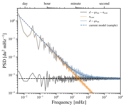
Figure 9: PSD for diode W413 that spans MJDs 52252.3–52254.8. The power spectrum of the blue line corresponds to the residual, while the gray line is the residual with a correlated noise realization removed.

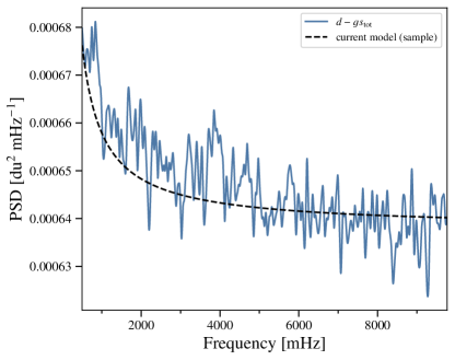
Figure 10: PSD for diode W413 that spans MJDs 52252.3–52254.8. The black dashed line is a sample of the theoretical PSD, while the blue line is the smoothed residual power spectrum.

Most diodes have constant $f_{\mathrm{knee}}$ throughout the mission, with a few notable exceptions. First, all W-band channels display some amount of temporal variation that does not seem to be associated with any sinusoidal features. Second, all Q2 channels, V223, and V224 all display a similar asymptotic drift in time. We have not found any instrumental effects that share this feature. The PSD slope $\alpha$ is around $-1$ for each diode, albeit with high scatter for the lower frequencies. As expected, the uncertainty in $\alpha$ decreases as $f_{\mathrm{knee}}$ increases, since there are more datapoints to fit below $f_{\mathrm{knee}}$ where the constraining power on $\alpha$ is the strongest.

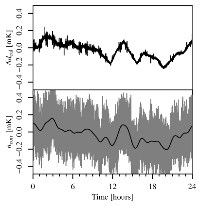
Figure 11: (top): Difference between the Cosmoglobe $\boldsymbol{d}_{\mathrm{cal}}=\boldsymbol{d}/g-\boldsymbol{b}-\boldsymbol{s}_{\mathrm{sl}}$ and the delivered calibrated TOD from WMAP. (Bottom): Raw correlated noise (gray) and smoothed data with Gaussian kernel (black). This shows the hourly baseline subtraction from the WMAP treatment.

For completeness, Fig. 54 shows a summary of the reduced normalized $\chi^{2}$ for all diodes. The most striking features in these figures are the amplitude and semiannual periodicity. Given the noise model and data residual, we can evaluate the goodness of fit in the form of the relative $\chi^{2}$. Here, we find that approximately half of the diodes have a $\chi^{2}$ value at least $6\leavevmode\nobreak\ \sigma$ above or below the expected value. Given perfect Gaussian residuals, we would expect these values to be within $\pm 1\leavevmode\nobreak\ \sigma$ 68 % of the time. For a typical W-band scan of length $n_{\mathrm{TOD}}=2^{22}$, a $10\leavevmode\nobreak\ \sigma$ model failure corresponds to $\chi^{2}/n_{\mathrm{TOD}}=1.003$. It is therefore exceedingly difficult to look at any given WMAP scan in the time domain and identify a model failure. To illustrate this, Fig. 9 compares the observed noise PSD with the best-fit model for the W413 diode. This is a $7\leavevmode\nobreak\ \sigma$ outlier; despite this, the $1/f$ model appears to perform exceedingly well over seven decades in frequency.

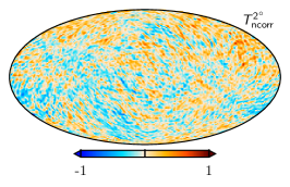
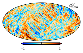
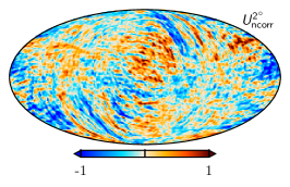
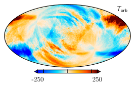
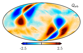
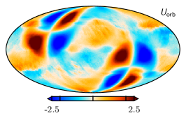
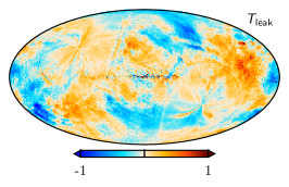
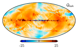
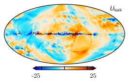
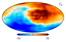
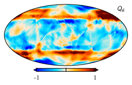
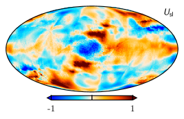
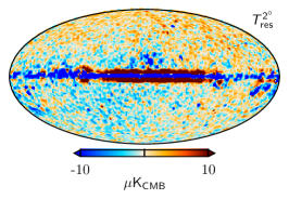
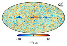
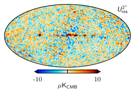
Figure 12: TOD corrections for K-band for a single Gibbs sample, projected into maps. Columns show Stokes $T$, $Q$, and $U$ parameters. Rows show, from top to bottom, 1) correlated noise; 2) the orbital dipole; 3); bandpass mismatch leakage; and 4) sidelobe corrections. The bottom row shows the residual obtained when binning the sky and systematics-subtracted TOD into a sky map. Note that the correlated noise and residual have been smoothed by a $2^{\circ}$ Gaussian beam.

Only with aggressive smoothing does the model failure become apparent at frequencies 1–10 Hz. This is illustrated in Fig. 10, which shows exactly the same underlying data as in Fig. 9, but heavily smoothed. Here, it is clear that despite fitting the data well at the highest and lowest frequencies, it is in the intermediate range of 1–5 Hz where the $1/f$ model is a less accurate fit to the residual power spectrum. Part of the cause of this failure is that the white noise level is fixed by the value of the power spectrum at the Nyquist frequency, as it was computed by differencing adjacent samples. The power spectrum has a downward trend above 1 Hz, indicating that the data would be better fit by a polynomial in powers of $f^{\alpha}$. This is phenomenologically similar to the WMAP collaboration’s approach of describing the time-space autocorrelation as a cubic polynomial in $\log\Delta t$ (Jarosik et al. 2007).

In practice, the failure of the $1/f$ model has a small effect on the final data products, and was not visible in noise models when we modeled the data in one day scans rather than the longer 3–7 day scans due to the lower $n_{\mathrm{TOD}}$ giving a higher uncertainty on the relative $\chi^{2}$. Therefore, although this strictly constitutes a deficiency in the model, it is in practice too small to affect the results of the rest of the chain. The downturn of the noise PSD at high frequencies is also present in, e.g., the Planck HFI data (Planck Collaboration Int. XLVI 2016, Fig. 1), so improved modeling of this form will be a necessity in future Cosmoglobe endeavors, and will be used to improve the WMAP data processing.

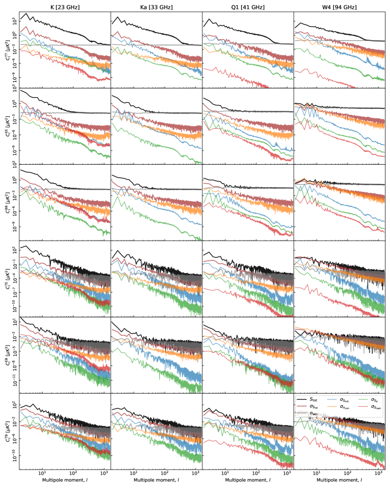
Figure 13: Pseudo-spectrum standard deviation for each instrumental systematic correction shown in Fig. 12 (thin colored lines). For comparison, thick black lines show spectra for the mean of the full frequency map; thick red lines show their standard deviations (i.e., the full systematic uncertainty); and gray lines show white noise realizations. Columns show results for K, Ka, Q1, and W4, respectively, while rows show results for each of the six polarization states ($TT$, $EE$, $BB$, $TE$, $TB$, and $EB$). All spectra have been derived outside the CMB confidence mask presented by Andersen et al. (2023) using the HEALPix anafast utility, correcting only for sky fraction and not for mask mode coupling.

Before concluding this section, we recall the close relationship between the correlated noise component and the baseline model. This is illustrated in Fig. 11, which shows the difference between the calibrated Cosmoglobe and WMAP TOD data for K113, i.e., the same as Fig. 7, but plotted for 24 hours instead of 10 minutes. The bottom panel shows the Cosmoglobe correlated noise realization for the same period, both raw and smoothed. The most prominent feature in this figure is a varying signal of amplitude $0.2\thinspace\mathrm{mK}$. This is due to the hourly baseline subtraction mentioned above, which contrasts with the Cosmoglobe approach of assigning a linear baseline solution for the entire scan, and then accounting for the nonlinearity through $\@vec{n}^{\mathrm{corr}}$. The variations are commensurate with the correlated noise correlation length, which for K113 has ${f_{\mathrm{knee}}\sim 0.5\thinspace\mathrm{mHz}}$, corresponding to a little over half an hour. Therefore, the hour-long baseline subtraction acts as a destriper, removing an estimate of the correlated noise.

4.5 Instrumental corrections in map domain

Returning to the global parametric data model in Eq. (6), it is useful for intuition purposes to project each of the WMAP TOD-level correction terms into sky maps. This is done for K-band in Fig. 12, in the same form as was done for LFI by Basyrov et al. (2023). Columns correspond to Stokes $T$, $Q$, and $U$ parameters, while rows show, from top to bottom, 1) correlated noise; 2) the orbital CMB dipole; 3) bandpass leakage; and 4) sidelobe corrections. The bottom row shows the residual obtained after subtracting all modeled terms from the raw TOD. All maps correspond to one single and randomly selected Gibbs sample.

Starting with the correlated noise in the top row and the residual in the bottom row, we note that these are the only terms that are fundamentally stochastic in nature; all the instrumental terms are either primarily deterministic in nature, as they rely only on the sky model coupled to a small number of instrumental parameters, such as the gain, bandpass, or beam, whereas the random realizations of the sky model are highly constrained by the multifrequency component separation. As such, the correlated noise and residual maps act as the “trash cans” of Bayesian CMB analysis; together they show anything in the TOD that is not explicitly modeled. For the K-band channel, we see that the correlated noise is limited to less than 1  $\mu$K over almost the full sky, while the residual appears like random noise over most of the sky. The main exceptions to this are strong residuals near the Galactic plane in temperature, which indicates the presence of unmodeled foreground features; typical candidates to explain this would be curvature in the synchrotron spectral index or a more complicated AME SED than that assumed here. Secondly, at high latitudes we see traces of a small dipole with an amplitude of 1–2 $\mu$K aligned with the CMB dipole. This indicates the presence of an absolute calibration deviation of about 0.03–0.06 %; this is within the uncertainty of the absolute K-band calibration prior of 0.1 % discussed in Sect. 2.4, and when inspecting different Markov chain samples of the same type, one can see that the amplitude and sign of this residual scatter is around zero as expected.

Next, the amplitude of the orbital dipole is about 250 $\mu$K in temperature and 2.5 $\mu$K in polarization. This component by itself is exceedingly well known, as it depends only on the satellite velocity and the CMB monopole temperature. However, when actually fitting this to the real data, it obviously also depends on both the gain, and sample-to-sample variations in this map, and is therefore a good tracer of gain uncertainties. In addition, its physical appearance also in principle depends on the sidelobe model, but we do not yet propagate sidelobe uncertainties anywhere in the analysis.

The third row shows the corrections for bandpass leakage. As for Planck LFI, this term is by far the largest correction in polarization, with an amplitude that is almost an order of magnitude larger than any of the others. It is highly nontrivial to compare this component to the WMAP9 analysis, since this effect was accounted for by solving for a spurious $S$ map as part of their mapmaking. However, it is important to note that whether one models this effect explicitly, as we do, or project it out during mapmaking, as the WMAP pipeline did, the accuracy of the bandpass corrections depends directly on the accuracy of the gain and transmission imbalance calibration.

The fourth row shows the sidelobe contribution. Here we see that the temperature amplitude reaches 50  $\mu$K, which corresponds to 1.5 % of the CMB Solar dipole amplitude. If it should turn out that the sidelobe model were incorrect by, say, 30 %, this translates directly into an error in the absolute K-band calibration of about 0.5 %, which is significantly greater than the statistical error shown above. Given the degeneracies discussed in Sect. 2.4, there is thus also a strong degeneracy between the AME dipole and the K-band sidelobe. For polarization, the amplitude is mostly smaller than 1 $\mu$K, and therefore of minor importance for this channel. We note that only the intensity component of the WMAP sidelobe model has been published, and polarized sidelobes are not accounted for in the current processing. However, as shown by Barnes et al. (2003)’s Table 2, the amplitude of this contribution is relatively small, with a high-latitude mean of $0.8\thinspace\mathrm{\mu K}$ for K-band and $<0.1\thinspace\mathrm{\mu K}$ for all other bands.

4.6 Instrumental uncertainties in power spectrum domain

We conclude this section by estimating the uncertainty of each instrumental effect in terms of angular power spectra, using the same methodology as Basyrov et al. (2023) for Planck LFI. That is, we first compute the power spectra for each individual instrumental correction Markov chain sample, as illustrated in Fig. 12, and then compute the standard deviation of all these samples. The results from this computation are summarized in Fig. 13 for four DAs, namely K, Ka, Q1, and W4. In each panel the black line shows the power spectrum of the full coadded frequency sky map (including both signal and noise), while the gray line shows the white noise level. The thick dark red line shows the sum of all variations, while the thin colored lines show the contribution from individual correction terms.

On large angular scales in the $TT$ spectrum, we see that the dominant uncertainty comes from the orbital dipole (blue lines), which trace gain uncertainties. This is reasonable, since these data are strongly signal-dominated; indeed, for K-band even the sidelobe contribution (green lines) is higher than the correlated noise.

For large-scale $E$-mode polarization, the dominant term varies from channel to channel. Specifically, for K-band the bandpass leakage (thin red lines) and gain fluctuations are significantly larger than the correlated noise, while for Q1 and W-band the correlated noise dominates for most multipoles, although the gain fluctuations are comparable for some $\ell$’s.

An important conclusion to be drawn from these measurements is that a simple uncertainty model that primarily accounts for correlated noise is likely to be suboptimal for detailed cosmological analysis of large-scale polarization. Both gain and bandpass uncertainties are at least as important for the lowest multipoles, and simultaneously accounting for all of these contributions is important in order to derive robust cosmological results.

5 Frequency maps

In this section, we discuss the reprocessed WMAP frequency maps and their properties. In Sect. 5.1 we present the reprocessed WMAP maps themselves, commenting on notable features in the maps themselves, as well as differences with the WMAP9 results. In Sect. 5.2 we focus on the consistency of our new maps, both internally among the WMAP channels, and with respect to Planck. Section 5.3 describes the efficiency of template-based transmission imbalance uncertainty propagation.

5.1 Map survey

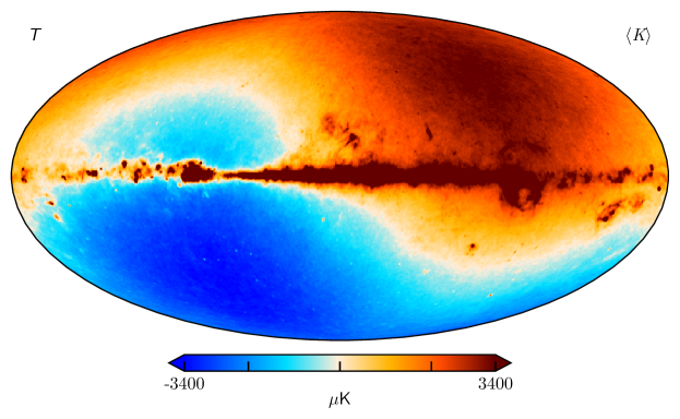
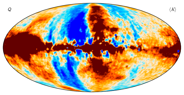
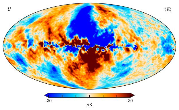
Figure 14: Posterior mean K-band map produced with the Cosmoglobe pipeline. Rows show Stokes $T$, $Q$, and $U$, respectively. The temperature map is shown at full resolution, while the polarization maps are smoothed with a $2^{\circ}$ FWHM Gaussian beam to reduce small-scale noise.

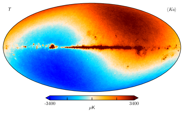
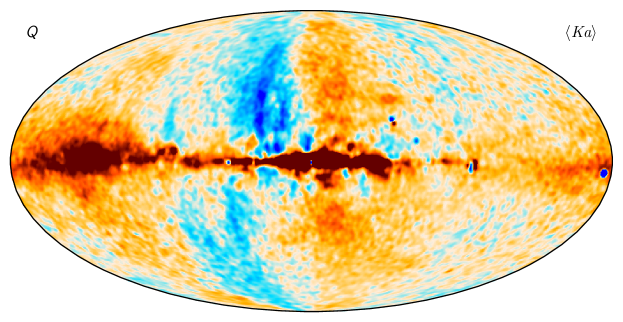
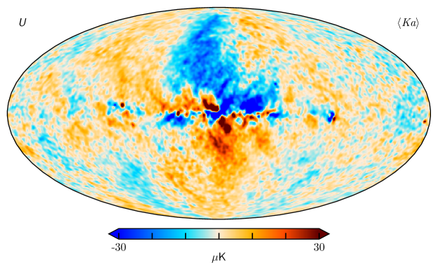
Figure 15: Same as Fig. 14, but for Ka-band.

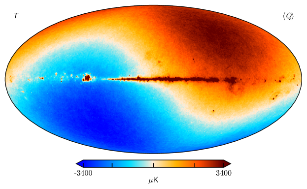
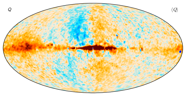
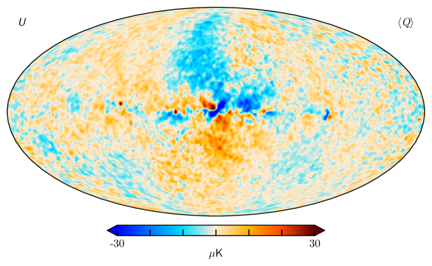
Figure 16: Same as Fig. 14, but for Q-band.

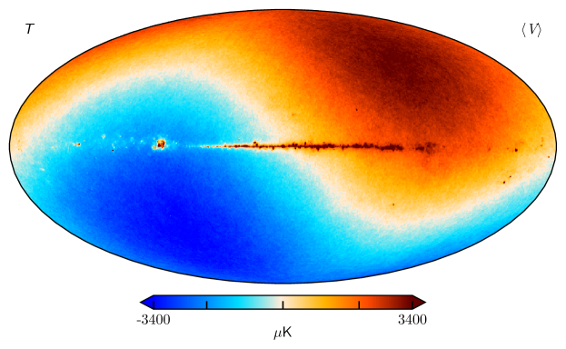
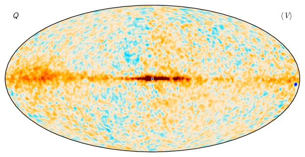
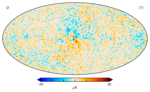
Figure 17: Same as Fig. 14, but for V-band.

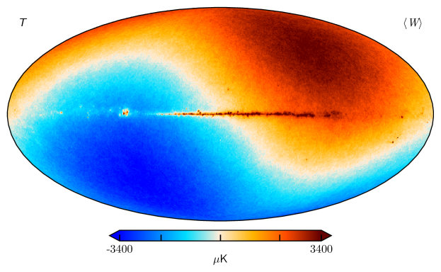
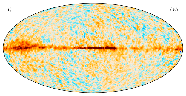
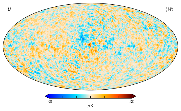
Figure 18: Same as Fig. 14, but for W-band.

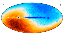
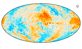
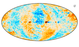
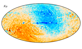
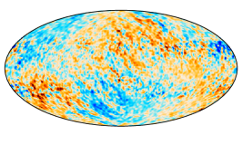
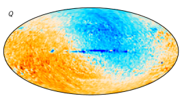
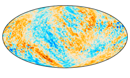
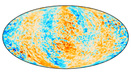
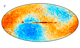
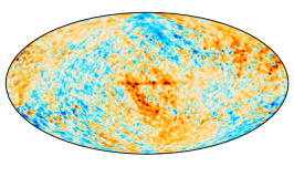
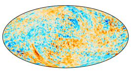
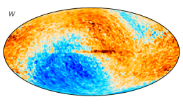
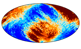
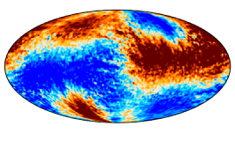
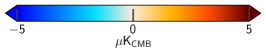
Figure 19: Difference maps between the Cosmoglobe and 9-year WMAP frequency maps. Columns show Stokes $T$, $Q$, and $U$ parameter maps, while rows show K-, Ka-, Q-, V-, and W-band maps. The maps are all smoothed with a $2^{\circ}$ FWHM Gaussian beam.

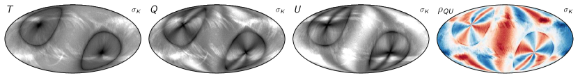
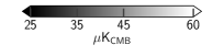
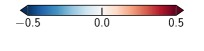
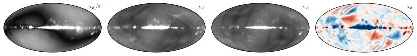
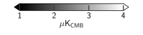
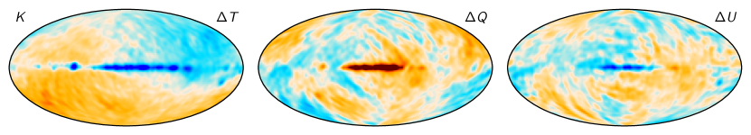
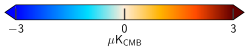
Figure 20: Posterior variation maps for K-band. Columns show the Stokes parameters and the correlation coefficient between $Q$ and $U$, while the rows show (top) the white noise rms per pixel and (bottom) the posterior standard deviation. The rms maps are unsmoothed, while the standard deviations have been smoothed to $7^{\circ}$.

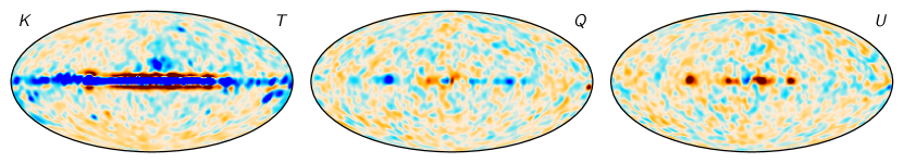
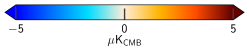
Figure 21: Difference between two K-band Gibbs samples, smoothed to $7^{\circ}$.

Figure 22: TOD-level residual map for K-band, smoothed with a $5^{\circ}$ FWHM Gaussian beam.

We start by showing the co-added frequency K-band, Ka-band, Q-band, V-band, and W-band posterior mean maps in Figs. 14–18, all defined in thermodynamic $\mu\mathrm{K_{CMB}}$ units. All maps are produced at the DA level, and in these figures the Q, V, and W-band maps are generated by inverse-variance weighting the individual DAs. The temperature maps are presented at full angular resolution, while the polarization maps have been smoothed with a $2^{\circ}$ Gaussian beam to reduce small scale structure and make the larger scale effects more apparent. Overall, the temperature maps behave as expected from the official WMAP analysis, with falling foreground amplitudes with frequency. Furthermore, it is very difficult indeed, if not impossible, to see visual differences between the Cosmoglobe and WMAP maps by eye when switching rapidly between them. However, it is important to note that the Cosmoglobe frequency maps retain the Solar CMB dipole, following Planck Collaboration LVII (2020) and BeyondPlanck (2023), while it is removed in the WMAP official maps. Similarly, we see that the amplitudes of the polarized maps decrease as expected from K–V-band following the expected synchrotron behavior, with a slight increase at W-band due to the contribution of thermal dust.

Next, in Fig. 19, we show corresponding difference maps between the official 9-year WMAP maps and the maps produced in this work. The color scale in this plot is linear with range $\pm 5\thinspace\mu$K, and we see that the differences are thus quite small, typically smaller than 1–2 $\mu$K for most channels. The main exception to this is W-band polarization, for which the differences are generally larger than $5\thinspace\mu$K.

Going into greater detail and starting with total intensity, we see first that the K-band difference is dominated by a dipole with a $\sim$ 2.5 $\mu$K amplitude that is anti-aligned with the CMB Solar dipole. In addition, the Galactic plane is slightly brighter in WMAP9 than Cosmoglobe. Both of these suggest that our total absolute K-band calibration is lower than the WMAP9 value by about 0.1 %; given the major differences in methodology described in Sect. 2, this degree of agreement is a major validation of the data and the two pipelines. A similar small dipole difference is also seen in the Q-band.

For the remaining channels, and in particular for the V- and W-bands, the main intensity difference takes the form of a quadrupole with an amplitude of 2–3 $\mu$K aligned with the CMB dipole. Naively, one could suspect this to be due to different treatments of the relativistic quadrupole. However, as noted by Larson et al. (2015), the WMAP9 maps retain the kinematic quadrupole, as does Commander3; in our framework, this signal term is accounted for through the signal model defined in Eq. (10). This is notably different from the Planck maps, which do remove the relativistic quadrupole from the frequency maps (Planck Collaboration II 2020; Planck Collaboration III 2020). Additionally, even though the observed quadrupole has the expected shape, the frequency dependence is not consistent with the expected functional form $x\coth x$ where $x=h\nu/(2kT_{\mathrm{CMB}})$ (Notari & Quartin 2015). For now, we speculate that these differences are rather due to second-order gain or baseline differences, possibly associated with the annual oscillatory structures seen in Fig. 50.

In polarization, we note large scale differences in both Stokes $Q$ and $U$. These differences do not match known Galactic component morphologies, but are more reminiscent of the poorly measured transmission imbalance modes discussed by Jarosik et al. (2011), although the map-space morphologies are not identical. In general, such large mode differences are due to at least three main effects: 1) incomplete polarization angle coverage for a few large-scale modes; 2) errors in transmission imbalance coupled with the Solar dipole; and 3) interplay between the transmission imbalance, the far sidelobe, and the Solar dipole, as briefly described in Sect. 2.1. The scale of these effects is most pronounced in the W-band polarization results, where we see the largest differences between the two processing pipelines.

From these differences alone, it is not possible to determine whether the excess structures are present in the Cosmoglobe or WMAP maps, or both. However, Appendix B provides a complete survey of the Cosmoglobe frequency maps, and in particular Fig. B compares these with the WMAP9 maps. In this case, one clearly sees that the large-scale modes are predominantly present in the WMAP maps, rather than Cosmoglobe.

Returning to the internal properties of the Cosmoglobe posterior distribution, we show in the top panel of Fig. 22 the K-band white noise standard deviation per pixel in Stokes $T$, $Q$ and $U$; the fourth column shows the correlation coefficient between the $Q$ and $U$ coefficients. The bottom panel shows the corresponding posterior standard deviation per pixel. It is important to note that the white noise is not a free parameter in the data model, and there is no white noise component in the Gibbs sampler described by Eqs. (19)–(LABEL:eq:param_samp). That also implies that there is no marginalization over white noise in the resulting frequency map ensemble. Rather, the full marginal uncertainty per frequency map pixel must be obtained by adding the two rows in Fig. 22 in quadrature. However, a preferable approach to performing error propagation for higher level scientific analyses is to analyze each sample separately, taking into account only white noise for each sample, and then use the full sample ensemble as the final result. This is the only robust way of fully accounting for all correlations between the various effects.

The white noise pattern for $T$ follows the usual pattern with highest sensitivity at the North and South ecliptic poles, as well as circles around the poles corresponding to times when the partner horn is observing the opposite ecliptic pole. There are also regions of higher noise level corresponding to planets crossing the ecliptic, and regions of higher emission $\simeq 140^{\circ}$ away from the Galactic center, which correspond to the times when the partner horn lies within the processing mask.

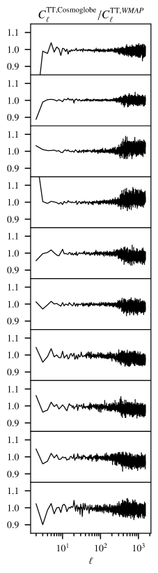
Figure 23: Comparison of the $C_{\ell}^{\mathrm{TT}}$, $C_{\ell}^{\mathrm{EE}}$, and $C_{\ell}^{\mathrm{BB}}$ from WMAP9 and Cosmoglobe. Each row corresponds to a different DA, with frequency increasing from top to bottom. (left): ratio of $C_{\ell}^{\mathrm{TT}}$ from Cosmoglobe compared to WMAP9. (middle/right): $C_{\ell}^{\mathrm{EE/BB}}$ power spectra with WMAP9 in blue and Cosmoglobe in orange.

The polarized RMS maps share all of these characteristics, but with an overall amplitude shift due to polarization measurements having half the effective number of observations per pixel. In addition, the poles have a characteristic “X”-like structure that is rotated $45^{\circ}$ degrees between $Q$ and $U$, corresponding to different polarization orientations. There are also characteristic large scale structures visible in Galactic coordinates, corresponding to polarization modes poorly constrained by the WMAP scan strategy.

While the maps in the top row of Fig. 22 are directly comparable to the corresponding WMAP9 products, the posterior standard deviation shown in the bottom row has no equivalent in the official WMAP release. These maps can be considered the “systematic” error contributions, as their variation depends on the sampled instrumental parameters, i.e., gain, imbalance parameters, correlated noise, and sidelobe correction. The temperature map contains a clear quadrupole signature. This is due to the variation in the absolute calibration $g_{0}$, which changes the Solar dipole in the final map. In addition to the quadrupole, the Galactic plane also varies due to the gain solution’s fluctuations. As expected, the white noise patterns associated with the scan strategy also appear in the polarization maps, which have much lower signal-to-noise ratio than the temperature map.

Another useful quantity is the difference between two arbitrary samples, which we show in Fig. 22. In temperature, the most striking term is a dipole, corresponding to the absolute gain difference, and the Galactic plane. There are also additional weaker lines associated with the scanning strategy, corresponding to different correlated noise and time variable gain realizations. In polarization, gain variations, bandpass uncertainties, and correlated noise dominate the differences between two samples, as quantified in Fig. 13. The polarization differences are aligned with WMAP’s scans, modulated by the polarization angle.

Finally, the quality of the model in map space can be evaluated quite well by looking at the calibrated residual map, i.e., mapping the time-ordered residual $\boldsymbol{r}\equiv(\@vec{d}-\@vec{n}^{\mathrm{corr}})/\boldsymbol{g}-\boldsymbol{s}^{\mathrm{tot}}$. We display this TOD residual for the K-band in the bottom panel of Fig. 12 ($2^{\circ}$ FWHM) and Fig. 22 ($5^{\circ}$ FWHM). In temperature there is a large residual along the Galactic plane, which is to be expected for both temperature and polarization, due to the complexity of the Galactic center. The temperature residual also contains a $\sim 3\thinspace\mathrm{\mu K}$ dipole due to the prior sampling of $g_{0}$ – drawing a sample based on the sky model would track the dipole much more closely, whereas the prior sampling by definition does not use the sky model to draw $g_{0}$. Other than the Solar dipole, Galactic plane, and point sources, both the temperature and polarization maps are visually consistent with white noise across the entire sky.

Again, we have for brevity primarily focused on the K-band in this discussion. For completeness, however, similar plots for all DAs are shown in Appendix B. In particular, Fig. B compares the Cosmoglobe and WMAP DA polarization maps, Figs. 56 and 57 shows the white noise and posterior rms’s, Fig. 58 shows sample differences, and Fig. 60 shows TOD residual maps.

In Fig. 23 we compare angular power spectra computed from both Cosmoglobe and WMAP9 frequency maps. These spectra are derived using the NaMaster (Alonso et al. 2019) compute_full_master routine, while applying the extended WMAP temperature analysis mask which allows a sky fraction of 68.8 %. As the $TT$ power spectrum is strongly signal-dominated for $\ell\lesssim 200$ for all DAs, it is particularly informative to consider ratios, which we show in the left column of Fig. 23. Here we see that the $TT$ spectra derived from the two pipelines are consistent to sub-percent level at all but the very largest and smallest scales for all DAs. We speculate that the large scale differences are due to different CMB Solar dipoles – as noted above, the Cosmoglobe maps retain the Solar CMB dipole, and an estimate of this must be subtracted before evaluating these spectra. In contrast, the WMAP maps have this contribution removed at the TOD level; small differences due to these different treatments are not unexpected. The small scale differences above $\ell\sim 200$ can be attributed to different data selections and low-level processing. For instance, the Cosmoglobe maps exploit about 1 % less data than WMAP9; Cosmoglobe fits one $\sigma_{0}$ parameter per scan, while WMAP9 assumes it to be constant for each year; the WMAP gain model varies every 23 sec, while the Cosmoglobe model assumes constant gain per scan etc.

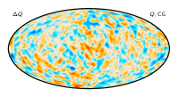
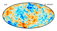
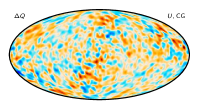
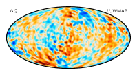
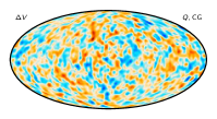
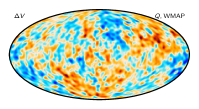
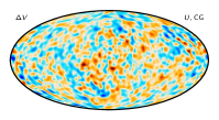
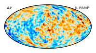
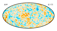
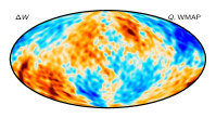
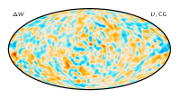
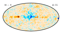
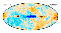
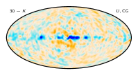
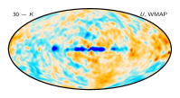
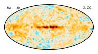
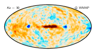
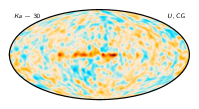
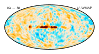
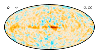
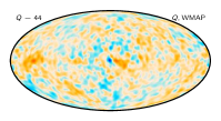
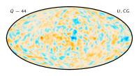
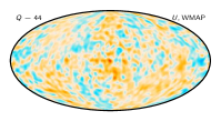
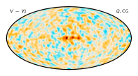
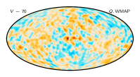
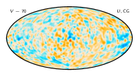
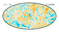
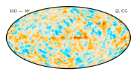
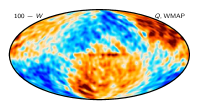
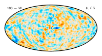
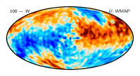
Figure 24: Internal WMAP difference maps, smoothed by $10^{\circ}$. The two left columns are Stokes $Q$, and the two right columns are Stokes $U$, with the Cosmoglobe and WMAP9 maps alternating between columns. The top to bottom rows are difference maps in increasing frequency.

Figure 25: Difference maps between similar WMAP and Planck frequency maps. The comparison plots go, by column: Stokes $Q$ for the Cosmoglobe-produced WMAP and Planck sky maps, Stokes $Q$ for official WMAP and BeyondPlanck data products, Stokes $U$ for the Cosmoglobe sky maps, and Stokes $U$ for the official data products. (Top row): WMAP LFI 30 GHz minus K-band, scaled by the synchrotron power-law. (Top middle row): WMAP Ka-band minus LFI 30 GHz, also scaled by the synchrotron power-law. (Middle row): WMAP Q-band compared to the LFI 44 GHz sky maps, scaled by the synchrotron power-law. (Bottom middle row): WMAP V-band minus LFI 70 GHz, with unit scalings for each band. (Bottom row): The Planck DR4 100 GHz map minus the WMAP W-band  also with unit scalings for each band.

The $E$-mode power spectra, displayed in the second column of Fig. 23, are mainly dominated by noise and polarized synchrotron emission. As expected, the large scale foreground-dominated multipoles decrease in amplitude according to the relative amplitude of the synchrotron spectrum. Overall, the Cosmoglobe and WMAP9 power spectra appear fairly consistent for the K–Q channels, while at V- and W-band there is noticeably more scatter at low multipoles in the WMAP9 spectra than in the Cosmoglobe spectra.

The $B$-mode power spectra, displayed in the third column of Fig. 23, are expected to follow a similar pattern, but since foregrounds are generally reduced by a factor of $\simeq 2$–4 (Bennett et al. 2013; Planck Collaboration IV 2018), this spectrum is less signal-dominated, and therefore more susceptible to instrumental systematics. For instance, the $C_{\ell=3}^{\mathrm{BB}}$ mode has been identified as being particularly poorly constrained due to its symmetry aligning with $\gtrsim 10\thinspace\mathrm{min}$ signals in the TOD induced by the WMAP scan strategy (e.g., Jarosik et al. 2011). In this figure, it appears that these low-$\ell$ modes appear significantly better constrained in the Cosmoglobe maps than in WMAP9 for V- and W-bands, and the overall large scale noise level is lower by one or two orders of magnitude.

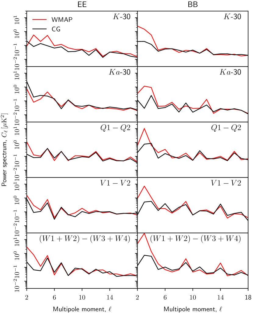
Figure 26: Full sky half-difference spectra. The red lines are the power spectra of the WMAP9 difference maps, while the black lines are the same for the reprocessed Cosmoglobe maps.

5.2 Consistency tests through inter-channel difference maps

As described in Sect. 2.1, the Q- and V-bands each had two DAs, while the W-band had four DAs, and computing differences between the corresponding DA maps can highlight mismodeled systematics. While the K-band and Ka-band have different central frequencies, they are close enough that we can compare them by scaling K-band assuming a polarized synchrotron power law SED of $\beta_{\mathrm{s}}=-3.1$. Similarly, internal differences between scaled K, Ka, and LFI 30 GHz maps provide an important null test. In particular, the K–30 difference has received significant attention ever since the Planck 2015 data release (Planck Collaboration I 2016), showing clear signatures of instrumental systematics. These were gradually reduced through improved Planck processing in the Planck 2018 (Planck Collaboration II 2020), PR4 (Planck Collaboration LVII 2020), and BeyondPlanck (BeyondPlanck 2023) data releases. Still, even after all these developments, large-scale residuals remained that were difficult to resolve through further LFI improvements (Gjerløw et al. 2023). In this section, we revisit this question for the Cosmoglobe products.

We start by inspecting internal WMAP half-difference maps of the form $(Q1-Q2)/2$ etc. These are plotted in Fig. 25. Here we see that the Q-band and V-band half-difference maps from Cosmoglobe have virtually no trace of poorly measured modes, and the differences appear to be well-traced by the rms maps. In contrast, the WMAP half-difference maps show clear evidence of large-scale residuals. The largest visual improvement is in the W-band, where the Cosmoglobe case is almost entirely consistent with instrumental noise, as opposed to the WMAP9 difference that is dominated by large-scale residuals.

Next, Fig. 25 shows comparisons between the WMAP $K$- and $Ka$-bands and the LFI 30 GHz channel, between the WMAP $Q$-band and LFI 44 GHz, and finally between WMAP $V$-band and LFI 70 GHz. When comparing WMAP9 maps with Planck LFI, we use BeyondPlanck products, which represent the cleanest version of Planck LFI published to date. For the Cosmoglobe map comparison, both WMAP and Planck maps were produced by this joint analysis. Additionally, we compare the mean W-band maps with the Planck HFI DR4 100 GHz channel. It is worth noting that this 100 GHz map has had no input from Commander3 so this difference map is an independent comparison between two datasets and processing methods.

Starting with the Cosmoglobe maps, we see in the first and third columns of Fig. 25 that the magnitude of the differences are small in both Stokes $Q$ and $U$. Overall, across all five frequency map comparisons we see small levels of variation, with structure contained to the Galactic plane. Notably, however, there is a larger sky signal within the $\mathit{Ka}-30$ Stokes $Q$ comparison. This large-scale difference also exists in the $\mathit{Q}-44$ Stokes $Q$, but it did not appear in the internal Q half-difference map.

Columns two and four of Fig. 25 show corresponding differences between the official WMAP9 and BeyondPlanck LFI frequency maps. Similar to the Cosmoglobe sky map comparisons, we see differences in the Galactic center, and to a lesser degree along the Galactic plane due to the slight differences in the frequency coverage. When comparing the official WMAP maps, particularly for K-band, we see structures sweeping across large angular scales across the sky, likely due to the poorly measured modes in K-band.

Of particular note is the $100-\mathit{W}$ difference map. The Cosmoglobe difference maps here have a similar level of white noise and Galactic contamination as the $\mathit{V}-70$ maps, whereas the WMAP9 differences are driven by obvious transmission imbalance modes, each with an opposite sign and magnitude. The difference between 100 GHz and W demonstrates that the good agreement between the WMAP and Planck LFI is not simply due to fitting low-level parameters in a joint analysis framework – by obtaining W-band maps that are consistent with an independent 100 GHz polarization map, we have shown that the WMAP-LFI agreement is the result of a genuine improvement in data processing.

Table 5: Transmission imbalance template amplitudes for each WMAP radiometer as estimated by fitting the official templates to low-resolution difference maps between Cosmoglobe and WMAP. The templates are provided in mK, and the template amplitudes are therefore dimensionless. The fourth column lists the fractional decrease in standard deviation, $\Delta\sigma/\sigma\equiv\sqrt{\sigma_{\mathrm{raw}}^{2}-\sigma_{\mathrm{corr}}^{2}}/\sigma_{\mathrm{raw}}$, after subtracting the best-fit templates.

DA      $$a_{1}$$            

K1 .                  

Ka1 .                  

Q1 .                  

Q2 .                  

V1 .                  

V2 .                  

W1 .                  

W2 .                  

W3 .                  

W4 .                  

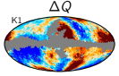
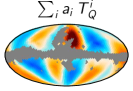
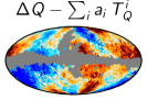
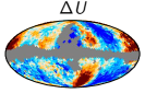
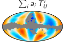
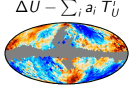
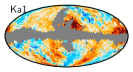
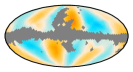
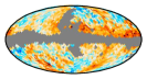
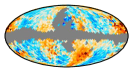
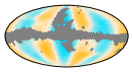
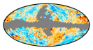
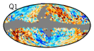
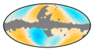
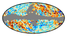
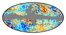
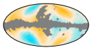
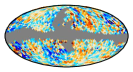
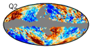
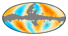
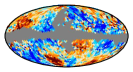
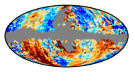
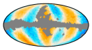
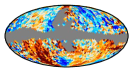
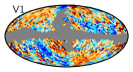
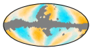
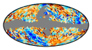
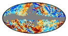
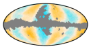
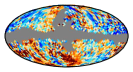
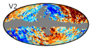
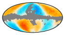
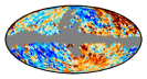
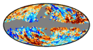
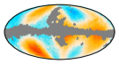
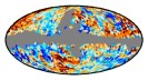
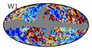
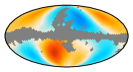
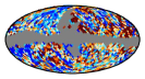
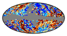
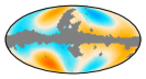
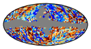
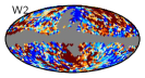
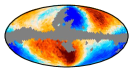
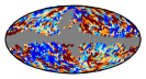
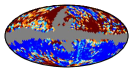
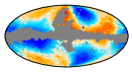
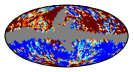
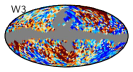
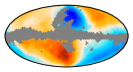
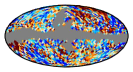
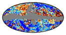
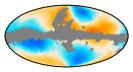
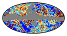
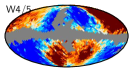
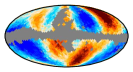
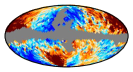
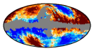
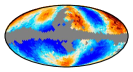
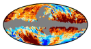
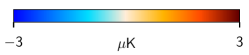
Figure 27: Efficiency assessment of the WMAP approach for transmission imbalance error propagation. The left and right sections of the figure correspond to Stokes $Q$ and $U$ parameters, respectively, while rows show different DAs. Within each section, the left panel shows the raw difference between the WMAP9 and Cosmoglobe DA maps, while the middle panel shows the best-fit WMAP transmission imbalance template combination; the right panel shows the difference between the two. Only one template amplitude is fit for both $Q$ and $U$.

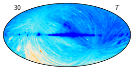
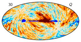
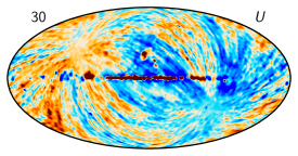
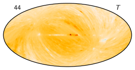
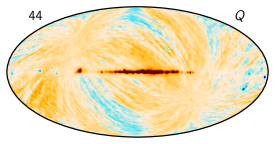
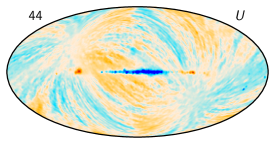
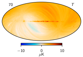
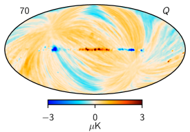
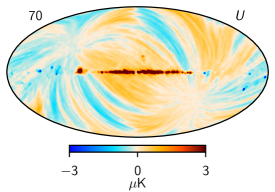
Figure 28: Difference between Cosmoglobe and BeyondPlanck posterior mean frequency maps for 30 (top row), 44 (middle row), and 70 GHz (bottom row). Columns show Stokes $T$, $Q$, and $U$ parameters.

Finally, as noted by Jarosik et al. (2011) the low-$\ell$ W-band polarization data were excluded entirely from the cosmological analysis due to excess variance in the $\ell\leq 7$ multipoles. To test the Cosmoglobe maps’ performance at these scales, we take the power spectrum of the full-sky difference maps using the standard anafast routine in Fig. 26. With very few exceptions, the WMAP9 power spectra have much more power at $\ell\leq 7$ than the Cosmoglobe maps in both the $E$-modes and $B$-modes. Of particular note is the $\ell=3$ $B$-mode, which has consistently been identified as poorly measured in the WMAP scan strategy, and has been reduced in every difference spectrum. Based on these power spectra alone, there does not appear to be a strong justification for excluding the reprocessed W-band polarization data in future cosmological analyses.

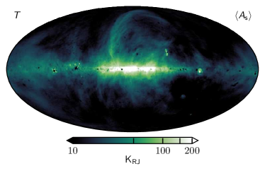
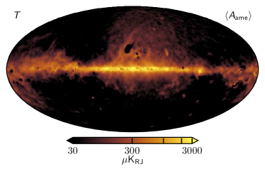
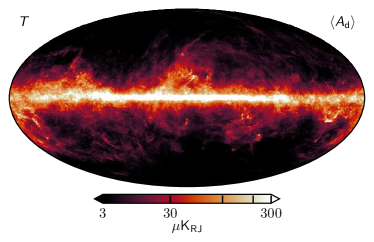
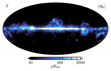
Figure 29: Foreground intensity maps, evaluated at their respective reference frequencies. (Top left:) Synchrotron emission evaluated at 408 MHz. (Top right:) Anomalous microwave emission evaluated at 22 GHz. (Bottom left:) Free-free emission at 40 GHz. (Bottom right:) Thermal dust emission at 70 GHz.

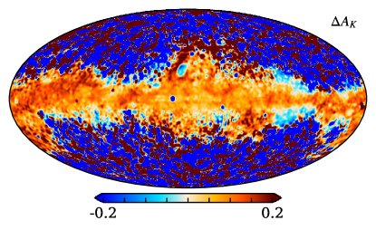
Figure 30: Fractional difference map between the sum of AME and free-free emission at 22 GHz between the Cosmoglobe and BeyondPlanck foreground modes, i.e., $\Delta A_{\mathrm{K}}=s^{\mathrm{CG}}_{\mathrm{AME}+\mathrm{ff}}-s^{\mathrm{BP}}_{\mathrm{AME}+\mathrm{ff}})/s^{\mathrm{BP}}_{\mathrm{AME}+\mathrm{ff}}$.

Based on these calculations, we conclude that the modes that are nearly degenerate by the WMAP scanning strategy, and have represented a major challenge for the official WMAP processing for more than a decade, appear to have been properly regularized by the global Cosmoglobe processing. The frequency maps do not show any evidence of either poorly constrained transmission imbalance modes or other large-scale artifacts, and they are more self-consistent than the WMAP9 frequency maps.

5.3 Efficiency of template-based transmission imbalance uncertainty propagation

Next, we revisit the issue of transmission imbalance error propagation in the official WMAP approach. The WMAP9 likelihood deweights estimates of the transmission imbalance modes in the low resolution polarization likelihood covariance matrix, so that accurate power spectra could be obtained from the maps (Jarosik et al. 2011). As discussed by Jarosik et al. (2007) and as seen in Fig. 8 in this paper, $x_{\mathrm{im}}$ is associated with significant measurement uncertainties, and these uncertainties translate directly into correlated large-scale polarization residuals. To account for these uncertainties, the WMAP pipeline produced a spatial template by calculating a frequency map for which both $x_{\textrm{im}}$ values were increased by 10 % from their nominal values in a given DA, and subtracting this from the baseline map. A second template was generated by increasing one value by 10 % and decreasing the other by 10 %. The modes corresponding to the resulting spatial templates were then accordingly downweighted through the low-resolution noise covariance matrix using the Woodbury formula.

This approach is effectively equivalent to assuming that the major impact of transmission imbalance may be described in terms of a bilinear vector space, and that this vector space is statistically independent from other error contributions, such as the correlated noise and gain. This is obviously an approximation, and given the new maps presented in this paper it is possible to derive at least a rough estimate of how well this approximation works.

Specifically, considering the large improvement in half-difference maps seen in Fig. 25, and the morphology of the full frequency difference maps seen in Fig. B, for the purposes of this section it is reasonable to assume that most of the large-scale polarization differences in Fig. 19 are due to WMAP9 rather than Cosmoglobe. We therefore fit the pair of WMAP transmission imbalance templates for each DA to the difference map between WMAP9 and Cosmoglobe, and we subtract this from the difference map. The best-fit template amplitudes are listed in the second and third column of Table 5 for each DA. In this table, we see that the coefficients within each DA tend to be quite similar, both in magnitude and sign. This is due to the fact that the two individual templates also tend to be highly correlated in terms of spatial structure but with opposite sign. As such, there are strong degeneracies between the two resulting coefficients, and only the sum over both templates carries physical meaning.

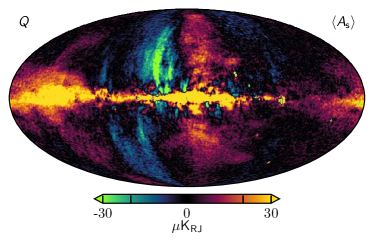
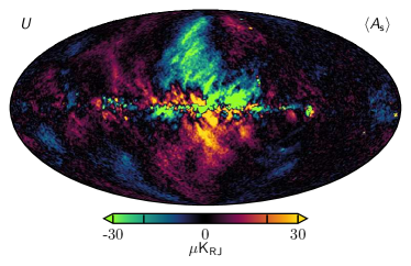
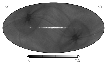
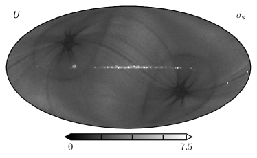
Figure 31: Polarized synchrotron maps and their standard deviations evaluated at 30  GHz.

Figure 27 summarizes the results from these calculations in map domain. Each row corresponds to one DA, while the left and right half-sections of the figure correspond to Stokes $Q$ and $U$, respectively. (One common parameter is fitted per template for both Stokes parameters, but they are for convenience visualized separately.) Within each section, the left column shows the raw difference, the middle column shows the sum of the best-fit templates, and the right column shows the residual obtained after subtracting the best-fit templates from the raw difference.

Comparing the left and middle columns in each section, we see that – at least at a visual level – the WMAP templates do indeed trace the residuals to a high degree for many channels, e.g., K, Q1, V2 etc. For some channels, such as Ka1 and Q2, the agreement is less convincing. However, as seen in the right-most column, even for the well-fitting channels the templates are unable to explain all of the difference.

To roughly estimate how much of the full difference may be described by the WMAP templates, we compute the relative decrease in standard deviation between the full difference map (left columns) and the template-corrected map (right columns) of the form $\sqrt{\sigma_{\mathrm{raw}}^{2}-\sigma_{\mathrm{corr}}^{2}}/\sigma_{\mathrm{raw}}$; in the case that the template correction happened to account for the full difference, this quantity would be unity, while in the case in which it did not account for anything, it would be 0.

The results from this calculation are summarized in the fourth column in Table 5. Here we see that the two linear templates are able to account for between 6 and 52 % of the full large-scale difference between Cosmoglobe and WMAP; the remaining power must either be due to implicit but unmodeled nonlinear couplings between $x_{\mathrm{im}}$ and other parameters, such as the gain, in the WMAP pipeline that are accounted for through the Markov chain sampling in Cosmoglobe; other large-scale systematic effects in WMAP that are unrelated to transmission imbalance; or not-yet-identified systematic uncertainties in Cosmoglobe. Overall, it seems likely that the template-based correction of the low-resolution covariance matrices used in the cosmological WMAP likelihood does not provide a complete description of the full large-scale uncertainties. This could potentially be relevant for the differing estimates of the optical depth of reionization between WMAP9 (Hinshaw et al. 2013) and Planck (Planck Collaboration V 2020), and resolving this point is clearly a high priority for a future second Cosmoglobe data release.

5.4 Comparison with BeyondPlanck LFI frequency maps

Before concluding this section, we briefly compare the updated Cosmoglobe LFI maps with the previous BeyondPlanck products. It is important to keep in mind that whenever new data sets or astrophysical components are added to a global analysis framework such as Cosmoglobe, all frequency channels and astrophysical components are affected by the recent additions. Figure 28 illustrates this in terms of differences between the Cosmoglobe and BeyondPlanck posterior mean maps, all of which are smoothed to a common resolution of $2^{\circ}$ FWHM. No additional postprocessing is performed.

Starting with the temperature case, we see that the color scale spans $\pm 10\thinspace\mu$K. However, most of this range is spent on capturing the monopole component across channels. the monopoles are in general determined by the foreground model, and this is obviously strongly affected by the introduction of the WMAP K-band. The second most important change is a dipole. Specifically, the 30 GHz dipole has changed by 2–3 $\mu$K, and this change is also a direct consequence of the addition of K-band, which now dominates the free-free and AME components. Furthermore, we see that the direction of this dipole is in the opposite direction compared to the CMB Solar dipole, and that the Galactic plane is negative; overall, the absolute calibration of the 30 GHz channel has decreased by about 0.1 %. Also for the 70 GHz we see a dipole difference of about 3–4 $\mu$K, which we will return to the astrophysical implications of in Sect. 6.2.1.

In polarization, we find differences of about 2–3 $\mu$K in the 30 GHz channel, while they are generally below 1 $\mu$K in the 44 and 70 GHz channels. The general morphology of these difference correspond to gain differences, with obvious striping along the Planck scanning path. Thus, this plot serves as yet another powerful demonstration of the tight coupling between gain calibration, temperature component separation, and large-scale polarization systematics.

6 Preliminary astrophysical results

The main scientific goal of the current paper is to derive and publish new low systematic state-of-the-art WMAP frequency sky maps through end-to-end Bayesian analysis. Ideally, these maps should be accompanied with a fully converged posterior distribution that allows derivation of all relevant scientific applications, including low-$\ell$ polarization. However, as discussed in Sect. 3.3, producing a sufficient number of samples for estimating the optical depth of reionization will require about nine months of continuous runtime. At the same time, any scientific applications that do not require such a large number of samples will benefit greatly already from the currently available data.

In this section, we present a number of typical applications for which this is the case. In particular, in Sect. 6.1 we present Galactic foreground maps derived in the current analysis, and in Sect. 6.2 we present WMAP+LFI CMB results, including an updated dipole estimate, a temperature power spectrum, and a reassessment of various low-$\ell$ anomalies. In Sect. 6.3 we quantify the goodness-of-fit of the current Cosmoglobe sky model in terms of frequency residual maps and $\chi^{2}$ statistics, before concluding with a comparison of the relative signal-to-noise ratio of WMAP and LFI to each physical component in Sect. 6.4.

6.1 Galactic foregrounds

As described in Sect. 2.3, and defined by Eqs. (10)–(15), the Galactic sky model we adopt in this analysis is very similar to that of BeyondPlanck (2023). Explicitly, it includes synchrotron, free-free, AME, and thermal dust emission in intensity, and synchrotron and thermal dust emission in polarization, and we fit the individual amplitude of each component per pixel. However, there are two notable changes. First, we adopt an exponential SED model for AME rather than an SpDust-based SED; this is motivated by the observation that the SpDust models appears to underestimate the AME amplitude at frequencies between 40 and 60 GHz. Second, as discussed in Sect. 2.4, we impose stronger (data-informed) priors on the SED parameters. The motivation for this is to reduce degeneracies between the foreground model and overall gains, which otherwise can lead to very long Markov chain correlation lengths. In the future, these priors should be removed after adding additional data that breaks these degeneracies directly, in particular from Planck HFI, QUIJOTE, and C-BASS. As shown in Sect. 6.3, no significant foreground correlated artifacts arise from these priors (as would be the case if the priors were poorly chosen), so these priors have a small impact on the WMAP frequency maps themselves, which are the main scientific targets in this paper. On the other hand, this does imply that the SED parameters that are sampled as part of the Gibbs chain are non-informative. Rather, spectral parameters must be estimated through external analyses from the frequency maps, and this is for instance done for polarized synchrotron emission in a companion paper by Fuskeland et al. (2023).

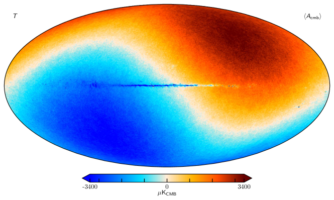
Figure 32: Posterior mean CMB Cosmoglobe temperature map, smoothed to an angular resolution of $14^{\prime}$ FWHM.

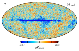
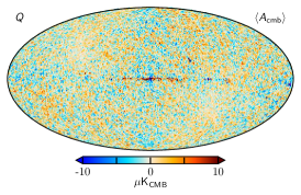
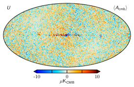
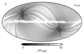
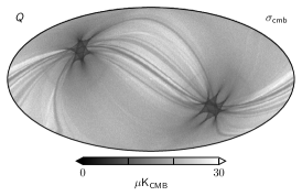
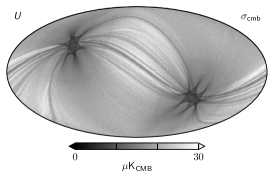
Figure 33: Posterior mean CMB Cosmoglobe maps for Stokes $T$, $Q$, and $U$, and their corresponding standard deviation. The polarization maps have been smoothed to an angular resolution of $2^{\circ}$ FWHM.

Table 6: Comparison of Solar dipole measurements from COBE, WMAP, and Planck.

     Galactic coordinates      Amplitude      $$l b [\thinspace\mu {}_{\rm CMB}] 3358\kern 2.22223pt\kern 4.00002pt\kern 4.00002pt\pm 23\kern 2.22223pt\kern 4.00002pt\kern 4.00002pt 264.31\kern 4.00002pt\pm 0.16\kern 4.00002pt 48.05\kern 4.00002pt\pm 0.09\kern 4.00002pt 3355\kern 2.22223pt\kern 4.00002pt\kern 4.00002pt\pm\kern 4.00002pt8\kern 2.22223pt\kern 4.00002pt\kern 4.00002pt 263.99\kern 4.00002pt\pm 0.14\kern 4.00002pt 48.26\kern 4.00002pt\pm 0.03\kern 4.00002pt 3365.5\kern 4.00002pt\pm\kern 4.00002pt3.0\kern 4.00002pt 264.01\kern 4.00002pt\pm 0.05\kern 4.00002pt 48.26\kern 4.00002pt\pm 0.02\kern 4.00002pt 3364.29\pm\kern 4.00002pt1.1\kern 4.00002pt 263.914\pm 0.013 48.265\pm 0.002 3364.4\kern 4.00002pt\pm\kern 4.00002pt3.1\kern 4.00002pt 263.998\pm 0.051 48.265\pm 0.015 3362.08\pm\kern 4.00002pt0.99 264.021\pm 0.011 48.253\pm 0.005 3361.90\pm\kern 4.00002pt0.40 263.959\pm 0.019 48.260\pm 0.008 3366.6\kern 4.00002pt\pm\kern 4.00002pt2.6\kern 4.00002pt 263.986\pm 0.035 48.247\pm 0.023 3362.7\kern 4.00002pt\pm\kern 4.00002pt1.4\kern 4.00002pt 264.11\kern 4.00002pt\pm 0.07\kern 4.00002pt 48.279\pm 0.026 \bf 3366.2\kern 4.00002pt\pm\kern 4.00002pt1.4\kern 4.00002pt \bf 264.08\kern 4.00002pt\pm 0.07\kern 4.00002pt \bf 48.273\pm 0.024$$       Experiment      K      [deg]      [deg]      Reference COBE^a,b.                        Lineweaver et al. (1996) WMAP ^c.                        Hinshaw et al. (2009) LFI 2015 ^b.                        Planck Collaboration II (2016) HFI 2015 ^d.                        Planck Collaboration VIII (2016) LFI 2018 ^b.                        Planck Collaboration II (2020) HFI 2018 ^d.                        Planck Collaboration III (2020) Bware .                        Delouis et al. (2021) Planck PR4 ^a,c.                        Planck Collaboration Int. LVII (2020) BeyondPlanck ^e .                        Colombo et al. (2023) Cosmoglobe ^e .                        This work

^aStatistical and systematic uncertainty estimates are added in quadrature.

^bComputed with a naive dipole estimator that does not account for higher-order CMB fluctuations.

^cComputed with a Wiener-filter estimator that estimates, and marginalizes over, higher-order CMB fluctuations jointly with the dipole.

^dHigher-order fluctuations as estimated by subtracting a dipole-adjusted CMB-fluctuation map from frequency maps prior to dipole evaluation.

^eEstimated with a sky fraction of 68 %. Error bars include only statistical uncertainties, as defined by the global Cosmoglobe posterior framework, and they thus account for instrumental noise, gain fluctuations, parametric foreground variations etc.

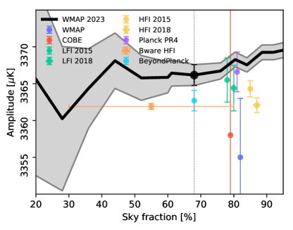
Figure 34: CMB dipole amplitude as a function of sky fraction. The gray band indicates the 68 % posterior confidence region.

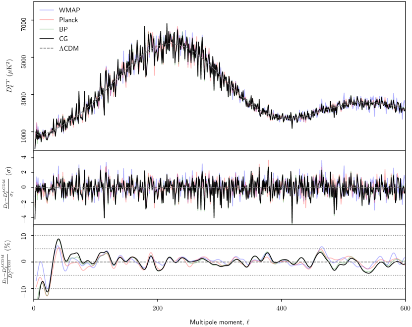
Figure 35: (Top:) Angular CMB temperature power spectrum, $D_{\ell}^{\mathrm{TT}}$, as derived by Cosmoglobe (black), BeyondPlanck (green), Planck (red), and WMAP9 (blue). The best-fit Planck 2018 $\Lambda$CDM spectrum is showed in dashed gray. (Middle:) Residual power spectrum relative to $\Lambda$CDM, measured relative to the quoted error bars, $(D_{\ell}-D_{\ell}^{\mathrm{\Lambda CDM}})/\sigma_{\ell}$. For pipelines that report asymmetric error bars, $\sigma_{\ell}$ is taken to be the average of the upper and lower error bar. (Bottom:) Fractional difference with respect to the Planck $\Lambda$CDM spectrum. In this panel, each curve has been boxcar averaged with a window of $\Delta\ell=100$ to suppress random fluctuations.

In this section, we therefore focus only on the foreground amplitude parameters. Specifically, Fig. 29 shows posterior mean intensity maps for all four components, while Fig. 31 shows the posterior mean and standard deviation for the polarized synchrotron component.

Starting with the free-free intensity component shown in the top left panel of Fig. 29, we observe good agreement with previous full sky component separation studies (Planck Collaboration X 2016; Andersen et al. 2023). We note that compared to the Planck Collaboration X (2016) analysis, there is less diffuse structure in the free-free component, which is driven by the imposition of a prior on the component amplitude at high Galactic latitudes (Andersen et al. 2023). However, in high emission regions, such as the Galactic plane and the Gum Nebula, we see good agreement.

For the AME, shown in the top right panel, we see a slightly differing morphology compared to both Planck Collaboration X (2016) and Andersen et al. (2023). The most notable difference is the lack of extended diffuse structure in this work, with a marginal shift in the overall direction of the component’s dipole. These differences are due to the different SED model, as well as the degeneracy between the K-band gain and the AME dipole, as described at length in Sect. 7.3. Both this analysis and Andersen et al. (2023) differ from the Planck Collaboration X (2016) AME solution by showing less extended diffuse structure, and most visibly notable is the $\rho$-Ophiuchi complex, which appears as a hole in the AME component in this work. For further details regarding the AME SED, we refer the interested reader to Watts et al. (2023a).

Next, regarding synchrotron emission in total intensity, the reprocessed full sky Haslam map (Remazeilles et al. 2015) at 408 MHz is used as an anchor for the full sky synchrotron emission in both Planck 2015, BeyondPlanck, and Cosmoglobe. As such, the estimate shown in the bottom right panel of Fig. 29 shares very similar morphology to both these previous analyses, although there are some slight deviations around point sources. Similar observations apply to the thermal dust model, which is strongly dominated by the Planck 857 GHz, which is common to all these mentioned analyses.

Though the BeyondPlanck analysis did not utilize the WMAP K-band, the foreground model derived in Andersen et al. (2023) still predicted the sky model at K-band. As such, it is therefore interesting to check how well the BeyondPlanck model was able to predict the current K-band signal. To this end, we compare the AME-plus-free-free contribution at 22  GHz between this work and the sky model derived in BeyondPlanck. (Synchrotron and thermal dust emission is omitted in this particular calculation since these are strongly dominated by the same data sets in the two analyses, namely Haslam 408 MHz and Planck 857 GHz.) The combined sky model, smoothed to $2^{\circ}$, is shown as a fractional difference $\Delta A_{\mathrm{K}}=s^{\mathrm{CG}}_{\mathrm{AME}+\mathrm{ff}}-s^{\mathrm{BP}}_{\mathrm{AME}+\mathrm{ff}})/s^{\mathrm{BP}}_{\mathrm{AME}+\mathrm{ff}}$ in Fig. 30. Here we see that the addition of K-band data has altered the sky model at 22 GHz in the high-signal-to-noise region by 5–10 %, and the new model exhibits a stronger foreground amplitude at 22 GHz than the BeyondPlanck model. Detailed inspection of the individual free-free and AME components indicate that they have typically changed by about 20 %, which is also partially due to the exponential SED model used for AME in the present analysis.

Finally, for the polarized synchrotron amplitude, shown in Fig. 31, we also find good agreement with previous BeyondPlanck results (Svalheim et al. 2023b). However, the morphology of the standard deviation map shows a stronger imprint of the WMAP scanning strategy than in BeyondPlanck, because the K-band data were omitted from that analysis. In this updated work, the two experiments have more comparable signal-to-noise ratios to polarized synchrotron emission, and which experiment is stronger depends now on position on the sky. As a result of finally combining all WMAP and LFI data, this updated map represents the most sensitive full-sky polarized synchrotron map published to date.

6.2 CMB results

Next, we consider various CMB results, the most important scientific products from both WMAP and Planck. In this paper, we focus primarily on intensity results, as far fewer Markov chain samples are required to produce robust results for these than large-scale polarization. In addition, cosmological parameter estimation is also left for future work, simply because we find that the angular temperature power spectrum derived in this work is fully consistent with that derived in BeyondPlanck, and no significant changes are therefore expected. Once a robust low-$\ell$ polarization likelihood has been established, this issue will of course be revisited.

Figure 32 shows the posterior mean CMB intensity map including the dipole, while Fig. 33 shows the posterior mean and standard deviation for all three Stokes parameters; in this figure, the best-fit CMB Solar dipole has been subtracted from the temperature map. Overall, these maps look visually very similar to those presented by BeyondPlanck (Andersen et al. 2023), and we therefore adopt the same confidence masks and analysis configuration as described there.

6.2.1 Solar dipole

We start our discussion with the largest angular scales, namely the CMB dipole. As discussed by Thommesen et al. (2020), estimating the Solar dipole is arguably one of the most difficult parameters to constrain accurately. This is due to the strong degeneracy with the gain model, as well as the effect of mode coupling when masking the Galactic plane. Calibration misestimation propagates directly into an incorrect CMB dipole, and vice-versa.

Our Solar dipole estimates are summarized in Table 6 and Fig. 34. First, we find that the dipole direction is very consistent with BeyondPlanck (Colombo et al. 2023), and also statistically consistent with most previous analyses within the quoted uncertainties. Strong agreement with BeyondPlanck is of course expected, since the data selection is very similar (the only difference is that K-band has been added in Cosmoglobe), and the processing pipelines are very similar.

It is therefore interesting to note that the dipole amplitude is in fact 3.5 $\mu$K (or $2.5\thinspace\sigma$) higher than in BeyondPlanck. This is clearly a larger change than one would expect simply by adding one more data set. It is also interesting to note that this new mean value of 3366.2 $\mu$K is $11\thinspace\mathrm{\mu K}$ higher than the WMAP9 result (Hinshaw et al. 2009), and also 4.1 $\mu$K higher than the Planck HFI 2018 result (Planck Collaboration II 2020). On the other hand, it is now consistent with the latest Planck PR4 result, with a difference of only 0.4 $\mu$K.

One plausible explanation for this behaviour is the following: BeyondPlanck used the official WMAP9 frequency maps directly in the analysis, and these data are known to have a lower CMB dipole than Planck. It is therefore natural to assume that the BeyondPlanck dipole was pulled toward low values by these maps. In the new Cosmoglobe analysis, however, the WMAP and Planck data are forced to agree on a common dipole prior during the global calibration process. In particular, this has increased the WMAP dipole, and the previous tension has been released. The net result is that the WMAP+LFI-dominated Cosmoglobe estimate now finally agree with the highly independent Planck HFI-dominated PR4 result.

6.2.2 Angular temperature power spectrum

Next, in Fig. 35 we show the angular temperature power spectrum derived from the CMB samples from the main Gibbs chain, obtained using a Gaussianized Blackwell-Rao estimator (Chu et al. 2005; Rudjord et al. 2009) with an identical analysis setup and mask as in BeyondPlanck (Colombo et al. 2023). We compare with the official WMAP (Hinshaw et al. 2013) and Planck (Planck Collaboration V 2020) power spectra, as well as the BeyondPlanck (Colombo et al. 2023) spectrum. For reference, the best-fit Planck 2018 $\Lambda$CDM spectrum is also plotted along side them. The middle panel shows the deviation from the Planck $\Lambda$CDM solution, in units of $\sigma_{\ell}$ from each individual pipeline, while the bottom panel shows the fractional difference with respect to the Planck $\Lambda$CDM spectrum.

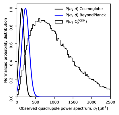
Figure 36: Temperature quadrupole power amplitude posterior distribution as computed by Cosmoglobe (solid black line) and BeyondPlanck (solid blue line). For comparison, the histogram shows 100 000 realizations of $\sigma_{2}$ given the best-fit Planck 2018 ensemble-averaged prediction of ${C_{2}^{\Lambda\mathrm{CDM}}=1064.7\thinspace\mathrm{\mu K^{2}}}$.

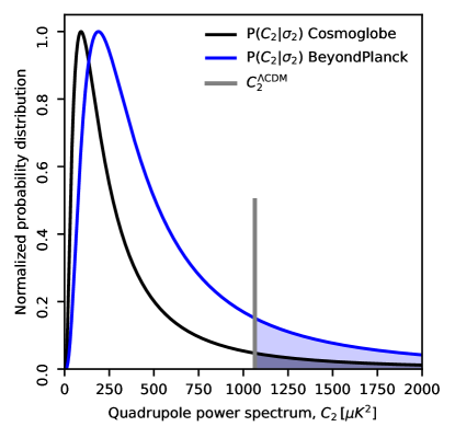
Figure 37: Marginal probability distribution of the ensemble-averaged $C_{2}$ given the data, $P(C_{2}\mid\@vec{d})$, as measured by Cosmoglobe (black) and BeyondPlanck (blue).

At $\ell\lesssim 500$, each of these datasets are signal-dominated, and all spectra agree very well. At higher multipoles, more samples are needed in order to obtain a robust Blackwell-Rao estimator. Given this good agreement, we do not anticipate any significant difference in terms of $\Lambda$CDM parameters, and we therefore postpone a full cosmological parameter reanalysis to future work.

6.2.3 Low-$\ell$ anomalies

Although the CMB power spectrum agrees exceedingly well with a $\Lambda$CDM model (e.g., Hinshaw et al. 2013; Planck Collaboration VI 2020; Paradiso et al. 2023), several anomalies have been reported that appear to be in tension with this model, in particular on large angular scales (e.g., Planck Collaboration VII 2020, and references therein). Generally, the presence of these anomalies in the CMB map is not debated as such; however, their statistical significances are highly debated. In particular, some authors argue that the correct interpretation of these anomalies are likely to be described by the so called look-elsewhere effect (e.g., Bennett et al. 2011).

The traditional approach to studying CMB anomalies is to compute a single maximum-likelihood CMB map and a corresponding ensemble of $\Lambda$CDM simulations processed with similar instrumental properties. Then one derives a single value for a given anomaly statistic of interest, and compares the true value with the histogram of simulated values. By counting how many simulations exceed the true value, one obtains a probability-to-exceed (PTE) value that quantifies the level of agreement.

In our case, however, we do not have only a single best-fit CMB likelihood map, but rather a full posterior distribution of such maps produced through the Gibbs chain. These can then be used to assess the significance of any given anomaly using exactly the same approach as in a traditional analysis, except that one now obtains a histogram for the real data as well. The main advantage of this approach is that systematic uncertainties are propagated with much greater fidelity than with a single maximum-likelihood map. This is particularly important for very low-$\ell$ anomalies, which tend to be sensitive to the instrument calibration, and propagating these uncertainties properly is nontrivial using traditional approaches (Brilenkov et al. 2023).

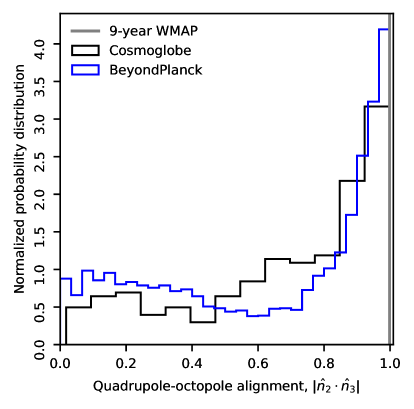
Figure 38: The quadrupole-octopole alignment of Cosmoglobe compared with BeyondPlanck and 9-year WMAP.

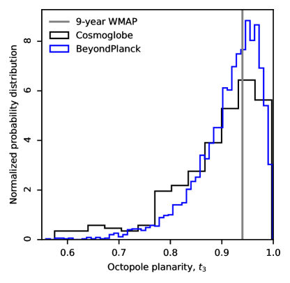
Figure 39: The octopole planarity statistics $t_{3}$ compared with the BeyondPlanck analysis (blue).

In this section, we revisit a few well known low-$\ell$ anomalies regarding the two lowest multipoles, $\ell=2$ and 3, and compare our findings with similar results reported by BeyondPlanck (Colombo et al. 2023). The main difference between these two analyses is thus that the WMAP data are now analyzed in time domain, rather than in the form of preprocessed maps. It is reasonable to assume that this recalibration can modify the amplitude and morphology of these lowest multipoles, in particular given the notable differences in the CMB dipole amplitude reported in Sect. 6.2.1.

First, we start with the absolute amplitude of the temperature quadrupole, which has been noted to be low compared to the theoretical prediction ever since COBE-DMR (Bennett et al. 1992). This was later confirmed by both WMAP (Hinshaw et al. 2003) and Planck (Planck Collaboration Int. XV 2014), but with large discrepancies in mean value and error bars, both within and between experiments (Colombo et al. 2023). For instance, the WMAP team reported in their 7-year analysis a best-fit value of $201\thinspace\mu\mathrm{K}^{2}$ (Larson et al. 2011), which decreased to $151\thinspace\mu\mathrm{K}^{2}$ in the 9-year analysis (Hinshaw et al. 2013). The naive Fisher uncertainty on $\sigma_{2}$ was reported by Hinshaw et al. (2013) to be $9\thinspace\mu\mathrm{K}^{2}$ which only accounted for a noise-only estimate. As such, this relative change between the two algorithmically very similar 7- and 9-year analyses corresponded to a roughly $5\leavevmode\nobreak\ \sigma$ discrepancy in terms of Fisher uncertainties. Similarly, Planck later found in 2013 and 2018 $\sigma_{2}$ to be 299 and 226 $\mu\mathrm{K}^{2}$, respectively, which corresponds to an internal $8\thinspace\sigma$ discrepancies in terms of Fisher uncertainties (Planck Collaboration V 2020).

These large variations indicate that instrumental noise is not the dominant source of uncertainty regarding $\sigma_{2}$. Indeed, this observation was demonstrated in practice through the end-to-end BeyondPlanck analysis, which found an amplitude of $229\pm 97\thinspace\mu$K². The important point about this estimate is that the uncertainty is almost an order of magnitude larger than the Fisher uncertainty, and this is likely driven by the additional marginalization over calibration uncertainties.

With the new set of Cosmoglobe CMB maps derived in this paper, we are in a position that allows us to improve further on the BeyondPlanck result, by additionally marginalizing over WMAP instrumental effects. This is quantified in terms of the marginal posterior distribution, $P(\sigma_{2}\thinspace|\thinspace\@vec{d})$, which is shown in Fig. 36. The Cosmoglobe estimate may be summarized in terms of a Gaussian distribution with $\sigma_{2}=131\pm 69\ \mu\mathrm{K}^{2}$. For comparison, the corresponding BeyondPlanck result is plotted as a blue curve in the same figure, while the histogram shows $10^{5}$ realizations of $\sigma_{2}$ given the Planck 2018 best-fit $C^{\Lambda\mathrm{CDM}}_{2}=1064.6\thinspace\mu\mathrm{K}^{2}$ (Planck Collaboration VI 2020). It is interesting to note that this updated central value is almost a factor of two lower than the previous BeyondPlanck results, which suggests that the largest scales have indeed changed sufficiently in the updated WMAP to affect the low-$\ell$ anomalies. Furthermore, the low quadrupole amplitude anomaly has become more anomalous through these modifications, and is now almost as low as the 1-year WMAP result.

To quantify the statistical significance of the low $\sigma_{2}$ value, we first compute the probability of obtaining an ensemble-averaged power coefficient, $C_{2}$, equal to or larger than the $\Lambda$CDM prediction given the observed realization-specific power coefficient, $\sigma_{2}$. This can be done by evaluating full marginal posterior distribution $P(C_{2}\mid\sigma_{2})$ as a function of $C_{2}$ through the Blackwell-Rao estimator (Chu et al. 2005). This is shown as a solid black line in Fig. 37, while the solid blue line shows the corresponding BeyondPlanck result; the vertical gray line shows the Planck best-fit value of $C^{\Lambda\mathrm{CDM}}_{2}=1064.6\thinspace\mu\mathrm{K}^{2}$. Computing the integrals above this value, we find that the probability for $C_{2}$ to exceed $C^{\Lambda\mathrm{CDM}}_{2}$ is $11.0\thinspace\%$ for Cosmoglobe and $21.7\thinspace\%$ for BeyondPlanck, both indicated as shaded areas.

Next, in Fig. 38 we revisit the so-called quadrupole-octopole alignment statistic, $|\hat{n}_{2}\cdot\hat{n}_{3}|$, introduced by de Oliveira-Costa et al. (2004). This statistic quantifies the angular distance between the vectors that maximize the angular momentum of each multipole, and is thus a measure of the relative alignment between the plane of these modes on the sky. Again, the black line shows the posterior distribution derived from the Cosmoglobe samples, while the blue histogram shows the same for BeyondPlanck; the vertical gray line shows the best-fit value derived from WMAP9 data. Our updated results are fully consistent with those reported by Colombo et al. (2023) for BeyondPlanck; while the new results that implement full end-to-end error propagation are statistically consistent with the classical pipelines in terms of a single best-fit value, the total posterior uncertainty is now much larger, both because of marginalization over a more complete instrumental model and a more conservative confidence mask (Colombo et al. 2023), to the point that the evidence for this effect is no longer compelling.

Figure 39 shows similar result for the octopole planarity statistic, also introduced by de Oliveira-Costa et al. (2004). As for BeyondPlanck, we also in this case observe a broad distribution of allowed values, and the Cosmoglobe distribution is even a little broader than the BeyondPlanck distribution; this is of course expected, since we now marginalize over a larger set of instrumental parameters. At the same time, it is intriguing to note that the maximum posterior value is actually even closer to one in Cosmoglobe than in WMAP9, which indicates that it is in fact possible to attribute all the octopole power into one single azimuthal mode, $a_{33}$. In order to shed more light on this effect, the overall error budget must be decreased significantly by adding more data, in particular Planck HFI observations.

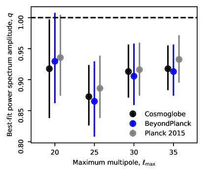
Figure 40: Best-fit amplitude, $q$, of the low multipole power spectrum $C_{\ell}=qC^{\Lambda\mathrm{CDM}}_{\ell}$, $2\leq\ell\leq\ell_{\mathrm{max}}$ compared to Planck 2015 (grey) and BeyondPlanck (blue).

Finally, Fig. 40 provides an update of the so called low multipole power anomaly first presented by Planck Collaboration XI (2016). In this case, we fit a scaling factor, $q$, relative to the $\Lambda$CDM spectrum to multipoles between $2\leq\ell\leq\ell_{\mathrm{max}}$, and vary $\ell_{\mathrm{max}}$ between 20 and 35. In this figure, we see that the low-$\ell$ power increases very slightly from BeyondPlanck to Cosmoglobe, and it is now even closer to Planck 2015. Overall, the significance of this effect is similar to previously reported results.

6.3 Goodness-of-fit: Map-level residuals and $\chi^{2}$ statistics

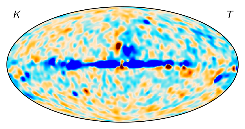
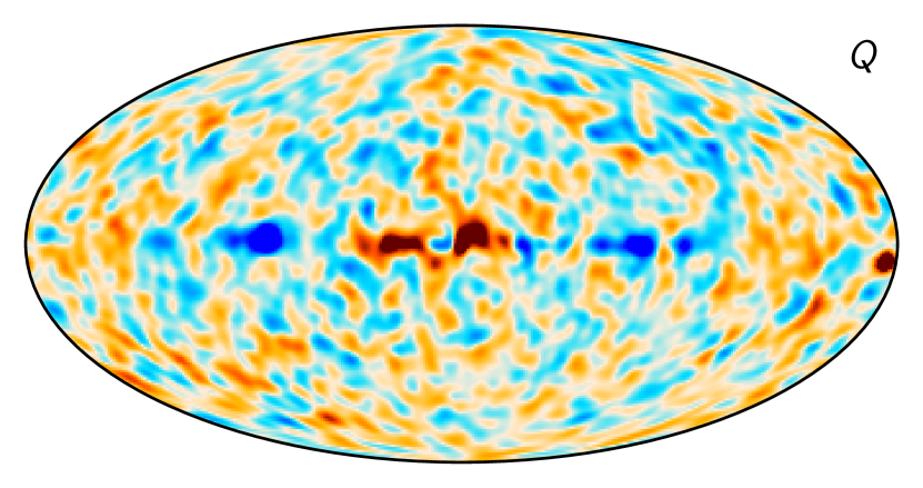
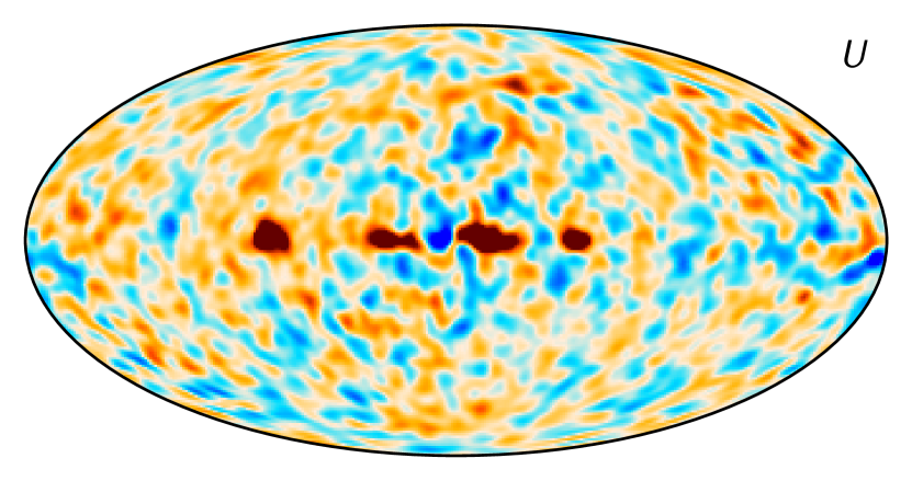
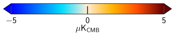
Figure 41: Frequency map residual (DA map minus sky model) for K-band. Panels show, from top to bottom, Stokes $T$, $Q$, and $U$, and all maps are smoothed by $5^{\circ}$ FWHM.

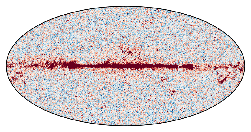
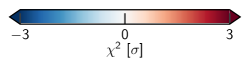
Figure 42: Pixel-space reduced normalized $\chi^{2}$. In this figure, $n_{\mathrm{dof}}=300$, which is obtained from fitting to the regions outside of the K-band processing mask; for further information regarding this statistic, see Andersen et al. (2023).

The quality of the component separation procedure is evaluated through map space residuals (i.e., frequency map minus sky model) and a spatial map of the reduced $\chi^{2}$. Residual maps for all three K-band Stokes parameters are shown in Fig. 41, while Fig. 61 in Appendix B shows the same for all DAs. Figure 42 shows the total reduced normalized $\chi^{2}$, summed over all frequency channels. Overall, we see that the magnitude of the map level residuals are generally well below 5 $\mu$K, and the morphology at high Galactic latitudes are generally consistent with instrumental noise. However, in intensity, the Galactic plane stands out with statistically significant residuals, in particular at the Galactic center and bright regions such as the Orion region, $\rho$ Ophiuchus, and the Large Magellanic Cloud. Implementing support for a more complex and realistic foreground model, and therefore necessarily also adding support for additional datasets, is an important goal of the general Cosmoglobe framework, and this will hopefully reduce these residuals in the future. In particular, integrating the Planck HFI data, and thereby being able to fit thermal dust emission pixel-by-pixel represents a key milestone in this program.

Inspecting the residual maps for all channels in Fig. 61, we first of all see that the polarization maps are generally consistent with instrumental noise at all channels. This is even true for the W-band, although in this case the impact of correlated noise (due to its higher $f_{\mathrm{knee}}$ parameter) is clearly evident. In temperature, the situation is less clear, as there are weak large-scale residuals at the $\sim$ 2 $\mu$K level present in most channels, but with different morphologies in each case. Clearly, these residuals indicate the presence of some very low-level residual systematics that have not been perfectly modeled in the current processing. Considering the spatial structure of these residuals, it is natural to suspect the small non-idealities in the gain or baseline model; this seems particularly plausible given the pronounced annual temperature variations seen in Figs. A and 49. Of course, considering that the amplitude of these residuals is indeed very low compared to the overall sky signal, they are not likely to have any significant impact on any cosmological or astrophysical residuals, but they should nevertheless be understood through future work in order to reach the full white-noise potential of the experiment.

6.4 WMAP and LFI signal-to-noise ratio comparison

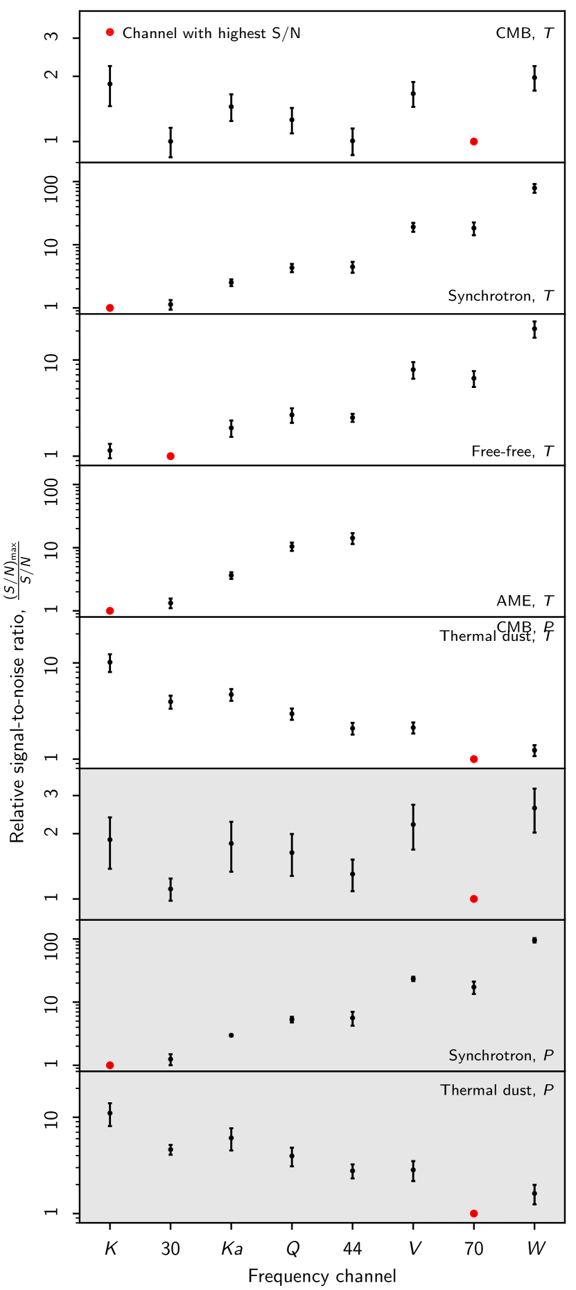
Figure 43: Relative signal-to-noise ratios for WMAP and LFI channels and various components, as defined in terms of the ratio between the mixing matrix and the total instrumental uncertainty, $\psi=\@tens{M}/\sigma$. The total instrumental uncertainty is derived by adding the white noise and instrumental uncertainty maps (as given by Figs. 56 and 57) in quadrature. Values are reported as the ratio between the most sensitive channel (marked by a red dot) and the given channel; points with error bars correspond to mean and standard deviations evaluated over the full sky. Panels with white background indicate intensity results, while panels with gray background indicates polarization results. All quantities are evaluated at a common angular resolution of $2^{\circ}$ FWHM.

We conclude this section with a comparison of the relative signal-to-noise ratios to each astrophysical component between WMAP and Planck LFI. To quantify this, we first define the normalized signal-to-noise ratio for a given channel $\nu$ and pixel $p$ to be the ratio between the mixing matrix and the total noise rms, $\psi\equiv M_{c}(\nu,p)/\sigma(\nu,p)$, all evaluated at a common angular resolution of $2^{\circ}$ FWHM. The total noise level is estimated by adding in quadrature the white noise and posterior rms levels, similar to those shown in Figs. 56 and 57 but both evaluated at $2^{\circ}$ FWHM. We then identify the channel with the highest mean value of $\psi$ for a given component, and adopt this as a reference channel. Finally, we compute $r=\psi_{\mathrm{max}}(p)/\psi(p)$ for all pixels,and report the mean and standard deviation over the full sky.

The results from this calculation are summarized in Fig. 43 for all WMAP and LFI channels. The top five panels (with white background) show temperature results, while the bottom three panels (with gray background) show polarization results. In each case, the red dot indicates the reference channel with highest signal-to-noise ratio, which by definition has value equal to one. For a given other channel, $X$, the values in Fig. 43 should be interpreted as “The reference channel has $r$ times higher signal-to-noise ratio with respect to component $c$ than channel $X$.”

Starting from the CMB intensity case shown in the top panel, we first note that both LFI and WMAP internally have fairly similar signal-to-noise ratio, in agreement with their design specifications. Furthermore, we see that each of the LFI channels generally is about 1.5–2 times more sensitive that each of the WMAP channels, and taking into account the fact that WMAP has five channels, while LFI only has three, the total raw sensitivity of the two experiments is therefore quite comparable. This, in combination with the inter-leaved center frequencies, make the two experiments highly complementary.

Next, the second panel shows the results for synchrotron emission in intensity. Since the synchrotron SED scales roughly as $\mathcal{O}(\nu^{-3})$, K-band is the overall strongest synchrotron tracer, although the LFI 30 GHz is lower only by about 13 %. A similar observation is true also for AME, while for free-free emission LFI 30 GHz is about 15,% more sensitive than K-band. In contrast, the Planck 70 GHz channel is strongest with respect to thermal dust emission, and it is about 23 % more sensitive than W-band and two times more sensitive than V-band.

Finally, we see very similar behaviour in polarization. The LFI 70 GHz channel is strongest for both CMB and thermal dust emission, while for polarized synchrotron emission, K-band is stronger than LFI 30 GHz by about 25 %. Again, we note that all these calculations refer to an angular resolution of $2^{\circ}$ FWHM, and the results will vary with angular scale due to the different angular resolutions of the two experiments.

7 Outstanding issues

As shown in the previous sections, there are very few residuals, artifacts, or systematics within this jointly processed dataset, hereafter referred to as Cosmoglobe data release 1 (CG1). However, the global nature of this analysis allows us to identify issues in the data processing that will otherwise have gone unnoticed. In this section, we enumerate the issues we have encountered in CG1, and which we plan to improve upon in future data releases.

7.1 Noise modeling

As discussed in Sect. 4.4, and shown explicitly in Fig. 54, the TOD-level $\chi^{2}$ is discrepant up to the $10\sigma$ level for several WMAP diodes. The main driver of this model failure lies in the fact that our current noise estimation algorithm fits the white noise level by computing the standard deviation of pairwise signal-subtracted sample differences. The motivation for this is to prevent slowly varying model failures from contaminating the white level, which worked very well for Planck LFI (Ihle et al. 2023). However, the WMAP time-ordered data exhibits a low level of colored noise at very high temporal frequencies, and is not supported by a rigid $1/f$ model. This is illustrated in Fig. 10, which shows that the high-frequency noise is fixed to the noise PSD at the sampling frequency. In contrast, if $\sigma_{0}$ were a free parameter in this particular parametric fit, it would be driven by the intermediate frequencies 2–6 Hz at the expense of a good fit at the highest frequencies.

The particular case of W413’s PSD is a noise spectrum that could easily be modeled as a spectrum that is continuing to drop beyond the sampling rate, not dissimilar to the two-pole Bessel filter implemented in WMAP’s electronics (Jarosik et al. 2003b). In practice, the white noise can be identified with the flat portion of the spectrum well above $f_{\mathrm{knee}}$, but in the case of these noise spectra, there is no such flat portion, challenging the very existence of “white noise” for this particular diode. Additionally, a Bessel filter tail could affect the signal band as well, requiring more detailed modeling of the noise.

In practice, the decomposition of instrumental noise into a “white” component and a correlated component is very useful, and provides a stringent test for the final data products. Indeed, the particular model failure was so subtle that such a description of noise being split into scale-dependent and scale-independent would have made it nearly impossible to detect such an issue. For the case of WMAP data, there is a natural need to improve the noise PSD modeling, especially when a successful parametrization was found by the WMAP team in time space. In practice, this will likely be useful for the analysis of other CMB experiments, and will be of broad use in the future.

An additional issue is that of correlation between pairs of diodes. In general, the correlation between a diode pair is close to 5 %, but for some radiometers the correlation is up to 25 %. In Fig. 44, we plot an example of this, showing the correlation between the TOD residuals in a single scan for W2. In this case, the correlation between diodes within W21 is ${\sim 20\thinspace\%}$, compared to $\sim 0.01\thinspace\%$ for diodes corresponding to different radiometers, i.e., W213 and W224. Explicitly modeling this effect will be an important step for future data releases, both as a goal in itself, but also for developing the tools for future high-precision $B$-mode searches from, e.g., LiteBIRD.

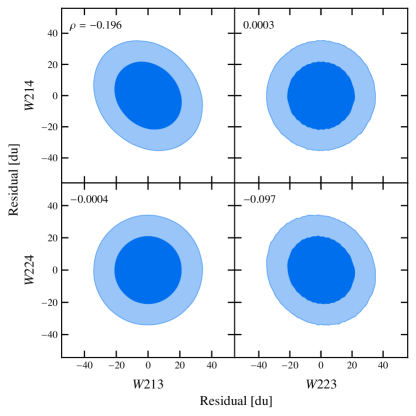
Figure 44: Pearson correlation coefficients between diode residuals for data spanning MJDs 55355.75–55358.24. This estimates the amount of correlated noise shared between detectors.

7.2 Large-scale intensity residuals

As shown in the residual maps in Fig. 61, we identify large-scale residuals at the level of 1–2 $\mu$K in intensity in all DA maps. The detailed morphology of these residuals vary from channel to channel, and it is difficult to pinpoint their origin to a given physical effect. However, due to their long-range coherence, it is natural to speculate that they are associated with either the gain or baseline model. In this respect, it is worth recalling that while the WMAP gain model includes gain fluctuations on all time-scales down to 23 sec, as constrained by housekeeping data, the Cosmoglobe gain model is constant within each scan, and the durations of these are several days. While the overall improvement in large-scale consistency in Cosmoglobe strongly suggests that gain fluctuations on time-scales of minutes or hours cannot be large, they could potentially be relevant for residuals at the 1–2 $\mu$K level. It might therefore be useful in future work to integrate housekeeping data also in Cosmoglobe; if not with a resolution of 23 sec, then perhaps smoothed to minutes or hours.

A similar issue was discovered by Jarosik et al. (2007) in the form of an $8\thinspace\mathrm{\mu K}$ dipole, and this was determined to be due to an inadequacy in the gain model. As mentioned earlier, we assume a linear baseline trend throughout a given scan, and allow correlated noise residuals to pick up longer scale fluctuations. Compared to the WMAP team’s approach of fitting cubic polynomials every hour, there is much more room for unmodeled temporal variation in zero-level. As the gain, correlated noise, and baseline are all deeply correlated, a subtle error in the baseline determination could easily induce a small quadrupolar signal.

It is also worth noting that in an early stage of this analysis, a large quadrupolar signal was induced due to an error in the orbital dipole calculation. Essentially, a single satellite velocity was assumed for an entire scan, which proved to be a poor approximation over $\sim$$3$-day period. A linear interpolation between scans improved this issue, and a cubic interpolation provided a negligible improvement. This observation points generally to a strong correlation between long-timescale effects and quadrupolar residuals. In particular, if one assumes that a given unmodelled systematic error can generate any type of large-scale pattern, then the dipole component of that pattern can typically be mostly accommodated for in the model as a gain or sky signal dipole variation. Spurious quadrupoles, on the other hand, are much harder to account for in our parametric model, and the leading modes in both residual and channel difference maps therefore often take a quadrupolar shape; this is indeed seen in Figs. 19 and 61.

7.3 Degeneracy between K-band calibration and AME dipole

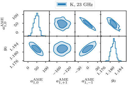
Figure 45: Correlation between K-band’s absolute calibration $g_{0}$ [$\mathrm{du\thinspace mK^{-1}}$] and AME dipole’s spherical harmonic coefficients [$\mathrm{\mu K_{RJ}}$].

As discussed in Sect. 2.4, we have identified a strong degeneracy between K-band’s absolute calibration and the AME dipole that requires external information to break. In this work, we implemented a prior on the absolute calibration based on its effect on the AME dipole. To illustrate this degeneracy, we can compare the absolute K-band calibration with the AME dipole values in terms of the posterior distribution, a slice of which is shown in Fig. 45. Here the degeneracy between $g_{0}$, $a_{1,0}^{\mathrm{AME}}$, and $g_{1,-1}^{\mathrm{AME}}$ is quite apparent. Because there is no causal connection between $g_{0}$ and the AME dipole, we apply a prior the analysis in this work that results in a physically plausible AME dipole.

In the official WMAP pipeline, the degeneracy was effectively broken by using a preliminary K-band sky map and removing it from the timestream. In practice, both solutions are the result of scientific intuition solving an algorithmic issue. The Cosmoglobe approach of using a prior on $g_{0}$ comes from the strong prior that Galactic emission should not have a dipole aligned with the CMB’s Solar dipole. The WMAP team’s approach of using a previous iteration’s map as a sky model comes from the strong prior that errors in the first iteration of the sky map are uncorrelated with the orbital dipole in the timestream.

Even though the Cosmoglobe K-band absolute calibration is informed by the requirement of obtaining a physically reasonable AME dipole, the resulting instrumental solution still generates maps that are consistent with the sky model at the $1\thinspace\mathrm{\mu K}$ level at high Galactic latitudes. Conversely, the WMAP9 solution does not rely on any knowledge of the sky, but as a result induces poorly measured modes with a $2.5\thinspace\mathrm{\mu K}$ amplitude.

Regardless of the details, an accurate model of the sky as observed by the K-band is a necessary condition for obtaining an accurate measurement of the gain. The difficulty of obtaining an accurate AME model is of course compounded by the fact that the AME is brighter in K-band than any of the other WMAP or Planck bands. This may be mitigated in the near future, following a joint WMAP+LFI+QUIJOTE analysis, but this of course depends on the signal-to-noise of AME in QUIJOTE’s frequencies, and is further hindered by QUIJOTE’s partial sky coverage. Relatedly, also the introduction of Planck HFI data may help breaking this degeneracy by providing much stronger constraints on CMB and free-free emission, both of which are significantly degenerate with AME for the current data selection (Andersen et al. 2023).

A future analysis involving the most robust parts of the WMAP9 and Cosmoglobe analysis also has the potential to solve the $g_{0}$-AME degeneracy. In particular, as noted above, the Cosmoglobe analysis did not directly use the housekeeping data to estimate the gain model. There is no a priori reason that the parameters in Eq. (49) cannot be included in the Gibbs chain. This would of course require detailed knowledge of the WMAP satellite’s hardware, and we hope that a joint effort between the WMAP team and Cosmoglobe will help to solve this outstanding issue.

7.4 Other minor effects

The issues listed above are known problems in the analysis that will be fixed in the future. Below, we discuss parts of the analyses that we know exist, but have not yet made an attempt to correct because they have not posed direct problems yet.

7.4.1 Time-variable bandpass modeling

The WMAP team discovered year-to-year variations in the Galactic plane of the K, Ka, Q, and V maps (Bennett et al. 2013, Appendix A). They determined that the central frequency drifted by 0.13 %, 0.12 %, 0.11 %, and 0.06 %, respectively, with a maximum jump of $\sim 0.01\thinspace\%$. This was not incorporated in the WMAP9 mapmaking, as each year of data were processed separately, so that each map could be considered to have a single effective frequency.

The Cosmoglobe mapmaking procedure has incorporated no correction for this effect. In principle, this could be problematic, as the relative gain solution is obtained by comparing to a bandpass-integrated map of the sky for each DA. However, we have not noticed a sign of this in our analyses, in large part because so much of the sky signal is dominated by the Solar dipole, whose amplitude is not affected by bandpass shifts.

This effect could potentially be modeled using the housekeeping data, as Bennett et al. (2013) posit that the instrument’s physical temperature changes may have induced changes in the onboard electronics causing the bandpass shift. In this way we could model the bandpass shift and modify the sky model as a function of scan. Ideally, a parametric model for the bandpass shift would be implemented and then sampled for as part of the Gibbs chain. Practically, this effect is subdominant to all other effects we have described in this work, and will not be a priority for the foreseeable future. That said, time variation in the effective bandpass could induce spurious polarization signals in future experiments attempting to measure the tensor-to-scalar ratio $r$. In this context, a full understanding of the temporal dependence on WMAP’s bandpass would be invaluable as preparation for the data analysis of future experiments.

7.4.2 Polarized sidelobe modeling

As shown by Barnes et al. (2003) and Watts et al. (2023b), unpolarized sky signals can generate spurious polarized signals, through radiometer mismatch and transmission imbalance, respectively. Barnes et al. (2003) also reported the results from lab-based measurements, in which the differential polarized pickup from horns A and B were quantified. Polarized sidelobes could in principle channel a polarized sky signal into the final maps, but Barnes et al. (2003) reported that the radiometer mismatch signal dominated the sky across all regions except the Galactic center.

To our knowledge, the polarized sidelobe response has never been made publicly available in a digital format, thus making the relevant calculation impossible to carry out without the relevant laboratory measurements and results. Again, we hope that a joint effort between the WMAP and Cosmoglobe teams may resolve this issue.

8 Conclusions

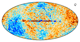
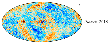
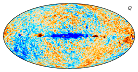
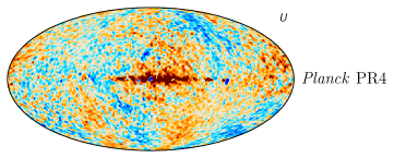
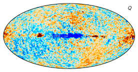
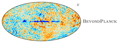
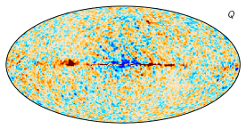
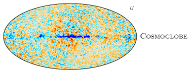
Figure 46: Difference maps between the Planck 30 GHz and WMAP K-band maps. The columns are (1) Planck 2018 v. WMAP9, (2) Planck PR4 v. WMAP9, (3) BeyondPlanck v. WMAP9, and (4) Cosmoglobe Planck 30 GHz and WMAP K-band both produced in this paper. All maps have been smoothed to a common resolution of $2^{\circ}$ FWHM, and the K-band map has been scaled by $0.495$ to account for different central frequencies, assuming a synchrotron spectral index $\beta_{\mathrm{s}}=-3.1$.

Over the last half century, a long series of technological breakthroughs have revolutionized our understanding of both cosmology and astrophysics through increasingly detailed measurements of the radio, microwave and submillimeter sky. Typically, these developments have taken place within individual experiments, each constructing novel equipment and techniques to better measure and constrain new physics while mitigating the relevant systematic effects. Each new generation of experiments has moved the frontier in terms of sensitivity, angular resolution, frequency coverage, and systematics control. This steady improvement in technological capability comes at a non-negligible cost. A typical budget for an astrophysics satellite mission ranges between 100 and 1000 million euros or dollars, and a few next-generation ground-based experiments have budgets in the hundreds of million dollar range. To make new breakthroughs in the future, we cannot afford to perform science without fully utilizing the data from experiments that have come before. Given that all experiments fundamentally observe the same sky, it is therefore essential for the field as a whole to optimally reuse all already existing state-of-the-art measurements whenever designing, fielding, and analyzing a new experiment.

This insight is the defining goal of the Cosmoglobe project; namely to integrate the world’s best data from radio to submillimeter wavelengths through global analysis. In this sentence, the word “global” carries three different meanings. First, as demonstrated by the Planck experience, it is of critical importance to analyze all aspects of a given experiment globally – instrument calibration, component separation, and cosmological interpretation – in order to understand and mitigate all relevant systematic effects. Otherwise, degeneracies between the calibration and sky model will invariably dominate the final error budget. Secondly, as demonstrated by both Planck and WMAP, virtually all experiments have some blind spots to which they are uniquely insensitive, whether it is due to frequency range, angular resolution, scanning strategy, or raw sensitivity. It is therefore always, at least in principle, advantageous to analyze multiple experiments jointly, in order to use the strengths of one experiment to break the degeneracy of another; multi-experiment analysis is thus the second aspect of global analysis. Thirdly, in order for this ambitious program to succeed, it is essential that large fractions of the community work together, and expertise from different collaborations, groups, and countries are optimally combined. International collaboration is thus the third aspect of global analysis.

This massive program would not be organizationally feasible without decades of investments in instrumentation and algorithm development by the entire field. The current Cosmoglobe implementation relies heavily on work done within the Planck collaboration, both in terms of developing the general understanding of both integrated and Bayesian parametric analysis (e.g., Planck Collaboration X 2016; Planck Collaboration II 2020; Planck Collaboration LVII 2020), as well as the specific code implementation (Commander; Eriksen et al. 2004, 2008). After the conclusion of the official Planck collaboration, this work was continued within the BeyondPlanck collaboration (BeyondPlanck 2023), which culminated in the Commander3 code (Galloway et al. 2023a), which for the first time allowed true integrated end-to-end Bayesian analysis of a major CMB experiment, namely Planck LFI. This framework provides a mature computational foundation for the Cosmoglobe analysis, which aims to apply the same process to all available state-of-the-art datasets.

The current paper represents the first step in this long process. Specifically, we have analyzed the WMAP measurements from raw time-ordered data to final CMB power spectra within one single computer code, which is a notable milestone by itself. However, this analysis accounts in fact for both WMAP and Planck LFI time-ordered data at the same time, marking an even larger milestone. It demonstrates that joint multi-experiment analysis is indeed both computationally and practically feasible. Furthermore, while the new (signal-dominated) temperature sky maps appear to be consistent with the previous state-of-the-art WMAP9 products, the new Cosmoglobe polarization maps appear to be of higher quality than the WMAP9 maps. This provides a strong testament to the original Cosmoglobe idea; better results are obtained when exploiting synergies between complementary experiments. Even moreso, we believe that this analysis demonstrates that it is in fact easier to analyze multiple experiments together because of fewer degeneracies.

Going into greater detail, we find that our gain model agrees with the WMAP9 estimates to within 1 %, despite the fact that the two approaches use very different calibration methods. This is a testament to the performance of both. In addition, our parametric noise model results in knee frequencies that are mostly consistent with the first-year WMAP values, while still tracking temporal variations on shorter timescales than those considered by the WMAP team. The transmission imbalance parameters are statistically consistent within the WMAP9 error budget, although the two methods disagree on the magnitude of the uncertainty for individual radiometers. Finally, we are able to track the goodness of fit per scan for each individual radiometer, and find that the raw $\chi^{2}$ is within 0.3 % of $n_{\mathrm{TOD}}$ throughout the entire mission.

Turning to the map domain, we note that our temperature maps are consistent with WMAP9 to about $2.5\thinspace\mathrm{\mu K}$ on large angular scales, and the remaining differences are most likely due to the different baseline and gain modeling. In polarization, we see differences of up to $\sim 10\thinspace\mathrm{\mu K}$. A large fraction of this is due to the poorly measured transmission imbalance modes identified by the WMAP team; however, we have also shown that the bilinear template marginalization method used in WMAP9 is unable to account for the full observed differences. This is of course not unexpected, given that the impact of transmission imbalance is a nonlinear effect that couples to a wide range of instrumental parameters, and two linearly dependent templates cannot account for the full posterior volume of these parameters. In contrast, by virtue of tracing all these nonlinear couplings through an explicit data model, an MCMC sampler is able to model these correlated modes naturally. As a result, we find that the large-scale residuals are visually present in internal WMAP9 half-difference DA maps, but not in the corresponding Cosmoglobe maps. Correspondingly, we find that the WMAP9 and Cosmoglobe temperature power spectra agree very well, while the $E$-mode and $B$-mode power spectra from Cosmoglobe are better behaved for nearly every multipole.

This work provides a natural resolution to the long-standing discrepancy between the polarized WMAP K-band and Planck LFI 30 GHz observations first reported by Planck Collaboration X (2016). These two channels are sufficiently close in frequency that any uncertainty in the synchrotron SED should be subdominant to instrumental noise. However, when differencing these two maps (after scaling one by the synchrotron SED), large-scale residuals correlated with the scanning strategy appeared. The Planck LFI team worked hard to improve their data processing through the Planck 2018 and PR4 release, gradually reducing systematic errors in their products. This process continued into the BeyondPlanck epoch, but even after that obvious residuals remained (Gjerløw et al. 2023). It is only now, when both LFI and WMAP are processed from scratch, that the two datasets agree to a level compatible with instrumental noise. This progress is illustrated in Fig. 46, which shows the K–30 difference maps for Planck 2018, Planck PR4, BeyondPlanck, and Cosmoglobe. In all but the last case, the Planck maps are differenced with the WMAP9 K-band map.

In turn, the successful resolution of these long-standing problems have important and direct implications for a wide range of polarization-based applications. One example of this is estimation of the synchrotron spectral index, which is addressed in a separate paper by Fuskeland et al. (2023); it is only with these new data products that it is possible to derive physically meaningful estimates of $\beta_{\mathrm{s}}$ with combined LFI and WMAP measurements on all angular scales. Correspondingly, this is the first time LFI and WMAP constraining power have been successfully combined into a single polarized synchrotron amplitude map, and the Cosmoglobe version of this map therefore represents both the most sensitive and systematically cleanest full-sky tracer of polarized emission available today. We recommend that this map should be the preferred synchrotron template in the foreseeable future, for instance when simulating the radio sky with PySM (Thorne et al. 2017) or forecasting the performance of next-generation experiments (e.g., LiteBIRD Collaboration et al. 2022; Aurlien et al. 2022). In general, we believe that these maps redefine the state-of-the-art in terms of WMAP data quality.

In terms of CMB intensity science, there are also a few interesting observations worth pointing out. First, we find a CMB Solar dipole amplitude of $3366.2\pm 1.4\thinspace\mathrm{\mu K}$, which is $2.5\thinspace\sigma$ higher than the closely related BeyondPlanck analysis (Colombo et al. 2023). This is very close to the final Planck PR4 value of $3366.6\pm 2.6\thinspace\mu$K, and the combination of WMAP and LFI now agree very well with the independent HFI measurements. Second, we find a lower quadrupole amplitude than latest Planck results of $\sigma_{2}=131\pm 69\thinspace\mathrm{\mu K^{2}}$. Although statistically consistent with the $\Lambda$CDM prediction at the 11 % level, it is still interesting to note that this is lower than all previous estimates, except for the first-year WMAP release. Third, it is also intriguing to note that the peak of the octopole alignment statistic posterior peaks at unity, which, if true, could potentially hint towards physics beyond the $\Lambda$CDM model, for instance in the form of nontrivial topology. An important goal for future work is to decrease this – and all other – uncertainty by adding additional data and improved data models. In particular the integration of Planck HFI measurements is a high priority for future work.

We believe that this first Cosmoglobe data release successfully demonstrates the advantages of global data analysis, and we hope and anticipate that it is only the first among many, each adding support for one or more new experiments. We invite all interested parties to join this effort, whether it is by providing access to experimental data, novel algorithmic ideas, or just sheer work force; for further details on how to contribute, we refer the interested reader to the Cosmoglobe webpage.

Appendix A Survey of instrumental parameters

In this Appendix, we provide for reference purposes a complete survey of the posterior mean estimates for all time-dependent instrumental parameters. In each figure, columns correspond to individual diodes, while rows correspond to DA. Figure A shows the zeroth order baseline (plotted as the difference between the full time-variable baseline and its own time average), while Fig. 48 shows the corresponding baseline slopes. Figure 49 shows the full time-dependent gain, and Fig. 50 shows the fractional gain difference between Cosmoglobe and WMAP in units of percent. Figures 51–53 shows the noise model parameters, $\sigma_{0}$, $f_{\rm knee}$, and $\alpha$, respectively. Finally, Fig. 54 shows the TOD-level reduced normalized $\chi^{2}$ in units of standard deviation. Black lines show Cosmoglobe results, while solid red lines show (where available) official WMAP results derived by linear regression between the raw and calibrated WMAP TODs. Orange and red dotted lines show WMAP first-year in-flight and GSFC laboratory measurements, respectively. For further discussion regarding these plots, see Sect. 4.

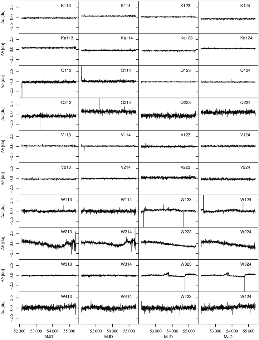
Figure 47: Difference in zero-level baseline between Cosmoglobe and WMAP9, $b_{0}^{\mathrm{CG}}-b_{0}^{\mathit{WMAP}}$.

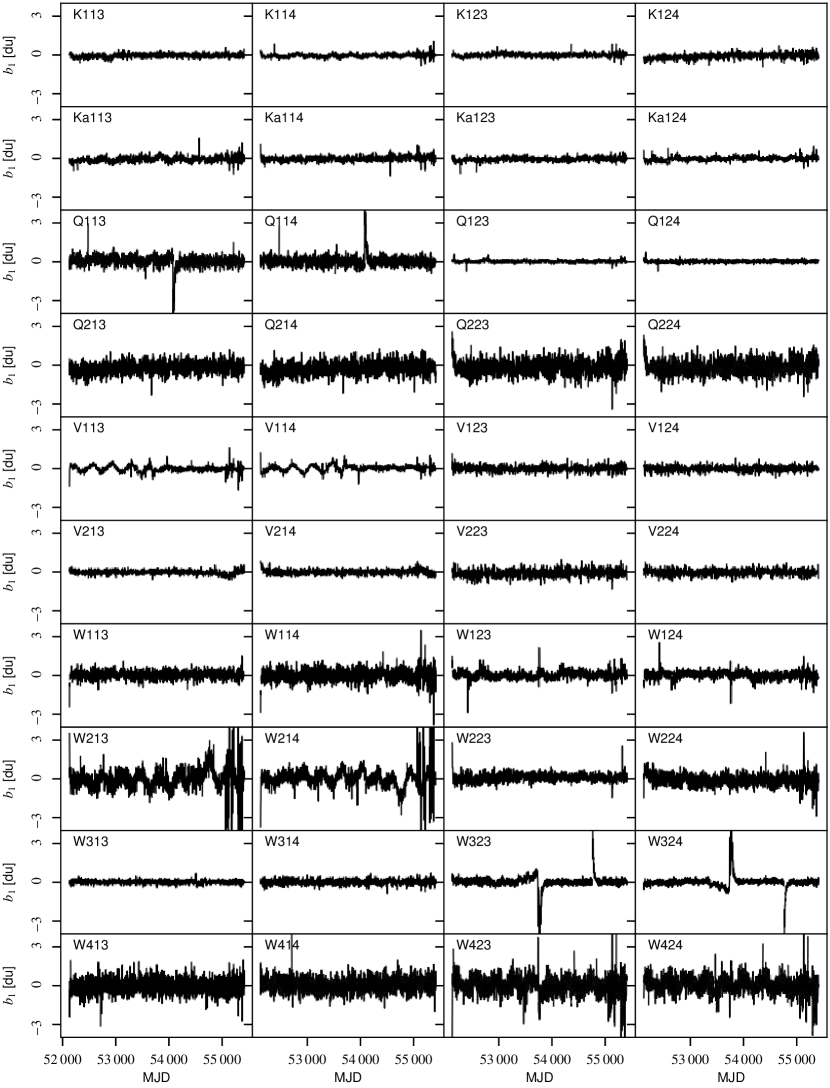
Figure 48: Cosmoglobe first-order baseline correction (i.e., slope) for each diode.

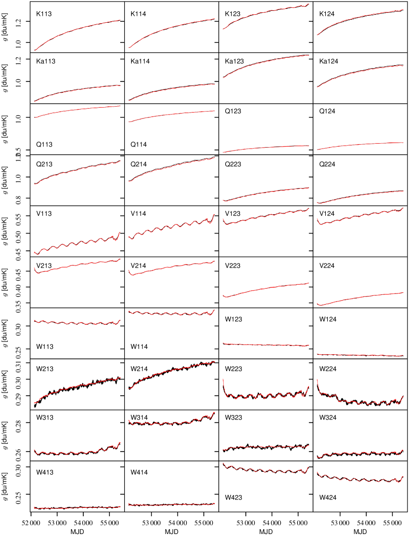
Figure 49: Time-variable gain model for each diode for Cosmoglobe (black) and WMAP9 (red).

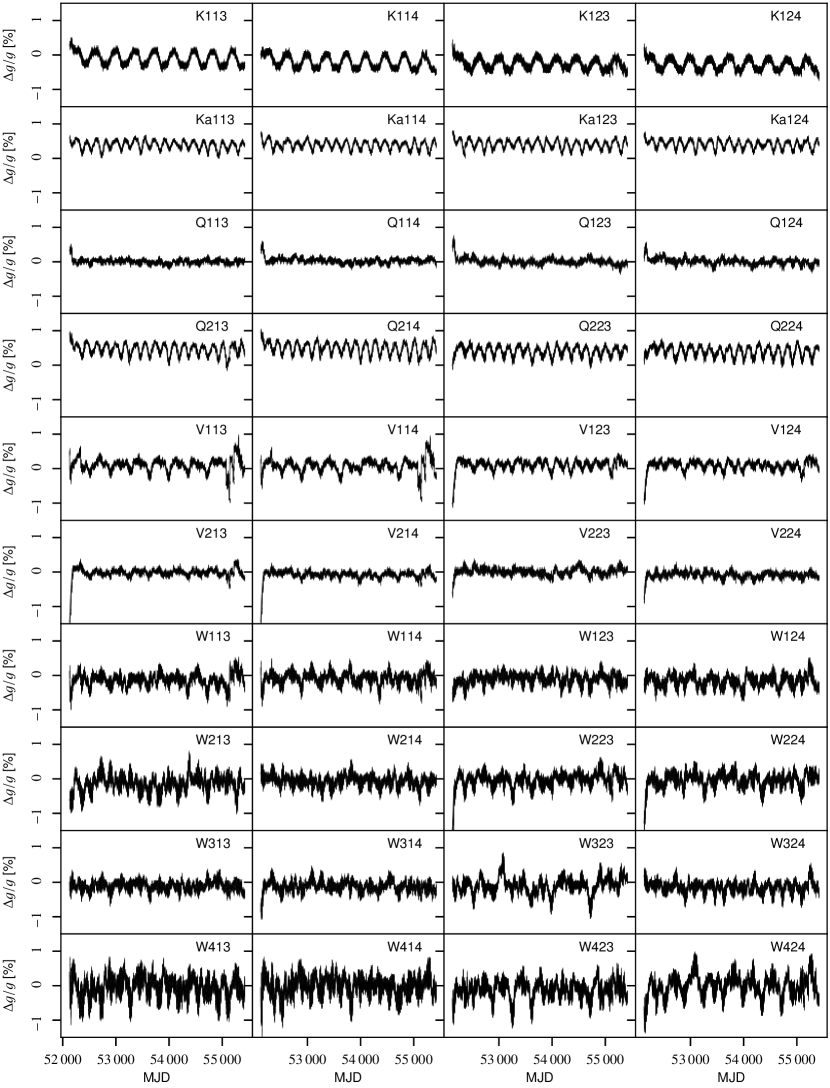
Figure 50: Relative gain difference between Cosmoglobe and WMAP9, $(g^{\mathrm{CG}}-g^{\mathit{WMAP}})/g^{\mathit{WMAP}}$.

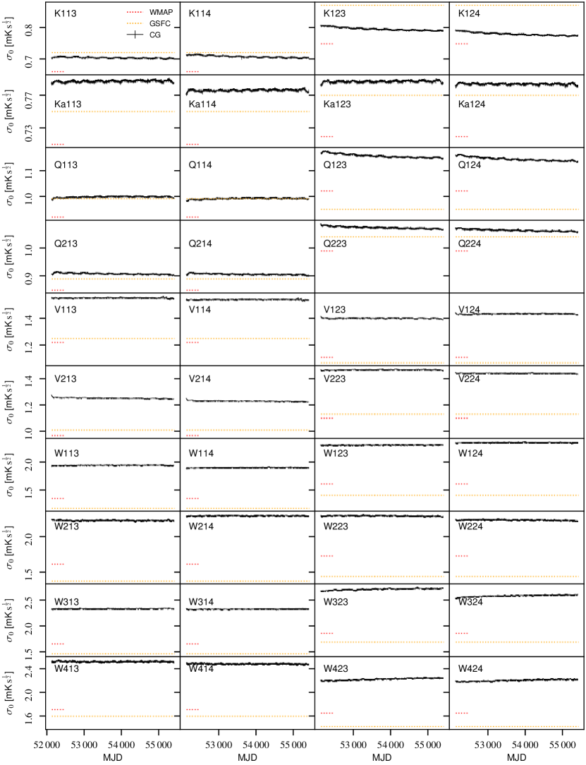
Figure 51: White noise rms per TOD sample, $\sigma_{0}$. Black lines show Cosmoglobe estimates, while dotted red and orange lines show WMAP first-year in-flight and GSFC laboratory measurements.

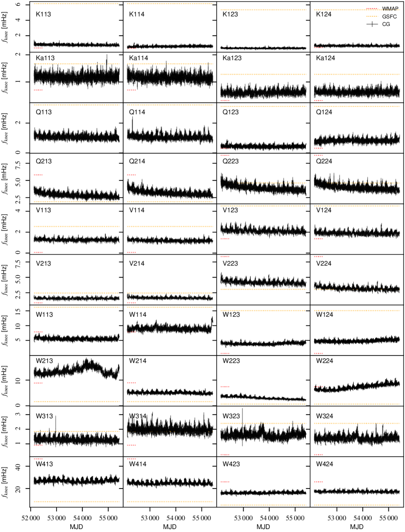
Figure 52: Correlated noise knee frequency, $f_{\mathrm{knee}}$, for each diode. Black lines show Cosmoglobe estimates while dotted red and orange lines show WMAP first-year in-flight and GSFC laboratory measurements.

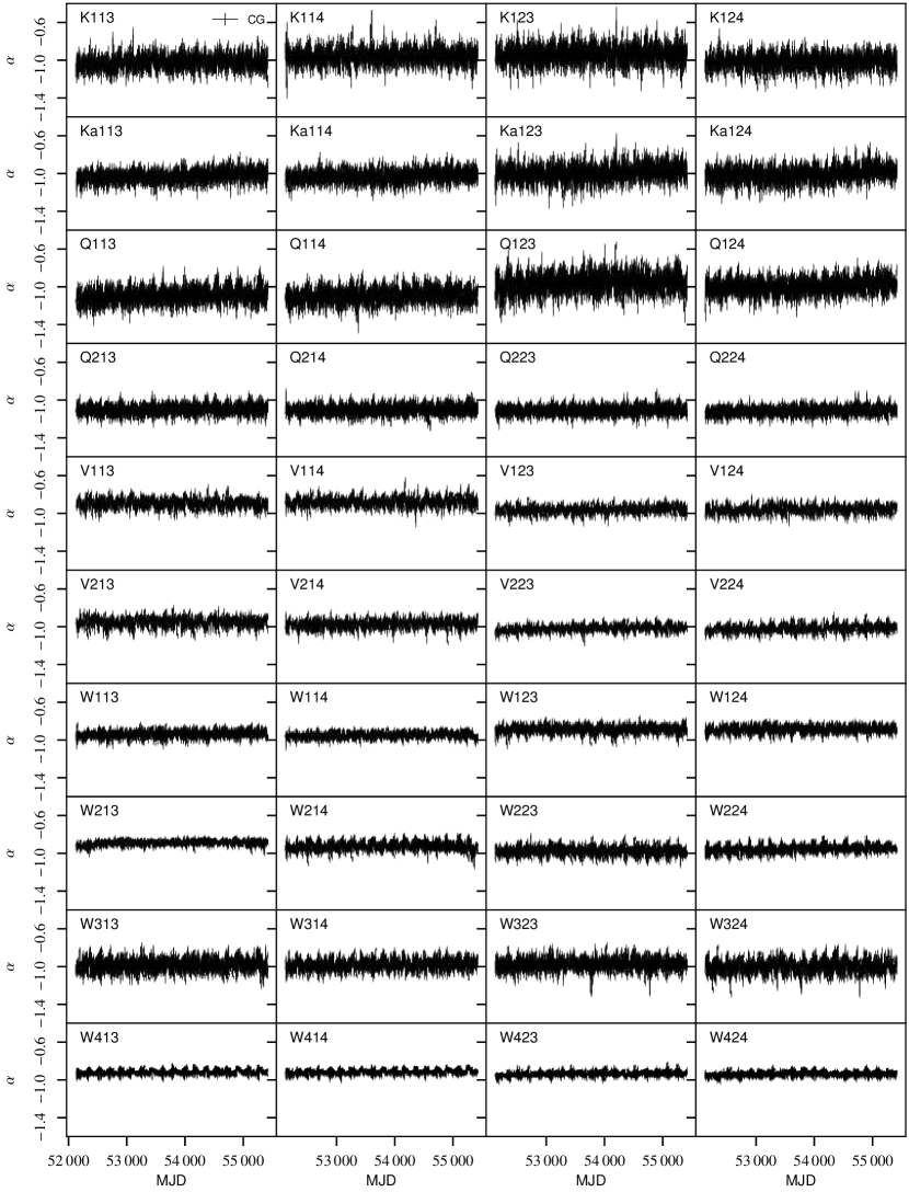
Figure 53: Correlated noise slope, $\alpha$, for each diode. Black lines show Cosmoglobe estimates, while dotted orange and red lines show WMAP first-year in-flight and GSFC laboratory measurements.

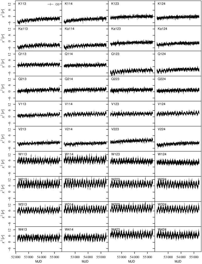
Figure 54: TOD-level reduced normalized $\chi^{2}$ as defined by Eq. (17).

Appendix B WMAP frequency map survey

In this appendix, we provide a frequency map survey for all ten DAs. Figure B shows the full DA polarization maps as derived both by Cosmoglobe and WMAP9, as well as their differences. Figures 56 and 57 shows Cosmoglobe white noise and posterior rms for each DA and Stokes parameter, as well as the cross-correlation between Stokes $Q$ and $U$. Figure 58 shows differences between two Gibbs samples, Figs. 59 and 60 show the TOD-level correlated noise and residual, respectively, both obtained by projecting the timestreams into sky maps. Finally, Fig. 61 shows the map-level residual, obtained by subtracting the astrophysical sky model from the corresponding DA map.

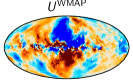
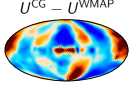
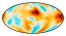
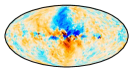
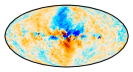
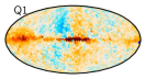
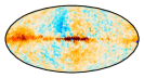
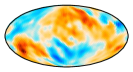
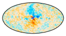
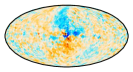
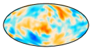
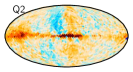
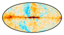
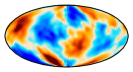
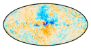
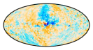
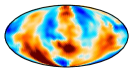
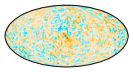
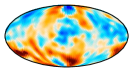
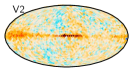
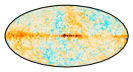
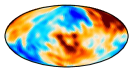
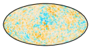
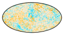
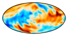
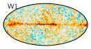
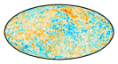
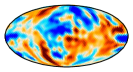
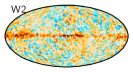
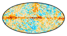
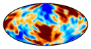
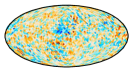
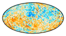
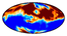
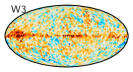
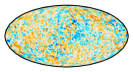
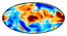
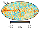
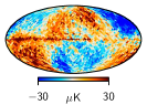
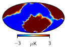
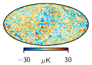
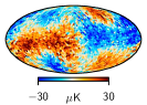
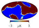
Figure 55: Comparison of Cosmoglobe and WMAP9 polarization DA maps. Left and right sections show Stokes $Q$ and $U$, respectively, while rows show DAs. Within each section, the left and middle columns show the Cosmoglobe and WMAP9 maps, while the right column shows their difference. All full-signal maps are shown at a HEALPix resolution of $N_{\mathrm{side}}=16$, and the difference maps have additionally been smoothed with a $10^{\circ}$ FWHM beam.

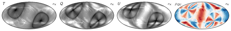
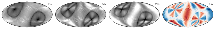
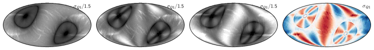
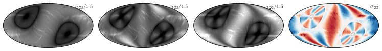
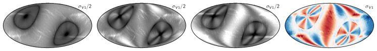
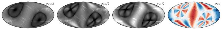
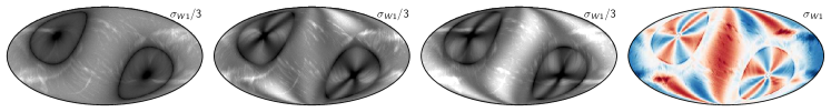
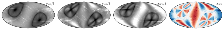
Figure 56: Cosmoglobe white noise rms per pixel, $\sigma_{p}$, for each DA and Stokes parameters. The rightmost column shows the cross-correlation between Stokes $Q$ and $U$ due to the WMAP scanning strategy.

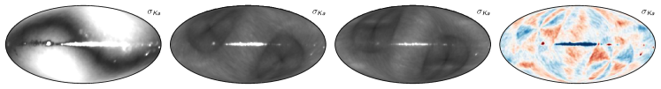
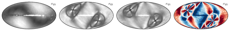
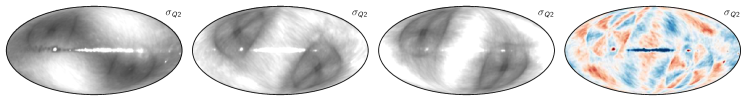
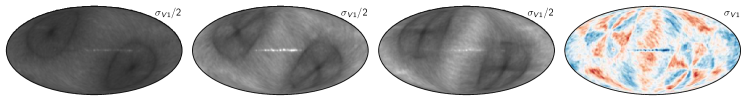
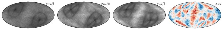
Figure 57: Cosmoglobe posterior standard deviation for each DA and Stokes parameter, evaluated at an angular resolution of $2^{\circ}$ FWHM. The rightmost column shows the correlation coefficient between Stokes $Q$ and $U$.

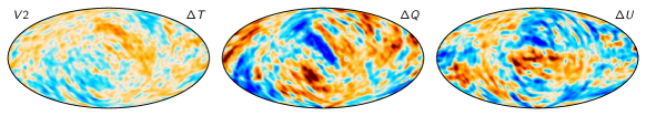
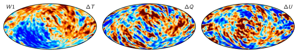
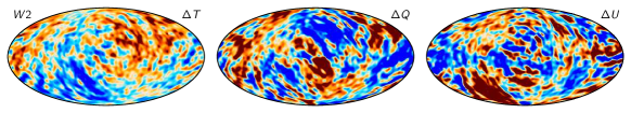
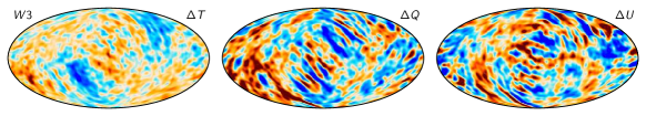
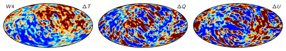
Figure 58: Differences between two Cosmoglobe frequency map samples, smoothed with a $5^{\circ}$ FWHM Gaussian beam.

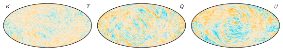
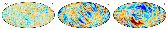
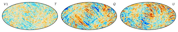
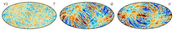
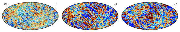
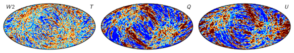
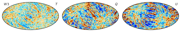
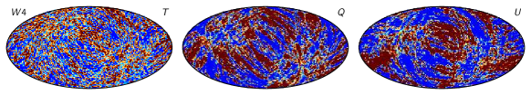
Figure 59: Binned correlated noise timestreams for each DA, smoothed with a $2^{\circ}$ FWHM Gaussian beam.

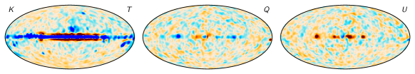
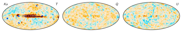
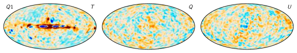
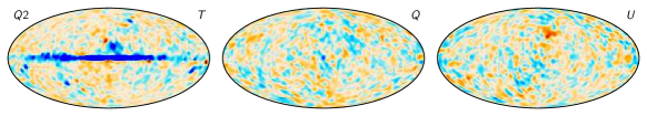
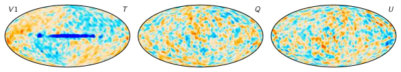
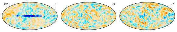
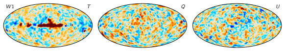
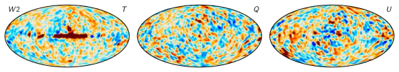
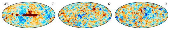
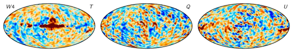
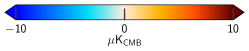
Figure 60: Binned TOD-level residuals for each DA, smoothed with a $5^{\circ}$ FWHM Gaussian beam.

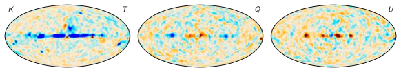
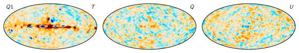
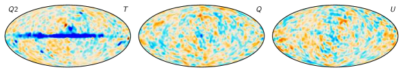
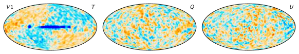
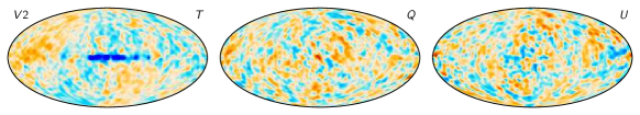
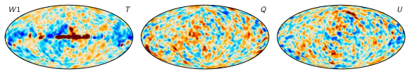
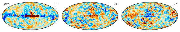
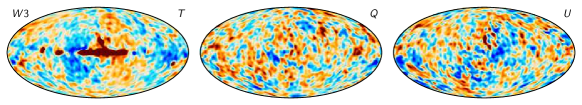
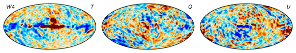
Figure 61: Map-level residuals for each DA, smoothed by $5^{\circ}$.