Interpretable ODE-style Generative Diffusion Model via Force Field Construction

Abstract

For a considerable time, researchers have focused on developing a method that establishes a deep connection between the generative diffusion model and mathematical physics. Despite previous efforts, progress has been limited to the pursuit of a single specialized method. In order to advance the interpretability of diffusion models and explore new research directions, it is essential to establish a unified ODE-style generative diffusion model. Such a model should draw inspiration from physical models and possess a clear geometric meaning. This paper aims to identify various physical models that are suitable for constructing ODE-style generative diffusion models accurately from a mathematical perspective. We then summarize these models into a unified method. Additionally, we perform a case study where we use the theoretical model identified by our method to develop a range of new diffusion model methods, and conduct experiments. Our experiments on CIFAR-10 demonstrate the effectiveness of our approach. We have constructed a computational framework that attains highly proficient results with regards to image generation speed, alongside an additional model that demonstrates exceptional performance in both Inception score and FID score. These results underscore the significance of our method in advancing the field of diffusion models.

1 Introduction

Deep generative models have found successful applications in several fields such as computer vision [2], density estimation [19], natural language processing [3], and semi-supervised learning [15]. They also provide a promising paradigm for unsupervised learning. However, despite their popularity, current deep generative models face several limitations. These limitations include training instability of GANs [2, 7, 12], sample quality issues of VAEs [23], normalized flow [16, 21], and slow sampling speed of diffusion [10, 26, 32, 11] and score-based models [27]. Recently, Poisson flow generation model (PFGM) [31] proposed an ODE-like generative-diffusion model inspired by Coulomb force, which has a clear geometric meaning. Although this approach is intuitive in physics, Coulomb force is not the only option for model building, and it seems possible to construct other forms of force using the same physical painting. Furthermore, while the model’s physics-based foundation is strong, there is a lack of mathematical proof that it can learn the process of moving along the field line from an arbitrary point in the distance to a certain Coulomb force source data distribution. As such, it is imperative for researchers to investigate alternative modes of energy to foster model development, while concurrently providing a rigorous mathematical validation of the learning mechanism inherent to the ODE-based generative-diffusion model of PFGM.

To address the issue of determining the appropriate force field for constructing an ODE-style generative diffusion model, we propose a review of the fundamental task of the diffusion model. This task involves transforming samples from a simple distribution to samples from a target distribution by constructing a suitable transformation. Theoretically, constructing an ODE-style diffusion model [27] is equivalent to solving a relaxed and almost unconstrained indeterminate equation.

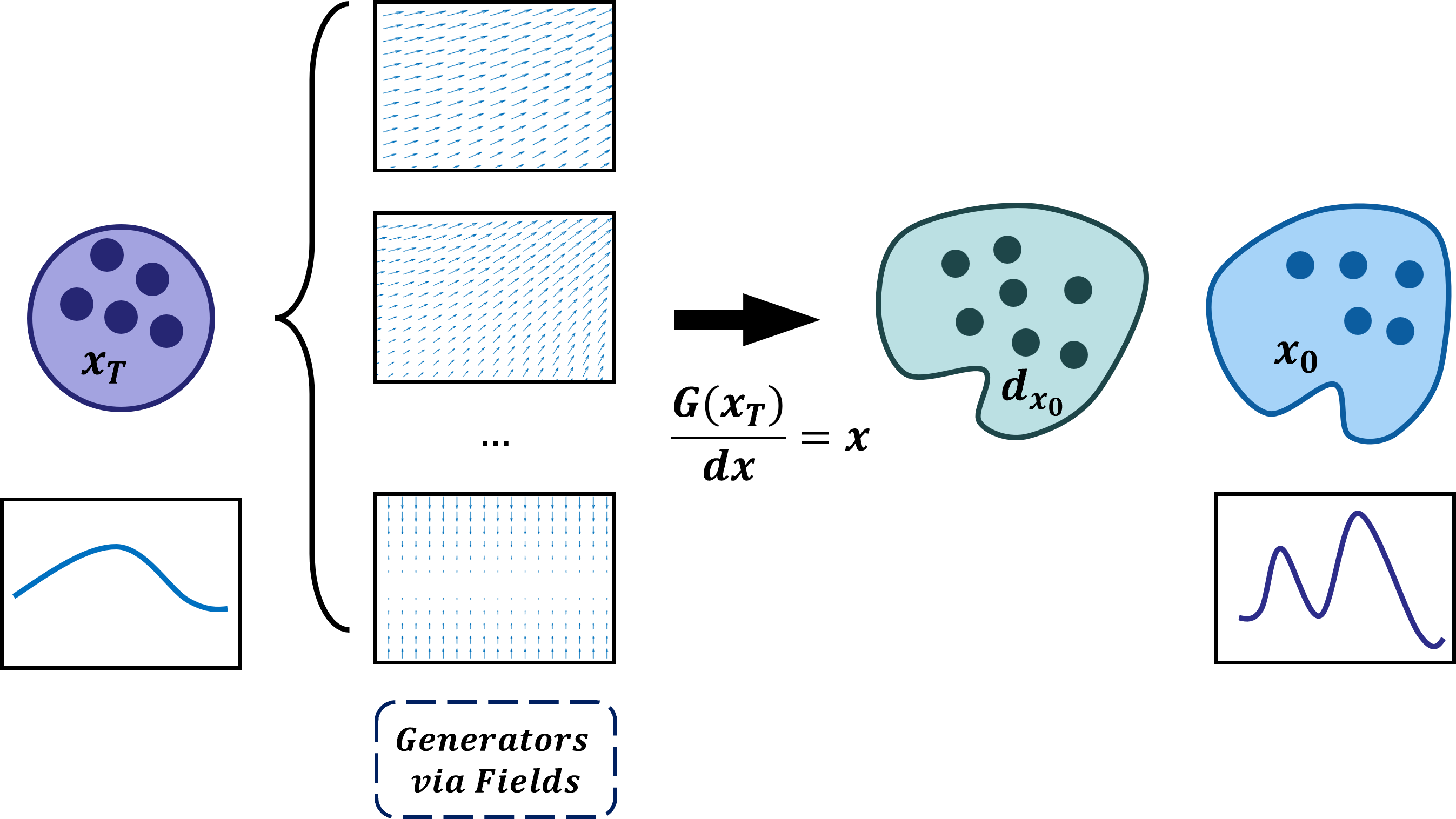
Figure 1: The process of generative model based on force field.

Previous research has proposed specialized solutions for generative diffusion models, such as PFGM. This model utilizes Coulomb’s law to construct a potential function that is inversely proportional to the $Nth$ power, forming the basis of the kinetic model. Using the field of potential functions, a flow model is defined where the probability distribution evolves based on the gradient flow $\partial p_{t}(\mathbf{x})/\partial t=-\nabla\cdot\left(p_{t}(\mathbf{x})\mathbf{E}(\mathbf{x})\right)$. It is worth noting that gradient flow is a special case of the Fock-Planck equation [24]. The solution proposed by PFGM is an indeterminate equation with $d+1$ unknowns and one equation, indicating that there are potentially infinite solutions in theory. To derive a practical solution, additional assumptions are necessary.

In this paper, we provide a mathematical proof that the physical model we constructed is capable of learning the target data distribution. Additionally, we present a unified method for identifying the appropriate force field for the generative diffusion model and summarize the construction process of this model in detail. A series of technical contributions we made are as follows. In practical applications, data distribution migration is achieved through solving a set of coupled forward and backward ordinary differential equations induced by a force field (refer to Figure 2).

Starting from geometric intuition, we construct a specific vector field to ensure that the result satisfies the initial value distribution conditions, and then solve the differential equation to ensure the final value distribution conditions, and obtain a Green’s function that satisfies both the initial value and the final value conditions. In particular, this method allows us to use arbitrary simple distributions as prior distributions, freeing us from previous reliance on Gaussian distributions to construct diffusion models. Finally, in experiments, we find two force field construction methods that perform well in terms of speed and image generation quality through this method.

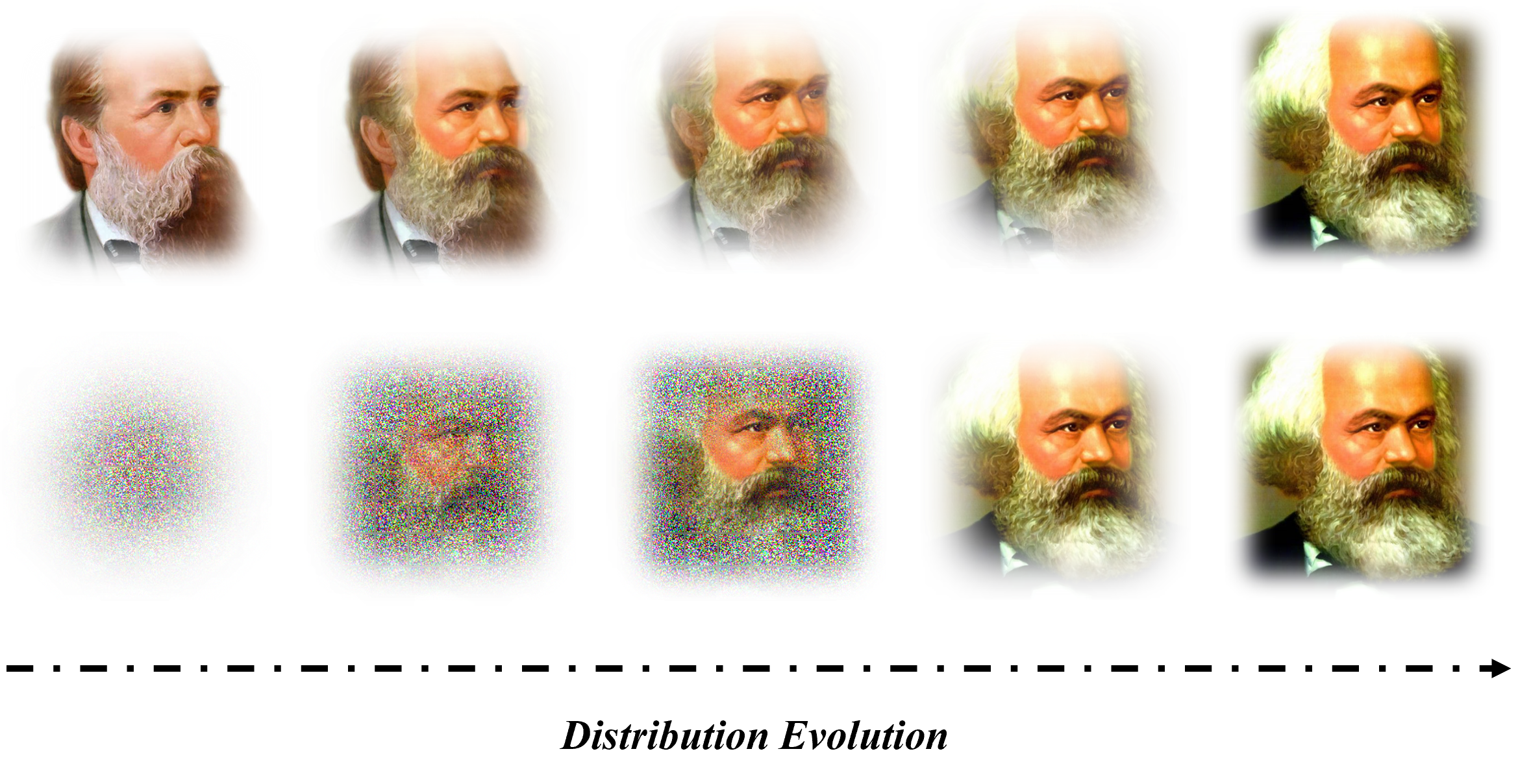
Figure 2: The evolutions of a distribution by the field.

2 Related Works

Normalizing Flow. Taking image generation as an example, the idea of Normalizing Flow [16, 21] is to find an invertible function $f$, which can convert the distribution of $X$ to a known simple distribution (such as Gaussian distribution) for an image set $X$. Then generating graphics becomes very simple, as long as a point is sampled from a known simple distribution, and then through the inverse function of $f$, the picture can be generated. The Continuous Normalizing Flows (CNFs) [18] propose the concept of Flow Matching (FM), a simulation-free method for training CNFs based on regression vector fields with fixed conditional probability paths. Compared with Variational Autoencoder (VAE), the Normalizing Flow method [5] has achieved better performance in various image tasks.

Score-based Generative Models. Score-based generative model [27] learns a kind of score functions, that is, gradients of log probability density functions, on large-scale noise-perturbed data distributions, and uses Langevin to sample samples that conform to the training set. In denoising diffusion probabilistic models (DDPM) [10, 26, 32, 11], the diffusion process is divided into fixed T steps. In fact, the real data transformation process should have no deliberate steps, and they can be understood as a continuous transformation process in time, described by Stochastic Differential Equation (SDE) [27]. Therefore, the advantage of this method is that it can get the sampling effect of GAN level without confrontation learning. At the same time, it has uniquely identifiable representation learning [1] at the level of interpretability.

Poisson Flow Generation Model. Poisson flow generation model [31] is an ODE-style diffusion model inspired by ”Coulomb’s Law”, which breaks through the dependence of many previous diffusion models on Gaussian assumptions, and is a new framework for constructing ODE-style diffusion models based on field theory. Therefore, our subsequent work will focus on mathematically proving how to finally learn the data distribution and the expansion of various field forms, and on the premise of finding out what kind of force field is suitable for building an ODE-style generative diffusion model, we can obtain a brand-new force field diffusion model that adapts to different requirements is developed.

3 Background Knowledge

Transport Equation. The transport equations can be expressed by flux integrals applicable to any finite area or by divergence operators applicable to a certain point. In this paper, Fourier’s heat conduction equation will be used

$$\frac{\partial}{\partial t}F_{t}(\boldsymbol{x}_{t})=D_{t}\nabla_{\boldsymbol{x}_{t}}^{2}F_{t}(\boldsymbol{x}_{t})$$ (1)

where $\boldsymbol{D}_{t}(\boldsymbol{x}_{t})$ is a non-negative scalar function used to construct a loss function solution.

Mode Collapse. The Poisson flow generative model proposes a concept of mode collapse [31]. This collapse comes from the force field offset generated by the isotropic solution, so it is necessary to add an additional dimension when constructing the force field model. In the experimental part of this paper, the mode collapse of the multi-sample straight line case will also be discussed.

Generative Modeling via Force Fields. Generative modeling can enable the transformation of a base distribution into a data distribution through trajectories defined by li force fields. Distribution-based samplers allow for adaptive sampling, accurate likelihood assessment, and modeling of continuous-time dynamics. For sampling, the learned reversible mappings can be directly integrated.

Dirac Delta Function. The modeling of particles and point charges relies on the concept of limits, whereby the volume is made infinitely large. However, this results in an infinite density of particles or charge density of point charges, which can be resolved by integrating the density in space to obtain a finite mass or charge. To describe such a density distribution, the Dirac delta function is employed. This scenario aligns with the initial value conditional constraints of the generator, which produces the data points in the model, and serves as a necessary demonstration of the solvability of the dynamical differential equation.

4 Method

4.1 Construct the Force Field Equation

Preparatory Work. Consider the system of first-order ordinary differential equations $\frac{d\boldsymbol{x}_{t}}{dt}=\boldsymbol{F}_{t}(\boldsymbol{x}_{t})$ of $\boldsymbol{x}_{t}\in\mathbb{R}^{d},t\in(0,T)$. It describes a reversible transformation from $\boldsymbol{x}_{0}$ to $\boldsymbol{x}_{T}$. If $\boldsymbol{x}_{0}$ is a random variable, then $\boldsymbol{x}_{t}$ in the whole process is also a random variable. This distribution law can be described by the following equation

$$\frac{\partial}{\partial t}d_{t}(\boldsymbol{x}_{t})=-\nabla_{\boldsymbol{x}_{t}}\cdot\Big{(}\boldsymbol{F}_{t}(\boldsymbol{x}_{t})d_{t}(\boldsymbol{x}_{t})\Big{)}$$ (2)

The formulation of this equation is motivated by the transport equation in physics that characterizes the scenario where energy can only propagate through a continuous flux, bearing a striking resemblance to the diffusion model. The objective of the model is to develop a transformation that converts samples originating from a basic distribution into samples that conform to a desired target distribution. Equation (2) enables one to identify the appropriate $F_{t}(\boldsymbol{x}_{t})$ for a given $d_{t}(\boldsymbol{x}_{t})$ in principle.

Solving ODE Equations. First, by transposing Equation (2) to get $\left({\partial}/{\partial t},\nabla_{\boldsymbol{x}_{t}}\right)\cdot(d_{t}(\boldsymbol{x}_{t}),\boldsymbol{F}_{t}(\boldsymbol{x}_{t})d_{t}(\boldsymbol{x}_{t}))=0$, $\left({\partial}/{\partial t},\nabla_{\boldsymbol{x}_{t}}\right)$ can be regarded as a $d+1$ dimensional gradient, $\big{(}p_{t}(\boldsymbol{x}_{t}),\boldsymbol{F}_{t}(\boldsymbol{x}_{t})d_{t}(\boldsymbol{x}_{t})\big{)}$ can just form a $d+1$ vector , so Equation (2) can be written as a simple divergence equation $\nabla_{(t,\,\boldsymbol{x}_{t})}\cdot\boldsymbol{v}(t,\boldsymbol{x}_{t})=0$. In this way, it is not difficult for us to combine the general form of ODE to deduce the equation

$$\frac{d\boldsymbol{x}_{t}}{dt}=\boldsymbol{F}_{t}(\boldsymbol{x}_{t})=\frac{\boldsymbol{v}_{i(i>1)}(t,\boldsymbol{x}_{t})}{\boldsymbol{v}_{1}(t,\boldsymbol{x}_{t})}$$ (3)

Since our purpose is to derive the generated target sample distribution, there will be an initial value constraint such that $\boldsymbol{v}_{1}=d_{0}(\boldsymbol{x}_{0})$. This constraint unifies the probability and distribution of the initial distribution. Equation (3) describes the trajectory of data points moving along the field lines. For such a conditional differential equation, by introducing a function $\boldsymbol{H}(x)$ to assist the solution

$$\left\{\begin{aligned} &\nabla_{(t,\,\boldsymbol{x}_{t})}\cdot\boldsymbol{H}(t,0;\boldsymbol{x}_{t},\boldsymbol{x}_{0})=0\\ &\boldsymbol{H}_{1}(0,0;\boldsymbol{x}_{t},\boldsymbol{x}_{0})=\delta(\boldsymbol{x}_{t}-\boldsymbol{x}_{0})\\ &\boldsymbol{H}_{1}(t,0;\boldsymbol{x}_{t},\boldsymbol{x}_{0})d\boldsymbol{x}_{t}=1\end{aligned}\right.$$ (4)

From this a feasible solution can be deduced: $\boldsymbol{v}(t,\boldsymbol{x}_{t})=\mathbb{E}_{(\boldsymbol{x}_{0})}[\boldsymbol{H}(t,0;\boldsymbol{x}_{t},\boldsymbol{x}_{0})]$. Among them, $\boldsymbol{H}(t,0;\boldsymbol{x}_{t},\boldsymbol{x}_{0})$ is another way of expressing the conditional probability in the score-based model [27]. In particular, the defined $\boldsymbol{H}(t,0;\boldsymbol{x}_{t},\boldsymbol{x}_{0})$ still has the properties similar to the divergence function in mathematics, and it itself can be equivalent to the force field produced by the point source. Therefore, in the subsequent construction of the force field model, we use the properties of the $H(x)$ function to superimpose different force field trajectories to achieve different model effects, and find the model we need among them.

4.2 Solutions for Special Case

Now, we proceed to solve specific results within the aforementioned framework. As previously mentioned, the aforementioned equations represent a type of indeterminate equations, which theoretically possess infinitely many solutions. However, in order to obtain a more clear solution, we need to introduce additional assumptions.

An isotropic assumption was put forward in the PFGM [31]. This means that ${H}(t,0;\boldsymbol{x}_{t},\boldsymbol{x}_{0})$ points to the source point $(0,\,\boldsymbol{x}_{0})$, and the modulus length only depends on $R=\sqrt{(t-0)^{2}+\|\boldsymbol{x}_{t}-\boldsymbol{x}_{0}\|^{2}}$. Accordingly, it can be assumed that

$$\boldsymbol{H}(t,0;\boldsymbol{x}_{t},\boldsymbol{x}_{0})=\varphi(R)(t,\boldsymbol{x}_{t}-\boldsymbol{x}_{0})$$ (5)

Thus, a unique solution situation is constructed. Substituting the first equation in Equation (4), it can be deduced that $0=\nabla_{(t,\,\boldsymbol{x}_{t})}[\varphi(R)(t,\boldsymbol{x}_{t}-\boldsymbol{x}_{0})]$. And then come to $\varphi(R)=A\times R^{-(d+1)}$. Finally, it is not difficult to have

$$\boldsymbol{H}(t,0;\boldsymbol{x}_{t},\boldsymbol{x}_{0})=A\frac{(t,\boldsymbol{x}_{t}-\boldsymbol{x}_{0})}{\left(t^{2}+\|\boldsymbol{x}_{t}-\boldsymbol{x}_{0}\|^{2}\right)^{(d+1)/2}}$$ (6)

Where $A$ represents a constant derived from the homogeneous solution of the differential equation for $\varphi(R)$. The existence of a solution notwithstanding, it is imperative to test whether the equation is solvable, which calls for a test based on the constraints imposed by Equation (5). A constructive integral is employed for this purpose, given by

$$\int\boldsymbol{H}_{1}d\boldsymbol{x}_{t}=A\int\frac{t}{\left(t^{2}+\|\boldsymbol{x}_{t}-\boldsymbol{x}_{0}\|^{2}\right)^{(d+1)/2}}d\boldsymbol{x}_{t}$$ (7)

Here, $t$ and $\boldsymbol{x}_{t}$ can be eliminated by substitution. Let $\boldsymbol{x}=(\boldsymbol{x}_{t}-\boldsymbol{x}_{0})/t$, then the points in the original equation take the following form

$$\boldsymbol{H}_{1}(t,0;\boldsymbol{x}_{t},\boldsymbol{x}_{0})d\boldsymbol{x}_{t}=A\int\frac{1}{\left(1+|\boldsymbol{x}|^{2}\right)^{(d+1)/2}}d\boldsymbol{x}$$ (8)

It is evident that the points result and the quantities of $\boldsymbol{x}_{t}$ and $t$ are independent. With the help of a constant conversion, the $H(x)$ function can be shown to be equal to one.

It can be observed that the particular solution bears a formal resemblance to the solution class proffered by the PFGM. Hence, we may infer that the Coulomb force’s physical dynamic structure is a distinct instance of the equation, and as such, may be extended to more general cases.

4.3 Establish Force Field Learning Mode

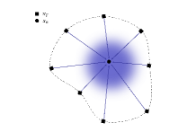
(a) One Sample Line

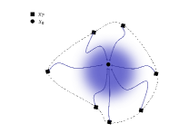
(b) Curve

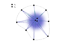
(c) Multiple Sample Line

Figure 3: A variety of different trajectories from ${x}_{T}$ to ${x}_{0}$.

Convert a trainable target. First, construct a force field function that can be used $\boldsymbol{L}_{t}(\boldsymbol{x}_{t}|\boldsymbol{x}_{0})=\boldsymbol{x}_{T}$. The aforementioned construct pertains to a cluster of trajectories, characterized by a fixed starting point $\boldsymbol{x}_{0}$ and an arbitrary end point $\boldsymbol{x}_{T}$. In this construct, the independent and dependent variables are represented by $t$ and $\boldsymbol{x}_{t}$, respectively. Notably, the starting point remains unchanged while the end point can be varied at will. Substituting ${x}_{T}$ from it to Equation (4), we can get $\boldsymbol{H}(t,0;\boldsymbol{x}_{t},\boldsymbol{x}_{0})=d_{t}(\boldsymbol{x}_{t}|\boldsymbol{x}_{0})\boldsymbol{F}_{t}(\boldsymbol{x}_{t}|\boldsymbol{x}_{0})$. Upon derivation, the subsequent objectives can be acquired

$$\mathbb{E}_{\boldsymbol{x}_{0},\boldsymbol{x}_{t}\sim d_{t}(\boldsymbol{x}_{t}|\boldsymbol{x}_{0})d_{0}(\boldsymbol{x}_{0})}\left[\left\|\boldsymbol{s}_{\boldsymbol{\theta}}(\boldsymbol{x}_{t},t)-\boldsymbol{F}_{t}(\boldsymbol{x}_{t}|\boldsymbol{x}_{0})\right\|^{2}\right]$$ (9)

Equation (9) describes the objective function of training in terms of score matching, where $\theta$ represents the training parameter. The goal is to learn a model $\boldsymbol{s}_{\boldsymbol{\theta}}(\boldsymbol{x}_{t},t)$ that approximates $\boldsymbol{F}_{t}(\boldsymbol{x}_{t}|\boldsymbol{x}_{0})$, which can be expressed in various ways, such as using $\nabla_{\boldsymbol{x}_{t}}\log p_{t}(\boldsymbol{x}_{t})$ in the probability model [10, 26, 32]. In our case, we represent it using the inspired force field method as a set of force field trajectory modes. Finally, we use network design and sampling to improve the learning of this score matching function.

Introduction of target trajectories. We define three regression processes from ${x}_{T}$ to ${x}_{0}$ through the above method: linear type, distribution type, and curve type.

$$\left\{\begin{aligned} &d_{t}(\boldsymbol{x}_{t}|\boldsymbol{x}_{0})=\frac{d_{T}\left(\frac{\boldsymbol{x}_{t}-\boldsymbol{x}_{0}}{t}+\boldsymbol{x}_{0}\right)}{t^{N}}\\ &d_{t}(\boldsymbol{x}_{t}|\boldsymbol{x}_{0})=\frac{d_{T}\left(\frac{\boldsymbol{x}_{t}-\boldsymbol{\mu}_{t}({x}_{0})}{{{\sigma}_{t}}}\right)}{{{\sigma}_{t}}^{N}}\\ &d_{t}(\boldsymbol{x}_{t}|\boldsymbol{x}_{0})=\frac{d_{T}\left(\frac{(t-1)(\boldsymbol{x}_{t}-\boldsymbol{x}_{0})}{t^{m}}\right)}{t^{Nm}}\end{aligned}\right.$$ (10)

Taking the straight line type as an example, we can perform a simple derivation. For a linear relationship, the vector form of the line can be written $\boldsymbol{x}_{t}=(\boldsymbol{x}_{T}-\boldsymbol{x}_{0})t+\boldsymbol{x}_{0}$. Then according to the differential equation established above, there will be $\nabla_{\boldsymbol{x}_{t}}\cdot\boldsymbol{F}_{t}(\boldsymbol{x}_{t}|\boldsymbol{x}_{0})=\frac{d}{t}$. Finally, the above conclusion can be drawn.

Figure 3 employs a geometric approach to illustrate the movement of single-sample data points across various trajectories under different conditions when $T=1$. Further, Figure 3(a) depicts the transformation process from a fixed sampling pattern to the original distribution in the case of a single-sample force field trajectory, where the sample points move linearly, resulting in high generation efficiency. In contrast, Figure 3(b) illustrates the curved trajectory, which can adaptively fit the information hot spots of the sample under different force fields, while mitigating the influence of singularities and achieving better model robustness. Finally, Figure 3(c) demonstrates a multi-sample straight line force field trajectory, which combines both straight line trajectories and curved trajectories to achieve good performance. As the sample size increases, the force field becomes more complex and the trajectory can be fitted to a more intricate situation. Therefore, we propose two approaches for identifying the most suitable training method: 1) utilizing a single straight line for multiple multi-sample training to fit various distributions, and 2) directly sampling multiple measurements far apart using a curved trajectory. These approaches will be discussed separately in Section 5 of the experiment, and a better solution will be determined based on the specific conditions.

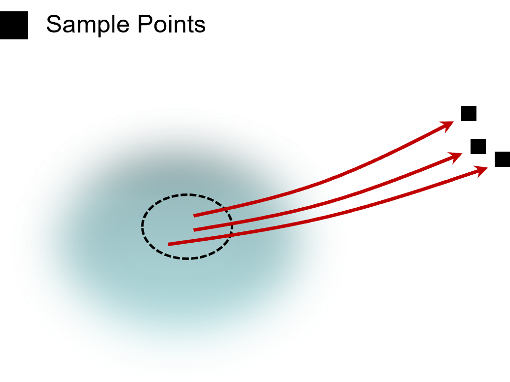
(a) Gaussian Distribution

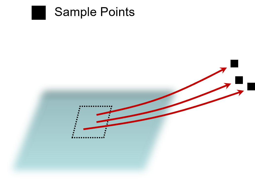
(b) One Sample Line

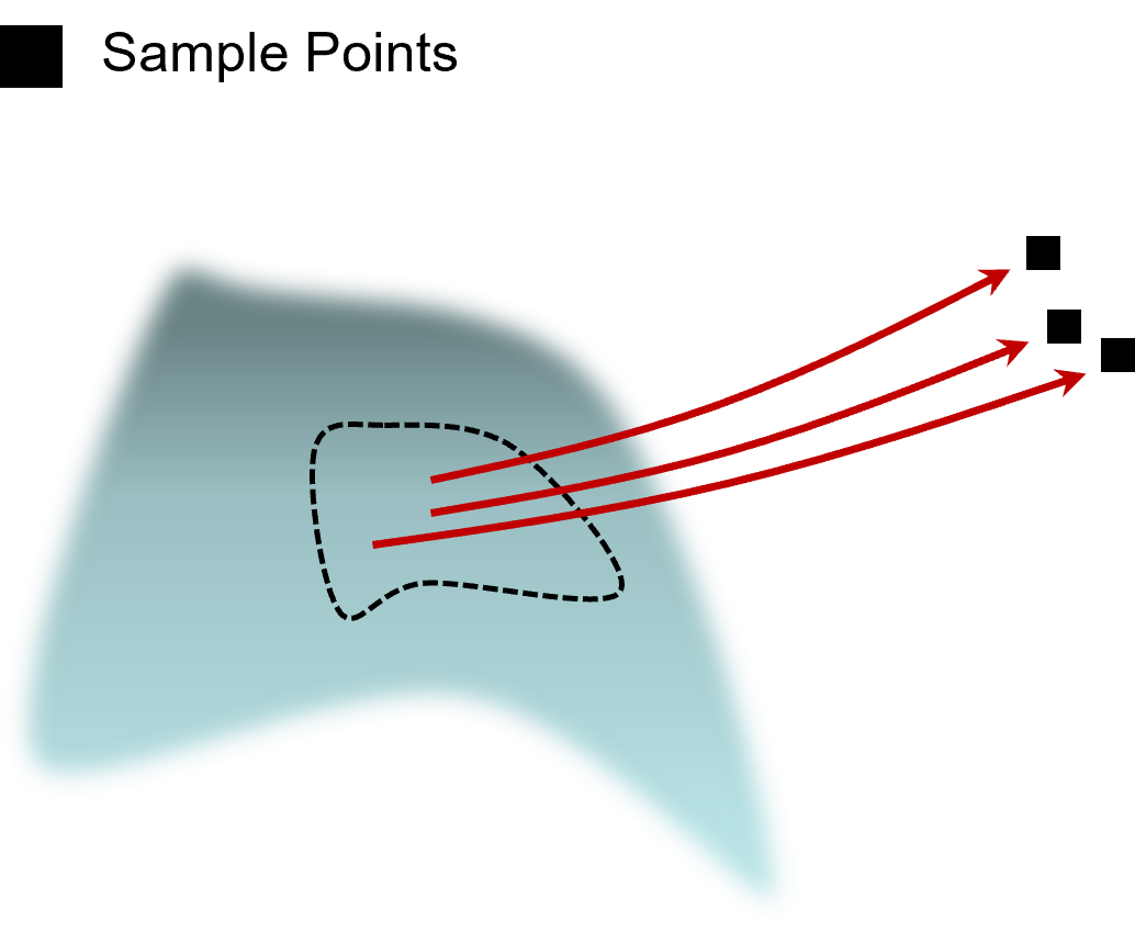
(c) Curve

Figure 4: Sampling methods for different situations.

How to sample. The Poisson flow generation model gives a more effective sampling mode [31].

$$\boldsymbol{x}_{t}=\boldsymbol{x}_{0}+\|\boldsymbol{\varepsilon}_{\boldsymbol{x}}\|(1+\tau)^{m}\boldsymbol{u},\quad t=|\varepsilon_{t}|(1+\tau)^{m}$$ (11)

Among them $(\boldsymbol{\varepsilon}_{\boldsymbol{x}},\varepsilon_{t})\sim\mathcal{N}(\boldsymbol{0},\sigma^{2}\boldsymbol{I}_{(d+1)\times(d+1)}),m\sim U[0,M]$, $u$ is a unit vector uniformly distributed on the d-dimensional unit sphere, and $\tau$, $\sigma$ and $M$ are both constants. This design is much simpler to implement than the inverse cumulative function method, by changing the parameters, this type of sampling method has good generalizability, and the three trajectories we provide also use this type of method. According to Equation (8), we can get the integration of the sampling mode and the $H(x)$ function. For these formulas, it can be regarded as $P(H(\boldsymbol{x}))\propto{\left(1+\|\boldsymbol{x}\|^{2}\right)^{-(d+1)/2}}$, that is, the probability function of $H(x)$ is proportional to the latter. After substituting the Equation (11), we will get

$$\boldsymbol{x}_{t}=\boldsymbol{x}_{0}+t\frac{\|\boldsymbol{\varepsilon}_{\boldsymbol{x}}\|}{|\varepsilon_{t}|}\boldsymbol{u}$$ (12)

$$p(\|\boldsymbol{x}\|)\propto\frac{\|\boldsymbol{x}\|^{d-1}}{\left(1+\|\boldsymbol{x}\|^{2}\right)^{(d+1)/2}}$$

The normal distribution is applicable for $\boldsymbol{\varepsilon}_{\boldsymbol{x}}$ and $\varepsilon_{t}$ in the above expression, which allows us to directly deduce that the probability function of $\frac{\|\boldsymbol{\varepsilon}_{\boldsymbol{x}}\|}{|\varepsilon_{t}|}$ is consistent with the Equation (12) presented below. Similarly, based on this structural property, one can deduce suitable sampling methods for single-sample straight line trajectory force fields and curved force fields, respectively

$$\boldsymbol{x}_{t}=\boldsymbol{x}_{0}+\|\boldsymbol{\varepsilon}_{\boldsymbol{x1}}\|\boldsymbol{u},\quad t=|\varepsilon_{t1}|$$ (13)

$$\boldsymbol{x}_{t}=\boldsymbol{x}_{0}+\|\boldsymbol{\varepsilon}_{\boldsymbol{x2}}\|(1+\tau)^{n}\boldsymbol{u},\quad t=|\varepsilon_{t2}|(1+\tau)^{n}$$

Both $(\boldsymbol{\varepsilon}_{\boldsymbol{x1}},\varepsilon_{t1})$ and $(\boldsymbol{\varepsilon}_{\boldsymbol{x2}},\varepsilon_{t2})$ are drawn from a uniform distribution $U[0,T]$, and the choice of $n$ is determined by the number of curves. Figure 4 visually illustrates the distinction between various sampling methods. It is apparent that the sampling approach is ideal for simple and original distributions. Our goal is to select the most appropriate sampling method to enhance the performance of the model, which is also the direction we have been considering in the preceding derivation. Additionally, as the original distribution pattern of the simple distribution of sampling varies with different force field model designs, it emphasizes the significance of deriving a unified sampling method.

4.4 Conditional Control of Force Field Models

Note that there are various paths for the transformation of any data point. Therefore, we need to theoretically prove a better solution model range, in order to better find the force field model under this conditional constraint. Among them, we assume two trajectories

$$\frac{d\boldsymbol{x}_{t}}{dt}=\boldsymbol{f}_{t}(\boldsymbol{x}_{t}),\quad\frac{d\boldsymbol{y}_{t}}{dt}=\boldsymbol{g}_{t}(\boldsymbol{y}_{t})$$ (14)

And in the conclusion of the stochastic differential equation [27], there is an evolution equation

$$d\boldsymbol{x}_{t}=\left[\boldsymbol{f}_{t}(\boldsymbol{x}_{t})-g_{t}^{2}\nabla_{\boldsymbol{x}_{t}}\log p_{t}(\boldsymbol{x}_{t})\right]dt+g_{t}d\boldsymbol{w}$$ (15)

which can be used to compare the evolutionary differences of different trajectories. First write the evolution equations of the two trajectories, and then perform a type of scaling to get the main difference as

$$-\frac{1}{2}g_{t}^{2}\mathbb{E}_{\boldsymbol{z}}\left[(\nabla_{\boldsymbol{x}_{t}}\log p_{t}(\boldsymbol{x}_{t})-\nabla_{\boldsymbol{y}_{t}}\log q_{t}(\boldsymbol{y}_{t}))\right]$$ (16)

Using this indicator, we can perform a horizontal comparison of the similarities and differences between various types of trajectories during the evolutionary process. This enables us to better identify optimal solutions for a specific type of trajectory under given conditions, and significantly simplifies the search scope for obtaining the desired properties in experiments. It is noteworthy that the mathematical demonstration of the minimum value of this equation is unfeasible due to the existence of the inequality

$$\mathbb{E}_{\boldsymbol{z}}\left[(\nabla_{\boldsymbol{x}_{t}}\log p_{t}(\boldsymbol{x}_{t})-\nabla_{\boldsymbol{y}_{t}}\log q_{t}(\boldsymbol{y}_{t}))\right]\geq 0$$ (17)

is easy to give a counterexample. Consequently, the estimation process necessitates the derivation of an optimal solution predicated on the particular distribution of diverse trajectories.

	Invertible?	Inception↑	FID↓	NFE↓
StyleGAN2-ADA [12]	NO	10.10	2.42	1
Glow [14]	Yes	3.93	48.7	1
DDIM,T=50 [26]	Yes	-	4.82	50
DDIM,T=100 [26]	Yes	-	4.33	100
PGFM [31]	Yes	9.65	2.48	110
Diffusion model with one-sample straight line	Yes	10.12	18.70	24
Diffusion model with multi-sample linear superposition	Yes	12.11	2.33	800
Diffusion model with curve	Yes	9.23	2.65	102
Diffusion model with Gaussian distribution	Yes	9.58	3.06	1000

Table 1: CIFAR-10 sample quality (FID, Inception) and number of function evaluation (NFE).

5 Experiment

Dataset. To identify force field patterns with high speed and high generation quality, we employed the CIFAR-10 dataset, which is a color image dataset that is closer to universal objects. CIFAR-10 was compiled by Hinton’s students Alex Krizhevsky and Ilya Sutskever for pervasive object recognition and contains 10 categories of RGB color images. The images are sized at 32 × 32, and each category has 6000 images. The dataset contains 50000 training images and 10000 test images [22, 17]. We evaluated the diversity and quality of the output images generated by the model using two indicators: Inception [25] (higher is better) and FID scores, which allowed us to effectively assess the model’s performance. Additionally, we assessed the model’s speed by considering the model parameters and training step, to identify a suitable mode of force field construction.

Baselines. We conducted a comparison study of generative models, namely PFGM, GAN [2, 7], and normalized flow [21, 16], under various force field patterns. Our model selection protocol, in line with, involves selecting the checkpoint with the lowest FID score during training at every 50k iterations.

Optimization. In order to draw conclusions with higher confidence, we modified the training samples by randomly flipping and adding noise to construct a mini-batch of size 32. The Adam [13] optimizer is used with an initial learning rate of $10^{-4}$ and the learning rate is multiplied by a factor of 0.8 every 3 epochs.

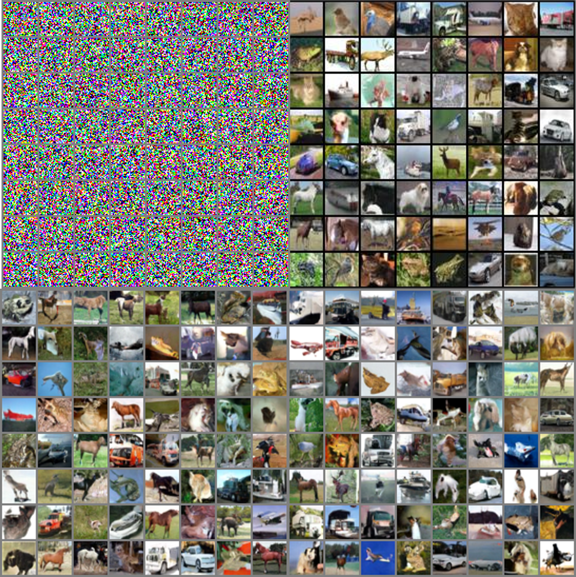
Figure 5: Evolution results of trajectories in several ways on CIFAR-10 datasets.

Results For quantitative evaluation on CIFAR-10, we report the Inception (higher is better) and FID scores (lower is better) in Table 1 second and third column. For speed evaluation on CIFAR-10, we report the number of function evaluation (NFE) [31] in Table 1 forth column.

Our main findings are: (1) The results show that in terms of generation quality, diffusion model with multi-sample linear superposition achieves the best Inception scores and FID scores among the models, which respectively reached 12.11 and 2.33 within 800 steps, and the effect is significantly better than the same type of curve trajectory. (2) The diffusion model utilizing a one-sample straight line has exhibited a notable degree of proficiency within a limited number of iterations. Additionally, the model’s reversibility and insignificant perturbation of the data point distribution engenders a degree of stability throughout the training process.

5.1 Result Analysis

Curved Trajectory vs Multi-Sample Straight Trajectory. Based on our experimental findings, it can be concluded that the multi-sample line model outperforms the curve fitting method in terms of generation quality. We now aim to provide an explanation for this observation. Following the derivation of Equation (5), we have a correlation equation for the original distribution and the sampling result $\boldsymbol{x}_{t}=(\boldsymbol{x}_{T}-\boldsymbol{x}_{0})t+\boldsymbol{x}_{0}$. One can employ the superposition of Taylor expansions to approximate the curve. This method can be applied to fit the sample distribution $\boldsymbol{x}_{T}=\frac{(t-1)(\boldsymbol{x}_{t}-\boldsymbol{x}_{0})}{t^{m}}$ of the curve type. Thus, it can be written as $\boldsymbol{x}_{t}=\sum_{i=1}^{T}(\boldsymbol{x}_{i}-\boldsymbol{x}_{i-1}){t^{i}}$. Using the method of least squares, we can fit the approximate curve obtained by the superposition of Taylor expansions. Therefore, the quality of the final result obtained by the multi-sample straight line trajectory method is superior to that of the curve. Additionally, Figure 3 illustrates the image related to the trajectory movement.

Some problems with Gaussian distribution. In previous works, Gaussian distribution has been predominantly used as the basis for modeling [27, 31]. However, our experiments have revealed certain limitations associated with this approach. Firstly, to obtain the equation about $\boldsymbol{x}_{T}$ through solving differential equations, it is necessary for the variance $\sigma_{t}$ of the Gaussian distribution to satisfy a monotonically increasing function. Secondly, our sampling design imposes strict requirements and is not very compatible with the model design for the Gaussian distribution [31].

5.2 Further Mining Analysis

We conducted a special case analysis for multi-sample straight-line trajectories and discovered interesting properties during training. Similar to the mode collapse in the PFGM proposed in, we found that when the number of straight-line fittings reaches a certain level, the overall quality of the samples generated by the model decreases, and mode collapse occurs. As shown in Figure 6, it can be seen that as the number of fitted curves increases, the quality of the generated image also increases, and the evaluation steps also increase. However, when the number of curves exceeds about 12, the model appears mode collapse phenomenon. To interpret this situation, we can leverage the Green’s function method. Specifically, we assume that the trajectory between two points $\boldsymbol{x}_{0}$ and $\boldsymbol{x}_{1}$ is a straight line, which is only generated for a single point and can be considered as the Green’s function solution. However, when the force field associated with a general distribution is superimposed on the Green’s function, the resulting trajectory is no longer a straight line. This explains why the curve can be approximated by using a multi-sample straight line. When applying the Green’s function method to solve differential equations with high degree, it is possible that the remaining term in the Taylor expansion has a degree that is comparable to the largest term, which can lead to an overall bias in the final function due to the error in the remaining term.

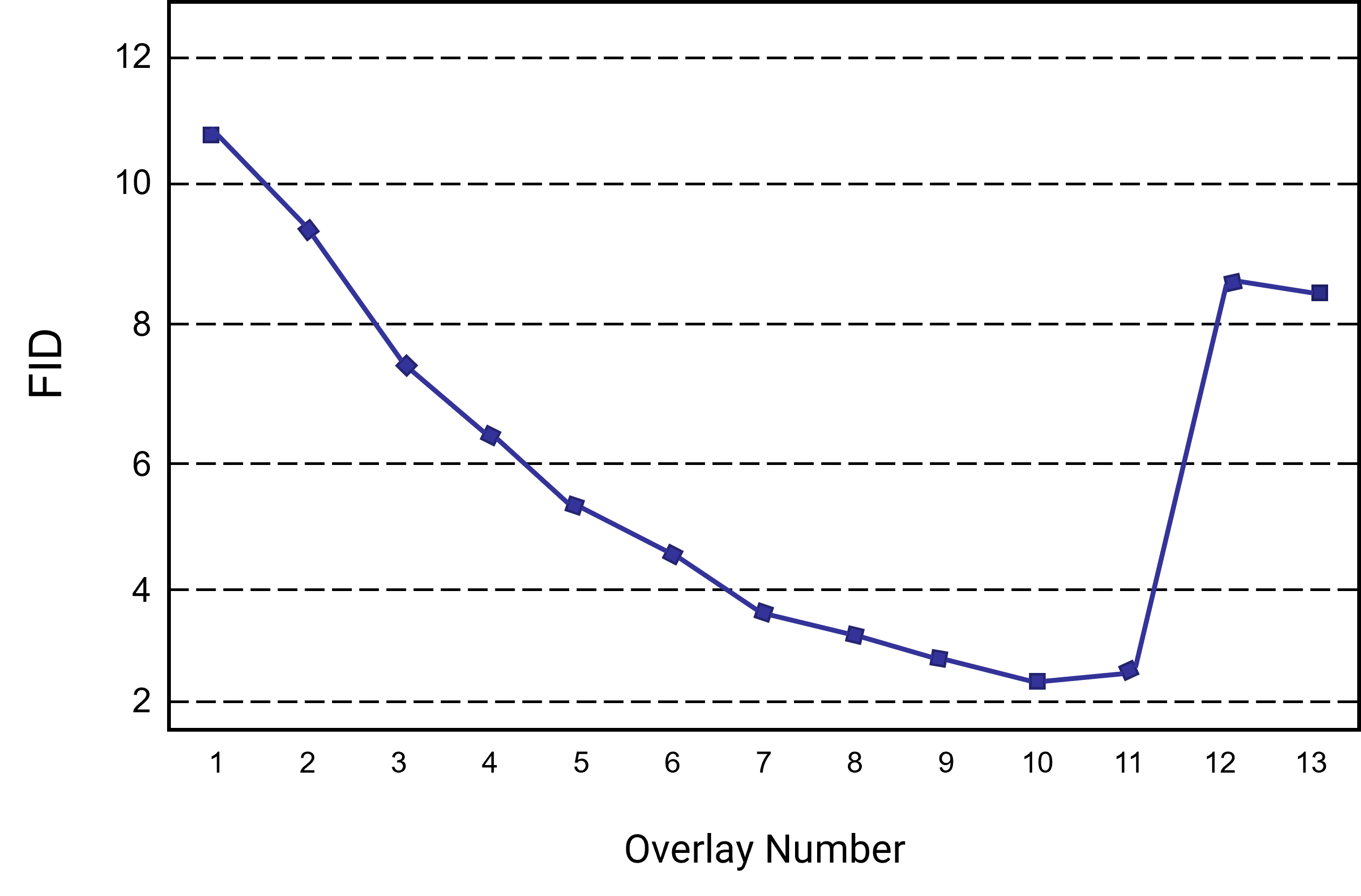
Figure 6: Trajectory overlay number and change of FID.

We have devised a comprehensive metric that takes into account the number of function evaluations and the quality of the samples generated using the FID and Inception metrics. To accomplish this, we first normalize and scale the three metrics, using the z-score method for normalization. The weights of the three metrics are determined based on the distribution of the column, with greater weight assigned to the metric that exhibits greater difference. This approach enables us to analyze the level of mode collapse for different levels of overlapping.

ON	Inception↑	FID↓	NFE↓	Index↑
1	10.27	10.22	46	0.8965
2	10.76	9.51	89	0.8995
3	11.12	7.27	124	0.9118
4	11.25	6.14	189	0.9143
5	11.54	5.12	322	0.9115
6	12.01	4.44	632	0.8941
7	11.79	3.75	689	0.8931
8	12.07	3.42	744	0.8921
9	12.11	2.91	782	0.8924
10	12.11	2.33	800	0.8946

Table 2: Correlation metrics for different amounts of overlap. Among them, ON indicates the number of overlaps, and index is a comprehensive indicator of the three indicators after calculating the weight.

Table 2 presents the results of the comprehensive evaluation of the models in terms of image generation quality and speed. The evaluation considers three aspects of indicators and the final index is calculated by normalizing and combining them using the z-score method. The weights of the indicators are determined based on the properties of the distribution column, giving greater weight to indicators with larger differences. The table shows that the best overall performance is achieved when the number of overlaps is about 4 times. Beyond this point, the overall evaluation drops, possibly due to excessively large training steps. Therefore, when configuring the model, the number of overlaps should be considered from a comprehensive perspective and not set too high. However, to improve performance before mode collapse, the number of overlaps can be increased as much as possible. It is important to note that the assumptions made for the other hyperparameters in this experiment might differ from the settings of your model. Therefore, it is recommended to follow the actual situation as closely as possible.

5.3 Experimental Conclusion

Through the aforementioned experiments and analysis, we have systematically investigated the appropriate force field for building a generative model from an experimental standpoint. We have summarized some principles, such as higher complexity implying more assumptions, which can be difficult to test for compatibility with the target data. Furthermore, more complex trajectories can present higher analytical and experimental difficulties. Multi-point superposition generation can fit complex curves when the basic trajectory is a straight line. However, when the number of fittings is too high, the model may become highly unstable, leading to mode collapse. Therefore, it is crucial to identify the maximum number of generated masses before mode collapse or to aim for a model that can be trained in as few steps as possible, to achieve a higher generation quality.

6 Conclusion

This paper introduces a novel approach to generate force fields based on a theoretical mathematical proof and derivation. Specifically, we leverage the diffusion model to solve the ODE during training and propose three representative model paradigms. Through experimental comparisons with existing methods, we identify force field patterns that exhibit superior generation speed and quality. Additionally, we provide an intuitive analysis and derivation of the results obtained. Moreover, we analyze the essential principles underlying the construction of such force fields, thereby offering valuable insights for future research in this area.

APPENDIX

7 Proofs

7.1 Derivation of Objective Function

In Equation (6), we have such a conclusion:

$$\mathbb{E}_{\boldsymbol{x}_{0},\boldsymbol{x}_{t}\sim d_{t}(\boldsymbol{x}_{t}|\boldsymbol{x}_{0})d_{0}(\boldsymbol{x}_{0})}\left[\left\|\boldsymbol{s}_{\boldsymbol{\theta}}(\boldsymbol{x}_{t},t)-\boldsymbol{F}_{t}(\boldsymbol{x}_{t}|\boldsymbol{x}_{0})\right\|^{2}\right]$$

The source of the derivation of this equation is firstly the solution to the H(x) introduced above. For the transfer equation, $\frac{\partial}{\partial t}d_{t}(\boldsymbol{x}_{t})=-\nabla_{\boldsymbol{x}_{t}}\cdot(\boldsymbol{F}_{t}(\boldsymbol{x}_{t})d_{t}(\boldsymbol{x}_{t}))$ can be rewritten as

$$\frac{\partial}{\partial t}d_{t}(\boldsymbol{x}_{t}|\boldsymbol{x}_{0})+\nabla_{\boldsymbol{x}_{t}}d_{t}(\boldsymbol{x}_{t}|\boldsymbol{x}_{0})\cdot\boldsymbol{f}_{t}(\boldsymbol{x}_{t}|\boldsymbol{x}_{0})+d_{t}(\boldsymbol{x}_{t}|\boldsymbol{x}_{0})\nabla_{\boldsymbol{x}_{t}}\cdot\boldsymbol{F}_{t}(\boldsymbol{x}_{t}|\boldsymbol{x}_{0})=0$$

At this point, the problem is transformed into solving a class of partial differential equations. For a particular trajectory of the data, $\boldsymbol{F}_{t}$ can be transformed into a relative quantity of $\boldsymbol{x}_{t}$. Therefore, the overall expression can be simplified as

$$\frac{d}{dt}d_{t}(\boldsymbol{x}_{t}|\boldsymbol{x}_{0})+d_{t}(\boldsymbol{x}_{t}|\boldsymbol{x}_{0})\nabla_{\boldsymbol{x}_{t}}\cdot\boldsymbol{F}_{t}(\boldsymbol{x}_{t}|\boldsymbol{x}_{0})=0$$

For such a class of equations that have been transformed into ordinary differential equations, they can be directly brought into the formula to solve:

$$d_{t}(\boldsymbol{x}_{t}|\boldsymbol{x}_{0})=C\exp\left(\int_{t}^{T}\nabla_{\boldsymbol{x}_{s}}\cdot\boldsymbol{F}_{s}(\boldsymbol{x}_{s}|\boldsymbol{x}_{0})ds\right)$$

$$d_{t}(\boldsymbol{x}_{t}|\boldsymbol{x}_{0})=d_{T}(\boldsymbol{x}_{T})\exp\left(\int_{t}^{T}\nabla_{\boldsymbol{x}_{s}}\cdot\boldsymbol{F}_{s}(\boldsymbol{x}_{s}|\boldsymbol{x}_{0})ds\right)$$

where $\boldsymbol{x}_{T}$ is the distribution sampled by the last sampling mode. Afterwards, we bring such a trajectory mode into it, and then we can simplify and get the related expression to find that: $\boldsymbol{H}(t,0;\boldsymbol{x}_{t},\boldsymbol{x}_{0})=p_{t}(\boldsymbol{x}_{t}|\boldsymbol{x}_{0})\boldsymbol{F}_{t}(\boldsymbol{x}_{t}|\boldsymbol{x}_{0})$. Guided by the $H$ function, we can find out by adding it to the constraints of the differential equation

$$\boldsymbol{v}_{1}(t,\boldsymbol{x}_{t})= \,\int d_{t}(\boldsymbol{x}_{t}|\boldsymbol{x}_{0})d_{0}(\boldsymbol{x}_{0})d\boldsymbol{x}_{0}=d_{t}(\boldsymbol{x}_{t})$$

$$\boldsymbol{v}_{t}(t,\boldsymbol{x}_{t})= \,\int\boldsymbol{F}_{t}(\boldsymbol{x}_{t}|\boldsymbol{x}_{0})d_{t}(\boldsymbol{x}_{t}|\boldsymbol{x}_{0})d_{0}(\boldsymbol{x}_{0})d\boldsymbol{x}_{0}$$

Accordingly, using the definition of the expectation formula, we can derive the objective function we need

$$\boldsymbol{F}_{t}(\boldsymbol{x}_{t})= \,\frac{\boldsymbol{v}_{t}(t,\boldsymbol{x}_{t})}{\boldsymbol{v}_{1}(t,\boldsymbol{x}_{t})}\ =\frac{1}{d_{t}(\boldsymbol{x}_{t})}\int\boldsymbol{F}_{t}(\boldsymbol{x}_{t}|\boldsymbol{x}_{0}){d_{t}(\boldsymbol{x}_{t}|\boldsymbol{x}_{0})d_{0}(\boldsymbol{x}_{0})}d\boldsymbol{x}_{0}$$

$$= \,\int d_{t}(\boldsymbol{x}_{0}|\boldsymbol{x}_{t})\boldsymbol{f}_{t}(\boldsymbol{x}_{t}|\boldsymbol{x}_{0})d\boldsymbol{x}_{0}\ =\mathbb{E}_{\boldsymbol{x}_{0}\sim d_{t}(\boldsymbol{x}_{0}|\boldsymbol{x}_{t})}\left[\boldsymbol{F}_{t}(\boldsymbol{x}_{t}|\boldsymbol{x}_{0})\right]$$

7.2 Details of the Sampling Method

The Poisson flow generation model gives a more effective sampling mode in Equation (11). In this section we will derivate this whole process. According to $(\boldsymbol{\varepsilon}_{\boldsymbol{x}},\varepsilon_{t})\sim\mathcal{N}(\boldsymbol{0},\boldsymbol{I}_{(d+1)\times(d+1)})$, we can get

$$p(\|\boldsymbol{\varepsilon}_{\boldsymbol{x}}\|)\propto\|\boldsymbol{\varepsilon}_{\boldsymbol{x}}\|^{d-1}e^{-\|\boldsymbol{\varepsilon}_{\boldsymbol{x}}\|^{2}/2},\quad p(|\varepsilon_{t}|)\propto e^{-|\varepsilon_{t}|^{2}/2}$$

let $r=\frac{\|\boldsymbol{\varepsilon}_{\boldsymbol{x}}\|}{|\varepsilon_{t}|}$, it can release

$$p(r)dr= \,\mathbb{E}_{|\varepsilon_{t}|\sim p(|\varepsilon_{t}|)}\big{[}p(\|\boldsymbol{\varepsilon}_{\boldsymbol{x}}{=r|\varepsilon_{t}|})d({r|\varepsilon_{t}|})\big{]}\propto\mathbb{E}_{|\varepsilon_{t}|\sim p(|\varepsilon_{t}|)}\big{[}r^{d-1}|\varepsilon_{t}|^{d}e^{-r^{2}|\varepsilon_{t}|^{2}/2}dr\big{]}\propto$$

$$\int_{0}^{\infty}r^{d-1}|\varepsilon_{t}|^{d}e^{-r^{2}|\varepsilon_{t}|^{2}/2}e^{-|\varepsilon_{t}|^{2}/2}d|\varepsilon_{t}|dr= \,\int_{0}^{\infty}r^{d-1}|\varepsilon_{t}|^{d}e^{-(r^{2}+1)|\varepsilon_{t}|^{2}/2}d|\varepsilon_{t}|dr$$

$$= \,\frac{r^{d-1}}{(1+r^{2})^{(d+1)/2}}\int_{0}^{\infty}k^{d}e^{-k^{2}/2}dsdr\quad\left(\text{let}~{}k=|\varepsilon_{t}|\sqrt{r^{2}+1}\right)$$

Finally, the conclusion of Equation (12) is obvious.

8 Results of Experiments

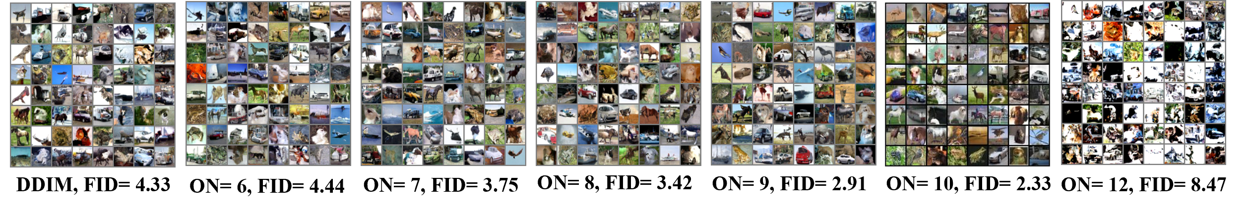
Figure 7: Generated results in different situations.

The outcomes of several techniques alluded to in the primary discourse are depicted in Figure 1, revealing that the manifestation of mode collapse evinced at 12 trajectories diverges from other instances.

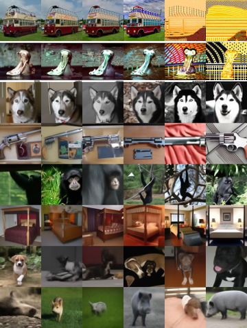
Figure 8: Evolution of results on ImageNet-64 (using the best performing force field model).

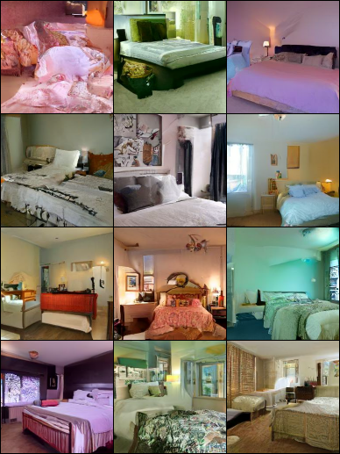
Figure 9: LSUN bedroom 256×256 samples using PFGM.

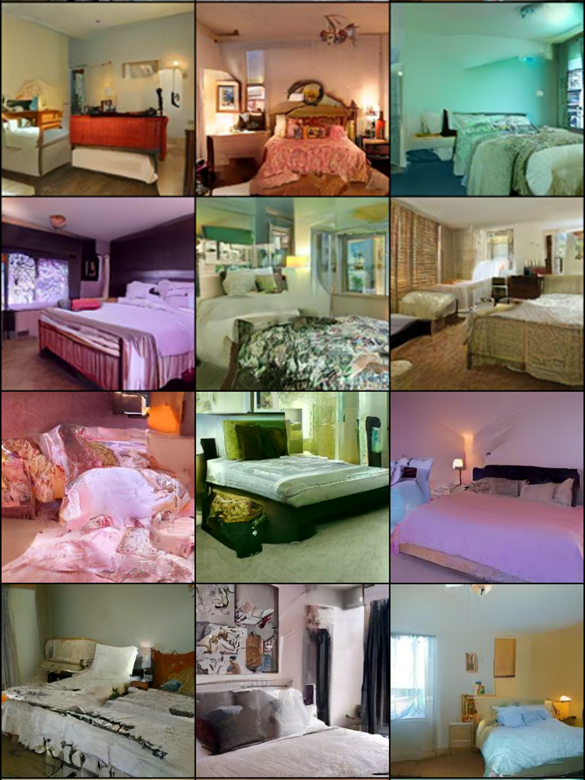
Figure 10: LSUN bedroom 256×256 samples using best performing force field model.

References

- [1] Kartik Ahuja, Jason Hartford, and Yoshua Bengio. Properties from mechanisms: an equivariance perspective on identifiable representation learning. arXiv preprint arXiv:2110.15796, 2021.
- [2] Andrew Brock, Jeff Donahue, and Karen Simonyan. Large scale gan training for high fidelity natural image synthesis. arXiv preprint arXiv:1809.11096, 2018.
- [3] Tom Brown, Benjamin Mann, Nick Ryder, Melanie Subbiah, Jared D Kaplan, Prafulla Dhariwal, Arvind Neelakantan, Pranav Shyam, Girish Sastry, Amanda Askell, et al. Language models are few-shot learners. Advances in neural information processing systems, 33:1877–1901, 2020.
- [4] P Kingma Diederik, Max Welling, et al. Auto-encoding variational bayes. In Proceedings of the International Conference on Learning Representations (ICLR), volume 1, 2014.
- [5] Laurent Dinh, Jascha Sohl-Dickstein, and Samy Bengio. Density estimation using real nvp. arXiv preprint arXiv:1605.08803, 2016.
- [6] John R Dormand and Peter J Prince. A family of embedded runge-kutta formulae. Journal of computational and applied mathematics, 6(1):19–26, 1980.
- [7] Ishaan Gulrajani, Faruk Ahmed, Martin Arjovsky, Vincent Dumoulin, and Aaron C Courville. Improved training of wasserstein gans. Advances in neural information processing systems, 30, 2017.
- [8] Martin Heusel, Hubert Ramsauer, Thomas Unterthiner, Bernhard Nessler, and Sepp Hochreiter. Gans trained by a two time-scale update rule converge to a local nash equilibrium. Advances in neural information processing systems, 30, 2017.
- [9] Jonathan Ho, Xi Chen, Aravind Srinivas, Yan Duan, and Pieter Abbeel. Flow++: Improving flow-based generative models with variational dequantization and architecture design. In International Conference on Machine Learning, pages 2722–2730. PMLR, 2019.
- [10] Jonathan Ho, Ajay Jain, and Pieter Abbeel. Denoising diffusion probabilistic models. Advances in Neural Information Processing Systems, 33:6840–6851, 2020.
- [11] Vivek Jayaram and John Thickstun. Parallel and flexible sampling from autoregressive models via langevin dynamics. In International Conference on Machine Learning, pages 4807–4818. PMLR, 2021.
- [12] Tero Karras, Miika Aittala, Janne Hellsten, Samuli Laine, Jaakko Lehtinen, and Timo Aila. Training generative adversarial networks with limited data. Advances in neural information processing systems, 33:12104–12114, 2020.
- [13] Diederik P Kingma and Jimmy Ba. Adam: A method for stochastic optimization. arXiv preprint arXiv:1412.6980, 2014.
- [14] Durk P Kingma and Prafulla Dhariwal. Glow: Generative flow with invertible 1x1 convolutions. Advances in neural information processing systems, 31, 2018.
- [15] Durk P Kingma, Shakir Mohamed, Danilo Jimenez Rezende, and Max Welling. Semi-supervised learning with deep generative models. Advances in neural information processing systems, 27, 2014.
- [16] Ivan Kobyzev, Simon JD Prince, and Marcus A Brubaker. Normalizing flows: An introduction and review of current methods. IEEE transactions on pattern analysis and machine intelligence, 43(11):3964–3979, 2020.
- [17] Alex Krizhevsky, Geoffrey Hinton, et al. Learning multiple layers of features from tiny images. , 2009.
- [18] Yaron Lipman, Ricky TQ Chen, Heli Ben-Hamu, Maximilian Nickel, and Matt Le. Flow matching for generative modeling. arXiv preprint arXiv:2210.02747, 2022.
- [19] Qiao Liu, Jiaze Xu, Rui Jiang, and Wing Hung Wong. Density estimation using deep generative neural networks. Proceedings of the National Academy of Sciences, 118(15):e2101344118, 2021.
- [20] Alexander Quinn Nichol and Prafulla Dhariwal. Improved denoising diffusion probabilistic models. In International Conference on Machine Learning, pages 8162–8171. PMLR, 2021.
- [21] George Papamakarios, Eric Nalisnick, Danilo Jimenez Rezende, Shakir Mohamed, and Balaji Lakshminarayanan. Normalizing flows for probabilistic modeling and inference. The Journal of Machine Learning Research, 22(1):2617–2680, 2021.
- [22] Benjamin Recht, Rebecca Roelofs, Ludwig Schmidt, and Vaishaal Shankar. Do cifar-10 classifiers generalize to cifar-10? arXiv preprint arXiv:1806.00451, 2018.
- [23] Danilo Rezende and Shakir Mohamed. Variational inference with normalizing flows. In International conference on machine learning, pages 1530–1538. PMLR, 2015.
- [24] Hannes Risken and Hannes Risken. Solutions of the kramers equation. The Fokker-Planck Equation: Methods of Solution and Applications, pages 229–275, 1984.
- [25] Tim Salimans, Ian Goodfellow, Wojciech Zaremba, Vicki Cheung, Alec Radford, and Xi Chen. Improved techniques for training gans. Advances in neural information processing systems, 29, 2016.
- [26] Jiaming Song, Chenlin Meng, and Stefano Ermon. Denoising diffusion implicit models. arXiv preprint arXiv:2010.02502, 2020.
- [27] Yang Song, Jascha Sohl-Dickstein, Diederik P Kingma, Abhishek Kumar, Stefano Ermon, and Ben Poole. Score-based generative modeling through stochastic differential equations. arXiv preprint arXiv:2011.13456, 2020.
- [28] Thomas Unterthiner, Bernhard Nessler, Calvin Seward, Günter Klambauer, Martin Heusel, Hubert Ramsauer, and Sepp Hochreiter. Coulomb gans: Provably optimal nash equilibria via potential fields. arXiv preprint arXiv:1708.08819, 2017.
- [29] Arash Vahdat, Karsten Kreis, and Jan Kautz. Score-based generative modeling in latent space. 2021. arXiv preprint arXiv:2106.05931, 2021.
- [30] Nicolaas G Van Kampen. Stochastic differential equations. Physics reports, 24(3):171–228, 1976.
- [31] Yilun Xu, Ziming Liu, Max Tegmark, and Tommi Jaakkola. Poisson flow generative models. arXiv preprint arXiv:2209.11178, 2022.
- [32] Ling Yang, Zhilong Zhang, Yang Song, Shenda Hong, Runsheng Xu, Yue Zhao, Yingxia Shao, Wentao Zhang, Bin Cui, and Ming-Hsuan Yang. Diffusion models: A comprehensive survey of methods and applications. arXiv preprint arXiv:2209.00796, 2022.