Online Neural Path Guiding with Normalized Anisotropic Spherical Gaussians

Abstract.

The variance reduction efficiency of physically-based rendering is heavily affected by the adopted importance sampling technique. In this paper we propose a novel online framework to learn the spatial-varying density model with a single small neural network using stochastic ray samples. To achieve this task, we propose a novel closed-form density model called the Normalized Anisotropic Spherical Gaussian mixture, that can express complex irradiance fields with a small number of parameters. Our framework learns the distribution in a progressive manner and does not need any warm-up phases. Due to the compact and expressive representation of our density model, our framework can be implemented entirely on the GPU, allowing it to produce high quality images with limited computational resources. The result shows our framework achieves better guiding efficiency compared to state-of-the-art online learning path guiding methods.

Reference	(a) Ours	(b) (Müller, 2019)	(c) Path Tracing
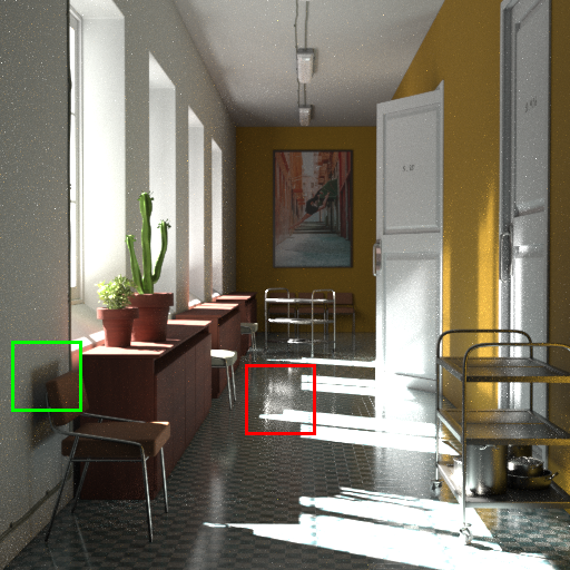
MAPE:	0.058	0.063	0.120

Figure 1. Our framework allows a GPU path tracer to effectively learn irradiance distribution for every shading point with a small neural network online. We compare equal-time rendering results of our framework (a) with (Müller, 2019) (b) and path tracing with next event estimation (c). Our framework achieves efficient neural path guiding that conventional PC can afford.

1. Introduction

Unbiased physically-based rendering (PBR) is achieved by launching light transport simulation to solve the rendering equation with Monte Carlo methods. Over the past decades, unidirectional path tracing has become the dominant method of PBR in the film and design industries because of its flexibility and simplicity. To reduce variance of Monte Carlo integral efficiently, many importance sampling methods have been proposed (e.g., (Veach, 1998; Ureña et al., 2013; Hart et al., 2020)). However, currently only some components in rendering equation (typically, the BSDF term, or direct lighting) can be importance-sampled. When indirect lighting is dominant, the sampling efficiency becomes poor.

Path guiding is a promising genre of importance sampling approaches to overcome the challenge (Vorba et al., 2014; Müller et al., 2017). A path guiding method usually learns a distribution model over the 3D scene that fits the rendering equation closer, either during the rendering process (online) or with precomputation (offline). Then, the path tracer can importance-sample the scattering directions based on the learned distribution. Previous approaches such as (Vorba et al., 2014; Müller et al., 2017) partition the 3D space and approximate the incident radiance of each zone using statistical models (typically, histogram-based model or expectation-maximization) instead of modelling the whole product of the rendering equation, which fails to represent per-shading-point distribution.

Recently, an emerging direction to learn the per-shading-point product distribution of rendering equation is to model such spatially varying distribution with neural networks (Müller et al., 2020; Zhu et al., 2021a, b). Ideally, an explicit model that directly learns the per-shading-point product distribution is desired but this has been difficult due to (1) the lack of a representation that can reconstruct both high and low frequency features with small number of parameters and (2) a closed-form density model that provides an analytical solution for integrating the distribution for normalization. As a result, existing models either learn an implicit model that only provides a mapping between uniform distribution and the shading-point product distribution but with expensive computation  (Müller et al., 2020); learn a coarse, low resolution distribution with limited accuracy (Zhu et al., 2021a); or require costly offline precomputation (Zhu et al., 2021b).

In this paper, we propose a novel neural-network-based path guiding framework, which learns an explicit spatial-varying distribution of irradiance over the surfaces in a 3D scene. The key insight of our framework is a novel closed-form normalized density model called the Normalized Anisotropic Spherical Gaussian mixture (NASG), that can be effectively trained with sparse training samples. Due to the simplicity and expressiveness of our density model, its parameters can be efficiently learned online via a tiny, multiple layer perceptron (MLP)-based neural network.

Our framework is robust to handle a variety of lighting setups ranging from normal indirect-illuminated scenes to caustics from very narrow light sources. With our closed-form density model, we are able to not only guide sampling of indirect lighting more effectively, but also achieve more efficient direct lighting sampling by blending samples with next event estimation (NEE). We propose the corresponding training workflow including specialized loss function and online acquisition of training samples. As our network can be easily stored and executed in parallel on a GPU, by integrating our neural network with a wavefront path tracer, we are able to implement a high-performance neural-guided unidirectional path tracer on a single GPU, making neural-guiding affordable for conventional personal computers. Our system can produce much higher quality results compared to the state-of-the-art methods given the same computational resources.

The contribution of this paper can be summarized as:

• Normalized Anisotropic Spherical Gaussian mixture, a novel density model that can be used to learn spatial-varying density distribution effectively for path tracing, and

• a novel, lightweight, online neural path guiding framework, using only one small neural network that can be integrated with either CPU or GPU-based conventional product path tracers.

2. Related Work

2.1. Physically-based Rendering and Importance Sampling

The radiance of a shading point can be calculated using the Rendering equation (Kajiya, 1986):

(1) $$L(\mathbf{x})=L_{e}+\int_{\Omega}f_{s}(\mathbf{x},\omega_{i},\omega_{o})L_{i}|\cos\theta|d\omega_{i}$$

where $\mathbf{x}$ is the shading point, and its irradiance towards direction $\omega_{o}$ is the integral over the solid angles, which is a product of bidirectional scattering coefficient $f_{s}$, incident light $L_{i}$, and the geometry factor $cos\theta$. In 3D scenes, due to light bounce, $L_{i}$ forms another integral as Eq. (1) at the point where it originates from. This makes the problem highly complex, and no analytical solution can be formed.

The goal of a path tracer is to solve the rendering equation via the Monte Carlo method, which draws a random direction sample $\omega_{i}^{\prime}$, and calculates a product:

(2) $$L(\mathbf{x})\approx L_{e}+\frac{1}{N}\sum_{k}^{N}\frac{f_{s}(\mathbf{x},\omega_{ik},\omega_{o})L_{ik}|\cos\theta|}{p(\mathbf{x},\omega_{ik})},$$

where $p(\mathbf{x},\omega_{ik})$ is the probability density function (PDF) of the samples. The variance reduction efficiency of path tracing is strongly affected by importance sampling techniques. Early works show that following the BSDF distribution $f_{s}$ can greatly improve the sampling efficiency. Next Event Estimation (NEE) can also greatly improve sampling efficiency for direct lighting, which can be considered as importance sampling of $L_{i}$. Veach et al. (1998) propose Multiple Importance Sampling (MIS) which is a crucial method to combine different distributions to achieve better efficiency, and is widely used in current path tracers. Recent researches focus on applying importance sampling to more challenging tasks. Droske et al. (2015) develop a technique called manifold next event estimation (MNEE) to specifically explore the light path with refractive chains, which greatly improves the sampling efficiency of caustics with unidirectional path tracing. Zeltner et al. (2020) generalize MNEE to other diffuse-specular-diffuse (SDS) rendering scenarios. Heitz et al. (2016b) address the energy loss in microfacet scattering models through importance sampling. Conty Estevez and Kulla (2018) and Moreau et al. (2022) propose algorithms with BVH-based structures to importance sample light sources in many-light scenes.

There still exist complex scenes where no trivial unbiased approach is applicable. Misso et al. (2022) propose to adopt biased estimators (e.g., (Hachisuka and Jensen, 2009)) with debiasing algorithm, and West et al. (2022) propose an algorithm to leverage sampling methods with marginal PDFs.

Although many components of rendering equation can be importance sampled, a universal importance sampling technique for the whole product of the rendering equation is long awaited. Path guiding, which is an approach that we describe next, is a promising direction to address this problem.

2.2. Path Guiding

Path guiding methods aim to find sufficient approximation of the product, so that better importance sampling following the global illumination distribution (rather than local BSDF distribution) becomes possible. Jensen (1995) proposes a pioneering work of path guiding. Vorba et al. (2014) fits a Gaussian mixture to model a distribution estimated by an explicit photon tracing pass. Müller et al. (2017; 2019) propose the “Practical Path Guiding (PPG)” algorithm that models the distribution using the SD-tree representation. PPG is already adopted by several production renderers. These techniques share the same idea of partitioning the space and progressively learning the spatially varying indirect lighting distribution. Recent research shows that good path guiding requires a proper blending weight between BSDF and product-driven distributions (Müller et al., 2020), and the learned distribution should be variance-aware since the samples are not in a zero-variance manner (Rath et al., 2020). These findings help to achieve a more robust path guiding framework.

Despite general path guiding focuses on importance sampling of the entire environment, recent works also guide paths for specific light sources. Li et al. (2022) achieve efficient sampling for caustics by first collecting several important paths and then extending them with a chain of spherical Gaussians; however this method is difficult to be extended to learn general distributions, since it leverages the assumption that such caustics distribution is narrow. Zhu et al. (2021a) propose to use an offline-trained neural network to efficiently sample complex lamps. Despite the improved efficiency in sampling, it requires to offline-train a U-Net for more than 10 hours for one light source, which is not practical in many production scenarios. Also, the estimated distribution is only a $16\times 16$ 2D map, which is not sufficient for representing general indirect lighting distributions: a much higher resolution is required for robustly guiding over the whole 3D scene (for instance, PPG’s quad-tree approach can represent a resolution of $2^{16}\times 2^{16}$).

Recently, learning-based online path guiding has been studied: Müller et al. (2020) utilize normalizing flow (Kobyzev et al., 2021) to model the light distribution. However, with normalizing flow, each sample/density evaluation requires a full forward pass of multiple neural networks, which introduces heavy computation costs. Moreover, the training process requires dense usage of differentiable transforms which makes the training slower than regular neural networks; actually, Müller et al.(2020) use two GPUs specifically for its neural network computation along with the CPU-based path tracing implementation, and still the sampling speed is only 1/4 of PPG. Our work, in contrast, proposes to use an explicitly parameterized density distribution model in closed-form that can be learned using a small MLP. The neural network is utilized to generate the closed-form distribution model, rather than actual samples; therefore we are able to freely generate samples or evaluate the density after a single forward pass. With careful implementation, we show that our method can reach a similar sampling rate with PPG, while the result has lower variance.

2.3. GPU Path Tracing

GPU path tracing has gained significant attention in recent years due to its ability to sample substantially more pixels concurrently and its focus on performance. Many recent research achievements focus on making real-time path tracing possible (e.g., (Lin et al., 2022; Bitterli et al., 2020; Ouyang et al., 2021; Müller et al., 2021; Chaitanya et al., 2017)), while GPU-based production renderers leverage GPU to render fully converged, noise-free results faster (e.g., (Autodesk, 2023; Maxon, 2023; OTOY, 2023; Chaos, 2023)). Compared to CPU architecture, GPU requires more sophisticated programming design for better concurrency to hide its large memory latency. A general idea for this is ray reordering (Meister et al., 2020; Lü et al., 2017). (Laine et al., 2013) proposed a new architecture that splits full path tracing computation into stages (small kernels) and processes threads in the same stage to maximize performance. Recently (Zheng et al., 2022) proposes a more sophisticated framework for GPU path tracing which leverages run-time compilation for high performance and flexible implementation. While there are several GPU-based renderer products available, and it is proved that path guiding can improve the sampling efficiency (e.g., many CPU-based rendering products such as (SideFX, 2022; Pixar, 2023), have implemented a path guiding integrator), there lacks GPU-based path guiding implementation in these products. This is because existing path guiding approaches are designed for CPUs and care little about GPU specifications, meanwhile the overhead is rather high in GPU context. Our work provides a low-cost per-sample-point path guiding option for GPU-based path tracers.

2.4. Density Models

Parameteric density models are well explored in statistics. Exponential distribution is a representative family, among which Gaussian mixture is the most widely used density model. In physically-based rendering context, its variant, spherical Gaussian (SG), is proposed (Wang et al., 2009) and applied for representing the light distribution. While the shape of univariate Gaussian distribution is limited, multivariate Gaussian distributions solve this problem by introducing the variance matrix. Following this idea, much effort has been put to for density models in the solid angle domain. Xu et al. (2013) proposes anisotropic spherical Gaussian model to achieve a larger variety of shapes, however there is no analytic solution for its integral, which is problematic for normalization. Heitz et al. (2016a) propose another anisotripic model that has a closed-form expression called linear transform consines (LTC), however the integral of LTC requires computation of inverse matrix and it requires in total 12 scalars to parameterize a component. Dodik et al. (2022) parameterize anisotropic distributions with fewer parameters, however it maps the tangent space circle to a square while the sampling applies to the whole 2D plane so that the PDF is only an approximation. This results in a non-trivial sampling process with discarding samples, which limits the sampling efficiency (especially when representing a large, low-frequency area with even numbers). Bivariate Gaussian used in (Vorba et al., 2014) shares a similar limitation.

Another family of density models widely adopted in the rendering context is the polynomial family, among which the spherical harmonics is the most commonly used model. Polynomial models have been widely used in graphics (Sloan et al., 2002; Moon et al., 2016). They can be easily mapped to unit spheres to be converted into a solid angle representation. On the other hand, when the spectrum is composed of many frequencies, a high dimensional vector is needed for representing the distribution. Furthermore, there is no good approach to importance sample a polynomial distribution. These were the main challenges in our pilot study that made us give up adopting them for our path guiding scheme.

Learning-based density models are drawing more attention recently (Müller et al., 2020; Gilboa et al., 2021). The model by normalizing flow successfully learns complex distributions (Müller et al., 2020) but suffers from the implicitness and heavy computation as mentioned earlier.

“Marginalizable Density Model Approximation (MDMA)” (Gilboa et al., 2021) is proposed as a closed-form learning-based density model, which is essentially a linear combination of multiple sets of 1D distributions. The authors show that closed-form normalization is an essential factor for learning density models: inspired by their work, we propose such a model for our application.

3. Overview

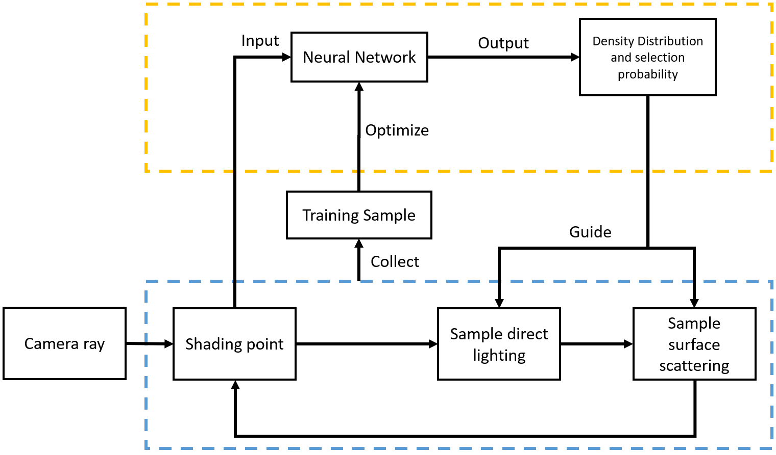
Figure 2. The overview of our framework. Blue part is the computation of a classic path tracer. Yellow part shows how we learn the light distribution with neural network and use the estimated explicit density model to guide further sampling.

The goal of our work is to model the density distribution of the product over unit sphere for every unique shading point $\mathbf{x}$, so that $L(\mathbf{x})$ can be fully importance-sampled (see § 4 for the details of our proposed density model). As shown in Fig. 2, on top of a standard path tracer with next event estimation (direct lighting) and scattering sampling (global illumination), we progressively train a neural network that outputs the parameters for our density model using the rendering samples. The inputs to the network during runtime include the position of the shading point, its normal vector, and the outgoing direction of the light. Using the estimated density model, the ray is sampled at each reflection point to eventually compute the color at the shading point $\mathbf{x}$.

4. Normalized Density Model

In this section, we describe about our proposed density model that we call the Normalized Anisotropic Spherical Gaussian mixture (NASG), that allows us to progressively learn the light distribution at each shading point. We first describe the background by reviewing existing normalized density models that inspired our model in § 4.1. We then describe about our model in § 4.2.

4.1. Background

One of the main requirements for progressively learning a distribution with neural networks is that the models must be normalizable, meaning that the distribution must be able to be integrated to 1. For this purpose, it is beneficial to have a closed-form solution for the integration of the model.

Marginalizable Density Model Approximation

Gilboa et al. (2021) proposes Marginable Density Model Approximation (MDMA) which can be effectively optimized via deep learning. A bivariate dimensional density distribution can be modeled as:

(3) $$D(x,y)=\sum_{i,j}A_{ij}\phi_{1i}(x)\phi_{2j}(y)$$

where $\phi_{1i}$ and $\phi_{2j}$ are 1D normalized distributions, and the $A_{ij}$ are normalized coefficients that sum to 1.

In practice, the 1D distributions in MDMA can be piece-wise linear or piece-wise quadratic models, however, with limited number of components, MDMA can only learn a coarse distribution. Therefore it only gives poor results for distributions with high-frequencies. Despite the accuracy limitation, MDMA works well in learning distribution from sparse noisy samples, compared with unnormalized models (e.g., polynomial model, spherical harmonics): during training, samples with high energy can lower contribution of other areas, and eventually the training converges. This feature is crucial in learning distribution for path guiding.

Normalized Gaussian Mixtures

Normalized Gaussian mixtures can address the accuracy limitation of MDMA:

(4) $$D(\bm{\mathbf{x}})=\sum_{i}^{N}A_{i}\frac{G_{i}(\bm{\mathbf{x}};\theta_{i})}{K_{i}},$$

where $G_{i}(\bm{\mathbf{x}};\theta_{i})$ are Gaussian distributions parameterized by $\theta_{i}$, $K_{i}$ is a normalizing factor, $A_{i}$ are normalized weights of Gaussians such that $\sum_{i}A_{i}=1$. Gaussian mixtures are highly expressive and also easily normalizable: we look into two common Gaussian distributions that can represent spherical distributions that we need for modeling the lighting: spherical Gaussian and anisotropic spherical Gaussian.

Spherical Gaussian

Spherical Gaussian (SG) is a variant of univariate Gaussian function defined in the spherical domain:

(5) $$G(\mathbf{v};\bm{\mu},\lambda)=\exp(\lambda(\bm{\mu}\cdot\mathbf{v}-1)),$$

where $\mu$ is the lobe axis and $\lambda$ is a parameter that controls the “sharpness” of the distribution. The normalizing term of an SG can be computed by:

(6) $$K=\int_{S^{2}}G(\mathbf{v};\bm{\mu},\lambda)d\omega=\frac{2\pi}{\lambda}(1-e^{-2\lambda}).$$

As SG is defined in the spherical domain and is suitable for representing all-frequency light distribution at each sample point, Gaussian mixture models based on SG has been applied for representing the light map for PRT (Wang et al., 2009). However, SG is an isotropic univariate model, hence less expressive; e.g., it cannot represent anisotropic distributions.

Anisotropic Spherical Gaussian

To model anisotropic distributions, Xu et al. (2013) propose Anisotropic Spherical Gaussian (ASG) to model the light map. ASG can be written as:

(7) $$G(\mathbf{v};[\bm{x},\bm{y},\bm{z}],[\lambda,\mu],c)=c\cdot S(\mathbf{v};\bm{z})\cdot e^{(-\lambda(\mathbf{v}\cdot\bm{x})^{2}-\mu(\mathbf{v}\cdot\bm{y})^{2})}$$

where $\bm{z},\bm{x},\bm{y}$ are the lobe, tangent and bi-tangent axes, respectively, and $[\bm{x},\bm{y},\bm{z}]$ forms an orthonormal frame; $\lambda$ and $\mu$ are the bandwidths for $\bm{x}$- and $\bm{y}$-axes, respectively and $c$ is the lobe amplitude. Xu et al. (2013) successfully models complex lighting conditions and renders anisotropic metal dishes using ASG. On the other hand, ASG does not have a closed form solution for the integral, which inhibits its usage for our purpose.

4.2. Normalized Anisotropic Spherical Gaussian Mixture

Inspired by the models in § 4.1, we propose the Normalized Anisotropic Spherical Gaussian mixture (NASG), where each mixture component can be written as:

(8) $$G(\mathbf{v};[\bm{x,y,z}],\lambda,a)$$

$$\quad=\begin{cases}\exp\left(2\lambda\left(\frac{\mathbf{v}\cdot\bm{z}+1}{2}\right)^{1+\frac{a(\mathbf{v}\cdot\bm{x})^{2}}{1-\left(\mathbf{v}\cdot\bm{z}\right)^{2}}}-2\lambda\right)\left(\frac{\mathbf{v}\cdot\bm{z}+1}{2}\right)^{\frac{a(\mathbf{v}\cdot\bm{x})^{2}}{1-(\mathbf{v}\cdot\bm{z})^{2}}}&\text{ if }\mathbf{v}\cdot\bm{z}\neq\pm 1\\ 1&\text{ if }\mathbf{v}\cdot\bm{z}=1\\ 0&\text{ if }\mathbf{v}\cdot\bm{z}=-1\end{cases}$$

where $[{\bm{x},\bm{y},\bm{z}}]$ forms an orthonormal frame, $\lambda$ is the sharpness, and $a$ controls the eccentricity. Fig. 3 shows examples of NASG component with different parameters.

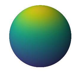
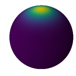
$\lambda=1,a=0$	$\lambda=10,a=0$
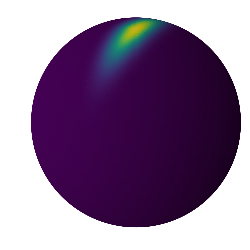
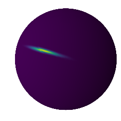
$\lambda=10,a=10$	$\lambda=25,a=100$, rotated

Figure 3. Visualization of NASG compoent $G$ with different parameters. Note that $G$ agrees with sperical Gaussian when $a=0$.

NASG satisfies all requirements as a model for learning the distribution for unbiased rendering. Different from ASG (Xu et al., 2013), NASG has an analytical closed form solution for its integral (see Appendix B), which makes it easy to normalize:

(9) $$K=\int_{S^{2}}G(\bm{\mathbf{v}};[\bm{x,y,z}],\lambda,a)d\omega=\frac{2\pi\left(1-e^{-2\lambda}\right)}{\lambda\sqrt{1+a}}.$$

NASG is also expressive as it can model anisotropic distributions, as well as high and low frequency distributions . It is also compact as it is parameterized by only 7 scalars, making it highly efficient in GPU-based computation due to its low bandwidth requirement. Additionally, the sampling algorithm of NASG is remarkably efficient (see Appendix C). These characteristics make NASG a highly feasible and practical option for our framework.

5. Online learning of Density Model

We now describe about our neural network structure for learning the parameters of our NASG model, as well as the training scheme.

5.1. Network Architecture

We wish our neural network to be as simple as possible considering the performance requirement for practical use. In this work, we use a 4-layer MLP, where each layer has 128 units without bias.

Network Inputs

The input to the model consists of the location of the shading point $\mathbf{x}$, the outgoing ray direction $\omega_{o}$ and surface normal $\mathbf{n}$. The location of the shading point is first encoded into a 57 dimention vector by positional encoding. Thus, the input size is 63 (57 + 3 + 3), but is padded to 64 for hardware acceleration purpose. We adopt the simple one-blob’encoding (Müller et al., 2019), instead of other complex encoding mechanics such as (Müller et al., 2022), as there was improvement in our pilot study versus the overhead they introduce. Details of the encoding scheme can be found in Table 1.

Table 1. Encoding scheme

Parameter	Symbol	Encoding
Position	$p\in{\mathbb{R}^{3}}$	$ob(p)$
Outgoing ray direction	$\omega_{o}\in{[-1,1]^{3}}$	$\omega_{o}$
Surface normal	$\mathbf{n}\in{[-1,1]^{3}}$	$\mathbf{n}$

Parameterization of NASG

To improve the efficiency of learning, we reduce the number of parameters for representing the NASG model. First, we introduce $\theta,\phi,\psi$, the Euler angles representing the orientation of the orthogonal basis with respect to the global axes. As such, $\bm{z}$ and $\bm{x}$ of the orthogonal basis can be represented by

(10) $$\bm{z}=\begin{pmatrix}\sin\theta\cos\phi\\ \sin\theta\sin\phi\\ \cos\theta\end{pmatrix},\ \bm{x}=\begin{pmatrix}\cos\theta\cos\phi\cos\psi-\sin\phi\sin\psi\\ \cos\theta\sin\phi\cos\psi+\cos\phi\sin\psi\\ -\sin\theta\cos\psi\end{pmatrix}.$$

Thus, we represent NASG with the following seven parameters: $\cos\theta$, $\sin\phi$, $\cos\phi$, $\sin\psi$, $\cos\psi$, $\lambda$, $a$.

Network Outputs

The output of our neural network is a $d$ dimensional vector $\bm{o}$, where each component corresponds to the NASG parameter at the shading point $\bm{\mathbf{x}}$ and a selection probability $c$. Assuming the number of mixture components is $N$, $d=5\times N+2\times N+N+1=8N+1$ (see Table 2). These parameters are further decoded to represent the actual parameters as summarized in Table 2.

Table 2. Decoding scheme for NASG with N components

Parameter	Symbol	Decoding
$\cos\theta$, $\sin\phi$, $\cos\phi$, $\sin\psi$, $\cos\psi$	$s_{0}\in{\mathbb{R}^{5\times N}}$	$\operatorname{sigmoid}(s_{0})\times 2-1$
$\lambda,a$	$s_{1}\in{\mathbb{R}^{2\times N}}$	$e^{s_{1}}$
Component weights	$\mathbf{A}\in{\mathbb{R}^{N}}$	$\operatorname{Tsm}(\mathbf{A})$
Selection probability	$c\in{\mathbb{R}}$	$\operatorname{sigmoid}(c)$

The mixture weights of NASG, $\mathbf{A}$, are normalized with second order Taylor softmax (Vincent et al., 2015) for computation stability, considering we usually calculate them in GPU with half-precision floating point numbers and “fast math mode” approximations:

(11) $$\operatorname{Tsm}(z)_{i}=\frac{1+z_{i}+0.5z^{2}_{i}}{\sum_{j=1}^{K}(1+z_{j}+0.5z^{2}_{j})}$$

5.2. Training

We now describe about our loss function and the training process. As shown in Fig. 4, we utilize automatic differentiation to train the network effectively with sparse online rendering samples. Since the training data are noisy online samples, we need a loss function that is more robust than regular L1 or L2 losses.

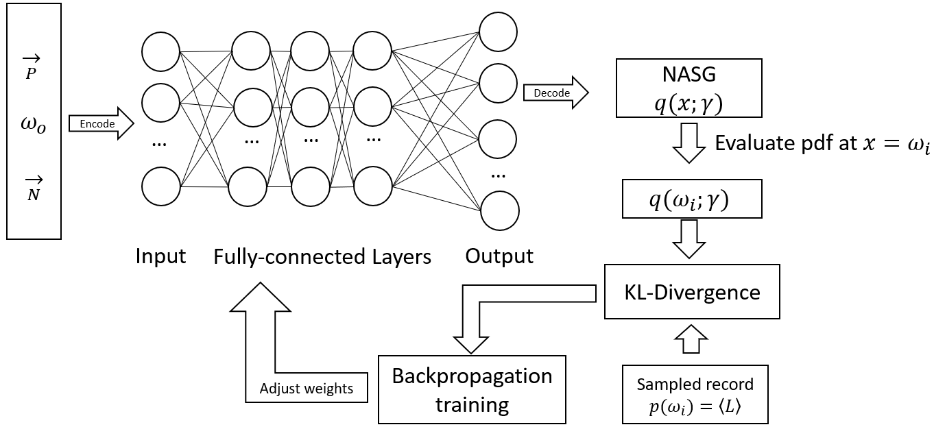
Figure 4. The training process of our network. We heavily utilize automatic differentiation to adjust weights of network based on estimated distribution and rendering estimation $\left<L\right>$ from sampled scattering direction $\omega_{i}$.

Kullback-Leibler Divergence

The design of a loss function for density distribution in PBR context is studied in several previous works including (Müller et al., 2019, 2020; Zhu et al., 2021b, a). Denoting $q(\omega_{i};\gamma)$ the NASG distribution (with NASG parameters $\gamma$) estimated by neural network, to achieve importance sampling of rendering equation, the optimal density distribution should be proportional to the product:

(12) $$q(\omega_{i};\gamma)\propto f_{s}(\mathbf{x},\omega_{i},\omega_{o})L_{i}|\cos\theta|.$$

Therefore, we use $p(\omega_{i})=Ff_{s}(\mathbf{x},\omega_{i},\omega_{o})L_{i}|\cos\theta|$ as our target distribution where $F$ is a normalizing term whose value is unknown. We can still train the system without knowing $F$ as we show below.

In our framework, we use the Kullback-Leibler Divergence (KL-Divergence) to represent the likelihood between our estimated density distribution $q(\omega_{i};\gamma)$ and the target one:

(13) $$D_{KL}(p(\omega_{i})||q(\omega_{i};\gamma))=\int_{\Omega}p(\omega_{i})(\log[p(\omega_{i})]-\log[q(\omega_{i};\gamma)])d\omega_{i}.$$

Since $p(\omega_{i})$ is $\gamma$-independent, we get

(14) $$\nabla_{\gamma}D_{KL}(p(\omega_{i})||q(\omega_{i};\gamma))=-\int_{\Omega}p(\omega_{i})\nabla_{\gamma}\log[q(\omega_{i};\gamma)]d\omega_{i}.$$

The integral can be replaced with our one-sample estimation:

(15) $$\nabla_{\gamma}D_{KL}(p(\omega_{i})||q(\omega_{i};\gamma))=-\,\mathbb{E}\left[\frac{p(\omega_{i})}{\hat{q}(\omega_{i};\gamma)}\nabla_{\gamma}\log[q(\omega_{i};\gamma)]\right],$$

where $\hat{q}(\omega_{i};\gamma)$ denotes the PDF of the distribution the sample obeys during rendering; see below. Though the right-hand side still involves the global scaling factor $F$, it will be canceled in moment-based optimizers such as Adam (Kingma and Ba, 2014); thus we can train the system even there is an unknown scaling factor in $p(\omega_{i})$ (Müller et al., 2019).

Selection Probability

Following (Müller et al., 2020), we do not directly use a distribution estimated by our neural network. Instead, we consider that our scattering sampling process is an MIS process that blends the learned distribution and the BSDF distribution $p_{f_{s}}(\omega_{i})$. As we also learn a selection probability $c$ as described in § 5.1, the MIS PDF at shading point $\bm{\mathbf{x}}$ is $\hat{q}(\omega_{i};\gamma)=cq(\omega_{i};\gamma)+(1-c)p_{f_{s}}(\omega_{i})$. However, optimizing $\hat{q}(\omega_{i};\gamma)$ naively will lead to falling into a local optima with degenerate selection probability; therefore our final loss function blends $\hat{q}(\omega_{i};\gamma)$ with $q(\omega_{i};\gamma)$:

(16) $$loss=eD_{KL}(p(\omega_{i})||\hat{q}(\omega_{i};\gamma))+(1-e)D_{KL}(p(\omega_{i})||q(\omega_{i};\gamma))$$

where $e$ is a fixed fraction which we set to 0.2.

6. Implementation Details

We integrate our framework to an in-house GPU wavefront path tracer. In this section we discuss about implementation details as well as design considerations.

Progressive Learning and Sampling

Our framework collects samples to train the network online, and use the network to generate a distribution, which is then blended with the BSDF sampling distribution using the learned selection probability $c$. We further multiply an extra coefficient $b$ to compute an actual blending weight $c^{\prime}=bc$, where $b$ is initially set 0 and gradually increased to 1, such that the framework initially relies on BSDF distribution, and gradually switches to the learned distribution $\hat{q}(\omega_{i};\gamma)$. We use a fixed-step strategy to ensure our guided sampling uses enough number of samples for learning the distribution: for every $M$ images rendered, we increase $b$ by $\frac{1}{R}$. In our implementation, we set $M=4$ and $R=64$. This could require adjustments according to rendering task, further discussions are given in § 8.2.

For rendering images while progressively learning the distribution, previous works (Müller et al., 2017, 2019, 2020) blend the rendered image samples based on their inverse variance. Such a process will introduce extra memory and computation overhead, especially for a renderer that produces arbitrary output variables (AOVs). Based on the observation that variance of individual image pixel decreases as the learning proceeds, we use a simplified method which scales the weights of accumulated results according to the training steps. This essentially gives more weight to later samples in a progressive manner, and the result is still unbiased. The weight scaling process stops when the training step count reaches $M\times R$.

CPU-based Network Optimization

The process of distribution learning runs on CPU in parallel to the main rendering task being executed on GPU. We use Pytorch (Paszke et al., 2017) for the implementation, along with Adam optimizer whose learning rate is set to 0.02. When rendering image, we split the image into smaller tiles, whose size is set to $l\times l$, and collect data from one pixel per tile in each render iteration. We set the maximum size of training samples in each iteration to $S=2^{14}$. If the number of training samples reaches $S$ in the middle of the iteration, $l$ is increased by one in the next iteration. If the number of samples is less than $S/2$ at the end of iteration, $l$ is decreased by one. The collected data are sent to the CPU after each render iteration for progressively training the model.

Direct Lighting with NEE

Our implementation uses MIS to blend guided scattering directions with Next Event Estimation (NEE) to sample direct lighting. NEE helps to improve the quality of the images especially in the beginning of the training stage. It is to be noted that MIS is only possible because our model is an explicit model that allows us to freely sample the distribution and evaluate PDF at certain direction; which could be difficult for methods such as  (Müller et al., 2019, 2020). Our MIS strategy also helps to improve the the sampling efficiency for effects where direct light plays a key role (e.g., soft shadows).

Wavefront Architecture

Neural network computation can be greatly accelerated with hardware (e.g., Tensor Core). However, such hardware is usually designed for batched execution, in which a single matrix multiplication involves multiple threads. This conflicts with the classic thread-independent “Mega-kernel” path tracing implementation. Our implementation adopts “Wavefront path tracing” architecture (Laine et al., 2013) to solve this problem. In a wavefront path tracer, all the pixels at the same stage will be executed concurrently. With this condition, we are able to “insert” our neural network calculation seamlessly right before the sampling/shading stage, and minimize the computation overhead for best performance. The forward pass of our MLP does not require gradient calculation, therefore we implement it on GPU with CUBLAS, and the result implementation is substantially faster than using existing deep learning framework.

7. Results

We render a variety of scenes with our framework and compare the results with those rendered by two other methods: classic path tracing (with NEE) and a GPU implementation of Practical Path Guiding (PPG). Our PPG implementation is based on (Müller, 2019) and the authors’ CPU implementation, while different from the authors’ version in two aspects: (1) we use voxels instead of octree for spatial data structure for efficient GPU-based refinement, and (2) NEE is considered for improving the quality of the rendered images. We do not compare our result with off-line methods or normalizing-flow-based online methods, because of the unmatched requirement of computation resource. More sophisticated online learning methods (e.g., (Dodik et al., 2022; Rath et al., 2020)) are not compared due to the difficulty of implementation to a GPU path tracer. In the following experiments, we run our path tracer with a conventional PC with a 4-core i7 9700K CPU and an NVIDIA 2080ti GPU. The implementation of our framework introduces roughly 600 MB memory overhead on GPU, mainly for buffer of batched network execution. All the images are also included in the supplemental material. We use mean absolute percentage error (MAPE) as the metric.

7.1. Variance Reduction

Fig. 5 shows a same-sample comparison of different methods. Every image is rendered with 1024 samples per pixel (spp). “Veach Bidir” scene demonstrates basic application of our framework in regular 3D scenes that consist of many complex light paths that are difficult to be sampled with unidirectional path tracing. “Light Cage” is a typical difficult scene where only emissive geometry is used to light the space and it requires capability to learn high frequency varying distributions. “Kitchen 1” scene is a more complex scene where the refracted lighting on the floor is the major illumination. The result shows both robustness and efficiency of our method. Our framework achieves lowest variance in all scenes. PPG performs generally well in scenes where indirect lighting is dominant, however, due to its partition-based learning, it shows limitation on learning high-frequency spatial varying distribution and gives higher variance for the “Light Cage” scene. We also find in scenes where sampling can greatly benefit from NEE (the “Ajar” scene for example), the variance of PPG is slightly higher than unidirectional path tracing, which is consistent with experiment results in previous work (e.g., (Zhu et al., 2021b)).

		PT	NPG (Ours)	PPG	Reference
VEACH BIDIR
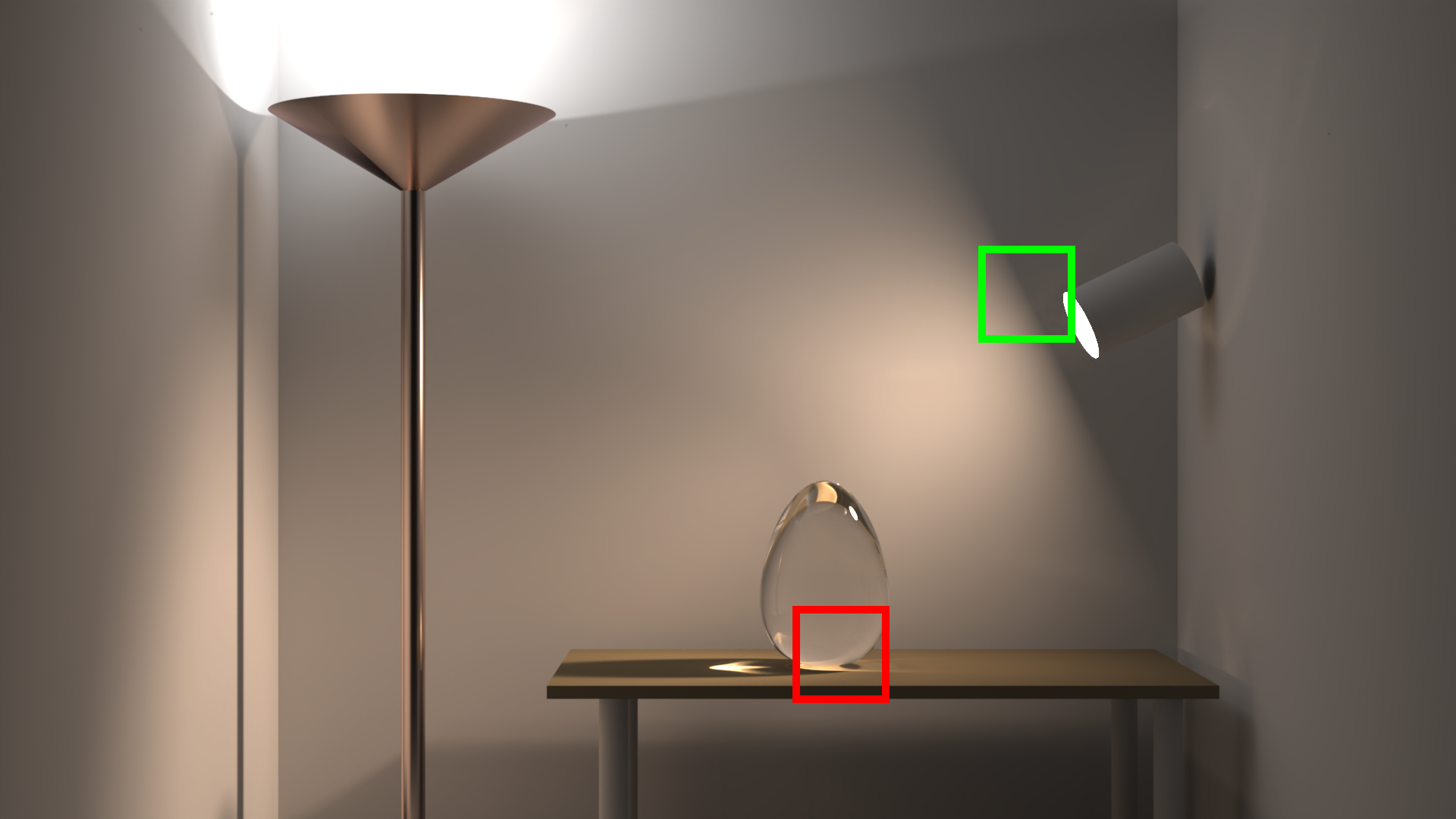
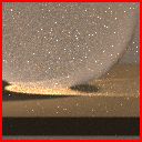
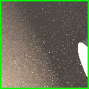
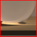
	MAPE:	0.253	0.078	0.078
LIGHT CAGE
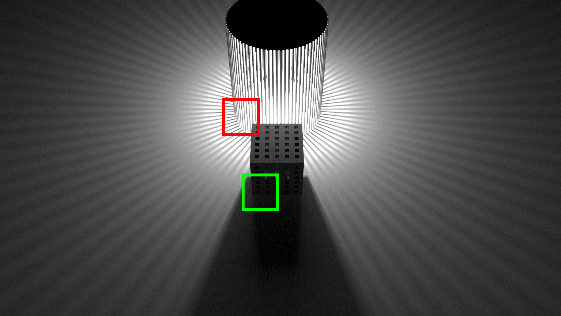
	MAPE:	1.34	0.220	0.395
KITCHEN 1
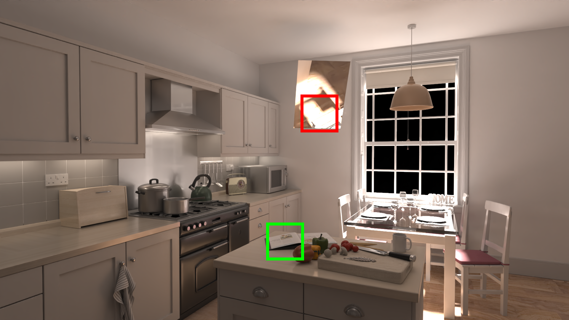
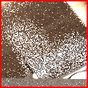
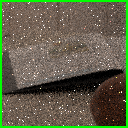
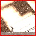
	MAPE:	0.617	0.062	0.462
AJAR
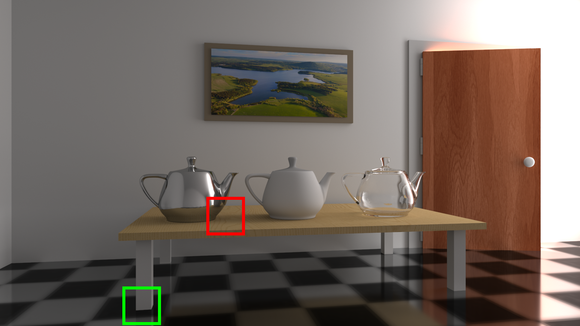
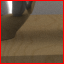
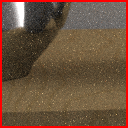
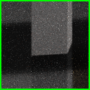
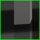
	MAPE:	0.147	0.051	0.136

Figure 5. Rendering result of different methods under same 1024 sample-per-pixel (SPP). All images are $1920\times 1080$ pixels. The mean absolute percentage error (MAPE) indicates that our method (NPG) outperforms plain path tracing (PT) and (Müller, 2019) (PPG) in all scenes. PPG achieves low variance in scenes where narrow indirect lighting is dominant (“Veach Bidir”, “Light Cage”, and “Kitchen 1”), however in scenes with more general lighting setup (“Ajar”) it fails to outperform unidirectional path tracing with NEE.

7.2. Equal Time Comparison

As a performance-centered framework, we also conduct equal time comparison to intuitively evaluate raw performance of our framework compared to PPG and classic path tracing. For every scene, we perform 5-minute rendering including any extra learning computation on the same hardware. With careful implementation, our framework has a low overhead than previous neural-network-based frameworks such as (Müller et al., 2020; Zhu et al., 2021a). As shown in Fig. 6, our framework achieves a general boost of sampling efficiency compared to a plain path tracer in every test scene. Given the same time budget our framework achieves lowest variance in all test scenes, including “Kitchen 2” which is mainly lit by a large area light, and considered as an example which benefits little from guiding.

		PT	NPG (Ours)	PPG	Reference
CORRIDOR
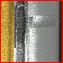
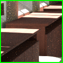
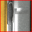
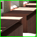
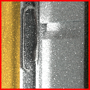
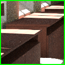
	MAPE:	0.174	0.096	0.150
	SPP:	4855	1887	2031
POOL
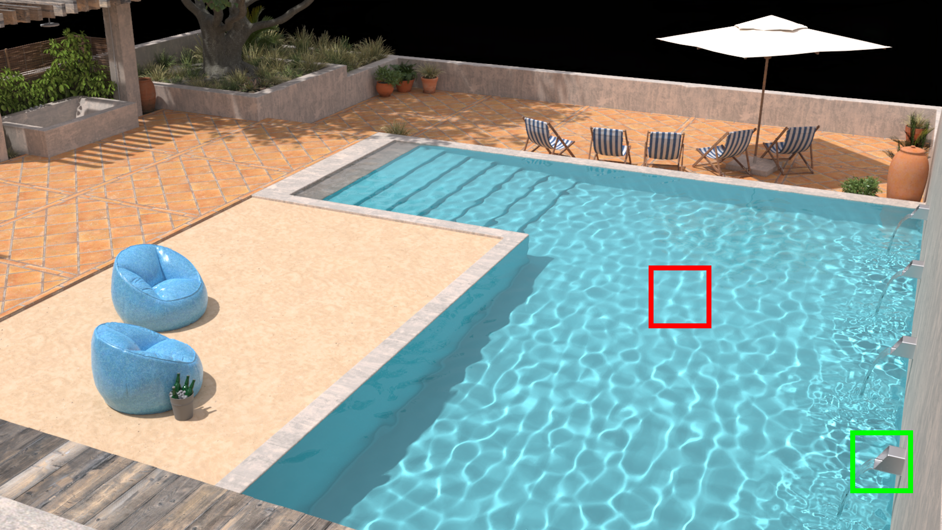
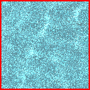
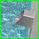
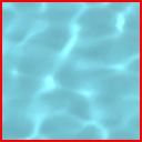
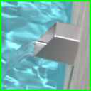
	MAPE:	0.298	0.046	0.149
	SPP:	3772	1521	1764
KITCHEN 2
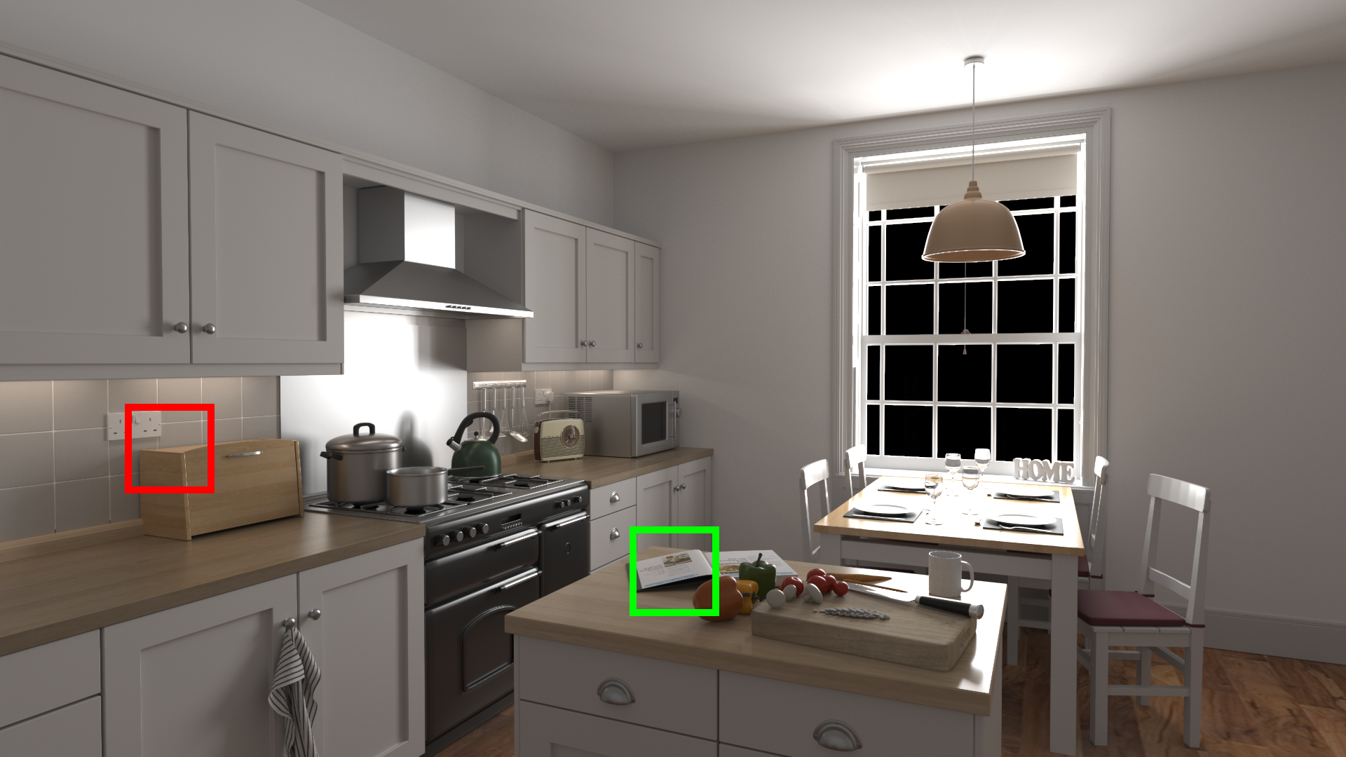
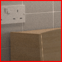
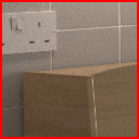
	MAPE:	0.042	0.041	0.101
	SPP:	3402	1386	1433
BATHROOM
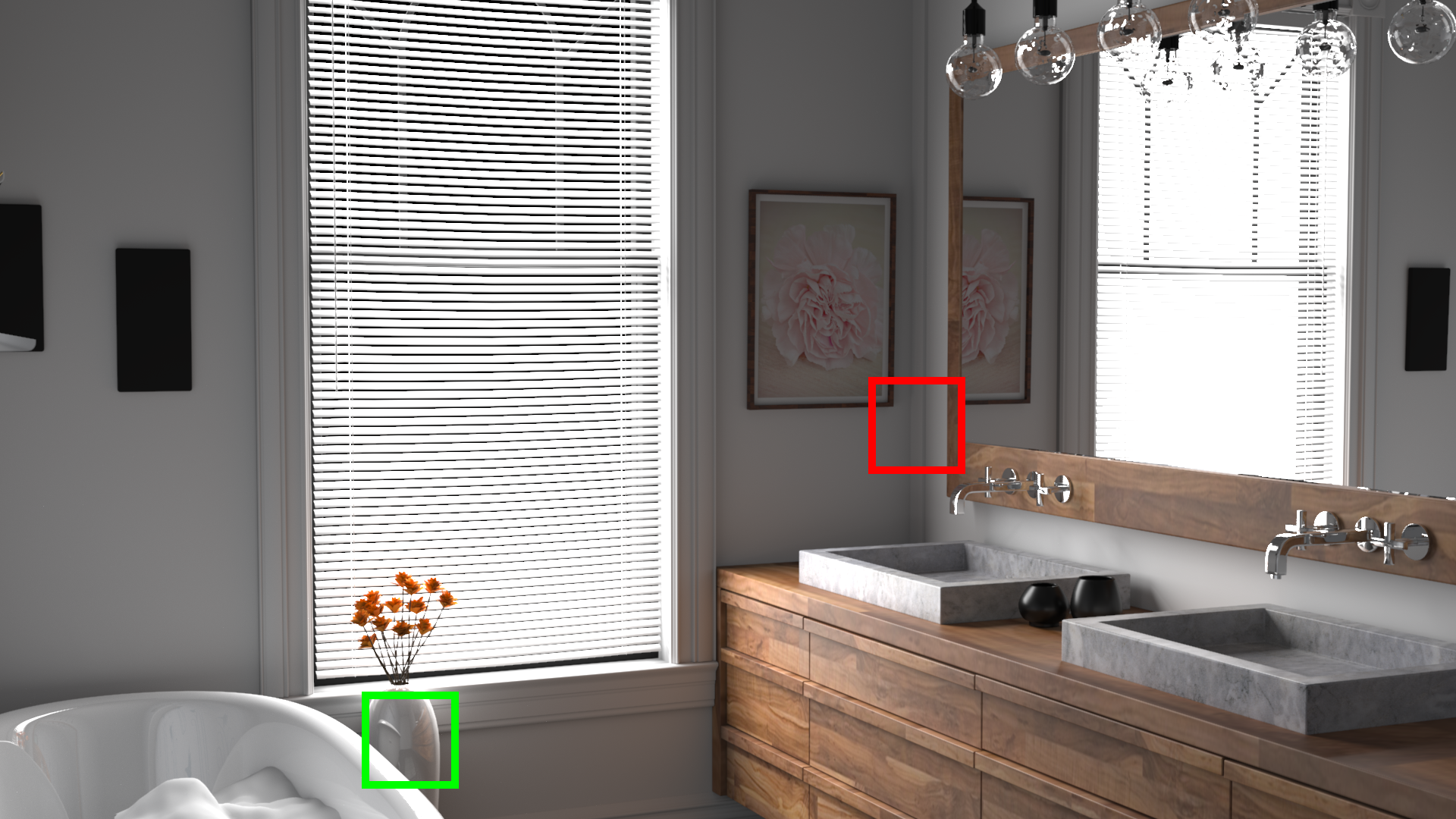
	MAPE:	0.081	0.063	0.110
	SPP:	3735	1456	1611

Figure 6. Equal time comparison. We render all the images for 5 minutes and compare the error measured in MAPE. The tolal SPP is also recorded. Our framework introduces an  150% overhead on top of plain path tracing (mostly due to neural network execution and additional memory traffic), however since the sampling efficiency is greatly improved, the results still surpass PT and PPG.

7.3. Density Models and Meta-parameters

In this section, we compare the expressiveness of NASG with other density models including (Gilboa et al., 2021)(MDMA), SG (Wang et al., 2009), and bivariate Gaussian (Vorba et al., 2014). For the other models, the network outputs their parameters in a fashion similar to the setup for NASG.

We limit the number of parameters to 256 for all models for a fair comparison. As shown in Fig. 7, in all the test scenes our NASG gives lowest MAPE. We also notice that results of bivariate Gaussian (G2D) contains more outliers, this is due to the domain mismatch problem mentioned in § 2.4.

		MDMA	SG	G2D	NASG
KITCHEN 2
	MAPE:	0.077	0.069	0.109	0.065
CORRIDOR
	MAPE:	0.150	0.139	0.189	0.131

Figure 7. Rendered result with our framework adopting different normalized density models. All images are rendered with 5 minutes, and parameter number of different models are set to be 256. Our proposed NASG achieves lowest variance in both test scenes.

We also compare the results with different meta-parameters of the system. To best evaluate the results we perform equal-time rendering with different configurations. Fig. 8 shows the results produced with different number of hidden units and NASG components. Increasing hidden units results in higher variance; this is because computation of neural network is the major overhead for the whole framework and more hidden units significantly increases the computation time. While the improvement of accuracy is not affected much, the sample counts within the same computational time is reduced.

		HU=128, C=4	HU=128, C=8	HU=256, C=4	HU=256, C=8
BATHROOM
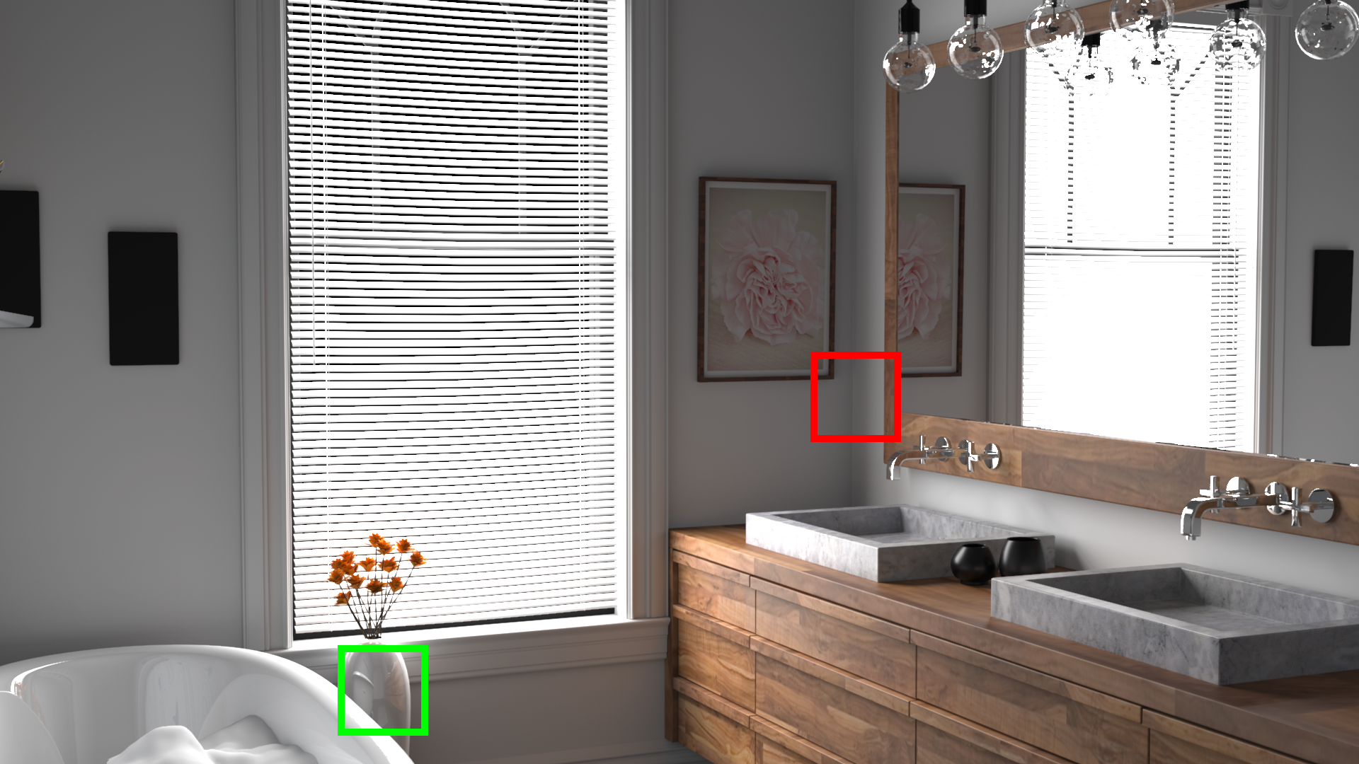
	MAPE:	0.057	0.058	0.064	0.065
AJAR
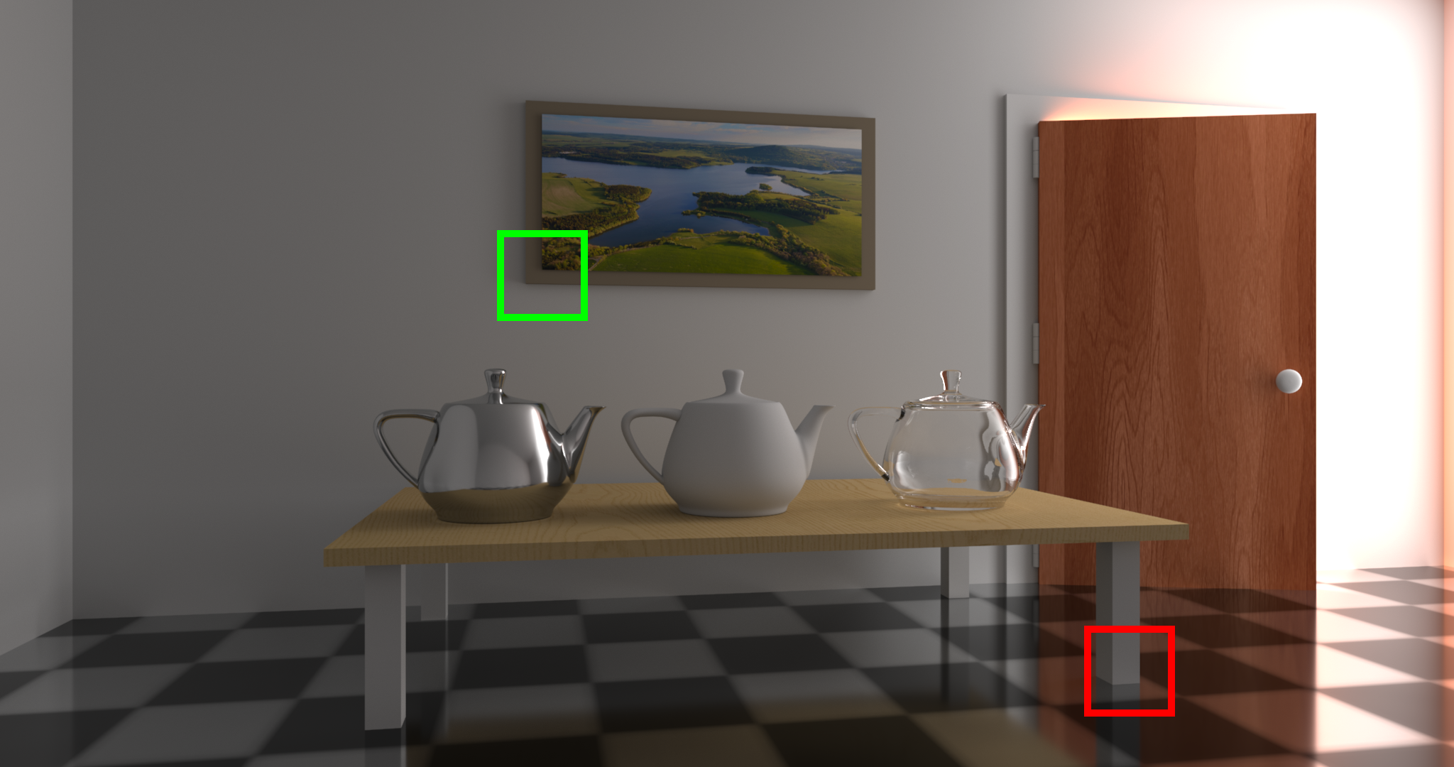
	MAPE:	0.055	0.056	0.067	0.069

Figure 8. We further evaluate the variance reduction of different parameter configurations of NASG. We use different number of hidden units(HU) and components (C) and render scenes with equal time. All results show similar variance, however the simplest configuration with HU=128 and C=4 achieves  20% lower MAPE than most complex configuration with HU=256 and C=8. This shows that all configurations can learn distribution well, however complex configuration has higher overhead hence lower raw performance.

In terms of NASG, we find that the 4-component setup has only minor difference compared to the 8-component setup. This is because for most situations, the 4-component NASG is expressive enough to learn the distribution.

7.4. Learned Components

Our framework learns distribution and selection probability with single neural network. In Fig. 9 we visualize examples of the learned components in two actual rendering scenes. Our learned selection probability tends to rely more on our learned distribution where surface is rough, while smooth surface and where direct lighting is dominant prefers BSDF distribution. The learned contribution fits the reference closely and the high energy spots are accurately localized. Our framework is able to closely fit high-frequency narrow distributions with NASG. PPG fails to learn a good distribution for yellow point of the “Box” scene, even we use a high-resolution voxel structure for caching. This is a known limitation when the light distribution within the corresponding cache cell drastically varies (since the light source is very close to the red wall, a small difference in position leads to large difference in direction of incoming light). In contrast, our framework can learn such spatial-varying distribution accurately with proper position encoding scheme.

	CORRIDOR	BOX
Reference
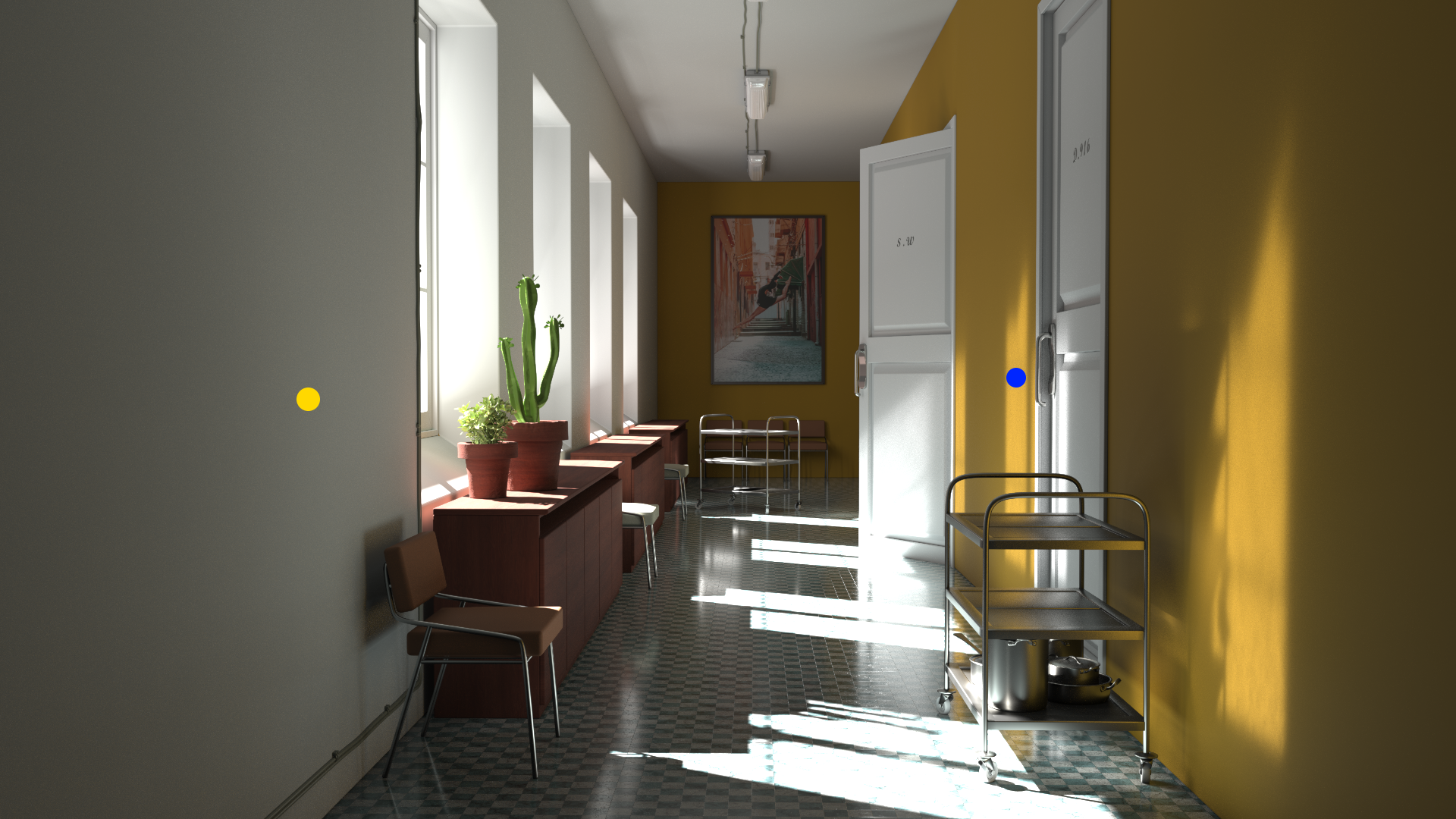
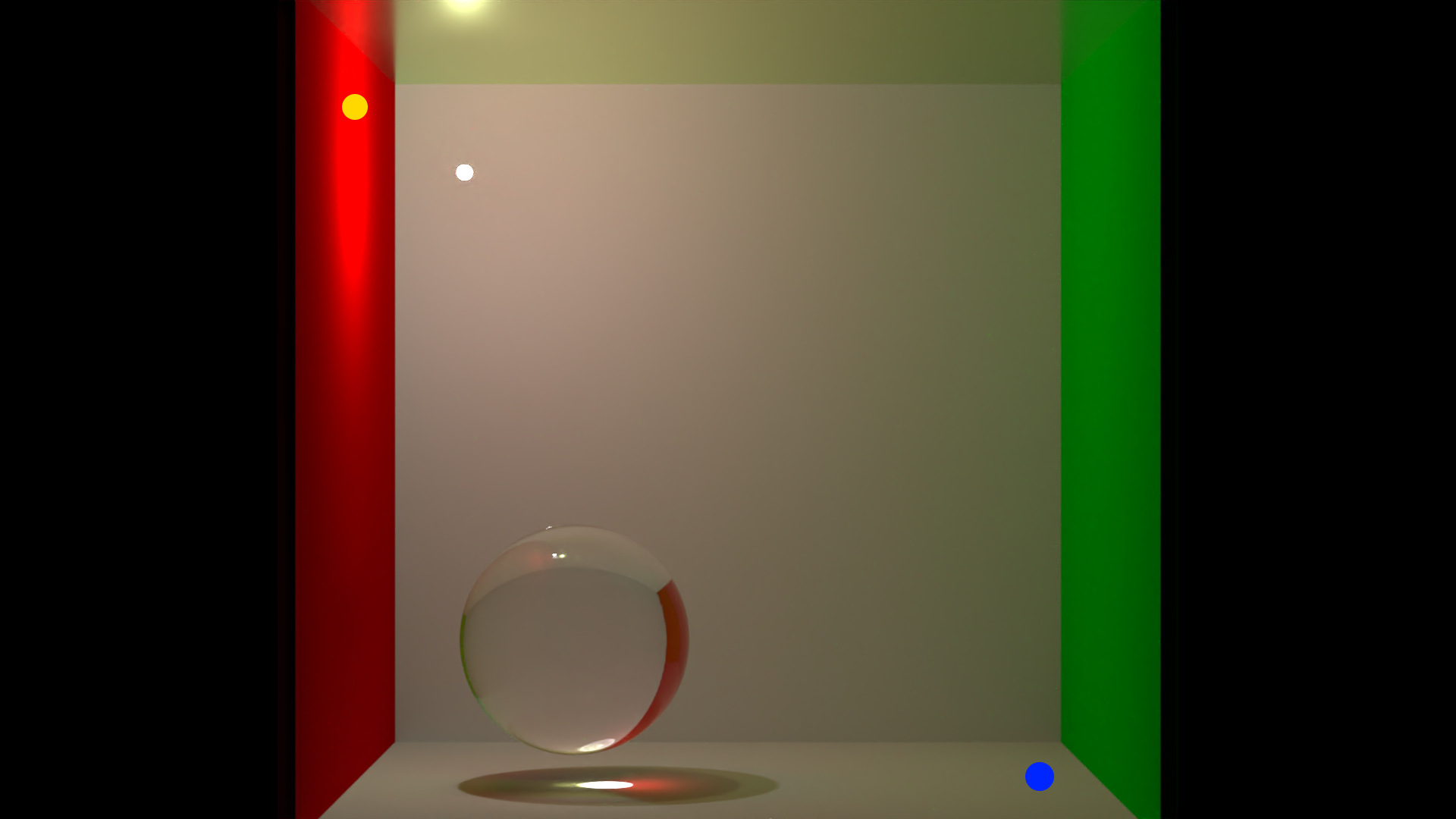
Selection Probability
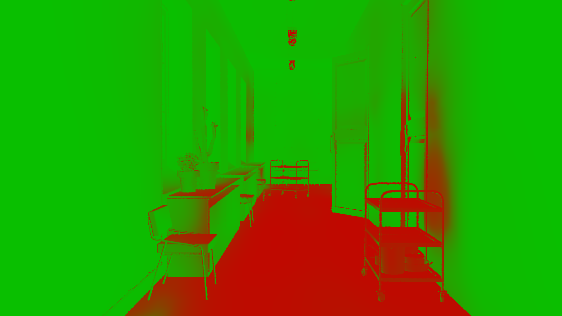
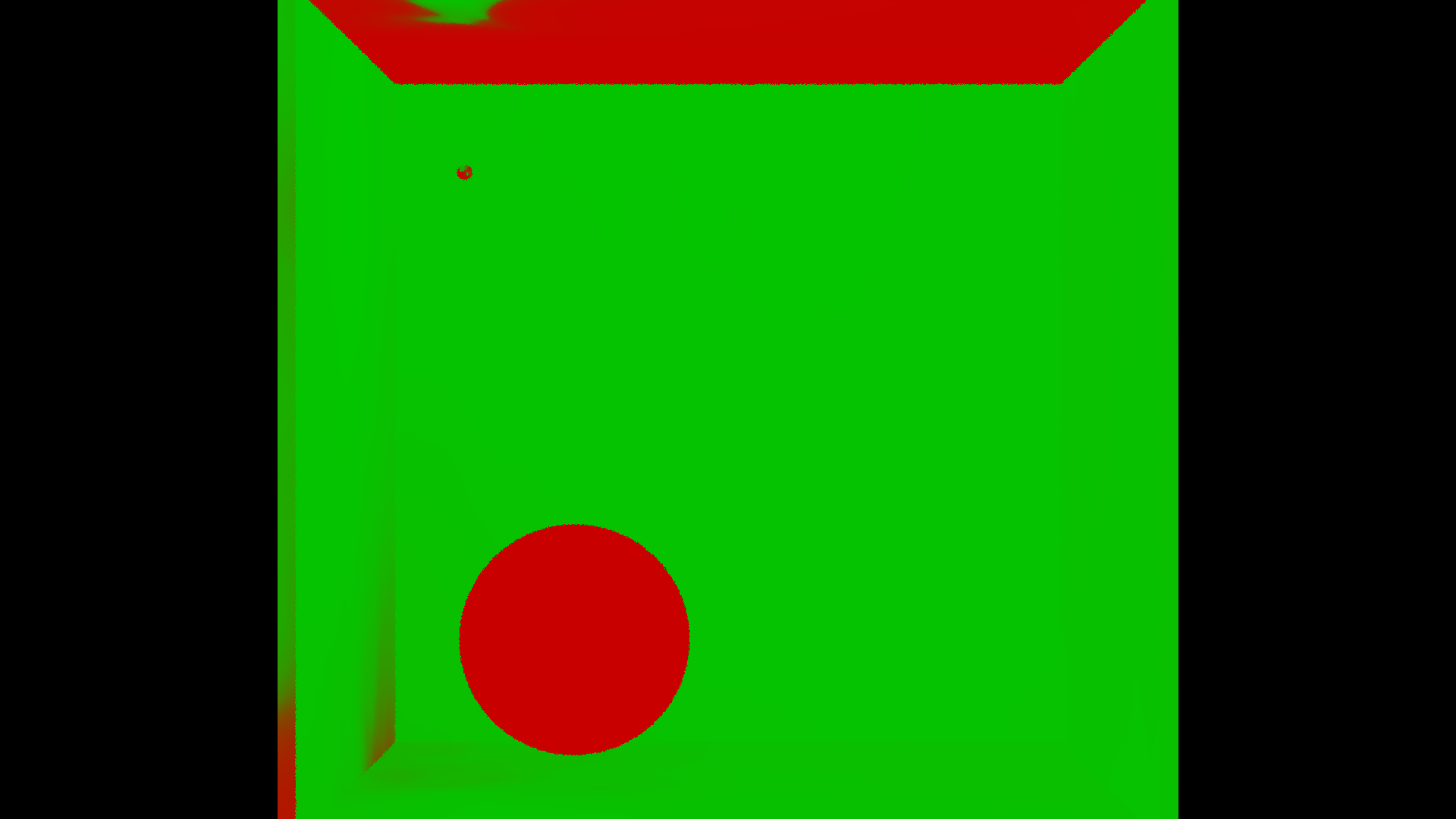
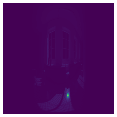
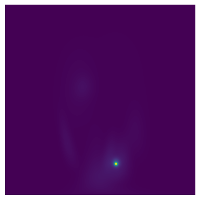
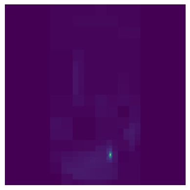
Blue	Reference Ours PPG	Reference Ours PPG
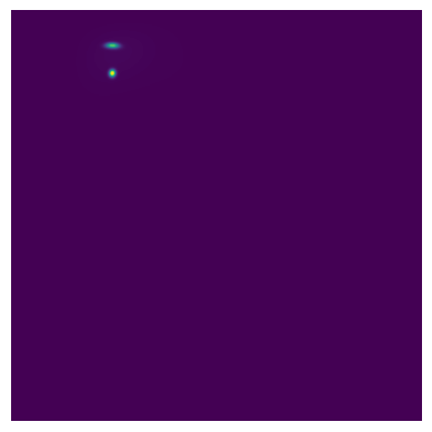
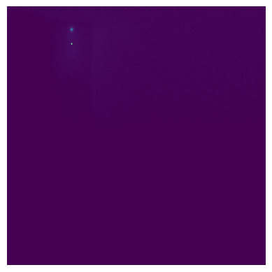
Yellow

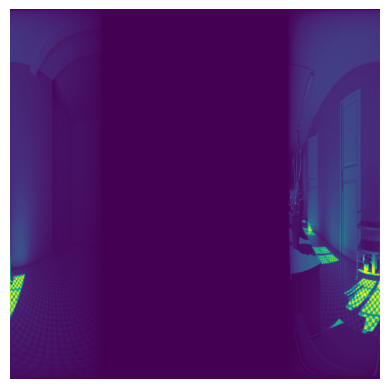
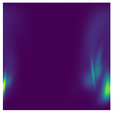
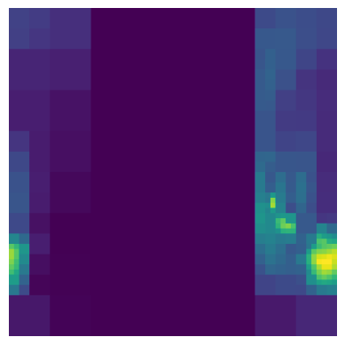
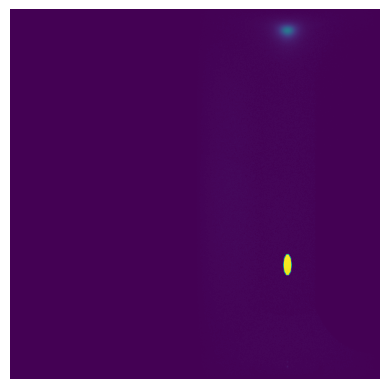
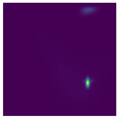
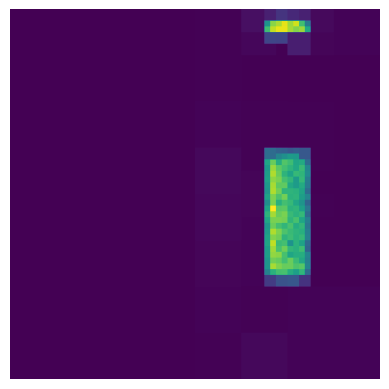
Figure 9. Visualization of learned selection probability and distribution. Our framework uses a single neural network to learn these two components accurately. The selection probability determines the blending weight of two distributions we can sample from: our learned product distribution (green) and BSDF distribution of surface (red). Smooth surface prefers BSDF distribution while rough one prefers learned product distribution. Our result is consistent with previous works such as (Müller et al., 2020) which learns selection probability and lighting distribution separately. “Blue” and “Yellow” show distribution obtained with both our framework and PPG, in compare with the reference. Readers are encouraged to zoom in to view the details.

7.5. Guided Direct Lighting

As shown in Fig. 10, we render direct lighting of a simple scene with certain occlusion, blending NEE with both BSDF distribution and our learned distribution, for 1024 samples. The variance of our learned distribution result is slightly lower than BSDF distribution, and soft shadow appears to be less “noisy”. The result shows that both direct and indirect lighting can benefit from our framework.

	Guided	Unidirectional	Reference
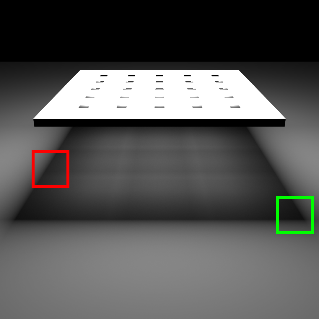
MAPE:	0.050	0.058

Figure 10. Rendering result of direct lighting using NEE, blending with guided and unidirectional scattering samples. Both results are rendered with 512 samples-per-pixel (SPP). Our guided result has lower variance, and the soft shadows appear to be less noisy.

7.6. Weight Reuse

When rendering in a (relatively) static scene with moving cameras, reusing weights of neural network rather than initializing them every frame can further reduce variance. This is because our model learns the spatial-varying density distribution for the whole sampled space. Fig. 11 shows an example of rendering with weight reuse, and readers are referred to supplementary video for a comparison of weight reuse in a full sequence of the corresponding fly-through cut.

	Reused	From scratch	Reference
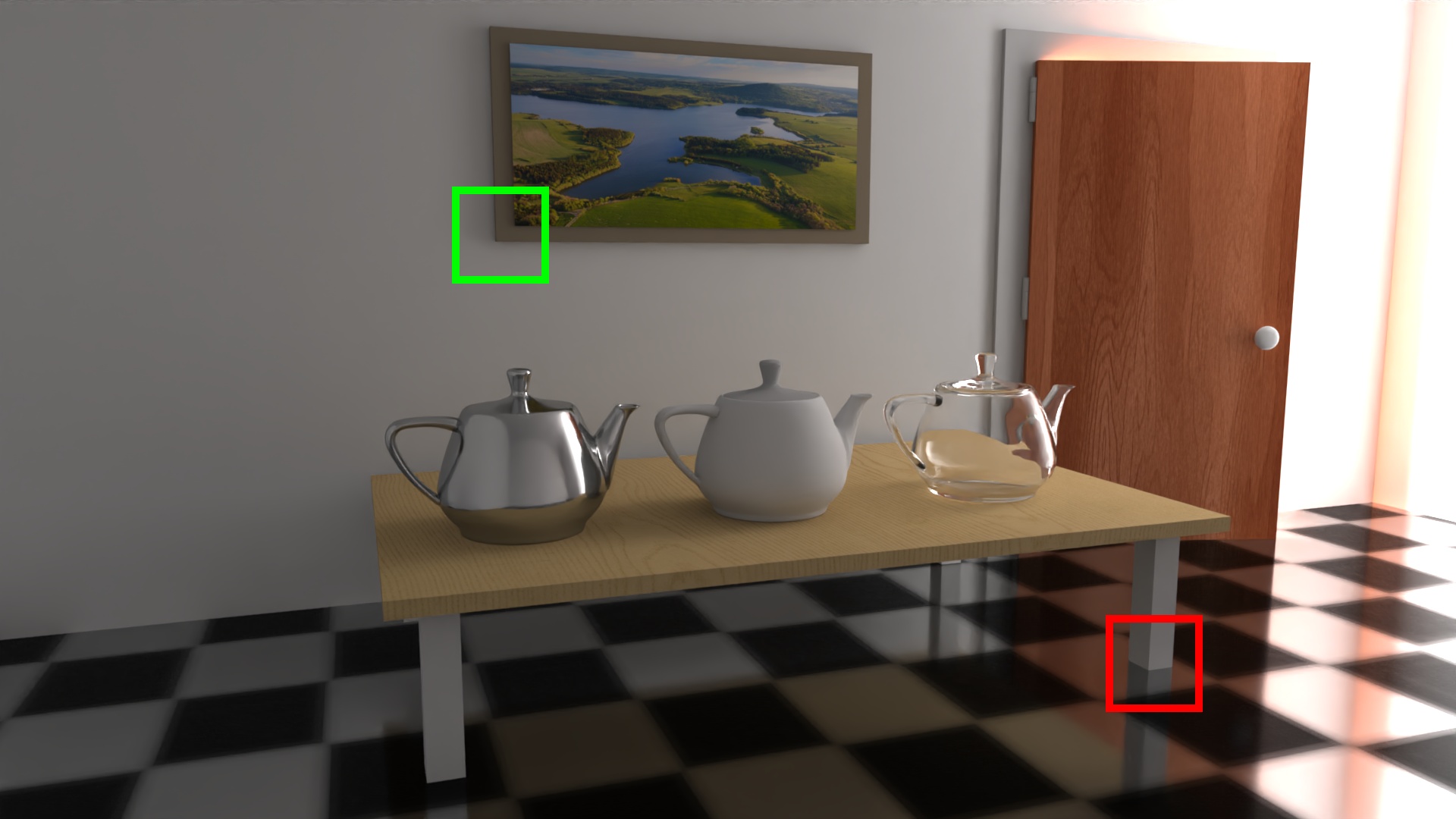
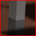
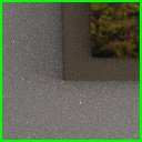
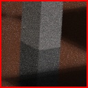
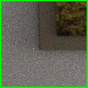
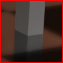
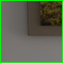
MAPE:	0.104	0.127

Figure 11. Rendering result with/ without weight reuse. The image is a frame in the middle of a fly-through cut. With weight reuse, we take the weights from previous frame as the initial weights to start rendering and continue optimizing the neural network. Weight reuse helps to further reduce variance in rendering of (relatively) static scene with novel views.

8. Discussion

8.1. Performance in GPU Path Tracing

A GPU-based brute-force path tracer could be 20x faster than a CPU-based one. If an importance sampling method provides low per-sample variance yet with high overhead, it can not beat a brute-force path tracer on GPU. To this end, we eliminate normalizing-flow-based methods since the computational overhead is not acceptable in our application scenario. Besides powerful computation ability, GPU has limited memory bandwidth and size, and memory latency is much more obvious than CPU memory, causing many CPU algorithms to perform relatively slow in GPU (e.g., PPG’s quad-tree representation requires random access to GPU memory for multiple times, which causes long stall on GPU due to memory latency).

8.2. Limitation and Future Work

During experiment we found that parameters of learning strategy we mentioned in § 6 needs to be carefully chosen among different rendering tasks. Although in general we can use a very aggressive configuration and it works well, we encountered several cases where we need to have bigger $M$ to avoid degenerate distribution. This usually happens in rendering of caustics. Our explanation is when the distribution is difficult to be learned (e.g., due to poor sampling efficiency), using the learned distribution too soon will lead to even worse samples, and the learning result could never recover from degeneration. It is worth trying to propose an adaptive configuration of learning strategy to improve the robustness of our framework and we leave it as a future work.

The most interesting extension of our framework would be guiding with participating media. This could be achieved in theory (similar approach to (Herholz et al., 2019)), yet further the ability to learn 3D distribution remains to be investigated.

9. Conclusion

In this paper we propose an effective online neural path guiding framework for unbiased physically-based rendering. We tackle the major challenges of neural-based online path guiding methods by proposing a novel closed-form density model, NASG. The simplicity and expressiveness of NASG allow it to be efficiently learned online via a tiny, MLP-based neural network. We also propose the online training strategy to train a neural network with sparse ray samples.

Our framework helps to improve the raw performance of path tracer via neural path guiding. Under the same computational time constraint, our framework outperforms state-of-the-art path guiding techniques. This is because our framework can effectively learn the spatial-varying distribution and guide a unidirectional path tracer with low overhead, allowing a path tracer to produce high quality images with limited computational resources. Our work also shows that learning-based importance sampling has a great potential in practical rendering tasks. We hope our work can help pave the path for the research communities in industries and academia for adopting neural technologies for path tracing.

Appendix A Continuity of NASG

The complete form of a NASG component is given by:

(17) $$G(\bm{\mathbf{v}};[\bm{x,y,z}],\lambda,a,\epsilon,\kappa)$$

$$\quad=\begin{cases}\kappa\cdot\exp\left(2\lambda\left(\frac{\bm{\mathbf{v}}\cdot\bm{z}+1}{2}\right)^{1+\epsilon+\frac{a(\bm{\mathbf{v}}\cdot\bm{x})^{2}}{1-\left(\bm{\mathbf{v}}\cdot\bm{z}\right)^{2}}}-2\lambda\right)\left(\frac{\bm{\mathbf{v}}\cdot\bm{z}+1}{2}\right)^{\epsilon+\frac{a(\bm{\mathbf{v}}\cdot\bm{x})^{2}}{1-(\bm{\mathbf{v}}\cdot\bm{z})^{2}}}\\ \hskip 147.95433pt\text{ if }\bm{\mathbf{v}}\cdot\bm{z}\neq\pm 1\\ \kappa&\text{ if }\bm{\mathbf{v}}\cdot\bm{z}=1\\ 0&\text{ if }\bm{\mathbf{v}}\cdot\bm{z}=-1\end{cases}$$

where $\kappa$ is the lobe amplitude and $\epsilon$ is an auxiliary parameter introduced so that $G$ is continuous whenever $\epsilon>0$. In practise, it is possible to set $\epsilon=0$, although this breaks continuity at $\bm{\mathbf{v}}=-\bm{z}$ unless $a=0$. For the rest of content we set $\kappa=1$ and omit it from the notation.

Appendix B Derivation of the normalizing term

Consider an NASG component defined as $G(\bm{\mathbf{v}};[\bm{x,y,z}],\lambda,a,\epsilon)$. Since $G$ is rotation invariant, we assume that $\bm{x}=(1,0,0)$, $\bm{y}=(0,1,0)$, and $\bm{z}=(0,0,1)$. Then the surface integral of the function $G$ over $S^{2}$ is given by:

(18) $$\int_{S^{2}}G(\bm{\mathbf{v}};[\bm{x,y,z}],\lambda,a,\epsilon)d\omega$$

$$=\int_{0}^{2\pi}d\phi\int_{0}^{\pi}\exp\left(2\lambda\left(\frac{\cos\theta+1}{2}\right)^{1+\epsilon+a\cos^{2}\phi}-2\lambda\right)$$

$$\hskip 113.81102pt\left(\frac{\cos\theta+1}{2}\right)^{\epsilon+a\cos^{2}\phi}\sin\theta d\theta.$$

We compute the inner integral over $\theta$ first. Consider the following change of variable (for fixed $\phi$):

(19) $$\frac{\cos\theta+1}{2}=\left(\frac{\cos\tau+1}{2}\right)^{\frac{1}{1+\epsilon+a\cos^{2}\phi}}$$

$$\Leftrightarrow \cos\theta=2\left(\frac{\cos\tau+1}{2}\right)^{\frac{1}{1+\epsilon+a\cos^{2}\phi}}-1.$$

where $0\leqslant\tau\leqslant\pi$. Then

(20) $$-\sin\theta d\theta=\frac{2}{1+\epsilon+a\cos^{2}\phi}\left(\frac{\cos\tau+1}{2}\right)^{\frac{1}{1+\epsilon+a\cos^{2}\phi}-1}\left(-\frac{\sin\tau}{2}\right)d\tau,$$

so

(21) $$\sin\theta d\theta=\frac{1}{1+\epsilon+a\cos^{2}\phi}\left(\frac{\cos\tau+1}{2}\right)^{-\frac{\epsilon+a\cos^{2}\phi}{1+\epsilon+a\cos^{2}\phi}}\sin\tau d\tau,$$

and the inner integral with respect to $\theta$ becomes:

(22) $$\frac{1}{1+\epsilon+a\cos^{2}\phi}\int_{0}^{\pi}\exp(\lambda\cos\tau-\lambda)\sin\tau d\tau$$

$$=\frac{1}{1+\epsilon+a\cos^{2}\phi}\left[-\frac{\exp(\lambda\cos\tau-\lambda)}{\lambda}\right]_{0}^{\pi}$$

$$=\frac{1-e^{-2\lambda}}{\lambda(1+\epsilon+a\cos^{2}\phi)}.$$

Hence it follows that

(23) $$\int_{S^{2}}G(\bm{\mathbf{v}};[\bm{x,y,z}],\lambda,a,\epsilon)d\omega$$

$$=\frac{1-e^{-2\lambda}}{\lambda}\int_{0}^{2\pi}\frac{d\phi}{1+\epsilon+a\cos^{2}\phi}$$

$$=\frac{2(1-e^{-2\lambda})}{\lambda}\int_{-\frac{\pi}{2}}^{\frac{\pi}{2}}\frac{d\phi}{1+\epsilon+a\cos^{2}\phi}.$$

Now, consider the following change of variable:

(24) $$\tan\phi=\sqrt{\frac{1+\epsilon+a}{1+\epsilon}}\tan\rho.$$

Then

(25) $$\frac{d\phi}{\cos^{2}\phi}=\sqrt{\frac{1+\epsilon+a}{1+\epsilon}}\frac{d\rho}{\cos^{2}\rho},$$

where

(26) $$\cos^{2}\phi =\frac{1}{1+\tan^{2}\phi}$$

$$=\frac{1}{1+\frac{1+\epsilon+a}{1+\epsilon}\tan^{2}\rho}$$

$$=\frac{1+\epsilon}{\frac{1+\epsilon+a}{\cos^{2}\rho}-a}$$

$$=\frac{(1+\epsilon)\cos^{2}\rho}{1+\epsilon+a-a\cos^{2}\rho},$$

so

(27) $$d\phi=\frac{\sqrt{(1+\epsilon)(1+\epsilon+a)}}{1+\epsilon+a-a\cos^{2}\rho}d\rho.$$

Hence it follows that

(28) $$\int_{S^{2}}G(\bm{v};[\bm{x,y,z}],\lambda,a,\epsilon)d\omega$$

$$=\frac{2(1-e^{-2\lambda})}{\lambda}\int_{-\frac{\pi}{2}}^{\frac{\pi}{2}}\frac{1}{1+\epsilon+\frac{(1+\epsilon)a\cos^{2}\rho}{1+\epsilon+a-a\cos^{2}\rho}}\cdot\frac{\sqrt{(1+\epsilon)(1+\epsilon+a)}}{1+\epsilon+a-a\cos^{2}\rho}d\rho$$

$$=\frac{2(1-e^{-2\lambda})}{\lambda}\int_{-\frac{\pi}{2}}^{\frac{\pi}{2}}\frac{d\rho}{\sqrt{(1+\epsilon)(1+\epsilon+a)}}$$

$$=\frac{2\pi(1-e^{-2\lambda})}{\lambda\sqrt{(1+\epsilon)(1+\epsilon+a)}}.$$

This expression reduces to Eq. (9) when $\epsilon=0$.

Appendix C Sampling NASG

Here, we discuss how to sample from the distribution on $S^{2}$ obtained by normalizing $G$ (cf. Eq. (28)). To this end, we essentially reverse the discussions in the previous section. Define two functions

(29) $$\Phi_{E}:[e^{-2\lambda},1]\times\left[-\frac{\pi}{2},\frac{\pi}{2}\right]\rightarrow[0,\pi]\times\left[-\frac{\pi}{2},\frac{\pi}{2}\right],$$

$$\Phi_{W}:[e^{-2\lambda},1]\times\left[-\frac{\pi}{2},\frac{\pi}{2}\right]\rightarrow[0,\pi]\times\left[\frac{\pi}{2},\frac{3\pi}{2}\right]$$

by

(30) $$\Phi_{E}(s,\rho)$$

$$=\left(\arccos\left(2\left(\frac{\log s}{2\lambda}+1\right)^{\frac{1+\epsilon+a-a\cos^{2}\rho}{(1+\epsilon)(1+\epsilon+a)}}-1\right),\arctan\left(\sqrt{\frac{1+\epsilon+a}{1+\epsilon}}\tan\rho\right)\right),$$

$$\Phi_{W}(s,\rho)=\Phi_{E}(s,\rho)+(0,\pi),$$

where $(s,\rho)\in[e^{-2\lambda},1]\times[-\frac{\pi}{2},\frac{\pi}{2}]$ (here, ”E” and ”W” stand for east and west, respectively).

In practice, we just need to sample two uniform values $(\xi_{0},\xi_{1})\in[0,1]^{2}$, and linearly map them to $[e^{-2\lambda},1]\times[-\frac{\pi}{2},\frac{\pi}{2}]$ to obtain $(s,\rho)$ used in the above equation. We introduce another uniform random number $\xi_{2}\in[0,1]$. When $\xi_{2}>0.5$, we sample the eastern hemisphere and $\Phi_{E}(s,\rho)$ is the sampled direction’s $(\theta,\phi)$. When $\xi_{2}\leqslant 0.5$, we instead use $\Phi_{W}(s,\rho)$.

Let us now argue that the above sampling method serves our purpose. Observe that both $\Phi_{E}$ and $\Phi_{W}$ are bijections. Their inverses are given by:

(31) $$\Phi_{E}^{-1}(\theta,\phi)$$

$$=\left(\exp\left(2\lambda\left(\frac{\cos\theta+1}{2}\right)^{1+\epsilon+a\cos^{2}\phi}-2\lambda\right),\arctan\left(\sqrt{\frac{1+\epsilon}{1+\epsilon+a}}\tan\phi\right)\right),$$

$$\Phi_{W}^{-1}(\theta,\phi)=\Phi_{E}^{-1}(\theta,\phi-\pi),$$

where $(\theta,\phi)\in[0,\pi]\times[-\frac{\pi}{2},\frac{\pi}{2}]$ for the former, and $(\theta,\phi)\in[0,\pi]\times[\frac{\pi}{2},\frac{3\pi}{2}]$ for the latter. The Jacobian for $\Phi_{E}^{-1}$ is computed as:

(32) $$J_{\Phi_{E}^{-1}}(\theta,\phi)$$

$$=\exp\left(2\lambda\left(\frac{\cos\theta+1}{2}\right)^{1+\epsilon+a\cos^{2}\phi}-2\lambda\right)$$

$$\times 2\lambda(1+\epsilon+a\cos^{2}\phi)\left(\frac{\cos\theta+1}{2}\right)^{\epsilon+a\cos^{2}\phi}\left(-\frac{\sin\theta}{2}\right)$$

$$\times\frac{1}{1+\frac{1+\epsilon}{1+\epsilon+a}\tan^{2}\phi}\sqrt{\frac{1+\epsilon}{1+\epsilon+a}}\frac{1}{\cos^{2}\phi}$$

$$=\lambda\sqrt{(1+\epsilon)(1+\epsilon+a)}\exp\left(2\lambda\left(\frac{\cos\theta+1}{2}\right)^{1+\epsilon+a\cos^{2}\phi}-2\lambda\right)$$

$$\times\left(\frac{\cos\theta+1}{2}\right)^{\epsilon+a\cos^{2}\phi}(-\sin\theta).$$

Let $X$ be a random variable on $S^{2}$, which we also view as a function of $(\theta,\phi)$. Then, the expected value of $X$ over the points $\Phi_{E}(s,\rho)$, where the $(s,\rho)$ are uniformly sampled from $[e^{-2\lambda},1]\times[-\frac{\pi}{2},\frac{\pi}{2}]$, is given by:

(33) $$\mathbb{E}\left[X\circ\Phi_{E}\right]=\frac{1}{\pi(1-e^{-2\lambda})}\int_{[e^{-2\lambda},1]\times[-\frac{\pi}{2},\frac{\pi}{2}]}X\circ\Phi_{E}(s,\rho)dsd\rho.$$

By taking the change of variables $(s,\rho)=\Phi_{E}^{-1}(\theta,\phi)$, we have:

(34) $$\mathbb{E}\left[X\circ\Phi_{E}\right]$$

$$=\frac{1}{\pi(1-e^{-2\lambda})}\int_{[0,\pi]\times[-\frac{\pi}{2},\frac{\pi}{2}]}X(\theta,\phi)\left|J_{\Phi_{E}^{-1}}(\theta,\phi)\right|d\theta d\phi$$

$$=\frac{\lambda\sqrt{(1+\epsilon)(1+\epsilon+a)}}{\pi(1-e^{-2\lambda})}$$

$$\int_{[0,\pi]\times[-\frac{\pi}{2},\frac{\pi}{2}]}X(\theta,\phi)\exp\left(2\lambda\left(\frac{\cos\theta+1}{2}\right)^{1+\epsilon+a\cos^{2}\phi}-2\lambda\right)$$

$$\hskip 105.27519pt\left(\frac{\cos\theta+1}{2}\right)^{\epsilon+a\cos^{2}\phi}\sin\theta d\theta d\phi.$$

We also obtain a similar expression for $\mathbb{E}\left[X\circ\Phi_{W}\right]$. Since we choose each of the eastern and western hemispheres with probability $\frac{1}{2}$ according to the values of $\xi_{2}$, the overall expected value becomes:

(35) $$\frac{1}{2} \mathbb{E}\left[X\circ\Phi_{E}\right]+\frac{1}{2}\mathbb{E}\left[X\circ\Phi_{W}\right]$$

$$=\frac{\lambda\sqrt{(1+\epsilon)(1+\epsilon+a)}}{2\pi(1-e^{-2\lambda})}\int_{S^{2}}X(\bm{v})G(\bm{v};[\bm{x,y,z}],\lambda,a,\epsilon)d\omega.$$

See Eq. (18). It follows that our sampled directions obey the distribution obtained by normalizing $G$, as desired.

References

- (1)
- Autodesk (2023) Autodesk. 2023. Arnold Renderer. https://www.arnoldrenderer.com/.
- Bitterli et al. (2020) Benedikt Bitterli, Chris Wyman, Matt Pharr, Peter Shirley, Aaron Lefohn, and Wojciech Jarosz. 2020. Spatiotemporal Reservoir Resampling for Real-Time Ray Tracing with Dynamic Direct Lighting. ACM Trans. Graph. 39, 4, Article 148 (aug 2020), 17 pages. https://doi.org/10.1145/3386569.3392481
- Chaitanya et al. (2017) Chakravarty R. Alla Chaitanya, Anton S. Kaplanyan, Christoph Schied, Marco Salvi, Aaron Lefohn, Derek Nowrouzezahrai, and Timo Aila. 2017. Interactive Reconstruction of Monte Carlo Image Sequences Using a Recurrent Denoising Autoencoder. ACM Trans. Graph. 36, 4, Article 98 (jul 2017), 12 pages. https://doi.org/10.1145/3072959.3073601
- Chaos (2023) Chaos. 2023. V-Ray Renderer. https://www.chaos.com/3d-rendering-software.
- Conty Estevez and Kulla (2018) Alejandro Conty Estevez and Christopher Kulla. 2018. Importance Sampling of Many Lights with Adaptive Tree Splitting. Proc. ACM Comput. Graph. Interact. Tech. 1, 2, Article 25 (aug 2018), 17 pages. https://doi.org/10.1145/3233305
- Dodik et al. (2022) Ana Dodik, Marios Papas, Cengiz Öztireli, and Thomas Müller. 2022. Path Guiding Using Spatio‐Directional Mixture Models. Computer Graphics Forum (2022). https://doi.org/10.1111/cgf.14428
- Droske et al. (2015) Marc Droske, Johannes Hanika, and Luca Fascione. 2015. Manifold Next Event Estimation. Computer Graphics Forum 34. https://doi.org/10.1111/cgf.12681
- Gilboa et al. (2021) Dar Gilboa, Ari Pakman, and Thibault Vatter. 2021. Marginalizable Density Models. https://doi.org/10.48550/ARXIV.2106.04741
- Hachisuka and Jensen (2009) Toshiya Hachisuka and Henrik Wann Jensen. 2009. Stochastic Progressive Photon Mapping. In ACM SIGGRAPH Asia 2009 Papers (Yokohama, Japan) (SIGGRAPH Asia ’09). Association for Computing Machinery, New York, NY, USA, Article 141, 8 pages. https://doi.org/10.1145/1661412.1618487
- Hart et al. (2020) David Hart, Matt Pharr, Thomas Müller, Ward Lopes, Morgan McGuire, and Peter Shirley. 2020. Practical Product Sampling by Fitting and Composing Warps. Computer Graphics Forum 39, 4 (July 2020), 149–158. https://doi.org/10.1111/cgf.14060
- Heitz et al. (2016a) Eric Heitz, Jonathan Dupuy, Stephen Hill, and David Neubelt. 2016a. Real-Time Polygonal-Light Shading with Linearly Transformed Cosines. ACM Trans. Graph. 35, 4, Article 41 (jul 2016), 8 pages. https://doi.org/10.1145/2897824.2925895
- Heitz et al. (2016b) Eric Heitz, Johannes Hanika, Eugene d’Eon, and Carsten Dachsbacher. 2016b. Multiple-Scattering Microfacet BSDFs with the Smith Model. ACM Trans. Graph. 35, 4, Article 58 (jul 2016), 14 pages. https://doi.org/10.1145/2897824.2925943
- Herholz et al. (2019) Sebastian Herholz, Yangyang Zhao, Oskar Elek, Derek Nowrouzezahrai, Hendrik P. A. Lensch, and Jaroslav Křivánek. 2019. Volume Path Guiding Based on Zero-Variance Random Walk Theory. ACM Trans. Graph. 38, 3, Article 25 (jun 2019), 19 pages. https://doi.org/10.1145/3230635
- Jensen (1995) Henrik Wann Jensen. 1995. Importance Driven Path Tracing using the Photon Map. In Rendering Techniques ’95, Patrick M. Hanrahan and Werner Purgathofer (Eds.). Springer Vienna, Vienna, 326–335.
- Kajiya (1986) James T. Kajiya. 1986. The Rendering Equation. SIGGRAPH Comput. Graph. 20, 4 (aug 1986), 143–150. https://doi.org/10.1145/15886.15902
- Kingma and Ba (2014) Diederik P. Kingma and Jimmy Ba. 2014. Adam: A Method for Stochastic Optimization. CoRR abs/1412.6980 (2014). http://arxiv.org/abs/1412.6980
- Kobyzev et al. (2021) Ivan Kobyzev, Simon J.D. Prince, and Marcus A. Brubaker. 2021. Normalizing Flows: An Introduction and Review of Current Methods. IEEE Transactions on Pattern Analysis and Machine Intelligence 43, 11 (nov 2021), 3964–3979. https://doi.org/10.1109/tpami.2020.2992934
- Laine et al. (2013) Samuli Laine, Tero Karras, and Timo Aila. 2013. Megakernels Considered Harmful: Wavefront Path Tracing on GPUs. In Proceedings of the 5th High-Performance Graphics Conference (Anaheim, California) (HPG ’13). Association for Computing Machinery, New York, NY, USA, 137–143. https://doi.org/10.1145/2492045.2492060
- Li et al. (2022) He Li, Beibei Wang, Changehe Tu, Kun Xu, Nicolas Holzschuch, and Ling-Qi Yan. 2022. Unbiased Caustics Rendering Guided by Representative Specular Paths. In Proceedings of SIGGRAPH Asia 2022.
- Lin et al. (2022) Daqi Lin, Markus Kettunen, Benedikt Bitterli, Jacopo Pantaleoni, Cem Yuksel, and Chris Wyman. 2022. Generalized Resampled Importance Sampling: Foundations of ReSTIR. ACM Trans. Graph. 41, 4, Article 75 (jul 2022), 23 pages. https://doi.org/10.1145/3528223.3530158
- Lü et al. (2017) Yashuai Lü, Libo Huang, Li Shen, and Zhiying Wang. 2017. Unleashing the Power of GPU for Physically-Based Rendering via Dynamic Ray Shuffling. In Proceedings of the 50th Annual IEEE/ACM International Symposium on Microarchitecture (Cambridge, Massachusetts) (MICRO-50 ’17). Association for Computing Machinery, New York, NY, USA, 560–573. https://doi.org/10.1145/3123939.3124532
- Maxon (2023) Maxon. 2023. Redshift Renderer. https://www.maxon.net/en/redshift.
- Meister et al. (2020) Daniel Meister, Jakub Boksansky, Michael Guthe, and Jiri Bittner. 2020. On Ray Reordering Techniques for Faster GPU Ray Tracing. In Symposium on Interactive 3D Graphics and Games (San Francisco, CA, USA) (I3D ’20). Association for Computing Machinery, New York, NY, USA, Article 13, 9 pages. https://doi.org/10.1145/3384382.3384534
- Misso et al. (2022) Zackary Misso, Benedikt Bitterli, Iliyan Georgiev, and Wojciech Jarosz. 2022. Unbiased and Consistent Rendering Using Biased Estimators. ACM Trans. Graph. 41, 4, Article 48 (jul 2022), 13 pages. https://doi.org/10.1145/3528223.3530160
- Moon et al. (2016) Bochang Moon, Steven McDonagh, Kenny Mitchell, and Markus Gross. 2016. Adaptive Polynomial Rendering. ACM Trans. Graph. 35, 4, Article 40 (jul 2016), 10 pages. https://doi.org/10.1145/2897824.2925936
- Moreau et al. (2022) P. Moreau, M. Pharr, and P. Clarberg. 2022. Dynamic Many-Light Sampling for Real-Time Ray Tracing. In Proceedings of the Conference on High-Performance Graphics (Strasbourg, France) (HPG ’19). Eurographics Association, Goslar, DEU, 21–26. https://doi.org/10.2312/hpg.20191191
- Müller (2019) Thomas Müller. 2019. Path Guiding in Production, Chapter 10. In ACM SIGGRAPH 2019 Courses (Los Angeles, California) (SIGGRAPH ’19). Association for Computing Machinery, New York, NY, USA, Article 18, 77 pages. https://doi.org/10.1145/3305366.3328091
- Müller et al. (2022) Thomas Müller, Alex Evans, Christoph Schied, and Alexander Keller. 2022. Instant Neural Graphics Primitives with a Multiresolution Hash Encoding. ACM Trans. Graph. 41, 4, Article 102 (jul 2022), 15 pages. https://doi.org/10.1145/3528223.3530127
- Müller et al. (2017) Thomas Müller, Markus Gross, and Jan Novák. 2017. Practical Path Guiding for Efficient Light-Transport Simulation. Comput. Graph. Forum 36, 4 (jul 2017), 91–100. https://doi.org/10.1111/cgf.13227
- Müller et al. (2019) Thomas Müller, Brian Mcwilliams, Fabrice Rousselle, Markus Gross, and Jan Novák. 2019. Neural Importance Sampling. ACM Trans. Graph. 38, 5, Article 145 (oct 2019), 19 pages. https://doi.org/10.1145/3341156
- Müller et al. (2020) Thomas Müller, Fabrice Rousselle, Alexander Keller, and Jan Novák. 2020. Neural Control Variates. ACM Trans. Graph. 39, 6, Article 243 (nov 2020), 19 pages. https://doi.org/10.1145/3414685.3417804
- Müller et al. (2021) Thomas Müller, Fabrice Rousselle, Jan Novák, and Alexander Keller. 2021. Real-Time Neural Radiance Caching for Path Tracing. ACM Trans. Graph. 40, 4, Article 36 (jul 2021), 16 pages. https://doi.org/10.1145/3450626.3459812
- OTOY (2023) OTOY. 2023. Octane Renderer. https://home.otoy.com/render/octane-render/.
- Ouyang et al. (2021) Yaobin Ouyang, Shiqiu Liu, Markus Kettunen, Matt Pharr, and Jacopo Pantaleoni. 2021. ReSTIR GI: Path Resampling for Real-Time Path Tracing. Computer Graphics Forum (2021). https://doi.org/10.1111/cgf.14378
- Paszke et al. (2017) Adam Paszke, Sam Gross, Soumith Chintala, Gregory Chanan, Edward Yang, Zachary DeVito, Zeming Lin, Alban Desmaison, Luca Antiga, and Adam Lerer. 2017. Automatic differentiation in PyTorch. In NIPS-W.
- Pixar (2023) Pixar. 2023. RenderMan Renderer. https://renderman.pixar.com/.
- Rath et al. (2020) Alexander Rath, Pascal Grittmann, Sebastian Herholz, Petr Vévoda, Philipp Slusallek, and Jaroslav Křivánek. 2020. Variance-Aware Path Guiding. ACM Trans. Graph. 39, 4, Article 151 (jul 2020), 12 pages. https://doi.org/10.1145/3386569.3392441
- SideFX (2022) SideFX. 2022. Karma Renderer. https://www.sidefx.com/products/whats-new-in-195/karma/.
- Sloan et al. (2002) Peter-Pike Sloan, Jan Kautz, and John Snyder. 2002. Precomputed Radiance Transfer for Real-Time Rendering in Dynamic, Low-Frequency Lighting Environments. ACM Trans. Graph. 21, 3 (jul 2002), 527–536. https://doi.org/10.1145/566654.566612
- Ureña et al. (2013) Carlos Ureña, Marcos Fajardo, and Alan King. 2013. An Area-Preserving Parametrization for Spherical Rectangles. In Proceedings of the Eurographics Symposium on Rendering (Zaragoza, Spain) (EGSR ’13). Eurographics Association, Goslar, DEU, 59–66. https://doi.org/10.1111/cgf.12151
- Veach (1998) Eric Veach. 1998. Robust Monte Carlo Methods for Light Transport Simulation. Ph. D. Dissertation. Stanford, CA, USA. Advisor(s) Guibas, Leonidas J. AAI9837162.
- Vincent et al. (2015) Pascal Vincent, Alexandre de Brébisson, and Xavier Bouthillier. 2015. Efficient Exact Gradient Update for Training Deep Networks with Very Large Sparse Targets. In Proceedings of the 28th International Conference on Neural Information Processing Systems - Volume 1 (Montreal, Canada) (NIPS’15). MIT Press, Cambridge, MA, USA, 1108–1116.
- Vorba et al. (2014) Jiří Vorba, Ondřej Karlík, Martin Šik, Tobias Ritschel, and Jaroslav Křivánek. 2014. On-Line Learning of Parametric Mixture Models for Light Transport Simulation. ACM Trans. Graph. 33, 4, Article 101 (jul 2014), 11 pages. https://doi.org/10.1145/2601097.2601203
- Wang et al. (2009) Jiaping Wang, Peiran Ren, Minmin Gong, John Snyder, and Baining Guo. 2009. All-Frequency Rendering of Dynamic, Spatially-Varying Reflectance. In ACM SIGGRAPH Asia 2009 Papers (Yokohama, Japan) (SIGGRAPH Asia ’09). Association for Computing Machinery, New York, NY, USA, Article 133, 10 pages. https://doi.org/10.1145/1661412.1618479
- West et al. (2022) Rex West, Iliyan Georgiev, and Toshiya Hachisuka. 2022. Marginal Multiple Importance Sampling. In SIGGRAPH Asia 2022 Conference Papers (Daegu, Republic of Korea) (SA ’22). Association for Computing Machinery, New York, NY, USA, Article 42, 8 pages. https://doi.org/10.1145/3550469.3555388
- Xu et al. (2013) Kun Xu, Wei-Lun Sun, Zhao Dong, Dan-Yong Zhao, Run-Dong Wu, and Shi-Min Hu. 2013. Anisotropic Spherical Gaussians. ACM Trans. Graph. 32, 6, Article 209 (nov 2013), 11 pages. https://doi.org/10.1145/2508363.2508386
- Zeltner et al. (2020) Tizian Zeltner, Iliyan Georgiev, and Wenzel Jakob. 2020. Specular Manifold Sampling for Rendering High-Frequency Caustics and Glints. ACM Trans. Graph. 39, 4, Article 149 (aug 2020), 15 pages. https://doi.org/10.1145/3386569.3392408
- Zheng et al. (2022) Shaokun Zheng, Zhiqian Zhou, Xin Chen, Difei Yan, Chuyan Zhang, Yuefeng Geng, Yan Gu, and Kun Xu. 2022. LuisaRender: A High-Performance Rendering Framework with Layered and Unified Interfaces on Stream Architectures. ACM Trans. Graph. 41, 6, Article 232 (nov 2022), 19 pages. https://doi.org/10.1145/3550454.3555463
- Zhu et al. (2021a) Junqiu Zhu, Yaoyi Bai, Zilin Xu, Steve Bako, Edgar Velázquez-Armendáriz, Lu Wang, Pradeep Sen, Miloš Hašan, and Ling-Qi Yan. 2021a. Neural Complex Luminaires: Representation and Rendering. ACM Trans. Graph. 40, 4, Article 57 (jul 2021), 12 pages. https://doi.org/10.1145/3450626.3459798
- Zhu et al. (2021b) Shilin Zhu, Zexiang Xu, Tiancheng Sun, Alexandr Kuznetsov, Mark Meyer, Henrik Wann Jensen, Hao Su, and Ravi Ramamoorthi. 2021b. Hierarchical Neural Reconstruction for Path Guiding Using Hybrid Path and Photon Samples. ACM Trans. Graph. 40, 4, Article 35 (jul 2021), 16 pages. https://doi.org/10.1145/3450626.3459810